Spending and Output in the Short Run Spending and Output in the Short Run Principles of...
110
Spending and Output in the Short Run Principles of Macroeconomics Dr. Gabriel X. Martinez Ave Maria University
-
Upload
kathleen-carter -
Category
Documents
-
view
234 -
download
3
Transcript of Spending and Output in the Short Run Spending and Output in the Short Run Principles of...

Spending and Output in the
Short Run
Spending and Output in the
Short Run
Principles of Macroeconomics
Dr. Gabriel X. Martinez
Ave Maria University

Chapter 26: Spending and Output in theChapter 26: Spending and Output in the Short Run Short Run
22Copyright c 2004 by The McGraw-HillCompanies, Inc. All rights reserved.
What causes fluctuations?What causes fluctuations?
What caused the 2001 recession?What caused the 2001 recession? Lower consumer spendingLower consumer spending Lower investmentLower investment
Why was it so mild?Why was it so mild? Greater government expendituresGreater government expenditures Lower taxesLower taxes Improved consumer spendingImproved consumer spending
How did the exact number get determined?How did the exact number get determined?
The Keynesian Model of The Keynesian Model of Short-Run FluctuationsShort-Run Fluctuations
Pronounced like “canesian”Pronounced like “canesian”
Chapter 26: Spending and Output in theChapter 26: Spending and Output in the Short Run Short Run
44Copyright c 2004 by The McGraw-HillCompanies, Inc. All rights reserved.
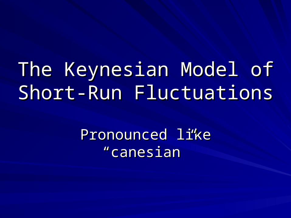
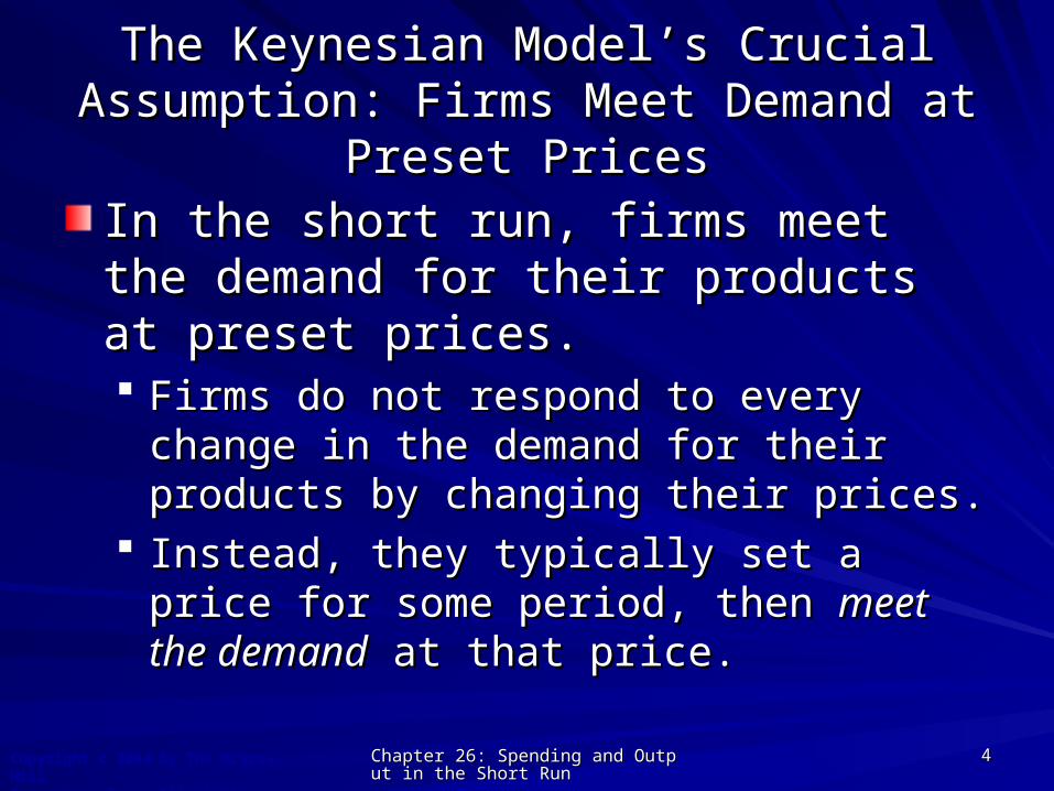
In the short run, firms meet the demand for In the short run, firms meet the demand for their products at preset prices.their products at preset prices. Firms do not respond to every change in the Firms do not respond to every change in the
demand for their products by changing their demand for their products by changing their prices.prices.
Instead, they typically set a price for some Instead, they typically set a price for some period, then period, then meet the demandmeet the demand at that price. at that price.
The Keynesian Model’s Crucial Assumption: The Keynesian Model’s Crucial Assumption: Firms Meet Demand at Preset PricesFirms Meet Demand at Preset Prices

Chapter 26: Spending and Output in theChapter 26: Spending and Output in the Short Run Short Run
55Copyright c 2004 by The McGraw-HillCompanies, Inc. All rights reserved.
In the short run, firms meet the demand for In the short run, firms meet the demand for their products at preset prices.their products at preset prices. By “meeting the demand,” we mean that firms By “meeting the demand,” we mean that firms
produce just enough to satisfy their customers produce just enough to satisfy their customers at the prices that have been set.at the prices that have been set.
The Keynesian Model’s Crucial Assumption: The Keynesian Model’s Crucial Assumption: Firms Meet Demand at Preset PricesFirms Meet Demand at Preset Prices
Chapter 26: Spending and Output in theChapter 26: Spending and Output in the Short Run Short Run
66Copyright c 2004 by The McGraw-HillCompanies, Inc. All rights reserved.
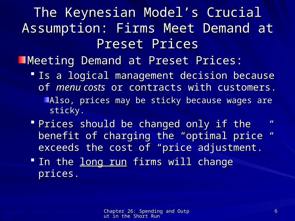
Meeting Demand at Preset Prices:Meeting Demand at Preset Prices: Is a logical management decision because of Is a logical management decision because of
menu costsmenu costs or contracts with customers. or contracts with customers.Also, prices may be sticky because wages are Also, prices may be sticky because wages are sticky.sticky.
Prices should be changed only if the benefit of Prices should be changed only if the benefit of charging the “optimal price” exceeds the cost charging the “optimal price” exceeds the cost of “price adjustment.”of “price adjustment.”
In the In the long runlong run firms will change prices. firms will change prices.
The Keynesian Model’s Crucial Assumption: The Keynesian Model’s Crucial Assumption: Firms Meet Demand at Preset PricesFirms Meet Demand at Preset Prices

Chapter 26: Spending and Output in theChapter 26: Spending and Output in the Short Run Short Run
77Copyright c 2004 by The McGraw-HillCompanies, Inc. All rights reserved.
Economic NaturalistEconomic Naturalist Will new technologies eliminate menu costs?Will new technologies eliminate menu costs?
Keynesian theory assumes that menu cost prevent Keynesian theory assumes that menu cost prevent firms from changing prices.firms from changing prices.
Many new technologies (bar codes) have reduced Many new technologies (bar codes) have reduced menu cost and increased price flexibility.menu cost and increased price flexibility.
The Keynesian Model’s Crucial Assumption: The Keynesian Model’s Crucial Assumption: Firms Meet Demand at Preset PricesFirms Meet Demand at Preset Prices

Chapter 26: Spending and Output in theChapter 26: Spending and Output in the Short Run Short Run
88Copyright c 2004 by The McGraw-HillCompanies, Inc. All rights reserved.
Economic NaturalistEconomic Naturalist Will new technologies eliminate menu costs?Will new technologies eliminate menu costs?
Pricing decisions also require market analysis, Pricing decisions also require market analysis, strategic considerations, and cost analysisstrategic considerations, and cost analysis
These factors are a component of menu costs, These factors are a component of menu costs, which technology may reduce but not eliminate.which technology may reduce but not eliminate.
The Keynesian Model’s Crucial Assumption: The Keynesian Model’s Crucial Assumption: Firms Meet Demand at Preset PricesFirms Meet Demand at Preset Prices
Chapter 26: Spending and Output in theChapter 26: Spending and Output in the Short Run Short Run
99Copyright c 2004 by The McGraw-HillCompanies, Inc. All rights reserved.
Wage Stickiness may lead to Wage Stickiness may lead to Price StickinessPrice Stickiness
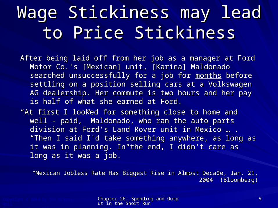
After being laid off from her job as a manager at Ford Motor After being laid off from her job as a manager at Ford Motor Co.'s [Mexican] unit, [Karina] Maldonado searched Co.'s [Mexican] unit, [Karina] Maldonado searched unsuccessfully for a job for unsuccessfully for a job for monthsmonths before settling on a before settling on a position selling cars at a Volkswagen AG dealership. Her position selling cars at a Volkswagen AG dealership. Her commute is two hours and her pay is half of what she commute is two hours and her pay is half of what she earned at Ford. earned at Ford.
““At first I looked for something close to home and well - At first I looked for something close to home and well - paid,” Maldonado, who ran the auto parts division at paid,” Maldonado, who ran the auto parts division at Ford's Land Rover unit in Mexico … . “Then I said I'd take Ford's Land Rover unit in Mexico … . “Then I said I'd take something anywhere, as long as it was in planning. In the something anywhere, as long as it was in planning. In the end, I didn't care as long as it was a job.” end, I didn't care as long as it was a job.”
““Mexican Jobless Rate Has Biggest Rise in Almost Decade, Jan. 21, 2004” Mexican Jobless Rate Has Biggest Rise in Almost Decade, Jan. 21, 2004” (Bloomberg)(Bloomberg)

Chapter 26: Spending and Output in theChapter 26: Spending and Output in the Short Run Short Run
1010Copyright c 2004 by The McGraw-HillCompanies, Inc. All rights reserved.
Aggregate ExpenditureAggregate Expenditure
Aggregate ExpenditureAggregate Expenditure Total spending on final goods and servicesTotal spending on final goods and services
NX G I C AE
AE = Planned AE + Unplanned AE

Chapter 26: Spending and Output in theChapter 26: Spending and Output in the Short Run Short Run
1111Copyright c 2004 by The McGraw-HillCompanies, Inc. All rights reserved.
Aggregate ExpenditureAggregate Expenditure
The Components of Aggregate The Components of Aggregate ExpenditureExpenditure
1.1. Consumer expenditure or Consumption (Consumer expenditure or Consumption (CC))Household spending on durables, nondurables, Household spending on durables, nondurables, and servicesand services
2.2. Investment (Investment (II))New capital goods spendingNew capital goods spending
New residential spendingNew residential spending
Increases in inventories (planned or unplanned)Increases in inventories (planned or unplanned)
Chapter 26: Spending and Output in theChapter 26: Spending and Output in the Short Run Short Run
1212Copyright c 2004 by The McGraw-HillCompanies, Inc. All rights reserved.
Aggregate ExpenditureAggregate Expenditure
The Components of Aggregate The Components of Aggregate ExpenditureExpenditure
3.3. Government purchasesGovernment purchasesFederal, state, and local spending on goods and Federal, state, and local spending on goods and servicesservices
4.4. Net exportsNet exportsExports - importsExports - imports
Chapter 26: Spending and Output in theChapter 26: Spending and Output in the Short Run Short Run
1313Copyright c 2004 by The McGraw-HillCompanies, Inc. All rights reserved.
Aggregate ExpenditureAggregate Expenditure
Planned Spending Versus Actual Planned Spending Versus Actual SpendingSpendingActual expenditures may not equal Actual expenditures may not equal PAE.PAE. Suppose a firm planned to sell 500,000 (and Suppose a firm planned to sell 500,000 (and
keep some as inventory) but only sold keep some as inventory) but only sold 450,000450,000
Then inventories are Then inventories are largerlarger than expected: than expected: I > I > planned Investment (planned Investment (IIPP))

Chapter 26: Spending and Output in theChapter 26: Spending and Output in the Short Run Short Run
1414Copyright c 2004 by The McGraw-HillCompanies, Inc. All rights reserved.
Planned Aggregate Planned Aggregate ExpenditureExpenditure
Planned Spending Versus Actual Planned Spending Versus Actual SpendingSpendingActual expenditures may not equal Actual expenditures may not equal PAE.PAE. Suppose a firm planned to sell 500,000 (and Suppose a firm planned to sell 500,000 (and
keep some as inventory) but sold 550,000keep some as inventory) but sold 550,000 If inventories are If inventories are smallersmaller than expected: than expected: I < II < IPP
Chapter 26: Spending and Output in theChapter 26: Spending and Output in the Short Run Short Run
1515Copyright c 2004 by The McGraw-HillCompanies, Inc. All rights reserved.
Planned Aggregate Planned Aggregate ExpenditureExpenditure
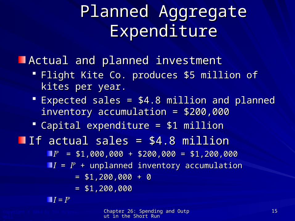
Actual and planned investmentActual and planned investment Flight Kite Co. produces $5 million of kites per year.Flight Kite Co. produces $5 million of kites per year. Expected sales = $4.8 million and planned inventory Expected sales = $4.8 million and planned inventory
accumulation = $200,000accumulation = $200,000 Capital expenditure = $1 millionCapital expenditure = $1 million
If actual sales = $4.8 millionIf actual sales = $4.8 millionIIPP = $1,000,000 + $200,000 = $1,200,000 = $1,000,000 + $200,000 = $1,200,000
II = = IIPP + unplanned inventory accumulation + unplanned inventory accumulation
= $1,200,000 + 0= $1,200,000 + 0
= $1,200,000= $1,200,000
I = II = IPP
Chapter 26: Spending and Output in theChapter 26: Spending and Output in the Short Run Short Run
1616Copyright c 2004 by The McGraw-HillCompanies, Inc. All rights reserved.
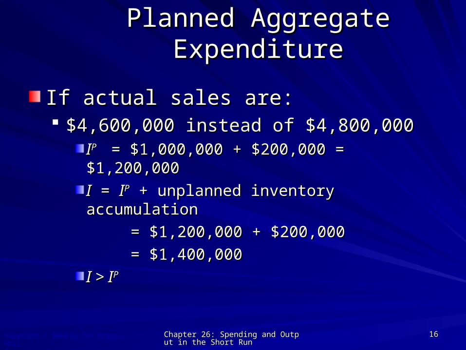
Planned Aggregate Planned Aggregate ExpenditureExpenditure
If actual sales are:If actual sales are: $4,600,000 instead of $4,800,000$4,600,000 instead of $4,800,000
IIPP = $1,000,000 + $200,000 = $1,200,000 = $1,000,000 + $200,000 = $1,200,000
II = = IIPP + unplanned inventory accumulation + unplanned inventory accumulation
= $1,200,000 + $200,000 = $1,200,000 + $200,000
= $1,400,000= $1,400,000
I > II > IPP

Chapter 26: Spending and Output in theChapter 26: Spending and Output in the Short Run Short Run
1717Copyright c 2004 by The McGraw-HillCompanies, Inc. All rights reserved.
Planned Aggregate Planned Aggregate ExpenditureExpenditure
If actual sales are:If actual sales are: $5,000,000 $5,000,000
IIPP = $1,000,000 + $200,000 = $1,200,000 = $1,000,000 + $200,000 = $1,200,000
II = = IIPP + unplanned inventory accumulation + unplanned inventory accumulation
= $1,200,000 = $1,200,000 –– $200,000 $200,000
= $1,000,000= $1,000,000 I < II < IPP

Chapter 26: Spending and Output in theChapter 26: Spending and Output in the Short Run Short Run
1818Copyright c 2004 by The McGraw-HillCompanies, Inc. All rights reserved.
Planned Aggregate Planned Aggregate ExpenditureExpenditure
Planned Aggregate ExpenditurePlanned Aggregate Expenditure
NX G I C PAE P
P

Chapter 26: Spending and Output in theChapter 26: Spending and Output in the Short Run Short Run
1919Copyright c 2004 by The McGraw-HillCompanies, Inc. All rights reserved.
Planned Aggregate Planned Aggregate ExpenditureExpenditure
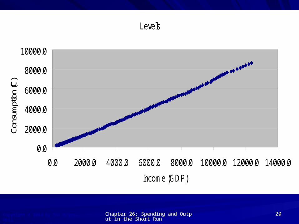
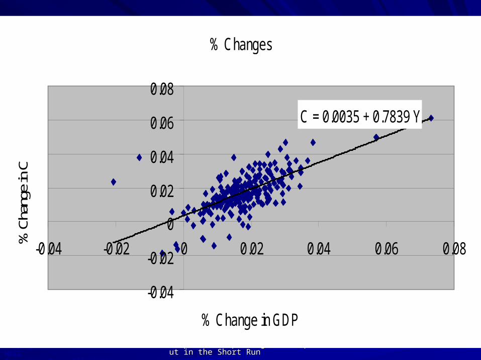
Consumer Spending and the EconomyConsumer Spending and the Economy Consumption (Consumption (CC) accounts for two thirds of ) accounts for two thirds of
total spending.total spending.
What determines Consumption?What determines Consumption?
Check out “Explaining Consumption.xls”Check out “Explaining Consumption.xls”
Chapter 26: Spending and Output in theChapter 26: Spending and Output in the Short Run Short Run
2020Copyright c 2004 by The McGraw-HillCompanies, Inc. All rights reserved.
U.S. Consumption and U.S. Consumption and Output, 1960-2001Output, 1960-2001
Levels
0.0
2000.0
4000.0
6000.0
8000.0
10000.0
0.0 2000.0 4000.0 6000.0 8000.0 10000.0 12000.0 14000.0
Income (GDP)
Con
sum
ptio
n (C
)
Chapter 26: Spending and Output in theChapter 26: Spending and Output in the Short Run Short Run
2121Copyright c 2004 by The McGraw-HillCompanies, Inc. All rights reserved.
% Changes
C = 0.0035 + 0.7839 Y
-0.04
-0.02
0
0.02
0.04
0.06
0.08
-0.04 -0.02 0 0.02 0.04 0.06 0.08
% Change in GDP
% C
hang
e in
C

Chapter 26: Spending and Output in theChapter 26: Spending and Output in the Short Run Short Run
2222Copyright c 2004 by The McGraw-HillCompanies, Inc. All rights reserved.
Planned Aggregate Planned Aggregate ExpenditureExpenditure
Consumer Spending and the EconomyConsumer Spending and the Economy The primary determinant of The primary determinant of C C is is disposable disposable
incomeincome or or Y – TY – T
Consumption FunctionConsumption Function The relationship between consumption The relationship between consumption
spending and its determinants, in particular, spending and its determinants, in particular, disposable (after-tax) incomedisposable (after-tax) income

Chapter 26: Spending and Output in theChapter 26: Spending and Output in the Short Run Short Run
2323Copyright c 2004 by The McGraw-HillCompanies, Inc. All rights reserved.
Planned Aggregate Planned Aggregate ExpenditureExpenditure
Relating Consumption to Income and Other Relating Consumption to Income and Other DeterminantsDeterminants The consumption function:The consumption function:
T)- c(Y C C
Consumption is a function of other factors (C) and disposable income (Y-T)

Chapter 26: Spending and Output in theChapter 26: Spending and Output in the Short Run Short Run
2424Copyright c 2004 by The McGraw-HillCompanies, Inc. All rights reserved.
Planned Aggregate Planned Aggregate ExpenditureExpenditure
C = a constant; represents the C = a constant; represents the non-incomenon-income determinants of determinants of CC. It is called . It is called autonomous autonomous consumptionconsumption Consumer optimismConsumer optimism WealthWealth Real interest ratesReal interest rates PricesPrices
T)- c(Y C C
Chapter 26: Spending and Output in theChapter 26: Spending and Output in the Short Run Short Run
2525Copyright c 2004 by The McGraw-HillCompanies, Inc. All rights reserved.
Planned Aggregate Planned Aggregate ExpenditureExpenditure
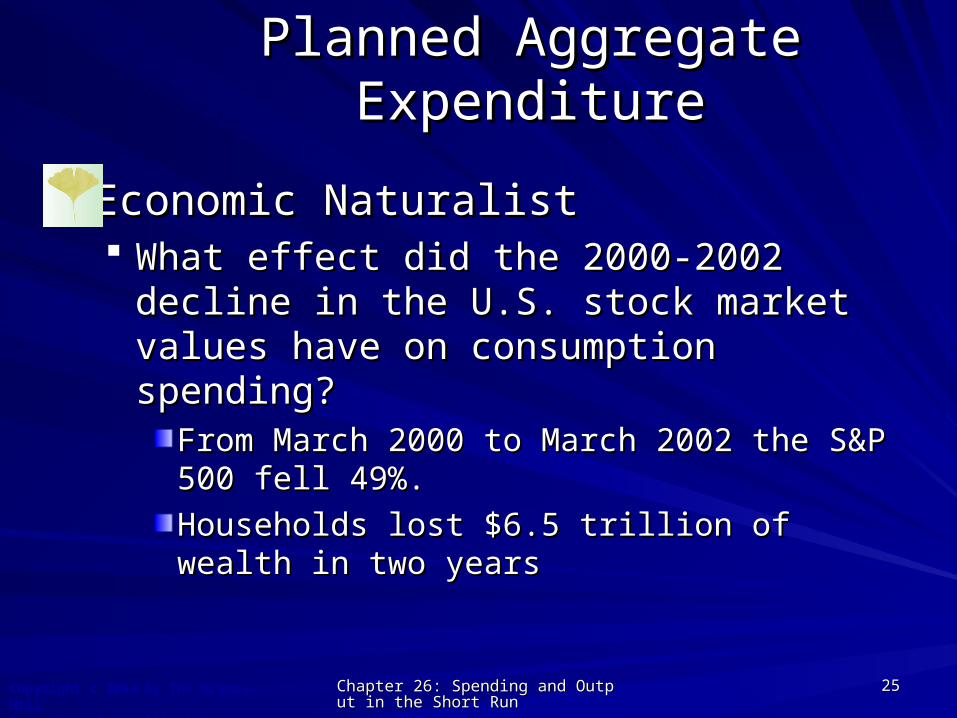
Economic NaturalistEconomic Naturalist What effect did the 2000-2002 decline in the What effect did the 2000-2002 decline in the
U.S. stock market values have on U.S. stock market values have on consumption spending?consumption spending?
From March 2000 to March 2002 the S&P 500 fell From March 2000 to March 2002 the S&P 500 fell 49%.49%.
Households lost $6.5 trillion of wealth in two yearsHouseholds lost $6.5 trillion of wealth in two years

Chapter 26: Spending and Output in theChapter 26: Spending and Output in the Short Run Short Run
2626Copyright c 2004 by The McGraw-HillCompanies, Inc. All rights reserved.
Planned Aggregate Planned Aggregate ExpenditureExpenditure
Economic NaturalistEconomic Naturalist $1 decrease in wealth reduces $1 decrease in wealth reduces CC
(autonomous consumption) by 3 to 7 (autonomous consumption) by 3 to 7 cents/yearcents/year
The $6.5 trillion loss could reduce The $6.5 trillion loss could reduce CC between between $195 and $455 billion$195 and $455 billion
Chapter 26: Spending and Output in theChapter 26: Spending and Output in the Short Run Short Run
2727Copyright c 2004 by The McGraw-HillCompanies, Inc. All rights reserved.
Planned Aggregate Planned Aggregate ExpenditureExpenditure
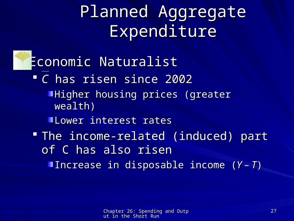
Economic NaturalistEconomic Naturalist CC has risen since 2002 has risen since 2002
Higher housing prices (greater wealth)Higher housing prices (greater wealth)
Lower interest ratesLower interest rates
The income-related (induced) part of C has The income-related (induced) part of C has also risenalso risen
Increase in disposable income (Increase in disposable income (Y – TY – T))
Chapter 26: Spending and Output in theChapter 26: Spending and Output in the Short Run Short Run
2828Copyright c 2004 by The McGraw-HillCompanies, Inc. All rights reserved.
Planned Aggregate Planned Aggregate ExpenditureExpenditure
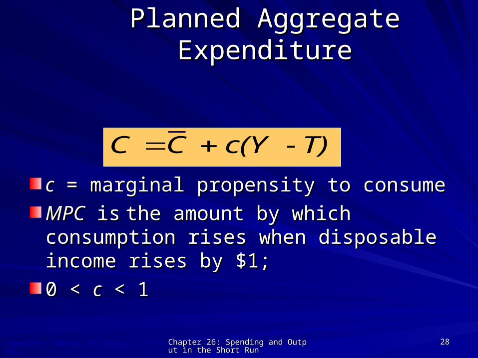
cc = marginal propensity to consume = marginal propensity to consume
MPCMPC is is the amount by which consumption the amount by which consumption rises when disposable income rises by $1;rises when disposable income rises by $1;
0 < 0 < cc < 1 < 1
T)- c(Y C C

Chapter 26: Spending and Output in theChapter 26: Spending and Output in the Short Run Short Run
2929Copyright c 2004 by The McGraw-HillCompanies, Inc. All rights reserved.
A Consumption FunctionA Consumption Function
Disposable income Y-T
Co
nsu
mp
tio
n s
pen
din
g C
Consumption function
Slope = c = MPCC
T)- c(Y C C

Chapter 26: Spending and Output in theChapter 26: Spending and Output in the Short Run Short Run
3030Copyright c 2004 by The McGraw-HillCompanies, Inc. All rights reserved.
What do we know so far?What do we know so far?
Planned Aggregate ExpenditurePlanned Aggregate Expenditure= C + I= C + IPP + G + NX + G + NX
Actual expenditures may not equal Actual expenditures may not equal PAEPAE If so, unplanned inventory (de)accumulation If so, unplanned inventory (de)accumulation
will occur.will occur.
Consumption depends positively on Consumption depends positively on disposable incomedisposable income (Income after taxes)(Income after taxes)

Chapter 26: Spending and Output in theChapter 26: Spending and Output in the Short Run Short Run
3131Copyright c 2004 by The McGraw-HillCompanies, Inc. All rights reserved.
Planned Aggregate Planned Aggregate ExpenditureExpenditure
Planned Aggregate Expenditure and Planned Aggregate Expenditure and OutputOutput The relationship between changes in The relationship between changes in
production and income and production and income and PAEPAEA large part of PAE is A large part of PAE is CC
CC depends on depends on YY
PAEPAE depends on depends on YYY
PAE
C
We still haven’t shown this connection

Chapter 26: Spending and Output in theChapter 26: Spending and Output in the Short Run Short Run
3232Copyright c 2004 by The McGraw-HillCompanies, Inc. All rights reserved.
Planned Aggregate Planned Aggregate ExpenditureExpenditure
ExampleExamplePAE = C + IPAE = C + IPP + G + NX + G + NX
C = C + c(Y – T)C = C + c(Y – T)
PAE = C + c(Y – T) + IPAE = C + c(Y – T) + IPP + G + NX + G + NX
C = C = 620; c = 0.8; 620; c = 0.8; T = T = 250;250;
IIPP = 220; = 220; GG = 300; = 300; NX = NX = 2020
From C to PAE, From C to PAE, algebraicallyalgebraically
For the moment we assume that only C depends on Y. Assume all other components of AE are exogenous.
Y
PAE
C

Chapter 26: Spending and Output in theChapter 26: Spending and Output in the Short Run Short Run
3333Copyright c 2004 by The McGraw-HillCompanies, Inc. All rights reserved.
Planned Aggregate Planned Aggregate ExpenditureExpenditure
Then:Then:
20 300 220 250) - 0.8( 620 Y PAE
20 300 220 0.8(250) - 0.8 620 Y PAE
20 300 220 2000.8 620 - Y PAE
Y- PAE 0.8200(620 20) 300 220
Y PAE 0.8 960
From C to PAE, numericallyFrom C to PAE, numerically

Chapter 26: Spending and Output in theChapter 26: Spending and Output in the Short Run Short Run
3434Copyright c 2004 by The McGraw-HillCompanies, Inc. All rights reserved.
Planned Aggregate Planned Aggregate ExpenditureExpenditure
Output, Y
Pla
nn
ed E
xpen
dit
ure
s
Consumption function
Slope = c = MPCC
T)- c(Y C C
From C to PAE, graphicallyFrom C to PAE, graphicallyPAE
Slope = c = MPCC+IP+G+NX
NXGICPAE P

Chapter 26: Spending and Output in theChapter 26: Spending and Output in the Short Run Short Run
3535Copyright c 2004 by The McGraw-HillCompanies, Inc. All rights reserved.
Planned Aggregate Planned Aggregate ExpenditureExpenditure
If Y increases by $1, If Y increases by $1, CC will increase by 80 will increase by 80 cents (cents (cc = 0.80) = 0.80)
And because And because CC is part of is part of PAE, …PAE, … PAEPAE increases by 80 cents ($1 X 0.80) increases by 80 cents ($1 X 0.80)
NX G I C Y PAE 0.8 960

Chapter 26: Spending and Output in theChapter 26: Spending and Output in the Short Run Short Run
3636Copyright c 2004 by The McGraw-HillCompanies, Inc. All rights reserved.
Planned Aggregate Planned Aggregate ExpenditureExpenditure
There are two parts to There are two parts to PAE:PAE: Autonomous expenditure (960)Autonomous expenditure (960)
Is independent of output: Does not vary Is independent of output: Does not vary when output changeswhen output changesIt varies with prices, consumer confidence, It varies with prices, consumer confidence, interest rates, wealth, etc.interest rates, wealth, etc.
Induced expenditure (0.8Induced expenditure (0.8YY))Depends on output (Depends on output (YY))
Y PAE 0.8 960

Chapter 26: Spending and Output in theChapter 26: Spending and Output in the Short Run Short Run
3737Copyright c 2004 by The McGraw-HillCompanies, Inc. All rights reserved.
Graphing the Expenditures Graphing the Expenditures FunctionFunction
(b)Real output
PAE
310
190
200 400 600
Slope = 0.6
McGraw-Hill/Irwin
(a)
200 400 600Real output
380
140
PAE
Slope = 0.6
(c)Real output
PAE
200 400 600
400
200
Slope = 0.5
Autonomous expenditure
ex
pe
nd
itu
re
ex
pe
nd
itu
re
ex
pe
nd
itu
re
Induced expenditure

Chapter 26: Spending and Output in theChapter 26: Spending and Output in the Short Run Short Run
3838Copyright c 2004 by The McGraw-HillCompanies, Inc. All rights reserved.
Planned Aggregate Planned Aggregate ExpenditureExpenditure
Autonomous expenditureAutonomous expenditure Is the part of expenditure that Is the part of expenditure that does notdoes not
depend on outputdepend on outputInduced expenditureInduced expenditure Is the part of expenditure that depends Is the part of expenditure that depends
on output (on output (YY))
Y PAE 0.8 960

Chapter 26: Spending and Output in theChapter 26: Spending and Output in the Short Run Short Run
3939Copyright c 2004 by The McGraw-HillCompanies, Inc. All rights reserved.
Short-run Equilibrium OutputShort-run Equilibrium Output
The Key Keynesian Assumption:The Key Keynesian Assumption:
Producers meet demand at preset prices Producers meet demand at preset prices in the short-run.in the short-run. Suppose planned demand for goods is higher Suppose planned demand for goods is higher
than production:than production: Instead of raising prices, firms will increase Instead of raising prices, firms will increase
production, until Y = PAE.production, until Y = PAE.

Chapter 26: Spending and Output in theChapter 26: Spending and Output in the Short Run Short Run
4040Copyright c 2004 by The McGraw-HillCompanies, Inc. All rights reserved.
Short-run Equilibrium OutputShort-run Equilibrium Output
Therefore,Therefore,
Y = PAEY = PAE
is a condition for economic equilibriumis a condition for economic equilibrium
(in the short run)(in the short run)
Chapter 26: Spending and Output in theChapter 26: Spending and Output in the Short Run Short Run
4141Copyright c 2004 by The McGraw-HillCompanies, Inc. All rights reserved.
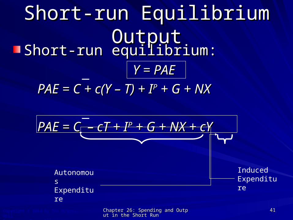
Short-run equilibrium:Short-run equilibrium:Y = PAEY = PAE
PAE = C + c(Y – T) + IPAE = C + c(Y – T) + IPP + G + NX + G + NX
PAE = C – cT + IPAE = C – cT + IPP + G + NX + cY + G + NX + cY
Induced Expenditure
Autonomous Expenditure
Short-run Equilibrium OutputShort-run Equilibrium Output

Chapter 26: Spending and Output in theChapter 26: Spending and Output in the Short Run Short Run
4242Copyright c 2004 by The McGraw-HillCompanies, Inc. All rights reserved.
Short-run Equilibrium OutputShort-run Equilibrium Output The level of output at which output The level of output at which output Y Y equals equals
planned aggregate expenditure planned aggregate expenditure PAEPAE Short-runShort-run equilibrium output: the level of equilibrium output: the level of
output that prevails as long as prices are output that prevails as long as prices are predetermined.predetermined.
Y = PAEY = PAE
Short-run Equilibrium OutputShort-run Equilibrium Output
Chapter 26: Spending and Output in theChapter 26: Spending and Output in the Short Run Short Run
4343Copyright c 2004 by The McGraw-HillCompanies, Inc. All rights reserved.
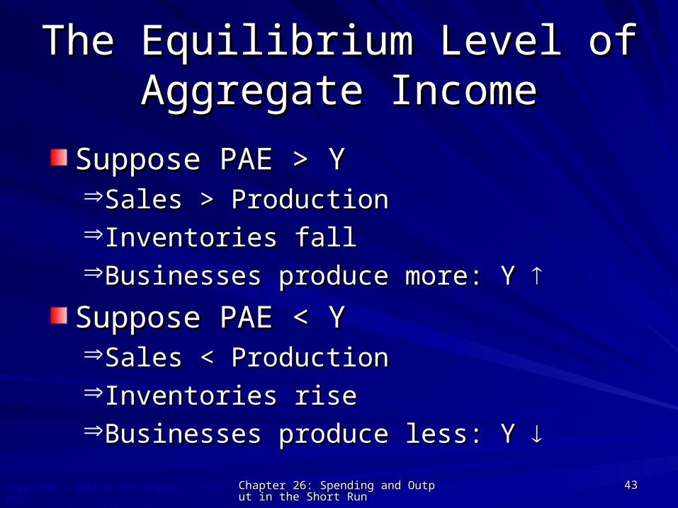
The Equilibrium Level of The Equilibrium Level of Aggregate IncomeAggregate Income
Suppose PAE > YSuppose PAE > YSales > ProductionSales > ProductionInventories fallInventories fallBusinesses produce more: Y Businesses produce more: Y
Suppose PAE < YSuppose PAE < YSales < ProductionSales < ProductionInventories riseInventories riseBusinesses produce less: Y Businesses produce less: Y

Chapter 26: Spending and Output in theChapter 26: Spending and Output in the Short Run Short Run
4444Copyright c 2004 by The McGraw-HillCompanies, Inc. All rights reserved.
Planned Aggregate Planned Aggregate ExpenditureExpenditure
Short-run Equilibrium OutputShort-run Equilibrium Output1.1. Y = PAEY = PAE
2.2. PAE = C + c(Y – T) + IPAE = C + c(Y – T) + IPP + G + NX + G + NX
This is a system with two equations and two This is a system with two equations and two unknowns.unknowns.
Solve it by putting equation 2 into equation 1:Solve it by putting equation 2 into equation 1:
Y = C + c(Y – T) + IY = C + c(Y – T) + IPP + G + NX + G + NX

Chapter 26: Spending and Output in theChapter 26: Spending and Output in the Short Run Short Run
4545Copyright c 2004 by The McGraw-HillCompanies, Inc. All rights reserved.
Numerical Determination of Numerical Determination of Short-Run Equilibrium OutputShort-Run Equilibrium Output
(1) Output
Y
4,000 4,160 -160 No
4,200
4,400
4,600
4,800
5,000
5,200
(2) Planned aggregate expenditure
PAE = 960 + 0.8Y
(3)
Y - PAE
(4)
Y = PAE?
•Equilibrium: Y = PAE; Y (4,800) = PAE (4,800)•If Y = 4,000 < PAE = 960 + .8(4000) = 4,160•If Y = 5,000 > PAE = 960 + .8(5,000) = 4,960
4,320 -120 No
4,480 -80 No
4,640 -40 No
4,800 0 Yes
4,960 40 No
5,120 80 No
Chapter 26: Spending and Output in theChapter 26: Spending and Output in the Short Run Short Run
4646Copyright c 2004 by The McGraw-HillCompanies, Inc. All rights reserved.
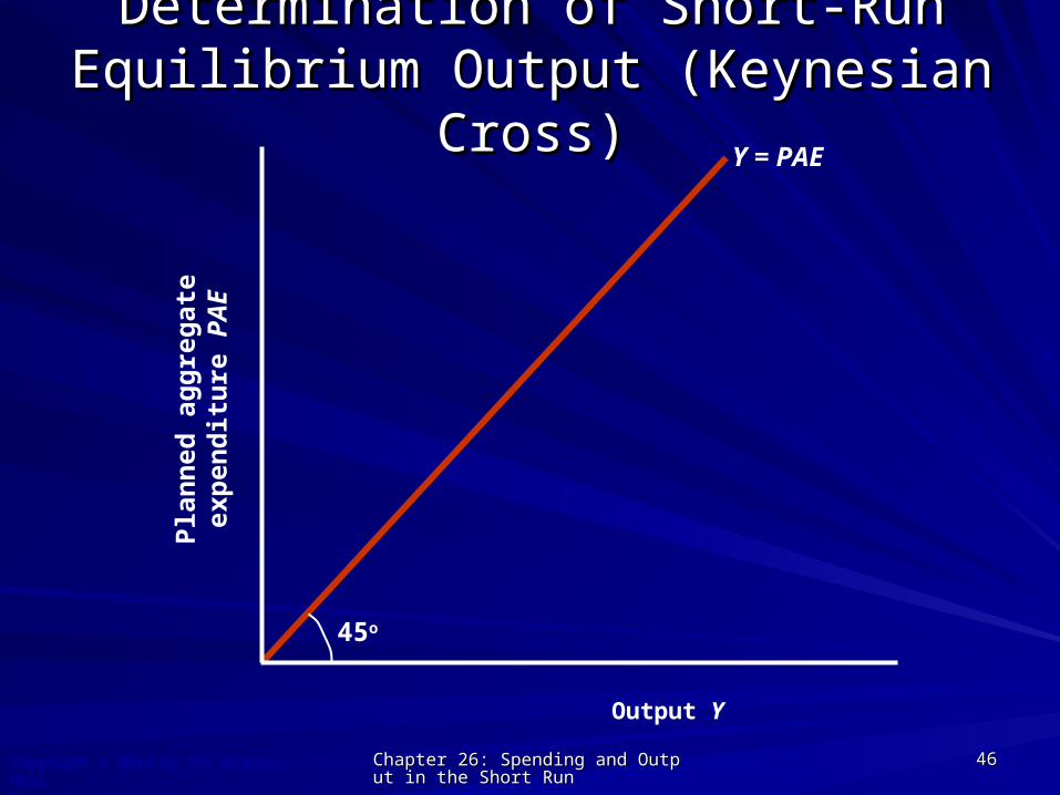
Determination of Short-Run Equilibrium Determination of Short-Run Equilibrium Output (Keynesian Cross)Output (Keynesian Cross)
Output Y
Pla
nn
ed a
gg
reg
ate
exp
end
itu
re
PA
E
45o
Y = PAE

Chapter 26: Spending and Output in theChapter 26: Spending and Output in the Short Run Short Run
4747Copyright c 2004 by The McGraw-HillCompanies, Inc. All rights reserved.
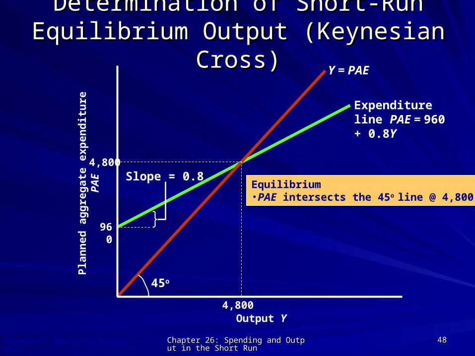
Determination of Short-Run Equilibrium Determination of Short-Run Equilibrium Output (Keynesian Cross)Output (Keynesian Cross)
Output Y
Pla
nn
ed a
gg
reg
ate
exp
end
itu
re P
AE
960
Expenditure line PAE = 960 + 0.8Y
Slope = 0.8
Chapter 26: Spending and Output in theChapter 26: Spending and Output in the Short Run Short Run
4848Copyright c 2004 by The McGraw-HillCompanies, Inc. All rights reserved.
Determination of Short-Run Equilibrium Determination of Short-Run Equilibrium Output (Keynesian Cross)Output (Keynesian Cross)
Output Y
Pla
nn
ed a
gg
reg
ate
exp
end
itu
re P
AE
960
Expenditure line PAE = 960 + 0.8Y
Slope = 0.8
45o
Y = PAE
4,800
Equilibrium• PAE intersects the 45o line @ 4,800
4,800

Chapter 26: Spending and Output in theChapter 26: Spending and Output in the Short Run Short Run
4949Copyright c 2004 by The McGraw-HillCompanies, Inc. All rights reserved.
The Equilibrium Level of The Equilibrium Level of Aggregate IncomeAggregate Income
Suppose PAE > YSuppose PAE > YSales > ProductionSales > ProductionInventories fallInventories fallBusinesses produce more: Y Businesses produce more: Y
Suppose PAE < YSuppose PAE < YSales < ProductionSales < ProductionInventories riseInventories riseBusinesses produce less: Y Businesses produce less: Y

Chapter 26: Spending and Output in theChapter 26: Spending and Output in the Short Run Short Run
5050Copyright c 2004 by The McGraw-HillCompanies, Inc. All rights reserved.
The Equilibrium Level of The Equilibrium Level of Aggregate IncomeAggregate Income
Remember Inventories are a kind of Remember Inventories are a kind of investment:investment: Planned changes in inventory are part of IPlanned changes in inventory are part of IPP.. Unplanned changes in inventory are part of I Unplanned changes in inventory are part of I
(but not of I(but not of IPP).).Unplanned inventory changes make sure Unplanned inventory changes make sure actual actual aggregate expenditures = income all the time.aggregate expenditures = income all the time.
When PAE=Y, unplanned inventory changes = 0.When PAE=Y, unplanned inventory changes = 0.

Chapter 26: Spending and Output in theChapter 26: Spending and Output in the Short Run Short Run
5151Copyright c 2004 by The McGraw-HillCompanies, Inc. All rights reserved.
Determination of Short-Run Equilibrium Determination of Short-Run Equilibrium Output (Keynesian Cross)Output (Keynesian Cross)
Output Y
Pla
nn
ed a
gg
reg
ate
exp
end
itu
re P
AE
960
Expenditure line PAE = 960 + 0.8Y
45o
Y = PAE
4,800
Disequilibrium• If PAE > 4,800,
PAE > Y Inventories fall• If PAE < 4,800,
PAE < Y Inventories rise
4,800
PAE<Y
PAE>Y

Chapter 26: Spending and Output in theChapter 26: Spending and Output in the Short Run Short Run
5252Copyright c 2004 by The McGraw-HillCompanies, Inc. All rights reserved.
A Decline In Planned A Decline In Planned Spending Leads To A RecessionSpending Leads To A Recession
Output Y
Pla
nn
ed a
gg
reg
ate
exp
end
itu
re P
AE
960
E
Expenditure line PAE = 960 + 0.8Y
45o
Y = PAE
4,800Y*
Suppose the economy starts from short-run equilibrium,
And suppose that Y = Y*, actual equilibrium output = potential output.(This isn’t always so).
Chapter 26: Spending and Output in theChapter 26: Spending and Output in the Short Run Short Run
5353Copyright c 2004 by The McGraw-HillCompanies, Inc. All rights reserved.
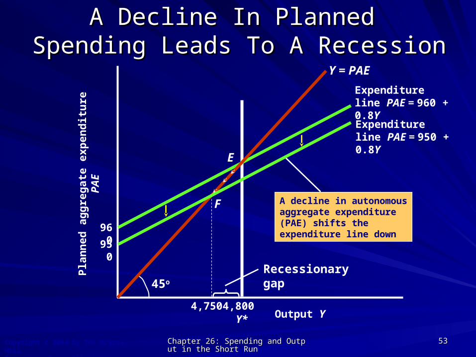
A Decline In Planned A Decline In Planned Spending Leads To A RecessionSpending Leads To A Recession
Output Y
Pla
nn
ed a
gg
reg
ate
exp
end
itu
re P
AE
960
E
Expenditure line PAE = 960 + 0.8Y
45o
Y = PAE
4,800Y*
Recessionary gap
A decline in autonomous aggregate expenditure (PAE) shifts the expenditure line down
F
4,750
Expenditure line PAE = 950 + 0.8Y
950

Chapter 26: Spending and Output in theChapter 26: Spending and Output in the Short Run Short Run
5454Copyright c 2004 by The McGraw-HillCompanies, Inc. All rights reserved.
Planned Aggregate Planned Aggregate ExpenditureExpenditure
Autonomous Spending can fall because…Autonomous Spending can fall because… The exchange rate appreciates.The exchange rate appreciates.
Makes exports more expensive, Makes exports more expensive, NX < 0.NX < 0. The government cuts the budget deficit.The government cuts the budget deficit.
G < 0 G < 0 T > 0, government expenditure falls or taxes T > 0, government expenditure falls or taxes rise.rise.
The Central Bank raises interest rates.The Central Bank raises interest rates.IIPP < 0, investment falls. < 0, investment falls.
Prices rise.Prices rise.The purchasing power of consumers’ wealth falls,The purchasing power of consumers’ wealth falls, C < 0, autonomous consumption falls.C < 0, autonomous consumption falls.

Chapter 26: Spending and Output in theChapter 26: Spending and Output in the Short Run Short Run
5555Copyright c 2004 by The McGraw-HillCompanies, Inc. All rights reserved.
(1) Output
Y
4,000 4,160 -160 No
4,200
4,400
4,600
4,800
5,000
5,200
(2) Planned aggregate expenditure
PAE = 960 + 0.8Y
(3)
Y - PAE
(4)
Y = PAE?
•Equilibrium: Y = PAE; Y (4,800) = PAE (4,800)•If Y = 4,000 < PAE = 960 + .8(4000) = 4,160•If Y = 5,000 > PAE = 960 + .8(5,000) = 4,960
4,320 -120 No
4,480 -80 No
4,640 -40 No
4,800 0 Yes
4,960 40 No
5,120 80 No
Original Aggregate ExpenditureOriginal Aggregate Expenditure

Chapter 26: Spending and Output in theChapter 26: Spending and Output in the Short Run Short Run
5656Copyright c 2004 by The McGraw-HillCompanies, Inc. All rights reserved.
(1) Output
Y
4,600 4,630 -30 No
4,650
4,700
4,750
4,800
4,850
4,900
4,950
5,000
(2) Planned aggregate expenditure
PAE = 950 + 0.8Y
(3)
Y - PAE
(4)
Y = PAE?
•If Y = 4,800 then PAE = 4,790 < Y•Y = PAE @ 4,750•Output Gap: Y* (4,800) > Y (4,750)
4,670 -20 No
4,710 -10 No
4,750 0 Yes
4,790 10 No
4,830 20 No
4,870 30 No
4,910 40 No
4,950 50 No
Short-Run Short-Run Equilibrium Output Equilibrium Output After A Fall In SpendingAfter A Fall In Spending

Chapter 26: Spending and Output in theChapter 26: Spending and Output in the Short Run Short Run
5757Copyright c 2004 by The McGraw-HillCompanies, Inc. All rights reserved.
Planned Aggregate Planned Aggregate ExpenditureExpenditure
Other factors remaining constant, a Other factors remaining constant, a declinedecline in autonomous spending causes in autonomous spending causes short-run equilibrium output to fall.short-run equilibrium output to fall. If the economy started at full employment, this If the economy started at full employment, this
creates a recessionary gap.creates a recessionary gap.
A decrease in autonomous spending can A decrease in autonomous spending can be caused by a reduction in be caused by a reduction in C, IC, IPP, G, , G, and/orand/or NX. NX.

Chapter 26: Spending and Output in theChapter 26: Spending and Output in the Short Run Short Run
5858Copyright c 2004 by The McGraw-HillCompanies, Inc. All rights reserved.
An Increase In Planned An Increase In Planned Spending Leads To An ExpansionSpending Leads To An Expansion
Output Y
Pla
nn
ed a
gg
reg
ate
exp
end
itu
re P
AE
960
E
Expenditure line PAE = 960 + 0.8Y
45o
Y = PAE
4,800Y*
Expansionary gap
Expenditure line PAE = 980 + 0.8Y
An increase in autonomous aggregate expenditure shifts the expenditure line up
F
4,900
980
Chapter 26: Spending and Output in theChapter 26: Spending and Output in the Short Run Short Run
5959Copyright c 2004 by The McGraw-HillCompanies, Inc. All rights reserved.
Planned Aggregate Planned Aggregate ExpenditureExpenditure
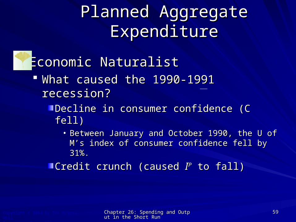
Economic NaturalistEconomic Naturalist What caused the 1990-1991 recession?What caused the 1990-1991 recession?
Decline in consumer confidence (C fell)Decline in consumer confidence (C fell)• Between January and October 1990, the U of M’s index Between January and October 1990, the U of M’s index
of consumer confidence fell by 31%.of consumer confidence fell by 31%.
Credit crunch (caused Credit crunch (caused IIPP to fall) to fall)

Chapter 26: Spending and Output in theChapter 26: Spending and Output in the Short Run Short Run
6060Copyright c 2004 by The McGraw-HillCompanies, Inc. All rights reserved.
0
20
40
60
80
100
120Ja
n-9
0
Fe
b-9
0
Ma
r-9
0
Ap
r-9
0
Ma
y-9
0
Jun
-90
Jul-
90
Au
g-9
0
Se
p-9
0
Oct
-90
No
v-9
0
De
c-9
0
Jan
-91
Fe
b-9
1
Ma
r-9
1
Ap
r-9
1
Ma
y-9
1
Jun
-91
Jul-
91
Au
g-9
1
Se
p-9
1
Oct
-91
No
v-9
1
De
c-9
1
Cons Confidence 90-91 Cons Confidence 2005
September 2005
February 2005
August1990
January 1990
Chapter 26: Spending and Output in theChapter 26: Spending and Output in the Short Run Short Run
6161Copyright c 2004 by The McGraw-HillCompanies, Inc. All rights reserved.
Planned Aggregate Planned Aggregate ExpenditureExpenditure
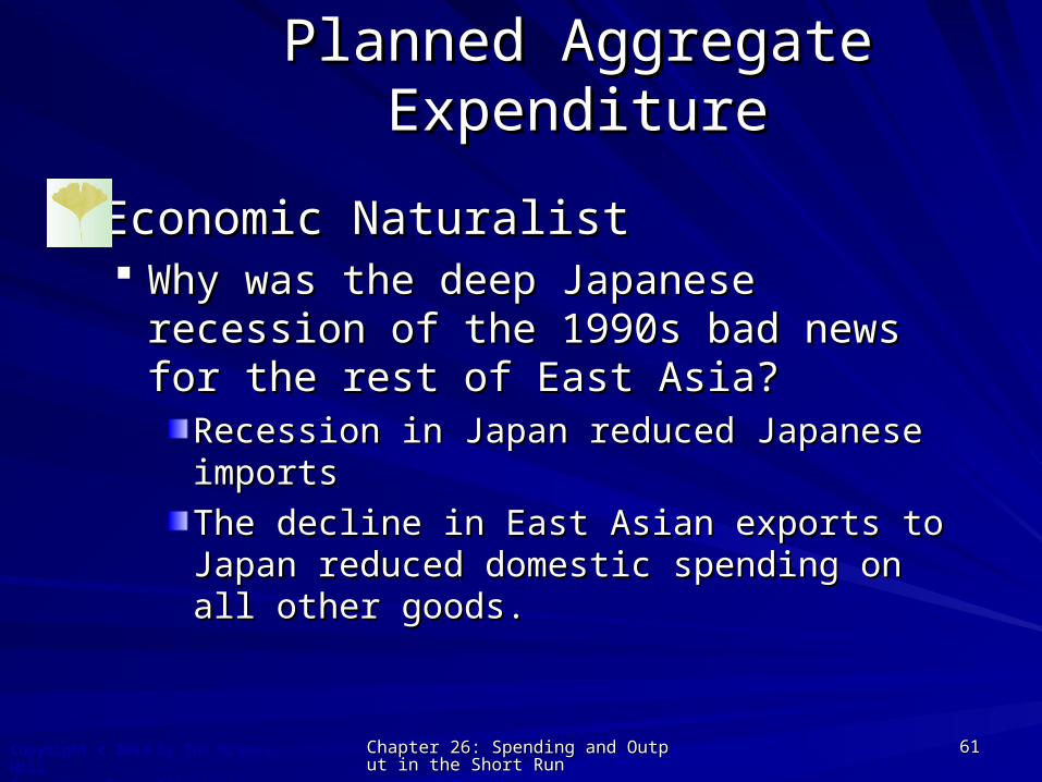
Economic NaturalistEconomic Naturalist Why was the deep Japanese recession of the Why was the deep Japanese recession of the
1990s bad news for the rest of East Asia?1990s bad news for the rest of East Asia?Recession in Japan reduced Japanese importsRecession in Japan reduced Japanese imports
The decline in East Asian exports to Japan The decline in East Asian exports to Japan reduced domestic spending on all other goods.reduced domestic spending on all other goods.
Chapter 26: Spending and Output in theChapter 26: Spending and Output in the Short Run Short Run
6262Copyright c 2004 by The McGraw-HillCompanies, Inc. All rights reserved.
Planned Aggregate Planned Aggregate ExpenditureExpenditure
Economic NaturalistEconomic Naturalist What caused the 2001 recession in the United What caused the 2001 recession in the United
States?States?Reduction in investment spendingReduction in investment spending

Chapter 26: Spending and Output in theChapter 26: Spending and Output in the Short Run Short Run
6363Copyright c 2004 by The McGraw-HillCompanies, Inc. All rights reserved.
Investment / GDP
13%
14%
15%
16%
17%
18%

Chapter 26: Spending and Output in theChapter 26: Spending and Output in the Short Run Short Run
6464Copyright c 2004 by The McGraw-HillCompanies, Inc. All rights reserved.
What do we know so far?What do we know so far?
Expenditure is of two kinds:Expenditure is of two kinds:autonomous and induced.autonomous and induced.
Producers meet demandProducers meet demandat preset prices in theat preset prices in theshort-run, so Y=PAEshort-run, so Y=PAEindicates equilibrium.indicates equilibrium.
If PAE > Y, production increases.If PAE > Y, production increases.
Changes in Changes in autonomousautonomous PAE change PAE change equilibrium Y.equilibrium Y.
Y
PA
E
PAE
45o
Y = PAE

The MultiplierThe Multiplier
Chapter 26: Spending and Output in theChapter 26: Spending and Output in the Short Run Short Run
6666Copyright c 2004 by The McGraw-HillCompanies, Inc. All rights reserved.
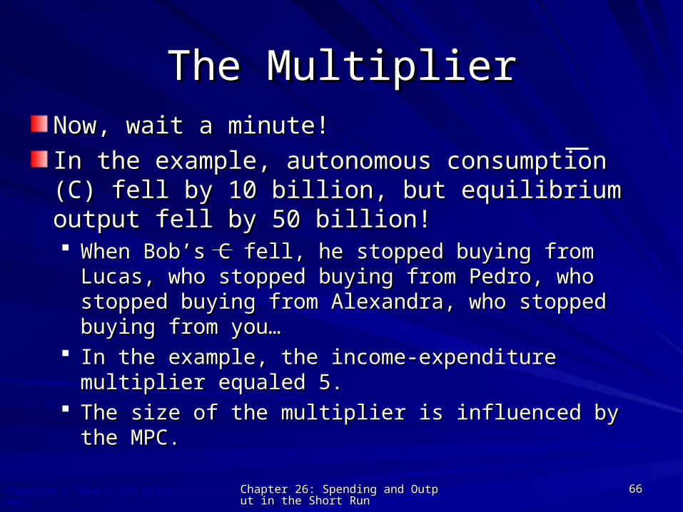
Now, wait a minute!Now, wait a minute!
In the example, autonomous consumption (C) fell In the example, autonomous consumption (C) fell by 10 billion, but equilibrium output fell by 50 by 10 billion, but equilibrium output fell by 50 billion!billion! When Bob’s C fell, he stopped buying from Lucas, who When Bob’s C fell, he stopped buying from Lucas, who
stopped buying from Pedro, who stopped buying from stopped buying from Pedro, who stopped buying from Alexandra, who stopped buying from you…Alexandra, who stopped buying from you…
In the example, the income-expenditure multiplier In the example, the income-expenditure multiplier equaled 5.equaled 5.
The size of the multiplier is influenced by the MPC.The size of the multiplier is influenced by the MPC.
The MultiplierThe Multiplier

Chapter 26: Spending and Output in theChapter 26: Spending and Output in the Short Run Short Run
6767Copyright c 2004 by The McGraw-HillCompanies, Inc. All rights reserved.
The First Five Steps of a The First Five Steps of a MultiplierMultiplier
Multiplier = 1/(1-0.4) = 1.7
100
40
16 6.4 2.56
MPC = 0.4
G increases by 100: they buy $100 worth of staples from Bob.
Bob’s income increases by 100. He spends 40% of it on Kate’s bikes,according to his MPC = 0.4.
Kate’s income rises by 40, so she spends 40% of it on Jason’s burgers.
Jason’s income rises by 16, so he spends 40% of it on Susan’s vinyl siding.
Susan’s income increases by 6.4, so she spends 40% of it on Peter’s travel agency services.
Peter’s income rises by 2.56, so …
Chapter 26: Spending and Output in theChapter 26: Spending and Output in the Short Run Short Run
6868Copyright c 2004 by The McGraw-HillCompanies, Inc. All rights reserved.
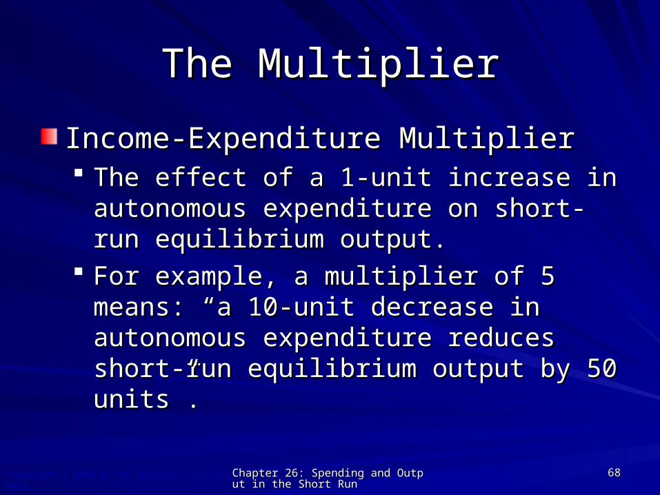
Income-Expenditure MultiplierIncome-Expenditure Multiplier The effect of a 1-unit increase in autonomous The effect of a 1-unit increase in autonomous
expenditure on short-run equilibrium output.expenditure on short-run equilibrium output. For example, a multiplier of 5 means: “a 10-For example, a multiplier of 5 means: “a 10-
unit decrease in autonomous expenditure unit decrease in autonomous expenditure reduces short-run equilibrium output by 50 reduces short-run equilibrium output by 50 units”.units”.
The MultiplierThe Multiplier
Chapter 26: Spending and Output in theChapter 26: Spending and Output in the Short Run Short Run
6969Copyright c 2004 by The McGraw-HillCompanies, Inc. All rights reserved.
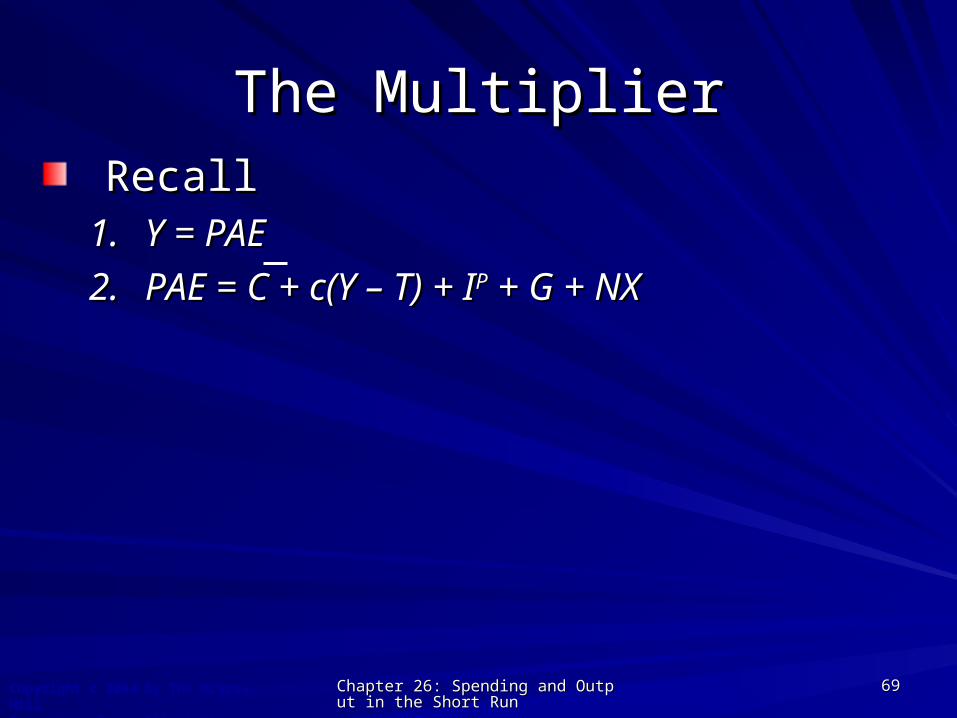
RecallRecall1.1. Y = PAEY = PAE
2.2. PAE = C + c(Y – T) + IPAE = C + c(Y – T) + IPP + G + NX + G + NX
The MultiplierThe Multiplier
Chapter 26: Spending and Output in theChapter 26: Spending and Output in the Short Run Short Run
7070Copyright c 2004 by The McGraw-HillCompanies, Inc. All rights reserved.
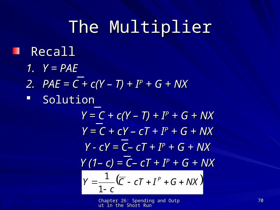
RecallRecall1.1. Y = PAEY = PAE
2.2. PAE = C + c(Y – T) + IPAE = C + c(Y – T) + IPP + G + NX + G + NX SolutionSolution
Y = C + c(Y – T) + IY = C + c(Y – T) + IPP + G + NX + G + NX
Y = C + cY – cT + IY = C + cY – cT + IPP + G + NX + G + NX
Y - cY = C– cT + IY - cY = C– cT + IPP + G + NX + G + NX
Y (1– c) = C– cT + IY (1– c) = C– cT + IPP + G + NX + G + NX
NXGIcTCc
Y P
1
1
The MultiplierThe Multiplier
Chapter 26: Spending and Output in theChapter 26: Spending and Output in the Short Run Short Run
7171Copyright c 2004 by The McGraw-HillCompanies, Inc. All rights reserved.
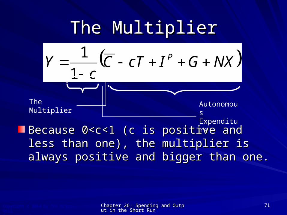
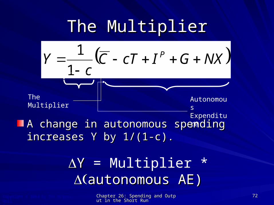
The MultiplierThe Multiplier
Because 0<c<1 (c is positive and less than one), Because 0<c<1 (c is positive and less than one), the multiplier is always positive and bigger than the multiplier is always positive and bigger than one.one.
NXGIcTCc
Y P
1
1
Autonomous Expenditure
The Multiplier
Chapter 26: Spending and Output in theChapter 26: Spending and Output in the Short Run Short Run
7272Copyright c 2004 by The McGraw-HillCompanies, Inc. All rights reserved.
The MultiplierThe Multiplier
A change in autonomous spending increases Y A change in autonomous spending increases Y by 1/(1-c).by 1/(1-c).
NXGIcTCc
Y P
1
1
Autonomous Expenditure
The Multiplier
YY = Multiplier * autonomous AE)autonomous AE)

Chapter 26: Spending and Output in theChapter 26: Spending and Output in the Short Run Short Run
7373Copyright c 2004 by The McGraw-HillCompanies, Inc. All rights reserved.
The MultiplierThe Multiplier
NXGIcTCc
Y P
1
1
Autonomous Expenditure
The Multiplier
Multiplier =YY
autonomous AE)autonomous AE)

Chapter 26: Spending and Output in theChapter 26: Spending and Output in the Short Run Short Run
7474Copyright c 2004 by The McGraw-HillCompanies, Inc. All rights reserved.
The MultiplierThe Multiplier
NXGIcTCc
Y P
1
1
Previously we assumedPreviously we assumedC = C = 620; c = 0.8; 620; c = 0.8; T = T = 250;250;
IIPP = 220; = 220; GG = 300; = 300; NX = NX = 2020
Plugging this in we getPlugging this in we get
Which takes a lot less work than Table 26.1Which takes a lot less work than Table 26.1
480020300220)250(8.06208.01
1
Y

Chapter 26: Spending and Output in theChapter 26: Spending and Output in the Short Run Short Run
7575Copyright c 2004 by The McGraw-HillCompanies, Inc. All rights reserved.
The MultiplierThe Multiplier
NXGIcTCc
Y P
1
1
Suppose nowSuppose nowC = C = 820; c = 0.7; 820; c = 0.7; T = T = 600;600;
IIPP = 600; = 600; GG = 600; = 600; NX = NX = 200200
Plugging this in we getPlugging this in we get
Which takes a lot less work than Exercise 26.1Which takes a lot less work than Exercise 26.1
6000200600600)600(7.08207.01
1
Y

Chapter 26: Spending and Output in theChapter 26: Spending and Output in the Short Run Short Run
7676Copyright c 2004 by The McGraw-HillCompanies, Inc. All rights reserved.
The Multiplier EquationThe Multiplier Equation
As the As the MPCMPC increases, the multiplier increases, the multiplier increases:increases:
MPC Multiplier = 1/(1-MPC)
MPC Multiplier = 1/(1-MPC)
0.3 1.4 0.75 4
0.4 1.7 0.8 5
0.5 2.0 0.9 10
Chapter 26: Spending and Output in theChapter 26: Spending and Output in the Short Run Short Run
7777Copyright c 2004 by The McGraw-HillCompanies, Inc. All rights reserved.
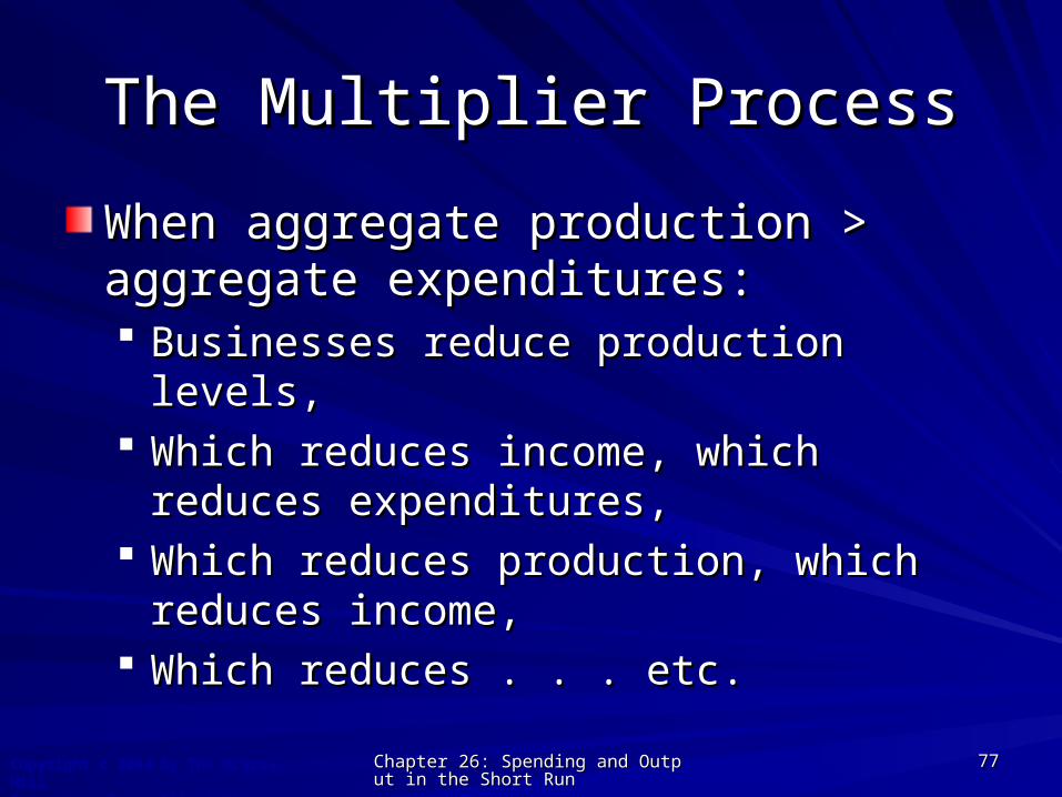
The Multiplier ProcessThe Multiplier Process
When aggregate production > aggregate When aggregate production > aggregate expenditures:expenditures: Businesses reduce production levels,Businesses reduce production levels, Which reduces income, which reduces Which reduces income, which reduces
expenditures,expenditures, Which reduces production, which reduces Which reduces production, which reduces
income,income, Which reduces . . . etc.Which reduces . . . etc.

Chapter 26: Spending and Output in theChapter 26: Spending and Output in the Short Run Short Run
7878Copyright c 2004 by The McGraw-HillCompanies, Inc. All rights reserved.
The Multiplier ProcessThe Multiplier Process
The process ends when aggregate The process ends when aggregate production equals aggregate expenditures.production equals aggregate expenditures.
Firms are selling all they produce, so they Firms are selling all they produce, so they have no reason to change their production have no reason to change their production levels.levels.

Chapter 26: Spending and Output in theChapter 26: Spending and Output in the Short Run Short Run
7979Copyright c 2004 by The McGraw-HillCompanies, Inc. All rights reserved.
The Multiplier ProcessThe Multiplier Process
$7,000
5,500
4,750
4,000
2,5002,000
Real income (in dollars)$1,000B
$4,000C
$7,000A
B1
B2
A2
A1
Y=PAE
PAE
Real
exp
endi
ture
s
Chapter 26: Spending and Output in theChapter 26: Spending and Output in the Short Run Short Run
8080Copyright c 2004 by The McGraw-HillCompanies, Inc. All rights reserved.
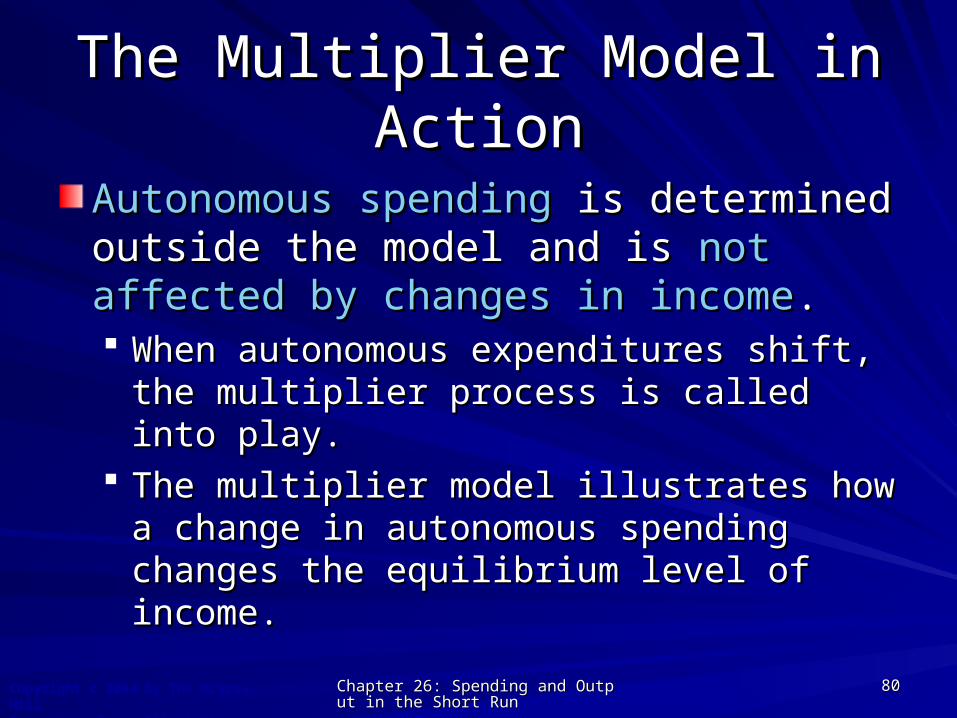
The Multiplier Model in ActionThe Multiplier Model in Action
Autonomous spendingAutonomous spending is determined is determined outside the model and is outside the model and is not affected by not affected by changes in incomechanges in income.. When autonomous expenditures shift, the When autonomous expenditures shift, the
multiplier process is called into play.multiplier process is called into play. The multiplier model illustrates how a change The multiplier model illustrates how a change
in autonomous spending changes the in autonomous spending changes the equilibrium level of income.equilibrium level of income.

Chapter 26: Spending and Output in theChapter 26: Spending and Output in the Short Run Short Run
8181Copyright c 2004 by The McGraw-HillCompanies, Inc. All rights reserved.
The Steps of the Multiplier The Steps of the Multiplier ProcessProcess
The The income adjustment process income adjustment process is directly is directly related to the multiplier.related to the multiplier.
Any initial shock (a change in autonomous Any initial shock (a change in autonomous PAEPAE) is multiplied in the multiplier process.) is multiplied in the multiplier process.
The multiplier process repeats itself again The multiplier process repeats itself again and again until a new equilibrium level is and again until a new equilibrium level is finally reached.finally reached.

Chapter 26: Spending and Output in theChapter 26: Spending and Output in the Short Run Short Run
8282Copyright c 2004 by The McGraw-HillCompanies, Inc. All rights reserved.
Shifts in the Planned Aggregate Shifts in the Planned Aggregate Expenditure CurveExpenditure Curve
200
PAE=5000+0.5Y
Y=PAE
200
25
50
100
PAE=4800+0.5Y
400
400
)200(0.5-1
1Y
NX)GIC(c-1
1Y P

Chapter 26: Spending and Output in theChapter 26: Spending and Output in the Short Run Short Run
8383Copyright c 2004 by The McGraw-HillCompanies, Inc. All rights reserved.
Shifts in the Planned Aggregate Shifts in the Planned Aggregate Expenditure CurveExpenditure Curve
400
)100(0.75-1
1Y
NX)GIC(c-1
1Y P
PAE=4900+0.75YY=PAE
42.19
100
PAE=4800+0.75Y
400
75
56.25

Chapter 26: Spending and Output in theChapter 26: Spending and Output in the Short Run Short Run
8484Copyright c 2004 by The McGraw-HillCompanies, Inc. All rights reserved.
Shifts in the PAE curveShifts in the PAE curve
Why does the PAE curve shift?Why does the PAE curve shift? Because C, IBecause C, IPP, G, T, or NX change exogenously., G, T, or NX change exogenously.
What happens if autonomous spending falls by X?What happens if autonomous spending falls by X? Carlos has X less income, so he spends less (by the Carlos has X less income, so he spends less (by the
amount of amount of cXcX)) Rosa has Rosa has cXcX less income, so she spends ccX less. less income, so she spends ccX less. Pedro has cPedro has c22X less income, so he spends cX less income, so he spends c33X less.X less. Victoria has cVictoria has c33X less income, so she spends cX less income, so she spends c44X less.X less. Marcos has cMarcos has c44X less income, so he spends cX less income, so he spends c55X less …X less … … … Eventually income falls by (1/1-c)XEventually income falls by (1/1-c)X

Chapter 26: Spending and Output in theChapter 26: Spending and Output in the Short Run Short Run
8585Copyright c 2004 by The McGraw-HillCompanies, Inc. All rights reserved.
200
PAE=5000+0.5Y
Y=PAE
200
25
50
100
PAE=4800+0.5Y
400
What do we know so far?What do we know so far?
Changes in Changes in autonomousautonomous PAE cause a PAE cause a “multiplied” change in equilibrium Y.“multiplied” change in equilibrium Y.
The size of the multiplier is influenced by The size of the multiplier is influenced by the MPC.the MPC.
NXGIcTCc
Y P
1
1

Stabilizing the Economy: Stabilizing the Economy: Fiscal PolicyFiscal Policy
Chapter 26: Spending and Output in theChapter 26: Spending and Output in the Short Run Short Run
8787Copyright c 2004 by The McGraw-HillCompanies, Inc. All rights reserved.
In the Keynesian Model:In the Keynesian Model: Recessionary and expansionary gaps are Recessionary and expansionary gaps are
caused by insufficient or excessive spending, caused by insufficient or excessive spending, respectively.respectively.
Recessionary gaps are marked by excessive Recessionary gaps are marked by excessive unemployment.unemployment.
Expansionary gaps, by inflationExpansionary gaps, by inflation
Stabilizing Planned Spending: The Stabilizing Planned Spending: The Role of Fiscal PolicyRole of Fiscal Policy

Chapter 26: Spending and Output in theChapter 26: Spending and Output in the Short Run Short Run
8888Copyright c 2004 by The McGraw-HillCompanies, Inc. All rights reserved.
Stabilization PoliciesStabilization Policies Stabilization policiesStabilization policies are used to affect are used to affect
planned aggregate expenditures to eliminate planned aggregate expenditures to eliminate output gaps. output gaps.
These are government policies that are used These are government policies that are used to affect planned aggregate expenditure, with to affect planned aggregate expenditure, with the objective of eliminating output gaps.the objective of eliminating output gaps.
They are Monetary and Fiscal policies.They are Monetary and Fiscal policies.
Stabilizing Planned Spending: The Stabilizing Planned Spending: The Role of Fiscal PolicyRole of Fiscal Policy

Chapter 26: Spending and Output in theChapter 26: Spending and Output in the Short Run Short Run
8989Copyright c 2004 by The McGraw-HillCompanies, Inc. All rights reserved.
Stabilization PoliciesStabilization Policies Expansionary PoliciesExpansionary Policies: Government policy : Government policy
actions intended to increase planned actions intended to increase planned spending and outputspending and output
Contractionary PoliciesContractionary Policies: Government policy : Government policy actions designed to reduce planned spending actions designed to reduce planned spending and outputand output
Stabilizing Planned Spending: The Stabilizing Planned Spending: The Role of Fiscal PolicyRole of Fiscal Policy
Chapter 26: Spending and Output in theChapter 26: Spending and Output in the Short Run Short Run
9090Copyright c 2004 by The McGraw-HillCompanies, Inc. All rights reserved.
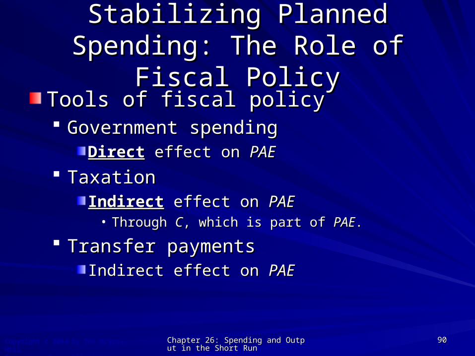
Tools of fiscal policyTools of fiscal policy Government spendingGovernment spending
DirectDirect effect on effect on PAEPAE
TaxationTaxationIndirectIndirect effect on effect on PAEPAE
• Through Through CC, which is part of , which is part of PAEPAE..
Transfer paymentsTransfer paymentsIndirect effect on Indirect effect on PAEPAE
Stabilizing Planned Spending: The Stabilizing Planned Spending: The Role of Fiscal PolicyRole of Fiscal Policy

Chapter 26: Spending and Output in theChapter 26: Spending and Output in the Short Run Short Run
9191Copyright c 2004 by The McGraw-HillCompanies, Inc. All rights reserved.
Pla
nn
ed a
gg
reg
ate
exp
end
itu
re P
AE
960
Expenditure line PAE = 960 + 0.8Y
E
An increase in G shifts the expenditure line upward
Output Y
Y = PAE
F
45o
4,800
Recessionary gap
Expenditure line PAE = 950 + 0.8Y
950
4,750
Y*
An Increase In Government An Increase In Government Purchases Eliminates A Recessionary GapPurchases Eliminates A Recessionary Gap

Chapter 26: Spending and Output in theChapter 26: Spending and Output in the Short Run Short Run
9292Copyright c 2004 by The McGraw-HillCompanies, Inc. All rights reserved.
Economic NaturalistEconomic Naturalist Why is Japan building roads nobody wants to Why is Japan building roads nobody wants to
use?use?Japan has a recessionary gapJapan has a recessionary gap
$1 trillion spending on public works$1 trillion spending on public works
The policy has not been successful to dateThe policy has not been successful to date• Was not large enoughWas not large enough• Wasteful spending may have demoralized consumersWasteful spending may have demoralized consumers
Stabilizing Planned Spending: The Stabilizing Planned Spending: The Role of Fiscal PolicyRole of Fiscal Policy
Chapter 26: Spending and Output in theChapter 26: Spending and Output in the Short Run Short Run
9393Copyright c 2004 by The McGraw-HillCompanies, Inc. All rights reserved.
Economic NaturalistEconomic Naturalist Does military spending stimulate the Does military spending stimulate the
economy?economy?
Stabilizing Planned Spending: The Stabilizing Planned Spending: The Role of Fiscal PolicyRole of Fiscal Policy
Chapter 26: Spending and Output in theChapter 26: Spending and Output in the Short Run Short Run
9494Copyright c 2004 by The McGraw-HillCompanies, Inc. All rights reserved.
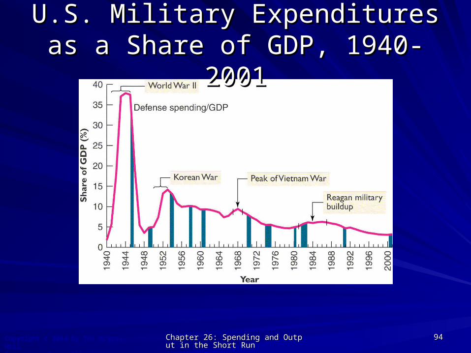
U.S. Military Expenditures as a U.S. Military Expenditures as a Share of GDP, 1940-2001Share of GDP, 1940-2001

Chapter 26: Spending and Output in theChapter 26: Spending and Output in the Short Run Short Run
9595Copyright c 2004 by The McGraw-HillCompanies, Inc. All rights reserved.
Taxes and Aggregate SpendingTaxes and Aggregate Spending Taxes affect Taxes affect PAEPAE indirectly indirectly Lower taxes increase Lower taxes increase disposable income (Y-T)disposable income (Y-T).. The Consumption Function isThe Consumption Function is
C=C+c(Y-T)C=C+c(Y-T) A tax A tax cutcut of X increases C by cX. of X increases C by cX. Therefore autonomous spending increases by Therefore autonomous spending increases by
cX when T falls by X.cX when T falls by X.cX < X.cX < X.
Stabilizing Planned Spending: The Stabilizing Planned Spending: The Role of Fiscal PolicyRole of Fiscal Policy
mpcT
C
Chapter 26: Spending and Output in theChapter 26: Spending and Output in the Short Run Short Run
9696Copyright c 2004 by The McGraw-HillCompanies, Inc. All rights reserved.
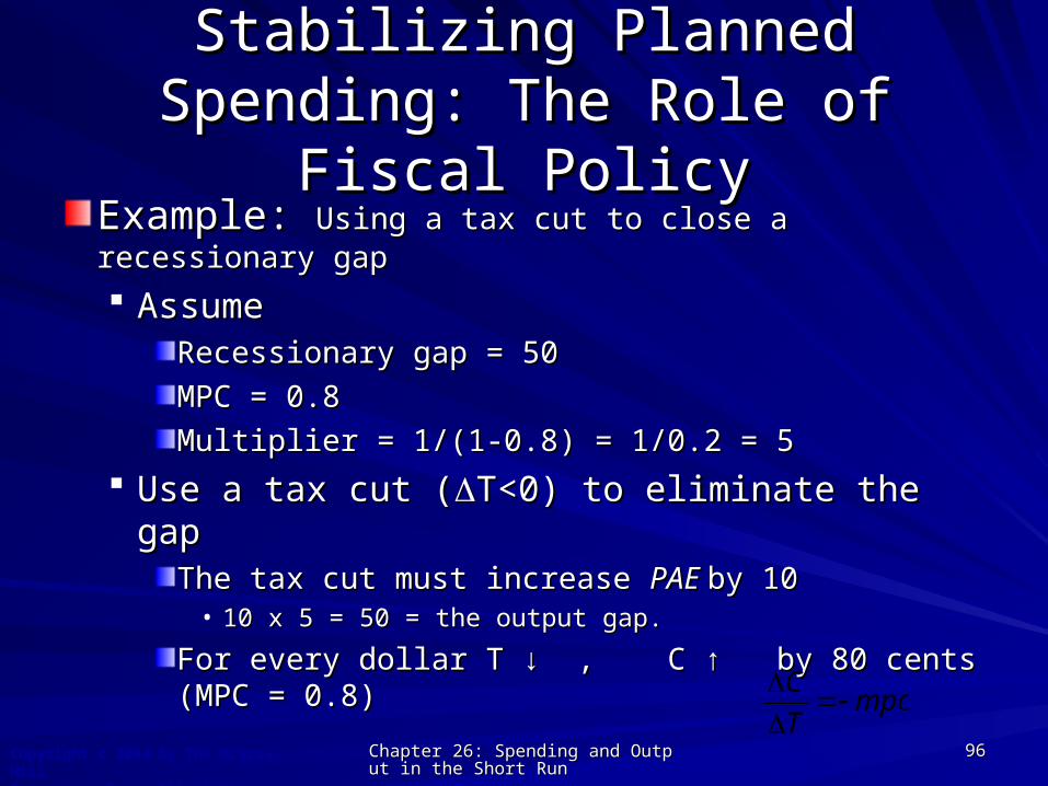
Example: Example: Using a tax cut to close a recessionary gapUsing a tax cut to close a recessionary gap
AssumeAssumeRecessionary gap = 50Recessionary gap = 50
MPC = 0.8MPC = 0.8
Multiplier = 1/(1-0.8) = 1/0.2 = 5Multiplier = 1/(1-0.8) = 1/0.2 = 5
Use a tax cut (Use a tax cut (T<0) to eliminate the gapT<0) to eliminate the gapThe tax cut must increase The tax cut must increase PAE PAE by 10by 10
• 10 x 5 = 50 = the output gap.10 x 5 = 50 = the output gap.
For every dollar T For every dollar T ↓↓ , C , C ↑ ↑ by 80 centsby 80 cents(MPC = 0.8)(MPC = 0.8)
Stabilizing Planned Spending: The Stabilizing Planned Spending: The Role of Fiscal PolicyRole of Fiscal Policy
mpcT
C

Chapter 26: Spending and Output in theChapter 26: Spending and Output in the Short Run Short Run
9797Copyright c 2004 by The McGraw-HillCompanies, Inc. All rights reserved.
ExampleExample Y* Y* –– Y = 50, multiplier = 5. Y = 50, multiplier = 5. The tax cut must cause The tax cut must cause C = 10.C = 10.
C = 10 = tax cut x MPC = tax cut x 0.8C = 10 = tax cut x MPC = tax cut x 0.8 Tax cut = Tax cut = C /MPC = 10/0.8 = 12.5C /MPC = 10/0.8 = 12.5
A tax cut of 12.5 increases C by 10 which A tax cut of 12.5 increases C by 10 which increases Y by 50.increases Y by 50.
Stabilizing Planned Spending: The Stabilizing Planned Spending: The Role of Fiscal PolicyRole of Fiscal Policy

Chapter 26: Spending and Output in theChapter 26: Spending and Output in the Short Run Short Run
9898Copyright c 2004 by The McGraw-HillCompanies, Inc. All rights reserved.
ExampleExample A tax cut of 12.5 increases C by 10 which A tax cut of 12.5 increases C by 10 which
increases Y by 50.increases Y by 50. What increase in G is necessary to achieve the What increase in G is necessary to achieve the
same increase in output?same increase in output? If the desired If the desired Y = 50 and the multiplier = 5,Y = 50 and the multiplier = 5,
G = 10.G = 10.
Stabilizing Planned Spending: The Stabilizing Planned Spending: The Role of Fiscal PolicyRole of Fiscal Policy
Multiplier =YY
autonomous AE)autonomous AE)
autonomous AE) autonomous AE) =YY
Multiplier
Chapter 26: Spending and Output in theChapter 26: Spending and Output in the Short Run Short Run
9999Copyright c 2004 by The McGraw-HillCompanies, Inc. All rights reserved.
Economic NaturalistEconomic Naturalist Why did the federal government send out Why did the federal government send out
millions of $300 and $600 checks to millions of $300 and $600 checks to households in 2001?households in 2001?
In the spring 2001, the U.S. economy was slowing.In the spring 2001, the U.S. economy was slowing.Summer 2001, families received $38 billion in tax Summer 2001, families received $38 billion in tax rebates.rebates.Survey indicated that only 22% of the households Survey indicated that only 22% of the households anticipated spending most of their rebates.anticipated spending most of their rebates.Tax cuts were accompanied by increases in Tax cuts were accompanied by increases in government spending to stimulate government spending to stimulate PAE.PAE.
Stabilizing Planned Spending: The Stabilizing Planned Spending: The Role of Fiscal PolicyRole of Fiscal Policy
Chapter 26: Spending and Output in theChapter 26: Spending and Output in the Short Run Short Run
100100Copyright c 2004 by The McGraw-HillCompanies, Inc. All rights reserved.
Fiscal Policy and Fiscal Policy and the Supply Sidethe Supply Side Fiscal policy may affect potential output as Fiscal policy may affect potential output as
well as well as PAE.PAE.Government spending and potential outputGovernment spending and potential output
• Public capitalPublic capital• R & DR & D• Human CapitalHuman Capital
Fiscal Policy as a Stabilization Fiscal Policy as a Stabilization Tool: Three QualificationsTool: Three Qualifications

Chapter 26: Spending and Output in theChapter 26: Spending and Output in the Short Run Short Run
101101Copyright c 2004 by The McGraw-HillCompanies, Inc. All rights reserved.
Fiscal Policy and the Supply SideFiscal Policy and the Supply Side Fiscal policy may affect potential output as Fiscal policy may affect potential output as
well as well as PAE.PAE.Taxation and potential outputTaxation and potential output
• Tax break for new investmentTax break for new investment• Tax break on interest income may stimulate savingTax break on interest income may stimulate saving• Tax break on income may stimulate more work.Tax break on income may stimulate more work.
Fiscal policy may affect both Fiscal policy may affect both PAE PAE and and Y*.Y*.
Fiscal Policy as a Stabilization Fiscal Policy as a Stabilization Tool: Three QualificationsTool: Three Qualifications

Chapter 26: Spending and Output in theChapter 26: Spending and Output in the Short Run Short Run
102102Copyright c 2004 by The McGraw-HillCompanies, Inc. All rights reserved.
The Problem of DeficitsThe Problem of Deficits Sustaining government deficits reduce saving Sustaining government deficits reduce saving
and investment in new capital goods.and investment in new capital goods.If a society has a goal of keeping deficits low, it If a society has a goal of keeping deficits low, it may have less of an incentive to use fiscal policy to may have less of an incentive to use fiscal policy to control a recessionary gap.control a recessionary gap.
Fiscal Policy as a Stabilization Fiscal Policy as a Stabilization Tool: Three QualificationsTool: Three Qualifications

Chapter 26: Spending and Output in theChapter 26: Spending and Output in the Short Run Short Run
103103Copyright c 2004 by The McGraw-HillCompanies, Inc. All rights reserved.
The The Relative InflexibilityRelative Inflexibility of Fiscal Policy of Fiscal Policy A lack of flexibility may reduce the A lack of flexibility may reduce the
effectiveness of fiscal policyeffectiveness of fiscal policy Two limits to fiscal policy flexibility:Two limits to fiscal policy flexibility:
The problem of time lags and the legislative The problem of time lags and the legislative processprocessCompeting political objectivesCompeting political objectives
Fiscal policy may be useful to address Fiscal policy may be useful to address prolonged periods of recession, but not to prolonged periods of recession, but not to “fine-tune” the economy.“fine-tune” the economy.
Fiscal Policy as a Stabilization Fiscal Policy as a Stabilization Tool: Three QualificationsTool: Three Qualifications
Chapter 26: Spending and Output in theChapter 26: Spending and Output in the Short Run Short Run
104104Copyright c 2004 by The McGraw-HillCompanies, Inc. All rights reserved.
Automatic stabilizers help offset the Automatic stabilizers help offset the inflexibility of fiscal policyinflexibility of fiscal policy Income tax collectionsIncome tax collections
Government takes in more money (automatically) Government takes in more money (automatically) when there is an expansionary gap.when there is an expansionary gap.
Suppose T = tY. Then Suppose T = tY. Then T = tT = tYY
Higher taxes reduce discretionary incomeHigher taxes reduce discretionary income(((Y(Y––T)=T)=––T), reducing autonomous expenditure T), reducing autonomous expenditure ((C=C=––ccT), and thus closing the expansionary T), and thus closing the expansionary gap.gap.
Fiscal Policy as a Stabilization Fiscal Policy as a Stabilization Tool: Three QualificationsTool: Three Qualifications
Chapter 26: Spending and Output in theChapter 26: Spending and Output in the Short Run Short Run
105105Copyright c 2004 by The McGraw-HillCompanies, Inc. All rights reserved.
What we’ve learnedWhat we’ve learned
Planned Aggregate ExpenditurePlanned Aggregate Expenditure= C + I= C + IPP + G + NX + G + NX
Actual expenditures may not equal Actual expenditures may not equal PAEPAE If so, unplanned inventory changes will occur.If so, unplanned inventory changes will occur. This will lead to changes in output and This will lead to changes in output and PAEPAE..
PAE depends positively on income.PAE depends positively on income. Higher income causes PAE to rise, but only Higher income causes PAE to rise, but only
by a proportion = by a proportion = mpc mpc < 1< 1..

Chapter 26: Spending and Output in theChapter 26: Spending and Output in the Short Run Short Run
106106Copyright c 2004 by The McGraw-HillCompanies, Inc. All rights reserved.
What we’ve learnedWhat we’ve learned
In the short run, planned aggregate In the short run, planned aggregate expenditures determine income and output.expenditures determine income and output.
Differences between PAE and Y cause Differences between PAE and Y cause unplanned changes in inventory, which unplanned changes in inventory, which cause output to change.cause output to change.
The process stopsThe process stopswhen PAE=Y.when PAE=Y.
Y
PAE

Chapter 26: Spending and Output in theChapter 26: Spending and Output in the Short Run Short Run
107107Copyright c 2004 by The McGraw-HillCompanies, Inc. All rights reserved.
What we’ve learnedWhat we’ve learned
Changes in autonomous PAE cause Changes in autonomous PAE cause changes in Y.changes in Y. The economicThe economic
process by which this happens is that as one process by which this happens is that as one person’s expenditures rise, someone else’s person’s expenditures rise, someone else’s income rise, raising his expenditure, etc.income rise, raising his expenditure, etc.
multipliermpcPAE
Y
1
1
0

Chapter 26: Spending and Output in theChapter 26: Spending and Output in the Short Run Short Run
109109Copyright c 2004 by The McGraw-HillCompanies, Inc. All rights reserved.
What we’ve learnedWhat we’ve learned
There’s no reason for short-run equilibrium There’s no reason for short-run equilibrium output to equal potential output.output to equal potential output. Potential output is determined by the productivity Potential output is determined by the productivity
and availability of labor, capital, etc.and availability of labor, capital, etc. Short-run equilibrium outputShort-run equilibrium output
is determined by plannedis determined by plannedaggregate expenditures.aggregate expenditures.
There’s no reason forThere’s no reason forthese two to be equal.these two to be equal.
Y Y*

Chapter 26: Spending and Output in theChapter 26: Spending and Output in the Short Run Short Run
110110Copyright c 2004 by The McGraw-HillCompanies, Inc. All rights reserved.
What we’ve learnedWhat we’ve learned
Fiscal policy (changes in G or T) can be Fiscal policy (changes in G or T) can be used to close output gaps.used to close output gaps. But it may respond slowly or inadequately.But it may respond slowly or inadequately.
Because there’s no reason for short-run Y to Because there’s no reason for short-run Y to be equal to Y*,be equal to Y*,
Governments can choose to intervene to Governments can choose to intervene to makemake them equal. them equal.
Chapter 26: Spending and Output in theChapter 26: Spending and Output in the Short Run Short Run
111111Copyright c 2004 by The McGraw-HillCompanies, Inc. All rights reserved.
In the long run, is he dead?In the long run, is he dead?