
Speeding up Martins’ algorithm for multiple objective ...
25
4OR manuscript No. (will be inserted by the editor) Speeding up Martins’ algorithm for multiple objective shortest path problems Sofie Demeyer · Jan Goedgebeur · Pieter Audenaert · Mario Pickavet · Piet Demeester Received: date / Accepted: date Abstract The latest transportation systems require the best routes in a large network with respect to multiple objectives simultaneously to be calculated in a very short time. The label setting algorithm of Martins efficiently finds this set of Pareto op- timal paths, but sometimes tends to be slow, especially for large networks such as transportation networks. In this article we investigate a number of speedup measures, resulting in new algorithms. It is shown that the calculation time to find the Pareto optimal set can be reduced considerably. Moreover, it is mathematically proven that these algorithms still produce the Pareto optimal set of paths. Keywords Multiobjective Shortest Path Problem · Labeling Algorithm · Stop Condition · Bidirectional Routing · Pareto Optimal Set Mathematics Subject Classification (2000) 90C29 · 05C85 · 05C38 · 68Q25 · 90B06 1 Introduction This paper presents two adaptations to a label setting algorithm, which was presented by Martins in 1984 [24], to solve the multiple objective shortest path problem. This is to date still a reference work to solve the multiple objective shortest path problem making use of graph algorithms. This section starts with a description of the problem tackled in this algorithm. Then an overview is given of what can be found in litera- ture about multiple objective shortest path problems and their solutions. Finally, the contributions and objectives of this research are explained. Dept. of Information Technology (INTEC), Ghent University - IBBT Gaston Crommenlaan 8/201, B-9050 Ghent Tel.: +32-9-331 49 77 Fax: +32-9-331 48 99 E-mail: sofi[email protected]
Transcript of Speeding up Martins’ algorithm for multiple objective ...

4OR manuscript No.(will be inserted by the editor)
Speeding up Martins’ algorithm for multiple objectiveshortest path problems
Sofie Demeyer · Jan Goedgebeur · PieterAudenaert · Mario Pickavet · Piet Demeester
Received: date / Accepted: date
Abstract The latest transportation systems require the best routes in a large networkwith respect to multiple objectives simultaneously to be calculated in a very shorttime. The label setting algorithm of Martins efficiently finds this set of Pareto op-timal paths, but sometimes tends to be slow, especially for large networks such astransportation networks. In this article we investigate a number of speedup measures,resulting in new algorithms. It is shown that the calculation time to find the Paretooptimal set can be reduced considerably. Moreover, it is mathematically proven thatthese algorithms still produce the Pareto optimal set of paths.
Keywords Multiobjective Shortest Path Problem · Labeling Algorithm · StopCondition · Bidirectional Routing · Pareto Optimal Set
Mathematics Subject Classification (2000) 90C29 · 05C85 · 05C38 · 68Q25 ·90B06
1 Introduction
This paper presents two adaptations to a label setting algorithm, which was presentedby Martins in 1984 [24], to solve the multiple objective shortest path problem. Thisis to date still a reference work to solve the multiple objective shortest path problemmaking use of graph algorithms. This section starts with a description of the problemtackled in this algorithm. Then an overview is given of what can be found in litera-ture about multiple objective shortest path problems and their solutions. Finally, thecontributions and objectives of this research are explained.
Dept. of Information Technology (INTEC), Ghent University - IBBT
Gaston Crommenlaan 8/201, B-9050 GhentTel.: +32-9-331 49 77Fax: +32-9-331 48 99E-mail: [email protected]
2 S. Demeyer et al.
1.1 Problem description
In this section, we present one of the possible applications of the research presentedin this article, namely routing in transportation networks.
With the evolvement of GPS systems, routing in transportation networks gainsmore attention. One of the main characteristics of these transportation networks isthat they tend to be large. For example the TIGER/Line network, covering the USA,consists of approximately 24 million nodes and 29 million links and the PTV Europenetwork contains approximately 19 million nodes and 23 million links [1]. In mostapplications, a preprocessing phase reduces the size of these networks, but even then,they are still extensive. On the other hand, these networks tend to be sparse with anaverage node degree between 2 and 3.
Moreover, in recent years, multimodal transportation (i.e. using multiple modes oftransportation) becomes a valuable alternative to avoid road traffic jams. Multimodalnetworks are often represented by a layered network model in which each modus hasits own transportation network and trans-shipments between the modes are modeledby trans-shipment links connecting nodes from different modes of transportation [9].This results in even more extensive networks than the unimodal ones.
At the same time, logistic applications need to find the best route as soon as pos-sible while taking into account multiple objectives. The transport needs to be both asfast, as cheap, as ecological, etc. as possible. The problem tackled in this article ishow to calculate in a very short time the multiple objective shortest paths between anorigin and a destination in a transportation network. As there are multiple objectivesthat need to be optimized, there is no single optimal path, but a set of paths that iscalled Pareto optimal. A path is called Pareto optimal if no objective can be ame-liorated without deteriorating another objective (see section 2.1 for a more formaldefinition).
For this, we will further improve the MOSP (multiple objective shortest path)algorithm of Martins, which has proven to be an efficient way to find the completePareto optimal set of paths [12], especially for lower density networks such as trans-portation networks. Unfortunately, this algorithm, in its original form, has to examinethe whole network to find the Pareto optimal set of routes. This is quite time consum-ing for large networks, such as (multimodal) transportation networks. Therefore, wewill attempt to limit the search area of the algorithm, namely by formulating a stopcondition to interrupt the search process and by searching the network bidirectionally(i.e. simultaneously from the origin and the destination).
In this article we assume that all objectives need to be minimized and all con-cepts are defined according to this assumption. Moreover, it should be noted that theresearch presented here assumes that all costs are non-negative and that there are nocycles with cost 0.
1.2 Literature overview
Multiple objective shortest path problems, which are known to be NP-hard [39],started to gain attention in the 70s and the beginning of the 80s with the works of
Speeding up Martins’ algorithm for MOSP 3
Vincke [43] and Hansen [21], in which they focused on the case with two objectives,the bi-objective shortest path problem. Since then, several exact methods, for boththe general multi-objective and the bi-objective shortest path problem, have been de-veloped to find all Pareto optimal paths between two nodes in a network.
The most straight-forward (and easiest) way to deal with multiple objectives ismaking use of single objective shortest path techniques with a weighted objectivefunction. Unfortunately, this method only finds a subset of all Pareto-optimal paths.If we present all Pareto-optimal paths in a decision space, the paths found by thisalgorithm are situated on the convex hull. The other Pareto-optimal paths are situ-ated in the so-called duality gaps. References [13] and [37] provide a more detaileddiscussion on this subject.
Exact methods to find the set of Pareto-optimal paths for the shortest path problemwith two objectives have been thoroughly studied. As we focus in this article on thegeneral multi-objective shortest path algorithm, we would just like to refer to theworks of Skriver [40] and Raith and Ehrgott [37] for an overview of most of thebi-objective shortest path algorithms.
In [7], Clımaco and Pascoal give an overview to solve the multi-objective shortestpath problems. According to the taxonomy presented in their article, the research pre-sented in this paper can be categorized in the class of multicriteria path problems withadditive metrics and a-posteriori aggregation of preferences method. In this class, twomajor categories can be distinguished: ranking techniques and labeling techniques.
Ranking techniques, like for example [6] and [2], use a ranking method for listingthe paths in a decreasing order according to one of the objectives. Subsequently, fromthis list of paths a set of non-dominated paths is determined. Three groups of pathranking methods can be determined: deletion algorithms ([25], [22], [29]) in whichat the start of each iteration the path found in the previous iteration is eliminatedfrom the network, labeling algorithms ([28], [26], [34]) in which nodes may containK labels (for the K paths) and that resemble the K shortest path algorithms, anddeviation algorithms ([23], [14], [27]) in which a new path is considered to be adeviation from the previous path.
Labeling techniques are well known to solve the single objective shortest pathproblem ([10], [3]). Similar to the single objective case, two categories can be dis-tinguished: label-setting algorithms and label-correcting algorithms. An exact label-setting algorithm for the bi-objective shortest path problem was proposed by Hansen[21]. This work was then generalized by Martins for the multiple objective shortestpath problem [24]. To this date, this article is still a reference work for the multi-objective shortest path algorithms.Next to label-setting algorithms, a number of label-correcting algorithms were presented. Similarly, this research started with bicriteriashortest path problems ([43], [5], [41]) and was then generalized for multiple crite-ria [38]. Guerriero and Musmanno studied the impact of label selection versus nodeselection in label-correcting algorithms [20]. For a detailed theoretical study of theproperties of label correcting and label setting algorithm to solve the multi-objectiveshortest path problem, we would like to refer to [30].
Most of the research described above assumes that all objectives are additive, butalso other objective types can be used. One of the most popular is a combination ofboth additive objectives and objectives of the bottleneck type (i.e. minmax, maxmin).

4 S. Demeyer et al.
Gandibleux et al. [16] generalized the algorithm of Martins to the case in which oneof the objectives is a bottleneck. In [8] and [35] an algorithm is presented to solve thetricriteria shortest path problem in which at least two objectives are of the bottlenecktype. A twofold extension to this latter research has been proposed by Bornstein etal. [4]. As we will focus on additive objectives in this research, we will not elaboratefurther on this.
Next to these exact methods, a number of well known heuristics have been ap-plied to the multi-objective shortest path problem. In [32], for example, evolutionaryalgorithms are used to find a subset of the Pareto optimal paths.
A complete overview of multiple objective shortest path algorithms, both for bi-criteria and multicriteria problems can be found in [17]. In this article we will focuson the exact label setting algorithm of Martins [24] with additive objectives, and pro-pose a number of adaptations to speed up the calculation in the case where we wantto find all non-dominated paths between a single origin node and a single destina-tion node. In the following section more details are given on the objectives and thecontributions that are made in this research.
1.3 Contributions and objectives
Our research focuses on exact and fast algorithms to solve multiple objective shortestpath problems with n objectives, which are all sum problems. This problem can bedescribed mathematically as
minp∈Ps,t (z1(p),z2(p), ...,zn(p))
in which Ps,t represents the set of all paths between a node s and a node t while zi(p) isthe cost of path p with respect to objective i. While some of the algorithms presentedin the literature are especially for the bicriterion problem ([40], [37]), we opted not tolimit the number of objectives (as for example in [20] and [38]). Moreover, we wantto speed up the calculations without losing the guarantee of finding all Pareto optimalpaths, in contrast with for example the heuristic search algorithm of [32].
This article focuses on two exact speedup techniques, namely a well-defined stopcondition and searching the network bidirectionally. It is shown that the two pro-posed improvements achieve a considerable speedup compared to other exact graphalgorithms, while at the same time maintaining the optimality of the solution.
In the first improvement a speedup is achieved by stopping the search as soonas all Pareto optimal paths between the origin and the destination are found, insteadof searching the whole network. The second one searches the network from both theorigin and the destination simultaneously, resulting in a speedup factor of more than2 (where the bidirectional algorithm of Dijkstra achieves a speedup factor of around2). This is clarified experimentally.
2 Unidirectional multiple objective shortest path algorithm
In order to better understand the remainder of the article, the unidirectional algo-rithm from which we started, is presented briefly in this section, together with a well-
Speeding up Martins’ algorithm for MOSP 5
defined stop condition that finishes the search process as soon as all Pareto optimalpaths are found. The first subsection discusses some basic (mathematical) conceptsthat are used by the algorithm. Subsequently, in the second subsection, the multi-ple objective shortest path algorithm is presented. In order to avoid investigating thewhole network, as the basic version of this algorithm does, a speedup can be achievedby making use of an efficient stop condition which is presented in subsection 2.3, to-gether with a proof of the correctness of this stop condition.
2.1 Basic concepts
A network is defined as a graph G(V,A) with V the set of nodes and A the set ofdirected links. Each link (x,y), connecting node x and node y, has assigned to it anumber of values representing the costs for the different objectives, which is repre-sented by a vector c(x,y) = [cxy1,cxy2, . . . ,cxyn]. In this paper we will assume that noparallel links are allowed. Nevertheless, parallel links would have no impact on theoperation of the algorithms presented here.
A path or a route in a graph is defined as a vector with a cost of the path forevery objective together with an ordered list of nodes, for which holds that each pairof consecutive nodes is connected by a link. So it can be represented as [c,P] withc = [c1,c2, . . . ,cn] = [ci] the cost vector and P = [v1, . . . ,vk] the ordered list of nodeswith ∀i ∈ {1, . . . ,k−1} : (vi,vi+1) ∈ A. Here the path contains k nodes and thus k−1links.
Similarly to the algorithm of Dijkstra [10], the algorithms presented in this arti-cle make use of labels to indicate the ‘distance’ to a certain node. A label containsa cost value for every objective and a reference to a previous label. In this way, alabel can be represented as L = [v, c,PrevL] with v the node to which this label isassigned, c = [c1,c2, . . . ,cn] the value vector and PrevL the reference to the previouslabel. The reference to the previous label enables reconstructing the path afterwardsby backtracking it. It should be noticed that, in this way, from every label a path canbe constructed. While in the algorithm of Dijkstra paths are reconstructed by back-tracking nodes, here this happens at label level.
In order to compare labels with each other, two relationships need to be definedon the cost vectors: dominance and ordering.
We will first define the dominance relationship between vectors in order to cometo a definition of Pareto optimality, as the result of the MOSP algorithm is a Paretooptimal set.
Definition 1 (dominance)The vector [a1, . . . ,an] dominates the vector [b1, . . . ,bn] if and only if
(∀i ∈ {1, . . . ,n} : ai ≤ bi)∧ (∃i ∈ {1, . . . ,n} : ai < bi)
A path P1 dominates another path P2 if and only if the cost vector of P1 dominates theone of P2.A label L1 dominates another label L2 if and only if the vector of L1 dominates theone of L2.

6 S. Demeyer et al.
Definition 2 (Pareto optimality)A path is Pareto optimal if and only if there exists no feasible path which is better inone of the objectives and not worse in all the other objectives.A set of paths S is called Pareto optimal if and only if none of the elements of S isdominated by another feasible path.
So, for example, if we have the paths A, B and C with cost vectors a = [5,9,3],b = [2,1,3] and c = [5,3,2] respectively, then A is dominated by both B and C. Thepaths B and C, on the other hand, form a set of Pareto optimal paths within the set{A,B,C}.
At certain points in the algorithm, the smallest/largest label needs to be deter-mined, so an ordering needs to be defined. We opted for a lexicographical orderingaccording to following definition.
Definition 3 (lexicographic ordering)The vector [a1, . . . ,an] is lexicographically smaller than (denoted by <l) the vec-
tor [b1, . . . ,bn] if and only if
∃k ∈ {1, . . . ,n} : (∀i < k : ai = bi)∧ (ak < bk)
A label L1 is lexicographically smaller than a label L2 if and only if the vector of L1is smaller than the one of L2
Now, if we want to order the vectors a, b and c, as presented previously, fromsmall to large then we get the sequence b <l c <l a.
This relationship is a total ordering relation, as it is reflexive, anti-symmetric andtransitive and two elements can always be compared to each other.
The lexicographic ordering is not the best ordering for multi-objective shortestpath algorithms. In [33] it is shown that a weighted sum aggregate ordering resultsin a remarkable reduction of the calculation time. Nevertheless, we opted for a lexi-cographic ordering as it is easy to incorporate and the aggregate ordering requires anormalization of the objectives (and according fine tuning of the parameters) whichmay differ from network to network.
2.2 The basic algorithm
The basic algorithm presented in this section is based on the multiple objective short-est path algorithm of Martins [24], which is, in turn, based on the algorithm of Dijk-stra [10]. Instead of only one label, nodes will now contain a set of labels. Moreover,this set only contains non-dominated labels. So, when adding a new label to a node,this label is only added when it is not dominated by one of the existing labels. More-over, labels that are dominated by the new label are removed from the set. Below thepseudo code of the algorithm is given, which calculates for every node of the networkthe set of Pareto optimal paths from a specific origin. For clarity reasons, an explana-tion of the pseudo code is given in table 1.
Algorithm 1
Speeding up Martins’ algorithm for MOSP 7
Table 1 Explanation of the pseudo code used in algorithm 1.
T the set of temporary labels[<node>,[v[1],...,v[n]],<label>] a label represented by its owner (node), a vector of
values (i.e. the cost of the path from the origin to thisnode) and the previous label
<node>.addLabel(<label>) adds a label to a node while removing all dominatedlabels
T.removeMin() removes the minimum label from T according to thelexicographic ordering
T.add(<label>) adds a label to the temporary set T<label>.owner() returns the node which is the owner of the label<node>.neighbors() returns the set of nodes which are adjacent to the nodegetLinkBetween(<node1>,<node2>) returns the link from node1 to node2[a[i]+b[i]] the pointwise sum of a and b. This is a short notation
for [a1 +b1, . . . ,an +bn]
T := EMPTYSET;
originLabel := [origin,[0,...,0],NULL];
origin.addLabel(originLabel);
T.add(originLabel);
while(T is not empty){label := T.removeMin();
owner := label.owner();
neighbours := owner.neighbours();
forall(nb in neighbors){link := getLinkBetween(owner, nb);
newLabel := [nb,[label[i]+link.cost[i]], label];
if(newLabel not dominated by any of nb.labels()){nb.addLabel(newLabel);
T.add(newLabel);
}}
}
Two phases can be distinguished: an initialization and the search phase. At ini-tialization all nodes have empty label sets, except for the origin node which con-tains the null label, i.e. a label containing the null vector and a null reference. Thislabel is added to the temporary set T . The algorithm runs until this temporary setis empty. At every iteration the minimum label, according to the lexicographic or-dering relationship, is determined and new labels are constructed for the neighborsof its owner (the owner of a label indicates the node which contains this label).[label[i] + link.cost[i]] denotes a vector which represents the pointwise sum of thevectors label and link.cost. If not dominated by any other, these new labels are addedto both the corresponding neighbor and the temporary set. Moreover, as a part of theaddLabel function, labels from the specific neighbor which are dominated by the newlabel are removed. If this new label is added to the label set of its owner, it is alsoadded to the temporary set.
8 S. Demeyer et al.
The main difference with the algorithm of Dijkstra is that this algorithm worksat label level instead of node level. The temporary set contains labels and instead ofchanging the label of a node, the Pareto optimal set of a node is altered by adding newlabels and removing dominated ones. Moreover, parents of labels are labels them-selves.
2.3 Stop condition
The algorithm presented in section 2.2 investigates the whole network in order tofind a set of Pareto optimal paths from one node to all others. In this research, we areinterested in all Pareto optimal paths between a single origin and a single destinationnode. Investigating the whole network then is superfluous as the Pareto optimal setis often already found before the algorithm terminated. In this section we presenta stop condition, which is similar to the one in [42], [11] and [36], also known as‘dominance by early results’ or multi-objective A*. The basic idea is that labels thatare dominated by one of the labels of the destination node can never lead to a Paretooptimal path, and thus are not worth investigating further. This follows from the factthat all costs are non-negative and the objectives are of the additive type.
In contrast with the multi-objective A* algorithm, we opted not to check thiscondition for every label when removed from the temporary set, but to keep trackof the minimum values for each objective of all labels present in the temporary setand check whether this vector is dominated by one of the destination labels. As thevector with the minimum values only differs little in each iteration, the number ofcomparison operations needed to check the dominance can be limited. This meansthat labels which are dominated by one of the result labels (i.e. the labels of thedestination node) may still be investigated, but this does not outweigh the smallernumber of comparison operations.
Assume [mini(T )] represents the pointwise minimum of every objective valueof all labels in T , resulting in the vector [min1(T ),min2(T ), . . . ,minn(T )]. It can beshown that if this minimum vector is dominated by any of the destination labels, thesearch can be finished.
Stop Condition 1 (unidirectional s-t algorithm)The search process can be stopped as soon as [mini(T )] is dominated by at least oneof the destination labels R ∈ Ldestination.
This can be proven (by contradiction) as follows.
Proof Assume that, once the stop condition holds, there still exists a label C withvector c = [ci] which is an element of the temporary set T and which is not dominatedby any of the destination labels. As this label is part of T :
ci ≥ mini(T ),∀i
The stop condition says that [min1(T ), . . . ,minn(T )] is dominated by at least one ofthe destination labels R = [destination, [ri],PrevR] ∈ Ldestination, which means that
mini(T )≥ ri,∀i
Speeding up Martins’ algorithm for MOSP 9
with at least one j for whichmin j(T )> r j
This results inci ≥ ri,∀i
with at least one j for whichc j > r j
According to the definition of dominance, this means that C is dominated by R, whichmeans that our initial assumption is false and that there exist no non-dominated labelsin T . ut
Applying this stop condition to the basic algorithm can easily be done by sub-stituting the line ’while(T is not empty)’ with ’while(T is not empty and
mini(T ) is not dominated by R in destination.labels())’
3 Bidirectional multiple objective shortest path algorithm
As searching the network bidirectionally has been proven useful when speeding upalgorithms, in this section a bidirectional multiple objective shortest path algorithmis presented, together with the proof that this algorithm always returns the Paretooptimal set of paths.
3.1 The algorithm
Multiple possibilities exist to speed up shortest path queries [15], like goal-directedsearch [19], bidirectional search [31], hierarchical search [18], etc. Some of themhave already been applied to the multi-objective shortest path problem, such as thegoal-directed (A*) algorithm of [42]. We opted to investigate the bidirectional speeduptechnique, as, with a well defined stop condition, this technique is able to guaranteestill finding the optimal path for single objective shortest path problems. The basicidea of a bidirectional shortest path algorithm is that the search procedure is dividedinto two separate procedures: a forward search starting from the origin node and abackward search starting from the destination node.
There are two factors that influence the efficiency of bidirectional shortest pathalgorithms, namely the alternation between the forward and the backward search andthe stop condition, of which the former is less critical than the latter. One can de-termine to alternate equally between the two searches or to pick the search directionwith the smallest label. In this research we opted to alternate equally, but this caneasily be changed.
The stop condition determines when it can be guaranteed that the optimal path hasbeen found, and thus when both searches can be interrupted. For the single objectiveshortest path search, it has been proven [31] that the shortest path is found once thecost of the shortest path found so far (i.e. the minimum sum of the forward and thebackward label of the same node) is smaller than or equal to the sum of the minimum
10 S. Demeyer et al.
labels of the forward and the backward temporary set. It should be noted that theperformance of the bidirectional shortest path algorithm (with the stop condition asmentioned before) is dependent upon the network configuration. Examples exist ofnetworks in which the two searches proceed in different directions, resulting in twonearly completely unidirectional search trees. Predicting the average speedup factorbased on qualitative or quantitative measures of the network is difficult. Nevertheless,for most planar and evenly distributed networks (i.e. networks in which the link costsare of the same magnitude), like the networks we are using in our research, a speedupof around 2 can be achieved.
The bidirectional multiple objective shortest path algorithm starts two search pro-cesses simultaneously: one from the origin and one from the destination. These searchprocesses are similar to the search process of the unidirectional algorithm, in whichnew labels are constructed for the neighbors of the owner of the investigated label.These new labels are then added to the (forward or backward) label set of the spe-cific nodes, if not dominated by any of the existing labels. Moreover, labels, whichare dominated by this new label, are removed from this set. It should be noticed thatnodes now contain two (Pareto optimal) label sets: one for the forward search andone for the backward search. When a new label is added to one of the label sets of anode and the other label set is not empty (i.e. this node has been visited in the otherdirection), this new label is combined with all labels of the other label set in order toform paths between the origin and the destination. These paths are then added to thetemporary Pareto optimal solution set. It should be noted that a path is represented bya cost vector, together with a description of the path itself (i.e. a list of nodes/links).However, in order to save memory space, in the implementation only the cost vectortogether with the forward and the backward label, that were combined, are stored inthe solution set. As each label contains a reference to its predecessor label, the pathcan be constructed from these two stored labels.
When all Pareto optimal paths are found both searches should be aborted. There-fore, a stop condition needs to be defined which guarantees that all Pareto optimalpaths are found. For this, we make use of the pointwise minima (defined as in sec-tion 2.3) [mini(TF)] and [mini(TB)] of the forward and the backward temporary setrespectively. A new label will be constructed which contains the pointwise sum ofthese minima [mini(TF)+mini(TB)] and this label will be compared to the paths ofthe solution set (R ∈ Lresult ). In the next section, it will be proven that the followingstop condition guarantees that all feasible Pareto optimal paths have been found.
Stop Condition 2 (bidirectional s-t algorithm)The forward and the backward search can be aborted when[mini(TF)+mini(TB)] is dominated by any of the result paths R ∈ Lresult .
Below, pseudo code of the bidirectional multiple objective algorithm is given.The code which has not been used in algorithm 1 is explained in table 2.
Algorithm 2
T[forward] := EMPTYSET;
T[backward] := EMPTYSET;
Speeding up Martins’ algorithm for MOSP 11
Table 2 Explanation of the pseudo code used in algorithm 2.
T[<direction>] the set of temporary labels in a specific directionL[result] the set of Pareto optimal (result) paths<node>.addLabel(<label>,<direction>) adds a label to a node in a specific direction while
removing all dominated labels in that direction<node>.labels(<direction>) returns the set of labels of a node in a specific direc-
tiongetDirection() determines in which direction the iteration of the al-
gorithm will take placed’ the opposite direction of dcombine(<label>, <set of labels>) combines the label with each of the elements of the
set to form a set of pathsLresult.addPaths(<set of paths>) adds all elements of the set to the result set, while
removing the dominated paths
Lresult := EMPTYSET;
originLabel := [origin,[0,...,0],NULL];
origin.addLabel(originLabel, forward);
T[forward].add(originLabel);
destinationLabel := [destination,[0,...,0],NULL];
destination.addLabel(destinationLabel, backward);
T[backward].add(destinationLabel);
while([mini(T[forward])+mini(T[backward])]
is not dominated by any R in Lresult){d := getDirection();
label := T[d].removeMin();
owner := label.owner();
neighbours := owner.neighbors();
forall(n in neighbors){link := getLinkBetween(owner, n);
newLabel := [n,[label[i]+link.cost[i]], label];
if(newLabel not dominated by any of n.labels(d)){n.addLabel(newLabel, d);
T[d].add(newLabel);
if(n.Labels(d’) is not empty){results := combine(newLabel, n.labels(d’));
Lresult.addResults(results);
}}
}}
First, both the forward and the backward temporary sets are initialized with anempty set. Similarly, the solution set Lresult is initialized. The temporary sets are or-
12 S. Demeyer et al.
dered according to the lexicographic ordering relationship, similar to the unidirec-tional algorithm. The solution set is a Pareto optimal set, which means that paths canbe added only if they are not dominated by any of the existing paths and that existingpaths which are dominated by the newly added path have to be removed from the set.Subsequently, a null label, i.e. a label containing the null vector and a null reference,is assigned to both the origin and the destination. The origin label is added to theforward temporary set, while the destination label is added to the backward set.
After initialization, the following steps are repeated until the stop condition (stopcondition 2) is met. First, a direction is determined. Multiple possibilities exist to dothis, like for example choosing the direction with the largest/smallest temporary setor alternating between the forward and the backward search. We opted for the latterone in order not to favor one of the directions. Then, the smallest label (according toa lexicographic ordering) is taken from the temporary set of the specific direction andinvestigated. This means that all neighbors of the owner of this label are determinedand new labels are constructed from the investigated label and the cost vectors ofthe links between this owner and its neighbors. Every new label then is added to thespecific (forward/backward) label set of the specific neighbor, if it is not dominatedby any of the existing labels of this set. When added successfully, all existing labelswhich are dominated by the new label are removed from the set and the new labelis added to the temporary set of the specific direction. Moreover, if this neighborcontains labels in the other direction d′ (i.e. the label set of the other direction is notempty), this new label is combined with each of the labels of the label set of the otherdirection in order to form new paths. These new paths are then added to the solutionset. It should be noted that this solution set is Pareto optimal, meaning that if the newpaths are dominated by one of the existing paths, they will not be added, and that, ifthey are added, all existing paths dominated by them will be eliminated.
This is repeated until the stop condition is met, which means that the label con-taining the pointwise sum of the pointwise minima of the temporary sets is dominatedby at least one of the resulting paths. These minima of the temporary sets are updatedevery time a new label is added to the set and every time a label is removed from it(when this label is investigated or when a temporary label is removed from a label setof a node).
This algorithm guarantees to find all Pareto optimal paths between the origin andthe destination, as will be shown in the next section.
3.2 Proof of the optimality
In this section we will prove the correctness of following theorem.
Theorem 1 (optimality bidirectional MOSP algorithm)All Pareto optimal paths are found once the stop condition holds for the bidirectionalmultiple objective shortest path algorithm.
Proof The bidirectional algorithm searches the network simultaneously from the ori-gin and the destination, similar to the search process of the unidirectional algorithm.When a node contains both forward and backward labels, these labels are combined

Speeding up Martins’ algorithm for MOSP 13
to form paths, which are then added to the solution set, if Pareto optimal. Once thestop condition holds, all forward labels XF with
∃i : xFi < mini(TF)
and all backward labels XB with
∃i : xBi < mini(TB)
have been investigated, i.e. they are permanent labels.This means that for all forward labels which have not been investigated yet holds that
∀i : xFi ≥ mini(TF) (1)
and for all uninvestigated backward labels
∀i : xBi ≥ mini(TB) (2)
The stop condition says that the pointwise sum of the pointwise minima of the tempo-rary sets is dominated by at least one path R = [[ri],PR] of the Pareto optimal solutionset Lresult , or
(∀i : mini(TF)+mini(Tb)≥ ri)∧ (∃i : mini(TF)+mini(Tb)> ri) (3)
Let us now assume that there still exists a path C = [[ci],PC], which has not beenfound yet, but should be an element of the solution set. This means that this path isnot dominated by any of the result paths R = [[ri],PR],R ∈ Lresult . According to thedominance definition, this implies that
∃i : ci < ri (4)
From the operation of bidirectional algorithm we know that this path C is constructedby combining two labels of the same node, namely CF and CB, thus
∀i : ci = cFi + cB
i (5)
Combining equations (3), (4) and (5) results in
∃i : cFi + cB
i < ri ≤ mini(TF)+mini(TB) (6)
or∃i : cF
i + cBi < mini(TF)+mini(TB) (7)
We will now demonstrate that this path C does not exist or that all paths for whichcondition (7) holds, have already been found by the algorithm. As path C has not beenfound yet, this means that either ∀i : cF
i ≥mini(TF) or ∀i : cBi ≥mini(TB) or both. This
latter case is in contradiction with comparison (7) and thus can never lead to a Paretooptimal path. Two possible situations remain, namely ∀i : cF
i ≥ mini(TF)∧ (∃i : cBi <
mini(TB)∨∀i : cBi = mini(TB)) and (∃i : cF
i < mini(TF)∨∀i : cFi = mini(TF))∧∀i :
cBi ≥mini(TB). Due to the symmetric character of the bidirectional algorithm we will

14 S. Demeyer et al.
only discuss one of these cases. The other one then can be deduced in the same way.Let us assume that
(∃i : cFi < mini(TF)∨∀i : cF
i = mini(TF))∧∀i : cBi ≥ mini(TB)
This means that the backward label has not been investigated yet, while the for-ward label is already made permanent. The investigated forward label implies thatall neighboring labels are already present in the network (some of them permanent,others not). If the path C has not been found yet by the algorithm, this means that thelabel CB is not yet present in the network.
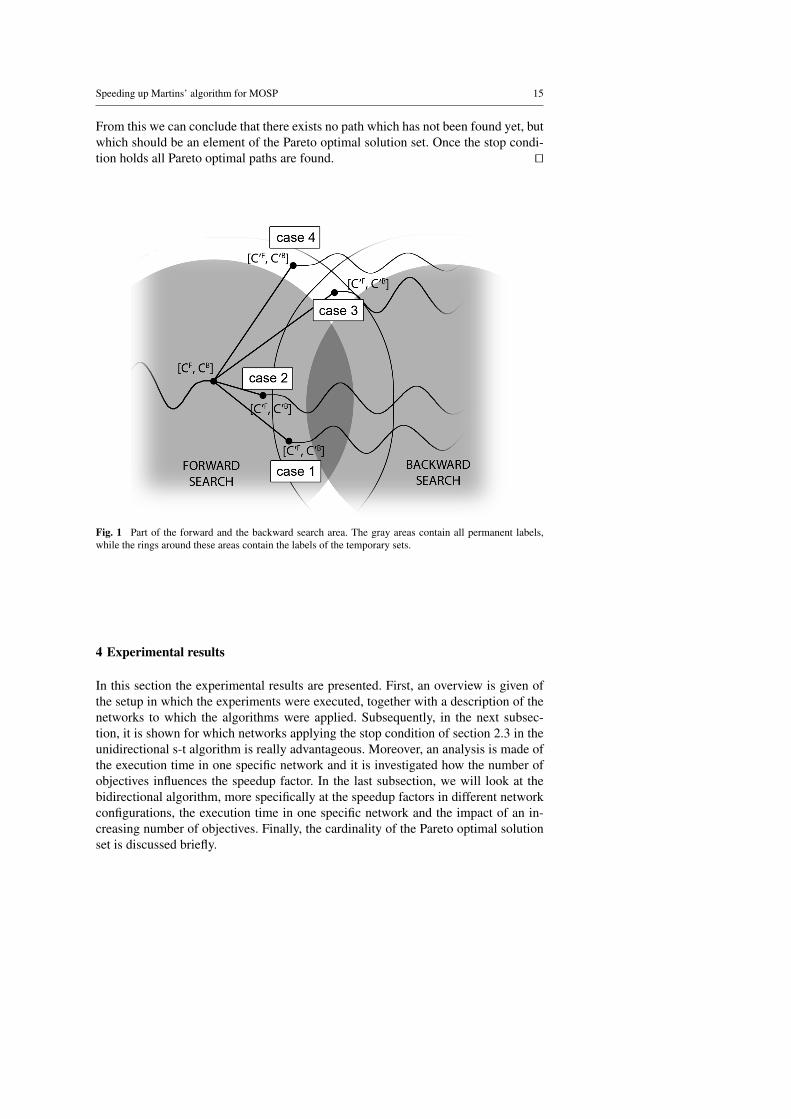
We will now look at the predecessor label C′B of this backward label CB. Let n′C bethe owner of this label C′B, while nC denotes the owner of the labels CF and CB. SinceCB and C′B are neighboring labels, the nodes nC and n′C are connected. Moreover, CF
is a permanent label, which implies that its neighboring labels are already present inthe network. From this, we can deduce that n′C contains a forward label C′F whichhas CF as predecessor label. All ‘labels’ can be divided into three subsets (areas) forboth the forward and the backward search: labels which have been investigated (i.e.permanent labels), labels which are added to a node but have not been investigatedyet (i.e. temporary labels) and labels which have not been found yet by the algorithm.We know that C′F is already present in the network, which means that it is eitherpermanent or temporary. Since label CB has not been found yet by the algorithm,label C′B has not been investigated yet, which means that is either a temporary labelor a label which has not been found yet. This leads to four cases for C′F and C′B asillustrated in figure 1.
Case 1: C′F is a permanent label and C′B is a temporary label. This path has beenfound by the algorithm as both the forward and the backward label are present in thenetwork.
Case 2: C′F is permanent and C′B is not an element of the backward search space(i.e has not been found yet). This means that
(∃i : c′Fi < mini(TF)∨∀i : c′Fi = mini(TF))∧∀i : c′Bi ≥ mini(TB)
which can be reduced to the initial situation by translating C′F and C′B to CF and CB
respectively.
Case 3: Both C′F and C′B are temporary labels. Similar to case 1, this path has beenfound since both the forward and the backward label are present in the network.
Case 4: C′F is an element of the forward temporary set and C′B has not been foundyet. As the label C′F is an element of the forward temporary set, this means that∀i : c′Fi ≥ mini(TF). Moreover, the label C′B is situated outside the backward searcharea, which means that ∀i : c′Bi ≥ mini(TB). Combining these labels will result in apath for which equation (7) does not hold and which thus cannot be an element of thePareto optimal set.
Speeding up Martins’ algorithm for MOSP 15
From this we can conclude that there exists no path which has not been found yet, butwhich should be an element of the Pareto optimal solution set. Once the stop condi-tion holds all Pareto optimal paths are found. ut
Fig. 1 Part of the forward and the backward search area. The gray areas contain all permanent labels,while the rings around these areas contain the labels of the temporary sets.
4 Experimental results
In this section the experimental results are presented. First, an overview is given ofthe setup in which the experiments were executed, together with a description of thenetworks to which the algorithms were applied. Subsequently, in the next subsec-tion, it is shown for which networks applying the stop condition of section 2.3 in theunidirectional s-t algorithm is really advantageous. Moreover, an analysis is made ofthe execution time in one specific network and it is investigated how the number ofobjectives influences the speedup factor. In the last subsection, we will look at thebidirectional algorithm, more specifically at the speedup factors in different networkconfigurations, the execution time in one specific network and the impact of an in-creasing number of objectives. Finally, the cardinality of the Pareto optimal solutionset is discussed briefly.
16 S. Demeyer et al.
4.1 Setup of the experiments
All algorithms presented in this paper were implemented in Java (version 1.6.0-18).We opted to represent the temporary set by a (lexicographically ordered) priorityqueue. Moreover, the label sets of the nodes were implemented as has hsets. Allexperiments were executed on a machine with the following configuration: Intel (R)Core(TM) 2 Duo CPU P8600, 2.40 GHz and 4 GB of RAM.
All graphs that are used in this research are assumed to be directed. All undirectedlinks were replaced by two inverse directed links. There are 4 network configurationsthat are used: transportation, square grid, random and complete networks.
A number of transportation networks (Transport X) were provided by a Belgiancompany who is a major industrial player in the field of traffic information. In thisresearch, we made use of a network representing the Belgian road network (B). More-over, the three transportation networks that were used in [36] and [37] were retrieved.These networks are road networks of the US, more specifically those of WashingtonDC (DC), Rhode Island (RI) and New Jersey (NJ). Next to the length of the links(i.e. streets, or part of streets), travel time information was made available. For theexperiments, the length (in meters) was utilized as first objective and the travel time(in milliseconds) as second objective. Since we do not have more data at hand, forthe other objectives random values between 0 and 1000 were used.
In a square grid network (Square Grid N) nodes are placed on a square grid (N ·N)and all the direct (horizontal and vertical) neighbors are connected to each other. Thismeans that each node has at most 4 neighbors. A grid network of this type is oftendenoted with the term ‘Manhattan network’. The cost vectors assigned to the linksconsist of n (assumed that there are n objectives) completely uncorrelated randomvalues between 0 and 1000.
A random network (Random N(d)) contains N nodes and (d ·N) links. Thesenodes are randomly connected to each other by the specified number of links, wherewe made sure that the networks are connected. This means that the network needs tocontain at least (N-1) links. Again, (completely uncorrelated) random values between0 and 1000 were used to represent the different costs of the links. Random networkshave the advantage that the number of nodes and the number of links can be changedeasily. In this research we will use the random networks to determine trends in thespeedup factors in function of the number of nodes in the networks and the averagenode degree in the networks.
Finally, a complete (or full dense) network (Complete N) is a network with Nnodes in which each node is connected to each of the other nodes. Here too, we madeuse of n completely uncorrelated random values (between 0 and 1000) to representthe cost vectors of the links.
An overview of all networks that were used in the experiments is given in table 3.All experiments were executed for 1000 randomly selected origin-destination
pairs and the presented results are averages over these 1000 multiple objective short-est path calculations. For both presented speedup techniques, speedup factors arereported, with a speedup factor (SUF) of algorithm A over algorithm B is defined as:
SUF(A/B) =avg. execution time algorithm Bavg. execution time algorithm A
Speeding up Martins’ algorithm for MOSP 17
Table 3 Overview of all network configurations used for the experiments.
network configuration # nodes # links averageoutdegree
Transport (DC) 9 559 29 765 3.1Transport (B) 23 080 50 364 2.2Transport (RI) 53 658 138 083 2.6Transport (NJ) 330 386 869 471 2.6Complete 100 100 9 900 99Complete 300 300 89 700 299Square Grid 30 900 3 480 3.86Square Grid 100 10 000 39 600 3.96Random 10000(3) 10 000 30 000 3Random 20000(3) 20 000 60 000 3Random 100000(3) 100 000 300 000 3Random 10000(4) 10 000 40 000 4Random 10000(5) 10 000 50 000 5Random 10000(6) 10 000 60 000 6
A speedup factor higher than 1 means that algorithm A is faster than algorithm B.For clarity issues, we will denote the unidirectional MOSP algorithm without thestop condition with U, the unidirectional MOSP algorithm with the stop conditionwith US and the bidirectional MOSP algorithm (with the stop condition) with B.
4.2 The unidirectional MOSP algorithm
In this section we will demonstrate that using the stop condition (see section 2.3) in-deed speeds up a number of unidirectional shortest path calculations in some networkconfigurations. In the first part a comparison will be made of the speedup factors forthe different network configurations. Subsequently, we will look at one specific con-figuration and see how the calculation time varies with a varying ‘distance’ betweenthe origin and the destination.
Table 4 shows the average execution time of the unidirectional MOSP algo-rithm without the stop condition and the speedup achieved by using stop condition1 (SUF(US/U)) for a number of network configurations, and this for both 2 and 3objectives. One can see that the speedup factors for the transportation networks aremuch higher than those for the other networks. The results for the three US network(DC, RI and NJ) are comparable to the results of [36]. For the square grid networks,on the other hand, slightly higher speedup factors are perceived. Applying the stopcondition in a complete network does not result in smaller execution times. At alltimes, the whole network needs to be investigated and the algorithm with the stopcondition is even slightly slower than the algorithm without the stop condition, dueto the overhead of checking the stop condition. Looking at the random networks,two trends are perceived. When the number of nodes in the network increases, thespeedup factor increases as well. The larger the network is, the higher the chance thatthe origin and the destination node are ‘closer’ to each other and that only a smallerpart of the network needs to be investigated. If the number of nodes in the network iskept constant and the average out degree of the nodes is increased, the speedup factor
18 S. Demeyer et al.
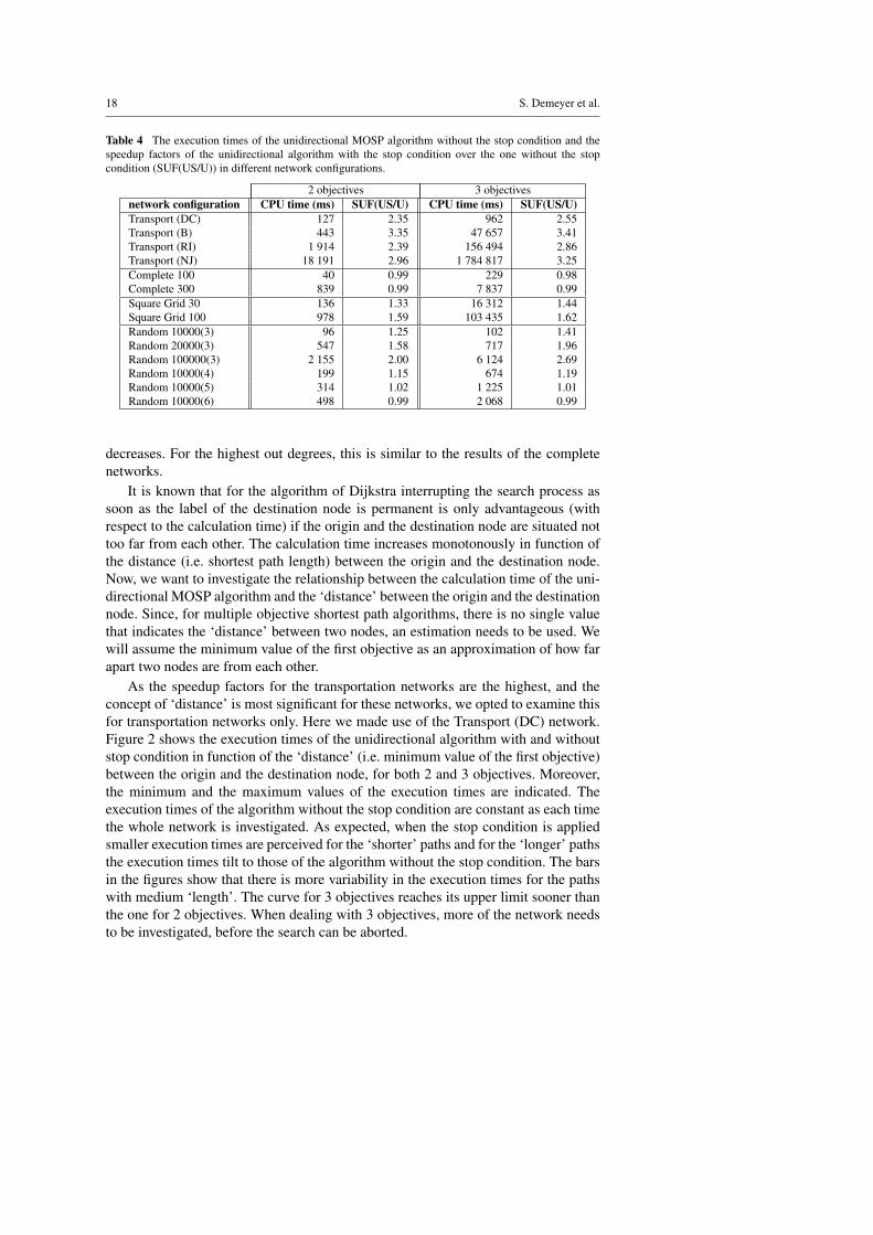
Table 4 The execution times of the unidirectional MOSP algorithm without the stop condition and thespeedup factors of the unidirectional algorithm with the stop condition over the one without the stopcondition (SUF(US/U)) in different network configurations.
2 objectives 3 objectivesnetwork configuration CPU time (ms) SUF(US/U) CPU time (ms) SUF(US/U)Transport (DC) 127 2.35 962 2.55Transport (B) 443 3.35 47 657 3.41Transport (RI) 1 914 2.39 156 494 2.86Transport (NJ) 18 191 2.96 1 784 817 3.25Complete 100 40 0.99 229 0.98Complete 300 839 0.99 7 837 0.99Square Grid 30 136 1.33 16 312 1.44Square Grid 100 978 1.59 103 435 1.62Random 10000(3) 96 1.25 102 1.41Random 20000(3) 547 1.58 717 1.96Random 100000(3) 2 155 2.00 6 124 2.69Random 10000(4) 199 1.15 674 1.19Random 10000(5) 314 1.02 1 225 1.01Random 10000(6) 498 0.99 2 068 0.99
decreases. For the highest out degrees, this is similar to the results of the completenetworks.
It is known that for the algorithm of Dijkstra interrupting the search process assoon as the label of the destination node is permanent is only advantageous (withrespect to the calculation time) if the origin and the destination node are situated nottoo far from each other. The calculation time increases monotonously in function ofthe distance (i.e. shortest path length) between the origin and the destination node.Now, we want to investigate the relationship between the calculation time of the uni-directional MOSP algorithm and the ‘distance’ between the origin and the destinationnode. Since, for multiple objective shortest path algorithms, there is no single valuethat indicates the ‘distance’ between two nodes, an estimation needs to be used. Wewill assume the minimum value of the first objective as an approximation of how farapart two nodes are from each other.
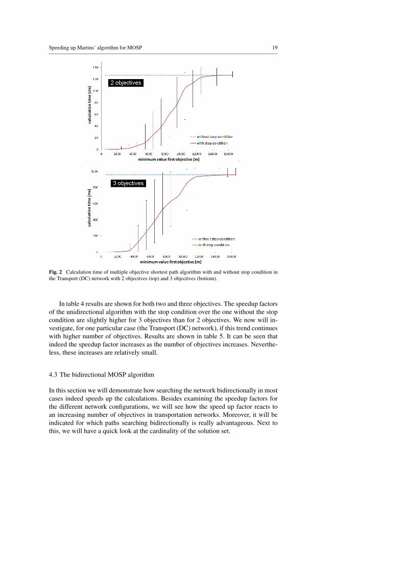
As the speedup factors for the transportation networks are the highest, and theconcept of ‘distance’ is most significant for these networks, we opted to examine thisfor transportation networks only. Here we made use of the Transport (DC) network.Figure 2 shows the execution times of the unidirectional algorithm with and withoutstop condition in function of the ‘distance’ (i.e. minimum value of the first objective)between the origin and the destination node, for both 2 and 3 objectives. Moreover,the minimum and the maximum values of the execution times are indicated. Theexecution times of the algorithm without the stop condition are constant as each timethe whole network is investigated. As expected, when the stop condition is appliedsmaller execution times are perceived for the ‘shorter’ paths and for the ‘longer’ pathsthe execution times tilt to those of the algorithm without the stop condition. The barsin the figures show that there is more variability in the execution times for the pathswith medium ‘length’. The curve for 3 objectives reaches its upper limit sooner thanthe one for 2 objectives. When dealing with 3 objectives, more of the network needsto be investigated, before the search can be aborted.
Speeding up Martins’ algorithm for MOSP 19
Fig. 2 Calculation time of multiple objective shortest path algorithm with and without stop condition inthe Transport (DC) network with 2 objectives (top) and 3 objectives (bottom).
In table 4 results are shown for both two and three objectives. The speedup factorsof the unidirectional algorithm with the stop condition over the one without the stopcondition are slightly higher for 3 objectives than for 2 objectives. We now will in-vestigate, for one particular case (the Transport (DC) network), if this trend continueswith higher number of objectives. Results are shown in table 5. It can be seen thatindeed the speedup factor increases as the number of objectives increases. Neverthe-less, these increases are relatively small.
4.3 The bidirectional MOSP algorithm
In this section we will demonstrate how searching the network bidirectionally in mostcases indeed speeds up the calculations. Besides examining the speedup factors forthe different network configurations, we will see how the speed up factor reacts toan increasing number of objectives in transportation networks. Moreover, it will beindicated for which paths searching bidirectionally is really advantageous. Next tothis, we will have a quick look at the cardinality of the solution set.

20 S. Demeyer et al.
Table 5 Speedup factors (SUF) of the unidirectional MOSP algorithm for different number of objectivesin the Transport(DC) network.
# obj. SUF(US/U)2 2.353 2.554 2.695 2.766 2.877 2.978 3.05
Table 6 The average execution times of the unidirectional MOSP algorithm with the stop condition andthe speedup factors of the bidirectional algorithm over the unidirectional algorithm with the stop condition(SUF(B/US)) in different network configurations.
2 objectives 3 objectivesnetwork configuration CPU time (ms) SUF(B/US) CPU time (ms) SUF(B/US)Transport (DC) 54 5.76 377 12.47Transport (B) 132 5.91 13 976 14.46Transport (RI) 801 7.77 54 718 16.16Transport (NJ) 6 146 10.08 549 174 21.43Complete 100 40 0.60 305 0.50Complete 300 847 0.58 7 916 0.37Square Grid 30 102 1.49 11 328 1.57Square Grid 100 615 1.79 63 849 1.96Random 10000(3) 77 3.29 72 3.54Random 20000(3) 346 3.99 66 3.99Random 100000(3) 1 078 4.52 2 277 4.67Random 10000(4) 173 2.75 566 2.51Random 10000(5) 308 2.01 1 213 1.30Random 10000(6) 503 1.04 2 89 0.53
Table 6 shows, next to the average cardinality of the solution set, the speedupfactors of the bidirectional MOSP algorithm over the unidirectional algorithm withthe stop condition, for both 2 and 3 objectives. Clearly noticeable is the fact that thespeedup factors in the transportation networks are higher than those in the other net-work configurations. Searching the network bidirectionally is certainly not a goodchoice when dealing with complete networks. Here, the bidirectional algorithm iseven slower than its unidirectional counterpart. For square grid networks, only rel-atively small speedups are achieved. Looking at the random networks, some trendscan be identified. When the number of nodes in the network increases, the speedupfactor increases too. If, on the other hand, the number of nodes is kept constant, andthe average out degree of the nodes is increased, the speedup factor decreases. Thesetrends are similar to the ones observed for the speedup factor of the unidirectionalalgorithm with the stop condition over the one without the stop condition.
Similar to the results of section 4.2 we looked at the calculation time of the bidi-rectional MOSP algorithm in the Transport (DC) network in function of the ‘dis-tance’ (i.e. minimum value of the first objective) between the origin and the desti-nation node. This is shown in figure 3, together with the calculation time of the uni-directional algorithm with the stop condition, which is the same as in figure 2. One

Speeding up Martins’ algorithm for MOSP 21
Fig. 3 Comparison of unidirectional and bidirectional algorithm in function of the number of hops in theshortest path.
can see that the calculation times for the bidirectional algorithm are indeed muchsmaller. The curves of the bidirectional algorithm increase monotonously, seeminglywithout reaching an upper limit, like the curves of the unidirectional algorithms do.This means that the highest speedups are achieved for the medium length paths. Forthe shortest paths the curves are nearly flat for both algorithms, resulting in smallerspeedup factors. When the ‘distance’ between the origin and the destination node in-creases, the calculation time of the unidirectional algorithm increases faster than thatof the bidirectional algorithm. This results in higher speedup factors. For the longestpaths the unidirectional algorithm has reached its upper limit, while the calculationtime of the bidirectional algorithm still increases, resulting in smaller speedup factors.So, the highest speedup factors are calculated for the medium length paths.
Subsequently, we investigated the impact of the number of objectives on thespeedup factor. In table 6 results are shown for both 2 and 3 objectives, where it can
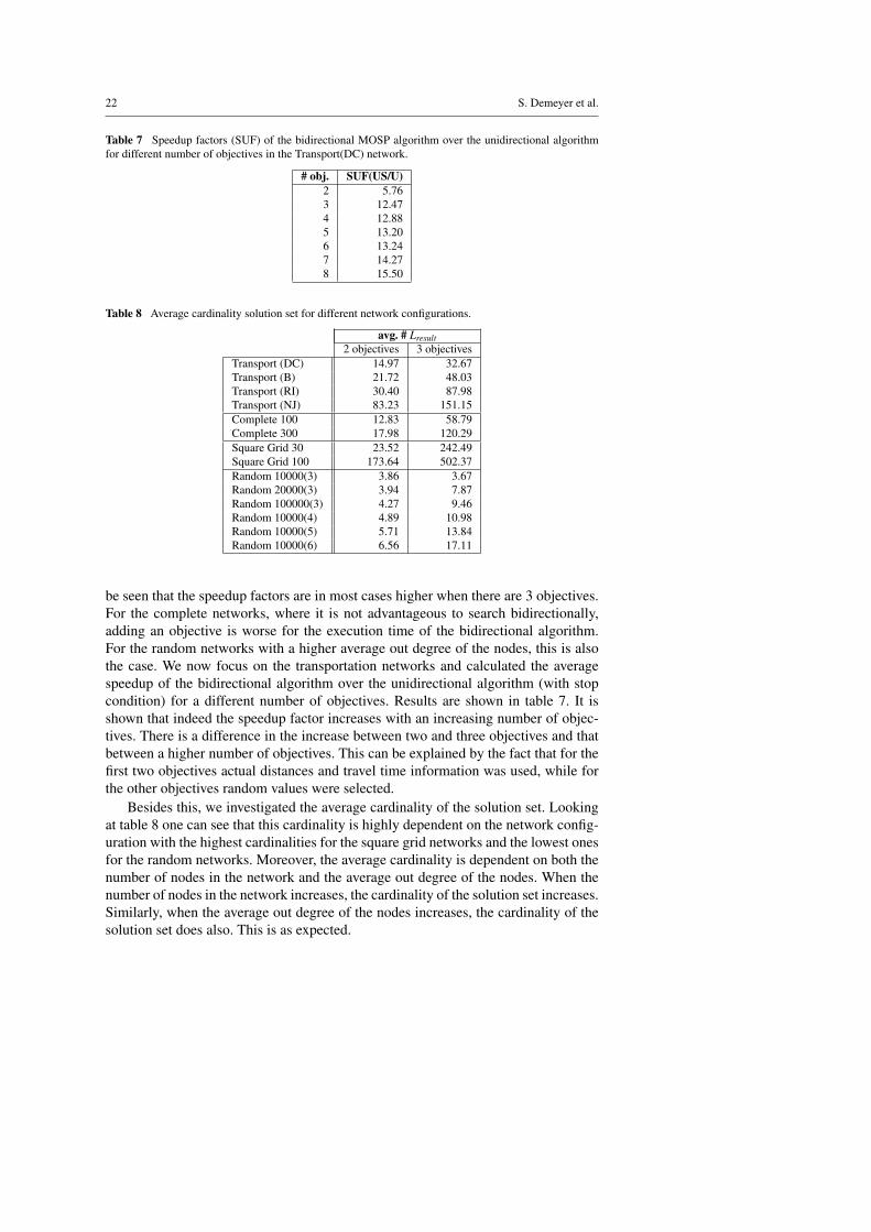
22 S. Demeyer et al.
Table 7 Speedup factors (SUF) of the bidirectional MOSP algorithm over the unidirectional algorithmfor different number of objectives in the Transport(DC) network.
# obj. SUF(US/U)2 5.763 12.474 12.885 13.206 13.247 14.278 15.50
Table 8 Average cardinality solution set for different network configurations.
avg. # Lresult2 objectives 3 objectives
Transport (DC) 14.97 32.67Transport (B) 21.72 48.03Transport (RI) 30.40 87.98Transport (NJ) 83.23 151.15Complete 100 12.83 58.79Complete 300 17.98 120.29Square Grid 30 23.52 242.49Square Grid 100 173.64 502.37Random 10000(3) 3.86 3.67Random 20000(3) 3.94 7.87Random 100000(3) 4.27 9.46Random 10000(4) 4.89 10.98Random 10000(5) 5.71 13.84Random 10000(6) 6.56 17.11
be seen that the speedup factors are in most cases higher when there are 3 objectives.For the complete networks, where it is not advantageous to search bidirectionally,adding an objective is worse for the execution time of the bidirectional algorithm.For the random networks with a higher average out degree of the nodes, this is alsothe case. We now focus on the transportation networks and calculated the averagespeedup of the bidirectional algorithm over the unidirectional algorithm (with stopcondition) for a different number of objectives. Results are shown in table 7. It isshown that indeed the speedup factor increases with an increasing number of objec-tives. There is a difference in the increase between two and three objectives and thatbetween a higher number of objectives. This can be explained by the fact that for thefirst two objectives actual distances and travel time information was used, while forthe other objectives random values were selected.
Besides this, we investigated the average cardinality of the solution set. Lookingat table 8 one can see that this cardinality is highly dependent on the network config-uration with the highest cardinalities for the square grid networks and the lowest onesfor the random networks. Moreover, the average cardinality is dependent on both thenumber of nodes in the network and the average out degree of the nodes. When thenumber of nodes in the network increases, the cardinality of the solution set increases.Similarly, when the average out degree of the nodes increases, the cardinality of thesolution set does also. This is as expected.
Speeding up Martins’ algorithm for MOSP 23
5 Conclusion
In this article the main goal was to speed up the multiple objective shortest path(MOSP) algorithm as presented by Martins [24], while still maintaining the guaranteeto find all Pareto optimal paths. The improvements prove to be very useful, especiallyin large transportation networks.
First, a stop criterion for the unidirectional algorithm was introduced which fin-ishes the search process as soon as the destination node contains all its labels, whichcan be translated to the Pareto optimal paths. It has been proven that, once this stopcondition holds, all Pareto optimal paths are found. Experiments have shown that aremarkable speedup can be achieved in transportation networks and that this speedupis the largest if the origin and the destination node are ‘close’ to each other. Moreover,the speedup factor increases when dealing with more objectives.
Secondly, a bidirectional MOSP algorithm was introduced, which searches thenetwork from the origin and the destination simultaneously. It is proven that thisalgorithm always returns the complete Pareto optimal set of paths. In the experiments,it can be seen that the speedup achieved by searching the network bidirectionally isdependent upon the network configuration, the number of nodes in the network, theaverage out degree of the nodes, the relative position of the origin and the destinationnode, and the number of objectives.
From the experiments it can be concluded that the speedup measures presented inthis article are particularly well suited for (large) transportation networks. The highestspeedup is achieved by searching the network bidirectionally.
References
1. 9th DIMACS Implementation Challenge: Shortest Paths, http://www.dis.uniroma1.it/∼challenge9(2006)
2. Azevedo JA., Costa MEOS., Madeira JJERS., Martins EQV., An algorithm for the ranking of shortestpaths, European Journal of Operational Research, 69, 97-106 (1993)
3. Bellman R., On a Routing Problem, Quarterly of Applied Mathematics, 16, 87-90 (1958)4. Bornstein C., Maculan N., Pascoal MMB., Pinto L., Multiobjective combinatorial optimization prob-
lems with a cost and several bottleneck objective functions: an algorithm with reoptimization, Com-puters & Operations Research, 39, 1969-1976 (2012)
5. Brumbaugh-Smith J., Shier D., An empirical investigation of some bicriterion shortest path algo-rithms, European Journal of Operational Research, 43, 216-224 (1989)
6. Clımaco JNC., Martins EQV., A bicriterion shortest path algorithm, European Journal of OperationalResearch, 11, 399-404 (1982)
7. Clımaco JNC., Pascoal MMB., Multicriteria path and tree problems - Discussion on exact algorithmsand applications, International Transactions in Operations Research, 19, 63-98 (2012)
8. de Lima Pinto L., Bornstein CT., Maculan N., The tricriterion shortest path problem with at least twobottleneck objective functions, European Journal of Operational Research, 198, 387-391 (2009)
9. Demeyer S., Audenaert P., Slock B., Pickavet M., Demeester P. Multimodal transport planning ina dynamic environment, Conference on Intelligent Public Transport Systems, Amsterdam, 155-167(2008)
10. Dijkstra EW., A Note on Two Problems in Connexion with Graphs, Numerische Mathematik, 1, 269-271 (1959)
11. Disser Y., Muller-Hannemann M., Schnee M., Multi-Criteria Shortest Paths in Time-Dependent TrainNetworks, Experimental Algorithms, 7th International Workshop, WEA 2008, Provincetown, MA,USA, 2008, 347-361 (2008)

24 S. Demeyer et al.
12. Ehrgott M., Gandibleux X., A survey and annotated bibliography of multiobjective combinatorialoptimization, OR Spektrum, 22, 425-460 (2000)
13. Ehrgott M., Gandibleux X., Multiple Criteria Optimization: State of the Art Annotated BibliographicSurveys, International Series in Operations Research and Management Science, 52, Springer (2002)
14. Eppstein D., Finding the k shortest paths. SIAM Journal on Computing, 28, 652-673 (1998)15. Fu L., Sun D., Rilett LR., Heuristic shortest path algorithms for transportation applications: State of
the art, Computers and Operations Research, 33, 3324-3343 (2006)16. Gandibleux X., Beugnies F., Randriamasy S., Martins’ algorithm revisited for multi-objective shortest
path problems with MaxMin cost function, 4OR - a Quarterly Journal for Operations Research, 4, 47-59 (2006)
17. Garroppo RG., Giordano S., Tavanti L., A survey on multi-constrained optimal path computation:Exact and approximate algorithms, Computer Networks, 54, 3081-3107 (2010)
18. Geisberger R., Sanders P., Schultes D., Delling D., Contraction Hierarchies: Faster and Simpler Hi-erarchical Routing in Road Networks, in: McGeoch (Ed.): Workshop on Experimental Algorithms,LNCS 5038, Springer-Verlag, Berlin/Heidelberg, 319-333 (2008)
19. Goldberg A., Kaplan H.,Werneck R., Reach for A*: Efficient point-to-point shortest path algorithms,in: Workshop on Algorithm Engineering & Experiments, Miami, 129-143 (2006)
20. Guerriero F., Musmanno R., Label Correcting Methods to Solve Multicriteria Shortest Path Problems,Journal of Optimization Theory and Applications, 111, 589-613 (2001)
21. Hansen P., Bicriterion path problems, in: Fandel G, Gal T (Eds), Multiple Criteria Decision Making:Theory and Applications, Lecture Notes in Economics and in Mathematical Systems 177, Springer:Heidelberg, 109-127 (1980)
22. Jimenez V., Marzal A., Computing the K shortest paths: a new algorithm and experimental compari-son, in: Vitter JS. Zaroliagis CD. (eds) Proceedings of the 3rd International Workshop on AlgorithmEngineering, LNCS 1668, Springer-Verlag, Berlin/Heidelberg, 15-29 (1999)
23. Jimenez V., Marzal A., A lazy version of Eppstein’s k shortest path algorithm, in: Jansen K., MargrafM., Matrolli M., Rolim J. (eds) Proceedings of the 2nd International Workshop on Experimental andEfficient Algorithms, LNCS 2647, Springer-Verlag, Berlin/Heidelberg, 179-191 (2003)
24. Martins EQV., On a multicriteria shortest path problem, European Journal of Operational Research,16, 236-245 (1984)
25. Martins EQV., An algorithm for ranking paths that may contain cycles, European Journal of Opera-tional Research, 18, 123-130 (1984)
26. Martins EQV., Paixao JM., Rosa MS., Santos JLE., Ranking multiobjective shortest paths, Pre-publicacoes do Departamento de Matematica 07-11, Universidade de Coimbra (2007)
27. Martins EQV., Pascoal MMB., Santos JLE., Deviation algorithms for ranking shortest paths. TheInternational Journal of Foundations of Computer Science, 10, 247-263 (1999)
28. Martins EQV., Pascoal MMB., Santos JLE., Labeling algorithms for ranking shortest paths. TechnicalReport 001 CISUC (2000)
29. Martins EQV., Pascoal MMB., Santos JLE., A new improvement for a K shortest path algorithm.Investigacao Operational, 21, 47-60 (2001)
30. Martins EQV., Santos JLE., The Labeling Algorithm for the Multiobjective Shortest Path Problem,CISUC Technical Report TR 99/005, University of Coimbra, Portugal (1999)
31. Nicholson JAT., Finding the shortest route between two points in a network. Computer Journal, 9,275-280 (1966)
32. Pangilinan JMA., Janssens GK., Evolutionary Algorithms for the Multiobjective Shortest Path Prob-lem, International Journal of Applied Science, Engineering and Technology, 4, 205-210 (2007)
33. Paixao JM., Santos JL., Labelling methods for the general case of the multi-objective shortest pathproblem - a computational study, Pre-publicacoes do Departamento de Matematica 07-42, Universi-dade de Coimbra (2007)
34. Paixao JM., Santos JL., A new ranking path algorithm for the multiobjective shortest path problem,Pre-publicacoes do Departamento de Matematica 08-27, Universidade de Coimbra (2008)
35. Pinto L., Pascoal MMB., On algorithms for tricriteria shortest path problems with two bottleneckobjective functions, Computers & Operations Research, 37, 1774-1779 (2010)
36. Raith A., Speed-up of labelling algorithms for biobjective shortest path problems, Proceedings of the45th Annual Conference of the ORSNZ, Auckland, New Zealand, 313-322 (2010)
37. Raith A., Ehrgott M., A comparison of solution strategies for biobjective shortest path problems,Computers & Operations Research, 36, 1299-1331 (2009)
38. Sastry V., Janakiraman T., Mohideen S., New algorithms for multi-objective shortest path problem,Opsearch, 40, 278-298 (2003)

Speeding up Martins’ algorithm for MOSP 25
39. Serafini P., Some considerations about computational complexity for multiobjective combinatorialproblems, Recent advances and historical development of vector optimization, 294, 222-232 (1986)
40. Skriver AJV., A classification of bicriterion shortest path (BSP) algorithms, Asia Pacific Journal ofOperational Research, 17, 192-212 (2000)
41. Skriver AJV., Andersen K., A label correcting approach for solving bicriterion shortest-path problems,Computers & Operations Research, 27, 507-524 (2000)
42. Stewart BS., White CC., Multiobjective A*, Journal of the Association for Computing Machinery, 38,775-814 (1991)
43. Vincke P., Problemes multicriteres, Cahiers Centre Etudes Recherche Operationnelle, 16, 425-439(1974)


![Bio-Inspired Source Seeking: A Hybrid Speeding up and ...C66]AKCDC16.pdf · Bio Inspired Source Seeking: a Hybrid Speeding Up and Slowing Down Algorithm* Ayesha Khan 1,Vivek Mishra](https://static.fdocuments.in/doc/165x107/5f9ee10fdf76af141553511c/bio-inspired-source-seeking-a-hybrid-speeding-up-and-c66akcdc16pdf-bio.jpg)