JADERBERG, VEDALDI, ZISSERMAN: SPEEDING UP CONVOLUTIONAL NEURAL... 1

Speeding up Convolutional Neural Networks

with Low Rank Expansions

Max Jaderbergmax@robots.ox.ac.uk

Andrea Vedaldivedaldi@robots.ox.ac.uk

Andrew Zissermanaz@robots.ox.ac.uk

Visual Geometry GroupDepartment of Engineering ScienceUniversity of OxfordOxford, UK

Abstract

The focus of this paper is speeding up the application of convolutional neural net-works. While delivering impressive results across a range of computer vision and ma-chine learning tasks, these networks are computationally demanding, limiting their de-ployability. Convolutional layers generally consume the bulk of the processing time, andso in this work we present two simple schemes for drastically speeding up these layers.This is achieved by exploiting cross-channel or filter redundancy to construct a low rankbasis of filters that are rank-1 in the spatial domain. Our methods are architecture ag-nostic, and can be easily applied to existing CPU and GPU convolutional frameworksfor tuneable speedup performance. We demonstrate this with a real world network de-signed for scene text character recognition [15], showing a possible 2.5⇥ speedup withno loss in accuracy, and 4.5⇥ speedup with less than 1% drop in accuracy, still achievingstate-of-the-art on standard benchmarks.

1 IntroductionMany applications of machine learning, and most recently computer vision, have been dis-rupted by the use of convolutional neural networks (CNNs). The combination of an end-to-end learning system with minimal need for human design decisions, and the ability toefficiently train large and complex models, have allowed them to achieve state-of-the-artperformance in a number of benchmarks [10, 14, 19, 33, 37, 38]. However, these high per-forming CNNs come with a large computational cost due to the use of chains of severalconvolutional layers, often requiring implementations on GPUs [16, 19] or highly optimizeddistributed CPU architectures [40] to process large datasets. The increasing use of these net-works for detection in sliding window approaches [9, 28, 33] and the desire to apply CNNsin real-world systems means the speed of inference becomes an important factor for appli-cations. In this paper we introduce an easy-to-implement method for significantly speedingup pre-trained CNNs requiring minimal modifications to existing frameworks. There canbe a small associated loss in performance, but this is tunable to a desired accuracy level.For example, we show that a 4.5⇥ speedup can still give state-of-the-art performance in ourexample application of character recognition.

c� 2014. The copyright of this document resides with its authors.It may be distributed unchanged freely in print or electronic forms.

2 JADERBERG, VEDALDI, ZISSERMAN: SPEEDING UP CONVOLUTIONAL NEURAL...

While a few other CNN acceleration methods exist, our key insight is to exploit theredundancy that exists between different feature channels and filters [6]. We contributetwo approximation schemes to do so (Sect. 2) and two optimization methods for each scheme(Sect. 2.2). Both schemes are orthogonal to other architecture-specific optimizations and canbe easily applied to existing CPU and GPU software. Performance is evaluated empiricallyin Sect. 3 and results are summarized in Sect. 4.

Related work. There are only a few general speedup methods for CNNs. Denton et al. [7]use low rank approximations and clustering of filters achieving 1.6⇥ speedup of single con-volutional layers (not of the whole network) with a 1% drop in classification accuracy. Ma-malet et al. [22] design the network to use rank-1 filters from the outset and combine themwith an average pooling layer; however, the technique cannot be applied to general networkdesigns. Vanhoucke et al. [40] show that 8-bit quantization of the layer weights can result ina speedup with minimal loss of accuracy. Not specific to CNNs, Rigamonti et al. [32] showthat multiple image filters can be approximated by a shared set of separable (rank-1) filters,allowing large speedups with minimal loss in accuracy. We build on this approach in ourwork.

Moving to hardware-specific optimizations, cuda-convnet [19] and Caffe [16]show that highly optimized CPU and GPU code can give superior computational perfor-mance in CNNs. [23] performs convolutions in the Fourier domain through FFTs computedefficiently over batches of images on a GPU. Other methods from [40] show that specificCPU architectures can be taken advantage of, e.g. by using SSSE3 and SSSE4 fixed-pointinstructions and appropriate alignment of data in memory. Farabet et al. [8] show that usingbespoke FPGA implementations of CNNs can greatly increase processing speed.

To speed up test-time in a sliding window context for a CNN, [13] shows that multi-scalefeatures can be computed efficiently by simply convolving the CNN across a flattened multi-scale pyramid. Furthermore, search space reduction techniques such as selective search [39]drastically cut down the number of times a full forward pass of the CNN must be computedby cheaply identifying a small number of candidate object locations in the image.

Note, the methods we propose are not specific to any processing architecture and can becombined with many of the other speedup methods given above.

2 Filter Approximations

Filter banks are used widely in computer vision as a method of feature extraction, and whenused in a convolutional manner, generate feature maps from input images. For an inputx 2 RH⇥W , the set of output feature maps Y = {y1,y2, . . . ,yN}, yn 2 RH 0⇥W 0 are generatedby convolving x with N filters F = { fi} 8i 2 [1 . . .N] such that yi = fi ⇤ x. The collectionof filters F can be learnt, for example, through dictionary learning methods [18, 20, 31] orCNNs, and are generally full rank and expensive to convolve with large images. Using adirect implementation of convolution, the complexity of convolving a single channel inputimage with a bank of N 2D filters of size d ⇥ d is O(d2NH 0W 0). We next introduce ourmethod for accelerating this computation that takes advantage of the fact that there existssignificant redundancy between different filters and feature channels.

One way to exploit this redundancy is to approximate the filter set by a linear combinationof a smaller basis set of M filters [32, 35, 36]. The basis filter set S= {si} 8i2 [1 . . .M] is usedto generate basis feature maps which are then linearly combined such that yi ' ÂM

k=1 aiksk ⇤x.

JADERBERG, VEDALDI, ZISSERMAN: SPEEDING UP CONVOLUTIONAL NEURAL... 3

This can lead to a speedup in feature map computation as a smaller number of filters need beconvolved with the input image, and the final feature maps are composed of a cheap linearcombination of these. The complexity in this case is O((d2M +MN)H 0W 0), so a speedupcan be achieved if M < d2N

d2+N .As shown in Rigomonti et al. [32], further speedups can be achieved by choosing the

filters in the approximating basis to be rank-1 and so making individual convolutions sepa-rable. This means that each basis filter can be decomposed in to a sequence of horizontaland vertical filters si ⇤ x = vi ⇤ (hi ⇤ x) where si 2 Rd⇥d , vi 2 Rd⇥1, and hi 2 R1⇥d . Usingthis decomposition, the convolution of a separable filter si can be performed in O(2dH 0W 0)operations instead of O(d2H 0W 0).

The separable filters of [32] are a low-rank approximation, but performed in the spatialfilter dimensions. Our key insight is that in CNNs substantial speedups can be achievedby also exploiting the cross-channel redundancy to perform low-rank decomposition in thechannel dimension as well. We explore both of these low-rank approximations in the sequel.

Note that the FFT [23] could be used as an alternative speedup method to accelerate indi-vidual convolutions in combination with our low-rank cross-channel decomposition scheme.However, separable convolutions have several practical advantages: they are significantlyeasier to implement than a well tuned FFT implementation, particularly on GPUs; they donot require feature maps to be padded to a special size, such as a power of two as in [23];they are far more memory efficient; and, they yield a good speedup for small image and filtersizes too (which can be common in CNNs), whilst FFT acceleration tends to be better forlarge filters due to the overheads incurred in computing the FFTs.

2.1 Approximating Convolutional Neural Network Filter Banks

CNNs are obtained by stacking multiple layers of convolutional filter banks on top of eachother, followed by a non-linear response function. Each filter bank or convolutional layertakes an input which is a feature map zi(u,v) where (u,v) 2 Wi are spatial coordinates andzi(u,v) 2RC contains C scalar features or channels zc

i (u,v). The output is a new feature mapzi+1 2 RH 0⇥W 0⇥N such that zn

i+1 = hi(Win ⇤ zi + bin) 8n 2 [1 . . .N], where Win and bin denotethe n-th filter kernel and bias respectively, and hi is a non-linear activation function such asthe Rectified Linear Unit (ReLU) hi(z) =max{0,z}. Convolutional layers can be intertwinedwith normalization, subsampling, and pooling layers which build translation invariance inlocal neighbourhoods. Other layer types are possible as well, but generally the convolutionalones are the most expensive. The process starts with z1 = x, where x is the input image, andends by, for example, connecting the last feature map to a logistic regressor in the case ofclassification. All the parameters of the model are jointly optimized to minimize a loss overthe training set using Stochastic Gradient Descent (SGD) with back-propagation.

The N filters Wn learnt for each layer (for convenience we drop the layer subscript i) arefull rank, 3D filters with the same depth as the number of channels of the input, such thatWn(u,v) 2 RC. For example, for a 3-channel color image input, C = 3. The convolutionWn ⇤ z of a 3D filter Wn with the 3D image z is the 2D image Wn ⇤ z = ÂC

c=1 W cn ⇤ zc, where

W cn 2Rd⇥d is a single channel of the filter. This is a sum of 2D convolutions so we can think

of each 3D filter as being a collection of 2D filters, whose output is collapsed to a 2D signal.However, since N such 3D filters are applied to z, the overall output is a new 3D image withN channels. This process is illustrated for the case C = 1,N > 1 in Fig. 1 (a). The resultingcomputational cost for a convolutional layer with N filters of size d ⇥ d acting on C input

4 JADERBERG, VEDALDI, ZISSERMAN: SPEEDING UP CONVOLUTIONAL NEURAL...

(a) (b)

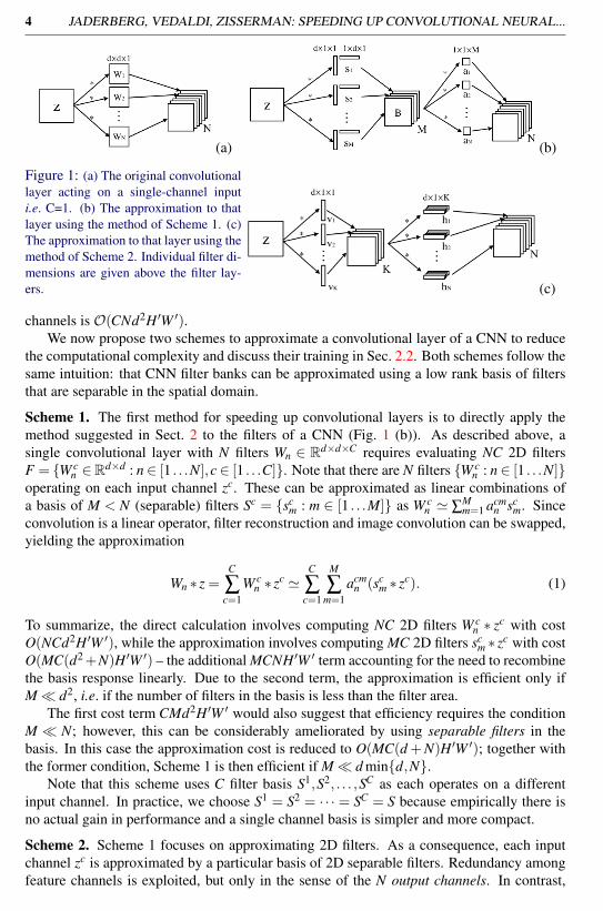
Figure 1: (a) The original convolutionallayer acting on a single-channel inputi.e. C=1. (b) The approximation to thatlayer using the method of Scheme 1. (c)The approximation to that layer using themethod of Scheme 2. Individual filter di-mensions are given above the filter lay-ers. (c)

channels is O(CNd2H 0W 0).We now propose two schemes to approximate a convolutional layer of a CNN to reduce

the computational complexity and discuss their training in Sec. 2.2. Both schemes follow thesame intuition: that CNN filter banks can be approximated using a low rank basis of filtersthat are separable in the spatial domain.

Scheme 1. The first method for speeding up convolutional layers is to directly apply themethod suggested in Sect. 2 to the filters of a CNN (Fig. 1 (b)). As described above, asingle convolutional layer with N filters Wn 2 Rd⇥d⇥C requires evaluating NC 2D filtersF = {W c

n 2Rd⇥d : n 2 [1 . . .N],c 2 [1 . . .C]}. Note that there are N filters {W cn : n 2 [1 . . .N]}

operating on each input channel zc. These can be approximated as linear combinations ofa basis of M < N (separable) filters Sc = {sc

m : m 2 [1 . . .M]} as W cn ' ÂM

m=1 acmn sc

m. Sinceconvolution is a linear operator, filter reconstruction and image convolution can be swapped,yielding the approximation

Wn ⇤ z =C

Âc=1

W cn ⇤ zc '

C

Âc=1

M

Âm=1

acmn (sc

m ⇤ zc). (1)

To summarize, the direct calculation involves computing NC 2D filters W cn ⇤ zc with cost

O(NCd2H 0W 0), while the approximation involves computing MC 2D filters scm ⇤ zc with cost

O(MC(d2+N)H 0W 0) – the additional MCNH 0W 0 term accounting for the need to recombinethe basis response linearly. Due to the second term, the approximation is efficient only ifM ⌧ d2, i.e. if the number of filters in the basis is less than the filter area.

The first cost term CMd2H 0W 0 would also suggest that efficiency requires the conditionM ⌧ N; however, this can be considerably ameliorated by using separable filters in thebasis. In this case the approximation cost is reduced to O(MC(d +N)H 0W 0); together withthe former condition, Scheme 1 is then efficient if M ⌧ d min{d,N}.

Note that this scheme uses C filter basis S1,S2, . . . ,SC as each operates on a differentinput channel. In practice, we choose S1 = S2 = · · · = SC = S because empirically there isno actual gain in performance and a single channel basis is simpler and more compact.

Scheme 2. Scheme 1 focuses on approximating 2D filters. As a consequence, each inputchannel zc is approximated by a particular basis of 2D separable filters. Redundancy amongfeature channels is exploited, but only in the sense of the N output channels. In contrast,

JADERBERG, VEDALDI, ZISSERMAN: SPEEDING UP CONVOLUTIONAL NEURAL... 5

Scheme 2 is designed to take advantage of both input and output redundancies by considering3D filters throughout. The idea is simple: each convolutional layer is factored as a sequenceof two regular convolutional layers but with rectangular (in the spatial domain) filters, asshown in Fig. 1 (c). The first convolutional layer has K filters of spatial size d ⇥1 resultingin a filter bank {vk 2 Rd⇥1⇥C : k 2 [1 . . .K]} and producing output feature maps V such thatV (u,v) 2 RK . The second convolutional layer has N filters of spatial size 1⇥d resulting ina filter bank {hn 2 R1⇥d⇥K : n 2 [1 . . .N]}. Differently from Scheme 1, the filters operate onmultiple channels simultaneously. The rectangular shape of the filters is selected to match aseparable filter approximation. To see this, note that convolution by one of the original filtersWn ⇤ z = ÂC

c=1 W cn ⇤ zc is approximated by

Wn⇤z' hn⇤V =K

Âk=1

hkn⇤V k =

K

Âk=1

hkn⇤(vk ⇤z) =

K

Âk=1

hkn⇤

C

Âc=1

vck ⇤zc =

C

Âc=1

"K

Âk=1

hkn ⇤ vc

k

#⇤zc (2)

which is the sum of separable filters hkn ⇤ vc

k. The computational cost of this scheme isO(KCdH 0W ) for the first vertical filters and O(NKdH 0W 0) for the second horizontal fil-ter. Assuming that the image width W � d is significantly larger than the filter size, theoutput image width W ⇡W 0 is about the same as the input image width W 0. Hence the totalcost can be simplified to O(K(N +C)dH 0W 0). Compared to the direct convolution cost ofO(NCd2H 0W 0), this scheme is therefore convenient provided that K(N +C) ⌧ NCd. Forexample, if K, N, and C are of the same order, the speedup is about d times.

In both schemes, we are assuming that the full rank original convolutional filter bank canbe decomposed into a linear combination of a set of separable basis filters. The differencebetween the schemes is how/where they model the interaction between input and outputchannels, which amounts to how the low rank channel space approximation is modelled. InScheme 1 it is done with the linear combination layer, whereas with Scheme 2 the channelinteraction is modelled with 3D vertical and horizontal filters inducing a summation overchannels as part of the convolution.

2.2 OptimizationThis section deals with the details on how to attain the optimal separable basis representationof a convolutional layer for the schemes. The first method (Sec. 2.2.1) aims to reconstructthe original filters directly by minimizing filter reconstruction error. The second method(Sec. 2.2.2) approximates the convolutional layer indirectly, by minimizing the empiricalreconstruction error of the filter output.

2.2.1 Filter Reconstruction Optimization

The first way that we can attain the separable basis representation is to aim to minimize thereconstruction error of the original filters with our new representation.

Scheme 1. The separable basis can be learnt simply by minimizing the L2 reconstructionerror of the original filters, whilst penalizing the nuclear norm ksmk⇤ of the filters sm. In fact,the nuclear norm ksmk⇤ is a proxy for the rank of sm 2Rd⇥d and rank-1 filters are separable.This yields the formulation:

min{sm},{an}

N

Ân=1

C

Âc=1

�����W cn �

M

Âm=1

acmn sm

�����

2

2

+lM

Âm=1

ksmk⇤. (3)

6 JADERBERG, VEDALDI, ZISSERMAN: SPEEDING UP CONVOLUTIONAL NEURAL...

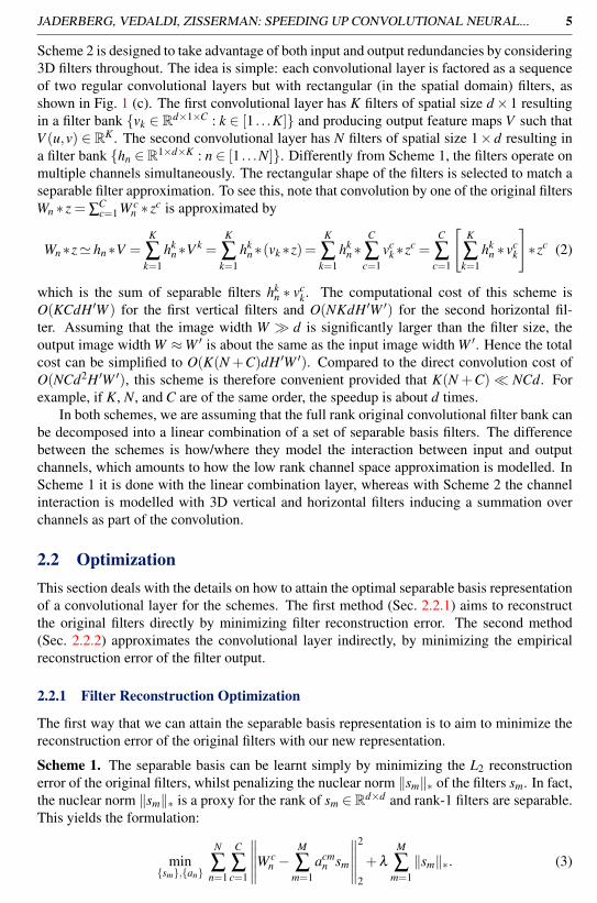
(a) (b)Figure 2: Example network schematics of how to optimize separable basis approximation layers in adata reconstruction setting. (a) Approximating Conv2 with Sep2. (b) Approximating Conv3 with Sep3,incorporating the approximation of Conv2 as well. Conv2 and Conv3 represent the original full-rankconvolutional layers, whereas Sep2 and Sep3 represent the approximation structure that is learnt byback-propagating the L2 error between the outputs.

This minimization is biconvex, so given sm a unique an can be found, therefore a minimum isfound by alternating between optimizing sm and an. A suitably large l ensures the resultingfilters are rank-1. For full details of the implementation of this optimization see [32].

Scheme 2. The set of horizontal and vertical filters can be learnt by explicitly minimizingthe L2 reconstruction error of the original filters. From (2) we can see that the original filtercan be approximated by minimizing the objective function

min{hk

n},{vck}

N

Ân=1

C

Âc=1

�����W cn �

K

Âk=1

hkn ⇤ vc

k

�����

2

2

. (4)

This optimization is simpler than for Scheme 1 due to the lack of nuclear norm constraints,which we are able to avoid by modelling the separability explicitly with two variables. Weperform conjugate gradient descent, alternating between optimizing the horizontal and ver-tical filter sets.

2.2.2 Data Reconstruction Optimization

The problem with optimizing the separable basis through minimizing original filter recon-struction error is that this does not necessarily give the most optimized basis set for the endCNN prediction performance. As an alternative, one can optimize a scheme’s separable basisby aiming to reconstruct the outputs of the original convolutional layer given training data.For example, for Scheme 2 this amounts to

min{hk

n},{vck}

|X |Âi=1

N

Ân=1

�����Wn ⇤Fl�1(xi)�C

Âc=1

K

Âk=1

hkn ⇤ vc

k ⇤Fl�1(xi)

�����

2

2

(5)

where l is the index of the convolutional layer to be approximated and Fl(xi) is the evaluationof the CNN up to and including layer l on data sample xi 2 X where X is the set of trainingexamples. This optimization can be done quite elegantly by simply mirroring the CNNwith the un-optimized separable basis layers, and training only the approximation layer byback-propagating the L2 error between the output of the original layer and the output of theapproximation layer (see Fig. 2). This is done layer by layer.

There are two main advantages of this method for optimization of the approximationschemes. The first is that the approximation is conditioned on the manifold of the trainingdata – original filter dimensions that are not relevant or redundant in the context of the train-ing data will by ignored by minimizing data reconstruction error, but will still be penalisedby minimizing filter reconstruction error (Sec. 2.2.1) and therefore uselessly using up model

JADERBERG, VEDALDI, ZISSERMAN: SPEEDING UP CONVOLUTIONAL NEURAL... 7

Layer name Filter size In channels Out channels Filters Maxout groups TimeConv1 9⇥9 1 48 96 2 0.473ms (8.3%)Conv2 9⇥9 48 64 128 2 3.008ms (52.9%)Conv3 8⇥8 64 128 512 4 2.160ms (38.0%)Conv4 1⇥1 128 37 148 4 0.041ms (0.7%)

Softmax - 37 37 - - 0.004ms (0.1%)

Table 1: The details of the layers in the CNN used with the forward pass timings of each layer.

capacity. Secondly, stacks of approximated layers can be learnt to incorporate the approxi-mation error of previous layers by feeding the data through the approximated net up to layerl rather than the original net up to layer l (see Fig. 2 (b)). This additionally means that all theapproximation layers could be optimized jointly with back-propagation.

An obvious alternative optimization strategy would be to replace the original convo-lutional layers with the un-optimized approximation layers and train just those layers byback-propagating the classification error of the approximated CNN. However, this does notactually result in better classification accuracy than doing L2 data reconstruction optimiza-tion – in practice, optimizing the separable basis within the full network leads to overfittingof the training data, and attempts to minimize this overfitting through regularization methodslike dropout [12] lead to under-fitting, most likely due to the fact that we are already trying toheavily approximate our original filters. However, this is an area that needs to be investigatedin more detail.

3 ExperimentsIn this section we demonstrate the application of both proposed filter approximation schemesand show that we can achieve large speedups with a very small drop in accuracy. We use apre-trained CNN that performs case-insensitive character classification of scene text. Char-acter classification is an essential part of many text spotting pipelines such as [3, 4, 15, 24,25, 26, 27, 29, 30, 41, 43].

We first give the details of the base CNN model used for character classification whichwill be subject to speedup approximations. The optimization processes and how we attainthe approximations of Scheme 1 & 2 to this model are given, and finally we discuss theresults of the separable basis approximation methods on accuracy and inference time of themodel.

Test Model. For scene character classification, we use a four layer CNN with a softmaxoutput. This model is the case-insensitive model described fully in [15]. The CNN outputsa probability distribution p(c|x) over an alphabet C which includes all 26 letters and 10digits, as well as a noise/background (no-text) class, with x being a grey input image patchof size 24⇥24 pixels, which has been zero-centred and normalized by subtracting the patchmean and dividing by the standard deviation. The non-linearity used between convolutionallayers is maxout [11] which amounts to taking the maximum response over a number oflinear models e.g. the maxout of two feature channels z1

i and z2i is simply their pointwise

maximum: hi(zi(u,v)) = max{z1i (u,v),z

2i (u,v)}. Table 1 gives the details of the layers for

the model used, which is connected in the linear arrangement Conv1-Conv2-Conv3-Conv4-Softmax.

Datasets & Evaluation. The training dataset consists of 163,222 collected character samplesfrom a number of scene text and synthesized character datasets [1, 2, 5, 17, 21, 34, 42]. The

8 JADERBERG, VEDALDI, ZISSERMAN: SPEEDING UP CONVOLUTIONAL NEURAL...

10 20 30 400

1

2

3

4

5

6x 104

Conv2 Theoretical Speedup

Con

v2 R

econ

stru

ctio

n Er

ror

Scheme 1 Filter reconScheme 1 Data reconScheme 2 Filter reconScheme 2 Data recon

2 4 6 8 10 12 14 160

1

2

3

4

5

6x 104

Conv2 Actual Speedup

Con

v2 R

econ

stru

ctio

n Er

ror

Scheme 1 Filter reconScheme 1 Data reconScheme 2 Filter reconScheme 2 Data recon

10 20 30 40 50 600

500

1000

1500

2000

2500

3000

3500

Conv3 Theoretical Speedup

Con

v3 R

econ

stru

ctio

n Er

ror

Scheme 1 Filter reconScheme 1 Data reconScheme 2 Filter reconScheme 2 Data recon

5 10 15 20 25 30 350

500

1000

1500

2000

2500

3000

3500

Conv3 Actual Speedup

Con

v3 R

econ

stru

ctio

n Er

ror

Scheme 1 Filter reconScheme 1 Data reconScheme 2 Filter reconScheme 2 Data recon

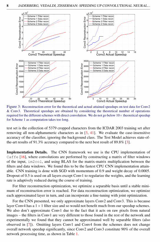
Figure 3: Reconstruction error for the theoretical and actual attained speedups on test data for Conv2& Conv3. Theoretical speedups are obtained by considering the theoretical number of operationsrequired for the different schemes with direct convolution. We do not go below 10⇥ theoretical speedupfor Scheme 1 as computation takes too long.

test set is the collection of 5379 cropped characters from the ICDAR 2003 training set afterremoving all non-alphanumeric characters as in [3, 41]. We evaluate the case-insensitiveaccuracy of the classifier, ignoring the background class. The Test Model achieves state-of-the-art results of 91.3% accuracy compared to the next best result of 89.8% [3].

Implementation Details. The CNN framework we use is the CPU implementation ofCaffe [16], where convolutions are performed by constructing a matrix of filter windowsof the input, im2col, and using BLAS for the matrix-matrix multiplication between thefilters and data windows. We found this to be the fastest CPU CNN implementation attain-able. CNN training is done with SGD with momentum of 0.9 and weight decay of 0.0005.Dropout of 0.5 is used on all layers except Conv1 to regularize the weights, and the learningrate is adaptively reduced during the course of training.

For filter reconstruction optimization, we optimize a separable basis until a stable mini-mum of reconstruction error is reached. For data reconstruction optimization, we optimizeeach approximated layer in turn, and can incorporate a fine-tuning with joint optimization.

For the CNN presented, we only approximate layers Conv2 and Conv3. This is becauselayer Conv4 has a 1⇥1 filter size and so would not benefit much from our speedup schemes.We also don’t approximate Conv1 due to the fact that it acts on raw pixels from naturalimages – the filters in Conv1 are very different to those found in the rest of the network andexperimentally we found that they cannot be approximated well by separable filters (alsoobserved in [7]). Omitting layers Conv1 and Conv4 from the schemes does not changeoverall network speedup significantly, since Conv2 and Conv3 constitute 90% of the overallnetwork processing time, as shown in Table 1.

JADERBERG, VEDALDI, ZISSERMAN: SPEEDING UP CONVOLUTIONAL NEURAL... 9

1 2 3 4 50

5

10

15

20

Full net speedup factor

Perc

ent l

oss

in a

ccur

acy

Scheme 1

Filter reconstructionData reconstructionJoint data reconstruction

1 2 3 4 5 6 70

5

10

15

20

Full net speedup factor

Perc

ent l

oss

in a

ccur

acy

Scheme 2

Filter reconstructionData reconstructionJoint data reconstruction

(a) (b) (c)

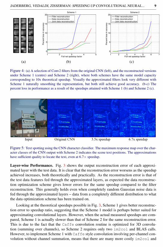
Figure 4: (a) A selection of Conv2 filters from the original CNN (left), and the reconstructed versionsunder Scheme 1 (centre) and Scheme 2 (right), where both schemes have the same model capacitycorresponding to 10x theoretical speedup. Visually the approximated filters look very different withScheme 1 naturally smoothing the representation, but both still achieve good accuracy. (b-c) Thepercent loss in performance as a result of the speedups attained with Scheme 1 (b) and Scheme 2 (c).

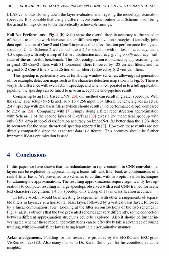
Figure 5: Text spotting using the CNN character classifier. The maximum response map over the char-acter classes of the CNN output with Scheme 2 indicates the scene text positions. The approximationshave sufficient quality to locate the text, even at 6.7⇥ speedup.

Layer-wise Performance. Fig. 3 shows the output reconstruction error of each approxi-mated layer with the test data. It is clear that the reconstruction error worsens as the speedupachieved increases, both theoretically and practically. As the reconstruction error is that ofthe test data features fed through the approximated layers, as expected the data reconstruc-tion optimization scheme gives lower errors for the same speedup compared to the filterreconstruction. This generally holds even when completely random Gaussian noise data isfed through the approximated layers – data from a completely different distribution to whatthe data optimization scheme has been trained on.

Looking at the theoretical speedups possible in Fig. 3, Scheme 1 gives better reconstruc-tion error to speedup ratio, suggesting that the Scheme 1 model is perhaps better suited forapproximating convolutional layers. However, when the actual measured speedups are com-pared, Scheme 1 is actually slower than that of Scheme 2 for the same reconstruction error.This is due to the fact that the Caffe convolution routine is optimized for 3D convolu-tion (summing over channels), so Scheme 2 requires only two im2col and BLAS calls.However, to implement Scheme 1 with Caffe style convolution involving per-channel con-volution without channel summation, means that there are many more costly im2col and

10 JADERBERG, VEDALDI, ZISSERMAN: SPEEDING UP CONVOLUTIONAL NEURAL...

BLAS calls, thus slowing down the layer evaluation and negating the model approximationspeedups. It is possible that using a different convolution routine with Scheme 1 will bringthe actual timings closer to the theoretically achievable timings.

Full Net Performance. Fig. 4 (b) & (c) show the overall drop in accuracy as the speedupof the end-to-end network increases under different optimization strategies. Generally, jointdata optimization of Conv2 and Conv3 improves final classification performance for a givenspeedup. Under Scheme 2 we can achieve a 2.5⇥ speedup with no loss in accuracy, and a4.5⇥ speedup with only a drop of 1% in classification accuracy, giving 90.3% accuracy – stillstate-of-the-art for this benchmark. The 4.5⇥ configuration is obtained by approximating theoriginal 128 Conv2 filters with 31 horizontal filters followed by 128 vertical filters, and theoriginal 512 Conv3 filters with 26 horizontal filters followed by 512 vertical filters.

This speedup is particularly useful for sliding window schemes, allowing fast generationof, for example, detection maps such as the character detection map shown in Fig. 5. There isvery little difference with even a 3.5⇥ speedup, and when incorporated in to a full applicationpipeline, the speedup can be tuned to give an acceptable end-pipeline result.

Comparing to an FFT based CNN [23], our method can result in greater speedups. Withthe same layer setup (5⇥5 kernel, 16⇥16⇥256 input, 384 filters), Scheme 2 gives an actual2.4⇥ speedup with 256 basis filters (which should result in no performance drop), comparedto 2.2⇥ in [23]. Comparing with [7], simply doing a filter reconstruction approximationwith Scheme 2 of the second layer of OverFeat [33] gives a 2⇥ theoretical speedup withonly 0.5% drop in top-5 classification accuracy on ImageNet, far better than the 1.2% dropin accuracy for the same theoretical speedup reported in [7]. However, these results are notdirectly comparable since the exact test data is different. This accuracy should be furtherimproved if data optimization is used.

4 Conclusions

In this paper we have shown that the redundancies in representation in CNN convolutionallayers can be exploited by approximating a learnt full rank filter bank as combinations of arank-1 filter basis. We presented two schemes to do this, with two optimization techniquesfor attaining the approximations. The resulting approximations require significantly less op-erations to compute, resulting in large speedups observed with a real CNN trained for scenetext character recognition: a 4.5⇥ speedup, only a drop of 1% in classification accuracy.

In future work it would be interesting to experiment with other arrangements of separa-ble filters in layers, e.g. a horizontal basis layer, followed by a vertical basis layer, followedby a linear combination layer. Looking at the filter reconstructions of the two schemes inFig. 4 (a), it is obvious that the two presented schemes act very differently, so the connectionbetween different approximation structures could be explored. Also it should be further in-vestigated whether these model approximations can be effectively taken advantage of duringtraining, with low-rank filter layers being learnt in a discriminative manner.

Acknowledgements. Funding for this research is provided by the EPSRC and ERC grantVisRec no. 228180. Also many thanks to Dr. Karen Simonyan for his countless, valuableinsights.

JADERBERG, VEDALDI, ZISSERMAN: SPEEDING UP CONVOLUTIONAL NEURAL... 11

References[1] http://algoval.essex.ac.uk/icdar/datasets.html.

[2] http://www.iapr-tc11.org/mediawiki/index.php/kaist_scene_text_database.

[3] O. Alsharif and J. Pineau. End-to-End Text Recognition with Hybrid HMM MaxoutModels. In International Conference on Learning Representations, 2014.

[4] A. Bissacco, M. Cummins, Y. Netzer, and H. Neven. PhotoOCR: Reading text inuncontrolled conditions. In International Conference of Computer Vision, 2013.

[5] T. de Campos, B. R. Babu, and M. Varma. Character recognition in natural images.2009.

[6] M. Denil, B. Shakibi, L. Dinh, and N. de Freitas. Predicting parameters in deep learn-ing. In Advances in Neural Information Processing Systems, pages 2148–2156, 2013.

[7] E. Denton, W. Zaremba, J. Bruna, Y. LeCun, and R. Fergus. Exploiting linear structurewithin convolutional networks for efficient evaluation. arXiv preprint arXiv:1404.0736,2014.

[8] C. Farabet, Y. LeCun, K. Kavukcuoglu, E. Culurciello, B. Martini, P. Akselrod, andS. Talay. Large-scale fpga-based convolutional networks. Machine Learning on VeryLarge Data Sets, 2011.

[9] C. Farabet, C. Couprie, L. Najman, and Y. LeCun. Scene parsing with multiscalefeature learning, purity trees, and optimal covers. arXiv preprint arXiv:1202.2160,2012.

[10] I. J. Goodfellow, Y. Bulatov, J. Ibarz, S. Arnoud, and V. Shet. Multi-digit numberrecognition from street view imagery using deep convolutional neural networks. InInternational Conference on Learning Representations, 2013.

[11] I. J. Goodfellow, D. Warde-Farley, M. Mirza, A. Courville, and Y. Bengio. Maxoutnetworks. arXiv preprint arXiv:1302.4389, 2013.

[12] G. E. Hinton, N. Srivastava, A. Krizhevsky, I. Sutskever, and R. R. Salakhutdinov.Improving neural networks by preventing co-adaptation of feature detectors. arXivpreprint arXiv:1207.0580, 2012.

[13] F. Iandola, M. Moskewicz, S. Karayev, R. Girshick, T. Darrell, and K. Keutzer.Densenet: Implementing efficient convnet descriptor pyramids. arXiv preprintarXiv:1404.1869, 2014.

[14] M. Jaderberg, K. Simonyan, A. Vedaldi, and A. Zisserman. Synthetic data and artificialneural networks for natural scene text recognition. arXiv preprint arXiv:1406.2227,2014.

[15] M. Jaderberg, A Vedaldi, and A. Zisserman. Deep features for text spotting. In Euro-pean Conference on Computer Vision, 2014.

[16] Y. Jia. Caffe: An open source convolutional architecture for fast feature embedding.http://caffe.berkeleyvision.org/, 2013.

12 JADERBERG, VEDALDI, ZISSERMAN: SPEEDING UP CONVOLUTIONAL NEURAL...

[17] D. Karatzas, F. Shafait, S. Uchida, M. Iwamura, S. R. Mestre, J. Mas, D. F. Mota,J. Almazan, L. P. de las Heras, et al. ICDAR 2013 robust reading competition. InDocument Analysis and Recognition (ICDAR), 2013 12th International Conference on,pages 1484–1493. IEEE, 2013.

[18] K. Kavukcuoglu, P. Sermanet, Y. Boureau, K. Gregor, M. Mathieu, and Y. LeCun.Learning convolutional feature hierarchies for visual recognition. In NIPS, volume 1,page 5, 2010.

[19] A. Krizhevsky, I. Sutskever, and G. E. Hinton. ImageNet classification with deep con-volutional neural networks. In NIPS, volume 1, page 4, 2012.

[20] H. Lee, R. Grosse, R. Ranganath, and A. Y. Ng. Convolutional deep belief networks forscalable unsupervised learning of hierarchical representations. In Proceedings of the26th Annual International Conference on Machine Learning, pages 609–616. ACM,2009.

[21] S. Lucas. ICDAR 2005 text locating competition results. In Document Analysis andRecognition, 2005. Proceedings. Eighth International Conference on, pages 80–84.IEEE, 2005.

[22] F. Mamalet and C. Garcia. Simplifying convnets for fast learning. In Artificial NeuralNetworks and Machine Learning–ICANN 2012, pages 58–65. Springer, 2012.

[23] M. Mathieu, M. Henaff, and Y. LeCun. Fast training of convolutional networks throughffts. CoRR, abs/1312.5851, 2013.

[24] L. Neumann and J. Matas. A method for text localization and recognition in real-worldimages. In Proc. Asian Conf. on Computer Vision, pages 770–783. Springer, 2010.

[25] L. Neumann and J. Matas. Text localization in real-world images using efficientlypruned exhaustive search. In Proc. ICDAR, pages 687–691. IEEE, 2011.

[26] L. Neumann and J. Matas. Real-time scene text localization and recognition. In Proc.CVPR, volume 3, pages 1187–1190. IEEE, 2012.

[27] L. Neumann and J. Matas. Scene text localization and recognition with oriented strokedetection. In 2013 IEEE International Conference on Computer Vision (ICCV 2013),pages 97–104, California, US, December 2013. IEEE. ISBN 978-1-4799-2839-2. doi:10.1109/ICCV.2013.19.

[28] M. Oquab, L. Bottou, I. Laptev, and J. Sivic. Learning and transferring mid-level imagerepresentations using convolutional neural networks. In Computer Vision and PatternRecognition (CVPR), 2014.

[29] I. Posner, P. Corke, and P. Newman. Using text-spotting to query the world. In Proc.of the IEEE/RSJ Int. Conf. on Intelligent Robots and Systems (IROS), 2010.

[30] T. Quack. Large scale mining and retrieval of visual data in a multimodal context. PhDthesis, ETH Zurich, 2009.

JADERBERG, VEDALDI, ZISSERMAN: SPEEDING UP CONVOLUTIONAL NEURAL... 13

[31] R. Rigamonti, M. A. Brown, and V. Lepetit. Are sparse representations really relevantfor image classification? In Computer Vision and Pattern Recognition (CVPR), 2011IEEE Conference on, pages 1545–1552. IEEE, 2011.

[32] R. Rigamonti, A. Sironi, V. Lepetit, and P. Fua. Learning separable filters. In ComputerVision and Pattern Recognition (CVPR), 2013 IEEE Conference on, pages 2754–2761.IEEE, 2013.

[33] P. Sermanet, D. Eigen, X. Zhang, M. Mathieu, R. Fergus, and Y. LeCun. Overfeat:Integrated recognition, localization and detection using convolutional networks. arXivpreprint arXiv:1312.6229, 2013.

[34] A. Shahab, F. Shafait, and A. Dengel. ICDAR 2011 robust reading competition chal-lenge 2: Reading text in scene images. In Proc. ICDAR, pages 1491–1496. IEEE,2011.

[35] H. O. Song, S. Zickler, T. Althoff, R. Girshick, M. Fritz, C. Geyer, P. Felzenszwalb,and T. Darrell. Sparselet models for efficient multiclass object detection. In ComputerVision–ECCV 2012, pages 802–815. Springer, 2012.

[36] H. O. Song, T. Darrell, and R. B. Girshick. Discriminatively activated sparselets. InProceedings of the 30th International Conference on Machine Learning (ICML-13),pages 196–204, 2013.

[37] Y. Taigman, M. Yang, M. Ranzato, and L. Wolf. Deep-Face: Closing the gap to human-level performance in face verification. In IEEE CVPR, 2014.

[38] A. Toshev and C. Szegedy. DeepPose: Human pose estimation via deep neural net-works. arXiv preprint arXiv:1312.4659, 2013.

[39] K. van de Sande, J. Uijlings, T. Gevers, and A. Smeulders. Segmentation as selectivesearch for object recognition. In Computer Vision (ICCV), 2011 IEEE InternationalConference on, pages 1879–1886. IEEE, 2011.

[40] V. Vanhoucke, A. Senior, and M. Z. Mao. Improving the speed of neural networks oncpus. In Proc. Deep Learning and Unsupervised Feature Learning NIPS Workshop,2011.

[41] K. Wang, B. Babenko, and S. Belongie. End-to-end scene text recognition. In Proc.ICCV, pages 1457–1464. IEEE, 2011.

[42] T. Wang, D. J. Wu, A. Coates, and A. Y. Ng. End-to-end text recognition with con-volutional neural networks. In Pattern Recognition (ICPR), 2012 21st InternationalConference on, pages 3304–3308. IEEE, 2012.

[43] H. Yang, B. Quehl, and H. Sack. A framework for improved video text detection andrecognition. In Int. Journal of Multimedia Tools and Applications (MTAP), 2012.