Speeding up Automatic Hyperparameter Optimization of Deep Neural Networksby Extrapolation of Learning Curves

Tobias Domhan, Jost Tobias Springenberg, Frank HutterUniversity of Freiburg

Freiburg, Germany{domhant,springj,fh}@cs.uni-freiburg.de

AbstractDeep neural networks (DNNs) show very strongperformance on many machine learning problems,but they are very sensitive to the setting of theirhyperparameters. Automated hyperparameter op-timization methods have recently been shown toyield settings competitive with those found by hu-man experts, but their widespread adoption is ham-pered by the fact that they require more compu-tational resources than human experts. Humanshave one advantage: when they evaluate a poorhyperparameter setting they can quickly detect (af-ter a few steps of stochastic gradient descent) thatthe resulting network performs poorly and termi-nate the corresponding evaluation to save time. Inthis paper, we mimic the early termination of badruns using a probabilistic model that extrapolatesthe performance from the first part of a learningcurve. Experiments with a broad range of neuralnetwork architectures on various prominent objectrecognition benchmarks show that our resulting ap-proach speeds up state-of-the-art hyperparameteroptimization methods for DNNs roughly twofold,enabling them to find DNN settings that yield betterperformance than those chosen by human experts.

1 IntroductionDeep neural networks (DNNs) trained via backpropaga-tion currently constitute the state-of-the-art for many clas-sification problems, such as object recognition from im-ages [Krizhevsky et al., 2012; Donahue et al., 2014] or speechrecognition from audio data (see [Deng et al., 2013] for a re-cent review). Unfortunately, they are also very sensitive tothe setting of their hyperparameters [Montavon et al., 2012].While good settings are hard to find by non-experts, au-tomatic hyperparameter optimization methods have recentlybeen shown to yield performance competitive with human ex-perts, and in some cases even surpassed them [Bergstra et al.,2011; Snoek et al., 2012; Dahl et al., 2013; Bergstra et al.,2013].

However, fitting large DNNs is computationally expensiveand the time overhead of automated hyperparameter opti-mization hampers its widespread adoption. Instead, many hu-

man deep learning experts still perform manual hyperparam-eter search, relying on a “bag of tricks” to determine modelhyperparameters and learning rates for stochastic gradient de-scent (SGD) [Montavon et al., 2012]. Using this acquiredknowledge they can often tell after a few SGD steps whetherthe training procedure will converge to a model with compet-itive performance or not. To save time, they then prematurelyterminate runs expected to perform poorly, allowing them tomake more rapid progress than automated methods (whichtrain even poor models until the end).

In this work, we mimic this early termination of bad runswith the help of a probabilistic model that extrapolates perfor-mance from the first part of a learning curve to its remainder,enabling us to automatically identify and terminate bad runsto save time. After discussing related work on hyperparame-ter optimization and studies of learning curves (Section 2), weintroduce our probabilistic approach for extrapolating learn-ing curves and show how to use it to devise a predictive ter-mination criterion that can be readily combined with any hy-perparameter optimization method (Section 3). Experimentswith different neural network architectures on the prominentobject recognition benchmarks CIFAR-10, CIFAR-100 andMNIST show that predictive termination speeds up currenthyperparameter optimization methods for DNNs by roughlya factor of two, enabling them to find DNN settings that yieldbetter performance than those chosen by human experts (Sec-tion 4).

2 Foundations and Related WorkWe first review modern hyperparameter optimization meth-ods and previous attempts to model learning curves.

2.1 Hyperparameter Optimization MethodsGiven a machine learning algorithm A having hyperparame-ters λ1, . . . , λn with respective domains Λ1, . . . ,Λn, we de-fine its hyperparameter space as Λ = Λ1 × · · · × Λn. Foreach hyperparameter setting λ ∈ Λ, we use Aλ to denotethe learning algorithm A using this setting. We further usel(λ) = L(Aλ,Dtrain,Dvalid) to denote the validation loss(e.g., misclassification rate) that Aλ achieves on data Dvalidwhen trained on Dtrain. The hyperparameter optimizationproblem is then to find λ ∈ Λ minimizing l(λ).

For decades, the de-facto standard for hyperparameter op-timization in machine learning has been a simple grid search.

Other approaches proposed over the years include racing al-gorithms [Maron and Moore, 1994] and gradient search [Ben-gio, 2000]. Recently, it has been shown that a simple ran-dom search can perform much better than grid search, par-ticularly for high-dimensional problems with low intrinsicdimensionality [Bergstra and Bengio, 2012]. More sophis-ticated Bayesian optimization methods perform even bet-ter and have yielded new state-of-the-art results for sev-eral datasets [Bergstra et al., 2011; Hutter et al., 2011;Snoek et al., 2012; Bergstra et al., 2013].

Bayesian Optimization (see, e.g., [Jones et al., 1998;Brochu et al., 2010]) constructs a probabilistic modelM off based on point evaluations of f and any available prior in-formation, uses modelM to select subsequent configurationsλ to evaluate, updatesM based on the new measured perfor-mance at λ, and iterates.

The three most popular implementations of Bayesian op-timization are Spearmint [Snoek et al., 2012], which usesa Gaussian process (GP) [Rasmussen and Williams, 2006]model for M; SMAC [Hutter et al., 2011], which uses ran-dom forests [Breiman, 2001] modified to yield an uncer-tainty estimate [Hutter et al., 2014]; and the Tree ParzenEstimator (TPE) [Bergstra et al., 2011], which constructs adensity estimate over good and bad instantiations of eachhyperparameter to build M. Eggensperger et al. [2013]empirically compared these three systems, concluding thatSpearmint’s GP-based approach performs best for problemswith few numerical (and no other) hyperparameters, and thatSMAC’s and TPE’s tree-based approach performs best forhigh-dimensional and partly discrete hyperparameter opti-mization problems, as they occur in optimizing DNNs. Wetherefore use SMAC and TPE in this study.

2.2 Modeling Learning CurvesThe term learning curve appears in the literature for describ-ing two different phenomena: (1) the performance of an iter-ative machine learning algorithm as a function of its trainingtime or number of iterations; and (2) the performance of amachine learning algorithm as a function of the size of thedataset it has available for training. While our work concernslearning curves of type 1, we describe related work on mod-elling both types of learning curves.

Learning curves of type 1 are very popular for visualizingthe concept of overfitting: while performance on the trainingset tends to improve over time, test performance often de-grades eventually. The study of these learning curves has ledto early stopping heuristics aiming to terminate training be-fore overfitting occurs (see, e.g., [Yao et al., 2007]). We notethat the goal behind our new predictive termination criterionis different: we predict validation performance and terminatea run when it is unlikely to beat the performance of the bestmodel we have encountered so far.

In parallel to our work, Swersky et al. [2014] devised a GP-based Bayesian optimization method that includes a learningcurve model. They used this model for temporarily paus-ing the training of machine learning models, in order to ex-plore several promising hyperparameter configurations for ashort time and resume training on the most promising mod-els later on. Swersky et al. [2014] successfully applied this

technique to matrix factorization, online Latent Dirichlet Al-location (LDA) and logistic regression. However, so far itdoes not work well for deep neural networks, possibly sinceit is limited to one particular parametric learning curve modelthat may not describe learning curves of deep networks well.1

Learning curves of type 2 have been studied to extrapolateperformance from smaller to larger datasets. In early work,Frey and Fisher [1999] estimated the amount of data neededby a decision tree to achieve a desired accuracy using lin-ear, logarithmic, exponential and power law parametric mod-els. Subsequent work predicted the performance of multi-ple machine learning algorithms using a total of 6 parametricmodels: a power law model with two and three parameters,a logarithmic model, the vapor pressure model, the Morgan-Mercer-Flodin (MMF) model, and the Weibull model [Gu etal., 2001]. More recently, e.g., Kolachina et al. [2012] pre-dicted how a statistical machine translation system would per-form if more data was available; they used 6 parametric mod-els and concluded that the three parameter power law is mostsuitable for their task.

All these approaches for extrapolating learning curves havein common that they use maximum likelihood fits of eachparametric model by itself. In contrast to the probabilistic ap-proach we propose in this work, the curve models are thusneither combined to increase their representative power nordo they account for uncertainty in the data and model param-eters.

3 Extrapolation of Learning CurvesIn this paper, we focus on learning curves that describe theperformance of DNNs as a function of the number of stochas-tic gradient descent (SGD) steps. We measure performance asclassification accuracy on a validation set.

3.1 Learning Curve ModelIn this section, we describe how we probabilistically extra-polate from a short initial portion of a learning curve to alater point. When running SGD on DNNs we measure vali-dation performance in regular intervals. Let y1:n denote theobserved performance values for the first n intervals. In ourproblem setup, we observe y1:n and aim to predict perfor-mance ym after a large number of intervalsm� n. We solvethis problem using a probabilistic model.

Parametric Learning Curve ModelsOur basic approach is to model the partially observedlearning curve y1:n by a set of parametric model families{f1, . . . , fK}. Each of these parametric functions fk is de-scribed through a set of parameters θk. Assuming additiveGaussian noise ε ∼ N (0, σ2), we can use each fk to modelperformance at time step t as yt = fk(t|θ)+ε; the probabilityof a single observation yt under model fk is hence given as

p(yt|θk, σ2) = N (yt; fk(t|θk), σ2). (1)

We chose a large set of parametric curve models from theliterature whose shape coincides with our prior knowledge

1Based on personal communication with the authors.

Reference name Formulavapor pressure exp(a+ b

x+ c log(x))

pow3 c− ax−α

log log linear log(a log(x) + b)

Hill3 ymaxxη

κη+xη

log power a

1+(xeb

)cpow4 c− (ax+ b)−α

MMF α− α−β1+(κx)δ

exp4 c− e−axα+b

Janoschek α− (α− β)e−κxδ

Weibull α− (α− β)e−(κx)δ

ilog2 c− alog x

Figure 1: Left: A typical learning curve and extrapolations from its first part (the end of which is marked with a vertical line),with each of the 11 individual parametric models. The legend is sorted by the residual of the predictions at epoch 300. Right:the formulas for our 11 parameteric learning curve models fk(x).

about the form of learning curves: They are typically in-creasing, saturating functions; for example functions from thepower law or the sigmoidal family. In total we consideredK = 11 different model families; Figure 1 shows an examplefor how each of these functions would model a typical learn-ing curve and also provides their parametric formulas. Wenote that all of these models capture certain aspects of learn-ing curves, but that no single model can describe all learningcurves by itself, motivating us to combine the models in aprobabilistic framework.

A Weighted Probabilistic Learning Curve ModelInstead of selecting an individual model we combine all Kmodels into a single, more powerful, model. This combinedmodel is given by a weighted linear combination:

fcomb(t|ξ) =

K∑k=1

wkfk(t|θk), (2)

where the new combined parameter vector

ξ = (w1, . . . , wK ,θ1, . . . ,θK , σ2) (3)

comprises a weight wk for each model, the individualmodel parameters θk, and the noise variance σ2, and yt =fcomb(t|ξ) + ε.

Given this model, a simple approach would be to find amaximum likelihood estimate for all parameters. However,this would not properly model the uncertainty in the modelparameters. Since our predictive termination criterion aimsat only terminating runs that are highly unlikely to improveon the best run observed so far we need to model uncertaintyas truthfully as possible and will hence adopt a Bayesian per-spective, predicting values ym using Markov Chain MonteCarlo (MCMC) inference.

To enable such probabilistic inference we also need toplace a prior probability on all parameters. It would be sim-plest to choose an uninformative prior, such that

p(ξ) ∝ 1. (4)

However, with such an uninformative prior we put posi-tive probability mass on parameterizations that yield learningcurves which decrease after some time. To avoid this situa-tion, we explicitly encode our knowledge into the prior thatwell-behaved learning curves are increasing saturating func-tions. We also restrict the weights to be positive only, allow-ing us to interpret each individual model as a non-negativeadditive component of a learning curve. This has the niceside effect that the predicted curve will only be flat once allmodels have flattened out.

Concretely, we define a new prior distribution over ξ,which encodes the above intuition, as

p(ξ)∝

(K∏

k=1

p(wk)p(θk)

)p(σ2)1(fcomb(1|ξ)<fcomb(m|ξ))

(5)and for all k

p(wk) ∝{

1 if wk > 0

0 otherwise. (6)

The p(θk) and p(σ2) are still set to be uninformative, butare mentioned for the sake of completeness. The indicatorfunction 1(fcomb(1|ξ) < fcomb(m|ξ)) ensures that no patho-logical model that decreases from the initial value to the pointof prediction m gets any probability mass. Finally, the prioron the weights p(wk) ensures weights are never negative. Fig-ure 2 visualizes the problem this modified prior solves: whilethe uninformative prior yields learning curves that decreaseover time (Figure 2a), our new prior yields increasing satu-rating curves (Figure 2b).

With these definitions in place we can finally performMCMC sampling over the joint parameter and weight spaceξ by drawing S samples ξ1, . . . , ξS from the posterior

P (ξ|y1:n) ∝ P (y1:n|ξ)P (ξ), (7)

where P (y1:n|ξ) for the model combination is given asP (y1:n|ξ) = Πn

t=1N (yt; fcomb(t|ξ), σ2). To initialize thesampling procedure, we set all model parameters θk to

(a) Uninformative prior (b) Prior enforcing positive weights and increasing functions

Figure 2: The effect of the prior. We show posterior predictions using the uninformative prior and the prior encoding ourknowledge about learning curves. The vertical line marks the point of prediction.

their (per-model) maximum likelihood estimate. The modelweights are initialized uniformly, that is wk = 1

K . The noiseparameter is also initialized to its maximum likelihood esti-

mate σ2 = 1n

n∑t=1

(yt − fcomb(t|ξ))2.

A sample approximation for ym with m > n can then beformed as

E[ym|y1:n] ≈ 1

S

S∑s=1

fcomb(m|ξs). (8)

More importantly, since we also have an estimate ofthe parameter uncertainty and the predictive distributionP (ym|y1:n, ξ) is a Gaussian for each fixed ξ, we can estimatethe probability that ym exceeds a certain value y as

P (ym ≥ y|y1:n) =

∫P (ξ|y1:n)P (ym > y|ξ)dξ (9)

≈ 1

S

S∑s=1

P (ym > y|ξs) (10)

=1

S

S∑s=1

(1− Φ(y; fcomb(m|ξs), σ2

s)), (11)

where Φ(·;µ, σ2) is the cumulative distribution function ofthe Gaussian with mean µ and variance σ2.

We note that the entire learning curve extrapolation processis robust and fully automated, with MCMC sampling takingcare of all free parameters.

3.2 Speeding up Hyperparameter OptimizationWe use our predictive models to speed up hyperparameteroptimizers as follows. Firstly, while the hyperparameter op-timizer is running we keep track of the best performance yfound so far (we initialize y to −∞). Each time the opti-mizer queries the performance l(λ) of a hyperparameter set-ting λ we train a DNN using λ as usual, except that we ter-minate this run early if our extrapolation model predicts thenetwork to eventually yield worse performance than y. Moreprecisely, at regular intervals i during SGD training we mea-sure and save validation set performance yi. There are emax

epochs, k such intervals per epoch, and every p epochs, wegather the performance values y1:n of the n intervals so farand run MCMC to probabilistically extrapolate performanceto the final stepm = k×emax. We then consider the predictedprobability P (ym ≥ y|y1:n) that the network, after trainingfor m intervals, will exceed the performance y. If this prob-ability is above a threshold δ then training continues as usualfor the next p epochs. Otherwise, training is terminated andwe return the expected validation error 1−E[ym|y1:n] (whereE[ym|y1:n] is the expected accuracy from Equation 8) to thehyperparameter optimizer in lieu of the real (yet unknown)loss. We dub this procedure the predictive termination crite-rion. It is agnostic to the precise hyperparameter optimizerused and we will evaluate its performance using two differentstate-of-the-art optimizers.

We also note that, importantly, the network training doesnot need to be paused while the termination criterion is run:we simply run MCMC sampling on the available CPU coreswhile the network training continues on the GPU.

4 ExperimentsTo test our predictive termination criterion under a wide va-riety of different conditions, we performed experiments ona broad range of DNN architectures and datasets, carryingout a combined search over architectures and hyperparam-eters using two state-of-the-art hyperparameter optimizationmethods.

4.1 Experimental SetupWe used three popular datasets concerning object recogni-tion from small-sized images: the image recognition datasetsCIFAR-10 and CIFAR-100 [Krizhevsky, 2009] and the wellknown MNIST dataset [LeCun et al., 1989]. CIFAR-10and CIFAR-100 each contain 50,000 training and 10,000 testRGB images with 32× 32 pixels that were taken from a sub-set of the 80-million tiny images database. While CIFAR-10contains images from 10 categories, CIFAR-100 contains im-ages from 100 categories and thus contains 10 times fewerexamples per class. The MNIST dataset is a classic objectrecognition dataset consisting of 60,000 training and 10,000

test images with 28× 28 pixels depicting hand-written digitsto be classified into 10 digit classes.

For performing the hyperparameter search on CIFAR-10and CIFAR-100, we randomly split the training data intotraining and validation sets containing 40,000 and 10,000 ex-amples, respectively. Likewise, for MNIST, we split the train-ing data into a training set containing 50,000 examples and avalidation set containing 10,000 examples. We used the deeplearning framework CAFFE [Jia et al., 2014] to train DNNson a single GPU per run. We further used the hyperparameteroptimization toolbox HPOLIB [Eggensperger et al., 2013] incombination with our implementation of the predictive termi-nation criterion based on learning curve prediction, using theMCMC sampler EMCEE [Foreman-Mackey et al., 2013].

For the predictive termination criterion we set the thresholdto δ = 0.05 in all experiments, that is, we stopped training anetwork if our extrapolation model was 95% certain that itwould not improve over the best known performance y whenfully trained. We ran the predictive termination criterion ev-ery p = 30 epochs. The number of intervals k per SGD epochat which we evaluate validation performance was chosen sep-arately for each architecture to reflect the cost of computingpredictions on the validation data; we used k = 10 for fullyconnected networks and k = 2 for convolutional networks.

4.2 Fully Connected NetworksIn the first experiment, we trained fully connected networksfor classification on a preprocessed variant of CIFAR-10 andon MNIST. To make training a fully connected network onCIFAR-10 feasible we used the same pipeline as Swerskyet al. [2013], who followed the approach from Coates etal. [2011] to create preprocessed CIFAR-10 features that actas a fixed convolutional layer while keeping the requiredcomputation time manageable. The pipeline first runs unsu-pervised k-means (with 400 centroids) on small patches of6 × 6 pixels that are randomly extracted from the CIFAR-10training set. It then builds a feature vector by convolving eachimage in CIFAR-10 with the centroids and averaging the re-sponses over parts of the image. After this preprocessing step,the network contains only fully connected layers to classifythe preprocessed data. We evaluated the benefits that our pre-dictive termination criterion yields in combination with threedifferent hyperparameter optimizers: SMAC, TPE, and ran-dom search (all described in Section 2.1). Each hyperparam-eter optimizer had a budget of evaluating a total of 100 net-works. The maximum number of epochs emax was 285.

In the MNIST experiment we fed the raw 784 pixel valuesto the fully connected networks. Our setup is thus comparableto most results on fully connected networks from the litera-ture, e.g., the recent results on training dropout networks toclassify MNIST [Srivastava et al., 2014]. Training a singlenetwork on MNIST required between 5 and 20 minutes, andthe hyperparameter optimizers had a fixed budget of evaluat-ing a total of 500 networks.

DNN HyperparametersThe hyperparameters for the fully connected network controlseveral architectural choices and hyperparameters related tothe optimization procedure. They include global hyperpa-

Network hyperparametersHyperparameter min max defaultinit. learning rate (log) 1× 10−7 0.5 0.001learning rate schedule (choice) {inv, fixed} fixedinv schedule2: lr. half-life (cond) 1 50 25inv schedule2: p (cond) 0.5 1. 0.71momentum 0 0.99 0.6weight decay (log) 5× 10−7 0.05 0.0005batch size B 10 1000 100number of layers 1 6 1input dropout (Boolean) {true, false} falseinput dropout rate (cond) 0.05 0.8 0.4

Fully connected layer hyperparametersHyperparameter min max defaultnumber of units 128 6144 1024weight filler type (choice) {Gaussian, Xavier} GaussianGaussian weight init σ (log; cond) 1× 10−6 0.1 0.005bias init (choice) {const-zero, const-value} const-zeroconstant value bias filler (cond) 0 1 0.5dropout enabled (Boolean) {true, false} truedropout ratio (cond) 0.05 0.95 0.5

Table 1: Hyperparameters for the fully connected networksand their ranges; lr. stands for learning rate, log indicates thatthe hyperparameter is optimized on a log scale, and cond in-dicates that the hyperparameter is conditional on being acti-vated by the Boolean hyperparameter above it.

rameters (which apply to the whole network) and per-layerhyperparameters; since the number of layers is a hyperpa-rameter itself, all hyperparameters of layer i are conditionalon the number of layers being at least i. Both our hyperpa-rameter optimizers SMAC and TPE can natively handle suchconditional hyperparameters to solve the combined architec-ture search and hyperparameter optimization problem. Weused stochastic gradient descent with momentum in all ex-periments. The learning rate was either fixed or changed ac-cording to the inv schedule2. All units in the network use rec-tified linear activation functions, and a softmax layer with di-mensionality 10 is placed at the end to predict the 10 classes.Weights are either initialized with Gaussian noise or with themethod proposed by Glorot and Bengio [2010]. Biases onthe other hand are either initialized to zero or to a constantvalue. Dropout is optionally also applied to the input of thenetwork. Table 1 details all hyperparameters, along with theirranges and the default values used to start the search; in to-tal, the hyperparameter space to be searched has 10(networkhyperparams) + 6(layers) × 7(hyperparams per layer) = 52hyperparameters.

Results for preprocessed CIFAR-10Figures 3a and 3b illustrate the speedups that our predic-tive termination yielded for training fully connected networkson preprocessed CIFAR-10 with SMAC and TPE. We raneach hyperparameter optimizer 5 times with different random

2The inv schedule is defined as αt = α0(1+γt)−p, where α0 is

the initial learning rate. In order to be able to set bounds intuitively,instead of parameterizing γ directly we make the half-life of α a newhyperparameter, which for a given p can be transformed back into γ.

(a) SMAC on k-means CIFAR-10 (b) TPE on k-means CIFAR-10 (c) SMAC on MNIST

Figure 3: Benefit of predictive termination for SMAC and TPE when optimizing hyperparameters of fully connected networks.(a-b) Results for the preprocessed CIFAR-10 dataset (a) and (b). (c) Same plot for SMAC MNIST.

Method # centroids Error (%)SVM [Coates et al., 2011] 4000 20.40%SVM [Coates et al., 2011] 1600 22.10%DNN [Swersky et al., 2013] 400 21.10%DNN (SMAC) 400 19.22%DNN (TPE) 400 20.18%DNN (random search) 400 19.90%

Table 2: Comparison of classification results on the k-meansfeatures extracted from the CIFAR10 dataset for different op-timizers in comparison to previously published results.

seeds and show means and standard deviations of their vali-dation errors across these runs. While all optimizers achievedstrong performance for this architecture (around 20% valida-tion error), their computational time requirements to achievethis level of performance differed greatly. As Figure 3a andFigure 3b show, our predictive termination criterion sped upboth SMAC and TPE by at least a factor of two for reach-ing the same validation error as without it. Overall, the av-erage time needed per hyperparamter optimization run wasreduced from 40 to 18 hours. After this experiment, we ap-plied the best models found by each optimizer to the test datato compute the classification error. These results—togetherwith a comparison to random search and previous attemptsfor using k-means preprocessed CIFAR-10—are given in Ta-ble 2, showing that all optimizers we used found configu-rations with slightly better performance than the previouslypublished results for this architecture, with SMAC yieldingthe overall best result for this experiment.

Figure 4 shows the effect of our predictive termination cri-terion on the different DNN training runs: the predictive ter-mination criterion successfully terminated runs that do notreach top performance but rather converge slowly to mediocreresults. The figure also shows that it was possible to terminatemany poor runs quite early.

Results for MNISTFigure 3c illustrates the speedups that predictive terminationyielded for training fully connected networks on MNIST withSMAC. We only ran SMAC (10 runs) for this experimentsince it had yielded the best results for CIFAR-10 (cf. Ta-ble 2). Consistent with the results on CIFAR-10, SMACfound networks with good performance with and without pre-

Network hyperparametersHyperparameter min max defaultinit. learning rate (log) 1× 10−7 0.5 0.001momentum 0 0.99 0.6weight decay (log) 5× 10−7 0.05 0.0005number of pooling layers 2 3 2learning rate decay γ 0.9 1. 0.9998

Convolutional layer hyperparametersHyperparameter min max defaultGaussian weight init σ (log) 1× 10−6 0.1 0.005weight lr. multiplier (log) 0.1 10.0 1.number of units (small/large CNN) 16/64 64/192 32/96

Table 3: Hyperparameters for the CNNs together with theirranges; lr. stands for learning rate, log indicates that the hy-perparameter is optimized on a log scale.

dictive termination (reaching approximately 1% validation er-ror) and was much faster when using the predictive termina-tion criterion: it reached 1% validation error in about 60%of the time it took a standard SMAC run to achieve the sameperformance.

4.3 Small Convolutional Neural NetworksTo study the generality of our learning curve extrapolationmodels, next, we turned to the problem of optimizing convo-lutional neural networks (CNNs), which constitute the state-of-the-art for visual object recognition (see [Krizhevsky etal., 2012; Jarrett et al., 2009] for recent explanations of con-volutional layers). For this experiment we used the CIFAR-10 and CIFAR-100 datasets. The images from both datasetswere preprocessed using a whitening transform, following thepractice outlined by Goodfellow et al. [2013]. Other than thatthe CNNs were trained on the raw pixel images.

Small CNN HyperparametersAt the core, our CNNs no longer contain fully connected lay-ers but rather use convolutional layers only, followed by asoftmax classification layer. These layers extract features byconvolving the input image or—for deeper layers—the outputof the previous layer with a set of filters. Convolutional lay-ers are regularly followed by dimensionality reduction steps(or pooling steps) which reduce the spatial dimensionality of

(a) Without predictive termination (b) Random subset of Figure 4a (c) With predictive termination

Figure 4: Comparison of learning curves for fully connected networks on CIFAR-10 with and without our predictive terminationcriterion. Best viewed in color. The plots contain all learning curves from the 10 runs of SMAC and TPE.

the feature map. In our first experiment with small CNNs, wemodel the hyperparameter space after the prominent archi-tecture from Krizhevsky et al. [2012]. Concretely, we builda hyperparameter space that mimics the layers-18pct configfrom cuda-convnet3. Table 3 summarizes this hyperparame-ter space. In contrast to the experiments with fully connectednetworks, we now parameterized the number of layers indi-rectly, by choosing the number of pooling layers (2 − 3). Aconvolutional layer is then always placed between these pool-ing layers. Each pooling layer always halves the input sizeby using max-pooling. The convolutional kernel size in eachlayer of our small CNNs is set to 5 × 5. These restrictionsalso make training quite fast (approximately 30 minutes pernetwork). Overall, our small CNNs contain 5 network hyper-parameters and 3 layer hyperparameters (conditioned on thenumber of convolutional layers used), resulting in a total of5 + 3× 3 = 14 configurable hyperparameters.

Results for Small CNNs on CIFAR-10We optimized the small CNN hyperparameter space using 10runs of both SMAC and TPE, with and without predictivetermination. Each run had a maximum budget of evaluating150 configurations. The maximum number of epochs emaxwas 100. While all optimizers eventually found configura-tions with good validation performance of around 20% error,SMAC gave slightly better results on average (19.4%± 0.2%error vs. 20%± 0.4% for TPE). We thus only present the re-sults for SMAC here due to space constraints.

Figure 5a shows that predictive termination again sped upSMAC by a factor of at least two for finding the same vali-dation error as without it. As shown in Figure 5b, predictivetermination again consistently stopped bad runs early. Whenthe best resulting configuration in terms of validation errorwas re-trained on the complete CIFAR-10 training dataset, itachieved a test error of 17.2% – slightly better than the base-line model (layers-18pct with 18% test error). A completecomparison of the test error for the best configuration foundby the different optimizers is given in Table 4 (top).

3http://code.google.com/p/cuda-convnet/

CIFAR-10 classification errorMethod Error (%)Small CNN + TPE 18.12%Small CNN + SMAC 17.47%Small CNN + TPE with pred. termination 18.08%Small CNN + SMAC with pred. termination 17.20%

CIFAR-100 classification errorMethod Error (%)Small CNN + SMAC 42.21%Small CNN + SMAC with pred. termination 41.90%

Table 4: Test error on CIFAR-10 and CIFAR-100 for thebest hyperparameter configuration found for the small CNNsearch space.

Results for Small CNNs on CIFAR-100

For CIFAR-100, we again optimized the same small CNNhyperparameter space as for CIFAR-10. For this experiment,we only used SMAC (10 runs with and without predictivetermination) since it gave the best results in our experimentson CIFAR-10. As for CIFAR-10, each hyperparameter opti-mization run had a budget of evaluating 150 configurations.Figure 5c gives the results of this experiment. SMAC foundconfigurations with approximately 43% validation error bothwith and without the predictive termination criterion, but wassubstantially faster with predictive termination and reachedthe same quality almost two times faster. Using the best con-figuration found with and without predictive termination tore-train on the full CIFAR-100 training data yielded slightlybetter test set performance for predictive termination (41.90%vs. 42.21%); in comparison, adapting the layers-18pct toCIFAR-100 yields 45% test error.

4.4 Large Convolutional Networks

Finally, to test our learning curve prediction on state-of-the-art CNN models, we optimized the hyperparameters of a fam-ily of large convolutional networks on CIFAR-10.

(a) Small CNNs CIFAR-10(b) CNN learning curves with predictive ter-mination (CIFAR-10) (c) Small CNNs CIFAR-100

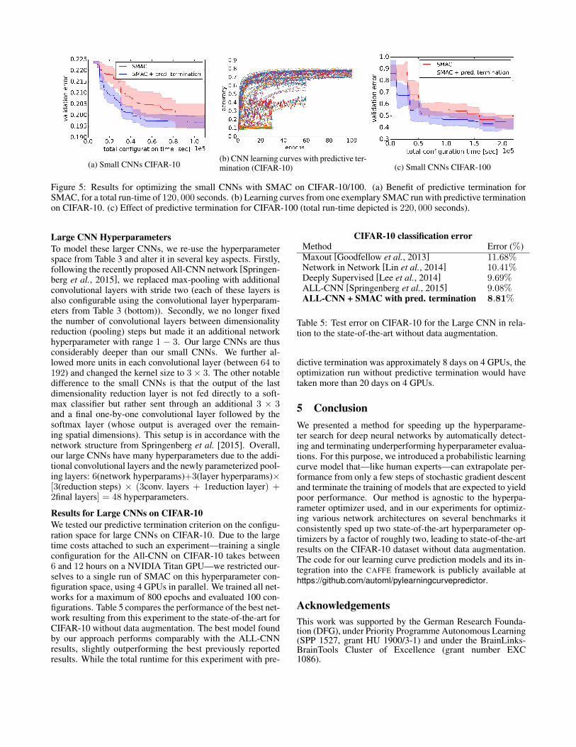
Figure 5: Results for optimizing the small CNNs with SMAC on CIFAR-10/100. (a) Benefit of predictive termination forSMAC, for a total run-time of 120, 000 seconds. (b) Learning curves from one exemplary SMAC run with predictive terminationon CIFAR-10. (c) Effect of predictive termination for CIFAR-100 (total run-time depicted is 220, 000 seconds).

Large CNN HyperparametersTo model these larger CNNs, we re-use the hyperparameterspace from Table 3 and alter it in several key aspects. Firstly,following the recently proposed All-CNN network [Springen-berg et al., 2015], we replaced max-pooling with additionalconvolutional layers with stride two (each of these layers isalso configurable using the convolutional layer hyperparam-eters from Table 3 (bottom)). Secondly, we no longer fixedthe number of convolutional layers between dimensionalityreduction (pooling) steps but made it an additional networkhyperparameter with range 1 − 3. Our large CNNs are thusconsiderably deeper than our small CNNs. We further al-lowed more units in each convolutional layer (between 64 to192) and changed the kernel size to 3× 3. The other notabledifference to the small CNNs is that the output of the lastdimensionality reduction layer is not fed directly to a soft-max classifier but rather sent through an additional 3 × 3and a final one-by-one convolutional layer followed by thesoftmax layer (whose output is averaged over the remain-ing spatial dimensions). This setup is in accordance with thenetwork structure from Springenberg et al. [2015]. Overall,our large CNNs have many hyperparameters due to the addi-tional convolutional layers and the newly parameterized pool-ing layers: 6(network hyperparams)+3(layer hyperparams)×[3(reduction steps) × (3conv. layers + 1reduction layer) +2final layers] = 48 hyperparameters.

Results for Large CNNs on CIFAR-10We tested our predictive termination criterion on the configu-ration space for large CNNs on CIFAR-10. Due to the largetime costs attached to such an experiment—training a singleconfiguration for the All-CNN on CIFAR-10 takes between6 and 12 hours on a NVIDIA Titan GPU—we restricted our-selves to a single run of SMAC on this hyperparameter con-figuration space, using 4 GPUs in parallel. We trained all net-works for a maximum of 800 epochs and evaluated 100 con-figurations. Table 5 compares the performance of the best net-work resulting from this experiment to the state-of-the-art forCIFAR-10 without data augmentation. The best model foundby our approach performs comparably with the ALL-CNNresults, slightly outperforming the best previously reportedresults. While the total runtime for this experiment with pre-

CIFAR-10 classification errorMethod Error (%)Maxout [Goodfellow et al., 2013] 11.68%Network in Network [Lin et al., 2014] 10.41%Deeply Supervised [Lee et al., 2014] 9.69%ALL-CNN [Springenberg et al., 2015] 9.08%ALL-CNN + SMAC with pred. termination 8.81%

Table 5: Test error on CIFAR-10 for the Large CNN in rela-tion to the state-of-the-art without data augmentation.

dictive termination was approximately 8 days on 4 GPUs, theoptimization run without predictive termination would havetaken more than 20 days on 4 GPUs.

5 ConclusionWe presented a method for speeding up the hyperparame-ter search for deep neural networks by automatically detect-ing and terminating underperforming hyperparameter evalua-tions. For this purpose, we introduced a probabilistic learningcurve model that—like human experts—can extrapolate per-formance from only a few steps of stochastic gradient descentand terminate the training of models that are expected to yieldpoor performance. Our method is agnostic to the hyperpa-rameter optimizer used, and in our experiments for optimiz-ing various network architectures on several benchmarks itconsistently sped up two state-of-the-art hyperparameter op-timizers by a factor of roughly two, leading to state-of-the-artresults on the CIFAR-10 dataset without data augmentation.The code for our learning curve prediction models and its in-tegration into the CAFFE framework is publicly available athttps://github.com/automl/pylearningcurvepredictor.

AcknowledgementsThis work was supported by the German Research Founda-tion (DFG), under Priority Programme Autonomous Learning(SPP 1527, grant HU 1900/3-1) and under the BrainLinks-BrainTools Cluster of Excellence (grant number EXC1086).

References[Bengio, 2000] Y. Bengio. Gradient-based optimization of hyper-

parameters. Neural Computation, 12(8):1889–1900, 2000.

[Bergstra and Bengio, 2012] J. Bergstra and Y. Bengio. Randomsearch for hyper-parameter optimization. JMLR, 13(1):281–305,2012.

[Bergstra et al., 2011] J. Bergstra, R. Bardenet, Y. Bengio, andB. Kégl. Algorithms for hyper-parameter optimization. InProc. of NIPS, pages 2546–2554, 2011.

[Bergstra et al., 2013] J. Bergstra, D. Yamins, and D.D. Cox. Mak-ing a science of model search: Hyperparameter optimization inhundreds of dimensions for vision architectures. In Proc. ofICML, pages 115–123, 2013.

[Breiman, 2001] L. Breiman. Random forests. Machine learning,45(1):5–32, 2001.

[Brochu et al., 2010] E. Brochu, V. M. Cora, and N. de Freitas. Atutorial on Bayesian optimization of expensive cost functions,with application to active user modeling and hierarchical rein-forcement learning. CoRR, abs/1012.2599, 2010.

[Coates et al., 2011] A. Coates, A. Y. Ng, and H. Lee. An analy-sis of single-layer networks in unsupervised feature learning. InProc. of AISTATS, pages 215–223, 2011.

[Dahl et al., 2013] G. Dahl, T. Sainath, and G. Hinton. Improv-ing deep neural networks for lvcsr using rectified linear units anddropout. In Proc. of ICASSP, pages 8609–8613. IEEE, 2013.

[Deng et al., 2013] L. Deng, G. Hinton, and B. Kingsbury. Newtypes of deep neural network learning for speech recognition andrelated applications: An overview. In Proc. of ICASSP, 2013.

[Donahue et al., 2014] J. Donahue, Y. Jia, O. Vinyals, J. Hoffman,N. Zhang, E. Tzeng, and T. Darrell. Decaf: A deep convolu-tional activation feature for generic visual recognition. In Proc. ofICML, 2014.

[Eggensperger et al., 2013] K. Eggensperger, M. Feurer, F. Hutter,J. Bergstra, J. Snoek, H. Hoos, and K. Leyton-Brown. Towardsan empirical foundation for assessing Bayesian optimization ofhyperparameters. In NIPS Workshop on Bayesian Optimizationin Theory and Practice (BayesOpt’13), 2013.

[Foreman-Mackey et al., 2013] D. Foreman-Mackey, D. W. Hogg,D. Lang, and J. Goodman. emcee: The MCMC Hammer. PASP,125:306–312, 2013.

[Frey and Fisher, 1999] L. Frey and D. Fisher. Modeling decisiontree performance with the power law. In Proc. of AISTATS, 1999.

[Glorot and Bengio, 2010] X. Glorot and Y. Bengio. Understandingthe difficulty of training deep feedforward neural networks. InProc. of AISTATS, pages 249–256, 2010.

[Goodfellow et al., 2013] I. Goodfellow, D. Warde-Farley,M. Mirza, A. Courville, and Y. Bengio. Maxout networks.In Proc. of ICML, 2013.

[Gu et al., 2001] B. Gu, F. Hu, and H. Liu. Modelling classificationperformance for large data sets. In Proc. of WAIM, pages 317–328. Springer, 2001.

[Hutter et al., 2011] F. Hutter, H. Hoos, and K. Leyton-Brown. Se-quential model-based optimization for general algorithm config-uration. In Proc. of LION, pages 507–523. Springer, 2011.

[Hutter et al., 2014] F. Hutter, L. Xu, H. H. Hoos, and K. Leyton-Brown. Algorithm runtime prediction: Methods and evaluation.AIJ, 206(0):79 – 111, 2014.

[Jarrett et al., 2009] K. Jarrett, K. Kavukcuoglu, M. Ranzato, andY. LeCun. What is the best multi-stage architecture for objectrecognition? In Proc. of ICCV, 2009.

[Jia et al., 2014] Y. Jia, E. Shelhamer, J. Donahue, S. Karayev,J. Long, R. Girshick, S. Guadarrama, and T. Darrell. Caffe: Con-volutional architecture for fast feature embedding. arXiv preprintarXiv:1408.5093, 2014.

[Jones et al., 1998] D. Jones, M. Schonlau, and W. Welch. Efficientglobal optimization of expensive black-box functions. Journal ofGlobal optimization, 13(4):455–492, 1998.

[Kolachina et al., 2012] P. Kolachina, N. Cancedda, M. Dymetman,and S. Venkatapathy. Prediction of learning curves in machinetranslation. In Proc. of ACL, pages 22–30, 2012.

[Krizhevsky et al., 2012] A. Krizhevsky, I. Sutskever, and G. Hin-ton. Imagenet classification with deep convolutional neural net-works. In Proc. of NIPS, pages 1097–1105, 2012.

[Krizhevsky, 2009] A. Krizhevsky. Learning multiple layers of fea-tures from tiny images. Master’s thesis, University of Toronto,2009.

[LeCun et al., 1989] Y. LeCun, B. Boser, J. S. Denker, D. Hender-son, R. E. Howard, W. Hubbard, and L. D. Jackel. Backpropaga-tion applied to handwritten zip code recognition. Neural compu-tation, 1(4):541–551, 1989.

[Lee et al., 2014] C. Lee, S. Xie, P. Gallagher, Z. Zhang, and Z. Tu.Deeply supervised nets. In Deep Learning and RepresentationLearning Workshop, NIPS, 2014.

[Lin et al., 2014] M. Lin, Q. Chen, and S. Yan. Network in network.In ICLR: Conference Track, 2014.

[Maron and Moore, 1994] O. Maron and A. Moore. Hoeffdingraces: Accelerating model selection search for classification andfunction approximation. In Proc. of NIPS, pages 59–66, 1994.

[Montavon et al., 2012] G. Montavon, G. Orr, and K.-R. Müller,editors. Neural Networks: Tricks of the Trade - Second Edition,volume 7700 of LNCS. Springer, 2012.

[Rasmussen and Williams, 2006] C. E. Rasmussen and C. K. I.Williams. Gaussian Processes for Machine Learning. The MITPress, 2006.

[Snoek et al., 2012] J. Snoek, H. Larochelle, and R.P. Adams. Prac-tical Bayesian optimization of machine learning algorithms. InProc. of NIPS, pages 2951–2959, 2012.

[Springenberg et al., 2015] J. T. Springenberg, A. Dosovitskiy,T. Brox, and M. Riedmiller. Striving for simplicity: The all con-volutional net. In arxiv:cs/arXiv:1412.6806, 2015.

[Srivastava et al., 2014] N. Srivastava, G. Hinton, A. Krizhevsky,I. Sutskever, and R. Salakhutdinov. Dropout: A simple way toprevent neural networks from overfitting. JMLR, 15:1929–1958,2014.

[Swersky et al., 2013] K. Swersky, D. Duvenaud, J. Snoek, F. Hut-ter, and M. Osborne. Raiders of the lost architecture: Kernelsfor Bayesian optimization in conditional parameter spaces. InNIPS workshop on Bayesian Optimization in theory and practice(BayesOptâAZ13), 2013.

[Swersky et al., 2014] K. Swersky, J. Snoek, and R. P.Adams. Freeze-thaw Bayesian optimization. arXiv preprintarXiv:1406.3896, 2014.

[Yao et al., 2007] Y. Yao, L. Rosasco, and A. Caponnetto. On earlystopping in gradient descent learning. Constructive Approxima-tion, 26(2):289–315, 2007.