Speed Dating with SAS Regression · PDF fileSpeed Dating with SAS Regression Procedures David...

Speed Dating with SASRegression Procedures

David J Corliss, PhDWayne State University

Physics and Astronomy / Public Outreach

Model Selection Flowchart

NON-LINEARLINEAR MIXED

NON-PARAMETRIC

Decision: Continuous or Discrete Outcome

PROC LOGISTIC

PROC REG

PROC REG

• Regression Type: Continuous, linear

• General regression procedure with a number of options but limited specialized capabilities, for which other procedures have been developed

• Supports many model variable selection methods (e.g., Forward), can be coded for polynomial regression, multiple model statements and features interactive capability

• Parameter estimation by Maximum Likelihood

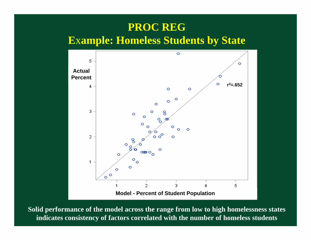
PROC REGExample: Homeless Students by State

Solid performance of the model across the range from low to high homelessness states indicates consistency of factors correlated with the number of homeless students

r2=.652

ActualPercent

Model - Percent of Student Population

Special Data Needs: Problems with OutliersPROC ROBUSTREG


• Robust regression is achieved by identifying outliers and limiting their influence by assigning weights and then performing standard regression

• Supports outlier detection using M, LTS, S and MM estimation; robust ANOVA

• Provides robust R2 and deviance, robust modeling parameters and outlier diagnostics

PROC ROBUSTREGExample: Log-Log Regression With Weighted Outliers

SAS/STAT® 9.2 User’s Guide, support.sas.com

In ROBUSTREG, the outliers are not disregarded: weights are assigned and incorporated in the regression

Special Data Needs: Ill-Conditioned DataPROC ORTHOREG


• Regression using the Gentleman-Givens procedure instead of collecting crossproducts

• For ill-conditioned data, where small errors in the data may cause large errors in the results – more accurate than PROG REG or GLM

• “ORTHO” in ORTHOREG refers to using an orthogonal approach to Least Squares, notorthogonal regression

PROC ORTHOREGExample: Fitting a Higher-Order Polynomial

SAS/STAT® 9.2 User’s Guide, support.sas.com

An example of ORTHOREG fitting a 9th-degree polynomial, where near singularities must be distinguished from true ones

Special Data Needs: TransformationPROC TRANSREG


• Regression with a number of data transformations, including smooth, spline, Box-Cox and other non-linear forms

• Supports fitting splines with a user-specified degree and number of knots; works for piece-wise and discontinuous solutions

• Also supports variable transformation for canonical regression and response surface regression

PROC TRANSREGExample: Spline Regression to a Complex Form

TRANSREG used to fit splines to a spectrographic line profileto determine the radial velocity of erupting gas from a star

Special Model Types: General LinearPROC GLM


• General purpose procedure for continuous least squares regression using classification predictor variables as well as continuous

• No Bayesian capability at this time; use GENMOD or MCMC for Bayesian functionality

• While capable of many types of models and analysis, another procedure is often better for a specific task

PROC GLMExample: Age Group as a Categorical Predictor Variable

GLM used with ODS Graphics to visualize statistical output

An Overview of ODS Statistical Graphics in SAS® 9.3Robert N. Rodriguez, SAS Institute Inc., Cary, NC

agegroup

Distribution of Response

Special Model Types: Quantile RegressionPROC QUANTREG


• Quantile regression: while other procedures model the mean, quantile regression models the median and other specified quantiles to provide a more complete picture of the response variable

• Uncertainties for individual quantiles can be estimated by bootstrapping

• Model fitting by Least Squares

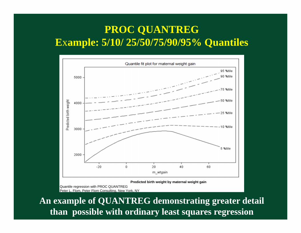
PROC QUANTREGExample: 5/10/ 25/50/75/90/95% Quantiles

An example of QUANTREG demonstrating greater detail than possible with ordinary least squares regression

Quantile regression with PROC QUANTREGPeter L. Flom, Peter Flom Consulting, New York, NY

Predicted birth weight by maternal weight gain

Special Model Types: PSL, PCA RegressionPROC PLS


• Special procedure for Partial Least Squares and Principal Component regression: predictor and response variables are projected into a new coordinate systems, possibly with reduced complexity

• Supports reduced rank regression with cross validation of the number of components; no Bayesian capability at this time

• After projection, model fitting is by Least Squares

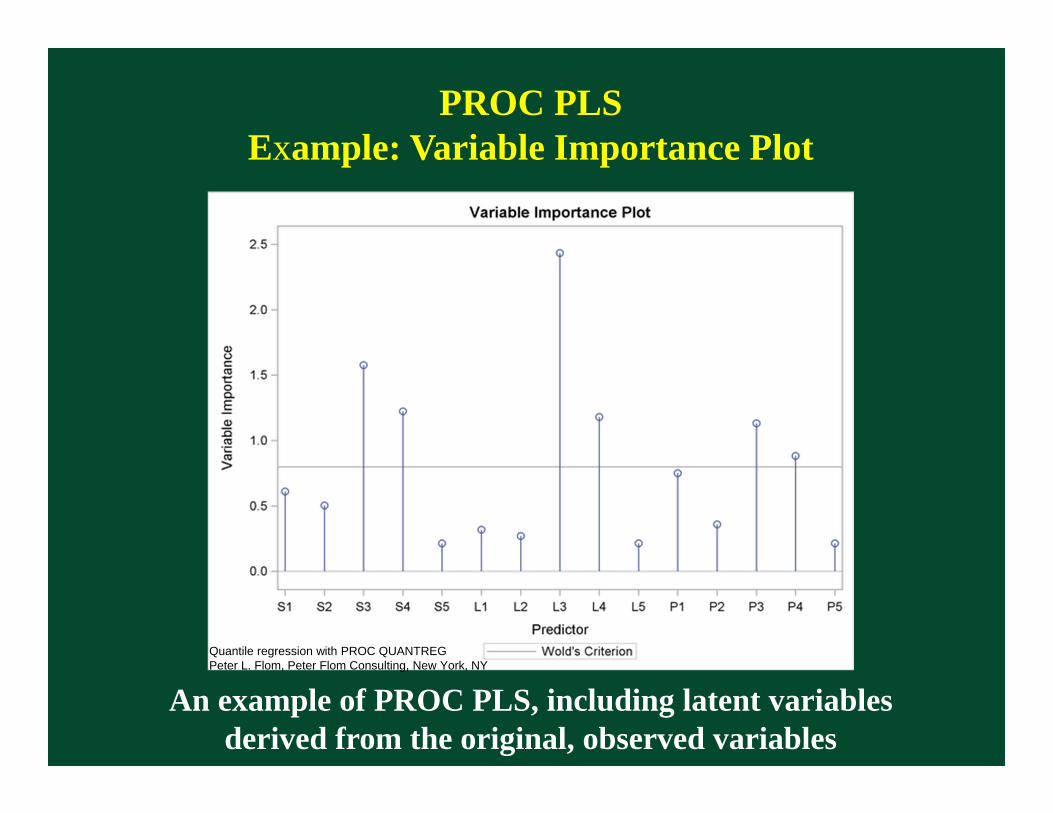
PROC PLSExample: Variable Importance Plot

An example of PROC PLS, including latent variablesderived from the original, observed variables

Quantile regression with PROC QUANTREGPeter L. Flom, Peter Flom Consulting, New York, NY

Special Model Types: Survey DataPROC SURVEYREG


• Special capabilities for analysis in the presence of common survey data features, including stratification, clustering and weighting

• Supports estimation of sampling error using either Taylor series or primary sample units

• Model fitting by Generalized Least Squares

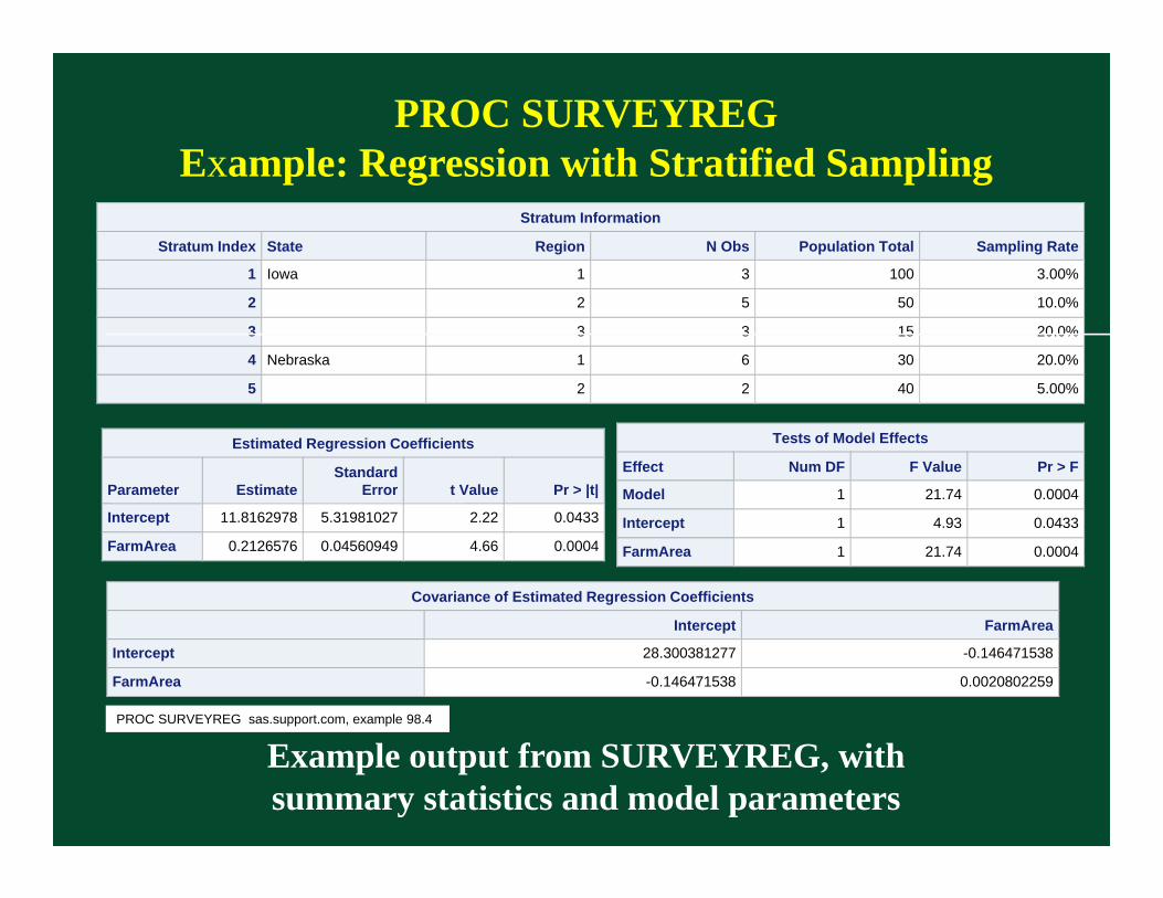
PROC SURVEYREGExample: Regression with Stratified Sampling

Example output from SURVEYREG, withsummary statistics and model parameters

PROC SURVEYREG sas.support.com, example 98.4

Stratum Information

Stratum Index State Region N Obs Population Total Sampling Rate

1 Iowa 1 3 100 3.00%

2 2 5 50 10.0%

3 3 3 15 20.0%

4 Nebraska 1 6 30 20.0%

5 2 2 40 5.00%

Tests of Model Effects

Effect Num DF F Value Pr > F

Model 1 21.74 0.0004

Intercept 1 4.93 0.0433

FarmArea 1 21.74 0.0004

Note: The denominator degrees of freedom for the F tests is 14.

Estimated Regression Coefficients

Parameter EstimateStandard

Error t Value Pr > |t|

Intercept 11.8162978 5.31981027 2.22 0.0433

FarmArea 0.2126576 0.04560949 4.66 0.0004

Covariance of Estimated Regression Coefficients

Intercept FarmArea

Intercept 28.300381277 -0.146471538

FarmArea -0.146471538 0.0020802259

Special Model Types: Survey DataPROC SURVEYPHREG


• Performs Cox Proportional Hazards modeling on survey data with truncation, supporting stratification, clustering and weighting

• Performs estimation of variance by model parameters by Taylor series, BRR or Jackknife

• Model fitting by Maximum Likelihood

PROC SURVEYREGExample: Stratified Sampling with Truncated Data

Example output from SURVEYPHREG, withsummary statistics and model parameters

PROC SURVEYPHREG sas.support.com, example 97.2

Analysis of Maximum Likelihood Estimates

Parameter DF Estimate Standard Error t Value Pr > |t|Hazard

Ratio

BodyWeight 586 0.011920 0.003155 3.78 0.0002 1.012

Smoke -1 586 -1.174048 0.739450 -1.59 0.1129 0.309

Smoke 1 586 -1.006515 0.578810 -1.74 0.0826 0.365

Smoke 2 586 -0.674183 0.558412 -1.21 0.2278 0.510

Smoke 3 586 0 . . . 1.000

Type III Tests of Model Effects

Effect Num DF Den DF F Value Pr > F

BodyWeight 1 586 14.27 0.0002

Smoke 3 586 1.49 0.2160

Estimate

Label Estimate Standard Error DF t Value Pr > |t| Exponentiated

Row 1 -0.7532 0.3870 586 -1.95 0.0521 0.4709

Special Model Types:Contingency Table Regression

PROC CATMOD


• A generalization of continuous methods to categorical data, performs linear regression and other analyses on data than can be expressed in a contingency tables

• Supports both ordinary and logistic regression, log-linear and repeated measures

• Model fitting by WLS; ML is available for log-linear and generalized logit models

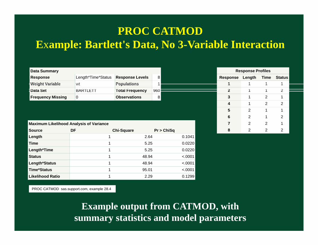
PROC CATMODExample: Bartlett's Data, No 3-Variable Interaction

Example output from CATMOD, withsummary statistics and model parameters

PROC CATMOD sas.support.com, example 28.4

Data SummaryResponse Length*Time*Status Response Levels 8Weight Variable wt Populations 1Data Set BARTLETT Total Frequency 960Frequency Missing 0 Observations 8

Response ProfilesResponse Length Time Status

1 1 1 12 1 1 23 1 2 14 1 2 25 2 1 16 2 1 27 2 2 18 2 2 2

Maximum Likelihood Analysis of VarianceSource DF Chi-Square Pr > ChiSqLength 1 2.64 0.1041Time 1 5.25 0.0220Length*Time 1 5.25 0.0220Status 1 48.94 <.0001Length*Status 1 48.94 <.0001Time*Status 1 95.01 <.0001Likelihood Ratio 1 2.29 0.1299

Special Model Types: Response SurfacePROC RSREG


• Creates a quadratic Response Surface, a general linear model where optimal solutions are identified as peaks or valleys, with ridge analysis to identify regions near optimal responses

• Relies on ODS graphic to display the response surface, ridges and fit parameters

• Model fitting by Least Squares

PROC RSREGExample: Response Surface with a Single Solution

An example of RSREG, with the optimal solution found atthe minimum; multiple minima and maxima are possible

http://v8doc.sas.com/sashtml/stat/chap56/sect5.htm

Response Surface with a Simple Optimum

Special Model Types: Survival AnalysisPROC LIFEREG


• Models time to failure data as a linear combination of predictors and a random disturbance term, which can be described by many different distributions

• Supports standard survival analysis data censored on the right, left, both or neither; has a Bayesian option

• Model fitting by Least Squares, only one model statement per procedure

PROC LIFEREGExample: Cumulative Hazard Model

This example of LIFEREG plots the log-logisticvs. the Kaplan-Meier Cumulative Hazard

Response Surface with a Simple Optimum

D. Hosmer and S. LemeshowApplied Survival Analysis, Ch. 8

Special Model Types: Proportional HazardsPROC PHREG


• Cox Proportional Hazards modeling, where the a unit increase in a predictor multiplies the risk by a factor determined by the model

• Supports proportional hazards models with data censored on the right, left, both or neither, variable selection by forwards, backwards, stepwise or best subset

• Maximum Likelihood with a Bayesian option

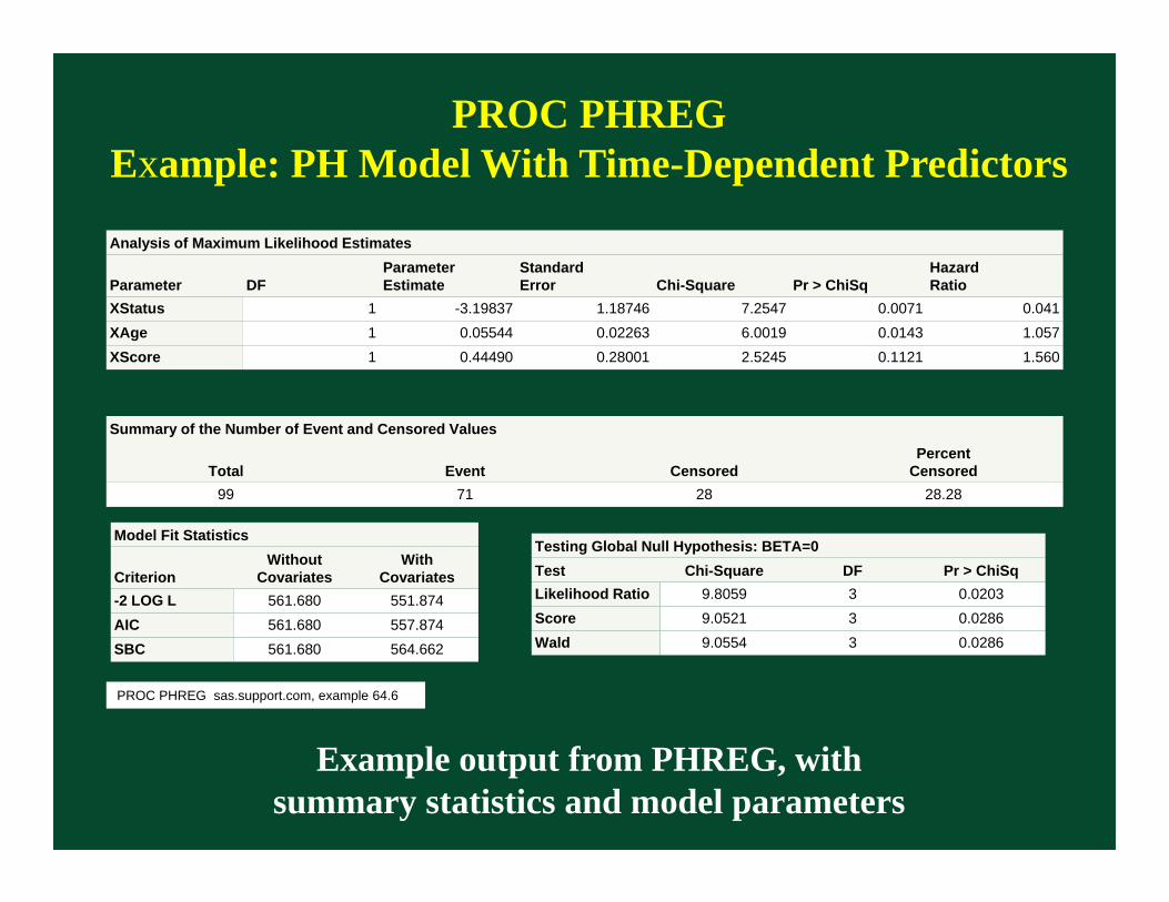
PROC PHREGExample: PH Model With Time-Dependent Predictors

Example output from PHREG, withsummary statistics and model parameters

PROC PHREG sas.support.com, example 64.6

Summary of the Number of Event and Censored Values

Total Event CensoredPercent

Censored99 71 28 28.28

Model Fit Statistics

CriterionWithout

CovariatesWith

Covariates-2 LOG L 561.680 551.874AIC 561.680 557.874SBC 561.680 564.662

Testing Global Null Hypothesis: BETA=0Test Chi-Square DF Pr > ChiSqLikelihood Ratio 9.8059 3 0.0203Score 9.0521 3 0.0286Wald 9.0554 3 0.0286

Analysis of Maximum Likelihood Estimates

Parameter DFParameterEstimate

StandardError Chi-Square Pr > ChiSq

HazardRatio

XStatus 1 -3.19837 1.18746 7.2547 0.0071 0.041XAge 1 0.05544 0.02263 6.0019 0.0143 1.057XScore 1 0.44490 0.28001 2.5245 0.1121 1.560

Special Model Types: Structural EquationsPROC CALIS


• In Structural Equation Modeling, a linear combination of predictors describes a vector equal to a linear combination of outcome variables

• Supports latent variables, multiple and multivariate regression, path analysis and canonical correlation

• Maximum Likelihood with Least Squares and Bayesian options

PROC CALISExample: Linear Relations among Factor Loadings

Example output from CALIS, withmatrices of model parameters

PROC CALIS sas.support.com, example 25.4

Estimated Parameter Matrix B[6:2]General Matrix

Fact1 Fact2var1 0.3422 0.6318

[b11]var2 0.321 0.6531

[b21]var3 0.4918 0.4822

[b31]var4 0.5755 0.3985

[b41]var5 0.7769 0.1971

[b51]var6 0.6666 0.3074

[b61]

Estimated Parameter Matrix D[6:6]Diagonal Matrix

var1 var2 var3 var4 var5 var6var1 1.0077 0 0 0 0 0

[d1]var2 0 0.9971 0 0 0 0

[d2]var3 0 0 0.9908 0 0 0

[d3]var4 0 0 0 0.9909 0 0

[d4]var5 0 0 0 0 0.9964 0

[d5]var6 0 0 0 0 0 1.0169

[d6

Discrete Outcomes: Logistic RegressionPROC LOGISTIC

• Regression Type: binary & ordinal outcomes, linear

• General procedure for logistic regression with a number of options; other procedures may offer more capabilities for specific types of discrete models

• Supports many model variable selection methods and diagnostic tests


Discrete Outcomes: General Linear ModelsPROC GENMOD

• Regression Type: discrete outcomes, linear

• Generalized linear models with discrete outcomes, appropriate where the data are not normally distributed or the variance is not the same for all observations

• Supports Poisson Regression and Repeated Measures

• Model fitting by Maximum Likelihood with a Bayesian option

Discrete Outcomes: PROBIT ModelsPROC PROBIT

• Regression Type: discrete outcomes, linear

• Generalized linear models with discrete outcomes, appropriate for use with discrete event data

• Supports probit, logit, ordinal logistic, and extreme value / gompit

• Model fitting by Maximum Likelihood; no Bayesian option at this time

Discrete Outcomes: Survey DataPROC SURVEYLOGISTIC

• Regression Type: binary & ordinal outcomes, linear

• Performs regression on survey data with categorical responses; special capabilities for analysis for common survey data features, including stratification, clustering and weighting

• Supports estimation of sampling error using either Taylor series or resampling


Non-Linear Models: GeneralPROC NLIN

• Regression Type: non-linear

• Performs non-linear regression with the dependent variable divided into a mean component and a (random) error component; process is iterative

• Supports steepest-descent, Newton, modified Gauss-Newton and Marquardt methods

• Model fitting by Least Squares or WLS

PROC NLINExample: Fitting a Model to a Complex Curve

In this example of NLIN, observations are normally distributed about a non-linear function – in this case, a Morlet wavelet

Non-Linear Models: MixedPROC NLMIXED

• Regression Type: non-linear

• Performs non-linear regression where both the mean and errors components of the dependent variable are non-linear; process uses a Taylor series expansion about zero

• Supports normal, binomial and Poisson distributions and capability for programing a general distribution

• Likelihood-based model fitting

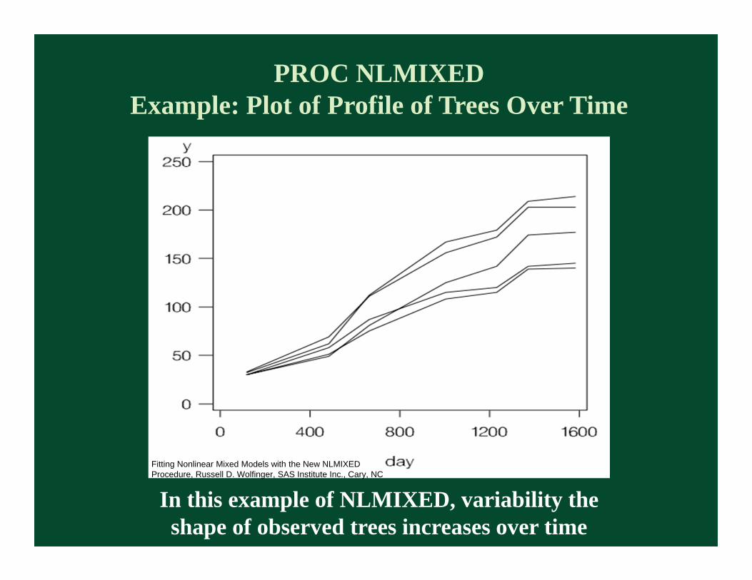
PROC NLMIXEDExample: Plot of Profile of Trees Over Time

In this example of NLMIXED, variability theshape of observed trees increases over time

Fitting Nonlinear Mixed Models with the New NLMIXEDProcedure, Russell D. Wolfinger, SAS Institute Inc., Cary, NC

Linear Mixed: Fixed and Random EffectsPROC MIXED

• Regression Type: linear, fixed and random effects

• Performs linear regression using a linear combination of fixed effects added to a second linear combination of random effects

• Support repeated measures in longitudinal studies, Especially useful for dealing with missing data


PROC MIXEDExample: Repeated Measures

Example of MIXED, incorporating both fixed and randomeffects to improve the predictive power of the model

Repeated Measures Modeling With PROC MIXED E. Barry Moser, Louisiana State University, Baton Rouge, LA

Actual Growth of Sitka Spruce trees Predicted Growth with Random Coefficient Asymptote

Linear Mixed: General Mixed Models:PROC GLIMMIX

• Regression Type: linear mixed

• A generalization of GENMOD and MIXED to permit normally-distributed random effects and non-normal error terms, fitting models to correlated data or where the variability is not constant

• Supports a wide variety of distributions and link functions


PROC GLIMMIXExample: Crossed Random Effects

LOESS with crossed random effects analyzes in-breeding in an isolated population, allowing generalization to all populations

PROC GLIMMIX sas.support.com, example 38.2

Non-Parametric: Local RegressionPROC LOESS

• Regression Type: linear, non-parametric

• Develops a model using non-parametric regression to segments of data and calculates confidence limits for the outcome; computationally intensive

• Supports multiple dependent variables, multidimensional predictors and interpolation using kd trees

• Model fitting by local least squares

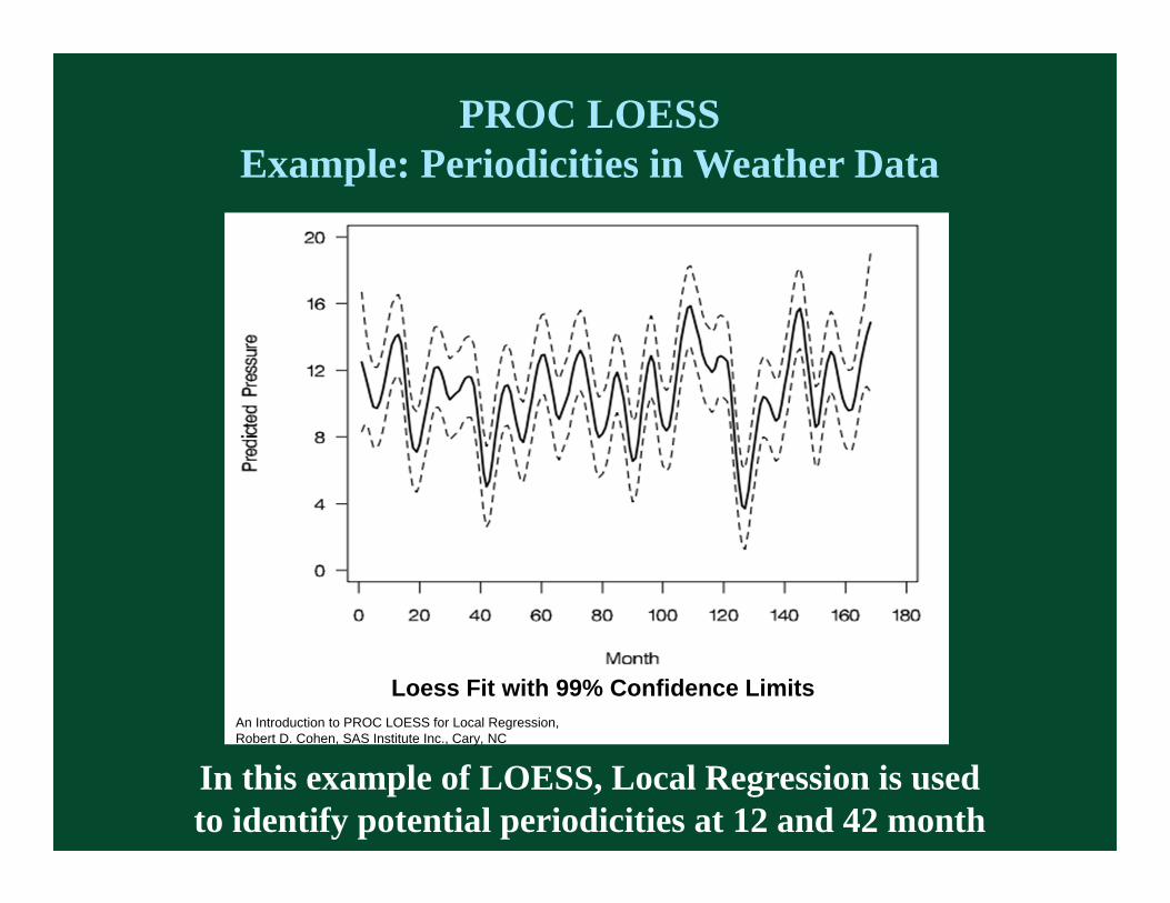
PROC LOESSExample: Periodicities in Weather Data

In this example of LOESS, Local Regression is usedto identify potential periodicities at 12 and 42 month

Loess Fit with 99% Confidence LimitsAn Introduction to PROC LOESS for Local Regression, Robert D. Cohen, SAS Institute Inc., Cary, NC

Non-Parametric: Additive ModelsPROC GAM

• Regression Type: linear, non-parametric

• General Additive Models, with multiple independent non-parametric predictors; univariate smoothing provides finer details than is possible with the piece-wise LOESS procedure

• Supports non-parametric and semi-paramentricmodels, multidimensional predictors

• Model fitting by iterative reweighted least squares

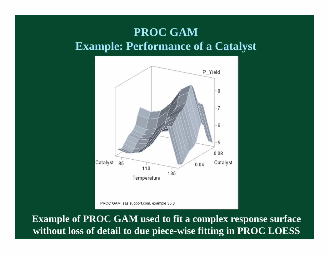
PROC GAMExample: Performance of a Catalyst

Example of PROC GAM used to fit a complex response surface without loss of detail to due piece-wise fitting in PROC LOESS

PROC GAM sas.support.com, example 36.3

Questions

David J. [email protected]

[email protected]

NON-LINEARLINEAR MIXED

NON-PARAMETRIC

Speed Dating with SAS Regression · PDF fileSpeed Dating with SAS Regression Procedures David...

Documents

Transcript of Speed Dating with SAS Regression · PDF fileSpeed Dating with SAS Regression Procedures David...