Paper presented at the IEEE International Ultrasonics Symposium, Prague, Czech Republic, 2013:

Spectral Velocity Estimation in the Transverse Direction

Jørgen Arendt Jensen

Center for Fast Ultrasound Imaging,Biomedical Engineering group, Department of Electrical Engineering, Bldg. 349,Technical University of Denmark, DK-2800 Kgs. Lyngby, Denmark

To be published in Proceedings of IEEE International Ultrasonics Symposium, Prague, Czech Republic, 2013.

Spectral Velocity Estimation in theTransverse Direction

Jørgen Arendt Jensen

Center for Fast Ultrasound Imaging, Department of Electrical Engineering,Technical University of Denmark, DK-2800 Lyngby, Denmark

Abstract—A method for estimating the velocity spectrum for afully transverse flow at a beam-to-flow angle of 90◦is described.The approach is based on the Transverse Oscillation (TO)method, where an oscillation across the ultrasound beam is madeduring receive processing. A fourth-order estimator based on thecorrelation of the received signal is derived. A Fourier transformof the correlation signal yields the velocity spectrum. Performingthe estimation for short data segments gives the velocity spectrumas a function of time as for ordinary spectrograms, and italso works for a beam-to-flow angle of 90◦. The approach isvalidated using Field II simulations. A 3 MHz convex arraywith lambda pitch is modeled. The transmit focus is at 200mm and 2 times 32 elements are used in receive. A dual-peakHamming apodization with a spacing of 96 elements betweenthe peaks is used during receive beamforming for creating thelateral oscillation. Pulsatile flow in a femoral artery placed 40mm from the transducer is simulated for one cardiac cycleusing the Womersly-Evan’s flow model. The bias of the meanestimated frequency is 13.6% compared to the true velocity andthe mean relative std is 14.3%. This indicates that the newestimation scheme can reliably find the spectrum at 90◦, wherea traditional estimator yields zero velocity. Measurements havebeen conducted with the SARUS experimental scanner and a BK8820e convex array transducer (BK Medical, Herlev, Denmark).A CompuFlow 1000 (Shelley Automation, Inc, Toronto, Canada)generated the artificial femoral artery flow in the phantom. It isdemonstrated that the transverse spectrum can be found from themeasured data. The estimated spectra degrade when the angleis different from 90◦, but are usable down to 60-70◦. Below thisangle the traditional spectrum is best and should be used. Theconventional approach can automatically be corrected for anglesfrom 0-70◦to give a fully quantitative velocity spectrum withoutoperator intervention.

I. INTRODUCTION

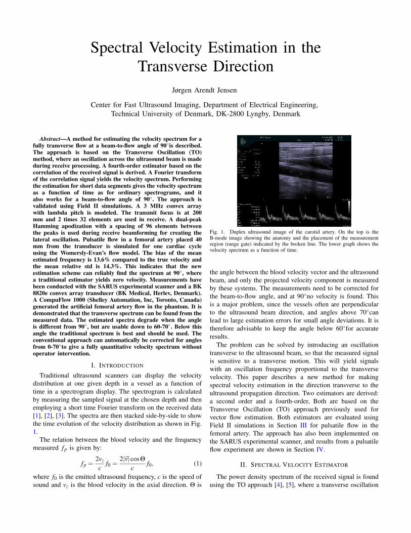
Traditional ultrasound scanners can display the velocitydistribution at one given depth in a vessel as a function oftime in a spectrogram display. The spectrogram is calculatedby measuring the sampled signal at the chosen depth and thenemploying a short time Fourier transform on the received data[1], [2], [3]. The spectra are then stacked side-by-side to showthe time evolution of the velocity distribution as shown in Fig.1.

The relation between the blood velocity and the frequencymeasured fp is given by:

fp =2vz

cf0 =

2|~v|cosΘc

f0, (1)

where f0 is the emitted ultrasound frequency, c is the speed ofsound and vz is the blood velocity in the axial direction. Θ is

Fig. 1. Duplex ultrasound image of the carotid artery. On the top is theB-mode image showing the anatomy and the placement of the measurementregion (range gate) indicated by the broken line. The lower graph shows thevelocity spectrum as a function of time.

the angle between the blood velocity vector and the ultrasoundbeam, and only the projected velocity component is measuredby these systems. The measurements need to be corrected forthe beam-to-flow angle, and at 90◦no velocity is found. Thisis a major problem, since the vessels often are perpendicularto the ultrasound beam direction, and angles above 70◦canlead to large estimation errors for small angle deviations. It istherefore advisable to keep the angle below 60◦for accurateresults.

The problem can be solved by introducing an oscillationtransverse to the ultrasound beam, so that the measured signalis sensitive to a transverse motion. This will yield signalswith an oscillation frequency proportional to the transversevelocity. This paper describes a new method for makingspectral velocity estimation in the direction transverse to theultrasound propagation direction. Two estimators are derived:a second order and a fourth-order, Both are based on theTransverse Oscillation (TO) approach previously used forvector flow estimation. Both estimators are evaluated usingField II simulations in Section III for pulsatile flow in thefemoral artery. The approach has also been implemented onthe SARUS experimental scanner, and results from a pulsatileflow experiment are shown in Section IV.

II. SPECTRAL VELOCITY ESTIMATOR

The power density spectrum of the received signal is foundusing the TO approach [4], [5], where a transverse oscillation

is introduced during the receive beamforming. Two image linesare focused in parallel, where the left one contains the in-phaseand the right the quadrature component. This complex signalcan, at one fixed depth, be described by [6]:

rsq(i) = cos(2π fpiTpr f )exp( j2π fxiTpr f ), (2)

where i is the emission number, Tpr f is the pulse repetitionperiod and fp is the received axial frequency given by (1).fx is the transverse oscillation frequency and is equal to tovx/λx, where λx is the transverse oscillation period and vx thetransverse velocity. The temporal Hilbert transform of (2) is

rsqh(i) = sin(2π fpiTpr f )exp( j2π fxiTpr f ). (3)

Combining (2) and (3) and using Euler’s equations gives

rsq(i) =12(exp( j2πiTpr f ( fx + fp))+ exp( j2πiTpr f ( fx − fp)))

rsqh(i) =12 j

(exp( j2πiTpr f ( fx + fp))− exp( j2πiTpr f ( fx − fp))) .

Two new signals are then formed from:

r1(i) = rsq(i)+ jrsqh(i) = exp( j2πiTpr f ( fx + fp)) (4)r2(i) = rsq(i)− jrsqh(i) = exp( j2πiTpr f ( fx − fp)). (5)

The power density spectrum of a stochastic signal is foundfrom:

P11( f ) =+∞

∑k=−∞

R11(k)exp(− j2π f k), (6)

where R11(k) is the autocorrelation of the received signal. Forthe transverse velocity component this can be derived from thecross-correlation function R12(k) between the spatial in-phaseand quadrature signal given as:

R12(k) =+∞

∑i=−∞

r1(i)r2(i+ k)

=+∞

∑i=−∞

exp( j2πiTpr f ( fx + fp))

×exp( j2π(i+ k)Tpr f ( fx − fp))

= exp( j2πkTpr f ( fx − fp))+∞

∑i=−∞

exp( j2πiTpr f 2 fx)

= exp( j2πkTpr f fp)×+∞

∑i=−∞

exp( j2πk(i+ k)Tpr f fx)exp( j2πiTpr f fx)

= exp(− j2πkTpr f fp)R11(k). (7)

The frequency fp is zero in the case there is no axial velocitycomponent (vz = 0) and the cross-correlation directly equalsthe autocorrelation of the transverse signal. Making a shortFourier transform of this, thus, directly reveals the transversevelocity spectrum. This is called the second order estimator.

The compensation for the axial velocity can also be madeusing a fourth-order estimator similar to the one derived in

[6]. The fourth order correlation function is calculated as:

R11(k) =+∞

∑i=−∞

r1(i)r∗1(i+ k),

R22(k) =+∞

∑i=−∞

r2(i)r∗2(i+ k)

R44(k) = R11(k) ·R22(k), (8)

which eliminates the axial component. An elimination of thelateral component can be done using:

R44ax(k) = R11(k) ·R∗22(k). (9)

The spectrum is then found from:

P44( f ) =+∞

∑k=−∞

R44(k)exp(− j2π f k). (10)

This approach is called the fourth-order method.

III. SIMULATION OF TO DATA AND RESULTS

Blood flow in the femoral artery has been simulated usingField II [7], [8] and the Womersley-Evans’ pulsatile flowmodel [9], [2]. The model gives realistic simulated velocityprofiles for a normal human geometry [10]. A 3 MHz convexarray transducer with 128 active elements has been used.The center 64 elements are used in transmit, and the outer64 elements are used during receive. The TO field has beenoptimized for imaging at 40 mm by adjusting the time delaysand apodization function [11].

The resulting spectra for the second order method is shownin Fig. 2 for a beam-to-flow angle of 90◦(top) and 60◦(bottom).The solid green curve shows the peak velocity at the centerof the vessel. The spectrum can be estimated at 90◦with somebias, but both positive and negative velocities are shown. At60◦the modulation from the term exp(− j2πkTpr f fp) in (7) setsin and severely distorts the spectrum, thus, making is uselessfor quantitative studies.

The resulting power density spectrograms for different an-gles for the fourth-order methods are shown in Fig. 3. It isseen that the spectrogram can reliably be estimated for fullytransverse flow. The estimates get progressively worse whenthe beam-to-flow angle deviates from 90◦as shown in Fig. 4 for60◦. The transverse velocity spectra is considerably widenedand gets less accurate. This is not a major problem as theaxial velocity spectrum now is a reliable measure of velocitydistribution. For angles lower than 60◦the normal spectrogramcan be used and gives a good estimate. The angle can easilybe estimated from the TO data measured for the spectralestimation and be used for selecting the spectrum to display.It can also automatically adjust the velocity axis for the axialvelocity spectrum.

The mean velocity for the fourth-order spectrum has beencalculated and is shown as the blue curve in Fig. 5 as a functionof time. The corresponding true mean velocity is shown also.The bias relative to peak velocity in the vessel is 13.6% (0.18m/s) and the relative std. is 0.19 m/s (14.2%).

2

Vel

ocity

[m/s

]

Time

Second order method at 90 degrees

0 0.1 0.2 0.3 0.4 0.5 0.6 0.7 0.8 0.9−1.5

−1

−0.5

0

0.5

1

1.5

2

Vel

ocity

[m/s

]

Time [s]

Axial spectrum at 90 degrees

0 0.1 0.2 0.3 0.4 0.5 0.6 0.7 0.8 0.9

−1

0

1

2

Vel

ocity

[m/s

]

Time

Second order method at 60 degrees

0 0.1 0.2 0.3 0.4 0.5 0.6 0.7 0.8 0.9−1.5

−1

−0.5

0

0.5

1

1.5

2

Vel

ocity

[m/s

]

Time [s]

Axial spectrum at 60 degrees

0 0.1 0.2 0.3 0.4 0.5 0.6 0.7 0.8 0.9

−1

0

1

2

Fig. 2. Estimated power density spectrograms for the second order methodfor a simulated femoral artery. The lateral (top) and axial velocities (bottom)are shown for 90◦(top) and 60◦(bottom) flow angles.

IV. FLOW RIG MEASUREMENTS

Measurements have been made using the SARUS exper-imental ultrasound scanner [12] connected to a BK 8820e(BK Medical, Herlev, Denmark) convex array probe. A duplexsequence was employed with B-mode and TO emissionsinterleaved with a pulse repetition frequency of 5 kHz. Theflow lines were emitted with the center of the aperture andfocused straight down. The probe was operated at 3 MHz and64 elements was during transmit that was focused at 105 mm(F# of 5). The received signal of all 192 transducer elementswas sampled at 17.5 MHz with 12 bits precision. The two TObeams were focused using the center 96 elements and two vonHann apodization peaks each with a width of 32 elements andtheir peaks separated by 64 elements. The lateral wavelengthλx was set to 0.88 mm for the focusing.

The flow was generated by a CompuFlow 1000 (ShelleyAutomation, Inc, Toronto, Canada) connected to a dedicatedcarotid bifurcation phantom (Danish Phantom Design, Fred-erikssund, Denmark). filled with Shelley Blood MimickingFluid for ultrasound (BMF-3L-US, Shelley Automation, Inc,Toronto, Canada). The 8 mm diameter straight tube entranceto the bifurcation was used as the measurement site. The pumpwas set to use the femoral waveform to mimic the waveformfound in the femoral artery with both positive and negative

Vel

ocity

[m/s

]

Time [s]

Fourth order method at 90 degrees

0 0.1 0.2 0.3 0.4 0.5 0.6 0.7 0.8 0.9−1.5

−1

−0.5

0

0.5

1

1.5

2

Vel

ocity

[m/s

]

Time [s]

Axial spectrum at 90 degrees

0 0.1 0.2 0.3 0.4 0.5 0.6 0.7 0.8 0.9

−1

0

1

2

Vel

ocity

[m/s

]

Time [s]

Fourth order method at 75 degrees

0 0.1 0.2 0.3 0.4 0.5 0.6 0.7 0.8 0.9−1.5

−1

−0.5

0

0.5

1

1.5

2

Vel

ocity

[m/s

]

Time [s]

Axial spectrum at 75 degrees

0 0.1 0.2 0.3 0.4 0.5 0.6 0.7 0.8 0.9

−1

0

1

2

Fig. 3. Estimated power density spectrograms for the fourth-order methodfor a simulated femoral artery. The lateral (top) and axial velocities (bottom)are shown for 90◦(top) and 75◦(bottom) flow angles.

Vel

ocity

[m/s

]

Time [s]

Fourth order method at 60 degrees

0 0.1 0.2 0.3 0.4 0.5 0.6 0.7 0.8 0.9−1.5

−1

−0.5

0

0.5

1

1.5

2

Vel

ocity

[m/s

]

Time [s]

Axial spectrum at 60 degrees

0 0.1 0.2 0.3 0.4 0.5 0.6 0.7 0.8 0.9

−1

0

1

2

Fig. 4. Estimated power density spectrograms for the fourth-order methodfor a simulated femoral artery. The lateral (top) and axial velocities (bottom)are shown for a 60◦flow angle.

3

0 0.1 0.2 0.3 0.4 0.5 0.6 0.7 0.8 0.9 1−1

−0.5

0

0.5

1

1.5

Vel

ocity

[m/s

]

Time [s]

True and mean velocity from fourth order spectrum at 0 degrees

True mean velocityMean velocity from spectrum

Fig. 5. Estimated mean velocity for fourth-order spectrum compared to truemean velocity for 90◦.

Vel

ocity

[m/s

]

Time [s]

Fourth order method at 90 degrees

0 0.5 1 1.5 2 2.5−0.1

−0.05

0

0.05

0.1

0.15

0.2

Fig. 6. Measured fourth-order spectrum for pulsatile flow mimicking thatfound in the femoral artery.

velocities. The peak volume flow was set to 10 mL/s, and thebeam to flow angle was estimated to be 91.0◦± 3.3◦from thevelocity data.

Data were acquired continuously for 3 seconds yielding 3.8Gbytes of fully sampled RF data. It was beamformed andthe fourth-order estimator was used on the focused TO data.The resulting fourth-order spectrum found at the center of thevessel is shown in Fig. 6 for three seconds. Four peaks in thesystolic phases can be seen in the data with a positive velocityfollowed by negative velocities in the diastole as expected. Thepeak velocity is fairly low due to limitations in the setup.

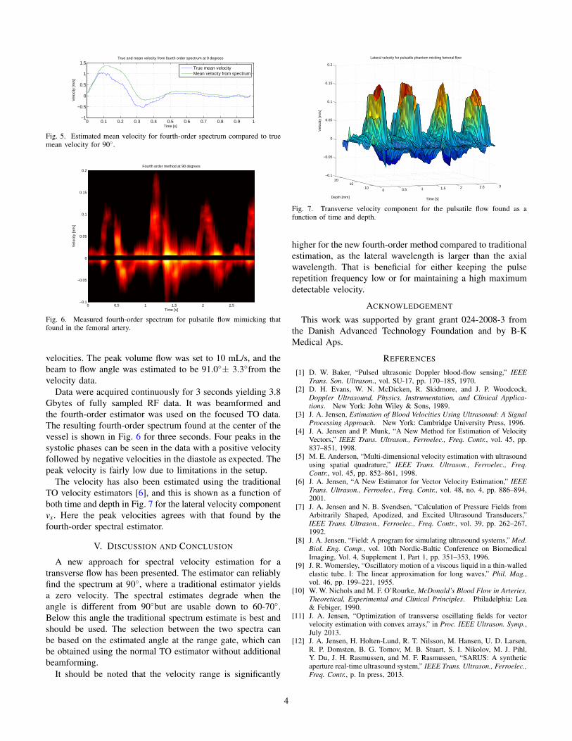
The velocity has also been estimated using the traditionalTO velocity estimators [6], and this is shown as a function ofboth time and depth in Fig. 7 for the lateral velocity componentvx. Here the peak velocities agrees with that found by thefourth-order spectral estimator.

V. DISCUSSION AND CONCLUSION

A new approach for spectral velocity estimation for atransverse flow has been presented. The estimator can reliablyfind the spectrum at 90◦, where a traditional estimator yieldsa zero velocity. The spectral estimates degrade when theangle is different from 90◦but are usable down to 60-70◦.Below this angle the traditional spectrum estimate is best andshould be used. The selection between the two spectra canbe based on the estimated angle at the range gate, which canbe obtained using the normal TO estimator without additionalbeamforming.

It should be noted that the velocity range is significantly

0 0.5 1 1.5 2 2.5 31015

20−0.1

−0.05

0

0.05

0.1

0.15

0.2

Time [s]

Lateral velocity for pulsatile phantom micking femoral flow

Depth [mm]

Vel

ocity

[m/s

]

Fig. 7. Transverse velocity component for the pulsatile flow found as afunction of time and depth.

higher for the new fourth-order method compared to traditionalestimation, as the lateral wavelength is larger than the axialwavelength. That is beneficial for either keeping the pulserepetition frequency low or for maintaining a high maximumdetectable velocity.

ACKNOWLEDGEMENT

This work was supported by grant grant 024-2008-3 fromthe Danish Advanced Technology Foundation and by B-KMedical Aps.

REFERENCES

[1] D. W. Baker, “Pulsed ultrasonic Doppler blood-flow sensing,” IEEETrans. Son. Ultrason., vol. SU-17, pp. 170–185, 1970.

[2] D. H. Evans, W. N. McDicken, R. Skidmore, and J. P. Woodcock,Doppler Ultrasound, Physics, Instrumentation, and Clinical Applica-tions. New York: John Wiley & Sons, 1989.

[3] J. A. Jensen, Estimation of Blood Velocities Using Ultrasound: A SignalProcessing Approach. New York: Cambridge University Press, 1996.

[4] J. A. Jensen and P. Munk, “A New Method for Estimation of VelocityVectors,” IEEE Trans. Ultrason., Ferroelec., Freq. Contr., vol. 45, pp.837–851, 1998.

[5] M. E. Anderson, “Multi-dimensional velocity estimation with ultrasoundusing spatial quadrature,” IEEE Trans. Ultrason., Ferroelec., Freq.Contr., vol. 45, pp. 852–861, 1998.

[6] J. A. Jensen, “A New Estimator for Vector Velocity Estimation,” IEEETrans. Ultrason., Ferroelec., Freq. Contr., vol. 48, no. 4, pp. 886–894,2001.

[7] J. A. Jensen and N. B. Svendsen, “Calculation of Pressure Fields fromArbitrarily Shaped, Apodized, and Excited Ultrasound Transducers,”IEEE Trans. Ultrason., Ferroelec., Freq. Contr., vol. 39, pp. 262–267,1992.

[8] J. A. Jensen, “Field: A program for simulating ultrasound systems,” Med.Biol. Eng. Comp., vol. 10th Nordic-Baltic Conference on BiomedicalImaging, Vol. 4, Supplement 1, Part 1, pp. 351–353, 1996.

[9] J. R. Womersley, “Oscillatory motion of a viscous liquid in a thin-walledelastic tube. I: The linear approximation for long waves,” Phil. Mag.,vol. 46, pp. 199–221, 1955.

[10] W. W. Nichols and M. F. O’Rourke, McDonald’s Blood Flow in Arteries,Theoretical, Experimental and Clinical Principles. Philadelphia: Lea& Febiger, 1990.

[11] J. A. Jensen, “Optimization of transverse oscillating fields for vectorvelocity estimation with convex arrays,” in Proc. IEEE Ultrason. Symp.,July 2013.

[12] J. A. Jensen, H. Holten-Lund, R. T. Nilsson, M. Hansen, U. D. Larsen,R. P. Domsten, B. G. Tomov, M. B. Stuart, S. I. Nikolov, M. J. Pihl,Y. Du, J. H. Rasmussen, and M. F. Rasmussen, “SARUS: A syntheticaperture real-time ultrasound system,” IEEE Trans. Ultrason., Ferroelec.,Freq. Contr., p. In press, 2013.

4