Spectral Form Factors of Rectangle Billiardsmajm/bib/spectral.pdf · Spectral form factors of...

Commun. Math. Phys. 199, 169 – 202 (1998) Communications inMathematical

Physics© Springer-Verlag 1998

Spectral Form Factors of Rectangle Billiards

Jens Marklof?,??

Division de Physique Theorique, Institut de Physique Nucleaire, F-91406 Orsay Cedex, France, and Institutdes HautesEtudes Scientifique, 35, Route de Chartres, F-91440 Bures-sur-Yvette, France.E-mail: [email protected]

Received: 16 February 1998 / Accepted: 24 April 1998

Abstract: The Berry–Tabor conjecture asserts that local statistical measures of theeigenvaluesλj of a “generic” integrable quantum system coincide with those of a Poissonprocess. We prove that, in the case of a rectangle billiard with random ratio of sides,the sumN−1/2∑

j≤N exp(2πi λjτ ) behaves forτ random andN large like a randomwalk in the complex plane with a non-Gaussian limit distribution. The expectation valueof the distribution is zero; its variance, which is essentially the average pair correlationfunction, is one, in accordance with the Berry–Tabor conjecture, but all higher moments(≥ 4) diverge. The proof of the existence of the limit distribution uses the mixing propertyof a dynamical system defined on a product of hyperbolic surfaces. The Berry–Taborconjecture and the existence of the limit distribution for afixedgeneric rectangle arerelated to an equidistribution conjecture for long horocycles on this product space.

Contents1 Introduction. . . . . . . . . . . . . . . . . . . . . . . . . . . . . . . . . . . . . . . . . . . . . . . 1701.1 Billiards in a rectangle. . . . . . . . . . . . . . . . . . . . . . . . . . . . . . . . . . . . . . . 1731.2 The main results. . . . . . . . . . . . . . . . . . . . . . . . . . . . . . . . . . . . . . . . . . . . 1741.3 Basic definitions and notations. . . . . . . . . . . . . . . . . . . . . . . . . . . . . . . . 1772 Invariance Properties of the Form Factor. . . . . . . . . . . . . . . . . . . . . . . . . 1773 Regime I:|τ | � λ−1/2−ε . . . . . . . . . . . . . . . . . . . . . . . . . . . . . . . . . . . . . 1824 Regime II:λ−1/2−ε � |τ | � λ−1/2+ε . . . . . . . . . . . . . . . . . . . . . . . . . . . 1835 Ergodicity, Mixing and Equidistribution. . . . . . . . . . . . . . . . . . . . . . . . . 1846 Regime III:τ ∼ const . . . . . . . . . . . . . . . . . . . . . . . . . . . . . . . . . . . . . . . 1886.1 The expectation value. . . . . . . . . . . . . . . . . . . . . . . . . . . . . . . . . . . . . . . 188

? Supported by the European Post-Doctoral Institute for the Mathematical Sciences, the Engineering andPhysical Sciences Research Council (Grant #GR K99015), the European Commission (TMR Marie CurieGrant), and the Basic Research Institute in the Mathematical Sciences, Hewlett-Packard Laboratories, Bristol.?? Permanent address: School of Mathematics, University of Bristol, Bristol BS8 1TW, UK. (E-mail:

[email protected])

170 J. Marklof

6.2 The limit distribution – smooth cut-off functions. . . . . . . . . . . . . . . . . . 1926.3 The limit distribution – general cut-off functions. . . . . . . . . . . . . . . . . . 1966.4 Random walks. . . . . . . . . . . . . . . . . . . . . . . . . . . . . . . . . . . . . . . . . . . . . 1977 Rationalα . . . . . . . . . . . . . . . . . . . . . . . . . . . . . . . . . . . . . . . . . . . . . . . . 1987.1 The expectation value. . . . . . . . . . . . . . . . . . . . . . . . . . . . . . . . . . . . . . . 1997.2 The limit distribution. . . . . . . . . . . . . . . . . . . . . . . . . . . . . . . . . . . . . . . . 200

1. Introduction

Let λ1 ≤ λ2 ≤ λ3 ≤ . . . → ∞ be a sequence of numbers satisfying

#{j : λj ≤ λ} ∼ λ, λ → ∞, (1)

which means that the average spacing between adjacent levels is asymptotically unity.One quantity measuring the “randomness” of the deterministic sequence{λj}j is theconsecutive level spacing distribution, which is defined by

P (s,N ) =1N

N∑j=1

δ(s− λj+1 + λj), (2)

whereδ(x) is the Dirac mass. The limit distribution ofP (s,N ) forN → ∞ (if it exists)shall be denoted byP (s). That is, for any sufficiently nice test functionh,

limN→∞

∫ ∞

0P (s,N )h(s) ds =

∫ ∞

0P (s)h(s) ds. (3)

Berry and Tabor conjectured [5] that, when the sequence{λj}j is a sequence of eigen-values of a quantum Hamiltonian, whose classical dynamics is integrable, then the limitdistributionP (s) should in general coincide with the one for a random sequence gener-ated by a Poisson process, i.e.,

PPoisson(s) = exp(−s).This is particularly interesting, because the limit distribution for systems, which are notintegrable but chaotic, is expected to be the Gaudin distribution for the eigenvalues ofrandom matrices [18], which is approximately described by Wigner’s surmise. For theGUE ensemble, say, it reads

PGUE(s) ≈ 32π2s2 e− 4

π s2

.

Obvious examples for “non-generic” integrable systems, which violate the Berry–Tabor conjecture, are two-dimensional harmonic oscillators, as was already noted byBerry and Tabor [5] and later studied in more detail by Pandey et al. [49], Bleher [7, 8]and Greenman [32].1

Further negative examples are Zoll surfaces, where, like on the sphere, all geodesicsare closed and have the same length. In the case of the sphere the eigenvalues of the(negative) Laplacian−1 are (after rescaling)El,m = l(l + 1),m = −l, . . . , l, hence

1 The spacings of two-dimensional harmonic oscillators are directly related to the spacings between thefractional parts of the sequencenθ, which had been studied earlier, see [60] for a survey.

Spectral form factors of rectangle billiards 171

with multiplicity 2l + 1. Label these numbers in increasing order byλ1, λ2, . . . ; due tothe high multiplicity one thus has

P (s) = δ(s). (4)

The same result holds for all other Zoll surfaces where the eigenvalues are extremelyclustered around the valuesl(l+1), compare Duistermaat and Guillemin [26], Weinstein[65], Colin de Verdiere [23].2

Results in favor of the Berry–Tabor conjecture are rare and can so far be only provedfor the pair correlation density3,

R2(s,N ) =1N

N∑j,k=1

δ(s− λj + λk), (5)

which measures the spacings betweenall elements of the sequence and is therefore nota probability distribution. In the case of a random sequence from a Poisson process,R2(s,N ) converges to the limiting density4

R2 Poisson(s) = δ(s) + 1,

which is consequently the expectation for integrable systems. In other words,

limN→∞

∫ ∞

−∞R2(s,N )h(s) ds = h(0) +

∫ ∞

−∞h(s) ds, (6)

for a suitable class of test functionsh. This variant of the Berry–Tabor conjecture withrespect toR2(s) was verified by Sarnak [54] for the eigenvalues of the Laplacian onalmost every flat torus (almost every with respect to Lebesgue measure in the modulispace of two-dimensional flat tori), but he simultaneously disproved the conjecture fora set of second Baire category5. His result was recently extended to four-dimensionaltori by VanderKam [63, 64]. Similar studies in this direction are due to Rudnick andSarnak [52], whose results can be related to the eigenvalues of boxed oscillators, andZelditch [66], who considers the level spacings for quantum maps in genus zero. Itshould be pointed out that, although the above results hold almost everywhere in thecorresponding parameter spaces, the Berry–Tabor conjecture could not be proved for aspecific example.6 For a more detailed up-to-date review on these topics see Sarnak’slectures [55, 56].

The Berry–Tabor conjecture can only be expected to hold forlocal statistics suchasP (s) orR2(s), i.e. statistics which only measure the independence of eigenvalues on

2 The local correlations of the eigenvalues ofeach individualcluster are studied by Uribe and Zelditch[62].

3 Sinai [59] and Major [45] showed that the statistics of lattice points in certain generic strips follow Poissonstatistics inall moments. The boundary of these domains is not twice differentiable and looks like a trajectoryfor Brownian motion. Spectra of integrable systems like integrable geodesic flows are, however, related viaEBK quantization to lattice points in domains with piecewisesmoothboundary [22].

4 The delta massδ(s) is a result of our definition which counts spacings between equal elements whosespacing is trivially zero. The interesting part is the “1”.

5 Sets of second Baire category are all sets which are not of first Baire category, and the latter are sets,which are countable unions of nowhere dense sets, so pretty sparse in the topological sense.

6 During the completion of this manuscript I have learned from A. Eskin that it is possible to prove relation(6) for rectangle billiards with ratio of sidesα1/2 andα diophantine (e.g.α =

√2), see [31]. This remarkable

result is consistent with Conjecture 1.2 (Sect. 1).

172 J. Marklof

the scale of the mean level spacing (which by virtue of (1) is unity and thus independentof N ). Non-localstatistics like the number variance62(L) are well known to violatethe Poisson prediction due to non-universal long-range correlations, see Berry [6] andBleher and Lebowitz [16, 17]. A different type of non-local statistics is connected withthe fluctuations of the energy-level counting function (“the spectral staircase”) aroundits mean value. It was shown that for certain integrable systems7 these fluctuations arenon-Gaussian, even though the local statistics follow in general the Poisson prediction.8

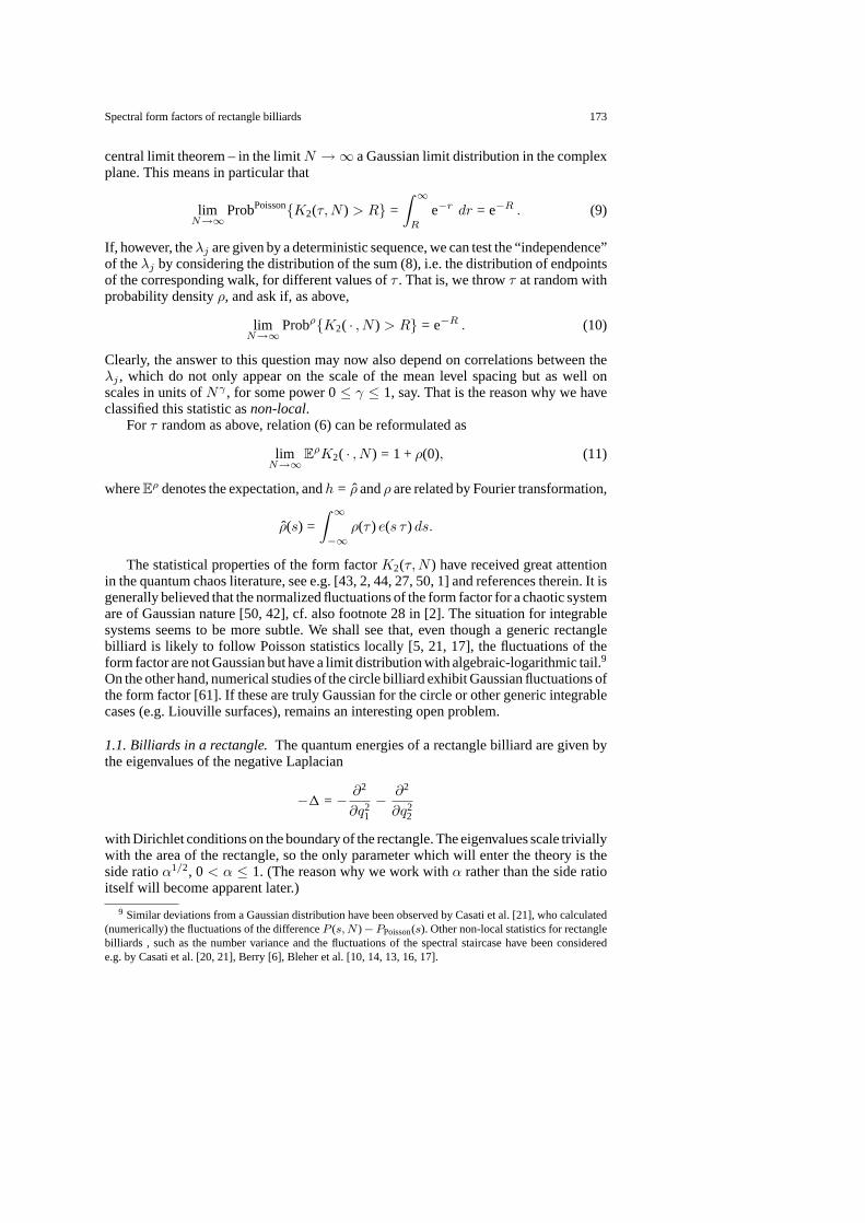
Fig. 1.A walk of N = 16 unit steps in the complex plane

In the present article, we shall study similarnon-localstatistical properties, whichare, however much closer linked to thelocal level spacing statistics. The central object ofour investigation will be thespectral form factorK2(τ,N ) (also calledpair correlationform factor), which is defined as the Fourier transform of the pair correlation density,

K2(τ,N ) =∫ ∞

−∞R2(s,N ) e(τ s) ds,

R2(s,N ) =∫ ∞

−∞K2(τ,N ) e(−s τ ) dτ

with e(z) ≡ e2πi z, hence,

K2(τ,N ) = |N−1/2N∑j=1

e(λj τ )|2. (7)

The sum

N∑j=1

e(λj τ ) (8)

may be viewed as a walk in the complex plane (Fig. 1), consisting ofN steps of unitlength, whose direction is determined by the phasesξj = 2πλjτ . In the case when theλj come from a Poisson process, the probability of finding the end point afterN stepsoutside a disk of radius

√NR (R is a fixed constant) has – by virtue of the classical

7 E.g. billiards in a rectangle and tori [34, 9, 10, 14, 13], Liouville surfaces [41, 15], other surfaces ofrevolution [11], and Zoll surfaces [57]. For a survey see [12].

8 In contrast, for chaotic systems the fluctuations of the spectral staircase are conjectured to be Gaussian[4, 3], based mainly on numerical evidence.


central limit theorem – in the limitN → ∞ a Gaussian limit distribution in the complexplane. This means in particular that

limN→∞

ProbPoisson{K2(τ,N ) > R} =∫ ∞

R

e−r dr = e−R . (9)

If, however, theλj are given by a deterministic sequence, we can test the “independence”of theλj by considering the distribution of the sum (8), i.e. the distribution of endpointsof the corresponding walk, for different values ofτ . That is, we throwτ at random withprobability densityρ, and ask if, as above,

limN→∞

Probρ{K2( · , N ) > R} = e−R . (10)

Clearly, the answer to this question may now also depend on correlations between theλj , which do not only appear on the scale of the mean level spacing but as well onscales in units ofNγ , for some power 0≤ γ ≤ 1, say. That is the reason why we haveclassified this statistic asnon-local.

For τ random as above, relation (6) can be reformulated as

limN→∞

EρK2( · , N ) = 1 +ρ(0), (11)

whereEρ denotes the expectation, andh = ρ andρ are related by Fourier transformation,

ρ(s) =∫ ∞

−∞ρ(τ ) e(s τ ) ds.

The statistical properties of the form factorK2(τ,N ) have received great attentionin the quantum chaos literature, see e.g. [43, 2, 44, 27, 50, 1] and references therein. It isgenerally believed that the normalized fluctuations of the form factor for a chaotic systemare of Gaussian nature [50, 42], cf. also footnote 28 in [2]. The situation for integrablesystems seems to be more subtle. We shall see that, even though a generic rectanglebilliard is likely to follow Poisson statistics locally [5, 21, 17], the fluctuations of theform factor are not Gaussian but have a limit distribution with algebraic-logarithmic tail.9

On the other hand, numerical studies of the circle billiard exhibit Gaussian fluctuations ofthe form factor [61]. If these are truly Gaussian for the circle or other generic integrablecases (e.g. Liouville surfaces), remains an interesting open problem.

1.1. Billiards in a rectangle.The quantum energies of a rectangle billiard are given bythe eigenvalues of the negative Laplacian

−1 = − ∂2

∂q21

− ∂2

∂q22

with Dirichlet conditions on the boundary of the rectangle. The eigenvalues scale triviallywith the area of the rectangle, so the only parameter which will enter the theory is theside ratioα1/2, 0< α ≤ 1. (The reason why we work withα rather than the side ratioitself will become apparent later.)

9 Similar deviations from a Gaussian distribution have been observed by Casati et al. [21], who calculated(numerically) the fluctuations of the differenceP (s, N ) − PPoisson(s). Other non-local statistics for rectanglebilliards , such as the number variance and the fluctuations of the spectral staircase have been considerede.g. by Casati et al. [20, 21], Berry [6], Bleher et al. [10, 14, 13, 16, 17].

174 J. Marklof

Taking the area to be 4π we have eigenvalues

E(α)m,n =

π

4(α1/2m2 + α−1/2n2), m, n ∈ N,

which we label in increasing order and with multiplicity by 0< λ(α)1 < λ(α)

2 ≤ λ(α)3 ≤

. . . . This sequence clearly satisfies (1), since the number of lattice points in an ellipseof areaλ is asymptoticallyλ. More precisely, we have

#{j : λ(α)j ≤ λ} = λ− π−1/2(α1/4 + α−1/4) λ1/2 +Oγ(λγ), (12)

where the relation is conjectured to hold for anyγ > 14; the best bound so far,γ > 23

73,is due to Huxley [36].

1.2. The main results.Let us viewτ as a random variable, which is distributed onthe compact intervalI ⊂ R with a piecewise continuous probability densityρ, andαas a random variable with piecewise continuous probability densityσ on the compactintervalA ⊂ R+ − {0}. The expectationEρ,σ for the random variablef (τ, α) is thendefined as

Eρ,σf =∫I

∫A

f (τ, α) ρ(τ ) σ(α) dτ dα,

and its probability to be greater thanR by

Probρ,σ{f > R} =∫I

∫A

DR(τ, α) ρ(τ ) σ(α) dτ dα,

with the distribution function

DR(τ, α) =

{1 if f (τ, α) > R

0 otherwise.

Theorem 1.1. There exists a decreasing function9 : R+ → R+ with

9(0) = 1,∫ ∞

09(R) dR = 1,

9(R) ∼ cR−2 logR (for R → ∞),

discontinuous only for at most countably manyR, such that,

limN→∞

Probρ,σ{K2( · , N ) > R} = 9(R),

except possibly at the discontinuities of9(R).

The constantc is given by the expression

c =2π6

∫R2

|∫t21+t22≤1

e(t21u1 + t22u2) d2t|4d2u. (13)


Remarks. (A)The condition∫∞

0 9(R) dR = 1 is consistent with a Gaussian limitdistribution and thus consistent with the fact that the pair correlation function is the onefor Poisson random numbers.

(B) The condition9(R) ∼ cR−2 logR implies that the limit distribution is non-Gaussian. In particular, the higher moments

∫∞0 Rkd9(R) (k > 2) diverge. This di-

vergence has the following origin. Just as the momentk = 1 is related to the paircorrelation functionR2(s,N ) (i.e. counting spacings), the momentk = 2 is related tothe density

1N2

N∑j1,j2,k1,k2=1

δ(s− λj1 − λj2 + λk1 + λk2), (14)

and thus to (with the above test functionh)

1N2

N∑j1,j2,k1,k2=1

h(λj1 + λj2 − λk1 − λk2), (15)

which amounts to counting the number of quadruples of eigenvalues such that

λj1 + λj2 − λk1 − λk2

is in the interval [−a, a], say. In the case of a rectangle billiard, this number grows like� (N logN )2, due to number-theoretic degeneracies: recall that in this case we countessentially the integersm1, . . . ,m4, n1, . . . , n4 ≤ √

N with

(m21 + αn2

1) + (m22 + αn2

2) − (m23 + αn2

3) − (m24 + αn2

4) (16)

in some interval. The number of solutions of

m21 +m2

2 = m23 +m2

4, n21 + n2

2 = n23 + n2

4

with m1, . . . ,m4, n1, . . . , n4 ≤ √N grows like� (N logN )2, due to Landau’s clas-

sical result on the number of ways of writing an integer as a sum of two squares.Hence the number of solutions of (16) in any arbitrarily small interval [−ε, ε] grows like� (N logN )2, hence the divergence of the second moment, at least for test functionsh with h(0) 6= 0. But sinceh is the Fourier transform of a probability density, we infact haveh(0) = 1. This explains the divergence of the momentsk = 2 and higher.Consequently, we cannot employ the method of moments to prove the above theorem.We shall instead use another approach based on the transformation formulas of thetafunctions, relating the existence of the limit distribution to the mixing property of certainflows, see Sect. 5 for details. This is essentially the same idea as in the proofs of thelimit theorems of theta sums

N∑n=1

e(n2x)

in [46, 47, 48], which is now generalized to theta sums with more variables. The methodspresented here could be further generalized to Siegel theta sums of arbitrary quadraticformsQ(ξ) of d variables, ∑

ξ∈Zd∩3N

e(Q(ξ) τ ).

176 J. Marklof

Here,3N denotes some suitable domain3 ⊂ Rd, which is magnified by a factor ofN .It would be interesting to see, in which cases the values of the above theta sums have alimit distribution forτ random. The expectation value of this limit distribution is relatedto the quantitative version of the Oppenheim conjecture forQ(ξ), cf. Eskin et al. [29, 30]and Borel’s survey [19].

(C) Theorem 1.1 implies that there cannot be a set ofα of non-zero Lebesgue measure,for which (for fixedα and randomτ ) Probρ{K2( · , N ) > R} converges to e−R. Weinstead have good reasons to believe the following to be true for thoseα, which arediophantine, i.e., badly approximable by rationals.10

Conjecture 1.2. Theorem 1.1 even holds whenα is not random but fixed, as long asαis diophantine. That means in particular

limN→∞

Probρ{K (α)2 ( · , N ) > R} = 9(R),

with the same function9(R) as before.

The truth of this conjecture is related to the equidistribution of horocycles in the prod-uct space0\ PSL(2,R) × 0\ PSL(2,R) (for details see Sect. 5, in particular Conjecture5.6, and Sect. 6).

The conjecture is obviously false for rationalα = pq . The following theorem follows

from the results in [39, 46], see Sect. 7 for details.

Theorem 1.3. Letψ be piecewise continuous and of compact support. Then there existsa decreasing function9( p

q ) : R+ → R+ with

9( pq )(0) = 1, 9( p

q )(R) ∼ c( pq ) R−1 (for R → ∞),

discontinuous for at most countably manyR, such that,

limλ→∞

Probρ{K ( pq )

2 ( · , λ) > R} = 9( pq )(R),

except possibly at the discontinuities of9( pq )(R).

In the special caseα = pq = 1 the constantc( p

q ) readsc(1) = 1/π.

Remark.The fact that now∫∞

0 9(R) dR = ∞ diverges is due to the well known de-generacy of values of rational quadratic forms at integers (cf. previous remark B). Inparticular, one has for the pair correlation function (Proposition 7.1)

EρK( p

q )2 ( · , N ) ∼ b( p

q ) logN (N → ∞). (17)

Forα = pq = 1 we haveb(1) = 1/π. The logarithmic divergence resembles the average

number of ways to write an integer as a sum of two squares, which is a classical result byLandau, cf. the previous Remark (B). As a consequence, the consecutive level spacingdistribution isP (s) = δ(s) for all rationalα. For more information on two-level statisticsfor the square billiard, cf. also Connors and Keating [24].

10 The precise definition of a diophantine number will be given later (Sect. 5). The set of diophantinenumbers is of full Lebesgue measure inR.


1.3. Basic definitions and notations.The expressionsx �a y andx = Oa(y) both meanthere exists a constantCa (which may depend on some additional parametera) suchthat |x| ≤ Ca|y|. The notationx = O(y−∞) is an abbreviation forx = OM (y−M ) foreveryM ≥ M0, for some suitably large constantM0. A piecewise continuousfunction isdiscontinuous only on a set of measure zero, and bounded on all compact sets. We denoteby S(Rn) the Schwartz class onRn, i.e. the space of smooth functionsf (t1, . . . , tn)which decrease rapidly whent21 + . . . + t2n → ∞. The same must hold for all derivativesof f .

2. Invariance Properties of the Form Factor

The pair correlation densityR2(s, λ) and the form factorK2(τ, λ) measure the statisticsof levels in an energy window [0, λ]. For technical reasons it is convenient to smooth thiswindow, i.e., choose a smooth cut-off functionψ ∈ C∞(R+), which is rapidly decreasingat∞ and consider the smoothed (inλ) pair correlation density

R2,ψ(s, λ) =1λ

∑λj ,λk

ψ(λjλ

) ψ(λkλ

) δ(s− λj + λk), (18)

and the smoothed form factor

K2,ψ(τ, λ) = |λ−1/2∑λj

ψ(λjλ

) e(λj τ )|2. (19)

In the case of the rectangle billiard the form factor has the explicit expression

K (α)2,ψ(τ, λ) = |λ−1/2

∑m,n∈N

ψ(π4 (α1/2m2 + α−1/2n2)

λ) ×

× e(π

4(α1/2m2 + α−1/2n2) τ )|2. (20)

For symmetry reasons, we can write the sum as

4∑m,n∈N

=∑m,n∈Z

−∑

m=0,n∈Z−

∑m∈Z,n=0

+∑

m=0,n=0

.

The form factor can now be expressed in terms of the theta functions

2f (z) = y1/4∑n∈Z

f (n y1/2) e(n2x), (21)

and

2f (z1; z2) = y1/41 y

1/42

∑m,n∈Z

f (my1/21 , n y

1/22 ) e(m2x1 + n2x2), (22)

wherezj = xj + i yj is a complex variable. Setting

f (t) = ψ(t2), f (t1, t2) = ψ(t21 + t22),

and

178 J. Marklof

z1 =π

4α1/2(τ + i λ−1), z2 =

π

4α−1/2(τ + i λ−1),

we have

K (α)2,ψ(τ, λ) =

116

|(π4

)−1/2 2f (z1, z2)

− λ−1/4[(π

4α1/2)−1/4 2f (z1) + (

π

4α−1/2)−1/4 2f (z2)

]+ λ−1/2ψ(0)|2. (23)

It is intuitively clear that in the limitλ → ∞ the most important contributions shouldcome from the two-variable theta sum. However, for special values ofα andτ this neednot be the case, but the set of exceptions is fortunately of measure zero. The followinglemma follows from standard estimates on theta sums [33].

Lemma 2.1. For almost allα andτ (with respect to Lebesgue measure) and anyε > 0we have

K (α)2,ψ(τ, λ) = K (α)

2,ψ(τ, λ) +Oα,τ,ε(λ−1/4+ε),

with

K (α)2,ψ(τ, λ) =

14π

|2f (z1, z2)|2.

The transformation formulas of theta functions (21) in one complex variable werethe starting point of the studies in [46, 47, 48], and can be readily generalized to thetwo-variable sum2f (z1; z2), by considering each variable separately.

Before stating the transformation formulas, we have to introduce some geometry.Every elementg in the Lie group PSL(2,R) = SL(2,R)/{±1} has a unique Iwasawadecomposition

g =

(1 x0 1

)(y1/2 0

0 y−1/2

)(cosφ − sinφsinφ cosφ

),

wherez = x + i y is a point in the upper half plane

H = {z = x + i y : x, y ∈ R, y > 0},andφ ∈ [0, π) parametrizes the circle S1, so the underlying manifold of PSL(2,R) maybe identified with the manifoldH × S1. The invariant volume element (Haar measure)reads in this choice of coordinates

dµ(g) =dx dy dφ

y2.

By virtue of the relation(a bc d

)(1 x0 1

)(y1/2 0

0 y−1/2

)(cosφ − sinφsinφ cosφ

)=

(1 x′0 1

)(y′1/2 0

0 y′−1/2

)(cosφ′ − sinφ′sinφ′ cosφ′

), (24)

where

x′ + i y′ =a(x + i y) + bc(x + i y) + d

, φ′ = φ + arg[c(x + i y) + d],


the action of PSL(2,R) onH × S1 is canonically given by

g (z, φ) =(gz, φ + arg(cz + d)

), g =

(a bc d

), (25)

whereg acts onz ∈ H by fractional linear transformations, i.e.,

g z =az + bcz + d

.

Thetheta group0θ, which is generated by the elements(1 10 1

)and

(0 −1/22 0

),

corresponding to the transformations(1 10 1

)(z, φ) =

(z + 1, φ),

(0 −1/22 0

)(z, φ) =

(− 14z, φ + argz),

is an example of a discrete subgroup of PSL(2,R), such that the quotient manifold

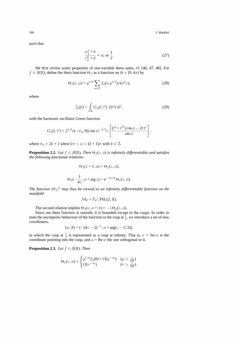
Mθ = 0θ\ PSL(2,R) = {0θh : h ∈ PSL(2,R)}has finite volumeµ(Mθ) = π2, but is not compact (with respect to the measure introducedabove). A fundamental region of0θ in H is (Fig. 2)

Fθ = {z ∈ H : |x| < 1/2, |z| > 1/2}. (26)

There are two cusps which are represented by the points at∞ and 12 (− 1

2 is equivalentto 1

2). It is well known that every rational point on the boundary Imz = 0 of H is0θ-equivalent to one of the cusp points, i.e. there is always an element(

a bc d

)∈ 0θ

y

-1/2 0 1/2x

Fig. 2. The fundamental regionFθ = {z ∈ H : |x| < 1/2, |z| > 1/2} in H for the theta group0θ . Thecusps are represented by the points at∞ and 1

2 . The thin lines indicate the symmetries of the surface

180 J. Marklof

such that

apq + b

cpq + d= ∞ or

12. (27)

We first review some properties of one-variable theta sums, cf. [46, 47, 48]. Forf ∈ S(R), define the theta function2f as a function onH × [0, 4π) by

2f (z, φ) = y1/4∑n∈Z

fφ(n y1/2) e(n2x), (28)

where

fφ(t) =∫

RGφ(t, t′) f (t′) dt′, (29)

with the harmonic oscillator Green function

Gφ(t, t′) = 21/2e(−σφ/8)| sinφ|−1/2e

[(t2 + t′2) cosφ− 2t t′

sinφ

],

whereσφ = 2k + 1 whenkπ < φ < (k + 1)π with k ∈ Z.

Proposition 2.2. Let f ∈ S(R). Then2f (z, φ) is infinitely differentiable and satisfiesthe following functional relations:

2f (z + 1, φ) = 2f (z, φ),

2f (− 14z, φ + argz) = e− iπ/4 2f (z, φ).

The function|2f |2 may thus be viewed as an infinitely differentiable function on themanifold

Mθ = 0θ\ PSL(2,R).

The second relation implies2f (z, φ + π) = − i 2f (z, φ).Since our theta function is smooth, it is bounded except in the cusps. In order to

state the asymptotic behaviour of the function in the cusp at12, we introduce a set of new

coordinates,

(w, θ) = (−(4z − 2)−1, φ + arg(z − 1/2)),

in which the cusp at12 is represented as a cusp at infinity. That is,v = Imw is thecoordinate pointing into the cusp, andu = Rew the one orthogonal to it.

Proposition 2.3. Letf ∈ S(R). Then

2f (z, φ) =

{y1/4fφ(0) +O(y−∞) (y > 1

100)O(v−∞) (v > 1

100).


The ranges for which the above relations hold, cover the entire fundamental region{z ∈ H : 0 < x < 1, |z| > 1/2, |z − 1| > 1/2}. (This new region is obtained fromthe old oneFθ by shifting the left half byx 7→ x+ 1.) Within these ranges, the relationsare uniform in (z, φ) (1st rel.), (w, θ) (2d rel.).

Forf ∈ S(R2), define the theta function2f as a function onH×[0, 4π)×H×[0, 4π)by

2f (z1, φ1; z2, φ2) = y1/41 y

1/42

∑m,n∈Z

fφ1,φ2(my1/21 , n y

1/22 ) e(m2x1 + n2x2), (30)

where

fφ1,φ2(t1, t2) =∫∫

R2

Gφ1(t1, t1′) Gφ2(t2, t2

′) f (t1′, t2′) dt1′dt2′, (31)

with the same harmonic oscillator Green functionGφ(t, t′) as before. It can be readilyverified thatfφ1,φ2(t1, t2) is again∈ S(R2) (use partial integration int1 andt2), so thesum defining2f is rapidly convergent for every (φ1, φ2).

Proposition 2.4. Letf ∈ S(R2). Then2f (z1, φ1; z2, φ2) is infinitely differentiable andsatisfies the following functional relations:

2f (z1 + 1, φ1; z2, φ2) = 2f (z1, φ1; z2, φ2),

2f (− 14z1

, φ1 + argz1; z2, φ2) = e− iπ/4 2f (z1, φ1; z2, φ2),

2f (z2, φ2; z1, φ1) = 2f (z1, φ1; z2, φ2).

The function|2f |2 may thus be viewed as an infinitely differentiable function on themanifold

M2θ = 0θ\ PSL(2,R) × 0θ\ PSL(2,R).

The second relation implies2f (z1, φ1 + π; z2, φ2) = − i 2f (z1, φ1; z2, φ2).As mentioned above, the proof of the proposition follows exactly the lines of the

analogous proposition for one-variable theta functions, compare e.g. [47].As a fundamental region of0θ × 0θ we choose the set

F = Fθ × [0, π) × Fθ × [0, π). (32)

The four cusps of codimension two are represented by

(∞, φ1; z2, φ2), (12, φ1; z2, φ2), (z1, φ1; ∞, φ2), (z1, φ1;

12, φ2);

every point of the form

(p

q, φ1; z2, φ2), (z1, φ1;

p

q, φ2),

p

q∈ Q

is equivalent to one of those four, compare (27).

182 J. Marklof

Proposition 2.5. Letf ∈ S(R2). Then

2f (z1, φ1; z2, φ2) =

=

(y1 y2)1/4fφ1,φ2(0, 0) +O((y1 y2)−∞) (y1 >

1100, y2 >

1100)

O((v1 v2)−∞) (v1 >1

100, v2 >1

100)

O(y1/41 v−∞

2 ) (y1 >1

100, v2 >1

100)

O(v−∞1 y

1/42 ) (v1 >

1100, y2 >

1100).

These relations are uniform in (z1, φ1; z2, φ2) (1st rel.), (w1, θ1;w2, θ2) (2d rel.),(z1, φ1;w2, θ2) (3d rel.), (w1, θ1; z2, φ2) (4th rel.). The proof follows directly from Propo-sition 2 in [46].

The inner products and norms of the L2 spaces in question are defined as usual by

(f, g)L2(R2) =∫∫

R2

f g d2x, ‖f‖L2(R2) =√

(f, f )L2(R2) (33)

and

(F,G)L2(M2θ

) =∫∫

M2θ

F G d2µ, ‖F‖L2(M2θ

) =√

(F, F )L2(M2θ

). (34)

By virtue of the last proposition, it is clear that|2f | is in L2(M2θ). If f is even,

i.e.f (t1, t2) = f (−t1, t2) = f (t1,−t2), we have the relation

12π2

‖2f‖L2(M2θ

) = ‖f‖L2(R2), (35)

compare [46], Proposition 4.

3. Regime I: |τ | � λ−1/2−ε

We begin with the regime where|τ | ≤ CIλ−γ with γ > 1

2, andCI an arbitrary constant.The behaviour of the form factor is entirely determined by the values of the theta functionin the cusp at∞, since

K (α)2,ψ(τ, λ) =

14π

|2f (z1, 0;z2, 0)|2 =1

4π|2f (− 1

4z1, argz1; − 1

4z2, argz2)|2

with

− 14z1

=1

πα1/2

−τ + i λ−1

τ2 + λ−2, argz1 = arg(τ + i λ−1),

− 14z2

=1

πα−1/2

−τ + i λ−1

τ2 + λ−2, argz2 = arg(τ + i λ−1).

Forλ → ∞, the imaginary part of−1/4zj becomes infinitely large, so Proposition 2.5is applicable, yielding

K (α)2,ψ(τ, λ) =

14π2

|farg(τ+i λ−1),arg(τ+i λ−1)(0, 0)|2 λ−1

τ2 + λ−2+O(λ−∞) (36)

which holds uniformly for|τ | ≤ CIλ−γ . It is easy to see that


|farg(τ+i λ−1),arg(τ+i λ−1)(0, 0)|2

= 4λ2(τ2 + λ−2) |∫∫

e[(t21 + t22)τλ] f (t1, t2) dt1dt2|2

= 4λ2(τ2 + λ−2) |π∫ ∞

0e(rτλ)ψ(r) dr|2. (37)

Therefore

K (α)2,ψ(τ, λ) = |

∫ ∞

0e(rτλ)ψ(r) dr|2 λ +O(λ−∞) (38)

for λ → ∞ uniformly in |τ | ≤ CIλ−γ . In this regime, the form factor looks therefore

asymptotically as a delta mass at zero: upon applying a test functionρ we have∫ CIλ−γ

−CIλ−γ

ρ(τ )K (α)2,ψ(τ, λ) dτ ∼

∫ CIλ1−γ

−CIλ1−γ

ρ(τ/λ)|∫ ∞

0e(rτ )ψ(r) dr|2dτ,

and withρ(τ/λ) ∼ ρ(0) for τ ∈ [−CIλ1−γ , CIλ1−γ ] the above reduces to

∼ ρ(0)∫ ∞

−∞|∫ ∞

0e(rτ )ψ(r) dr|2dτ = ρ(0)

∫ ∞

0ψ(r)2dr

by Parseval’s equality. In summary,∫ CIλ−γ

−CIλ−γ

ρ(τ )K (α)2,ψ(τ, λ) dτ ∼

∫ CIλ−γ

−CIλ−γ

ρ(τ )K (α)2,ψ(τ, λ) dτ

∼ ρ(0)∫ ∞

0ψ(r)2dr. (39)

Regime I is usually referred to as thesaturation regime, since the number variance62(L)saturates in this regime, in contrast to the prediction for a Poisson process [6, 16].

4. Regime II: λ−1/2−ε � |τ | � λ−1/2+ε

Regime II is defined as the region whereCIλ−1/2−ε ≤ |τ | ≤ CIIλ−1/2+ε, withCI and

CII arbitrary positive constants. From the discussion of Regime I it is clear that the formfactor in Regime II can at most grow like

K2,ψ(τ, λ) = Oε(λ2ε), (40)

which is obtained from (38) forτ = λ−1/2−ε. The otherτ -values in Regime II arebounded farther away from the cusp, so that the above indeed gives an upper bound.The most interesting part of Regime II is whenCIλ−1/2 ≤ |τ | ≤ CIIλ

−1/2. Let us putω = τλ1/2. Then we have for largeλ,

− 14zj

=1

πα±1/2

−ωλ−1/2 + i λ−1

ω2λ−1 + λ−2∼ 1πα±1/2

(−ω−1λ1/2 + i ω−2)

and

184 J. Marklof

argzj = arg(ωλ−1/2 + i λ−1) → 0+.

Since the series defining2f (z1, φ1; z2, φ2) converges uniformly fory1 andy2 in com-pacta, we finally obtain

K (α)2,ψ(τ, λ) ∼ K (α)

2,ψ(τ, λ) ∼ K(1/α)2,ψ (− 4

π2

λ1/2

ω,

4π2

1ω2

) (λ → ∞) (41)

uniformly for |ω| = |τ |λ1/2 ∈ [CI , CII ].Before turning to Regime III (τ ∼ const.), where we shall study the fluctuations of the

form factor around its mean, we will have to prove some facts about the equidistributionof certain sets inM2

θ.

5. Ergodicity, Mixing and Equidistribution

In this section we discuss some ergodic properties of the geodesic flow on hyperbolicsurfaces of finite area, whose unit tangent bundle is represented by the quotientM =0\ PSL(2,R), where0 is a discrete subgroup, such as the theta group0θ. The surfaceshould only have a finite number of cusps (≥ 0), and we assume that, if there is at leastone cusp, the half-plane coordinates are chosen in such a way that one of the cuspsappears as the standard cusp of unit width at∞.

Consider the following three flows onM = 0\ PSL(2,R), defined by right transla-tion,

g 7→ g8t, 8t =

(et/2 00 e−t/2

), (42)

and

g 7→ g9t±, 9t

+ =

(1 t0 1

), 9t

− =

(1 0t 1

). (43)

These flows actually represent the geodesic and the (positive and negative) horocy-cle flow on the unit tangent bundle of the surface0\H, which can be identified with0\ PSL(2,R) (the angleφ is in fact− 1

2 times the orientation angle of the tangent vector).These flows are well known to be ergodic and mixing [25]. The mixing property can bestated as follows.

Proposition 5.1. LetF,G ∈ L2(M). Then

limt→±∞

∫MF (g)G(g8t) dµ(g) =

1µ(M)

∫MF dµ

∫MG dµ.

The mixing property has an interesting consequence for the asymptotic distributionof long arcs of horocycles, which is stated in the following corollary. In fact, the in-vestigation of measures concentrated along unstable fibers (which in our case are thehorocycles) is a central issue in the theory of dynamical systems. Our proof will followan idea of Eskin and McMullen [28], Theorem 7.1.; for related methods, cf. Kleinbockand Margulis [40], Sect. 2.2.1. and references therein.


Corollary 5.2. LetF be bounded and piecewise continuous onM, andh be piecewisecontinuous and of compact support onR. Then, for anyg0 ∈ M,

limt→−∞

∫Rh(u)F (g09

u+8t) du =

1µ(M)

∫MF dµ

∫Rh du.

Proof. Every elementg =(a bc d

) ∈ SL(2,R) with d 6= 0 can be written as a product

g = ±9u+8a9b

−. (44)

Let F be continuous on PSL(2,R), left-invariant under0 and compactly supportedwhen viewed as a function onM = 0\ PSL(2,R). Let furthermoreH be the functionon PSL(2,R) defined for some fixedε > 0 by

H(g) =

{h(u) 1

εχ(aε )χ(b) for g = 9u+8a9b

−0 for g =

(a bc 0

),

whereχ is the characteristic function of the interval [− 12 ,

12]. Consider the integral∫

PSL(2,R)H(g)F (g0g8

t) dµ(g) =∫

PSL(2,R)H(9u

+8a9b−)F (g09

u+8a9b

−8t) dµ.(45)

The bi-invariant Haar measure in these coordinates is given by

dµ = e−a da db du. (46)

Step A.Now using the relation9b−8t = 8t9b et

− the integral transforms to∫PSL(2,R)

H(9u+8a9b

−)F (g09u+8a+t9b et

− ) dµ. (47)

The distance (with respect to the invariant metric on PSL(2,R)) between the pointsg09

u+8a+t9b et

− andg09u+8a+t is b et, hence

F (g09u+8a+t9b et

− ) = F (g09u+8a+t) +O(b et), (48)

where the implied constant does not depend onu,a, b or t, forF is uniformly continuous.For−t large we thus have∫

PSL(2,R)H(9u

+8a9b−)F (g09

u+8a+t9b et

− ) dµ

=∫

R2

h(u)1εχ(a

ε)F (g09

u+8a+t) e−a da du +O(et). (49)

Step B.We can rewrite (45) as∫PSL(2,R)

H(g−10 g)F (g8t) dµ(g) =

∫M

(∑γ∈0

H(g−10 γg)

)F (g8t) dµ(g) (50)

186 J. Marklof

sinceF anddµ are0-left-invariant. The latter, by the mixing property, has the limit(notice that the functionG(g) =

∑γ∈0H(g−1

0 γg) is 0-left-invariant)

1µ(M)

∫MF dµ

∫M

∑γ∈0

H(g−10 γg) dµ(g)

=1

µ(M)

∫MF dµ

∫PSL(2,R)

H dµ

=1

µ(M)

∫MF dµ

∫R2

h(u)1εχ(a

ε) e−a da du. (51)

Step C.Combining Steps A and B we conclude that

limt→−∞

∫R2

h(u)χ(a)F (g09u+8εa+t) e−εa da du

=1

µ(M)

∫MF dµ

∫R2

h(u)χ(a) e−εa da du. (52)

By the uniform continuity ofF , given anyδ > 0, we find anε > 0 such that∫R2

h(u)χ(a)F (g09u+8εa+t) e−εa da du− δ

<

∫R2

h(u)χ(a)F (g09u+8t) da du

<

∫R2

h(u)χ(a)F (g09u+8εa+t) e−εa da du + δ. (53)

Since the limitst → −∞ on the left and right hand side exist for every fixedε, anddiffer by 2δ, which can be made arbitrarily small, the limit

limt→−∞

∫Rh(u)F (g09

u+8t) du =

1µ(M)

∫MF dµ

∫Rh(u) du (54)

must exist as well. In order to relax the condition of compact support forF notice that theassertion trivially holds forF ≡ const. One can then again use the inclusion principleto relax both the compact support hypothesis and the continuity hypothesis.�

Remarks. (A)It is crucial that the limit ist → −∞. The limit t → +∞ diverges, sincein this case the support of the measure converges towards a single limit point on theboundary ofH.

(B) Forg0 = 1 the assertion of the corollary can be stated in the (z, φ)-coordinates as

limy→0

∫Rh(x)F (z, 0)dx =

1µ(M)

∫MF dµ

∫Rh dx. (55)

In the case when the average is taken over aclosedhorocycle andh ≡ 1, this wasproved by Sarnak [53]. Hejhal [35] extended the result toh of the above class, but stillfor closed horocycles and forF which are independent ofφ, i.e. functions on0\H. Hisproof involves estimates on Poincare series of weight zero.


The observation of the previous corollary shall now be extended from averages overtranslates of horocycles to averages over translates of more general curves, which aregiven by the equation (in suitable coordinates)y = ef (x), wheref is a bounded realfunction. The casef ≡ const corresponds to horocycles.

Corollary 5.3. LetF , h be as before, and letf : R → R be continuous on the supportof h. Then, for anyg0 ∈ M,

limt→−∞

∫Rh(u)F (g09

u+8t+f (u)) du =

1µ(M)

∫MF dµ

∫Rh du.

That is, forg0 = 1,

limy→0

∫Rh(x)F (x + i y ef (x), 0)dx =

1µ(M)

∫MF dµ

∫Rh dx.

Proof. Repeat the proof of the previous corollary with

H(g) =

{h(u) 1

εχ(a−f (u)ε )χ(b) for g = 9u

+8a9b−

0 for g =(a bc 0

),

which still has compact support, sincef is bounded on the support ofh. The only maindifference to the previous proof is in Step C where we have instead

1ε

∫R2

h(u)χ(a− f (u)

ε)F (g09

u+8a+t) da du

=∫

R2

h(u)χ(a)F (g09u+8εa+t+f (u)) da du, (56)

and the conclusion is the same as before, forf is bounded on the domain of integration.�

The next step is to define flows on the product space

M2 = 0\ PSL(2,R) × 0\ PSL(2,R)

by the diagonal action

0\ PSL(2,R) × 0\ PSL(2,R) → 0\ PSL(2,R) × 0\ PSL(2,R), (57)

(g1, g2) 7→ (g1, g2)8t := (g18t, g28

t)

and(g1, g2) 7→ (g1, g2)9t

± := (g19t±, g29

t±).

We shall still call these flowsgeodesicor horocyclic, respectively. Each one is the directproduct of two mixing dynamical systems, and thus mixing itself [25]:

Proposition 5.4. LetF,G ∈ L2(M2). Then

limt→±∞

∫M2

F (g1, g2)G((g1, g2)8t) d2µ(g1, g2) =1

µ(M2)

∫M2

F d2µ

∫M2

G d2µ.

188 J. Marklof

The analogue of Corollaries 5.2 and 5.5 is the following:

Corollary 5.5. Let F be bounded and piecewise continuous onM2, h be piecewisecontinuous and of compact support onR2, andf = (f1, f2) : R2 → R2 continuous onthe support ofh. Then, for any(g1, g2) ∈ M2,

limt→−∞

∫R2

h(u1, u2)F (g19u1+ 8t+f1(u1,u2), g29

u2+ 8t+f2(u1,u2)) d2u

=1

µ(M2)

∫M2

F d2µ

∫R2

h d2u.

The proof of Corollary 5.2 obviously generalizes to this case. For (g1, g2) = 1 wehave

limy→0

∫R2

h(x1, x2)F (x1 + i y ef1(x1,x2), 0;x2 + i y ef2(x1,x2), 0)d2x

=1

µ(M2)

∫M2

F d2µ

∫R2

h d2x. (58)

There are reasons to believe that the above equidistribution results do not only holdfor two-dimensional averages over (x1, x2), but even for averages over one-dimensionallines given byx2 = ηx1. In the case when the lattice group0 is a congruence subgroupof PSL(2,R) (such as the theta group0θ), it has to be assumed, however, thatη is badlyapproximable by rationals, i.e. ∣∣∣∣η − p

q

∣∣∣∣ ≥ C

qκ

for all rationals pq and someκ ≥ 2. Numbersη satisfying this condition are calleddiophantine. The reason for the necessity of this condition will become clearer in Sect. 7.

Conjecture 5.6. SupposeM = 0\ PSL(2,R) with 0 a congruence subgroup ofPSL(2,R). LetF be bounded and piecewise continuous onM2, h be piecewise contin-uous and of compact support onR. If η is diophantine, we have for ally1, y2 > 0,

limy→0

∫Rh(x)F (x + i y1y, 0;ηx + i y2y, 0)dx =

1µ(M2)

∫M2

F d2µ

∫Rh dx.

The above observations on the equidistribution of certain sets will now be applied tounderstand the value distribution of the form factor in the most subtle Regime III, wherethe order of magnitude ofτ is independent ofλ.

6. Regime III: τ ∼ const

6.1. The expectation value.The following proposition is the analogue of Sarnak’sProposition 2.1(A) on the weak convergence of the pair correlation function in the caseof a two-dimensional family of tori [54]. Here, the weak convergence is with respect toour one-dimensional family of rectangles, parametrized byα. (Recall the definition ofρ andσ in Sect. 1.2.)


Proposition 6.1. Letψ be piecewise continuous and of compact support. Assume fur-thermoreρ is continuous at0. Then

limλ→∞

Eρ,σK2,ψ( · , λ) =(1 +ρ(0)

) ∫ ∞

0ψ(r)2dr.

Proof. We have to estimate the integral∫∫|λ−1/2

∑m,n∈N

ψ(π4 (α1/2m2 + α−1/2n2)

λ) ×

× e(π

4(α1/2m2 + α−1/2n2) τ )|2ρ(τ ) σ(α) dτ dα. (59)

Let us first assume all functions involved are infinitely differentiable. For later purposesit is furthermore convenient to assume that the functionsρandσ are not necessarily prob-ability densities, i.e., have averages also different from one. This freedom will be neededwhen we approximate piecewise continuous probability densities from above/below bysmoothρ andσ. To be able to use the inclusion principle forψ, we have to replace (59)by the slightly more general expression

1λ

∫∫ ∑m1,n1,m2,n2∈N

ψ1(π4 (α1/2m2

1 + α−1/2n21)

λ) ψ2(

π4 (α1/2m2

2 + α−1/2n22)

λ) ×

× e(π

4(α1/2(m2

1 −m22) + α−1/2(n2

1 − n22)) τ

)ρ(τ ) σ(α) dτ dα. (60)

We get back to (59) by settingψ1 = ψ2 = ψ. In the sequel,ψ1 andψ2 are taken to beC∞ with compact support. Let us split the domain of integration overτ into the threeparts corresponding to Regime I, Regime II and Regime III, that is,∫ ∞

0=∫ CIλ

−1/2−ε

0+∫ CIIλ

−1/2+ε

CIλ−1/2−ε

+∫ ∞

CIIλ−1/2+ε

and similarly for the integral over the negative axis. The first integral is similar to theone calculated in Sect. 3 (whereψ1 = ψ2 = ψ), see (39), and we have for largeλ,∫ CIλ

−1/2−ε

−CIλ−1/2−ε

∼ ρ(0)∫ ∞

0ψ1(r)ψ2(r)dr

∫σ(α) dα. (61)

This result can be obtained most easily by replacing the modulus squared of the thetafunction,|2f (z1, φ1; z2, φ2)|2, by the product

2f1(z1, φ1; z2, φ2) 2f2(z1, φ1; z2, φ2), (62)

with fν(t1, t2) = ψν(t21 + t22). The function in (62) can still be viewed as a function onM2

θ, cf. Proposition 2.4.The second integral vanishes to leading order, due to the bound analogous to bound

(40) valid in Regime II (Sect. 4), so∫ −CIλ−1/2−ε

−CIIλ−1/2+ε

+∫ CIIλ

−1/2+ε

CIλ−1/2−ε

� λ2ε(CIIλ−1/2+ε − CIλ

−1/2−ε) � λ−1/2+3ε. (63)

190 J. Marklof

We are left with the third integral, where|τ | ≥ CIIλ−1/2+ε, which we split into two

parts, thediagonalpart

1λ

∫∫|τ |≥CIIλ

−1/2+ε

∑m,n∈N

ψ1(π4 (α1/2m2 + α−1/2n2)

λ) ×

× ψ2(π4 (α1/2m2 + α−1/2n2)

λ) ρ(τ ) σ(α) dτ dα, (64)

which clearly converges forλ → ∞ to the desired expression11

∫ ∞

0ψ1(r)ψ2(r) dr

∫ρ(τ ) dτ

∫σ(α) dα,

and theoff-diagonalpart,

1λ

∑(m1,n1)6=(m2,n2)∈N2

∫∫|τ |≥CIIλ

−1/2+ε×

× ψ1(π4 (α1/2m2

1 + α−1/2n21)

λ)ψ2(

π4 (α1/2m2

2 + α−1/2n22)

λ) ×

× e(π

4(α1/2(m2

1 −m22) + α−1/2(n2

1 − n22)) τ ) ρ(τ ) σ(α) dτ dα. (65)

Substitutingx1 = π4α

1/2τ , x2 = π4α

−1/2τ the last expression equals

1λ

∑(m1,n1)6=(m2,n2)∈N2

∫∫| 2

π

√x1x2|≥CIIλ

−1/2+ε×

× ψ1(π

4

√x1x2m2

1 +√

x2x1n2

1

λ)ψ2(

π

4

√x1x2m2

2 +√

x2x1n2

2

λ) ×

× e(x1(m21 −m2

2) + x2(n21 − n2

2)) h(x1, x2) dx1 dx2, (66)

whereh is related toρ, σ and the Jacobian of the substitution in the obvious way,

h(x1, x2) =4π

√x1

x2x−1

2 ρ(4π

√x1x2)σ(

x1

x2). (67)

Let us divide (66) into the sums∑(m1,n1)6=(m2,n2)∈N2

=∑

m1 6=m2,n1 6=n2∈N+

∑m1 6=m2,n1=n2∈N

+∑

m1=m2,n1 6=n2∈N.

Partial integration with respect tox1 andx2 shows the first sum diverges only logarith-mically inλ, and, after some manipulations, this part of (66) turns out to be bounded by(use partial integration inx1, x2, and then re-substitute the old variablesτ andα)

11 Notice that the sum overm, n converges to the corresponding Riemann integral.


� 1λ

∑m1 6=m2,n1 6=n2�

√λ

∫∫|τ |≥CIIλ

−1/2+ε

ρ(τ )σ(α) dτ dατ2 |m2

1 −m22| |n2

1 − n22|

� 1λ1−ε′

∫|τ |≥λ−1/2+ε

ρ(τ )τ2

dτ � λ−1/2−ε+ε′∫

|τ |≥1

ρ(τλ−1/2+ε)τ2

dτ

� λ−1/2−ε+ε′ (68)

for any ε′ > 0. The remaining two sums can be shown to be of non-leading order bysimilar means.

We have thus shown so far that forλ → ∞,

1λ

∑(m1,n1),(m2,n2)∈N2

∫ψ1(

π4 (α1/2m2

1 + α−1/2n21)

λ)ψ2(

π4 (α1/2m2

2 + α−1/2n22)

λ) ×

× ρ(π

4(α1/2(m2

1 −m22) + α−1/2(n2

1 − n22)))σ(α) dα

−→∫ψ1(r)ψ2(r) dr

(ρ(0) +

∫ρ(τ ) dτ

)∫σ(α) dα. (69)

Taking finite linear combinationsH(r1, r2) =∑ψj1(r1)ψj2(r2) of functions of the

above type, we have

1λ

∑(m1,n1),(m2,n2)∈N2

∫H(

π4 (α1/2m2

1 + α−1/2n21)

λ,π4 (α1/2m2

2 + α−1/2n22)

λ) ×

× ρ(π

4(α1/2(m2

1 −m22) + α−1/2(n2

1 − n22)))σ(α) dα

−→∫H(r, r) dr

(ρ(0) +

∫ρ(τ ) dτ

)∫σ(α) dα. (70)

Let us now see how the smoothness condition onψ can be relaxed to piecewisecontinuousψ with compact support. Following the lines of the proof of Theorem 3.2 in[51], ψ(r1)ψ(r2) can now be approximated from above/below by smooth test functionsH(r1, r2), which are admissible for the previous derivation and for which∫

|H(r, r) − ψ(r)2| dr < ε. (71)

By the inclusion principle the statement of the proposition holds thus for piecewisecontinuousψ. The result can be further extended to piecewise continuousρ andσ byapproximating both sides of the relation

limλ→∞

Eρ,σK2,ψ( · , λ) =(1 +ρ(0)

) ∫ ∞

0ψ(r)2dr

from above and below using smooth functionsρε andσε, which areε-close12 to ρ andσ, respectively. �

12 In the L1 sense but also in the sense that|ρ(0) − ρε(0)| < ε, which is where the continuity ofρ at 0 isrequired.

192 J. Marklof

6.2. The limit distribution – smooth cut-off functions.Let us first consider the simplercase whenψ is a smooth cut-off function. The results will later be extended to moregeneral cut-off functions. We denote byS(R+) the space of even functions inS(R),restricted to the positive half lineR+.

Theorem 6.2. Letψ ∈ S(R+). Then there exists a decreasing function9 : R+ → R+

with

9ψ(0) = 1,∫ ∞

09ψ(R) dR =

∫ ∞

0ψ(r)2dr,


limλ→∞

Probρ,σ{K2,ψ( · , λ) > R} = 9ψ(R),

except possibly at the discontinuities of9ψ(R).

Theorem 6.3. For R → ∞, we have the asymptotic relation

9ψ(R) = cψR−2 logR + dψR

−2 +Oψ(R−∞),

where

cψ =2π6

∫R2

|∫

R2

e(t21u1 + t22u2)ψ(t21 + t22) d2t|4d2u.

The constantdψ is given by a more complicated expression, see the proof of this theorem.

The proofs of these theorems will be given below. The following conjecture is adirect consequence of the equidistribution hypothesis of Conjecture 5.6, compare theproof of Theorem 6.2.

Conjecture 6.4. Theorem 6.2 even holds whenα is not random but fixed, as long asαis diophantine. That means in particular

limλ→∞

Probρ{K (α)2,ψ( · , λ) > R} = 9ψ(R),

with the same function9ψ(R) as before.

This conjecture does not hold whenα is rational or well approximable by rationals,as we shall see in the next section.

Proof of Theorem 6.2.Apply Corollary 5.5, i.e. relation (58), whereχD is taken to bethe characteristic function of the set

D = {(z1, φ1; z2, φ2) ∈ M2θ :

14π

|2f (z1, φ1; z2, φ2)|2 > R}.

The boundary ofD can only have positive measure for a countable number ofR, other-wise this would be a contradiction to the measurability of2f . HenceχD is piecewisecontinuous except for countably manyR. We chose the functionh(x1, x2) in a way that

h(x1, x2)χD(x1 + i y ef1(x1,x2), 0;x2 + i y ef2(x1,x2), 0)d2x

= DR(τ, α, λ) ρ(τ )σ(α) dτ dα, (72)

where


x1 =π

4α1/2τ, x2 =

π

4α−1/2τ,

y =π

4λ−1, f1(x1, x2) = log

√x1

x2, f2(x1, x2) = log

√x2

x1,

and

DR(τ, α, λ) =

{1 if K (α)

2,ψ(τ, λ) > R

0 otherwise.

Since the compact intervalA does not contain 0, the functionsf1 andf2 are boundedon the domain of integration. Hence, except for at most countably manyR,

limλ→∞

Probρ,σ{K2,ψ( · , λ) > R} = 9ψ(R). (73)

To obtain the same result forK2,ψ, recall that by virtue of (23) we can express thedifference betweenK2,ψ andK2,ψ as the sum

λ−1/4F1(z1, φ1; z2, φ2) + λ−1/2F2(z1, φ1; z2, φ2)

+ λ−3/4F3(z1, φ1; z2, φ2) + λ−1ψ(0)2,

where theFj are sums of products of theta functions and their modulus is thereforemajorized by functions onM2

θ; it is therefore clear that

limλ→∞

Probρ,σ{|K2,ψ( · , λ) − K2,ψ( · , λ)| > ε} = 0 (74)

for arbitrarily small (but fixed)ε > 0. Hence for any givenε > 0, we have

Probρ,σ{K2,ψ( · , λ) > R + ε}≤ Probρ,σ{K2,ψ( · , λ) > R}

≤ Probρ,σ{K2,ψ( · , λ) > R− ε}, (75)

for every large enoughλ. The limits9ψ(R+ε) and9ψ(R−ε) of the left- and right-handside exist except for countably manyR, ε. Since

{(z1, φ1; z2, φ2) ∈ M2θ :

14π

|2f (z1, φ1; z2, φ2)|2 = R}

has positive measure only for countably manyR, the difference9ψ(R− ε)−9ψ(R+ ε)can be made arbitrarily small for suitable smallε > 0, except for countably manyR.

Finally, the relation9ψ(0) = 1 holds by definition,13 and the integral of9ψ can becalculated as follows (notice thatµ(M2

θ) = π4):

13 It might happen that9ψ(ε) ≤ C < 1 for arbitrarily smallε, but since we allow9ψ(R) to be discontin-uous at countably manyR, it is most sensible to normalize9ψ(0) = 1.

194 J. Marklof∫ ∞

09ψ(R) dR

=1

µ(M2θ)

∫ ∞

0µ{(z1, φ1; z2, φ2) ∈ F :

14π

|2f (z1, φ1; z2, φ2)|2 > R} dR

=1

4π5

∫M2

θ

|2f |2 d2µ =1π

∫R2

|f (t1, t2)|2 d2t =∫ ∞

0ψ(r)2dr, (76)

by virtue of relation (35). �

Proof of Theorem 6.3.It follows from the proof of Theorem 6.2 that for all but countablymanyR (recall the definition of the fundamental regionF in (32))

9ψ(R) =1π4µ{(z1, φ1; z2, φ2) ∈ F :

14π

|2f (z1, φ1; z2, φ2)|2 > R}

=2π4µ{(z1, φ1; z2, φ2) ∈ F : y1 > y2 and

14π

|2f (z1, φ1; z2, φ2)|2 > R}. (77)

The asymptotics of9ψ(R) is clearly determined by the large values of the theta function2f (z1, φ1; z2, φ2) in the cusps. By Proposition 2.5 and the refined asymptotic relation

2f (z1, φ1; z2, φ2) = y1/41 2f (φ1; z2, φ2) +O(y−∞

1 ) (78)

with the theta function

2f (φ1; z2, φ2) = y1/42

∑n∈Z

fφ1,φ2(0, n y1/22 ) e(n2x2),

we thus have

9ψ(R) =2π4µ{(z1, φ1; z2, φ2) ∈ F : y1 > y2,

y1 > 10 and1

4πy

1/21 |2f (φ1; z2, φ2)|2 > R} +O(R−∞)

=2π4

∫ π

0

∫Fθ

∫ π

0min{ 1

y2,

110, (4πR)−2|2f (φ1; z2, φ2)|4}dφ1

dx2 dy2 dφ2

y22

+O(R−∞). (79)

Let us first discuss the integral over the range

1y2< (4πR)−2|2f (φ1; z2, φ2)|4, i.e. (4πR)2 < y2|2f (φ1; z2, φ2)|4,

which, for largeR, requiresy2 to be large as well. From the asymptotic relation

2f (φ1; z2, φ2) =

{y

1/42 fφ1,φ2(0, 0) +O(y−∞

2 ) (y2 >1

100)O(v−∞

2 ) (v2 >1

100),(80)

compare Proposition 2.5, it follows that the integral over the range in concern is boundedfrom above and below by the same integral over the rangesy2|fφ1,φ2(0, 0)|2 > 4πR ∓CMR

−M (for anyM > 2 and a suitable constantCM ) which now can be worked outto give, forR large enough,


2π4

∫ π

0

∫ π

0

∫ ∞

(4πR∓CMR−M )/|fφ1,φ2(0,0)|2

∫ 1

0min{ 1

y2,

110

}dx2 dy2 dφ2

y22

dφ1

=2π4

∫ π

0

∫ π

0

∫ ∞

(4πR∓CMR−M )/|fφ1,φ2(0,0)|2

∫ 1

0

dx2 dy2 dφ2

y32

dφ1

=1π4

(4πR)−2∫ π

0

∫ π

0|fφ1,φ2(0, 0)|4 dφ1 dφ2 +OM (R−M ). (81)

As to the remaining range (4πR)2 > y2|2f (φ1; z2, φ2)|4, the same reasoning asbefore permits to give the upper and lower bounds

2π4

∫ π

0

∫ π

0

∫Fθ((4πR±CMR−M )/|fφ1,φ2(0,0)|2)

×

× min{ 110, (4πR)−2|2f (φ1; z2, φ2)|4}dx2 dy2 dφ2

y22

dφ1 (82)

with the truncated fundamental region

Fθ(T ) = {z ∈ Fθ : y < T}.The above integral, restricted to the range1

10 < (4πR)−2|2f (φ1; z2, φ2)|4, equals

210π4

∫ π

0

∫ π

0

∫(∗)

dy2

y22

dφ2 dφ1 +O(R−∞) = O(R−∞), (83)

where the range (∗) of integration of the inner integral is

(4πR)2

10|fφ1,φ2(0, 0)|4 ≤ y2 ≤ 4πR|fφ1,φ2(0, 0)|2 .

In order to work out the integral over the range110 > (4πR)−2|2f (φ1; z2, φ2)|4 let us

define the truncated function

Hf (φ1; z2, φ2) =

{|2f (φ1; z2, φ2)|4 − y2|fφ1,φ2(0, 0)|4 for y2 > 1|2f (φ1; z2, φ2)|4 otherwise,

(84)

which is rapidly decreasing in all cusps. The integral over the range under considerationcan now be expressed as

18π6R2

∫ π

0

∫ π

0

∫Fθ

Hf (φ1; z2, φ2)dx2 dy2 dφ2

y22

dφ1

+1

8π6R2

∫ π

0

∫ π

0

∫ 4πR/|fφ1,φ2(0,0)|2

1y2|fφ1,φ2(0, 0)|4dy2

y22

dφ2 dφ1

+O(R−∞). (85)

The second integral yields

18π6R2

logR∫ π

0

∫ π

0|fφ1,φ2(0, 0)|4 dφ1 dφ2

+1

8π6R2

∫ π

0

∫ π

0|fφ1,φ2(0, 0)|4 log

(4π/|fφ1,φ2(0, 0)|2) dφ1 dφ2. (86)

196 J. Marklof

Collecting all leading-order terms in the above estimates, we obtain

9ψ(R) =1

8π6

{∫ π

0

∫ π

0|fφ1,φ2(0, 0)|4 dφ1 dφ2

}R−2 logR

+1

8π6

{∫ π

0

∫ π

0|fφ1,φ2(0, 0)|4 log

(4π/|fφ1,φ2(0, 0)|2) dφ1 dφ2

+∫ π

0

∫ π

0

∫Fθ

Hf (φ1; z2, φ2)dx2 dy2 dφ2

y22

dφ1

+12

∫ π

0

∫ π

0|fφ1,φ2(0, 0)|4 dφ1 dφ2

}R−2 +O(R−∞). (87)

The coefficientscψ anddψ are thus determined. By virtue of (31) we have, after somechange of variables,∫ π

0

∫ π

0|fφ1,φ2(0, 0)|4 dφ1 dφ2 = 24

∫R2

|∫

R2

e(t21u1 + t22u2) f (t1, t2) d2t|4d2u, (88)

which concludes the proof of Theorem 6.3. �

6.3. The limit distribution – general cut-off functions.We shall now assume only thatf(and thusψ) is piecewise continuous and of compact support.

Theorem 6.5. Letψ be piecewise continuous and of compact support. Then there existsa decreasing function9 : R+ → R+ with

9ψ(0) = 1,∫ ∞

09ψ(R) dR =

∫ ∞

0ψ(r)2dr,


limλ→∞

Probρ,σ{K2,ψ( · , λ) > R} = 9ψ(R),

except possibly at the discontinuities of9ψ(R).

Proof. The proof follows along the lines of the proof of Theorem 4 in [46]. For a givenε > 0 choose a functionψε ∈ C∞(R+) of compact support, such that∫ ∞

0|ψ(r) − ψε(r)|2 dr < ε. (89)

The crucial observation is that, forλ large enough, we have∫I

∫A

K (α)2,ψ−ψε

(τ, λ) dτ dα ≤ Cε, (90)

for some constantC independent ofλ andε. This fact is a consequence of Proposition6.1 and Condition (89).

Consider the set

Sεy = {τ ∈ I, α ∈ A : K (α)2,ψ−ψε

(τ, λ) < ε1/2}.


The integral over the complement of this set must satisfy

Cε >

∫∫(I×A)−Sε

y

K (α)2,ψ−ψε

(τ, λ) dτ dα ≥∫∫

(I×A)−Sεy

ε1/2 dτ dα,

hence

|Sεy| > |I| |A| − Cε1/2. (91)

Define the distribution function

DR,ψ(τ, α, λ) =

{1 if K (α)

2,ψ(τ, λ) > R

0 otherwise,(92)

and the probability

9ψ,y(R) =∫I

∫A

DR,ψ(τ, α, λ) ρ(τ ) σ(α) dτ dα. (93)

By virtue of (91) we have the inclusions

9ψε,y(R + ε1/2) − C ′ε1/2 ≤ 9ψ,y(R) ≤ 9ψε,y(R− ε1/2) +C ′ε1/2, (94)

whereC ′ does not depend onε, y, R. By Theorem 6.2, fory → 0, the left and righthand side have the limits

limy→0

9ψε,y(R± ε1/2) = 9ψε (R± ε1/2) (95)

except for countably manyR, ε. Some analysis shows (for details compare [46]) that foreveryδ > 0 there is anε > 0 such that

9ψε(R− ε1/2) − 9ψε

(R + ε1/2) < δ (96)

(except for countably manyR). Hence there is a function9ψ(R) such that

limy→0

9ψ,y(R) = 9ψ(R), (97)

which proves the claim. �

6.4. Random walks.

Proof of Theorem 1.1.The task is to show that the difference between

Probρ,σ{∣∣∣∣ 1√

N

N∑j=1

e(λ(α)j τ )

∣∣∣∣2 > R

}and

Probρ,σ{∣∣∣∣ 1√

N

∑λ(α)

j≤N

e(λ(α)j τ )

∣∣∣∣2 > R

}vanishes forN → ∞, since then Theorem 1.1 will follow from Theorem 6.5. Firstnotice that

198 J. Marklof

∣∣∣∣ 1√N

N∑j=1

e(λ(α)j τ ) − 1√

N

∑λ(α)

j≤N

e(λ(α)j τ )

∣∣∣∣2 =

∣∣∣∣ 1√N

∑j∈X (α)

N

e(λ(α)j τ )

∣∣∣∣2, (98)

whereX (α)N is the set ofj defined by

X (α)N = {j ≤ N : λ(α)

j > N} ∪ {j > N : λ(α)j ≤ N}.

From the asymptotic relation (12) it can be readily seen that the number of elements inX (α)N is bounded by

#X (α)N �

√N, (99)

where the implied constant does not depend onα ∈ A (A fixed). It is therefore clearfrom the calculation done to prove Proposition 6.1 that∫

I

∫A

∣∣∣∣ 1√N

∑j∈X (α)

N

e(λ(α)j τ )

∣∣∣∣2 dτ dα (100)

vanishes for largeN . Hence we can use the inclusion principle in the same fashion asin the proof of Theorem 6.5 (the vanishing of (100) is the analogue of relation (90)) toprove the existence of the limit9(R), which furthermore has to equal9(R) = 9χ(R),with χ the characteristic function of the interval [0, 1]. �

7. Rational α

The simplest case isα = 1, sincez1 = z2 and so the form factor is related to the thetafunction2f (z, φ; z, φ) by

K (1)2,ψ(τ, λ) =

14π

|2f (z, 0;z, 0)|2.

The functionF (z, φ) = |2f (z, φ; z, φ)|2 can now be viewed as a function on the manifoldMθ, which is embedded as a three-dimensional submanifold inM2

θ, and we can applythe theorems which were developed in the beginning of Sect. 5. This observation holdsin a similar way for all rationalα = p

q ; however, the corresponding embedded three-

manifold M pq

becomes densely distributed inM2θ when the sequence of rationalspq

approaches an irrational. Let us discuss this in more detail.For a given integerN we define the congruence subgroups00(N ) of SL(2,Z) by

00(N ) =

{(a bc d

)∈ SL(2,Z) : c ≡ 0 modN

}. (101)

With

ηN =

(N 00 1

)we find [58] that

00(N ) = η−1N SL(2,Z)ηN ∩ SL(2,Z). (102)


The index of these subgroups in SL(2,Z) is finite, more precisely [58],

[SL(2,Z) : 00(N )] = N∏p primep|N

(1 +p−1). (103)

Consider now the form factor for rationalα = pq ,

K( p

q )

2,ψ(τ, λ) =1

4π|2f (z1, 0;z2, 0)|2 =

14π

|2f (pz, 0;qz, 0)|2, (104)

withz =

z1

p=z2

q=

π

4√pq

(τ + i λ−1).

For γ = η−1p γηp with γ =

(a bc d

) ∈ 00(4) we have the functional relations

|2f (pγz, φ + arg(pc z + d); qz, φ)|2= |2f (γpz, φ + arg(c pz + d); qz, φ)|2 = |2f (pz, φ; qz, φ)|2, (105)

and similarly

|2f (pz, φ; qγz, φ + arg(qc z + d))|2 = |2f (pz, φ; qz, φ)|2 (106)

for γ = η−1q γηq with γ ∈ 00(4). Therefore the function

|2( pq )

f (z, φ)|2 = |2f (pz, φ; qz, φ)|2 (107)

is invariant under the group

0( pq ) = η−1

p 00(4)ηp ∩ η−1q 00(4)ηq,

which, by virtue of (102), contains the congruence group00(4pq) ⊂ 0( pq ); hence0( p

q )

is of finite index in SL(2,Z) andM pq

= 0( pq )\ SL(2,R) has finite volume.

Using the theory developed in [46, 48] and the equidistribution of horocycles (Corol-lary 5.2) we can now prove the analog statements of the previous sections, but now forrationalα.

7.1. The expectation value.

Proposition 7.1. Let ψ be piecewise continuous and of compact support. Then, forλ → ∞,

EρK( p

q )

2,ψ( · , λ) ∼ b( p

q )

ψ logλ

for some constantb( p

q )

ψ . In the casepq = 1 we have in particular

b(1)ψ =

1π

∫ ∞

0ψ(r)2 dr.

200 J. Marklof

Sketch of the proof.The function|2( pq )

f (z, φ)|2 onM pq

= 0( pq )\ SL(2,R) is not bounded

so Corollary 5.2 is not directly applicable. However, there is a way of resolving thisdifficulty using a regularization with Eisenstein series, see [46, 48] for details. Comparealternatively Jurkat and van Horne [39] for a different approach.�

7.2. The limit distribution.

Theorem 7.2. Letψ be piecewise continuous and of compact support. Then there exists

a decreasing function9( p

q )

ψ with 9( p

q )

ψ (0) = 1, discontinuous for at most countably manyR, such that,

limλ→∞

Probρ{K ( pq )

2,ψ( · , λ) > R} = 9( p

q )

ψ (R),

except possibly at the discontinuities of9( p

q )

ψ (R). For largeR,

9( p

q )

ψ (R) ∼ c( p

q )

ψ R−1,

with some constantc( p

q )

ψ , which in the special casepq = 1 reads

c(1)ψ =

1π

∫ ∞

0ψ(r)2 dr.

Sketch of the proof.Simply use Corollary 5.2, and proceed as in the proof of Theorems6.2 and 6.5. Compare also the corresponding theorems in [46, 47, 48] and Jurkat andvan Horne’s results [37, 38, 39]. �

Acknowledgements.I thank G. Casati, A. Eskin, M.R. Haggerty, D.A. Hejhal, J.P. Keating, R.E. Prange,Z. Rudnick, U. Smilansky, G. Tanner and S. Zelditch for helpful discussions. The research was carried out atthe Basic Research Institute in the Mathematical Sciences, Hewlett-Packard Laboratories, Bristol, and at theProgramme on Disordered Systems and Quantum Chaos, Isaac Newton Instiute, Cambridge. I would like tothank both Institutes for their hospitality.

References

1. Alt, H., Graf, H.-D., Guhr, T., Harney, H.L., Hofferbert, R., Rehfeld, H., Richter, A. and Schardt, P.:Correlation-hole method for the spectra of superconducting microwave billiards. Phys. Rev. E55, 6674–6683 (1997)

2. Argaman, N., Imry, Y. and Smilansky, U.: Semiclassical analysis of spectral correlations in mesoscopicsystems. Phys. Rev. B47, 4440–4457 (1993)

3. Aurich, R., Backer, A. and Steiner, F.: Mode fluctuations as fingerprints of chaotic and non-chaoticsystems. Int. J. Mod. Phys. B11, 805–849 (1997)

4. Aurich, R., Bolte, J. and Steiner, F.: Universal signatures of quantum chaos. Phys. Rev. Lett.73, 1356–1359 (1994)

5. Berry, M.V. and Tabor, M.: Level clustering in the regular spectrum. Proc. Roy. Soc. A356, 375–394(1977)

6. Berry, M.V.: Semiclassical theory of spectral rigidity. Proc. Roy. Soc. A400, 229–251 (1985)7. Bleher, P.M.: The energy level spacing for two harmonic oscillators with golden mean ratio of frequencies.

J. Statist. Phys.61, 869–876 (1990)8. Bleher, P.M.: The energy level spacing for two harmonic oscillators with generic ratio of frequencies. J.

Statist. Phys.63, 261–283 (1991)9. Bleher, P.M.: On the distribution of the number of lattice points inside a family of convex ovals. Duke

Math. J.67, 461–481 (1992)


10. Bleher, P.M.: Distribution of the error term in the Weyl asymptotics for the Laplace operator on atwo-dimensional torus and related lattice problems. Duke Math. J.70, 655–682 (1993)

11. Bleher, P.M.: Distribution of energy levels of a quantum free particle on a surface of revolution. DukeMath. J.74, 45–93 (1994)

12. Bleher, P.M.: Trace formula for quantum integrable systems. lattice point problem, and small divisors.In: D. Hejhal et al. (eds.),Emerging Applications of Number Theory. IMA Volumes in Mathematics andits Applications, Vol.109, New York: Springer, 1998, pp. 1–38

13. Bleher, P.M., Cheng, Z., Dyson, F.J. and Lebowitz, J.L.: Distribution of the error term for the numberof lattice points inside a shifted circle. Commun. Math. Phys.154, 433–469 (1993)

14. Bleher, P.M., Dyson, F.J. and Lebowitz, J.L.: Non-Gaussian energy level statistics for some integrablesystems. Phys. Rev. Lett.71, 3047–3050 (1993)

15. Bleher, P.M., Kosygin, D.V. and Sinai, Ya.G.: Distribution of energy levels of quantum free particle onthe Liouville surface and trace formulae. Commun. Math. Phys.170, 375–403 (1995)

16. Bleher, P.M. and Lebowitz, J.L.: Energy-level statistics of model quantum systems: Universality andscaling in a lattice-point problem. J. Statist. Phys.74, 167–217 (1994)

17. Bleher, P.M. and Lebowitz, J.L.: Variance of number of lattice points in random narrow elliptic strip.Ann. Inst. H. Poincare Probab. Statist.31, 27–58 (1995)

18. Bohigas, O., Giannoni, M.-J. and Schmit, C.: Characterization of chaotic quantum spectra and univer-sality of level fluctuation laws. Phys. Rev. Lett.52, 1–4 (1984)

19. Borel, A.: Values of indefinite quadratic forms at integral points and flows on spaces of lattices. Bull.Am. Math. Soc.32, 184–204 (1995)

20. Casati, G., Guarneri, I. and Valz-Gris, F.: Degree of randomness of the sequence of eigenvalues. Phys.Rev. A30, 1586–1588 (1984)

21. Casati, G., Chirikov, B.V. and Guarneri, I.: Energy-level statistics of integrable quantum systems. Phys.Rev. Lett.54, 1350–1353 (1985)

22. Colin de Verdiere, Y.: Quasi-modes sur les varietes Riemanniennes. Invent. Math.43, 15–52 (1977)23. Colin de Verdiere, Y.: Sur le spectre des operateurs elliptiquesa bicaracteristiques toutes periodique.

Comment. Math. Helvetici54, 508–522 (1979)24. Connors, R.D. and Keating, J.P.: Two-point spectral correlations for the square billiard. J. Phys. A30,

1817–1830 (1997)25. Cornfeld, I.P., Fomin, S.V. and Sinai, Ya.G.:Ergodic Theory. Berlin–Heidelberg–New York: Springer,

198226. Duistermaat, J.J. and Guillemin, V.W.: The spectrum of positive elliptic operators and periodic bichar-

acteristics. Invent. Math.29, 39–79 (1975)27. Eckhardt, B. and Main, J.: Semiclassical form factor of matrix element fluctuations. Phys. Rev. Lett.75,

2300–2303 (1995)28. Eskin, A. and McMullen, C.: Mixing, counting, and equidistribution in Lie groups. Duke Math. J.71,

181–209 (1993)29. Eskin, A., Margulis, G. and Mozes, S.: On a quantitative version of the Oppenheim conjecture. Electron.

Res. Announc. Am. Math. Soc.1, 124–130 (1995)30. Eskin, A., Margulis, G. and Mozes, S.: Upper bounds and asymptotics in a quantitative version of the

Oppenheim conjecture. Ann. Math., to appear31. Eskin, A., Margulis, G. and Mozes, S.: Eigenvalue spacings on square 2-tori. In preparation32. Greenman, C.: The generic spacing distribution of the two-dimensional harmonic oscillator. J. Phys. A

29, 4065–4081 (1996)33. Hardy, G.H. and Littlewood, J.E.: Some problems in diophantine approximation, II. Acta Math.37,

193–239 (1914)34. Heath-Brown, D.R.: The distribution and moments of the error term in the Dirichlet divisor problem.

Acta Arith. 60, 389–415 (1992)35. Hejhal, D.: On value distribution properties of automorphic functions along closed horocycles.XVIth

Rolf Nevanlinna Colloquium (Joensuu, 1995), Amsterdam: de Gruyter, 1996, pp. 39–5236. Huxley, M.N.: Exponential sums and lattice points, II. Proc. London Math. Soc.66, 279–301 (1993);

Corrigenda ibid.68, 264 (1994)37. Jurkat, W.B. and van Horne, J.W.: The proof of the central limit theorem for theta sums. Duke Math. J.

48, 873–885 (1981)38. Jurkat, W.B. and van Horne, J.W.: On the central limit theorem for theta series. Michigan Math. J.29,

65–77 (1982)

202 J. Marklof

39. Jurkat, W.B. and van Horne, J.W.: The uniform central limit theorem for theta sums. Duke Math. J.50,649–666 (1983)

40. Kleinbock, D.Y. and Margulis, G.A.: Bounded orbits of nonquasiunipotent flows on homogeneousspaces. In: L.A. Bunimovich et al. (eds.),Sinai’s Moscow Seminar on Dynamical SystemsAMS Transl.(2) 171, Providence, RI: Am. Math. Soc., 1996, pp. 141–172

41. Kosygin, D.V., Minasov, A.A. and Sinai, Ya.G.: Statistical properties of the spectra of Laplace–Beltramioperators on iouville surfaces. Russ. Math. Surv.48, 1–142 (1993)

42. Lebœuf, P. and Iacomelli, G.: Statistical properties of the time evolution of complex systems I. Preprint,Orsay 1997, cond-mat/970970

43. Leviandier, L., Lombardi, M., Jost, R. and Pique, R.: Fourier transform: A tool to measure statisticallevel properties in very complex spectra. Phys. Rev. Lett.56, 2449–2452 (1986)

44. Lombardi, M. and Seligman, T.H.: Universal and nonuniversal statistical properties of levels and inten-sities for chaotic Rydberg molecules. Phys. Rev. A47, 3571–3586 (1993)

45. Major, P.: Poisson law for the number of lattice points in a random strip with finite area. Probab. TheoryRelated Fields92, 423–464 (1992)

46. Marklof, I.: Limit theorems for theta sums. Duke Math. J., to appear47. Marklof, J.: Theta sums, Eisenstein series, and the semiclassical dynamics of a precessing spin. In: D.

Hejhal et al. (eds.),Emerging Applications of Number Theory, IMA Volumes in Mathematics and itsApplications, Vol.109, New York: Springer, 1998, pp. 405–450

48. Marklof, J.: Limit Theorems for Theta Sums with Applications in Quantum Mechanics. Dissertation,Universitat Ulm, 1997, Aachen: Shaker Verlag, 1997

49. Pandey, A., Bohigas, O. and Giannoni, M.-J.: Level repulsion in the spectrum of two-dimensionalharmonic oscillators. J. Phys. A22, 4083–4088 (1989)

50. Prange, R.E.: The spectral form factor is not self-averaging. Phys. Rev. Lett.78, 2280–2283 (1997)51. Rudnick, Z. and Sarnak, P.: Zeros of principalL-functions and random matrix theory Duke Math. J.81,

269–322. (1996)52. Rudnick, Z. and Sarnak, P.: The pair correlation function for fractional parts of polynomials. Commun.

Math. Phys.194, 61–70 (1998)53. Sarnak, P.: Asymptotic behavior of periodic orbits of the horocycle flow and Eisenstein series. Commun.

Pure Appl. Math.34, 719–739 (1981)54. Sarnak, P.: Values at integers of binary quadratic forms. In:Harmonic analysis and number theory,

Montreal, 1996, CMS Conf. Proc.21, Providence, RI: Am. Math. Soc., 1997 pp. 181-20355. Sarnak, P.: Quantum chaos, symmetry and zeta functions. Lecture I: Quantum chaos, Curr. Dev. Math.

84–101 (1997)56. Sarnak, P.: Quantum chaos, symmetry and zeta functions. Lecture II: Zeta functions, Curr. Dev. Math.

102–115 (1997)57. Schubert, R.: The trace formula and the distribution of eigenvalues of Schrodinger operators on manifolds

all of whose geodesics are closed. DESY-Report 95–090 (1995)58. Shimura, G.:Introduction to the Arithmetic Theory of Automorphic Functions. Princeton, NJ: Princeton

Univ. Press, 197159. Sinai, Ya.G.: Poisson distribution in a geometric problem: In:Dynamical systems and statistical me-

chanics, (Moscow, 1991), Adv. Soviet Math.3, Providence, RI: Am. Math. Soc., 1991, pp. 199–21460. Slater, N.B.: Gaps and steps for the sequencenθ mod 1. Proc. Cambridge Philos. Soc.63, 1115–1123

(1967)61. Tanner, G.: private communication62. Uribe, A. and Zelditch, S.: Spectral statistics on Zoll surfaces. Commun. Math. Phys.154, 313–346

(1993)63. VanderKam, J.M.: Values at integers of homogeneous polynomials. Duke Math. J., to appear64. VanderKam, J.M.: Pair correlation of four-dimensional flat tori. Preprint, Princeton University, 199765. Weinstein, A.: Asymptotics of eigenvalue clusters for the Laplacian plus a potential. Duke Math. J.44,

883–892 (1977)66. Zelditch, S.: Level spacings for quantum maps in genus zero. Peprint, Isaac Newton Institute, Cambridge

1997

Communicated by Ya. G. Sinai

Spectral Form Factors of Rectangle Billiardsmajm/bib/spectral.pdf · Spectral form factors of...

Documents

Transcript of Spectral Form Factors of Rectangle Billiardsmajm/bib/spectral.pdf · Spectral form factors of...