Spectral Clustering

Jeyanthi S N

CptS 580 Topics in Machine Learning

Seminar Series

Nov 1,2011

  

Outline

Coverage Reference Linear Algebra + spectral theory Problems with spectral methods Kernel functions The paper Remnants

  

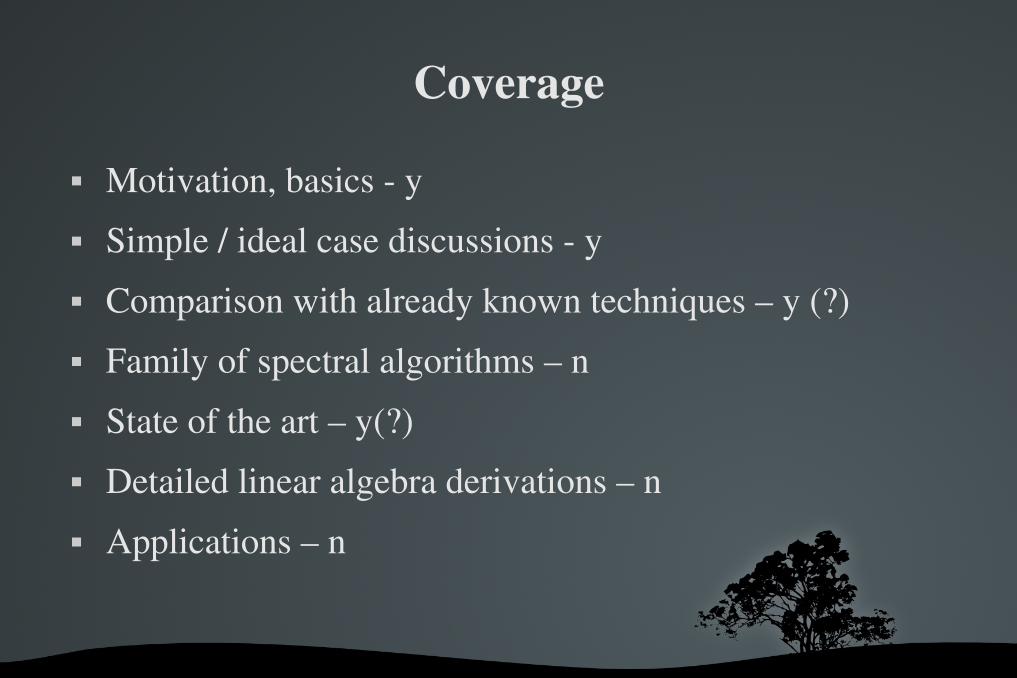
Coverage

Motivation, basics ­ y Simple / ideal case discussions ­ y Comparison with already known techniques – y (?) Family of spectral algorithms – n State of the art – y(?) Detailed linear algebra derivations – n Applications – n

  

Reference

A tutorial on spectral clustering

Statistics and Computing, Vol. 17, No. 4. (1 December 2007), pp. 395-416

  

Laplacian ( for K4)

0 1 1 1 1 0 1 1 1 1 0 1 1 1 1 0

3 0 0 0 0 3 0 0 0 0 3 0 0 0 0 3

3 -1 -1 -1 -1 3 -1 -1 -1 -1 3 -1 -1 -1 -1 3

4.4409e-16 0 0 0 0 4.00e+00 0 0 0 0 4.00e+00 0 0 0 0 4.00e+00

-0.5 -0.129633 0.734439 -0.440221 -0.5 -0.613036 -0.574510 -0.210061 -0.5 0.778522 -0.322605 -0.199572 -0.5 -0.035854 0.162676 0.849854

λ1=0, λ

2= 4, λ

3= 4, λ

4 = 4

W = Adj

D

L = D-W

Eigen vectors

diag(λ)

  

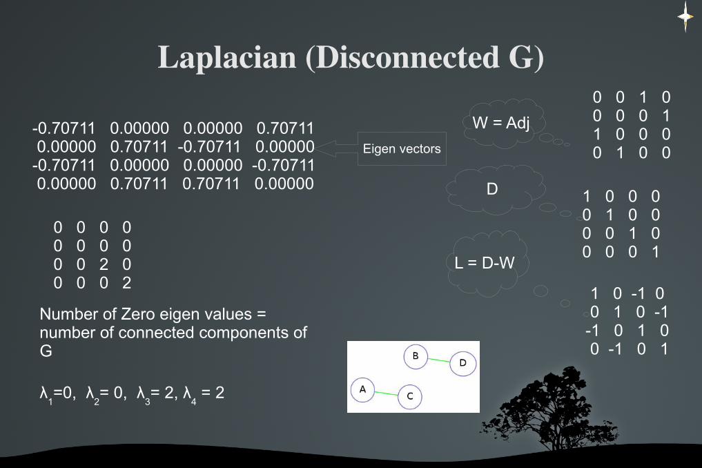
Laplacian (Disconnected G) 0 0 1 0 0 0 0 1 1 0 0 0 0 1 0 0

1 0 0 0 0 1 0 0 0 0 1 0 0 0 0 1

1 0 -1 0 0 1 0 -1 -1 0 1 0 0 -1 0 1

-0.70711 0.00000 0.00000 0.70711 0.00000 0.70711 -0.70711 0.00000 -0.70711 0.00000 0.00000 -0.70711 0.00000 0.70711 0.70711 0.00000

0 0 0 0 0 0 0 0 0 0 2 0 0 0 0 2

Number of Zero eigen values = number of connected components of G

λ1=0, λ

2= 0, λ

3= 2, λ

4 = 2

W = Adj

D

L = D-W

Eigen vectors

  

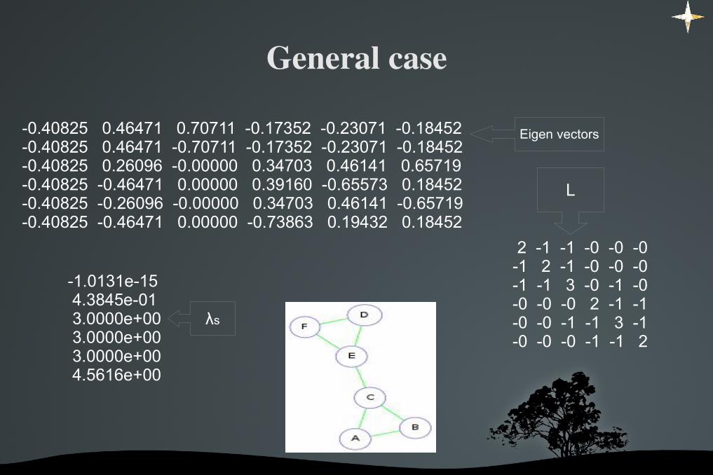
General case

2 -1 -1 -0 -0 -0 -1 2 -1 -0 -0 -0 -1 -1 3 -0 -1 -0 -0 -0 -0 2 -1 -1 -0 -0 -1 -1 3 -1 -0 -0 -0 -1 -1 2

-0.40825 0.46471 0.70711 -0.17352 -0.23071 -0.18452 -0.40825 0.46471 -0.70711 -0.17352 -0.23071 -0.18452 -0.40825 0.26096 -0.00000 0.34703 0.46141 0.65719 -0.40825 -0.46471 0.00000 0.39160 -0.65573 0.18452 -0.40825 -0.26096 -0.00000 0.34703 0.46141 -0.65719 -0.40825 -0.46471 0.00000 -0.73863 0.19432 0.18452

-1.0131e-15 4.3845e-01 3.0000e+00 3.0000e+00 3.0000e+00 4.5616e+00

L

λs

Eigen vectors

Matt

hia

sH

ein

and

Ulrik

evo

nLuxb

urg

:Short

Intr

oduct

ion

toSpec

tralClu

ster

ing

August

2007

13

Spectral clustering - main algorithms

Input: Similarity matrix S , number k of clusters to construct

• Build similarity graph

• Compute the first k eigenvectors v1, . . . , vk of the matrix{L for unnormalized spectral clustering

Lrw for normalized spectral clustering

• Build the matrix V ∈ Rn×k with the eigenvectors as columns

• Interpret the rows of V as new data points Zi ∈ Rk

v1 v2 v3

Z1 v11 v12 v13...

......

...Zn vn1 vn2 vn3

• Cluster the points Zi with the k-means algorithm in Rk .

  

Normalized laplacians

Commonly used laplacians Satisfy all the required properties

As many laplacians as there are authors

L sym :=D−1/2 LD−1 /2=I−D−1/2WD−1 /2

L rw :=D−1 L= I−D−1W

Matt

hia

sH

ein

and

Ulrik

evo

nLuxb

urg

:Short

Intr

oduct

ion

toSpec

tralClu

ster

ing

August

2007

7

Clustering using graph cuts

Clustering: within-similarity high, between similarity lowminimize cut(A, B) :=

∑i∈A,j∈B wij

Balanced cuts:RatioCut(A, B) := cut(A, B)( 1

|A| + 1|B|)

Ncut(A, B) := cut(A, B)( 1vol(A)

+ 1vol(B)

)

Mincut can be solved efficiently, but RatioCut or Ncut is NP hard.Spectral clustering: relaxation of RatioCut or Ncut, respectively.

Matt

hia

sH

ein

and

Ulrik

evo

nLuxb

urg

:Short

Intr

oduct

ion

toSpec

tralClu

ster

ing

August

2007

11

Solving Balanced Cut Problems

Relaxation for simple balanced cuts:

minA,B cut(A, B) s.t. |A| = |B|

Choose f = (f1, ..., fn)′ with fi =

{1 if Xi ∈ A

−1 if Xi ∈ B

• cut(A, B) =∑

i∈A,j∈B wij = 14

∑i ,j wij(fi − fj)

2 = 14f ′Lf

• |A| = |B| =⇒∑

i fi = 0 =⇒ f t1 = 0 =⇒ f ⊥ 1

• ‖f ‖ =√

n ∼ const.

minf f ′Lf s.t. f ⊥ 1, fi = ±1, ‖f ‖ =√

n

Relaxation: allow fi ∈ R

By Rayleigh: solution f is the second eigenvector of LReconstructing solution: Xi ∈ A ⇐⇒ fi >= 0, Xi ∈ B otherwise

  

K­way Graph Cut Objective functions

Ratiocut(A1, …, A

k):=

Ncut(A1, …, A

k):=

12∑i=1

i=k

(W (Ai , Ai)

∣Ai∣)=∑

i=1

i=k

(cut(Ai , Ai)

∣Ai∣)

12∑i=1

i=k

(W (Ai , Ai)

vol (Ai))=∑

i=1

i=k

(cut(Ai , Ai)

vol (Ai))

A⊂V , A=V ∖ A ,complement of A ,

∣A∣:=the number of vertices∈A

vol (A):=∑i∈A

d i

d i :=∑j=1

j=n

wij

W (A , B) := ∑i∈A , j∈B

wij

  

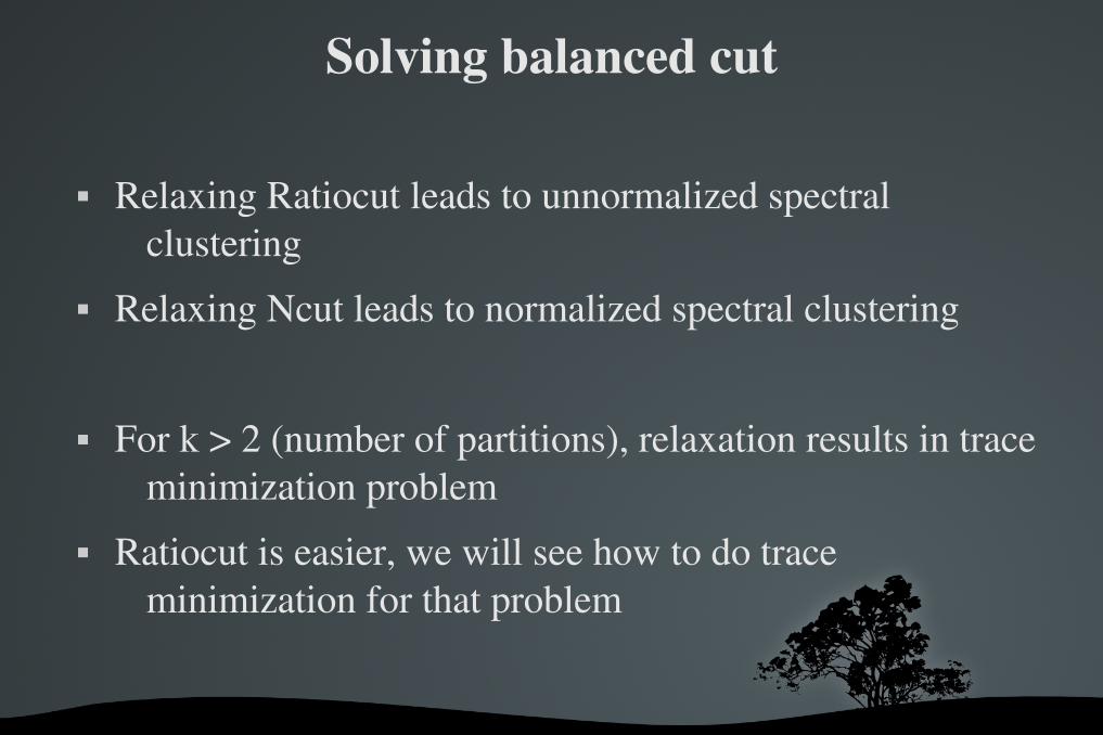
Solving balanced cut

Relaxing Ratiocut leads to unnormalized spectral clustering

Relaxing Ncut leads to normalized spectral clustering

For k > 2 (number of partitions), relaxation results in trace minimization problem

Ratiocut is easier, we will see how to do trace minimization for that problem

  

Ratio cut – Trace minimization

A1∪A2…∪Ak=V , Ai∩A j=∅ , Ai≠∅

Define k indicator vectors h j=(h1, j ,…hn , j) ' ,

hi , j= 1 /√∣A j∣if vi∈A j ,0 otherwise

(i=1,… , n ; j=1,… , k )

H∈ ℝn x k , H=[h1 ,… , hk ] , H ' H= I

hi ' Lhi=cut (Ai , Ai)

∣Ai∣

hi ' Lh i=(H ' LH )ii

  

Trace minimization

Ratiocut (A1 ,… , Ak)=∑i=1

k

(H ' LH )ii=Tr (H ' LH )

Problemof minimizing Ratiocut : minH ∈ℝ

n x k

Tr (H ' LH ) s.t H ' H= I

Use Rayleigh-Ritz procedure

  

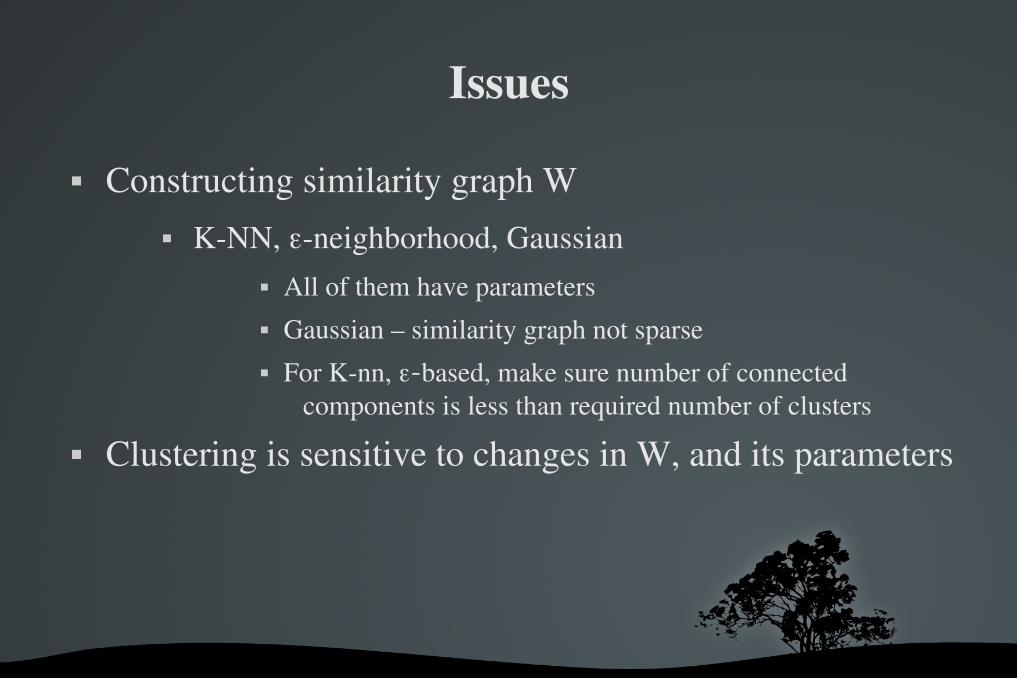
Issues

Constructing similarity graph W K­NN, ε­neighborhood, Gaussian

All of them have parameters Gaussian – similarity graph not sparse For K­nn, ε-based, make sure number of connected 

components is less than required number of clusters

Clustering is sensitive to changes in W, and its parameters

  

Different similarity Graphs

Datasets of different densities

* two half moons * One Gaussian cloud

  

Issues (2)

Computing Eigen vectors Number of clusters Laplacian

Regular graph : all three similar

Degree distribution has long tails, then better to use Lrw

Etc (some to follow in state of the art)

  

Kernel functions – a glance

x(1)

x(2)

Let the equation of the decision boundary of these two class points be

w1 x2(1)+√2w2 x (1) x (2)+w3 x

2(2)=0

x=(x (1)x (2)) z=(z (1)z (2)z (3)) ϕ :ℝ2

→ℝ3

Quadratic discriminant

  

Kernel functions (2)

ϕ( x) = ϕ(x (1)x (2)) = (z (1)=x2(1)z (2)=√2 x (1) x (2)z (3)=x2(2) ) = z

ϕ−space decision boundary : w1 z1+w2 z2+w3 z3 = 0

Linear discriminant in z-space

  

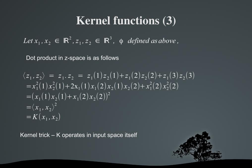
Kernel functions (3)

Dot product in z-space is as follows

Let x1 , x2 ∈ ℝ2 , z1 , z2 ∈ ℝ3 , ϕ defined asabove ,

⟨ z1 , z2⟩ = z1 . z2 = z1(1) z2(1)+z1(2) z2(2)+z1(3) z2(3)

=x12(1) x2

2(1)+2x1(1) x1(2) x2(1) x2(2)+x1

2(2) x2

2(2)

=( x1(1) x2(1)+x1(2) x2(2))2

=⟨ x1 , x2⟩2

=K ( x1 , x2)

Kernel trick – K operates in input space itself

  

A word about Mercer

This decade old theorem tells us that any ‘reasonable’ kernel function corresponds to some feature space.

A mercer kernel matrix is always positive semi definite Most useful property for constructing kernels Eg: gram matrix (also an affinity matrix) is a kernel matrix

Any PSD matrix can be regarded as a kernel matrix, that is an inner product matrix in some space – Nello Cristianini

  

Paper

Include weights and kernels in the objective function of   k­means

D ({π j} j=1k ) = ∑

j=1

k

∑a∈π j

w (a)∥ϕ(a)−m j∥2

where

m j=

∑b∈π j

w(b)ϕ(b)

∑b∈π j

w(b), π j :=clusters ,w (a):=weight for each point ' a '

  

Paper (2) Rewrite in trace maximization form using linear algebra 

tricks

m j=Φ j

W j e

s j

, where Φ=[ϕ(a1) ,… ,ϕ(an) ] , W j :=diag (w∈π j) ,

s j=∑a∈π j

w(a) , trace(AAT)=trace (AT A)=∥A∥F

2

  

Paper  (3)

Graph partitioning objectives naturally lead to trace maximization

Link the two trace maximizations with appropriate substitution

  

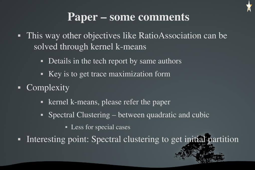
Paper – some comments This way other objectives like RatioAssociation can be 

solved through kernel k­means  Details in the tech report by same authors Key is to get trace maximization form

Complexity kernel k­means, please refer the paper Spectral Clustering – between quadratic and cubic

Less for special cases

Interesting point: Spectral clustering to get initial partition

  

State of the art

Original form is not scalable:  Parallel Spectral Clustering, Yangqiu Song, Chih­Jen Lin, Machine Learning and Knowledge 

Discovery in Databases (2008), pp. 374­389

Fast approxiate Spectral Clustering: Donghui Yan et al, SIGKDD 2009

Map­Reduce for Machine Learning on Multicore  Out of sample extension:

Spectral Embedded Clustering: A Framework for In­Sample and Out­of­Sample Spectral Clustering, Feiping Nie, Ivor W. Tsang, IJCAI'09 

Argues that in very high dimensional space spectral clustering fails (manifold assumption fail to hold)

Out­of­Sample Extensions for LLE, Isomap, MDS, Eigenmaps, and Spectral Clustering, Yoshua Bengio et al, NIPS (2004)

  

State of the art (2)

Can the two techniques (K­means, Spec clustering) be combined to form more efficient approach

Integrated KL (K­means – Laplacian) Clustering: A New Clustering Approach by Combining Attribute Data and Pairwise Relations, Fei Wang, Chris Ding, and Tao Li, SIAM 2009

Outlier handling (?)

Hard / soft clustering (?)

  

Other clustering algorithms

Partitioning Hierarchical  Density based Spectral clustering is all of the three above 

Top down clustering

Can capture arbitrary shaped points

Mutually k­nn, ε­neighborhood are density based similarity graph constructions

  

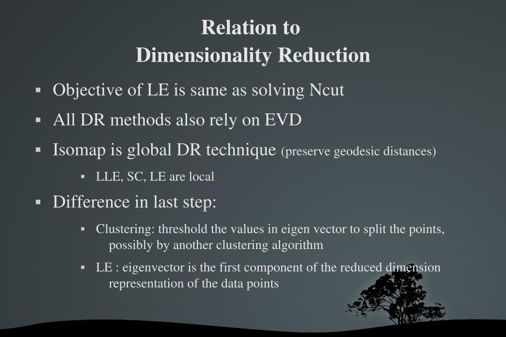
Relation to Dimensionality Reduction

Objective of LE is same as solving Ncut All DR methods also rely on EVD Isomap is global DR technique (preserve geodesic distances)

LLE, SC, LE are local 

Difference in last step:  Clustering: threshold the values in eigen vector to split the points, 

possibly by another clustering algorithm LE : eigenvector is the first component of the reduced dimension 

representation of the data points

  

Kernel Based Clustering

Mercer kernel­based clustering in feature space, M. Girolami, IEEE Trans. Neural Netw., vol. 13, no. 4, pp. 669–688, Apr. 2002 ­ uses EVD of affinity matrix

Clustering via kernel decomposition, A. Szymkowiak­Have, M. Girolami, and J. Larsen IEEE Trans. Neural Netw., Jan. 2006. 

Adapts from Kernel PCA, decomposition of gram matrix, non­parametric density estimation

Claims to provide accurate clustering, estimate model complexity, all parameters, probabilistic outcome for each point assignment, equivalence to SC

  

Discussion questions

Is Euclidean distance a generic distance? Effect of nature of attributes (discrete or continuous) on a 

clustering algorithm

  

References A Unified View of Kernel k­means, Spectral Clustering and Graph Partitioning, Inderjit Dhillon, Yuqiang 

Guan, Brian Kulis, Technical Report TR­04­25, 2005

www.stanford.edu/~boyd/ee263/lectures/symm.pdf

www.cs.yale.edu/homes/spielman/561/lect02­09.pdf

people.inf.ethz.ch/arbenz/ewp/Lnotes/lsevp.pdf

http://web.eecs.utk.edu/~dongarra/etemplates/node80.html#6462

http://www.svms.org/kernels/

Introduction to SVMs (and other kernel based learning methods), N.Cristianini, J.S.Taylor

Christopher J. C. Burges: Dimension Reduction: A Guided Tour. Foundations and Trends in Machine Learning 2(4): (2010)

Matt

hia

sH

ein

and

Ulrik

evo

nLuxb

urg

:Short

Intr

oduct

ion

toSpec

tralClu

ster

ing

August

2007

22

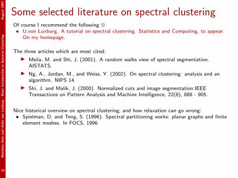
Some selected literature on spectral clusteringOf course I recommend the following ,• U.von Luxburg. A tutorial on spectral clustering. Statistics and Computing, to appear.

On my homepage.

The three articles which are most cited:

I Meila, M. and Shi, J. (2001). A random walks view of spectral segmentation.AISTATS.

I Ng, A., Jordan, M., and Weiss, Y. (2002). On spectral clustering: analysis and analgorithm. NIPS 14.

I Shi, J. and Malik, J. (2000). Normalized cuts and image segmentation.IEEETransactions on Pattern Analysis and Machine Intelligence, 22(8), 888 - 905.

Nice historical overview on spectral clustering; and how relaxation can go wrong:• Spielman, D. and Teng, S. (1996). Spectral partitioning works: planar graphs and finite

element meshes. In FOCS, 1996

  

Courtesy: www.gocomics.com/