Spectral clustering and the high-dimensional stochastic ... · PDF fileCLUSTERING FOR THE...
39
arXiv:1007.1684v3 [stat.ML] 13 Dec 2011 The Annals of Statistics 2011, Vol. 39, No. 4, 1878–1915 DOI: 10.1214/11-AOS887 c Institute of Mathematical Statistics, 2011 SPECTRAL CLUSTERING AND THE HIGH-DIMENSIONAL STOCHASTIC BLOCKMODEL 1 By Karl Rohe, Sourav Chatterjee and Bin Yu University of California, Berkeley Networks or graphs can easily represent a diverse set of data sources that are characterized by interacting units or actors. Social networks, representing people who communicate with each other, are one example. Communities or clusters of highly connected actors form an essential feature in the structure of several empirical networks. Spectral clustering is a popular and computationally feasible method to discover these communities. The stochastic blockmodel [Social Networks 5 (1983) 109–137] is a social network model with well-defined communities; each node is a member of one community. For a network generated from the Stochastic Blockmodel, we bound the number of nodes “misclus- tered” by spectral clustering. The asymptotic results in this paper are the first clustering results that allow the number of clusters in the model to grow with the number of nodes, hence the name high- dimensional. In order to study spectral clustering under the stochastic block- model, we first show that under the more general latent space model, the eigenvectors of the normalized graph Laplacian asymptotically converge to the eigenvectors of a “population” normalized graph Laplacian. Aside from the implication for spectral clustering, this provides insight into a graph visualization technique. Our method of studying the eigenvectors of random matrices is original. 1. Introduction. Researchers in many fields and businesses in several industries have exploited the recent advances in information technology to produce an explosion of data on complex systems. Several of the com- plex systems have interacting units or actors that networks or graphs can Received July 2010; revised December 2010. 1 Supported by Army Research Office Grant ARO-W911NF-11-1-0114; an NSF VIGRE Graduate Fellowship; NSF Grants CCF-0939370, DMS-07-07054, DMS-09-07632 and SES- 0835531 (CDI); and a Sloan Research Fellowship. AMS 2000 subject classifications. Primary 62H30, 62H25; secondary 60B20. Key words and phrases. Spectral clustering, latent space model, Stochastic Block- model, clustering, convergence of eigenvectors, principal components analysis. This is an electronic reprint of the original article published by the Institute of Mathematical Statistics in The Annals of Statistics, 2011, Vol. 39, No. 4, 1878–1915 . This reprint differs from the original in pagination and typographic detail. 1
Transcript of Spectral clustering and the high-dimensional stochastic ... · PDF fileCLUSTERING FOR THE...
arX
iv:1
007.
1684
v3 [
stat
.ML
] 1
3 D
ec 2
011
The Annals of Statistics
2011, Vol. 39, No. 4, 1878–1915DOI: 10.1214/11-AOS887c© Institute of Mathematical Statistics, 2011
SPECTRAL CLUSTERING AND THE HIGH-DIMENSIONAL
STOCHASTIC BLOCKMODEL1
By Karl Rohe, Sourav Chatterjee and Bin Yu
University of California, Berkeley
Networks or graphs can easily represent a diverse set of datasources that are characterized by interacting units or actors. Socialnetworks, representing people who communicate with each other, areone example. Communities or clusters of highly connected actors forman essential feature in the structure of several empirical networks.Spectral clustering is a popular and computationally feasible methodto discover these communities.
The stochastic blockmodel [Social Networks 5 (1983) 109–137] isa social network model with well-defined communities; each nodeis a member of one community. For a network generated from theStochastic Blockmodel, we bound the number of nodes “misclus-tered” by spectral clustering. The asymptotic results in this paperare the first clustering results that allow the number of clusters inthe model to grow with the number of nodes, hence the name high-dimensional.
In order to study spectral clustering under the stochastic block-model, we first show that under the more general latent space model,the eigenvectors of the normalized graph Laplacian asymptoticallyconverge to the eigenvectors of a “population” normalized graphLaplacian. Aside from the implication for spectral clustering, thisprovides insight into a graph visualization technique. Our method ofstudying the eigenvectors of random matrices is original.
1. Introduction. Researchers in many fields and businesses in severalindustries have exploited the recent advances in information technologyto produce an explosion of data on complex systems. Several of the com-plex systems have interacting units or actors that networks or graphs can
Received July 2010; revised December 2010.1Supported by Army Research Office Grant ARO-W911NF-11-1-0114; an NSF VIGRE
Graduate Fellowship; NSF Grants CCF-0939370, DMS-07-07054, DMS-09-07632 and SES-0835531 (CDI); and a Sloan Research Fellowship.
AMS 2000 subject classifications. Primary 62H30, 62H25; secondary 60B20.Key words and phrases. Spectral clustering, latent space model, Stochastic Block-
model, clustering, convergence of eigenvectors, principal components analysis.
This is an electronic reprint of the original article published by theInstitute of Mathematical Statistics in The Annals of Statistics,2011, Vol. 39, No. 4, 1878–1915. This reprint differs from the original inpagination and typographic detail.
1
2 K. ROHE, S. CHATTERJEE AND B. YU
easily represent, providing a range of disciplines with a suite of potentialquestions on how to produce knowledge from network data. Understand-ing the system of relationships between people can aid both epidemiolo-gists and sociologists. In biology, the predator-prey pursuits in a naturalenvironment can be represented by a food web, helping researchers bet-ter understand an ecosystem. The chemical reactions between metabolitesand enzymes in an organism can be portrayed in a metabolic network, pro-viding biochemists with a tool to study metabolism. Networks or graphsconveniently describe these relationships, necessitating the development ofstatistically sound methodologies for exploring, modeling and interpretingnetworks.
Communities or clusters of highly connected actors form an essential fea-ture in the structure of several empirical networks. The identification of theseclusters helps answer vital questions in a variety of fields. In the communica-tion network of terrorists, a cluster could be a terrorist cell; web pages thatprovide hyperlinks to each other form a community that might host discus-sions of a similar topic; and a community or cluster in a social network likelyshares a similar interest.
Searching for clusters is algorithmically difficult because it is computation-ally intractable to search over all possible clusterings. Even on a relativelysmall graph, one with 100 nodes, the number of different partitions exceedssome estimates of the number of atoms in the universe by twenty orders ofmagnitude [Champion (1998)]. For several different applications, physicists,computer scientists and statisticians have produced numerous algorithmsto overcome these computational challenges. Often these algorithms aim todiscover clusters which are approximately the “best” clusters as measuredby some empirical objective function [see Fortunato (2010) or Fjallstrom(1998) for comprehensive reviews of these algorithms from the physics orthe engineering perspective, resp.].
Clustering algorithms generally come from two sources: from fitting pro-cedures for various statistical models that have well-defined communitiesand, more commonly, from heuristics or insights on what network commu-nities should look like. This division is analogous to the difference in multi-variate data analysis between parametric clustering algorithms, such as anEM algorithm fitting a Gaussian mixture model, and nonparametric cluster-ing algorithms such as k-means, which are instead motivated by optimizingan objective function. Snijders and Nowicki (1997), Nowicki and Snijders(2001), Handcock, Raftery and Tantrum (2007) and Airoldi et al. (2008) allattempt to cluster the nodes of a network by fitting various network mod-els that have well-defined communities. In contrast, the Girvan–Newmanalgorithm [Girvan and Newman (2002)] and spectral clustering are two al-gorithms in a large class of algorithms motivated by insights and heuristicson communities in networks.

CLUSTERING FOR THE STOCHASTIC BLOCKMODEL 3
Newman and Girvan (2004) motivate their algorithm by observing, “Iftwo communities are joined by only a few inter-community edges, then allpaths through the network from vertices in one community to vertices in theother must pass along one of those few edges.” The Girvan–Newman algo-rithm searches for these few edges and removes them, resulting in a graphwith multiple connected components (connected components are clusters ofnodes such that there are no connections between the clusters). The Girvan–Newman algorithm then returns these connected components as the clusters.Like the Girvan–Newman algorithm, spectral clustering is a “nonparamet-ric” algorithm motivated by the following insights and heuristics: spectralclustering is a convex relaxation of the normalized cut optimization problem[Shi and Malik (2000)], it can identify the connected components in a graph(if there are any) [Donath and Hoffman (1973), Fiedler (1973)], and it hasan intimate connection with electrical network theory and random walks ongraphs [Klein and Randic (1993), Meila and Shi (2001)].
1.1. Spectral clustering. Spectral clustering is both popular and com-putationally feasible [von Luxburg (2007)]. The algorithm has been redis-covered and reapplied in numerous different fields since the initial work ofDonath and Hoffman (1973) and Fiedler (1973). Computer scientists havefound many applications for variations of spectral clustering, such as loadbalancing and parallel computations [Van Driessche and Roose (1995), Hen-drickson and Leland (1995)], partitioning circuits for very large-scale inte-gration design [Hagen and Kahng (1992)] and sparse matrix partitioning[Pothen, Simon and Liou (1990)]. Detailed histories of spectral clusteringcan be found in Spielman and Teng (2007) and von Luxburg, Belkin andBousquet (2008).
The algorithm is defined in terms of a graph G, represented by a vertexset and an edge set. The vertex set {v1, . . . , vn} contains vertices or nodes.These are the actors in the systems discussed above. We will refer to node vias node i. We will only consider unweighted and undirected edges. So, theedge set contains a pair (i, j) if there is an edge, or relationship, betweennodes i and j. The edge set can be represented by the adjacency matrixW ∈ {0,1}n×n:
Wji =Wij =
{
1, if (i, j) is in the edge set,
0, otherwise.(1.1)
Define L and diagonal matrix D both elements of Rn×n in the followingway:
Dii =∑
k
Wik,
(1.2)L=D−1/2WD−1/2.

4 K. ROHE, S. CHATTERJEE AND B. YU
Some readers may be more familiar defining L as I −D−1/2WD−1/2. Forspectral clustering, the difference is immaterial because both definitions havethe same eigenvectors.
The spectral clustering algorithm addressed in this paper is defined asfollows:
Spectral clustering for k many clusters
Input: Symmetric adjacency matrix W ∈ {0,1}n×n.
1. Find the eigenvectors X1, . . . ,Xk ∈Rn
corresponding to the k eigenvalues of L that
are largest in absolute value. L is symmetric,
so choose these eigenvectors to be orthogonal. Form
the matrix X = [X1, . . . ,Xk] ∈ Rn×k by putting the
eigenvectors into the columns.
2. Treating each of the n rows in X as a point
in Rk, run k-means with k clusters. This creates
k nonoverlapping sets A1, . . . ,Ak whose union is 1, . . . , n.
Output: A1, . . . ,Ak. This means that node i is assigned
to cluster g if the ith row of X is assigned to Ag in
step 2.
Traditionally, spectral clustering takes the eigenvectors of L correspond-ing to the largest k eigenvalues. The algorithm above takes the largest keigenvalues by absolute value. The reason for this is explained in Section 3.
Recently, spectral clustering has also been applied in cases where thegraph G and its adjacency matrix W are not given, but instead inferredfrom a measure of pairwise similarity k(·, ·) between data points X1, . . . ,Xn
in a metric space. The similarity matrix K ∈Rn×n, whose i, jth element isKij = k(Xi,Xj), takes the place of the adjacency matrix W in the abovedefinition of L,D, and the spectral clustering algorithm. For image segmen-tation, Shi and Malik (2000) suggested spectral clustering on an inferred net-work where the nodes are the pixels and the edges are determined by somemeasure of pixel similarity. In this way, spectral clustering has many similari-ties with the nonlinear dimension reduction or manifold learning techniquessuch as Diffusion maps and Laplacian eigenmaps [Coifman et al. (2005),Belkin and Niyogi (2003)].
The normalized graph Laplacian L is an essential part of spectral cluster-ing, Diffusion maps and Laplacian eigenmaps. As such, its properties havebeen well studied under the model that the data points are randomly sam-pled from a probability distribution, whose support may be a manifold, and

CLUSTERING FOR THE STOCHASTIC BLOCKMODEL 5
the Laplacian is built from the inferred graph based on some measure of sim-ilarity between data points. Belkin (2003), Lafon (2004), Bousquet, Chapelleand Hein (2004), Hein, Audibert and von Luxburg (2005), Hein (2006), Gineand Koltchinskii (2006), Belkin and Niyogi (2008), von Luxburg, Belkin andBousquet (2008) have all shown various forms of asymptotic convergence forthis graph Laplacian. Although all of their results are encouraging, their re-sults do not apply to the random network models we study in this paper. Vu(2011) studies how the singular vectors of a matrix change under randomperturbations. These results are also encouraging. However, the current pa-per uses a different method to study the eigenvectors of the graph Laplacian.
1.2. Statistical estimation. Stochastic models are useful because theyforce us to think clearly about the randomness in the data in a precise andpossibly familiar way. Many random network models have been proposed[Erdos and Renyi (1959), Holland and Leinhardt (1981), Holland, Laskeyand Leinhardt (1983), Frank and Strauss (1986), Watts and Strogatz (1998),Barabasi and Albert (1999), Hoff, Raftery and Handcock (2002), Van Duijn,Snijders and Zijlstra (2004), Goldenberg et al. (2010).] Some of these mod-els, such as the Stochastic Blockmodel, have well-defined communities. TheStochastic Blockmodel is characterized by the fact that each node belongsto one of multiple blocks and the probability of a relationship between twonodes depends only on the block memberships of the two nodes. If the prob-ability of an edge between two nodes in the same block is larger than theprobability of an edge between two nodes in different blocks, then the blocksproduce communities in the random networks generated from the model.
Just as statisticians have studied when least-squares regression can esti-mate the “true” regression model, it is natural and important for us to studythe ability of clustering algorithms to estimate the “true” clusters in a net-work model. Understanding when and why a clustering algorithm correctlyestimates the “true” communities would provide a rigorous understandingof the behavior of these algorithms, suggest which algorithm to choose inpractice, and aid the corroboration of algorithmic output.
This paper studies the performance of spectral clustering, a nonparamet-ric method, on a parametric task of estimating the blocks in the Stochas-tic Blockmodel. It connects the first strain of clustering research based onstochastic models to the second strain based on heuristics and insights onnetwork clusters. The stochastic blockmodel allows for some first steps inunderstanding the behavior of spectral clustering and provides a benchmarkto measure its performance. However, because this model does not reallyaccount for the complexities observed in several empirical networks, goodperformance on the Stochastic Blockmodel should only be considered a nec-essary requirement for a good clustering algorithm.
6 K. ROHE, S. CHATTERJEE AND B. YU
Researchers have explored the performance of other clustering algorithmsunder the Stochastic Blockmodel. Snijders and Nowicki (1997) showed theconsistency under the two block Stochastic Blockmodel of a clustering rou-tine that clusters the nodes based on their degree distributions. Althoughthis clustering is very easy to compute it is not clear that the estimatorswould behave well for larger graphs given the extensive literature on thelong tail of the degree distribution [Albert and Barabasi (2002)]. Later, Con-don and Karp (1999) provided an algorithm and proved that it is consistentunder the Stochastic Blockmodel, or what they call the planted ℓ-partitionmodel. Their algorithm runs in linear time. However, it always estimatesclusters that contain an equal number of nodes. More recently, Bickel andChen (2009) proved that under the Stochastic Blockmodel, the maximizersof the Newman–Girvan modularity [Newman and Girvan (2004)] and whatthey call the likelihood modularity are asymptotically consistent estimatorsof block partitions. These modularities are objective functions that have noclear relationship to the Girvan–Newman algorithm. Finding the maximumof the modularities is NP hard [Brandes et al. (2008)]. It is important to notethat all aforementioned clustering results involving the Stochastic Block-model are asymptotic in the number of nodes, with a fixed number of blocks.
The work of Leskovec et al. (2008) shows that in a diverse set of largeempirical networks (tens of thousands to millions of nodes), the size of the“best” clusters is not very large, around 100 nodes. Modern applications ofclustering require an asymptotic regime that allows these sorts of clusters.Under the asymptotic regime cited in the previous paragraph, the size ofthe clusters grows linearly with the number of nodes. It would be moreappropriate to allow the number of communities to grow with the numberof nodes. This restricts the blocks from becoming too large, following theempirical observations of Leskovec et al. (2008).
This paper provides the first asymptotic clustering results that allow thenumber of blocks in the Stochastic Blockmodel to grow with the number ofnodes. Similar to the asymptotic results on regression techniques that allowthe number of predictors to grow with the number of nodes, allowing thenumber of blocks to grow makes the problem one of high-dimensional learn-ing. Following our initial technical report, Choi, Wolfe and Airoldi (2010)also studied community detection under the Stochastic Blockmodel witha growing number of blocks. They used a likelihood-based approach, whichis computationally difficult to implement. However, they are able to greatlyweaken the assumptions of this paper.
The Stochastic Blockmodel is an example of the more general latent spacemodel [Hoff, Raftery and Handcock (2002)] of a random network. Under thelatent space model, there are latent i.i.d. vectors z1, . . . , zn; one for eachnode. The probability that an edge appears between any two nodes i and j
CLUSTERING FOR THE STOCHASTIC BLOCKMODEL 7
depends only on zi and zj and is independent of all other edges and un-observed vectors. The results of Aldous and Hoover show that this modelcharacterizes the distribution of all infinite random graphs with exchange-able nodes [Kallenberg (2005)]. The graphs with n nodes generated froma latent space model can be viewed as a subgraph of an infinite graph. Inorder to study spectral clustering under the Stochastic Blockmodel, we firstshow that under the more general latent space model, as the number ofnodes grows, the eigenvectors of L, the normalized graph Laplacian, con-verge to eigenvectors of the “population” normalized graph Laplacian thatis constructed with a similarity matrix E(W |z1, . . . , zn) (whose i, jth elementis the probability of an edge between node i and j) taking the place of theadjacency matrix W in (1.2). In many ways, E(W |z1, . . . , zn) is similar to thesimilarity matrix K discussed above, only this time the vectors (z1, . . . , zn)and their similarity matrix E(W |z1, . . . , zn) are unobserved.
The convergence of the eigenvectors has implications beyond spectral clus-tering. Graph visualization is an important tool for social network analystslooking for structure in networks and the eigenvectors of the graph Lapla-cian are an essential piece of one visualization technique [Koren (2005)].Exploratory graph visualization allows researchers to find structure in thenetwork; this structure could be communities or something more compli-cated [Liotta (2004), Freeman (2000), Wasserman and Faust (1994)]. Interms of the latent space model, if z1, . . . , zn form clusters or have someother structure in the latent space, then we might recover this structurefrom the observed graph using graph visualization. Although there are sev-eral visualization techniques, there is very little theoretical understandingof how these techniques perform under stochastic models of structured net-works. Because the eigenvectors of the normalized graph Laplacian convergeto “population” eigenvectors, this provides support for a visualization tech-nique similar to the one proposed in Koren (2005).
The rest of the paper is organized as follows. The next subsection of theIntroduction give some preliminary definitions. Following the Introduction,there are four main sections; Section 2 studies the latent space model, Sec-tion 3 studies the Stochastic Blockmodel as a special case, Section 4 presentssome simulation results, and Section 5 investigates the plausibility of a keyassumption in five empirical social networks. Section 2 covers the eigen-vectors of L under the latent space model. The main technical result isTheorem 2.1 in Section 2, which shows that, as the number of nodes grows,the normalized graph Laplacian multiplied by itself converges in Frobeniusnorm to a symmetric version of the population graph Laplacian multipliedby itself. The Davis–Kahan theorem then implies that the eigenvectors ofthese matrices are close in an appropriate sense. Lemma 2.1 specifies how theeigenvectors of a matrix multiplied by itself are closely related to the eigen-vectors of the original matrix. Theorem 2.2 combines Theorem 2.1 with the
8 K. ROHE, S. CHATTERJEE AND B. YU
Davis–Kahan theorem and Lemma 2.1 to show that the eigenvectors of thenormalized graph Laplacian converge to the population eigenvectors. Sec-tion 3 applies these results to the high-dimensional Stochastic Blockmodel.Lemma 3.1 shows that the population version of spectral clustering can cor-rectly identify the blocks in the Stochastic Blockmodel. Theorem 3.1 extendsthis result to the sample version of spectral clustering. It uses Theorem 2.2to bound the number of nodes that spectral clustering “misclusters.” Thissection concludes with two examples. Section 4 presents three simulationsthat investigate how the asymptotic results apply to finite samples. Thesesimulations suggest an area for future research. The main theorems in thispaper require a strong assumption on the degree distribution. Section 5 in-vestigates the plausibility of this assumption with five empirical online socialnetworks. The discussion in Section 6 concludes the paper.
1.3. Preliminaries. The latent space model proposed by Hoff, Rafteryand Handcock (2002) is a class of a probabilistic model for W .
Definition 1. For i.i.d. random vectors z1, . . . , zn ∈ Rk and randomadjacency matrix W ∈ {0,1}n×n, let P(Wij|zi, zj) be the probability massfunction of Wij conditioned on zi and zj . If a probability distribution on Whas the conditional independence relationships
P(W |z1, . . . , zn) =∏
i<j
P(Wij|zi, zj)
and P(Wii = 0) = 1 for all i, then it is called an undirected latent spacemodel.
This model is often simplified to assume P(Wij|zi, zj) = P(Wij|dist(zi, zj))where dist(·, ·) is some distance function. This allows the “homophily by at-tributes” interpretation that edges are more likely to appear between nodeswhose latent vectors are closer in the latent space.
Define Z ∈ Rn×k such that its ith row is zi for all i ∈ V . Throughoutthis paper, we assume Z is fixed and unknown. Because P(Wij = 1|Z) =E(Wij |Z), the model is then completely parametrized by the matrix
W = E(W |Z)∈Rn×n,
where W depends on Z, but this is dropped for notational convenience.The Stochastic Blockmodel, introduced by Holland, Laskey and Leinhardt
(1983), is a specific latent space model with well-defined communities. Weuse the following definition of the undirected Stochastic Blockmodel:
Definition 2. The Stochastic Blockmodel is a latent space model with
W = ZBZT ,

CLUSTERING FOR THE STOCHASTIC BLOCKMODEL 9
where Z ∈ {0,1}n×k has exactly one 1 in each row and at least one 1 in eachcolumn and B ∈ [0,1]k×k is full rank and symmetric.
We refer to W , the matrix which completely parametrizes the latent spacemodel, as the population version of W . Define population versions of Land D both in Rn×n as
Dii =∑
k
Wik,
(1.3)L = D
−1/2W D
−1/2,
where D is a diagonal matrix, similar to before.The results in this paper are asymptotic in the number of nodes n. When it
is appropriate, the matrices above are given a superscript of n to emphasizethis dependence. Other times, this superscript is discarded for notationalconvenience.
2. Consistency under the latent space model. We will show that theempirical eigenvectors of L(n) converge in the appropriate sense to the pop-ulation eigenvectors of L (n). If L(n) converged to L (n) in Frobenius norm,then the Davis–Kahan theorem would give the desired result. However, thesematrices do not converge. This is illustrated in an example below. Instead,we give a novel result showing that under certain conditions L(n)L(n) con-verges to L (n)L (n) in Frobenius norm. This implies that the eigenvectorsof L(n)L(n) converge to the eigenvectors of L (n)L (n). The following lemmashows that these eigenvectors can be chosen to imply the eigenvectors of L(n)
converge to the eigenvectors of L (n).
Lemma 2.1. When M ∈Rn×n is a symmetric real matrix,
(1) λ2 is an eigenvalue of MM if and only if λ or −λ is an eigenvalueof M .
(2) If Mv = λv, then MMv = λ2v.(3) Conversely, if MMv = λ2v, then v can be written as a linear combi-
nation of eigenvectors of M whose eigenvalues are λ or −λ.
A proof of Lemma 2.1 can be found in Appendix A.
Example. To see how squaring a matrix helps convergence, let the ma-trix W ∈Rn×n have i.i.d. Bernoulli(1/2) entries. Because the diagonal ele-ments in D grow like n, the matrix W/n behaves similarly to D−1/2WD−1/2.Without squaring the matrix, the Frobenius distance from the matrix to itsexpectation is
‖W/n− E(W )/n‖F =1
n
√
∑
i,j
(Wij − E(Wij))2 = 1/2.
10 K. ROHE, S. CHATTERJEE AND B. YU
Notice that, for i 6= j,
[WW ]ij =∑
k
WikWkj ∼ Binomial(n,1/4)
and [WW ]ii ∼ Binomial(n,1/2). So, for any i, j, [WW ]ij − E[WW ]ij =
o(n1/2 × logn). Thus, the Frobenius distance from the squared matrix toits expectation is
‖WW/n2 − E(WW )/n2‖F =1
n2
√
∑
i,j
([WW ]ij − E[WW ]ij)2 = o
(
logn
n1/2
)
.
When the elements of W are i.i.d. Bernoulli(1/2), (W/n)2 converges inFrobenius norm and W/n does not. The next theorem addresses the conver-gence of L(n)L(n).
Define
τn = mini=1,...,n
D(n)ii /n.(2.1)
Recall that D(n)ii is the expected degree for node i. So, τn is the minimum
expected degree, divided by the maximum possible degree. It measures howquickly the number of edges accumulates.
Theorem 2.1. Define the sequence of random matrices W (n) ∈ {0,1}n×n
to be from a sequence of latent space models with population matrices W (n) ∈[0,1]n×n. With W (n), define the observed graph Laplacian L(n) as in (1.2).Let L (n) be the population version of L(n) as defined in (1.3). Define τn asin (2.1).
If there exists N > 0, such that τ2n logn> 2 for all n>N , then
‖L(n)L(n) −L(n)
L(n)‖F = o
(
logn
τ2nn1/2
)
a.s.
Appendix A contains a nonasymptotic bound on ‖L(n)L(n)−L (n)L (n)‖Fas well as the proof of Theorem 2.1. The main condition in this theorem isthe lower bound on τn. This sufficient condition is used to produce Gaussiantail bounds for each of the Dii and other similar quantities.
For any symmetric matrix M , define λ(M) to be the eigenvalues of Mand for any interval S ⊂R, define
λS(M) = {λ(M) ∩ S}.
Further, define λ(n)1 ≥ · · · ≥ λ
(n)n to be the elements of λ(L (n)L (n)) and
λ(n)1 ≥ · · · ≥ λ
(n)n to be the elements of λ(L(n)L(n)). The eigenvalues of L(n)L(n)

CLUSTERING FOR THE STOCHASTIC BLOCKMODEL 11
converge in the following sense,
maxi
|λ(n)i − λ
(n)i | ≤ ‖L(n)L(n) −L
(n)L
(n)‖F(2.2)
= o
(
logn
τ2nn1/2
)
a.s.
This follows from Theorem 2.1, Weyl’s inequality [Bhatia (1987)], and thefact that the Frobenius norm is an upper bound of the spectral norm.
This shows that under certain conditions on τn, the eigenvalues of L(n)L(n)
converge to the eigenvalues of L (n)L (n). In order to study spectral cluster-ing, it is now necessary to show that the eigenvectors also converge. TheDavis–Kahan theorem provides a bound for this.
Proposition 2.1 (Davis–Kahan). Let S ⊂R be an interval. Denote Xas an orthonormal matrix whose column space is equal to the eigenspaceof L L corresponding to the eigenvalues in λS(L L ) [more formally, thecolumn space of X is the image of the spectral projection of L L induced byλS(L L )]. Denote by X the analogous quantity for LL. Define the distancebetween S and the spectrum of L L outside of S as
δ =min{|ℓ− s|; ℓ eigenvalue of L L , ℓ /∈ S, s ∈ S}.If X and X are of the same dimension, then there is an orthonormal ma-trix O, that depends on X and X, such that
1
2‖X −XO‖2F ≤ ‖LL−L L ‖2F
δ2.
The original Davis–Kahan theorem bounds the “canonical angle,” alsoknown as the “principal angle,” between the column spaces of X and X . Ap-pendix B explains how this can be converted into the bound stated above. Tounderstand why the orthonormal matrix O is included, imagine the situationthat L= L . In this case X is not necessarily equal to X . At a minimum,the columns of X could be a permuted version of those in X . If there areany eigenvalues with multiplicity greater than one, these problems couldbe slightly more involved. The matrix O removes these inconveniences andrelated inconveniences.
The bound in the Davis–Kahan theorem is sensitive to the value δ. Thisreflects that when there are eigenvalues of L L close to S, but not insideof S, then a small perturbation can move these eigenvalues inside of S anddrastically alter the eigenvectors. The next theorem combines the previousresults to show that the eigenvectors of L(n) converge to the eigenvectorsof L (n). Because it is asymptotic in the number of nodes, it is importantto allow S and δ to depend on n. For a sequence of open intervals Sn ⊂R,

12 K. ROHE, S. CHATTERJEE AND B. YU
define
δn = inf{|ℓ− s|; ℓ ∈ λ(L (n)L
(n)), ℓ /∈ Sn, s ∈ Sn},(2.3)
δ′n = inf{|ℓ− s|; ℓ ∈ λSn(L(n)
L(n)), s /∈ Sn},(2.4)
S′n = {ℓ; ℓ2 ∈ Sn}.(2.5)
The quantity δ′n is added to measure how well Sn insulates the eigenvalues ofinterest. If δ′n is too small, then some important empirical eigenvalues mightfall outside of Sn. By restricting the rate at which δn and δ′n converge tozero, the next theorem ensures the dimensions of X and X agree for a largeenough n. This is required in order to use the Davis–Kahan theorem.
Theorem 2.2. Define W (n) ∈ {0,1}n×n to be a sequence of growing ran-dom adjacency matrices from the latent space model with population matri-ces W (n). With W (n), define the observed graph Laplacian L(n) as in (1.2).Let L (n) be the population version of L(n) as defined in (1.3). Define τn asin (2.1). With a sequence of open intervals Sn ⊂R, define δn, δ
′n and S′
n asin (2.3), (2.4) and (2.5).
Let kn = |λS′n(L(n))|, the size of the set λS′
n(L(n)). Define the matrix Xn ∈
Rn×kn such that its orthonormal columns are the eigenvectors of symmet-ric matrix L(n) corresponding to all the eigenvalues contained in λS′
n(L(n)).
For Kn = |λS′n(L (n))|, define Xn ∈ Rn×Kn to be the analogous matrix for
symmetric matrix L (n) with eigenvalues in λS′n(L (n)).
Assume that n−1/2(logn)2 = O(min{δn, δ′n}). Also assume that there ex-ists positive integer N such that for all n>N , it follows that τ2n > 2/ logn.
Eventually, kn =Kn. Afterward, for some sequence of orthonormal rota-tions On,
‖Xn −XnOn‖F = o
(
logn
δnτ2nn1/2
)
a.s.
A proof of Theorem 2.2 is in Appendix C. There are two key assumptionsin Theorem 2.2:
(1) n−1/2(logn)2 =O(min{δn, δ′n}),(2) τ2n > 2/ logn.
The first assumption ensures that the “eigengap,” the gap between the eigen-values of interest and the rest of the eigenvalues, does not converge to zerotoo quickly. The theorem is most interesting when S includes only the lead-ing eigenvalues. This is because the eigenvectors with the largest eigenvalueshave the potential to reveal clusters or other structures in the network. Whenthese leading eigenvalues are well separated from the smaller eigenvalues, the

CLUSTERING FOR THE STOCHASTIC BLOCKMODEL 13
eigengap is large. The second assumption ensures that the expected degreeof each node grows sufficiently fast. If τn is constant, then the expected de-gree of each node grows linearly. The assumption τ2n > 2/ logn is almost asrestrictive.
The usefulness of Theorem 2.2 depends on how well the eigenvectorsof L (n) represent the characteristics of interest in the network. For example,under the Stochastic Blockmodel with B full rank, if Sn is chosen so that S′
n
contains all nonzero eigenvalues of L (n), then the block structure can be de-termined from the columns of Xn. It can be shown that nodes i and j are inthe same block if and only if the ith row of Xn equals the jth row. The nextsection examines how spectral clustering exploits this structure, using Xn
to estimate the block structure in the Stochastic Blockmodel.
3. The Stochastic Blockmodel. The work of Leskovec et al. (2008) showsthat the sizes of the best clusters are not very large in a diverse set ofempirical networks, suggesting that the appropriate asymptotic frameworkshould allow for the number of communities to grow with the number ofnodes. This section shows that, under suitable conditions, spectral clusteringcan correctly partition most of the nodes in the Stochastic Blockmodel, evenwhen the number of blocks grows with the number of nodes.
The Stochastic Blockmodel, introduced by Holland, Laskey and Leinhardt(1983), is a specific latent space model. Because it has well-defined commu-nities in the model, community detection can be framed as a problem ofstatistical estimation. The important assumption of this model is that ofstochastic equivalence within the blocks; if two nodes i and j are in thesame block, rows i and j of W are equal.
Recall in the definition of the undirected Stochastic Blockmodel,
W = ZBZT ,
where Z ∈ {0,1}n×k is fixed and has exactly one 1 in each row and at leastone 1 in each column and B ∈ [0,1]k×k is full rank and symmetric. In thisdefinition there are k blocks and n nodes. If the i, gth element of Z equalsone (Zig = 1), then node i is in block g. As before, zi for i = 1, . . . , n de-notes the ith row of Z. The matrix B ∈ [0,1]k×k contains the probabilityof edges within and between blocks. Some researchers have allowed for Zto be random, we have decided to focus instead on the randomness of Wconditioned on Z. The aim of a clustering algorithm is to estimate Z (up toa permutation of the columns) from W .
This section bounds the number of “misclustered” nodes. Because a per-mutation of the columns of Z is unidentifiable in the Stochastic Blockmodel,it is not obvious what a “misclustered” node is. Before giving our definitionof “misclustered,” some preliminaries are needed to explain why it is a rea-sonable definition. The next paragraphs examine the behavior of spectral
14 K. ROHE, S. CHATTERJEE AND B. YU
clustering applied to the population graph Laplacian L . Then, this is com-pared to spectral clustering applied to the observed graph Laplacian L. Thismotivates our definition of “misclustered.”
Recall that the spectral clustering algorithm applied to L,
(1) finds the eigenvectors, X ∈Rn×k,(2) treats each row of the matrix X as a point in Rk, and(3) runs k-means on these points.
k-means is an objective function. Applied to the points {x1, . . . , xn} ⊂Rk itis Steinhaus (1956),
min{m1,...,mk}⊂Rk
∑
i
ming
‖xi −mg‖22.(3.1)
The analysis in this paper addresses the true optimum of (3.1). (In prac-tice, this optimization problem can suffer from local optima.) The vectorsm∗
1, . . . ,m∗k that optimize the k-means function are referred to as the cen-
troids of the k clusters.This next lemma shows that spectral clustering applied to the population
Laplacian, L , can discover the block structure in the matrix Z. This lemmais essential to defining “misclustered.”
Lemma 3.1. Under the Stochastic Blockmodel with k blocks,
W = ZBZT ∈Rn×n for B ∈Rk×k and Z ∈ {0,1}n×k,
define L as in (1.3). There exists a matrix µ ∈Rk×k such that the columnsof Zµ are the eigenvectors of L corresponding to the nonzero eigenvalues.Further,
ziµ= zjµ ⇔ zi = zj ,(3.2)
where zi is the ith row of Z.
A proof of Lemma 3.1 is in Appendix D.Equivalence statement (3.2) implies that under the k block Stochastic
Blockmodel there are k unique rows in the eigenvectors Zµ of L . This hasimportant consequences for the spectral clustering algorithm. The spectralclustering algorithm applied to L will run k-means on the rows of Zµ.Because there are only k unique points, each of these points will be a centroidof one of the resulting clusters. Further, if ziµ = zjµ, then i and j will beassigned to the same cluster. With equivalence statement (3.2), this impliesthat spectral clustering applied to the matrix L can perfectly identify theblock memberships in Z. Obviously, L is not observed. In practice, spectralclustering is applied to L. Let X ∈ Rn×k be a matrix whose orthonormalcolumns are the eigenvectors corresponding to the largest k eigenvalues (inabsolute value) of L.

CLUSTERING FOR THE STOCHASTIC BLOCKMODEL 15
Definition 3. Spectral clustering applies the k-means algorithm to the
rows of X , that is, each row is a point in Rk. Each row is assigned to onecluster and each of these clusters has a centroid. Define c1, . . . , cn ∈Rk suchthat ci is the the centroid corresponding to the ith row of X .
Recall that ziµ is the centroid corresponding to node i from the populationanalysis. If the observed centroid ci is closer to the population centroid ziµthan it is to any other population centroid zjµ for zj 6= zi, then it appearsthat node i is correctly clustered. This definition is appealing because it re-moves some of the cluster identifiability problem. However, the eigenvectorsadd one additional source of undentifiability. Let O ∈Rk×k be the orthonor-mal rotation from Theorem 2.2. Consider node i to be correctly clusteredif, ci is closer to ziµO than it is to any other (rotated) population cen-troid zjµO for zj 6= zi. The slight complication with O stems from the factthat the vectors c1, . . . , cn are constructed from the eigenvectors in X andTheorem 2.2 shows these eigenvectors converge to the rotated populationeigenvectors: X O = ZµO.
Define P to be the population of the largest block in Z.
P = maxj=1,...,k
(ZTZ)jj.(3.3)
The following provides a sufficient condition for a node to be correctly clus-tered.
Lemma 3.2. For the orthonormal matrix O ∈Rk×k from Theorem 2.2,
‖ci − ziµO‖2 < 1/√2P(3.4)
=⇒ ‖ci − ziµO‖2 < ‖ci − zjµO‖2 for any zj 6= zi.(3.5)
A proof of Lemma 3.2 is in Appendix D.Line (3.5) is the previously motivated definition of correctly clustered.
Thus, Lemma 3.2 shows that the inequality in line (3.4) is a sufficient con-dition for node i to be correctly clustered.
Definition 4. Define the set of misclustered nodes as the nodes thatdo not satisfy the sufficient condition (3.4),
M = {i :‖ci − ziµO‖2 ≥ 1/√2P}.(3.6)
The next theorem bounds the size of the set M .
Theorem 3.1. Suppose W ∈ Rn×n is an adjacency matrix from theStochastic Blockmodel with kn blocks. Define the population graph Lapla-cian, L , as in (1.3). Define |λ1| ≥ |λ2| ≥ · · · ≥ |λkn |> 0 as the absolute val-ues of the kn nonzero eigenvalues of L . Define M , the set of misclustered

16 K. ROHE, S. CHATTERJEE AND B. YU
nodes, as in (3.6). Define τn as in (2.1) and assume there exists N such thatfor all n>N , τ2n > 2/ logn. Define Pn as in (3.3). If n−1/2(logn)2 =O(λ2
kn),
then the number of misclustered nodes is bounded
|M |= o
(
Pn(logn)2
λ4knτ4nn
)
.
A proof of Theorem 3.1 is in Appendix D. The two main assumptions ofTheorem 3.1 are
(1) n−1/2(logn)2 =O(λ2kn),
(2) eventually τ2n logn > 2.
They imply the conditions needed to apply Theorem 2.2. The first assump-tion requires that the smallest nonzero eigenvalue of L is not too small.Combined with an appropriate choice of Sn, this assumption implies theeigengap assumption in Theorem 2.2. The second assumption is exactly thesame as the second assumption in Theorem 2.2. Section 4 investigates thesensitivity of spectral clustering to these two assumptions. Section 5 exam-ines the plausibility of assumption (2) on five empirical online social net-works.
In all previous spectral clustering algorithms, it has been suggested thatthe eigenvectors corresponding to the largest eigenvalues reveal the clus-ters of interest. The above theorem suggests that before finding the largesteigenvalues, you should first order them by absolute value. This allows forlarge and negative eigenvalues. In fact, eigenvectors of L corresponding toeigenvalues close to negative one (all eigenvalues of L are in [−1,1]) discover“heterophilic” structure in the network that can be useful for clustering.For example, in the network of dating relationships in a high school, twopeople of opposite sex are more likely to date than people of the same sex.This pattern creates the two male and female “clusters” that have manyfewer edges within than between clusters. In this case, L would likely havean eigenvalue close to negative one. The corresponding eigenvector wouldreveal these “heterophilic” clusters.
Example. To examine the ability of spectral clustering to discover het-erophilic clusters, imagine a Stochastic Blockmodel with two blocks and twonodes in each block. Define
B =
(
0 11 0
)
.
In this case, there are no connections within blocks and every member isconnected to the two members of the opposite block. There is no variability
CLUSTERING FOR THE STOCHASTIC BLOCKMODEL 17
in the matrix W . The rows and columns of L can be reordered so thatit is a block matrix. The two block matrices down the diagonal are 2 × 2matrices of zeros and all the elements in the off diagonal blocks are equalto 1/2. There are two nonzero eigenvalues of L. Any constant vector is aneigenvector of L with eigenvalue equal to one. The remaining eigenvaluebelongs to any eigenvector that is a constant multiple of (1,1,−1,−1). Inthis case, with perfect “heterophilic” structure, the eigenvector that is usefulfor finding the clusters has eigenvalue negative one.
Heuristically, the reason spectral clustering can discover these heterophilicblocks is related to our method of proof. The i, jth element of WW is thenumber neighbors that nodes i and j have in common. In both heterophilicand homophilic cases, if nodes i and j are in the same block, then they shouldhave several neighbors in common. Thus, [WW ]ij is large. Similarly, [LL]ijis large. This shows that the number of common neighbors is a measureof similarity that is robust to the choice of hetero- or homophilic clusters.Because spectral clustering uses a related measure of similarity, it is able todetect both types of clusters.
In order to clarify the bound on |M | in Theorem 3.1, a simple exampleillustrates how λkn , τn and P might depend on n.
Definition 5. The four parameter Stochastic Blockmodel is parametri-zed by k, s, r and p. There are k blocks each containing s nodes. The prob-ability of a connection between two nodes in two separate blocks is r ∈ [0,1]and the probability of a connection between two nodes in the same block isp+ r ∈ [0,1].
Example. In the four parameter Stochastic Blockmodel, there are n=ks nodes. Notice that Pn = s and τn > r. Appendix D shows that the smallestnonzero eigenvalue of the population graph Laplacian is equal to
λk =1
k(r/p) + 1.
Using Theorem 3.1, if p 6= 0 and k =O(n1/4/ logn), then
|M |= o(k3(logn)2) a.s.(3.7)
Further, the proportion of nodes that are misclustered converges to zero,
|M |n
= o(n−1/4) a.s.
This example is particularly surprising after noticing that if k = nα for α ∈(0,1/4), then the vast majority of edges connect nodes in different blocks. Tosee this, look at a sequence of models such that k = nα. Note that s= n1−α.So, for each node, the expected number of connections to nodes in the same
18 K. ROHE, S. CHATTERJEE AND B. YU
block is (p + r)n1−α and the expected number of connections to nodes indifferent blocks is r(n− n1−α).
Expected number of in block connections
Expected number of out of block connections=
(p+ r)n1−α
r(n− n1−α)=O(n−α).
These are not the tight communities that many imagine when consideringnetworks. Instead, a dwindling fraction of each node’s edges actually connectto nodes in the same block. The vast majority of edges connect nodes indifferent blocks.
A more refined result would allow r to decay with n. However, when rdecays, so does the minimum expected degree and the tail bounds used inproving Theorem 2.1 requires the minimum expected degree to grow nearlyas fast as n. Allowing r to decay with n is an area for future research.
4. Simulations. Three simulations in this section illustrate how the asymp-totic bounds in this paper can be a guide for finite sample results. Thesesimulations emphasize the importance of the eigengap in Theorem 2.2 andsuggest that the asymptotic bounds in this paper hold for relatively smallnetworks. The simulations also suggest two shortcomings of the theoreti-cal results in this paper. First, Simulation 1 shows that spectral clusteringappears to be consistent in some situations. Unfortunately, the theoreticalresults in Theorem 3.1 are not sharp enough to prove consistency. Second,Simulation 3 suggests that spectral clustering is still consistent even whenthe minimum expected node degree grows more slowly than the number ofnodes. However, the theorems above require a stronger condition, that theminimum expected degree grows almost linearly with the number of nodes.
All data are simulated from the four parameter Stochastic Blockmodel(Definition 5). In the first simulation, the number of nodes in each block sgrows while the number of blocks k and the probabilities p and r remainfixed. In the second simulation, k grows while s, p and r remain fixed. In thefinal simulation, s and k remain fixed while r and p shrink such that p/rremains fixed. Because kr/p is fixed, the eigengap is also fixed.
There is one important detail to recreate our simulation results below. Thespectral clustering result stated in Theorem 3.1, requires the true optimumof the k-means objective function. This is very difficult to ensure. However,only one step in the proof of Theorem 3.1 requires the true optimum. Theoptimum of k-means satisfies inequality D.4 in the Appendix D. In simu-lations, this inequality can be verified directly. For the simulations below,the k-means algorithm is run several times, all with random initializations,until the bound D.4 is met.
Simulation 1: In this simulation, k = 5, p = 0.2, r = 0.1 and the numberof members in each group grows from 8 to 215. This implies that n grows

CLUSTERING FOR THE STOCHASTIC BLOCKMODEL 19
Fig. 1. The top panel in this figure displays the number of misclustered nodes plottedagainst logn. The bottom panel displays both log ‖LL−L L ‖F and log ‖X−X O‖F plottedagainst logn. Each dot represents one simulation of the model. In addition, the bottompanel has a line with slope −1/2. This figure illustrates two things. First, after a certainthreshold (around logn= 4.7), the eigenvectors of the graph Laplacian begin to convergeand after this point, the number of misclustered nodes converges to zero. Second, the linesrepresenting log ‖LL−L L ‖F and log ‖X −X O‖F are approximately parallel to the linewith slope −1/2. This suggests that they converge around rate O(n−1/2), similar to the
theoretical results in Lemma 2.1 and Theorem 2.2.
from 40 to 1075. Equation (3.7) suggests that the number of misclusterednodes should grow more slowly than (logn)2. In fact, Figure 1 shows thatonce there are enough nodes, the number of misclustered nodes converges tozero. The top plot displays the number of misclustered nodes plotted againstlogn, which initially increases. Then, it falls precipitously.
The lower plot in Figure 1 displays why the number of misclusterednodes falls so precipitously. It plots log ‖LL − L L ‖F (dashed bold line)and log ‖X − X O‖F (solid bold line) on the vertical axis against logn onthe horizontal axis. Also displayed in this plot is a line with slope −1/2 (solidthin line). Note that the solid bold line starts to run parallel to the solid thinline once logn > 4.5. After this point, the eigenvectors converge, and spectralclustering begins to correctly cluster all of the nodes. The proof of the con-vergence of the eigenvectors for Theorem 2.2, requires an eigengap condition,
n−1/2 logn=O(min{δn, δ′n}).Similar to the example in the previous section, Sn can be chosen in this fourparameter model so that min{δn, δ′n} = (k(r/p) + 1)−2. In this simulation,

20 K. ROHE, S. CHATTERJEE AND B. YU
the eigenvectors begin to converge, and the number of miclustered nodesdrops just after the bound n−1/2 < (k(r/p)+ 1)−2 is met. Ignoring the lognfactor, this suggests that the eigengap condition in Theorem 2.2 is necessary.
This simulation demonstrates the importance of the relationship betweenthe sample size and the eigengap. In this simulation, there needs to beroughly 50 nodes in each block to separate the informative eigenvectorsfrom the uninformative eigenvectors. Once there are enough nodes, the em-pirical eigenvectors are close to the population eigenvectors. Then, spectralclustering can estimate the block structure.
The lower plot in Figure 1 also suggests that, ignoring logn factors, therates of convergence given in Theorem 2.1 and Theorem 2.2 are sharp.Both LL and the eigenvectors X converge at a rate O(n−1/2). This is be-cause the the dashed bold line and the solid bold line (for large enough n)are approximately parallel to the solid thin line.
Simulation 2: In this simulation from the four parameter Stochastic Block-model, each block contains 35 nodes, p = 0.3 and r = 0.05. The number ofblocks k grows from 2 to 110. Equation (3.7) suggests that under this asymp-totic regime, the number of misclustered nodes should grow more slowly thank3(logn)2. Figure 2 shows how this theoretical quantity can be an appropri-ate guide.
Fig. 2. This figure plots the number of miclustered nodes (thicker line) against log k.Each dot represents one simulation from the model. Additionally, there is a line with slope 3(thinner line). Equation (3.7) says that the number of misclustered nodes is o(k3 log k).Because the thicker line has a slope that is similar to the thinner line, this result appearsto be a good approximation.

CLUSTERING FOR THE STOCHASTIC BLOCKMODEL 21
Figure 2 plots the log of the number of misclustered nodes (bold line)against log k. For comparison, a line with slope 3 is also plotted (thin line).Because the bold line has a slope approximately equal to the thin line, thenumber of misclustered nodes is approximate to k3.
This simulation demonstrates that as the number of blocks grows, thenumber of misclustered nodes also grows. Although ‖LL−L L ‖F convergesunder this asymptotic regime, ‖X −X O‖F does not because the eigengapshrinks more quickly than the number of nodes can tolerate.
Simulation 3: The theorems in this paper assume that the smallest ex-pected degree grows close to linearly with the number of nodes in the graph.This simulation examines the sensitivity of spectral clustering to this as-sumption. Recall that the smallest expected degree is equal to nτ .
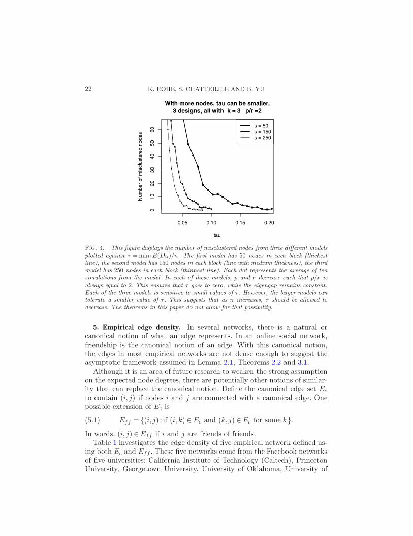
In this simulation, there are three different designs all from the four pa-rameter Stochastic Blockmodel. Each design has three blocks (k = 3). Onedesign contains 50 nodes in each block, another contains 150 in each block,and the last design contains 250 nodes in each block. To investigate howsensitive spectral clustering is to the value of τ = p/k+ r, the probabilities pand r must change. However, to isolate the effect of τ from the effect of
the eigengap (k(r/p) + 1)−2, it is necessary to keep the ratio p/r constant.Fixing p/r = 2 ensures that the eigengap is fixed at 4/25.
The results for Simulation 3 are displayed in Figure 3. The value τ is onthe horizontal axis, and the number of misclustered nodes is on the verticalaxis. There are three lines. The thickest line represents the design with 50nodes in each block. The line of medium thickness represents the design with150 nodes in each block. The thinnest line represents the design with 250nodes in each block. All three lines increase as τ approaches zero (reading thefigure from right to left). The thickest line starts to increase at τ = 0.20. Thethinnest line starts to increase at τ = 0.07. The line with medium thicknessincreases in between these two lines.
Because the thinner lines start to increase at a smaller value of τ , thissuggests that as n increase, τ can decrease. As such, spectral clusteringshould be able to correctly cluster the nodes in a Stochastic Blockmodelgraph when the minimum expected degree does not grow linearly with thenumber of nodes in the graph.
Lemma 2.1, Theorem 2.2, and Theorem 3.1 all require the minimum ex-pected degree to grow at the same rate as n (ignoring logn terms). Al-though the strict assumption is inappropriate for large networks, this simu-lation demonstrates (1) that spectral clustering works for smaller networksand (2) that the asymptotic theory presented earlier in the paper can bea guide to smaller networks. In these networks, it is not as unreasonablethat each node would be connected to a significant proportion of the othernodes.
22 K. ROHE, S. CHATTERJEE AND B. YU
Fig. 3. This figure displays the number of misclustered nodes from three different modelsplotted against τ = miniE(Dii)/n. The first model has 50 nodes in each block (thickestline), the second model has 150 nodes in each block (line with medium thickness), the thirdmodel has 250 nodes in each block (thinnest line). Each dot represents the average of tensimulations from the model. In each of these models, p and r decrease such that p/r isalways equal to 2. This ensures that τ goes to zero, while the eigengap remains constant.Each of the three models is sensitive to small values of τ . However, the larger models cantolerate a smaller value of τ . This suggests that as n increases, τ should be allowed todecrease. The theorems in this paper do not allow for that possibility.
5. Empirical edge density. In several networks, there is a natural orcanonical notion of what an edge represents. In an online social network,friendship is the canonical notion of an edge. With this canonical notion,the edges in most empirical networks are not dense enough to suggest theasymptotic framework assumed in Lemma 2.1, Theorems 2.2 and 3.1.
Although it is an area of future research to weaken the strong assumptionon the expected node degrees, there are potentially other notions of similar-ity that can replace the canonical notion. Define the canonical edge set Ec
to contain (i, j) if nodes i and j are connected with a canonical edge. Onepossible extension of Ec is
Eff = {(i, j) : if (i, k) ∈Ec and (k, j) ∈Ec for some k}.(5.1)
In words, (i, j) ∈Eff if i and j are friends of friends.Table 1 investigates the edge density of five empirical network defined us-
ing both Ec and Eff . These five networks come from the Facebook networksof five universities: California Institute of Technology (Caltech), PrincetonUniversity, Georgetown University, University of Oklahoma, University of
CLUSTERING FOR THE STOCHASTIC BLOCKMODEL 23
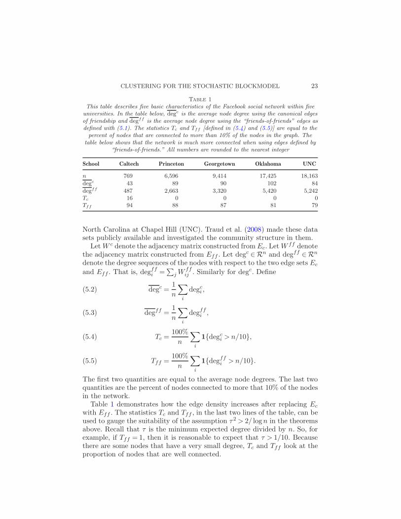
Table 1
This table describes five basic characteristics of the Facebook social network within fiveuniversities. In the table below, degc is the average node degree using the canonical edgesof friendship and degff is the average node degree using the “friends-of-friends” edges asdefined with (5.1). The statistics Tc and Tff [defined in (5.4) and (5.5)] are equal to thepercent of nodes that are connected to more than 10% of the nodes in the graph. The
table below shows that the network is much more connected when using edges defined by“friends-of-friends.” All numbers are rounded to the nearest integer
School Caltech Princeton Georgetown Oklahoma UNC
n 769 6,596 9,414 17,425 18,163
degc 43 89 90 102 84
degff 487 2,663 3,320 5,420 5,242Tc 16 0 0 0 0Tff 94 88 87 81 79
North Carolina at Chapel Hill (UNC). Traud et al. (2008) made these datasets publicly available and investigated the community structure in them.
LetW c denote the adjacency matrix constructed from Ec. LetWff denote
the adjacency matrix constructed from Eff . Let degc ∈Rn and degff ∈Rn
denote the degree sequences of the nodes with respect to the two edge sets Ec
and Eff . That is, degffi =
∑
j Wffij . Similarly for degc. Define
degc =1
n
∑
i
degci ,(5.2)
degff =1
n
∑
i
degffi ,(5.3)
Tc =100%
n
∑
i
1{degci > n/10},(5.4)
Tff =100%
n
∑
i
1{degffi > n/10}.(5.5)
The first two quantities are equal to the average node degrees. The last twoquantities are the percent of nodes connected to more that 10% of the nodesin the network.
Table 1 demonstrates how the edge density increases after replacing Ec
with Eff . The statistics Tc and Tff , in the last two lines of the table, can beused to gauge the suitability of the assumption τ2 > 2/ logn in the theoremsabove. Recall that τ is the minimum expected degree divided by n. So, forexample, if Tff = 1, then it is reasonable to expect that τ > 1/10. Becausethere are some nodes that have a very small degree, Tc and Tff look at theproportion of nodes that are well connected.
24 K. ROHE, S. CHATTERJEE AND B. YU
It is an empirical observation that graphs have sparse degrees. This sug-gests that the assumption τ2 > 2/ logn in Lemma 2.1, Theorem 2.2 andTheorem 3.1 is not satisfied in practice. Table 1 demonstrates that by usingan alternative notion of adjacency or connected, the network can becomemuch more connected.
6. Discussion. The goal of this paper is to bring statistical rigor to thestudy of community detection by assessing how well spectral clustering canestimate the clusters in the Stochastic Blockmodel. The Stochastic Block-model is easily amenable to the analysis of clustering algorithms because ofits simplicity and well-defined communities. The fact that spectral cluster-ing performs well on the Stochastic Blockmodel is encouraging. However,because the Stochastic Blockmodel fails to represent fundamental featuresthat most empirical networks display, this result should only be considereda first step.
This paper has two main results. The first main result, Theorem 2.2,proves that under the latent space model, the eigenvectors of the empiricalnormalized graph Laplacian converge to the eigenvectors of the populationnormalized graph Laplacian—so long as (1) the minimum expected degreegrows fast enough and (2) the eigengap that separates the leading eigenvaluesfrom the smaller eigenvalues does not shrink too quickly. This theorem hasconsequences in addition to those related to spectral clustering.
Visualization is an important tool for social networks analysts [Liotta(2004), Freeman (2000), Wasserman and Faust (1994)]. However, there islittle statistical understanding of these techniques under stochastic models.Two visualization techniques, factor analysis and multidimensional scaling,have variations that utilize the eigenvectors of the graph Laplacian. Similarapproaches were suggested for social networks as far back as the 1950s [Bockand Husain (1952), Breiger, Boorman and Arabie (1975)]. Koren (2005)suggests visualizing the graph using the eigenvectors of the unnormalizedgraph Laplacian. The analogous method for the normalized graph Laplacianwould use the ith row of X as the coordinates for the ith node. Theorem 2.2shows that, under the latent space model, this visualization is not muchdifferent than visualizing the graph by instead replacing X with X . If thereis structure in the latent space of a latent space model (e.g., the z1, . . . , znform clusters) and this structure is represented in the eigenvectors of thepopulation normalized graph Laplacian, then plotting the eigenvectors willpotentially reveal this structure.
The Stochastic Blockmodel is a specific latent space model that satisfiesthese conditions. It has well-defined clusters or blocks and Lemma 3.1 showsthat, under weak assumptions, the eigenvectors of the population normalizedgraph Laplacian perfectly identify the block structure. Theorem 2.2 suggeststhat you could discover this clustering structure by using the visualizationtechnique proposed by Koren (2005). The second main result, Theorem 3.1,
CLUSTERING FOR THE STOCHASTIC BLOCKMODEL 25
goes further to suggest just how many nodes you might miscluster by runningk-means on those points (this is spectral clustering). Theorem 3.1 provesthat if (1) the minimum expected degree grows fast enough and (2) thesmallest nonzero eigenvalue of the population normalized graph Laplacianshrinks slowly enough, then the proportion of nodes that are misclusteredby spectral clustering vanishes in the asymptote.
The asymptotic framework applied in Theorem 3.1 allows the numberof blocks to grow with the number of nodes; this is the first such high-dimensional clustering result. Allowing the number of clusters to grow isreasonable because as Leskovec et al. (2008) noted, large networks do notnecessarily have large communities. In fact, in a wide range of empiricalnetworks, the tightest communities have a roughly constant size. Allowingthe number of blocks to grow with the number of nodes ensures the clustersdo not become too large.
There are two main limitations of our results that are highlighted in thesimulations in Section 4. First, Theorem 3.1 does not show that spectral clus-tering is consistent under the Stochastic Blockmodel; it only gives a boundon the number of misclassified nodes. Improving this bound is an area forfuture research. The second shortcoming is that Lemma 2.1, Theorems 2.2and 3.1 all require the minimum expected degree to grow at the same rateas n (ignoring logn terms). In large empirical networks, the canonical edgesare not dense enough to suggest this type of asymptotic framework. Sec-tion 5 suggests alternative definitions of edges that might increase the edgedensity. That said, studying spectral clustering under more realistic degreedistributions is an area for future research.
APPENDIX A: PROOF OF THEOREM 2.1
First, a proof of Lemma 2.1.
Proof of Lemma 2.1. By eigendecomposition, M =∑n
i=1λiuiuTi whe-
re u1, . . . , un are orthonormal and eigenvectors of M . So,
MM =
(
n∑
i=1
λiuiuTi
)(
n∑
i=1
λiuiuTi
)
=n∑
i=1
λ2i uiu
Ti .
Right multiplying by any ui yields MMui = λ2ui. This proves one directionof part one in the lemma, if λ is an eigenvalue of M , then λ2 is an eigenvalueof MM . It also proves part two of the lemma, all eigenvectors of M are alsoeigenvectors of MM .
To see that if λ2 is an eigenvalue of MM , then λ or −λ is an eigenvalueof M , notice that both M and MM have exactly n eigenvalues (countingmultiplicities) because both matrices are real and symmetric. So, the pre-vious paragraph specifies n eigenvalues of MM by squaring the eigenvaluesofM . BecauseMM has exactly n eigenvalues, there are no other eigenvalues.

26 K. ROHE, S. CHATTERJEE AND B. YU
The rest of the proof is devoted to part three of the lemma. Let MMv =λ2v. By eigenvalue decomposition, M =
∑
i λiuiuTi and because u1, . . . , un
are orthonormal (M is real and symmetric) there exists α1, . . . , αn such thatv =
∑
iαiui.
λ2∑
i
αiui = λ2v =MMv =M
(
∑
i
λiuiuTi v
)
=M
(
∑
i
λiαiui
)
=∑
i
λiαiMui =∑
i
λ2iαiui.
By the orthogonality of the ui’s, it follows that λ2αi = λ2iαi for all i. So, if
λ2i 6= λ2, then αi = 0. �
For i= 1, . . . , n, define ci =Dii/n and τ =mini=1,...,n ci.
Lemma A.1. If n1/2/ logn> 2,
P
(
‖LL−L L ‖F ≥ 32√2 logn
τ2n1/2
)
≤ 4n2−2τ2 logn.
The main complication of the proof of Lemma A.1 is controlling the de-pendencies between the elements of LL. We do this with an intermediatestep that uses the matrix
L= D−1/2WD
−1/2
and two sets Γ and Λ. Γ constrains the matrix D, while Λ constrains the ma-trix WD−1W . These sets will be defined in the proof. To ease the notation,define
PΓΛ(B) = P(B ∩ Γ ∩Λ),
where B is some event.
Proof of Lemma A.1. This proof shows that under the sets Γ and Λthe probability of the norm exceeding 32
√2 log(n)τ−2n−1/2 is exactly zero
for large enough n and that the probability of Γ or Λ not happening isexponentially small. To ease notation, define a= 32
√2 log(n)τ−2n−1/2.
The diagonal terms behave differently than the off diagonal terms. So,break them apart:
P(‖LL−L L ‖F ≥ a)
≤ PΓΛ(‖LL−L L ‖F ≥ a) + P((Γ ∩Λ)c)
= PΓΛ
(
∑
i,j
[LL−L L ]2ij ≥ a2)
+ P((Γ ∩Λ)c)
CLUSTERING FOR THE STOCHASTIC BLOCKMODEL 27
≤ PΓΛ
(
∑
i 6=j
[LL−L L ]2ij ≥ a2/2
)
+ PΓΛ
(
∑
i
[LL−L L ]2ii ≥ a2/2
)
+ P((Γ∩Λ)c).
First, address the sum over the off diagonal terms:
PΓΛ
(
∑
i 6=j
[LL−L L ]2ij ≥ a2/2
)
≤ PΓΛ
(
⋃
i 6=j
{
[LL−L L ]2ij ≥a2
2n2
})
(A.1)
≤∑
i 6=j
PΓΛ
(
|LL−L L |ij ≥a√2n
)
≤∑
i 6=j
PΓΛ
(
|LL− LL|ij + |LL−L L |ij ≥a√2n
)
≤∑
i 6=j
[
PΓΛ
(
|LL− LL|ij ≥a√8n
)
+ PΓΛ
(
|LL−L L |ij ≥a√8n
)]
.(A.2)
The sum over the diagonal terms is similar,
PΓΛ
(
∑
i
[LL−L L ]2ii ≥ a2/2
)
≤∑
i
[
PΓΛ
(
|LL− LL|ii ≥a√8n
)
+ PΓΛ
(
|LL−L L |ii ≥a√8n
)]
with one key difference. In (A.1), the union bound address nearly n2 terms.This yields the 1/n2 term in line (A.1). After taking the square root, eachterm has a lower bound with a factor of 1/n. However, because there areonly n terms on the diagonal, after taking the square root in the last equation
above, the lower bound has a factor of 1/√n.
To constrain the terms |LL−L L |ij for i= j and i 6= j, define
Λ =⋂
i,j
{∣
∣
∣
∣
∑
k
(WikWjk − pijk)/ck
∣
∣
∣
∣
< n1/2 logn
}
,
28 K. ROHE, S. CHATTERJEE AND B. YU
where
pijk =
{
pikpjk, if i 6= j,pik, if i= j,
for pij =Wij . We now show that for large enough n and any i 6= j,
PΛ
(
|LL−L L |ij ≥a√8n
)
= 0,(A.3)
PΛ
(
|LL−L L |ii ≥a√8n
)
= 0.(A.4)
To see (A.3), expand the left-hand side of the inequality for i 6= j,
|LL−L L |ij =1
(DiiDjj)1/2
∣
∣
∣
∣
∑
k
(WikWjk − pikpjk)/Dkk
∣
∣
∣
∣
=1
n2√cicj
∣
∣
∣
∣
∑
k
(WikWjk − pikpjk)/ck
∣
∣
∣
∣
.
This is bounded on Λ, yielding
|LL−L L |ij <logn
τn3/2≤ 32
√2 logn√
8τ2n3/2=
a√8n
.
So, (A.3) holds for i 6= j. Equation (A.4) is different because W 2ik =Wik. As
a result, the diagonal of LL is a biased estimator of the diagonal of L L .
|LL−L L |ii =∣
∣
∣
∣
∑
k
W 2ik − p2ik
DiiDkk
∣
∣
∣
∣
=
∣
∣
∣
∣
∑
k
Wik − p2ikDiiDkk
∣
∣
∣
∣
≤∣
∣
∣
∣
∑
k
Wik − pikDiiDkk
∣
∣
∣
∣
+
∣
∣
∣
∣
∑
k
pik − p2ikDiiDkk
∣
∣
∣
∣
(A.5)
=1
cin2
(∣
∣
∣
∣
∑
k
(Wik − pik)/ck
∣
∣
∣
∣
+
∣
∣
∣
∣
∑
k
(pik − p2ik)/ck
∣
∣
∣
∣
)
.
Similar to the i 6= j case, the first term is bounded by log(n)τ−1n−3/2 on Λ.The second term is bounded by τ−2n−1:
1
cin2
∣
∣
∣
∣
∑
k
(pik − p2ik)/ck
∣
∣
∣
∣
≤ 1
cin2
∣
∣
∣
∣
∑
k
1/τ
∣
∣
∣
∣
≤ 1
τ2n.
Substituting the value of a in reveals that on the set Λ, both terms in (A.5)are bounded by a(2
√8n)−1. So, their their sum is bounded by a(
√8n)−1,
satisfying (A.4).
CLUSTERING FOR THE STOCHASTIC BLOCKMODEL 29
This next part addresses the difference between LL and LL, showing thatfor large enough n, any i 6= j, and some set Γ,
PΓΛ
(
|LL− LL|ij ≥a√8n
)
= 0,
PΓΛ
(
|LL− LL|ii ≥a√8n
)
= 0.
It is enough to show that for any i and j,
PΓΛ
(
|LL− LL|ij ≥a√8n
)
= 0.(A.6)
For b(n) = log(n)n−1/2, define u(n) = 1+ b(n), l(n) = 1− b(n). With thesedefine the following sets:
Γ =⋂
i
{Dii ∈Dii[l(n), u(n)]},
Γ(1) =⋂
i
{
1
Dii∈ 1
Dii[u(n)−1, l(n)−1]
}
,
Γ(2) =⋂
i,j
{
1
(DiiDjj)1/2∈ 1
(DiiDjj)1/2[u(n)−1, l(n)−1]
}
,
Γ(3) =⋂
i,j,k
{
1
Dkk(DiiDjj)1/2∈ [u(n)−2, l(n)−2]
Dkk(DiiDjj)1/2
}
.
Notice that Γ⊆ Γ(1)⊆ Γ(2) and Γ⊆ Γ(3). Define another set:
Γ(4) =⋂
i,j,k
{
1
Dkk(DiiDjj)1/2∈ [1− 16b(n),1 + 16b(n)]
Dkk(DiiDjj)1/2
}
.
The next steps show that this set contains Γ. It is sufficient to show Γ(3)⊂Γ(4). This is true because
1
u(n)2=
1
(1 + b(n))2=
b(n)−2
(b(n)−1 +1)2>
b(n)−2 − 1
(b(n)−1 + 1)2
=b(n)−1 − 1
b(n)−1 +1= 1− 2
b(n)−1 +1> 1− 16b(n).
The 16 in the last bound is larger than it needs to be so that the upper andlower bounds in Γ(4) are symmetric. For the other direction,
1
l(n)2=
1
(1− b(n))2=
b(n)−2
(b(n)−1 − 1)2=
(
1 +1
b(n)−1 − 1
)2
= 1+2
b(n)−1 − 1+
1
(b(n)−1 − 1)2.
30 K. ROHE, S. CHATTERJEE AND B. YU
We now need to bound the last two elements here. We are assuming,√n/ logn> 2. Equivalently, 1−b(n)> 1/2. So, we have both of the following:
1
(b(n)−1 − 1)2<
2
b(n)−1 − 1and
2
b(n)−1 − 1=
2b(n)
1− b(n)< 8b(n).
Putting these together,
1
l(n)2< 1 + 16b(n).
This shows that Γ⊂ Γ(4). Now, under the set Γ, and thus Γ(4),
|LL− LL|ij =∣
∣
∣
∣
∑
k
(
WikWjk
Dkk(DiiDjj)1/2− WikWjk
Dkk(DiiDjj)1/2
)∣
∣
∣
∣
≤∑
k
∣
∣
∣
∣
1
Dkk(DiiDjj)1/2− 1
Dkk(DiiDjj)1/2
∣
∣
∣
∣
≤∑
k
∣
∣
∣
∣
16b(n)
Dkk(DiiDjj)1/2
∣
∣
∣
∣
≤∑
k
16b(n)
τ2n2≤ 16b(n)
τ2n.
This is equal to a(√8n)−1, showing (A.4) holds for all i and j.
The remaining step is to bound P((Γ∩Λ)c). Using the union bound, thisis less than or equal to P(Γc) + P(Λc):
P(Γc) = P
(
⋃
i
{Dii /∈ Dii[1− b(n),1 + b(n)]})
≤∑
i
P({Dii /∈Dii[1− b(n),1 + b(n)]})
<∑
i
2exp
(
−2
(
Dii logn√n
)2 1
n
)
≤ 2n exp(−2τ2(logn)2)
= 2n1−2τ2 logn,
where the second to last inequality is by Hoeffding’s inequality. The nextinequality is Hoeffding’s:
P(Λc) = P
(
⋃
i,j
{∣
∣
∣
∣
∑
k
(WikWjk − pijk)/ck
∣
∣
∣
∣
> n1/2 logn
})
=∑
i,j
P
(∣
∣
∣
∣
∑
k
(WikWjk − pijk)/ck
∣
∣
∣
∣
> n1/2 logn
)

CLUSTERING FOR THE STOCHASTIC BLOCKMODEL 31
<∑
i,j
2exp
(
−2n(logn)2/
∑
k
1/c2k
)
≤∑
i,j
2exp(−2(logn)2τ2)
≤ 2n2 exp(−2(logn)2τ2)
≤ 2n2−2τ2 logn.
Because W is symmetric, the independence of the WikWjk across k is notobvious. However, because Wii =Wjj = 0, they are independent across k.
Putting the pieces together,
P
(
‖LL−L L ‖F ≥ 32√2 logn
τ2n1/2
)
≤ PΓΛ
(
‖LL−L L ‖F ≥ 32√2 logn
τ2n1/2
)
+ P((Γ ∩Λ)c)
< 0 + 2n1−2τ2 logn +2n2−2τ2 logn
≤ 4n2−2τ2 logn. �
The following proves Theorem 2.1.
Proof of Theorem 2.1. Adding the n super- and subscripts to Lem-ma A.1, it states that if n1/2/ logn> 2, then
P
(
‖LL−L L ‖F ≥ c logn
τ2n1/2
)
< 4n2−2τ2 logn
for c= 32√2. By assumption, for all n > N , τ2n logn > 2. This implies that
2− 2τ2n logn <−2 for all n >N . Rearranging and summing over n, for anyfixed ε > 0,
∞∑
n=1
P
(‖L(n)L(n) −L (n)L (n)‖Fcτ−2
n log(n)n−1/2/ε≥ ε
)
≤N +4∞∑
n=N+1
n2−2τ2n logn
≤N +4∞∑
n=N+1
n−2,
which is a summable sequence. By the Borel–Cantelli theorem,
‖L(n)L(n) −L(n)
L(n)‖F = o(τ−2
n log(n)n−1/2) a.s. �

32 K. ROHE, S. CHATTERJEE AND B. YU
APPENDIX B: DAVIS–KAHAN THEOREM
The statement of the theorem below and the preceding explanation comelargely from von Luxburg (2007). For a more detailed account of the Davis–Kahan theorem, see Stewart and Sun (1990).
To avoid the issues associated with multiple eigenvalues, this theorem’soriginal statement is instead about the subspace formed by the eigenvec-tors. For a distance between subspaces, the theorem uses “canonical angles,”which are also known as “principal angles.” Given two matrices M1 and M2
both in Rn×p with orthonormal columns, the singular values (σ1, . . . , σp)of M ′
1M2 are the cosines of the principal angles (cosΘ1, . . . , cosΘp) betweenthe column space of M1 and the column space of M2. Define sinΘ(M1,M2)to be a diagonal matrix containing the sine of the principal angles of M ′
1M2
and define
d(M1,M2) = ‖sinΘ(M1,M2)‖F ,(B.1)
which can be expressed as (p −∑pj=1 σ
2j )
1/2 by using the identity sin2 θ =
1− cos2 θ.
Proposition B.1 (Davis–Kahan). Let S ⊂R be an interval. Denote Xas an orthonormal matrix whose column space is equal to the eigenspaceof L L corresponding to the eigenvalues in λS(L L ) [more formally, thecolumn space of X is the image of the spectral projection of L L induced byλS(L L )]. Denote by X the analogous quantity for LL. Define the distancebetween S and the spectrum of L L outside of S as
δ =min{|λ− s|;λ eigenvalue of L L , λ /∈ S, s ∈ S}.Then the distance d(X ,X) = ‖sinΘ(X ,X)‖F between the column spaces of Xand X is bounded by
d(X,X )≤ ‖LL−L L ‖Fδ
.
In the theorem, L L and LL can be replaced by any two symmetric ma-trices. The rest of this section converts the bound on d(X,X ) to a bound on‖X −XO‖F , where O is some orthonormal rotation. For this, we will makean additional assumption that X and X have the same dimension. Assumethere exists S ⊂ R containing k eigenvalues of L L and k eigenvalues ofLL, but containing no other eigenvalues of either matrix. Because LL andL L are symmetric, its eigenvectors can be defined to be orthonormal. Letthe columns of X ∈ Rn×k be k orthonormal eigenvectors of L L corre-sponding to the k eigenvalues contained in S. Let the columns of X ∈Rn×k
be k orthonormal eigenvectors of LL corresponding to the k eigenvalues con-tained in S. By singular value decomposition, there exist orthonormal matri-ces U,V and diagonal matrix Σ such that X TX = UΣV T . The singular
CLUSTERING FOR THE STOCHASTIC BLOCKMODEL 33
values, σ1, . . . , σk, down the diagonal of Σ are the cosines of the principalangles between the columns space of X and the column space of X .
Although the Davis–Kahan theorem is a statement regarding the principalangles, a few lines of algebra show that it can be extended to a bound on theFrobenius norm between the matrix X and X UV T , where the matrix UV T
is an orthonormal rotation:
1
2‖X −X UV T ‖2F =
1
2trace((X −X UV T )T (X −X UV T ))
=1
2trace(V UT
XTX UV T +XTX − 2V UT
XTX)
=1
2(k+ k− 2 trace(V UT
XTX))
≤ ‖LL−L L ‖2Fδ2
,
where the last inequality is explained below. It follows from a property ofthe trace, the fact that the singular values are in [0,1], the trigonometricidentity cos2 θ = 1− sin2 θ and the Davis–Kahan theorem:
trace(V UTX
TX) =
k∑
i=1
σi ≥k∑
i=1
(cosΘi)2 =
k∑
i=1
1− (sinΘi)2
= k− (d(X,X ))2 ≥ k− ‖LL−L L ‖2Fδ2
.
This shows that the Davis–Kahan theorem can instead be thought of asa bounding ‖X UV T −X‖2F instead of d(X ,X). The matrix O in Theo-rem 2.1 is equal to UV T . In this way, it is dependent on X and X .
APPENDIX C: PROOF OF THEOREM 2.2
By Lemma 2.1, the column vectors of Xn are eigenvectors of L(n)L(n)
corresponding to all the eigenvalues in λSn(L(n)L(n)). For the application
of the Davis–Kahan theorem, this means that the column space of Xn isthe image of the spectral projection of L(n)L(n) induced by λSn(L
(n)L(n)),similarly for the column vectors of Xn, the matrix L (n)L (n) and the setλSn(L
(n)L (n)).
Recall that λ(n)1 ≥ · · · ≥ λ
(n)n are defined to be the eigenvalues of symmetric
matrix L (n)L (n) and λ(n)1 ≥ · · · ≥ λ
(n)n are defined to be the eigenvalues of
symmetric matrix L(n)L(n). From (2.2),
maxi
|λ(n)i − λ
(n)i |= o
(
logn
τ2nn1/2
)
.
34 K. ROHE, S. CHATTERJEE AND B. YU
By assumption, τ2n > 2/ logn. So,
logn
τ2nn1/2
<(logn)2
2n1/2=O(min{δn, δ′n}),
where the last step follows by assumption. Thus,
maxi
|λ(n)i − λ
(n)i |= o(min{δn, δ′n}).
This means that, eventually, λ(n)i ∈ Sn if and only if λ
(n)i ∈ Sn. Thus, the
number of elements in λSn(L(n)L (n)) is eventually equal to the number of
elements in λSn(L(n)L(n)) implying that Xn and Xn will eventually have
the same number of columns, kn =Kn.Once Xn and Xn have the same number of columns, define matrices Un
and Vn with singular value decomposition: X Tn Xn = UnΣnV
Tn . Define On =
UnVTn . The result follows from the Davis–Kahan theorem and Theorem 2.1:
‖Xn −XnOn‖F ≤ 2‖L(n)L(n) −L (n)L (n)‖Fδn
= o
(
logn
δnτ2nn1/2
)
a.s.
APPENDIX D: STOCHASTIC BLOCKMODEL
Proof of Lemma 3.1. First, construct the matrix BL ∈ Rk×k suchthat L = ZBLZ
T . Define DB = diag(BZT1n) ∈Rk×k where 1n is a vector
of ones in Rn. For any i, j,
Lij =Wij
√
DiiDjj
= ziD−1/2B BD
−1/2B (zj)
T .
Define BL =D−1/2B BD
−1/2B . It follows that Lij = (ZBLZ
T )ij and thus L =ZBLZ
T .Because B is symmetric, so are BL and (ZTZ)1/2BL(Z
TZ)1/2. Noticethat
det((ZTZ)1/2BL(ZTZ)1/2) = det((ZTZ)1/2)det(BL)det((Z
TZ)1/2)> 0.
By eigenvector decomposition, define V ∈ Rk×k and diagonal matrix Λ ∈Rk×k such that
(ZTZ)1/2BL(ZTZ)1/2 = V ΛV T .(D.1)
Because the determinant of the left-hand side of (D.1) is greater than zero,none of the eigenvalues in Λ are equal to zero. Left multiply (D.1) byZ(ZTZ)−1/2 and right multiply by (ZTZ)−1/2ZT . This shows
ZBLZT = ZµΛ(Zµ)T ,(D.2)
where µ = (ZTZ)−1/2V . Notice that (Zµ)T (Zµ) = Ik, the k × k identitymatrix. So, right multiplying (D.2) by Zµ shows that the columns of Zµ are

CLUSTERING FOR THE STOCHASTIC BLOCKMODEL 35
eigenvectors of ZBLZT = L with the eigenvalues down the diagonal of Λ.
Equation (D.2) shows that these are the only nonzero eigenvalues.It remains to prove equivalence statement (3.2). Notice
det(µ) = det((ZTZ)−1/2)det(V )> 0.
So, µ−1 exists and statement (3.2) follows. �
The following is a proof of Lemma 3.2.
Proof of Lemma 3.2. The following statement is the essential ingre-dient to prove Lemma 3.2.
zi 6= zj then ‖ziµ− zjµ‖2 ≥√
2/P .(D.3)
The proof of statement (D.3) requires the following definition:
‖µ‖2m = minx : ‖x‖2=1
‖xµ‖22.
Notice that
‖µ‖2m = minx : ‖x‖2=1
xµµTxT = minx : ‖x‖2=1
x(ZTZ)−1xT = 1/P.
So,
‖ziµ− zjµ‖2 = ‖(zi − zj)µ‖2 ≥√2‖µ‖m =
√
2/P .
Proving statement (D.3). The proof of Lemma 3.2 follows:
‖ciO− zjµ‖2 ≥ ‖ziµ− zjµ‖2 − ‖ciO− ziµ‖2 ≥√
2
P− 1
2
√
2
P=
1√2P
.�
Proof of Theorem 3.1. Define X ∈Rn×k to contain the eigenvectorsof L corresponding to the largest k eigenvalues and define
C = argminM∈R(n,k)
‖X −M‖2F ,
where R(n,k) is defined as:
R(n,k) = {M ∈Rn×k :M has no more than k unique rows}.Notice that
minM∈R(n,k)
‖X −M‖2F = min{m1,...,mk}⊂Rk
∑
i
ming
‖xi −mg‖22.
This shows that the ith row of C is equal to ci as defined in Definition 3.Because ZµO ∈ R(n,k), notice that
‖X −C‖2 ≤ ‖X −ZµO‖2.(D.4)
By the triangle inequality and inequality D.4,
‖C −ZµO‖2 ≤ ‖C −X‖2 + ‖X −ZµO‖2 ≤ 2‖X −ZµO‖2.
36 K. ROHE, S. CHATTERJEE AND B. YU
In the notation of Theorem 2.2, define Sn = [λ2kn/2,2]. Then, δ = δ′ =
λ2kn/2. By assumption, n−1/2(logn)2 =O(λ2
kn) =O(min{δ, δ′}). This implies
that the results from Theorem 2.2 hold. Putting the pieces together,
|M | ≤∑
i∈M
1≤ 2Pn
∑
i∈M
‖ci − ziµO‖22
≤ 2Pn‖C −ZµO‖2F≤ 8Pn‖X −ZµO‖2F
= o
(
Pn(logn)2
nλ4knτ4n
)
a.s.�
In the second example of Section 3, it was claimed that
λk =1
k(r/p) + 1.
The following is a proof of that statement.Define B ∈Rk×k such that
B = pIk + r1k1Tk ,
where Ik ∈Rk×k is the identity matrix, 1k ∈Rk is a vector of ones, r ∈ (0,1)and p ∈ (0,1− r). Assume that p and r are fixed and k can grow with n.Let Z ∈ {0,1}n×k be such that ZT
1n = s1k. This guarantees that all kgroups have equal size s. The Stochastic Blockmodel in the second exampleof Section 3 has the population adjacency matrix, W =ZBZT .
Define
BL =1
nr+ sp(pIk + r1k1
Tk ).
From the argument in the proof of Lemma 3.1, L has the same nonzero
eigenvalues as (ZTZ)1/2BL(ZTZ)1/2 ∈Rk×k. Let λ1, . . . , λk be the eigenval-
ues of (ZTZ)1/2BL(ZTZ)1/2 = (s1/2Ik)BL(s
1/2Ik) = sBL. Notice that 1k isan eigenvector with eigenvalue 1:
sBL1k =s
nr+ sp(pIk + r1k1
Tk )1k =
s(p+ kr)
nr+ sp1k = 1k.
Let λ1 = 1. Define
U = {u :‖u‖2 = 1, uT1= 0}.Notice that for all u ∈ U ,
sBLu=s
nr+ sp(pIk + r1k1
Tk )u=
sp
nr+ spu.(D.5)
CLUSTERING FOR THE STOCHASTIC BLOCKMODEL 37
Equation (D.5) implies that for i > 1,
λi =sp
nr+ sp.
This is also true for i= k.
λk =sp
nr+ sp=
sp
nr+ sp=
1
k(r/p) + 1.
This is the smallest nonzero eigenvalue of L .
Acknowledgments. The authors are grateful to Michael Mahoney andBenjamin Olding for their stimulating discussions. Also, thank you to JinzhuJia and Reza Khodabin for your helpful comments and suggestions on thispaper.
REFERENCES
Airoldi, E. M., Blei, D. M., Fienberg, S. E. and Xing, E. P. (2008). Mixed mem-bership stochastic blockmodels. J. Mach. Learn. Res. 9 1981–2014.
Albert, R. and Barabasi, A. L. (2002). Statistical mechanics of complex networks. Rev.Modern Phys. 74 47–97. MR1895096
Barabasi, A. L. and Albert, R. (1999). Emergence of scaling in random networks.Science 286 509–512. MR2091634
Belkin, M. (2003). Problems of learning on manifolds. Ph.D. thesis, Univ. Chicago.Belkin, M. and Niyogi, P. (2003). Laplacian eigenmaps for dimensionality reduction
and data representation. Neural Comput. 15 1373–1396.Belkin, M. and Niyogi, P. (2008). Towards a theoretical foundation for Laplacian-based
manifold methods. J. Comput. System Sci. 74 1289–1308. MR2460286Bhatia, R. (1987). Perturbation Bounds for Matrix Eigenvalues. Longman, Harlow.
MR0925418Bickel, P. J. and Chen, A. (2009). A nonparametric view of network models and
Newman–Girvan and other modularities. Proc. Nat. Acad. Sci. India Sect. A 106 21068.Bock, R. D. and Husain, S. (1952). Factors of the Tele: A preliminary report. Sociometry
15 206–219.Bousquet, O., Chapelle, O. and Hein, M. (2004). Measure based regularization. Adv.
Neural Inf. Process. Syst. 16.Brandes, U., Delling, D., Gaertler, M., Gorke, R., Hoefer, M., Nikoloski, Z.
and Wagner, D. (2008). On modularity clustering. IEEE Transactions on Knowledgeand Data Engineering 20 172–188.
Breiger, R. L., Boorman, S. A. and Arabie, P. (1975). An algorithm for cluster-ing relational data with applications to social network analysis and comparison withmultidimensional scaling. J. Math. Psych. 12 328–383.
Champion, M. (1998). How many atoms make up the universe? Available at http://
www.madsci.org/posts/archives/oct98/905633072.As.r.html.Choi, D., Wolfe, P. and Airoldi, E. (2010). Stochastic blockmodels with growing
number of classes. Preprint. Available at arXiv:1011.4644.Coifman, R., Lafon, S., Lee, A., Maggioni, M., Nadler, B., Warner, F. and
Zucker, S. (2005). Geometric diffusions as a tool for harmonic analysis and structuredefinition of data: Diffusion maps. Proc. Nat. Acad. Sci. India Sect. A 102 7426–7431.

38 K. ROHE, S. CHATTERJEE AND B. YU
Condon, A. and Karp, R. M. (1999). Algorithms for graph partitioning on the plantedpartition model. In Randomization, Approximation, and Combinatorial Optimization
(Berkeley, CA, 1999). Lecture Notes in Comput. Sci. 1671 221–232. Springer, Berlin.MR1775522
Donath, W. E. and Hoffman, A. J. (1973). Lower bounds for the partitioning of graphs.
IBM J. Res. Develop. 17 420–425. MR0329965Erdos, P. and Renyi, A. (1959). On random graphs. Publ. Math. Debrecen 6 290–297.
Fiedler, M. (1973). Algebraic connectivity of graphs. Czechoslovak Math. J. 23 298–305.MR0318007
Fjallstrom, P. (1998). Algorithms for graph partitioning: A survey. Computer and In-
formation Science 3. Available at http://www.ep.liu.se/ea/cis/1998/010/.Fortunato, S. (2010). Community detection in graphs. Phys. Rep. 486 75–174.
MR2580414Frank, O. and Strauss, D. (1986). Markov graphs. J. Amer. Statist. Assoc. 81 832–842.
MR0860518
Freeman, L. C. (2000). Visualizing social networks. Journal of Social Structure 1(1).Gine, E. and Koltchinskii, V. (2006). Empirical graph Laplacian approximation of
Laplace–Beltrami operators: Large sample results. In High Dimensional Probability.Institute of Mathematical Statistics Lecture Notes—Monograph Series 51 238–259. IMS,Beachwood, OH. MR2387773
Girvan, M. and Newman, M. (2002). Community structure in social and biological net-works. Proc. Nat. Acad. Sci. India Sect. A 99 7821–7826. MR1908073
Goldenberg, A., Zheng, A. X., Fienberg, S. E. and Airoldi, E. M. (2010). A surveyof statistical network models. Foundations and Trends in Machine Learning 2 129–233.
Hagen, L. and Kahng, A. B. (1992). New spectral methods for ratio cut partitioning
and clustering. IEEE Trans. Computer-Aided Design 11 1074–1085.Handcock, M. S., Raftery, A. E. and Tantrum, J. M. (2007). Model-based clustering
for social networks. J. Roy. Statist. Soc. Ser. A 170 301–354. MR2364300Hein, M. (2006). Uniform convergence of adaptive graph-based regularization. In Learning
Theory. Lecture Notes in Comput. Sci. 4005 50–64. Springer, Berlin. MR2277918
Hein, M., Audibert, J. Y. and von Luxburg, U. (2005). From graphs to manifolds—weak and strong pointwise consistency of graph Laplacians. In Learning Theory. Lecture
Notes in Comput. Sci. 3559 470–485. Springer, Berlin. MR2203281Hendrickson, B. and Leland, R. (1995). An improved spectral graph partitioning
algorithm for mapping parallel computations. SIAM J. Sci. Comput. 16 452–469.
MR1317066Hoff, P. D., Raftery, A. E. and Handcock, M. S. (2002). Latent space approaches
to social network analysis. J. Amer. Statist. Assoc. 97 1090–1098. MR1951262Holland, P., Laskey, K. B. and Leinhardt, S. (1983). Stochastic blockmodels: Some
first steps. Social Networks 5 109–137. MR0718088
Holland, P. W. and Leinhardt, S. (1981). An exponential family of probability distri-butions for directed graphs. J. Amer. Statist. Assoc. 76 33–50. MR0608176
Kallenberg, O. (2005). Probabilistic Symmetries and Invariance Principles. Springer,New York. MR2161313
Klein, D. and Randic, M. (1993). Resistance distance. J. Math. Chem. 12 81–95.
MR1219566Koren, Y. (2005). Drawing graphs by eigenvectors: Theory and practice. Comput. Math.
Appl. 49 1867–1888. MR2154691Lafon, S. S. (2004). Diffusion maps and geometric harmonics. Ph.D. thesis, Yale Univ.

CLUSTERING FOR THE STOCHASTIC BLOCKMODEL 39
Leskovec, J., Lang, K. J., Dasgupta, A. and Mahoney, M. W. (2008). Statisticalproperties of community structure in large social and information networks. In Proceed-ing of the 17th International Conference on World Wide Web 695–704. ACM, Beijing,China.
Liotta, G., ed. (2004). Graph Drawing. Lecture Notes in Comput. Sci. 2912. Springer,Berlin. MR2177577
Meila, M. and Shi, J. (2001). A random walks view of spectral segmentation. In AI andStatistics (AISTATS) 2001.
Newman, M. and Girvan, M. (2004). Finding and evaluating community structure innetworks. Phys. Rev. E (3) 69 026113.
Nowicki, K. and Snijders, T. A. B. (2001). Estimation and prediction for stochasticblockstructures. J. Amer. Statist. Assoc. 96 1077–1087. MR1947255
Pothen, A., Simon, H. D. and Liou, K. P. (1990). Partitioning sparse matrices witheigenvectors of graphs. SIAM J. Matrix Anal. Appl. 11 430–452. MR1054210
Shi, J. and Malik, J. (2000). Normalized cuts and image segmentation. IEEE Transac-tions on Pattern Analysis and Machine Intelligence 22 888–905.
Snijders, T. A. B. and Nowicki, K. (1997). Estimation and prediction for stochas-tic blockmodels for graphs with latent block structure. J. Classification 14 75–100.MR1449742
Spielman, D. A. and Teng, S. H. (2007). Spectral partitioning works: Planar graphsand finite element meshes. Linear Algebra Appl. 421 284–305. MR2294342
Steinhaus, H. (1956). Sur la division des corp materiels en parties. Bull. Acad. Polon.Sci. Cl. III 4 801–804. MR0090073
Stewart, G. W. and Sun, J. (1990). Matrix Perturbation Theory. Academic Press, SanDiego, CA.
Traud, A. L., Kelsic, E. D., Mucha, P. J. and Porter, M. A. (2008). Communitystructure in online collegiate social networks. Preprint.
Van Driessche, R. and Roose, D. (1995). An improved spectral bisection algorithm andits application to dynamic load balancing. Parallel Comput. 21 29–48. MR1314376
Van Duijn, M. A. J., Snijders, T. A. B. and Zijlstra, B. J. H. (2004). p2: A randomeffects model with covariates for directed graphs. Stat. Neerl. 58 234–254. MR2064846
von Luxburg, U. (2007). A tutorial on spectral clustering. Stat. Comput. 17 395–416.MR2409803
von Luxburg, U., Belkin, M. and Bousquet, O. (2008). Consistency of spectral clus-tering. Ann. Statist. 36 555–586. MR2396807
Vu, V. (2011). Singular vectors under random perturbation. Random Structures Algo-rithms. DOI:10.1002/rsa.20367.
Wasserman, S. and Faust, K. (1994). Social Network Analysis: Methods and Applica-tions. Cambridge Univ. Press, Cambridge.
Watts, D. J. and Strogatz, S. H. (1998). Collective dynamics of ‘small world’ networks.Nature 393 440–442.
Department of Statistics
University of California
Berkeley, California 94720
USA
E-mail: [email protected]@[email protected]