Spectral Bloom Filters

Saar Cohen Yossi MatiasSchool of Computer Science,

Tel Aviv University{saarco,matias}@cs.tau.ac.il

Abstract

A Bloom Filter is a space-efficient randomized data structure allowing membership queries oversets with certain allowable errors. It is widely used in many applications which take advantage ofits ability to compactly represent a set, and filter out effectively any element that does not belongto the set, with small error probability. This report introduces the Spectral Bloom Filter (SBF),an extension of the original Bloom Filter to multi-sets, allowing the filtering of elements whosemultiplicities are below a threshold given at query time. Using memory only slightly larger thanthat of the original Bloom Filter, the SBF supports queries on the multiplicities of individual keyswith a guaranteed, small error probability. The SBF also supports insertions and deletions overthe data set. We present novel methods for reducing the probability and magnitude of errors.We also present an efficient data structure (the String-array index ), and algorithms to build itincrementally and maintain it over streaming data, as well as over materialized data with arbitraryinsertions and deletions. The SBF does not assume any a priori filtering threshold and effectivelyand efficiently maintains information over the entire data-set, allowing for ad-hoc queries witharbitrary parameters and enabling a range of new applications.

The SBF, and the String-array index data structure are both efficient and fairly easy to imple-ment, which make them a very practical solution to situation in which filtering of a given spectrumare necessary. The methods proposed and the data structure were fully implemented and testedunder various conditions, testing their accuracy, memory requirements and speed of execution.Those experiments are reported within this report, as well as analysis of the expected behavior forseveral common scenarios.

1 Introduction

Bloom Filters are space efficient data structures which allow for membership queries over a givenset [Blo70]. The Bloom Filter uses k hash functions, h1, h2, . . . , hk to hash elements from a set Sinto an array of size m. For each element s ∈ S, the bits at positions h1(s), h2(s), . . . , hk(s) inthe array are set to 1. Given an item q, we check its membership in S by examining the bits atpositions h1(q), h2(q), . . . , hk(q). The item q is reported to be in S if (and only if) all the bits areset to 1. This method allows a small probability of a false positive error (it may return a positiveresult for an item which actually is not contained in S), but no false-negative error, while gainingsubstantial space savings. Bloom Filters are widely used in many applications.

This report introduces the Spectral Bloom Filter (SBF), an extension of the original BloomFilter to multi-sets, allowing estimates of the multiplicities of individual keys with a small errorprobability. This expansion of the Bloom Filter is spectral in the sense that it allows filtering of

1

elements whose multiplicities are within a requested spectrum. The SBF extends the functionalityof the Bloom Filter and thus makes it usable in a variety of new applications, while requiring onlya slight increase in memory compared to the original Bloom Filter. We present efficient algorithmsto build an SBF, and maintain it for streaming data, as well as arbitrary insertions and deletions.The SBF can be considered as a high-granularity histogram. It is considerably larger than regularhistograms, but unlike such histograms it supports queries at high granularity, and in fact at thesingle item level, and it is substantially smaller than the original data set.

Unlike the standard Bloom Filter, which uses a straight-forward approach to storage (a bitvector), the SBF is by nature more complex. Since counters have to be stored in an economicalfashion, a major consideration is the ability to hold, update and access the information in an efficientand compact manner. To do so, this report presents the String-Array Index data structure, fulfillingthese requirements. We also propose and analyze methods for querying the SBF, improving overthe standard lookup scheme and reducing the error probability and size.

1.1 Previous work

As the size of data sets encountered in databases, in communication, and in other applicationskeeps on growing, it becomes increasingly important to handle massive data sets using compactdata structures. Indeed, there is extensive research in recent years on data synopses [GM99] anddata streams [AMS99, BBD+02].

The applicability of Bloom Filters as an effective, compact data representation is well recog-nized. In this section, we briefly survey several major applications of Bloom Filters. These usesinclude peer-to-peer systems, distributed calculations and distributed database queries and otherapplications. Several modifications have also been published over the basic Bloom Filter structure,optimizing the performance and storage for different scenarios.

1.1.1 Distributed processing

Bloom Filters are often used in distributed environments to store an inventory of items storedat every node. In [FCAB98], Bloom Filters are proposed to be used within a hierarchy of proxyservers to maintain a summary of the data stored in the cache of each proxy. This allows for ascalable caching scheme utilizing several servers. The Summary Cache algorithm proposed in thesame paper was implemented in the Squid web proxy cache software [FCA, Squ], with a variationof this algorithm called Cache Digest implemented in a later version of Squid. In this scenario, theBloom Filters are exchanged between nodes, creating an efficient method of representing the fullpicture of the items stored in every proxy among all proxies.

In peer-to-peer systems, an efficient algorithm is needed to establish the nearest node holdinga copy of a requested file, and the route to reach it. In [RK02], a structure called “AttenuatedBloom Filter” is described. This structure is basically an array of simple Bloom Filters in whichcomponent filters are labeled with their level in the array. Each filter summarizes the items thatcan be reached by performing a number of hops from the originating node that is equal to thelevel of that filter. The paper proposes an algorithm for efficient location of information using thisstructure. The main difference between this method and the Summary Cache algorithm is that inthis article, the notion of distance and route between nodes is taken into consideration, while in[FCAB98], every remote node reachable (and whose data is maintained) in every node is consideredto be within the same distance from the originating node.

A different aspect of distributed processing is distributed database systems. In such system,the data is partitioned and stored in several locations. Usually, the scenario in question involves

2

several relations which reside on different locations, and a query that requires a join between thoserelations. The use of Bloom Filters was proposed in handling such joins. Bloomjoin is a scheme forperforming distributed joins [ML86], in which a join between relations R and S over the attributeX is handled by building a Bloom Filter over R.X and transmitting it to S. This Bloom Filter isused to filter tuples in S which will not contribute to the join result, and the remaining tuples aresent back to R for completion of the join. The compactness of the Bloom Filter together with theability to perform strong filtering of the results during the execution of the query saves significanttransmission size while not sacrificing accuracy (as the results can be verified by checking themagainst the real data).

1.1.2 Filtering and validation

Bloom Filters were proposed in order to improve performance of working with Differential Files[Gre82]. A differential file stores changes in a database until they are executed as a batch, thudreducing overheads caused by sporadic updates and deletions to large tables. However, when using adifferential file, its contents must be taken into account when performing queries over the database,with as little overhead as possible. A Bloom Filter is used to identify data items which have entrieswithin the differential file, thus saving unnecessary access to the differential file itself. Since everyquery and update must consider the contents of the differential file, having an efficient method toprevent unnecessary file probes improves performance dramatically.

Another area in which Bloom Filters can be used is checking validity of proposed passwords[MW94] against previous passwords used and a dictionary. This method can quickly and efficientlyprevent users from reusing old passwords or using dictionary words. Recently, Broder et al [Bro02]used Bloom Filters in conjunction with hot list techniques presented in [GM98] to efficiently identifypopular search queries in the Alta-Vista search engine.

1.1.3 Extensions and improvements

Several improvements have been proposed over the original Bloom Filter. Note that in manydistributed applications (such as in Summary Cache [FCAB98]), the Bloom Filters are used ratheras a message within the system, sent from one node to the other when exchanging information. In[Mit01] the data structure was optimized with respect to its compressed size, rather than its normalsize, to allow for efficient transmission of the Bloom Filter between servers. It is easily shown thata Bloom Filter that is space-optimized is characterized by its bit vector being completely random(see Section 2.1), which makes compression inefficient and at times useless. The article shows thatby maintaining a locally larger Bloom Filter, it is possible to achieve a compressed version of thebit array which is more efficient.

A modification proposed in [MW94] is imposing a locality restriction on the hash functions,to allow for faster performance when using external storage. This improvement tends to localizequeries to consecutive blocks of storage, allowing less disk accesses and faster performance whenusing slow secondary storage. In [FCAB98] a counter has been attached to each bit in the arrayto count the number of items mapped to that location. This provides the means to allow deletionsin a set, but still does not support multi-sets. To maintain the compactness of the structure, thesecounters were limited to 4 bits, which is shown statistically to be enough to encode the numberof items mapped to the same location, based on the maximum occupancy in a probabilistic urnmodel, even for very large sets. However this approach is not adequate when trying to encode thefrequencies of items within multi-sets, in which items may easily appear hundreds and thousandsof times.

3

1.1.4 Iceberg queries and streaming data

The concept of multiple hashing (while not precisely in the form of Bloom Filters) was used inseveral recent works, such as supporting iceberg queries [FSGM+98] and tracking large flows innetwork traffic [EV02]. Both handle queries which correspond to a very small subset of the data(the “tip of the iceberg”) defined by a threshold, while having to efficiently explore the entire data.These implementations assume a prior knowledge of the threshold and avoid maintaining a synopsisover the full data set. One of the major differences between the articles is that the former assumesthe data is available for queries and scanning, while the latter assume a situation of streaming data,in which the information is available only once, as it arrives, and cannot be queried afterwards.This situation is very common in network applications, where huge amounts of data flow rapidlyand need to be handled as it passes. Usually it is not possible to store the entire data as it flows, andtherefore it is not possible to perform retroactive queries over it. A recent survey describes severalapplications and extensions of the Bloom Filter, with emphasis on network applications [BM02].

Current implementations of Bloom Filters do not address the issue of deletions over multi-sets.An insert-only approach is not enough when using widely used data warehouse techniques, such asmaintaining a sliding window over the data. In this method, while new data is inserted into thedata structure, the oldest data is constantly removed. When tracking streaming data, often wewould be interested in the data that arrived in the last hour or day, for example. In this report weshow that the SBF provides this functionality as a built-in ability, under the assumption that thedata leaving the sliding window is available for deletion, while allowing (approximate) membershipand multiplicity queries for individual items. An earlier version of this work appears in [Mat].

1.1.5 Succinct data structures

The Bloom Filter is an instance of a succinct data structure that addresses membership queriesover a data set, while being as compact and efficient as possible. In this sense, the Bloom Filter isa synopsis data structure, which aims to solve a given problem while emphasizing on compactness.The literature contains a broad selection of such data structures which address common problems.Within this work, we define and address the variable length access problem which can be easilyreduced to the select problem. The select problem deals with building a data structure over a bitvector V such that for an index i, it returns the index within V of the ith 1 bit.

Known solutions to the select problem allow O(1) time lookups using o(N) bits of space [Jac89,Mun96]. However, these solutions handle the static case, in which the underlying bit vector doesnot change during the lifespan of the data structure. In the general case, this is an adequatesolution to the access problem we are facing, but it fails to meet the demands for updates, whichare mandatory for our implementation of the SBF. Solutions which support updates use the sameamount of space, and given a parameter b ≥ log N/ log log N , support select in O(logb N) time, andupdate in amortized O(b) time [RRR00]. Specifically, select can be supported in constant time ifupdate is allowed to take O(N ε) amortized time, for ε > 0.

It should be noted that the solutions given to the select problem are rather complicated andare difficult to implement, as pointed out in [Jac89]. In Section 4 we present our solution for thevariable length access problem, consisting of a novel data structure - the String-Array Index. Thisstructure is a fairly simple structure and arguably practical, as demonstrated in our implementationand the experiments conducted during this work. We also present a method to support updates,which appears to be practical in the context of current methods as well.

4

1.2 Contributions

This report presents the Spectral Bloom Filter (SBF), a synopsis which represents multisets thatmay change dynamically in a compact and efficient manner. Queries regarding the multiplicitiesof individual items can be answered with high accuracy and confidence, allowing a range of newapplications. The main contributions of this report are:

• The Spectral Bloom Filter synopsis, which provides a compact representation of data setswhile supporting queries on the multiplicities of individual items. For a multiset S consistingof n distinct elements from U with multiplicities {fx : x ∈ S}, an SBF of N + o(N) + O(n)bits can be built in O(N) time, where N = k

∑x∈S dlog fxe. For any given q ∈ U , the SBF

provides in O(1) time an estimate fq, so that fq ≥ fq, and an estimate error (fq 6= fq) occurswith low probability (exponentially small in k). This allows effective filtering of elementswhose multiplicities in the data set are below a threshold given at query time, with a smallfraction of false positives, and no false negatives. The SBF can be maintained in O(1) expectedamortized time for inserts, updates and deletions, and can be effectively built incrementallyfor streaming data. We present experiments testing various aspects of the SBF structure.

• We show how the SBF can be used to enable new applications and extend and improve existingapplications. Performing ad-hoc iceberg queries is an example where one performs a queryexpected to return only a small fraction of the data, depending on a threshold given only atquery time. Another application is spectral Bloomjoins, where the SBF reduces the numberof communication rounds among remote database sites when performing joins, decreasingcomplexity and network usage. It can also be used to provide a fast aggregative index overan attribute, which can be used in algorithms such as bifocal sampling.

The following novel approaches and algorithms are used within the SBF structure:

• We show two algorithms for SBF maintenance and lookup, which result with substantiallyimproved lookup accuracy. The first, Minimal Increase, is simple, efficient and has very lowerror rates. However, it is only suitable for handling inserts. This technique was independentlyproposed in [EV02] for handling streaming data. The second method, Recurring Minimum,also improves error rates dramatically while supporting the full insert, delete and updatecapabilities. Experiments show favorable accuracy for both algorithms. For a sequence ofinsertions only, both Recurring Minimum and Minimal Increase significantly improve over thebasic algorithm, with advantage for Minimal Increase. For sequences that include deletions,Recurring Minimum is significantly better than the other algorithms.

• One of the challenges in having a compact representation of the SBF is to allow effectivelookup into the i’th string in an array of variable length strings (representing counters in theSBF). We address this challenge by presenting the string-array index data structure which isof independent interest. For a string-array of m strings with an overall length of N bits, astring-array index of o(N) + O(m) bits can be built in O(m) time, and support access to anyrequested string in O(1) time.

1.3 Report outline

The rest of this report is structured as follows. In Section 2 we describe the basic ideas of theSpectral Bloom Filter as an extension of the Bloom Filter. In Section 3, we describe two heuristicswhich improve the performance of the SBF with regards to error ratio and size. Section 4 deals

5

with the problem of efficiently encoding the data in the SBF, and presents the string-array indexdata structure which provides fast access while maintaining the compactness of the data structure.Section 5 presents several applications which use the SBF. Experimental results are presented inSection 6, followed by our conclusions.

2 Spectral Bloom Filters

This section reviews the Bloom Filter structure, as proposed by Bloom in [Blo70]. We present thebasic implementation of the Spectral Bloom Filter which relies on this structure, and present theMinimum Selection method for querying the SBF. We briefly discuss the way the SBF deals withinsertions, deletions, updates and sliding window scenarios.

2.1 The Bloom Filter

A Bloom Filter is a method for representing a set S = {s1, s2, . . . , sn} of keys from a universe U ,by using a bit-vector V of m = O(n) bits. It was invented by Burton Bloom in 1970 [Blo70].

All the bits in the vector V are initially set to 0. The Bloom Filter uses k hash functions,h1, h2, . . . , hk mapping keys from U to the range {1 . . . m}. For each element in s ∈ S, the bits atpositions h1(s), h2(s), . . . , hk(s) in V are set to 1. Given an item q ∈ U , we check its membership inS by examining the bits at positions h1(q), h2(q), . . . , hk(q). If one (or more) of the bits is equal to0, then q is certainly not in S. Otherwise, we report that q is in S, but there may be false positiveerror: the bits hi(q) may be all equal to one even though q 6∈ S, if other keys from S were mappedinto these positions. We denote such an occurrence bloom error, and denote its probability Eb.

The probability for a false positive error is dependent on the selection of the parameters m, k.After the insertion of n keys at random to the array of size m, the probability that a particular bitis 0 is exactly (1− 1/m)kn. Hence the probability for a bloom error in this situation is

Eb =

(1−

(1− 1

m

)kn)k

≈(1− e−kn/m

)k.

The right-hand expression is minimized for k = ln(2) · (mn ), in which case the error rate is (1/2)k =

(0.6185)m/n. Thus, the Bloom Filter is highly effective even for m = cn using a small constant c.For c = 8, for example, the false positive error rate is slightly larger than 2%. Let γ = nk/m; i.e, γis the ratio between the number of items hashed into the filter and the number of bits. Note thatin the optimal case, γ = ln(2) ≈ 0.7.

2.2 The Spectral Bloom Filter

The Spectral Bloom Filter (SBF) replaces the bit vector V with a vector of m counters, C. Thecounters in C roughly represent multiplicities of items, all the counters in C are initially set to 0. Inthe basic implementation, when inserting an item s, we increase the counters Ch1(s), Ch2(s), . . . , Chk(s)

by 1. The SBF stores the frequency of each item, and it also allows for deletions, by decreasingthe same counters. Consequently, updates are also allowed (by performing a delete and then aninsert).

6

SBF basic construction and maintenance

Let S be a multi-set of keys taken from a universe U . For x ∈ U let fx be the frequency of x in S.Let

vx = {Ch1(x), Ch2(x) . . . , Chk(x)}be the sequence of values stored in the k counters representing x’s value, and vx = {v1

x, v2x . . . , vk

x}be a sequence consisting of the same items of vx, sorted in non-decreasing order; i.e. mx = v1

x isthe minimal value observed in those k counters.

To add a new item x ∈ U to the SBF, the counters {Ch1(x), Ch2(x) . . . , Chk(x)} are increased by1. The Spectral Bloom Filter for a multi-set S can be computed by repeatedly inserting all theitems from S. The same logic is applied when dealing with streaming data. While the data flows,it is hashed into the SBF by a series of insertions.

Querying the SBF

A basic query to the SBF on an item x ∈ U returns an estimate on fx. We define the SBF error,denoted ESBF , to be the probability that for an arbitrary element z (not necessarily a member ofS), fz 6= fz. The basic estimator, denoted as the Minimum Selection (MS) estimator is fx = mx.

Claim 1. For all x ∈ U , fx ≤ mx. Furthermore, fx 6= mx with probability ESBF = Eb ≈(1− e−kn/m

)k.

Proof. Since for each insertion of x, all its counters are increased, then it is clear that mx ≥ fx.The case of inequality is exactly the situation of a Bloom Error as defined for the simple BloomFilter, where all counters are stepped over by other items hashing to the same positions in thearray, and therefore has the same probability Eb.

The above claim shows that the error of the estimator is one-sided, and that the probabilityof error is the bloom error. Hence, when testing whether fx > 0 for an item x ∈ U , we obtainidentical functionality to that of a simple Bloom Filter. However, an SBF enables more generaltests of fx > T for an arbitrary threshold T ≥ 0, for which possible errors are only false-positives.For any such query the error probability is ESBF .

Deletions and sliding window maintenance

Deleting an item x ∈ U from the SBF is achieved simply by reversing the actions taken for insertingx, namely decreasing by 1 the counters {Ch1(x), Ch2(x) . . . , Chk(x)}. In sliding windows scenarios, incases data within the current window is available (as is the case in data warehouse applications),the sliding window can be maintained simply by preforming deletions of the out-of-date data.

Distributed processing

The SBF is easily extended to distributed environment. It allows simple and fast union of multi-sets,for example when a query is required over several sets. This happens frequently in distributed database systems, where a single relation is partitioned to several sites, each containing a fraction of theentire data-set. A query directed at this relation will require processing of the data stored withineach site, and then merging the results into a final answer. When such a query is required uponthe entire collection of sets, SBFs can be united simply by addition of their counter vectors. Thisproperty can be useful for partitioning a relation into several tables covering parts of the relation.Other features of the SBF relevant to distributed execution of joins are presented in Section 5.3.

7

Queries over joins of sets

Applications which allow for joins of sets, such as Bloomjoins (see Section 5.3), can be imple-mented efficiently by multiplying SBF. The multiplication requires the SBF to be identical in theirparameters and hash functions. The counter vectors are linearly multiplied to generate an SBFrepresenting the join of the two relations. The number of distinct items in a join is bounded bythe maximal number of distinct items in the relations, resulting in an SBF with fewer values, andhence better accuracy.

External memory SBF

While Bloom Filters are relatively compact, they may still be too large to fit in main memory.However, their random nature prevents them from being readily adapted to external memoryusage because of the multiple (up to k) external memory accesses required for a single lookup. In[MW94], a multi-level hashing scheme was proposed for Bloom filters, in which a first hash functionhashes each value to a specific block, and the hash functions of the Bloom Filter hash within thatblock. The analysis in [MW94] showed that the accuracy of the Bloom Filter is affected by thesegmentation of the available hashing domain, but for large enough segments, the difference isnegligible. The same analysis applies in the SBF case, since the basic mechanism remains thesame.

SBF implementation

There are several issues which are particular to the SBF and need to be resolved for this datastructure. The first issue is maintaining the array of counters, where we must consider the totalsize of the array, along with the computational complexity of random access, inserts and deletionsfrom the array. The other is query performance, with respect to two error metrics: the error rate(similar to the original Bloom Filter), and the size of the error.

2.3 Minimum Selection error analysis for Zipfian Distribution

Using the MS algorithm yields an error with probability of Eb ≈ (1 − e−γ)k. For membershipqueries, this provides a full description of the error, since its size is fixed. However, when answeringcount-estimate queries, we need to address the issue of the size of the error in the estimate, andprovide an estimate to this quantity. We cannot provide such an estimate for arbitrary data set,since the size of the error is directly dependent on the distribution of the data inserted into theSBF. An item with a very small frequency (or even frequency of 0) might get its counters steppedover by the k most frequent items in the dataset, causing an error whose size is unknown withoutfurther knowledge of the distribution.

It is common for real-life data sets to demonstrate a Zipfian distribution [Zip49]. We provideanalytical results regarding the size of the errors by analyzing data which is distributed accordingto Zipf’s law. This is based on the fact that most data-sets can be described by such distribution,using the correct parameters. In a Zipfian distribution, the probability of the ith most frequentitem in the data-set to appear is equal to pi = c/iz, with c being some normalization constant,and z is the Zipf parameter, or skew of the data. For data with a total of N items, the expectedfrequency of item i is therefore fi = Nc/iz. From now on, we assume that the frequencies aresorted in descending order, such that fi is the frequency of the ith most frequent item, and forevery i < j we have fi ≥ fj .

8

The calculations in this section all assume that a situation of Bloom error has occurred. Weonly deal with figuring out the size of the error stemming from that situation. We also assume thatfor the ith item, which is subject to error, each of its k counters is shared with no more than oneother item. This implies that there is no situation where the size of the error is the accumulatingfrequency of two or more items. This assumption is required only for the counter which is subjectto the smallest error, since other counters do not participate in the calculation of the estimatedfrequency of i.

The probability for a single counter to be subject to at least two items stepping over it isE′ = 1 − (1 − 1/m)Nk − Nk(1/m)(1 − 1/m)Nk−1, with (1 − 1/m)Nk representing the probabilitythat no item stepped over it, and the second term is the probability that exactly one item stepsover it. Some algebraic manipulations transform this probability to E′ ≈ 1 − e−γ(1 + γm

m−1). Theprobability that an item is subject to a Bloom error with one counter having two items steppingover it is therefore E′ · (1− e−γ)k−1, which for γ = 0.7 and k = 5 yields a probability of less than1%. This is a bound on the actual probability of interest, since in most cases the counter subjectto a double error will not be the minimal counter, because of the accumulating error. Thus, theexpected probability of that event is significantly smaller than the probability for a Bloom error,and therefore we ignore it in the remainder of this discussion.

We state the following lemma, concerning the distribution of the relative error in Zipfian dis-tribution:

Lemma 2. Let S be a multi-set with n distinct items taken at random from a Zipfian distributionof skew z, hashed into a SBF. Let T be a threshold T > 0, and let REz

i be the relative error forthe ith most frequent item in S, REz

i = (mi − fi)/fi. Given that REi > 0, the probability of thisrelative error exceeding T is

P (REzi > T ) ≤ k

(i

(n− k)T 1/z

)k

Proof. We begin our proof by calculating the expected relative error for the ith most frequent itemin the data. First, we note that the error for an item is the frequency of the least-frequent itemwhich shares its counters. If that item is the jth most frequent item, for a skew of z, the relativeerror is

REzij = fj/fi = iz/jz

This calculation can be used to bound the relative error. For data with n distinct items, themaximal relative error is REnk = (n/k)z. For example, for data with 1000 distinct items, skew of1 and 5 hash functions, this amounts to 200, which is 20000%. Luckily the probability of such anevent is very small.

In order to calculate the distribution of errors, we need to calculate the probability P (j) thatfor any item i, the least frequent item that shares its counters is j. For that purpose, we note thatthere are

(n−1

k

)ways to choose k items which step over i. Out of which, only combinations in which

k − 1 items are in the range (1 . . . j − 1), and the kth item is j will produce the probability we arelooking for. The number of these combinations is N(j) =

(j−1k−1

)So the probability P (j) is

P (j) =

(j−1k−1

)(n−1

k

) =(j − 1)!

(k − 1)!(j − k)!k!(n− k − 1)!

(n− 1)!=

= k(n− k − 1)!

(n− 1)!(j − 1)!(j − k)!

9

0 1000 2000 3000 4000 5000 6000 7000 8000 9000 100000

0.2

0.4

0.6

0.8

1

1.2

1.4

1.6

1.8

Item (ordered by descending frequency)

Expe

cted

rela

tive

erro

r

Skew 0.2Skew 0.6Skew 1Skew 1.4Skew 1.8Skew 2

Figure 1: Estimate on the expected relative errors E′(REzi ) for data set items ordered by

decreasing item frequencies. Shown for data sets with Zipfian distribution of several skews(z = 0.2, 0.6, 1, 1.4, 1.8, 2).

The expected relative error for the ith most frequent item is

E(REzi ) =

∑

j 6=i

REzijP (j)

= izk(n− k − 1)!

(n− 1)!

∑

j 6=i

1jz

(j − 1)!(j − k)!

< izk

(n− k)k

∑

j 6=i

jk−z−1 (1)

Let Sz =∑

j jk−z−1. The above calculation shows that we can bound E(REzi ) by E′(REz

i ) =iz k

(n−k)k Sz. Within E′(REzi ) there are two quantities that depend on z: the first is Sz, which is

constant per skew; the other is iz which determines the shape of the function when testing it forvarious items over a given skew. Figure 1 shows this function for several skews over data with10,000 distinct items.

The graphs shown have several distinctive properties. The first one is that this function is risingmonotonically as items are less frequent in the data set. This property is intuitive, since as thefrequency of the item decreases, the ratio between the frequency of item and the frequency of theitems causing the error diminishes. Another observation is that as the skew increases, the expectederror for the frequent items becomes smaller. However, the graphs show that there is a crossoverpoint, where for less frequent items, the expected error for high skews rises above the error of lowerskewed data sets. This crossover point stems from the tradeoff between two factors: as the skewincreases, there are less items with high frequency in the data set, however, the ratio between thefrequency of those items and the frequency of the least frequent items increases too as the skewincreases.

In order to get a simple expression for Sz we can use the fact that all the indices are positive.

10

For k − z − 1 > 0 we can use the following calculation:∫ x

x−1yidy < xi <

∫ x+1

xyidy

∫ n

0yidy <

∑nx=1 xi <

∫ n+1

1yidy

ni+1

i + 1<

∑nx=1 xi <

(n + 1)i+1 − 1i + 1

nk−z

k − z< Sz <

(n + 1)k−z − 1k − z

Hence, we have

E(REzi ) < iz

k

(n− k)k· (n + 1)k−z − 1

k − z< iz

k

k − z· (n + 1)k−z

(n− k)k

And finally, we can calculate the expected relative error over all items distributed with a givenskew z:

E(REz) <1n

n∑

i=1

iz · k

k − z· (n + 1)k−z

(n− k)k

<1n· k

k − z· (n + 1)k−z

(n− k)k· (n + 1)z+1

z + 1

=k · (n + 1)k+1

n(k − z)(z + 1)(n− k)k(2)

This last result is a nonlinear function which has a minimal value with respect to z. Simplederivative shows that the minimum is achieved when zmin = (k + 1)/2, and that the minimal valueis

E(REzmin) <4k · (n + 1)k+1

n(n− k)k(k − 1)(k + 3)

For the item whose rank is i, we can calculate the probability that the relative error for thatitem will be below a given threshold, REz

i ≤ T . That is, iz/jz ≤ T or j ≥ i/T 1/z. The probabilityof a relative error which is higher than T is

P (REzi > T ) =

i/T 1/z∑

j=k

P (j)

=i/T 1/z∑

j=k

k(n− k − 1)!

(n− 1)!(j − 1)!(j − k)!

≈i/T 1/z∑

j=k

k

(j

n− k

)k

≤ k

(i

(n− k)T 1/z

)k

.

To summarize, this analysis yields three interesting results:

11

• The expected relative error for the ith most frequent item, E(REzi ), shown in Equation (1)

and Figure 1.

• The expected relative error for all items distributed with a skew z, shown in Equation (2).This result has a minimum for zmin = (k + 1)/2, and therefore can lead to selection of SBFparameters when expecting a certain skew.

• The final result, expressing the probability for relative errors passing any threshold.

To demonstrate the properties of the last result, we calculate it for possible real-life parameters.For instance, by setting values of n = 1000, k = 5, z = 1 and T = 0.5 (errors of less than 50% ofthe real value), we get P (REi > 0.5) ≤ 5

(i

497.5

)5, which has values bigger than 1 for i > 360.Again, the basic fact that has to be remembered is that in these calculations we assumed that a

Bloom Error has occurred. Remember that the probability for a Bloom Error is Eb ≈ (1− e−γ)k,which in the optimal case, for those values yield Eb ≈ 0.03.

3 Estimation Optimizations

In this section we present methods to improve the accuracy of queries performed over the SBF. Thefirst method is statistically interesting, since it provides an unbiased estimator for the frequencyof an item. In practice, it fails to produce good results for individual queries, but may producegood results for aggregative queries, due to its unbiased nature. Then we present two methodsthat significantly improve the query performance that is provided by the SBF when the thresholdis greater than 1; both in terms of reducing the probability of error ESBF , as well as reducing themagnitude of error, in case there is one. These methods are the Recurring Minimum method (orRM), and the Minimal Increase method (MI). For membership queries (i.e., threshold equals 1),the error remains unchanged.

3.1 Probabilistic Estimator

In many cases, an unbiased estimator to a given probabilistic value is a valuable tool. This isespecially true when measuring aggregate values such as sum, avg etc. since the expected errorsize is zero, we get better aggregate results as the number of queries increase. However, unbiasedestimators do not ensure a small variance, and may produce results that average well, but areindividually inaccurate.

In the case of the SBF, an unbiased estimator may be important for a specific type of queries,mainly aggregate ones. For individual queries, such an estimator is problematic, since the errorsproduced by the SBF are by nature one-sided. When using such an estimator, it reduces theestimate error for items which are subject to Bloom Error. On the other hand, it introduces anunneeded fix for items which are initially accurate. Therefore, the estimator produces false negativeerrors for those items, which is highly undesirable in most cases.

In order to produce an unbiased estimator, we find the average error imposed on the countersby the other items being mapped to the same locations. Assuming that the hash functions areuniformly random, we perform an analysis of this effect. The resulting estimator is described inthe following Lemma:

Lemma 3. For any x ∈ U , the estimate fx = vx− kNm

1−k/m is an unbiased estimator for fx.

12

Proof. Let x be an item in the set that is mapped into the SBF. For 1 ≤ j ≤ k, we can determinethe error of the jth bit with regards to x, denoted ej

x by ejx = vj

x − fx. When hashing anotheritem y into the SBF, it can be considered as hashing k “bundles” into the array, each of sizefy. The contribution of one such bundle to any given counter is fy with probability 1/m, and 0otherwise. The total contribution of the k “bundles” to the jth counter in the array is thereforeSj

y = fy · B(k, 1/m). Summing over all the items (other than x) in the set, we get the expectederror for a given counter, which is equal to the total contribution to its count, expressed by

ejx = E(

∑

y 6=x

Sjy) = (N − fx)k/m

Using this result, we can estimate the actual frequency of x by calculating fx = vjx− (N − fx)k/m.

Substituting fx with fx in this calculation, we get:

fx = vjx −

k

m(N − fx)

fx(1− k

m) = vj

x −kN

m

fx =vjx − kN

m

1− k/m

And by averaging over the k bits of x, we get that

fx =vx − kN

m

1− k/m

To prove that this is indeed an unbiased estimator, we show that ∀x, E(fx) = fx. To prove that,we note that the expected value of each of x’s k counters is fx plus the average error per counter,i.e. vx = fx + kN−kfx

m :

E(fx) =fx + kN−kfx

m − kNm

1− k/m=

mfx + kN − kfx − kN

m− k=

fx(m− k)m− k

= fx

3.1.1 Boosting the variance

As mentioned, this estimate is problematic because of its rather high variance. Since the total errorfor a given counter is Binomial, the variance of that error is V ar(ej

x) = (N − fx)k/m(1− 1/m) ≈(N −fx)k/m, so the variance almost equals the expected size of the error. We can use the fact thatwe have k counters to try and reduce the variance by dividing the k counters into k2 groups of k1

variables, calculating the average over each of the k2 groups and then taking the median of theseresults [AMS99]. When averaging over k1 variables, the variance is divided by k1. By Chebyshev:

P (|ejx −E(ej

x)| ≥ t) ≤ V ar(ejx)

t2=

N−fx

m (1− 1/m) kk1

t2≤ N

mt2k

k1

Now, we assume that this value equals 1/4. Given the lth counter within a group of k2 counters,we define Il to be an indicator that the error over that counter exceeds the distance of t from itsexpectancy. We define I to be the sum of those indicators:

∀l, 1 ≤ l ≤ k2 : Il ={

1 p = 3/40 p = 1/4

I =∑

l

Il

13

I is a binomial variable I = B(k2, 3/4), with an average of 3k24 . We want to calculate the probability

of I being lower than k2/2, since this will mean that the median is within t from the expectancy.By Chernoff:

P (I < (1− δ)µ) < e−µδ2

2

(1− δ)3k2

4= k2/2 ⇒ δ = 1/3

P (I <k2

2) < e

−3k24

19·2 = e

−k224

This analysis shows that indeed the variance can be controlled by increasing the number of coun-ters. However, when confronted with real-life parameters, it can be seen that this approach isnot practical in all cases. The calculation implies that when allowing an error rate of ε (an errormeaning that the estimate is not within t of the expected value) we need to have k2 = 24 ln 1/ε.For error of 0.1, this gives a k2 of 55 which is not very practical. On top of this, we still need toensure that N

mt2kk1

= 1/4, meaning that k1 = 4Nkmt2

. Since we require that k1 < k, we require that4N/mt2 < 1, so as N increases we can only support larger values of t. If, for example, we allowt = 4, N cannot exceed 4m.

The scenario in which it may be useful is when aggregating over a large number of results,where the increased number of variables is translated into a decrease in the expected variance ofthe calculation. The actual size of the groups that need to be aggregated for an accurate estimatedepends on the distribution of the data. According to this analysis, is it impractical to effectivelyreduce the variance of the unbiased estimator per query. However, this analysis only shows a boundon the probabilities in question. Thus, in real-life situations this method might yet produce goodresults.

Discussion The estimator is based on reducing a fixed amount from every count recorded in theSBF. This approach has two major drawbacks:

• The majority of counters within the SBF are in fact accurate (depending on the parameterson the SBF). These counters need no fix, and in fact will be harmed by introducing thecorrection.

• The errors of the SBF are one-sided. By introducing the fixed correction, we cannot guaranteethis property anymore. All counters whose error rate is below the average error will turn intofalse-negatives.

Since it addresses the average case, the estimator applies a constant fix to the average of thecounters. This becomes a major problem when dealing with highly skewed data. Since the estimatoris averaging by nature, the higher the skew (and the deviation from the average), the higher theerror will be. Because the fix applied does not take into account the actual value of the counters,a few frequent items can create an error that will be reflected in the estimation of all of the smallvalues (which will be the majority of the data in a very skewed data). The main problem of thisestimator is that it ignores completely the nature of the Bloom Filter, namely the fact that thecounters are not correct with the same probability. Since the minimum of the counters is an upperbound on fx, it is only natural to give more attention to the smaller counters and ignore the largercounters.

To improve this estimator, it may be combined with the recurring minimum heuristic (describedin section 3.3), which serves as an indication for a possible error. The Recurring Minimum method

14

allows us to recognize potential problematic cases (i.e. counters that are erroneous), in which caseswe might activate the unbiased estimator to produce an estimate. In all other cases we do not usethe estimator, and thus refrain from generating false-negative errors.

An unbiased estimator may still be of use for aggregate queries. In these queries we do notworry about the high variance of the estimator or its tendency to produce false-negatives, sincethe only important factor is the average result over the set of queries performed. For all otherscenarios, the unbiased estimator has poor performance, and in fact is a good example of a case inwhich unbiased does not imply successful.

3.2 Minimal Increase

The Minimal Increase (MI) algorithm is based on a simple observation: since we know for sure thatthe minimal counter is the most accurate one, if other counters are larger it is clear that they havesome extra data because of other items hashed to them. Knowing that, we don’t increase themon insertion until the minimal counter catches up with them. This way we minimize redundantinsertions and in fact, we perform the minimal number of increases needed to maintain the propertyof ∀x ∈ U, mx ≥ fx, hence its name.

Minimal Increase When performing an insert of an item x, increase only the counters that equalmx (its minimal counter). When performing lookup query, return mx. For insertion of roccurrences of x this method can be executed iteratively, or instead increase the smallestcounter(s) by r, and update every other counter to the maximum of its old value and mx + r.

A similar method was devised independently in [EV02], referred to as Conservative Update.We develop this method further and set some claims as to its performance and abilities. Theperformance of the Minimal Increase algorithm is quite powerful:

Claim 4 (Minimal Increase Performance). For every item x ∈ U , the error probability inestimating fx using the MI algorithm, ESBF , is at most Eb, and the error size is at most that ofthe MS algorithm.

Proof. First, it is clear that the MI method generates no new errors, compared to the MinimumSelection method, as to facilitate an error, an item must have all counters shared with other items.Now we examine the case where the MS algorithm fails, which is the usual bloom error, i.e. an itemx has items Y = {y1, y2 . . . , yk} each sharing one of its counters, all with frequency larger than 0 inthe set. It is possible for a counter to be “stepped over” by more than one item, in which case wereplace those items with a virtual item whose frequency is the sum of their original frequencies inthe data-set. The size of the error for x in the MS algorithm is EMS

x = min (fy1 , fy2 , . . . , fyk). In

the MI algorithm, the ith counter cannot be larger than fyi + fx, due to its method of operation.Therefore, the minimal counter will have a count of EMS

x + fx, and EMIx = EMS

x . It is thus clearthat the MI algorithm is at least as good as the MS algorithm in terms of confidence and errorsize.

Note that the Minimal Increase heuristic produces the minimal number of insertions into theSBF, still maintaining the property that for each item x, mx ≥ fx. It generates no unneededinsertions, and therefore creates a compact and efficient, while accurate, data structure.

The Minimal Increase algorithm is rather complex to analyze, as it is dependent upon thedistribution of the data and the order of its introduction. For the simple uniform case we canquantify the error rate reduction:

15

Claim 5. When the items are drawn at random from a uniform distribution over U , the MIalgorithm decreases the error ESBF by a factor of k.

Proof. In the uniform case, an error occurs when all items in Y appear at least once before xappears. Assuming that the data is uniform and fx = fy1 = . . . = fyk

= F , using the MSalgorithm, the error on x will be exactly F . Using the MI method, with random positioning ofitems, we assume here for simplicity that the entire sequence is made out of F subsequences, eachcontaining all item in {Y ∪ x} once in random order. For each such sequence, it will contribute tothe error on x only if x appears last in the sequence. The probability for x to appear last is 1/k,and the total error expectancy is thus F/k.

Thus, the MI algorithm is strictly better than the MS algorithm for any given item, and canresult with significantly better performance. This is indeed demonstrated in the experimentalstudies. Note that no increase in space is required here.

Minimal Increase and deletions. Along with the obvious strength of this method, it is impor-tant to note that even though this approach provides very good results while using a very simpleoperation scheme, it does not allow deletions. In fact, when allowing deletions the Minimal Increasealgorithm introduces a new kind of errors - false-negative errors. This result is salient in the exper-iments dealing with deletions and sliding-window approaches, where the Minimal Increase methodbecomes unattractive because of its poor performance, mostly because of false negative errors.

3.3 Recurring Minimum

The main idea of the next heuristics is to identify the events in which bloom errors occur, andhandle them separately. We observe that for multi-sets, an item which is subject to Bloom Erroris typically less likely to have recurring minimum among its counters. For item x with recurringminimum, we report mx as an estimate for fx, with error probability typically considerably smallerthan Eb. For the set consisting of all items with a single minimum, we use a secondary SBF. Sincethe number of items kept in the secondary SBF is only a small fraction of the original number ofitems, we have improved SBF parameters (compared to the primary SBF), resulting with overalleffective error that can be considerably smaller than Eb.

let Ex be the event of an estimation error for item x: mx 6= fx (i.e., mx > fx). Let Sx be theevent where x has a single minimum, and Rx be the event in which x has a recurring minimum(over two or more counters).

Table 1 shows experimental results when using a filter with k = 5, n = 1000, secondary SBFsize of ms = m/2, various γ values and Zipfian data with skew 0.5. Values shown are γ, usualBloom Error Eb, fraction of cases with recurring minimum (P (Rx)), fraction of estimation errorsin those cases (P (Ex|Rx)), the γ parameter for the secondary SBF γs = n(1 − P (Rx))k/ms, Es

b

- the calculated Bloom Error for the secondary SBF. The next column shows the expected errorratio which is calculated by

ERM = P (Rx)P (Ex|Rx) + (1− P (Rx))Esb

The last column is the ratio between the original error ratio and the new error ratio. Note that forthe (recommended) case of γ = 0.7, the SBF error (ERM ) is over 18 times smaller than the BloomError.

Note that the Recurring Minimum method requires additional space for the secondary SBF.This space could be used, instead, to reduce the Bloom Error within the basic, Minimum Selection

16

γ Eb P (Rx) P (Ex|Rx) γs Esb ERM Eb/ERM

1 0.101 0.657 0.0045 0.686 0.03 0.0132 7.590.83 0.057 0.697 0.0028 0.502 0.0096 0.0048 11.70.7 0.032 0.812 0.002 0.263 0.0006 0.0017 18.48

0.625 0.021 0.799 0.0012 0.251 0.00054 0.001 20.30.5 0.009 0.969 0 0.031 2.65 · 10−8 8.21 · 10−10 11480352

Table 1: Error rates with recurring minimum and without it. Eb is the usual Bloom Error, P (Rx)is the ratio of recurring minimum, P (Ex|Rx) is the ratio of errors given recurring minimum, γs, E

sb

are the secondary BF parameters (with size m/2), ERM is ESBF for recurring minimum, and thelast column is the gain.

memory increase 1 0.5 0.33 0.25 0.2 0.1Error Ratio 0.641 3.341 4.546 3.628 2.496 0.562Modified k 10 7 6 6 6 5

Table 2: Effect of increased memory for primary SBF and secondary SBF, with original k = 5.

method. Table 2 compares the error obtained by using additional memory, presented as a fractionof the original memory m, to increase the size of the primary SBF within the Minimum Selectionmethod, vs. using it as a secondary SBF within the Recurring Minimum method. The errorratio row shows the ratio between the error of Minimum Selection and the error of the RecurringMinimum methods. In the Minimum Selection method, when we increased the primary SBF, weincreased k from its original value k = 5, maintaining γ at about 0.7 (so as to have maximumimpact of the additional space). The new value for k is shown in the table. A ratio over 1 showsadvantage to the Recurring Minimum method. For instance, when having additional 50% in space,Recurring Minimum performs about 3.3 times better than Minimum Selection (note that as perTable 1 the total improvement is by a factor of about 18).

The algorithm The algorithm works by identifying potential errors during insertions and tryingto neutralize them. It has no impact over “classic” Bloom Error (false-positive errors) since it canonly address items which appear in the data; it reduces the size of error for items which appear inthe data and are “stepped over” by other items. The algorithm is as follows:

When adding an item x, increase the counters of x in the primary SBF. Then check if x has arecurring minimum. If so, continue normally. Otherwise (if x has a single minimum), look for x inthe secondary SBF. If found, increase its counters, otherwise add x to the secondary SBF, with aninitial value that equals its minimal value from the primary SBF.

When performing lookup for x, check if x has a recurring minimum in the primary SBF. Ifso return the minimum. Otherwise, perform lookup for x in secondary SBF. If returned value isgreater than 0, return it. Otherwise, return minimum from primary SBF.

A refinement of this algorithm which improves its accuracy but requires more storage uses aBloom Filter Bf of size m to mark items which were moved to secondary SBF. When an item x ismoved to the secondary SBF, x is inserted into Bf as well, and this marks that x should be handledin the secondary SBF from now on. When inserting an item and it exists in Bf it is handled in thesecondary SBF, otherwise it is handled as in the original algorithm. When performing lookup forx, Bf is checked to determine which SBF should be examined for x’s frequency.

The additional Bloom Filter might have errors in it, but since only about 20% of the items havea single minimum (as seen in the tables), the actual γ of Bf is about a fifth of the original γ. For

17

γ = 0.7, k = 5, this implies a Bloom Error ratio of (1 − e−0.7/5)5 = 3.8 · 10−5, which is negligiblewhen compared with other errors of the algorithm.

Deletions and sliding window maintenance

Deleting x when using Recurring Minimum is essentially reversing the increase operation: Firstdecrease its counters in the primary SBF, then if it has a single minimum (or if it exists in Bf )decrease its counters in the secondary SBF, unless at least one of them is 0. Since we performinsertions both to the primary and secondary SBF, there can be no false negative situations whendeleting items. Sliding window is easily implemented as a series of deletions, assuming that theout-of-scope data is available.

Analysis Since the primary SBF is always updated, in case the estimate is taken from the primarySBF, the error is at most that of the MS algorithm. In many cases it will be considerably better,as potential bloom error are expected to be identified in most cases. When the secondary SBFprovides the estimate, errors can happen because of Bloom errors in the secondary SBF (which isless probable than Bloom errors in the primary SBF), or due to late detection of single minimumevents (in which case the magnitude of error is expected to be much smaller than in the MSalgorithm).

3.3.1 The Trapping Recurring minimum algorithm

A common type of error when using the Recurring Minimum algorithm is the scenario of latedetection. In this event, the item x is recognized as having a single minimum only after all itscounters were contaminated. This scenario can be handled by using slightly more storage. In thisrefinement, each bit has a “trap” attached to it, namely one bit that flags a possibly “steppedover” bit. A lookup table L maps each trap to its associated item. The idea the algorithm uses isthat once an item is transferred to the secondary SBF, its minimal counter’s trap is set. The trapis associated with that item. If later on another item steps on that trap, its frequency is reducedfrom the value transferred to the secondary SBF, to compensate for errors which were not detectedearlier. The algorithm is shown in Figure 2.

This more complex algorithm might compensate for errors by recognizing which item steps overx’s bits and fixing the minimum values accordingly. However, it still does not cover all possiblecases. Notice that for the value to be fixed, the item y, which stepped over x must appear again inthe data after x being transferred to the secondary SBF.

The following condition will cause errors when using this algorithm:

• y not appearing after x was transferred to the secondary SBF. Consider this palindrome:

v1, v2, v3 . . . vn/2, vn/2, vn/2−1 . . . v1

In this sequence, for each i, after the first appearance of vi, all of the items vi+1 . . . vn/2 appeartwice. Then vi appears again and is possibly sent to the secondary SBF, and activates thetrap. However, this trap will never be triggered and the error will never be recovered.

• Two bits are stepped over with the same counters, such that the minimum is not correct butis repeated twice.

Notice that these errors are very rare. The Palindrome case is a specific pathological case.Usually we can expect that either y is frequent, meaning that the error potential is large, but since

18

TrapIncrease(X, i)

{ Increase value of X by i}mx ← minimal value of X’s counters in main SBFif X has more that a single minimum

then

if X triggers any traps

then

Ci is bit whose trap was triggeredX = L(i)Decrease X by mx in secondary SBFIncrease X by mx in main SBF

else Increase X normally by i in main SBF

else

Look for X in secondary SBFif Foundthen Increase X in secondary SBF by i

else

Set trap on primary SBF single minimal bit Ci

L(i) ← XInsert X to secondary SBF, with count mx

Decrease mx from X’s bits in main SBF

TrapLookup(X)

if X has a single minimumthen return (Value of X from secondary SBF)else return (Value of single minimum)

Figure 2: The Trapping Recurring Minimum algorithm

19

y is frequent it will most likely appear again and trigger the trap; or y can be rare, not triggeringthe trap, but causing a small error. In either case the average error imposed due to this event isvery small.

3.4 Methods comparison

We compare the Minimum Selection algorithm with the Recurring Minimum and Minimal Increasemethods.Error rates. The MS algorithm provides the same error rates as the original Bloom Filter. BothRM and MI methods perform better over various configurations, with MI being the most accurateof them. These results are consistent in the experimental results, taken over data with variousskews and using several γ values. For example, with optimal γ and various skews, MI performsabout 5 times better in terms of error ratio than the MS algorithm. The RM algorithm is not asgood, but is consistently better than the MS algorithm.

• Memory overhead. The RM algorithm requires an additional memory for storing thesecondary SBF, so it is not always cost-effective to use this method. The MI algorithm isthe most economical, since it needs the minimal number of insertions. Note that, as seen inthe experiments, when using the same overall amount of memory for each method, the RMalgorithm still performed better than the MS algorithm (but MI outperforms it).

• Complexity. The RM algorithm is the most complex method, because of the hashing intotwo SBFs, but this happens only for items with non-recurring minimum. As shown above, thishappens for about 20% of the cases, which accounts for 20% increase in the average complexityof the algorithm. When using the flags array in the RM algorithm, the complexity naturallyincreases.The MS method is the simplest.

• Updates/Deletions. Both the MS and RM methods support these actions. The MI al-gorithm does not, and may produce false-negative errors if used. Experiments show thatin these cases, the MI algorithm becomes practically unusable. For example, using slidingwindow, the additive error of the MI algorithm is 1 to 2 orders of magnitude larger than thatof the RM algorithms, for various skews.

4 Data structures

While the data structure implementation of the (original) Bloom Filter is a simple bit-vector, theimplementation of the SBF presents a different challenge. The SBF of a multiset of M items,consists of a sequence of counters C1, C2, . . . , Cm, where Ci is the number of items hashed into i, sothat

∑mi=1 Ci = k ·M . Let N =

∑mi=1 dlog Cie; then, k(n− 1 + log M) ≤ N ≤ kn log(M/n), where

n is the number of distinct items in the set. The goal is to have a compact encoding of the SBFwhich is as close to N as possible. Clearly, a straight-forward implementation of allocating log Mbits per counter is excluded. In this section we show:

Theorem 6. An SBF of size N + o(N) + O(m) bits can be constructed in O(N) time, supportinglookup in O(1) time. Furthermore, the SBF can be maintained so that insertions, deletions andupdates take each O(1) expected amortized time.

The basic representation of the SBF consists of embedding the counters Ci in their dlog Cie-bitbinary representation, consecutively in a base array of size N bits. (For simplicity of exposition,

20

we will omit below the ceiling operator.) In the static case the counters are placed without any gapbetween them, totaling N bits, whereas to support dynamic changes we add ε′m slack bits betweencounters, where ε′ > 0 is a small constant. This representation introduces a challenge in executingthe lookup operations, since locations of various strings are not known due to their variable sizes.

In Section 4.3 we address this challenge, presenting a data structure that enables effective“random access” to the i’th substring, for any i, in a sequence consisting of arbitrary variablelength substrings. Section 4.4 shows how to handle the dynamic problem, supporting inserts anddeletes over the data set represented by the SBF. The proposed SBF implementation is general, withno assumption made on the distribution of the data. Finally, in Section 4.5, we show an alternativemethod which requires only O(m) bits in addition to the base array (rather than o(N)+O(m)), butwhich is less efficient when performing lookups. Finally, in section 4.7, we discuss several possibleimprovements and issues regarding the implementation of this data structure.

4.1 The variable length access problem

We first define a general access problem related to the one encountered in the context of the SBF.

The variable length access problem Let {s1, s2, . . . , sm} be binary strings of arbitrary lengths.Let S = s1s2 . . . sm be the concatenation of those substrings, with length |S| = N . Given anarbitrary i, 1 ≤ i ≤ m, return the position of si in S, and optionally, si itself.

4.2 Current known solutions

The variable length access problem is closely related to the select problem, which deals with findingthe index of the ith 1 bit within an arbitrary bit stream. It can be reduced into a select problemas follows: Create a bit vector V of the same size N , in which all bits are zero except those thatare positioned at the beginning of substrings in S, which will contain the value 1. When lookingfor the beginning of the ith substring in S, we simply have to perform select(V, i).

Known solutions to the select problem allow O(1) time lookups using o(N) bits of space [Jac89,Mun96], which is an adequate solution to the access problem we are facing. However, these solutionshandle the static case, in which the underlying bit vector does not change during the lifespan ofthe data structure. Thus it fails to meet the demands for updates, which are essential for ourimplementation of the SBF. The best known solutions for select with updates use the same amountof space, and given a parameter b ≥ log N/ log log N , support select in O(logb N) time, and updatein amortized O(b) time [RRR00]. Specifically, select can be supported in constant time if updateis allowed to take O(N ε) amortized time, for ε > 0.

It should be noted that the solutions given to the select problem are rather complicated and aredifficult to implement. The solution which we present, namely the string-array index, is a relativelysimple structure, which was implemented during this work. In the following sections we describethe structure itself, and then expand the presentation and present several optimizations that makeit highly competitive with the current solutions. Our solution also implies a method to performselect where items are inserted at random to the bit vector.

4.3 The String-Array Index

The lookup problem for the SBF compact base-array representation is the variable length accessproblem with two additional constraints: (i) ∀i, |si| ≤ log M ; and (ii) the strings roughly representthe frequencies of items in the given data set, and the order between them is determined at random

21

using the hash functions of the SBF. We describe a data structure, the string-array index , thataddresses the general, unconstrained variable length access problem.

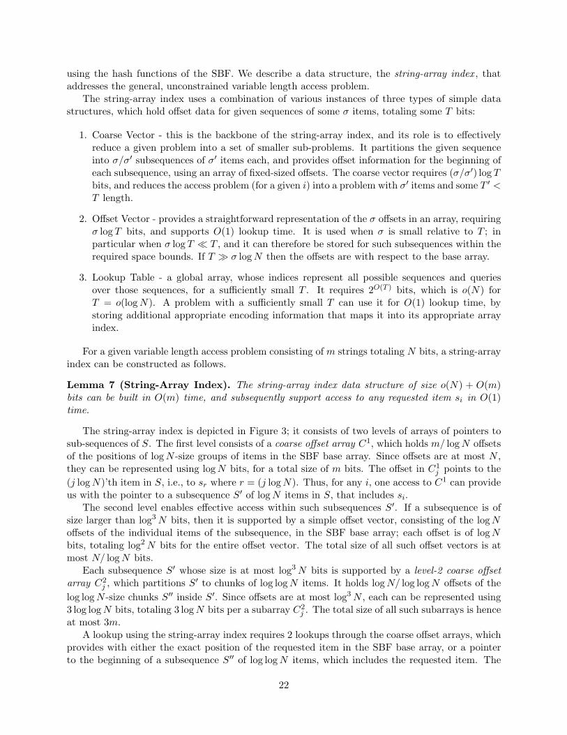
The string-array index uses a combination of various instances of three types of simple datastructures, which hold offset data for given sequences of some σ items, totaling some T bits:

1. Coarse Vector - this is the backbone of the string-array index, and its role is to effectivelyreduce a given problem into a set of smaller sub-problems. It partitions the given sequenceinto σ/σ′ subsequences of σ′ items each, and provides offset information for the beginning ofeach subsequence, using an array of fixed-sized offsets. The coarse vector requires (σ/σ′) log Tbits, and reduces the access problem (for a given i) into a problem with σ′ items and some T ′ <T length.

2. Offset Vector - provides a straightforward representation of the σ offsets in an array, requiringσ log T bits, and supports O(1) lookup time. It is used when σ is small relative to T ; inparticular when σ log T ¿ T , and it can therefore be stored for such subsequences within therequired space bounds. If T À σ log N then the offsets are with respect to the base array.

3. Lookup Table - a global array, whose indices represent all possible sequences and queriesover those sequences, for a sufficiently small T . It requires 2O(T ) bits, which is o(N) forT = o(log N). A problem with a sufficiently small T can use it for O(1) lookup time, bystoring additional appropriate encoding information that maps it into its appropriate arrayindex.

For a given variable length access problem consisting of m strings totaling N bits, a string-arrayindex can be constructed as follows.

Lemma 7 (String-Array Index). The string-array index data structure of size o(N) + O(m)bits can be built in O(m) time, and subsequently support access to any requested item si in O(1)time.

The string-array index is depicted in Figure 3; it consists of two levels of arrays of pointers tosub-sequences of S. The first level consists of a coarse offset array C1, which holds m/ log N offsetsof the positions of log N -size groups of items in the SBF base array. Since offsets are at most N ,they can be represented using log N bits, for a total size of m bits. The offset in C1

j points to the(j log N)’th item in S, i.e., to sr where r = (j log N). Thus, for any i, one access to C1 can provideus with the pointer to a subsequence S′ of log N items in S, that includes si.

The second level enables effective access within such subsequences S′. If a subsequence is ofsize larger than log3 N bits, then it is supported by a simple offset vector, consisting of the log Noffsets of the individual items of the subsequence, in the SBF base array; each offset is of logNbits, totaling log2 N bits for the entire offset vector. The total size of all such offset vectors is atmost N/ log N bits.

Each subsequence S′ whose size is at most log3 N bits is supported by a level-2 coarse offsetarray C2

j , which partitions S′ to chunks of log log N items. It holds log N/ log log N offsets of thelog log N -size chunks S′′ inside S′. Since offsets are at most log3 N , each can be represented using3 log log N bits, totaling 3 log N bits per a subarray C2

j . The total size of all such subarrays is henceat most 3m.

A lookup using the string-array index requires 2 lookups through the coarse offset arrays, whichprovides with either the exact position of the requested item in the SBF base array, or a pointerto the beginning of a subsequence S′′ of log log N items, which includes the requested item. The

22

� ������ ��� �

� ����� ��������� � ���� "!$#&% ' (*),+.-

/ 0 1 2

3 4�57698;:=<*>@?A B�C�D�E�F G HJI"K�L;MN O P;Q,R.SUT

V W X Y

Z\[^]._�`bac dfehgji

Figure 3: The String-Array Index data structure.

items within each subsequence S′′ are accessed either through an offset vector built for S′′, or usinga global lookup table shared by all subsequences, depending on the size of S′′. We use a thresholdT0 = (log log N)3, to determine which method is used. Let S′′ be of size T = T (S′′) bits.

If T > T0, we keep for S′′ an offset vector; since T ≤ log3 N , each offset can be representedusing 3 log log N bits, and the offset vector for S′′ will consist of such log log N offsets, totaling size3(log log N)2 ¿ T (S′′). Hence, the total size of all such offset vectors is o(N).

It remains to deal with S′′ such that T ≤ T0. We keep a single global lookup table, thatwill serve all such sub-problems. An entry to the lookup table consists of a string representing asubsequence S′′ and an index i, 1 ≤ i ≤ log log N . For each such entry, the lookup table will returnthe offset from the beginning of S′′ in the SBF base array, of the i’th item in S′′.

The lookup table consists of a simple array LT , whose indices represent all binary combina-tions representing the entries 〈L(S′′), i〉, where L(S′′) is a bit sequence which provides a uniquerepresentation of the lengths of items in S′′. Note that since we are only interested in obtaining anoffset within S′′, we need not take into consideration the bit sequence of S′′ itself, thus we need toprecompute only the possible combinations of counter lengths such that the total length of S′′ is≤ T . This reduces the number of keys within the lookup table dramatically. The subarray L(S′′)consists of an encoding of the lengths of the items in S′′, so as to allow unique interpretation of theT -bit subarray representing S′′. The encoding in L(S′′) has the property that the size of each codeword is proportional to the encoding length of the value it represents. This is obtained using, e.g.,Elias Encoding (see Section 4.5). The length of L(S′′) is either O(log log N) or o(T ). In additionto the representation L(S′′), the entry includes the index i (consisting of log log log N bits).

It is easy to see that since T ≤ T0, the total size of LT is o(N) bits, and that all its entries canbe computed in o(N) time. The subarray L(S′′) is stored for each S′′ whose size T is less than T0

as part of the SBF. The offset of the ith item in such S′′ is obtained by looking up at LT the valuecorresponding to the entry consisting of the 〈L(S′′), i〉, as determined using L(S′′).

In summary, the string-array index consists of the following components: the coarse offset arrayC1, an array C2 consisting of all level-2 coarse offset arrays C2

j , the offset vectors of first level andsecond level sequences, the global lookup table LT , and the length arrays L(S′′). The total size

23

of the string-array index is o(N) + O(m), its construction takes O(m) time, and it can be used asdiscussed to solve the variable length access problem in O(1) time. The lemma follows.

Note that when actually implementing a string-array index, several of the structures could beeliminated or altered due to practical considerations. In particular, even for relatively large valuesof N , one should not be concerned with paying O(log log N) factor overhead for a fraction of thedata structure.

The SBF can now be constructed as stated in Theorem 6: the base-array is built in O(N) timeby updating the counters Ci as the input data set items are hashed one by one. Subsequently,building the string-array index over the base array. This requires using during construction timea temporary array of O(m log M) bits. The next subsection shows how to construct the SBFincrementally, as well as how to support update operations, without using any temporary array,and within the storage bounds of N + o(N) + O(m) bits.

4.4 Handling updates

We show how to extend the string-array index data structure described above, to allow dynamicchanges in the data-set, for a base array of an SBF. When one of the counters increases its bit-sizein the base array, additional space needs to be allocated within the base array to accommodatethe enlarged substring. It is also necessary to update the string-array index structure to reflectthe changes made in the base-array. Delete operations only affect individual counters, and do notaffect their positions, and hence the string-array index. To remain within storage bounds, after along sequence of deletions the entire data structure is rebuilt, with amortized constant time perdeletion.

To support inserts, we allocate a slack of extra bits in the base array. In particular, we add εmslack bits, one every 1/ε items, for some ε > 0. A counter which needs to expand “pushes” theitem next to it, which in turn pushes the next item, until a slack is encountered. For each item, thenearest slack is initially allocated within a distance of at most 1/ε items. However, upon expansion,the nearest slack may not be available, in case at least one of the items between the expanded itemand the slack was already expanded. In such case, farther slack will need to be used. The cost ofexpansion is linear in the number of items that need to be pushed, assuming that each item fitsinto machine word.

The next lemma bounds the expected distance from an expanded item to the nearest availableslack, using the fact that items location is determined at random by the hash functions of the SBF.For purpose of simplicity, we assume full randomness. It is assumed that the number of inserts isat most ε′m, for some ε′ > 0. After ε′m inserts, the base array is refreshed by moving counters sothat slacks are again placed in 1/ε intervals, and the string-array index is updated accordingly.

Lemma 8. Suppose that the size of some counter Cj increases, and that the total number ofinsertions is at most ε′m, for ε′ = ε/2e. Then, the number of items between Cj and the firstavailable slack, denoted `j, satisfies E(`j) = O(1/ε).

Proof. Suppose first that Cj increases for the first time. A slack is available within the sub-arrayof i/ε items following Cj , if the number di of expansions of items within this sub-array is less thani. Since items are hashed into the base array at random, then for any sequence of ε′m insertions,di is bounded by a binomial with parameters (ε′m, i/(εm)). Hence, E(di) ≤ iε′m/(εm) = iε′/ε.The probability that items within i chunks will need to move upon an insertion is bounded byPi = Pr(di ≥ i) = Pr(di ≥ ε

ε′E(di)) ≤ (e ε′ε )i, with the last inequality due to Chernoff bounds.

Hence, E(`j) ≤∑∞

i=1 i/ε · Pi ≤∑∞

i=1(i/ε) · (e ε′ε )i = 1/ε

∑∞i=1 i(1

2)i ≤ 2/ε.

24

It remains to account for repeated expansions of particular counters. Suppose that a counter Cj

has a sequence of x expansions. For the last expansion, it is guaranteed that the nearest x−1 slackbits are not available. Further, items within the nearest x − 1 chunks of size 1/ε might also havebeen expanded resulting with additional slack unavailability. On the other hand, the additionalexpected cost can be amortized against the 2x updates to Cj which are required to facilitate xexpansions. The expected amortized cost per repeated expansion remains O(1).

The string-array index is updated when items are moved. The update of the structure hasthe same computational complexity as that of updating the base array itself, since essentially onlyoffset information about items that are pushed needs to be changed in the string-array index. Theexpected amortized cost per update therefore remains O(1). Since refreshing the entire base arrayand updating the string-array index takes O(m) time, the amortized cost of such refresh and updateis O(1/ε′) per update.

4.5 An alternative approach

The data structure can be made more compact, while sacrificing lookup performance, by usingthe C1 and C2 indexes and not building any further structures. Once the problem is reduced tolog log N items, we allow a serial scan of the sub-group in order to access the requested item. Toallow that, we need a compact prefix-free encoding that can be read sequentially. For this purposewe use a combination of Elias encoding and a method which is more compact for small counters.

In this scenario, a sub-group consists of log log N items. Using the encodings presented in thissection, each counter with value c can be encoded with close to log c bits. Therefore, this approachrequires N bits to encode the actual counters in the original vector, with additional o(m) bits forthe structures of C1 and C2, while on average a lookup costs log log N . The same approach that isdescribed in Section 4.4 can be used to allow dynamic maintenance of the structure.

Elias encoding

The Elias encoding [Eli75] consists of the following method: Let B(n) be the binary representationof the integer, with length L(n). A binary prefix code B1(n) is created by adding a prefix of L(n)−1zeroes to the beginning of B(n). Now we create the sequence representing n by encoding B1(L(n))followed by B(n) with its leading 1 removed1. The total length of this representation is

L2(n) = blog2 nc+ 2blog2 (blog2 nc+ 1)c+ 1

The steps method

Elias encoding is a strong and simple method to create an encoding which is prefix-free while beingcompact. However, for very small numbers the overhead of log log n bits and the constants thatare involved is substantial and should be avoided. For example, to encode the number 1 (actuallyencoding the number 2) we need 4 bits. In many data-sets, most counters will be 1, so for anoptimal hit ratio of 0.5, the average is 2.5 bits per counter.

To solve that problem, we use a Huffman-like compact encoding for small numbers. For example,using 0 to represent 0, 10 to represent 1 and 11 means the number is bigger than 1, with the Eliasencoding of this number following the prefix. This reduces the cost to 1.5 bits per counter, fordata-sets as described above. It is further reduced if we encode longer sequences, reducing theoverhead to an ε as small as we choose. Full details are omitted due to space limitations).

1The Elias encoding does not encode the number 0. Therefore, when encoding n, we actually encode n + 1, thisdoes not effectively change the size expectations

25

4.6 Storage requirements improvement

The storage bounds presented in Theorem 6 should be competitive with current known solutionto the variable length access problem, presented in Section 4.2. In this section we will propose animprovement to the string-array index structure which reduces its storage requirements and makesit competitive with those methods.

4.6.1 String-array index memory reduction

The key notion that enables the reduction in the memory requirements is that the number of offsetsin each offset vector can actually be reduced to create a smaller offset vector. Our goal is to producea string-array index which, for a bit-array of N bits, requires additional O(N/ log log N) bits ofstorage. To reach this goal, we will reduce each and every substructure of the string-array indexto within the required space. The following theorem states this formally, and the modificationsneeded in the string-array index are described in its proof.

Theorem 9. The string-array index structure for a bit array of N bits, supporting lookups in O(1)time and insertions,deletions and updates in O(1) expected amortized time, can be implementedusing o(N/(log log N)c) + O(m/(log log N)c) bits, for any given c ≥ 0.

Proof. The following description does not change the structure of the string-array index. The basicbuilding-stones and the structure of the layers are the same, with changes only in the constants andthresholds used in the construction of the data structure. The remainder of this proof describes thechanges made in each of the layers of the string-array index, starting with the first level of coarseoffset vectors (C1), and ending with the lookup table.

In C1, each offset is of log N bits. Instead of holding m/ log N such offsets, allocate onlym/(log N)1+c such offsets, resulting in a total storage of m/(log N)c bits for C1. As a result, C1

divides the bit-array into subgroups of size (log N)1+c items.The size of a complete offset vector for such subgroup S′ of size T bits is (log N)1+c log T bits.

Therefore, S′ will have a complete offset vector in C2 if it satisfies T/(log log N)c > (log N)1+c log T .This is necessary to ensure that the string-array index is smaller by a factor of (log log N)c thanthe original vector. From this we can derive the constrain on T :

T/ log T > (log N)1+c(log log N)c

To find a minimal value for T from this, we use the following claim (all usage of log x in this claimrefers to log2 x):

Claim 10. The inequality T/ log T > β is satisfied for T > 3β log β and β > 3

Proof. Let T ′ = 3β log β ⇒ log T ′ = log 3 + log β + log log β.

β log T ′ = β(log 3 + log β + log log β) < 3β log β = T ′

The last inequality is correct for β > 3. Since the claim is true for T ′, and the expression T/ log Tis increasing with T , the claim follows for T > T ′.

To satisfy the above inequality, we require that T satisfies the looser bound:

T/ log T > (log N)1+c(log N)c = (log N)1+2c

26

From Claim 10, this is satisfied when

T > T ′0 = 3(1 + 2c)(log N)1+2c log log N

and therefore satisfied when T ′0 = (3+6c)(log N)2+2c. Notice, however, that this inequality actuallyallows for the offset vector to be smaller than the original vector by a factor of (logN)c. Whencalculating the bound with the original value of β = (log N)1+c(log log N)c, this bound can bereduced to T > T ′0 = (3 + 6c)(log N)1+c(log log N)1+c.

Subsequences which are smaller than (3 + 6c)(log N)2+2c bits are treated with a coarse offsetvector in C2. The size of each offset is

log ((3 + 6c)(log N)2+2c) = log (3 + 6c) + (2 + 2c) log log N

In the second level, each subgroup will be divided into subgroups of (log log N)1+c items, generatingcoarse offset vectors of total size O(m/(log log N)c) bits.

The last part of the structure is the third level, consisting of offset vectors and lookup table.Each subgroup in this level consists of (log log N)1+c items. Similarly to the calculation shownabove, we set a constraint at

T/(log log N)c > (log log N)1+c log T ⇒ T/ log T > (log log N)1+2c

By Claim 10 it produces the limit T ′′0 = (3+6c)(log log N)2+2c. Subsequences larger than this limitwill use an offset vector, and smaller than it will use the lookup table, which needs to support bitsequences of maximal size T ′′0 . The table consists of (log log N)1+c · 2T ′′0 entries, each of size log T ′′0bits. This calculation is asymptotically smaller than N/(log log N)c for large enough values of N ,meaning we can store the lookup table in o(N/(log log N)c) bits, as required.

This completes the modifications needed to reduce the storage requirements of the string-arrayindex. Given the reduced storage, it is competitive with the various solutions given to the variablelength index problem, supporting lookup in O(1) time and update in amortized O(1) time.

4.7 Implementation issues

During the implementation of the string-array index, the emphasis was on providing the fastestand most efficient implementation available. The implementation also needed to address severalissues, and several optimization schemes were thought of during that phase. In this section we givea survey of those issues.

4.7.1 Memory management

Within the string-array index, there is usage of blocks of allocated memory, for the original countervector, the various offset vectors and the lookup table. A simple implementation allocates spacefor each and every such memory block individually, using the memory allocation scheme of thegiven compiler. This method often creates fragmented memory area, in which the memory is notallocated as one continuous block, but is spread across the available memory.

One of the popular uses of Bloom Filters is in distributed systems, where the filter is often sentfrom one node to another as a message. By creating fragmented memory area, it is impossible tosend the string-array index as-is without preparing it to be sent and packing it as a message. Thisaction is possible, but incurs computation overhead when preparing to send the string-array index,and also when receiving it. The goal is to create the data structure as one continuous block andwhen it is needed to be sent, simply transmit the contents of the memory block that includes all

27

the information needed to fully reproduce the string-array index. In the remainder of this sectionwe present the methods needed to facilitate such an implementation, and present the challengesand their algorithmic solutions.

The following description explains the implementation details for each layer of the string-arrayindex structure, and the overheads involved (if any). It starts with the top levels, namely thecounters array and the first level coarse offset vectors, and continues to drill through the structure,ending with the third level of offset vectors, and the lookup table.

Raw counters array and coarse offsets level 1 The first levels of the structure are rathereasy to implement in a continuous fashion. The raw counter array itself is inherently a sequence ofbits, and needs no further adjusting. The first level coarse offset vector can be places immediatelyafter the raw vector, which requires that we record the size (in bits) of the raw vector - an overheadof log log N bits which we can allow.

In order to fully represent an offset vector (coarse or complete), we need to know two detailsabout it: first, we must know if it is coarse or not. We need not know the actual number of offsetswithin it, since this number is implied from the string-array index structure. Second, we need toknow the size of the offsets, in order to allow a direct access to any offset within the offset vector.In the case of the first level coarse offset vector (C1), we know for sure that it is coarse, and that itcontains m/ log N fixed-size offsets of log N bits each. Since we know N (we kept it previously, toallow access to the beginning of C1), we can store C1 as a continuous bit-array which contains theinformation of all the offsets in their binary form, where each offset inhabits log N bits. To accessC1

i , we need to access the (i log N)th bit from the beginning of C1, and read the next log N bits,which contain the actual offset.

Level 2 offset vectors Second level offset vectors (C2) are a far more complex challenge. Theseoffset vectors differ in their size, since they point at subsequences of varying lengths, which trans-lated to different sizes of offsets. Furthermore, some of these offset vectors are coarse (pointing atshort subsequences) and others are complete offset vectors. The required information for an offsetvector C2

j can be gathered from C1: by sequentially reading the offsets of the jth and the (j + 1)stgroup, we can calculate the size of the subsequence and decide if the offset vector is coarse or not,and what is the size of each offset. Assuming that we store all the C2 vectors in a continuous bitarray, we still need to know exactly where in this bit-array the jth offset vector begins.

This problem is in fact another instance of the variable length access problem. It is an appealingidea to solve it by using a string-array index in a recursive fashion. However, this problem can besolved with an acceptable overhead by simply holding an offset vector which points to the bit-arrayrepresenting C2. The total size of C2, as shown above, is bounded by N/ log N + 3m bits. It isdivided into m/ log N offset vectors, so an offset vector for C2 will hold m/ log N offsets, each of sizelog (N/ log N + 3m) ≈ log N bits. This accumulates to an additional size size of approximately mbits. Accessing the correct offset vector is simple: the information regarding its size and coarsenesscan be obtained from C1 as described. Its starting point within C2 is read from the offset vector,where a single lookup (and reading of N/ log N + 3m bits) provide the offset. For additional spacesavings, the size of the C2 bit-array can be kept (requiring approximately log N bits), and all offsetsthat point at C2 will be limited in size to |C2|.

Level 3 offset vectors and lookup table Level 3 of the string-array index is similar to thesecond level, with the additional complexity of the lookup table. The lookup table itself can beomitted when transmitting the string-array index, because it is dependant only on the parameters

28

of the string-array index and can be generated in the receiving node. Otherwise it can be easilykept as a bit-array with simple lookup into it. The level 3 offset vectors are kept in a bit-array,where each offset vector accommodates a constant size. The size needed for such an offset-vectoris 3(log log N)2 bits. However, to remain within the stated storage bounds, we cannot allocate thisamount of storage to each and every subgroup. We must skip the subgroups handled by the lookuptable when encoding this bit-array.

To solve this problem, we encode in the bit-array only those offset vectors which actually arein use. In this case, when looking for the jth offset vector, we need to translate it to rj ≤ j, whichis actually the index of the same subgroup in the collection that includes only those subgroupshandled by offset vectors. We create a bit-vector F of size m/ log log N bits, with the ith bit beinga flag marking whether the ith subgroup is handled by an offset vector. Given this bit-array, wecan calculate rj by using the rank operator, rj = rank(F, j)2. Calculation of the rank operator fora bit-vector of N bits is possible using o(N) bits in O(1) time [Jac89, Mun96], so using additionalm/ log log N bits of storage we can perform the needed translation.

Summary This section outlined the method for storing the entire string-array index in a con-tinuous fragment of memory, while still allowing random access to any given element. To facilitatethis improvement, additional log log N + m + m/ log log N bits of storage are needed.

4.7.2 Offset vectors division

The offset vectors of C1 and C2 are divided by their size to coarse offset vectors and completeoffset vectors. The division is necessary for space limitations, when holding a complete offsetvector requires too much space, we are forced to use a coarse offset vector. However, there may besituations in which a single subgroup is so large that it can compensate for the small size of othersmaller groups, such that groups that individually would not merit a complete offset vector maybe handled by one.

The advantages of this approach are clear: when using a complete offset vector instead ofa coarse one, we reduce the number of internal lookups needed for a single item lookup. Also,a subgroup that is handled by a complete offset vector does not need further processing in thefollowing levels of the string-array index and therefore is more space efficient.

The algorithm for producing this optimization is rather simple: let I be the number of itemswithin each subgroup, and T i be the total size in bits of subgroup i. The condition for keepinga complete offset vector is I log T i < T i, meaning that the size of the complete offset vector isstill smaller than the size of the original group (we might, of course, be using a tighter threshold,requiring that the offset vector is substantially smaller than the original size of the group). Thealgorithm will collect a group of subgroups G, according to a given selection criterion, and keepbuilding complete offset vectors as long as

∑i∈G I log T i <

∑i∈G T i. The selection criterion might

be as simple as adding the following groups in consecutive order, or more complex, such as at-tempting to create an optimal packing of the groups, such that as little groups as possible are leftwithout a complete offset vector.

This optimization is very useful in situations where the data is highly skewed. In these cases,the data is usually dominated by a small number of frequent items, with a large number of relativelyrare items. This will result in a small number of subgroups whose binary encoding is rather large,and those groups can encompass within them a large number of smaller groups. As the data tends

2rank(V, j) returns the number of 1 bits occurring before and including the jth bit in the bit vector V.

29

to be more uniform (with skew ≈ 0), this strategy loses some of its strength, but still provides animprovement.

5 Applications

In this section we explore a range of applications that may take advantage of the SBF. The firstcategory of such applications consists of extensions to methods or abilities of the regular BloomFilter. For example the Bloomjoins method, which allows for efficient joins within a distributeddatabase, is improved be the usage of SBF within it, transforming it to Spectral Bloomjoins. Newqueries can be answered while still maintaining efficiency and accuracy.

The second category has new applications which use the SBF to efficiently perform tasks whichweren’t possible with a simple Bloom filter. One example of such task is ad-hoc iceberg queries,in which one is interested in a small subset of the most frequent items within a data-set. Theseitems can be thought of as the “tip of the iceberg”, where we ignore the majority of the items inthe data-set which lie beneath the surface. The SBF allows us to perform ad-hoc iceberg queries,in which the threshold determining the size of the result-set is set only at query time, improvingon current methods which require a given threshold to perform preprocessing of the data.

5.1 Aggregate queries over specified items

Spectral Bloom Filters hold mostly accurate information over each and every item of the data set.Therefore it can approximately answer any (aggregate) query regarding a given subset of the items,so that the error ratio is expected to be ESBF , and the size of the error is expected to be smallerthan the average frequency of items in the set, f . An example for such query is:

SELECT count(a1) FROM R WHERE a1 = v

In performing this query, the SBF acts as an aggregate index built upon the attribute a1 andproviding the (mostly) accurate frequency of v in the relation. Other aggregates, such as average,sum, max etc. can be easily implemented using this basic ability. The SBF behaves very much likea histogram where each item has its own bucket. Since the SBF keeps the full information, it isvery versatile in its uses, while requiring storage proportional to the size of the set.

5.2 Ad-hoc iceberg queries

In many situations, a data-set is tracked regularly in the lookout for items which are more frequentthan a certain threshold. It is desirable to set triggers that will alert us once an item with a highcount is encountered. For example, a company which tracks customer calls can create a calculationthat reports their likeliness to churn. Once a customer with a high churning probability contactsthe company, the company representative should be alerted, so he can offer him special deals. Thethreshold for such special treatment is dynamic, and depends on many factors, so the calculationcannot be executed a priori. Queries of this kind are often referred to as “iceberg queries”, sincethey deal with a small fraction of the data, while the main body of the data-set remains hiddenunderneath the surface.

The example described above presents an ad-hoc iceberg query, in which the threshold againstwhich items are tested upon insertion is dynamic and possibly changes between queries. Methodsto handle iceberg queries, proposed in [FSGM+98, MM02] require a certain preprocessing the datagiven a static threshold. When the threshold changes, the methods of [FSGM+98, MM02] require

30

rescanning of the data using the new threshold (or in the case of streaming data [MM02], it cannotbe done), while the SBF does not require any additional scan of the data, other than one thatexamines the data against the counts stored in the SBF.

Traditional methods for iceberg queries

Iceberg Queries [FSGM+98] are queries of the form

SELECT t1,t2, . . . ,tk,count(rest) FROM RGROUP BY t1,t2, . . . ,tk HAVING count(rest) >= T

Usual database execution methods are not efficient for such queries, since they usually requiresorting of the entire relation and then performing the reduction. If the threshold T is such thatonly a small part of the relation is returned by the query, then the execution plan is far fromefficient. Another version of iceberg queries is dealt with in [EV02], where iceberg techniques arerequired to perform over streaming data. The solutions presented in [FSGM+98, EV02] are bothconstrained in the sense that they require a prior knowledge of T to function, and they do notmaintain complete knowledge of the data set. This optimization allows for very compact memorystructures, but prevents the usage of the algorithms in ad-hoc situations, where the threshold mightchange during inspection.

Suppose, for example, that a query is executed with a threshold of 1%, which turns out to betoo high and the query returns with no results. To lower the threshold and execute the query again,the data must be fully scanned again and the data structure needs to be built again. Since the datastructures are very compact and assume that many items hash to every bucket, the informationstored has a very high error ratio, so it can hardly be used for exact queries, trying to figure out theitems which comply to the new threshold. To prevent this from happening, an initial low thresholdmust be selected, but this neutralizes many of the the advantages of the proposed algorithms,requiring them to use a lot of memory (or forcing a high error ratio on the results).

In this section we present two ways to utilize SBFs in ad-hoc iceberg queries: a straight for-ward implementation, using a regular SBF to answer the queries, and a method similar to theMULTISCAN-SHARED method of [FSGM+98], performing progressive filtering of the data.

Algorithm & Error Analysis for Iceberg Queries

The SBF can be used as-is for purposes of iceberg queries answering. For streaming data, theSBF can be built while the data flows, and any item whose frequency passes the given thresholdis reported. For non-streaming data hashed into an SBF, a single scan of the data is performed.Each item inserted is checked within the SBF for its frequency, if it exceeds the threshold, the itemis reported. The threshold can be dynamic and determined at query time, and not while hashingthe data.

Using an SBF to handle iceberg queries might generate errors due to its probabilistic nature.These errors can be eliminated by performing a scan of the potentially heavy itemset to retrievethe actual counts of each item from the range of items R, as in [FSGM+98]. This is not possibleunder the assumption of streaming data unless some additional data structures are built to supportthe extra queries. In the remainder of this section, no such scan is assumed.

The SBF may produce false-positives. That is, all items that should be reported are indeedreported, along with several items which do not pass the threshold. If we denote by Q the set ofall items returned by our algorithm, and for an item t, we denote by ft its true frequency in R,

31

it is guaranteed that ∀t ∈ R s.t. ft ≥ T, t ∈ Q. However, Q might include some items for whichft < T . Notice that for iceberg queries purposes, the error is only a subset of the usual BloomError, because the errors have to be big enough to pass the threshold.

Assume that the distribution of item frequencies in R behaves according to some function d(f),such that for a frequency f ′, d(f ′) represents the ratio of items in R with that frequency. Forexample, for uniform data d(f) will be a constant. We denote by n the number of distinct itemsin R.

Note that since we are answering a boolean query (is the item over the threshold or not), foritems with frequency greater than T , we care not whether there was a bloom error or not, sinceit does not affect the outcome. We consider items whose frequency is f ′ < T . There are nd(f ′)items with frequency f ′. For an item in that group to belong to the output set Q it must bestepped over by k items of frequency larger than T − f ′. This is approximately equal to the BloomError generated by hashing only the items with big enough frequencies (we ignore secondary errorsgenerated by two items mapped to the same bit and so on). We denote by Df ′ = n

∑∞i=T−f ′ d(i)

the number of items with such frequencies, so for each f ′, the actual error rate in this scheme is

Ef ′ ≈(1− e−kDf ′/m

)k, using the same calculation given in Section 2.1. Thus, the total error rate

across all items is

E =T−1∑

f=0

d(f)Ef ≈T−1∑

f=0

d(f)(1− e−kn/m

P∞i=T−f d(i)

)k

This function represents a tradeoff: for the same parameters, as T increases there are more itemsbelow the threshold, but there are less items big enough to make them pass the threshold. Infigure 4 we present the error rates for Zipfian distribution with several skews and several T s inquestion, in which the tradeoff is obvious. For all except uniform distribution (skew 0), the errorrate increases for very small T , and then it reaches a maximum and drop as T continues to increase,the maximum moves to lower T as the skew increases. The parameters used were k = 5, γ = 1,which represent a smaller Bloom Filter than the optimal. The theoretical Bloom Error for theseparameters is Eb = 0.1, while in the iceberg scenario, the expected error never exceeds 0.025, whileat most relevant thresholds it drops below 0.01.

Multiscan SBF method

Another method of performing iceberg queries is using SBFs in a way similar to the MULTISCAN-SHARED method, as described in [FSGM+98], using several scans of the data. The idea is toperform several stages of filtering, an item passes the combined filter only if it hashes to heavybuckets in all the stages. By building this filter incrementally, we assume that the first filter willfilter out a fraction of the items. Therefore, the second filter will have to deal with less items andthus can be smaller. We propose using SBFs for the various stages, and using the parameters ofthe SBF (namely m and k) to control the strength of the filter. In this implementation, knowledgeof the threshold is required while building the SBF, and it limits the options for ad-hoc queries.

To be competitive with the methods proposed in [FSGM+98], the SBFs need to be of very smallsizes, around 1% of n. This transforms the implementation to Lossy Bloom Filter, since we assumein advance that each bucket will have many items hashing to it, with the Bloom Error reachingprobability of 100%. Notice that if the first filter fails to filter out items, the next filters (whichare smaller) have a very small probability to filter items out. We can determine the properties ofthe next filter on the fly, relying on the performance of the current filter. For example, we cancalculate the average count over the buckets of the current SBF, and if it exceeds the threshold we

32

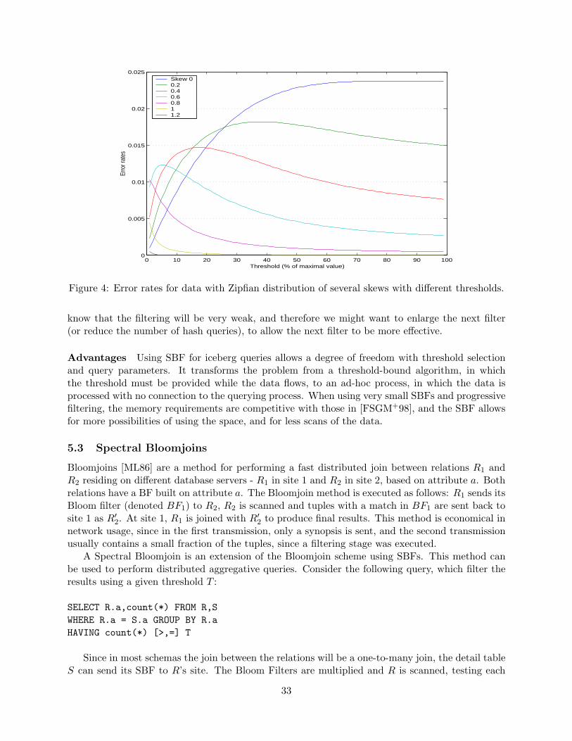
0 10 20 30 40 50 60 70 80 90 1000

0.005

0.01

0.015

0.02

0.025

Threshold (% of maximal value)

Erro

r rat

es

Skew 00.2 0.4 0.6 0.8 1 1.2

Figure 4: Error rates for data with Zipfian distribution of several skews with different thresholds.

know that the filtering will be very weak, and therefore we might want to enlarge the next filter(or reduce the number of hash queries), to allow the next filter to be more effective.

Advantages Using SBF for iceberg queries allows a degree of freedom with threshold selectionand query parameters. It transforms the problem from a threshold-bound algorithm, in whichthe threshold must be provided while the data flows, to an ad-hoc process, in which the data isprocessed with no connection to the querying process. When using very small SBFs and progressivefiltering, the memory requirements are competitive with those in [FSGM+98], and the SBF allowsfor more possibilities of using the space, and for less scans of the data.

5.3 Spectral Bloomjoins

Bloomjoins [ML86] are a method for performing a fast distributed join between relations R1 andR2 residing on different database servers - R1 in site 1 and R2 in site 2, based on attribute a. Bothrelations have a BF built on attribute a. The Bloomjoin method is executed as follows: R1 sends itsBloom filter (denoted BF1) to R2, R2 is scanned and tuples with a match in BF1 are sent back tosite 1 as R′

2. At site 1, R1 is joined with R′2 to produce final results. This method is economical in

network usage, since in the first transmission, only a synopsis is sent, and the second transmissionusually contains a small fraction of the tuples, since a filtering stage was executed.

A Spectral Bloomjoin is an extension of the Bloomjoin scheme using SBFs. This method canbe used to perform distributed aggregative queries. Consider the following query, which filter theresults using a given threshold T :

SELECT R.a,count(*) FROM R,SWHERE R.a = S.a GROUP BY R.aHAVING count(*) [>,=] T

Since in most schemas the join between the relations will be a one-to-many join, the detail tableS can send its SBF to R’s site. The Bloom Filters are multiplied and R is scanned, testing each

33

tuple in SBFRS against the threshold T . Results can be reported immediately since no value isrepeated more than once in R. When using “>” (or “≥”) as the filter operator, there is only asmall fraction ρ of false positive errors, E(ρ) = ESBF , and no false negatives. Since the errors areone-sided, they can be eliminated by retrieving the accurate frequencies for the items in the resultset, resulting in a fraction of ρ extra accesses to the data. The effectiveness of this method increasesas the size of the result set decreases. When using the “=” operator, two-sided errors are possible,with recall of 1− ESBF , and possibly additional false-alarms.

The SBF’s capability to represent multiplicities can also be used in queries which perform nofiltering, such as the following:

SELECT R.a,count(*) FROM R,SWHERE R.a = S.a GROUP BY R.a

To perform this query using a Bloomjoin, the full scheme described in [ML86] must be exe-cuted, with Bloom Filters and tuple stream sent back and forth between the sites. However, usingSBF multiplication, a shorter scheme can be executed, assuming that both S and R have a SBFrepresenting the attribute a present, and R being the primary query site: S sends its SBF (SBFS)to R’s site, where SBFS and SBFR are multiplied to create SBFSR. Next, R is scanned, and eachtuple is checked against SBFSR for existence. If it exists, the item and its frequency are reported.

This scheme does not guarantee exact results. Items which appear in R and not in S maybe reported because of errors in SBFS . The error ratio expected is the standard Bloom error,as described in Section 2.1. Also, the frequencies reported are subject to Bloom Error and maybe higher than their actual value. The size of these errors can be estimated using the calculationdescribed in Section 2.3, or improved by using the Minimal Increase method (when no deletionsare necessary). To ensure the uniqueness of items in the results, we suggest the use of a validatingSBF for that purpose. This method saves the transmission of data back to the main site. If themain site has to be the one reporting the results, the final answer may be sent back to it, withminuscule network usage.

Advantages Using SBF for Bloomjoins simplifies and shortens the algorithm for performingdistributed joins, by allowing the query to be answered after transmitting one synopsis from site tosite, eliminating the need for a feedback. While the SBF itself is slightly larger than a Bloom Filterof the same parameters, this is balanced by the shorter operation scheme, requiring less SBFs tobe sent between sites, and therefore saving bandwidth.

5.4 Bifocal sampling

A Spectral Bloom Filter can be plugged into various schemes that require an index on a relationfor count queries. One such application is Bifocal Sampling [GGMS96], where using an SBF onecan get similar join estimations without using an expensive index. The paper deals with joiningtwo relations with unknown properties by dividing each relation to two distinct groups: dense andsparse tuples. The join size is estimated by combining the groups in all ways possible, creating adense-dense join and sparse-any joins. In the sparse-any case, a join of type t-index [HNSS93] isused, meaning for each tuple in a sample of one relation, a query on the other relation is performedto determine the frequency of the join attribute in the second relation. We sketch the modificationsmade in the bifocal sampling, with reference to the algorithm described in [GGMS96]. By replacingthe t-index with an SBF, the multiplicities used for estimation are replaced by their approximations,resulting with only a small additional error to the overall estimate.

34

When using SBF in this procedure, each error will be multiplied by n/m2. We might also labelitems as dense when in fact they are sparse. For this to happen, multR(v) needs to be smaller thann/m2 and the error rate needs to be big enough to make multR(v) ≥ n/m2. In fact, this kind oferrors might balance the first type of errors.

By following the logic of Lemma 3.3 in the original paper, we substitute multR(v) by mult′R(v),which is the result of querying the SBF for the item v. For tuples that are dense in R, we are certainthat E(τ) = 0. For tuples that are not dense, if mult′R(v) < n/m2 (no Bloom Error or a small one),we have E(E(τ)) = mult′R(v) ≤ multR(v) + γ. From this we need to subtract the tuples which aresparse but considered dense due to Bloom Error. These tuples are rare, since they must be subjectto Bloom Error and also be sparse, but with sufficiently high multiplicity so that when adding theerror, they pass the threshold and become dense. It follows that As ≤ E(As) ≤ As(1 + γ), asrequired.

This deviation in the estimated total will usually be much smaller, and can be very small ifusing the MI method. However, the error can be incorporated into the calculations in the procedureand the estimation can be adjusted according to the expected average error.

Advantages The SBF provides an efficient approximation to the t-index scheme, and enables amore space-efficient implementation of Bifocal Sampling.

5.5 Range queries

Range queries are queries concerning a subset of the relation in which certain attribute is within a(open or closed) range (L,U), for example the following query

SELECT count(a) FROM RWHERE a>L AND a<U

The SBF can provide (mostly) exact information per specific item, but due to its structure hasno support for range queries. When answering such a query, an exhaustive search over the entirerange is not always possible, and is dependent on the size of the range, which can be very expensivewhen the data is sparse in that range or when the range is very large.

Range Tree Hashing In order to accomplish range queries capabilities, we hash both the specificitems in the relation and new items that each represent a range. The ranges are kept in a hierarchy,each range is the union of the ranges represented by its descendants.

Theorem 11. For an attribute in the range R = (L, U) with |R| = r , range queries can besupported with insertion and deletion complexity of log r and constant lookup complexity for distinctqueries. For lookup queries over a range Q ⊆ R, the query requires O(log |Q|) SBF queries.

Proof. We construct a binary tree T , in which every node corresponds to a subrange within R.For each node n ∈ T , we denote its corresponding subrange with Rn, and its sons n1, n2 . . . , nk

correspond to non overlapping subranges of Rn such that Rn1 ∪Rn2 ∪ . . . ∪Rnk= Rn. Each node

is associated with a value vn ∈ V, V ∩ R = ∅. The hash functions of the SBF hash the extendedrange R ∪ {v1, v2 . . . , v|T |}.

When inserting an item v into the SBF, every node n in T with v ∈ Rn (these correspond toa single branch), inserts its value vn into the SBF as well. Since the depth of a tree is log r, everyinsert into the SBF is transformed into log r inserts. The same holds for deletions.

35

� �

� � � �

� � �

� � � ���

�

�

W����� �������! #"�$�%�& ')(+*!,.-�/ 021�3�4!5#687 9�:<;>= ?A@>B C DFE�G H I

Figure 5: A Part of the tree created in order to handle range queries.

When performing lookup of a single value, there is no need to traverse the tree. A direct query isperformed against the SBF and thus a single lookup is required, with the implied SBF complexity.

For this proof we assume the usage of a binary tree, though other trees may be used as well.For ease of reading, we denote log2 n by log n. To query the tree for the range, we perform a BFSover the tree. Once a node n contains a range fully enclosed in Q, we query the SBF for vn, addthe result to our grand total and do not continue to its descendants. If the range of the node doesnot intersect with Q, we do not continue to query its descendants.

We denote by lmin the highest level of the tree in which we performed a query in the SBF. Inthis level, we can perform as many as 2 queries, because if Q includes 3 adjacent nodes in it, atleast two of them belong to the same parent node, and therefore the parent node is fully enclosedin Q, and lmin would not be the minimal level in which a query is performed.

The queries in level lmin remove from Q the middle part, which leaves (in the worst case) twosmaller ranges Ql and Qr for the next level. Both ranges begin precisely in a node boundary, andcannot spread over two or more nodes in this level (otherwise the parent node would have beencovered). This means that in the worst case, both Ql and Qr generate one additional SBF queryin this level. The remainder is directed to the next level, in which the same logic holds, until (inthe worst case) we reach the final level of the tree and have to perform one final distinct query foreach boundary of the range.

To sum up, each level of the tree (starting with lmin) requires up to 2 SBF queries. We considerthe subtree T ′ which encloses the entire range Q. Its height is log |Q|, therefore the entire processrequires up to 2 log |Q| queries.

Note that when using trees with degree of p (rather than binary trees), the lookup complexitychanges to p logp |Q|, and similarly insertion and deletion complexity are reduced to logp r. Theseobservations are directly related to the depth of the tree.

Size considerations The SBF now must contain additional items corresponding to items in therange tree. In the worst case, there are |R| new items (for example, a binary tree whose leaves areranges of size 2, will contain |R|/2 leaves and a total of |R| nodes, each associated with an item in

36

the tree). We denote by S ⊆ R the subset of values appearing in the relation, |S| = n, the numberof distinct items inserted into the SBF. We denote by Va the set of values in the range tree thatactually are inserted into the SBF during the hashing of S. We can state the following claim:

Claim 12. |Va| ≤ n log r

Proof. When inserting any item x for the first time, we insert into the SBF all tree items that liewithin the corresponding tree branch that ends with x. The length of a full tree branch is log r,therefore for n different items we need at most n log r tree items.

By this claim, we require an expanded SBF in order to support the larger domain. This increasesthe memory demands of the SBF to O(N log N) bits. However, this data structure supports a verywide range of queries, both range queries and accurate specific queries in the same data structure.Note also that the structure of the range tree was predefined, while a more elaborate building ofthis tree can provide much better results using a smaller tree.

Discussion Usually, range queries are handled using histograms, which are significantly morespace-economical than the SBF. However, histograms can not guarantee a certain precision fora single query, since extrapolation is needed for ranges which cover parts of buckets, in whichthe distribution of data is normally not known. The SBF guarantees one-sided errors, which isan important property when using the results for decision making. Also, it gives a certain errorguarantee per query, something that histograms cannot produce.

To summarize this section, it may be desirable to use SBF where precision of each and everysingle query and the predictability of errors (both in nature, namely false-positive errors, and size)are the main issues. When memory is the main constraint, the usage of SBF is not the recommendeddecision.

6 Experiments

We have tested the accuracy of the various SBF lookup algorithms described in Sections 2 and3, as well as the space efficiency of the encoding methods described in Section 4.5. Another setof tests examined the string-array index structure, testing both its storage requirements and itsperformance for lookups, updates and initialization.

6.1 Algorithms comparisons

We have tested and compared the three lookup schemes from Sections 2 and 3: Minimum Selection(MS), Recurring Minimum (RM), and Minimal Increase (MI). The SBF was implemented usinghash functions of modulo/multiply type: given a value v, its hash value H(v), 0 ≤ H(v) < m iscomputed by H(v) = dm(αv mod 1)e, where α is taken uniformly at random from [0, 1]. Wemeasured two parameters; the first is the mean squared additive error, which is calculated by

Eadd =

√√√√∑

i∈v

(fi − fi

)2

n

The second is the error ratio Eratio, computed as the fraction of the queries that return erroneousresults. Thus, E(Eratio) = ESBF , and for MS, it is Eb. Each reported result is the average over 5independent experiments with the same parameters.

37

In the first two sets of tests, reported in Figures 6 and 8, we used synthetic data produces bya Zipfian distribution. We used integers as data values, and the data set was constructed of 1000distinct values, with M = 100, 000. We have also conducted experiments in which M , and hencethe average item frequency, was changed, generating smaller (and larger) data sets. The observedbehavior was consistent with the experiments reported here.

In the first set of tests, the skew of the data was changed, from θ = 0 (uniform data) to θ = 2(very skewed data). The results are shown in Figure 8a,b (solid lines). As can be seen, the MIalgorithm has the best performance both in terms of additive error and error ratio, and is verystable with regard to changes in the skew. The RM algorithm outperforms the MS algorithm inboth parameters, but in most cases is no match to the MI algorithm.

In the second set of tests, the storage size m was changed, to result with γ = nk/m ranging fromabout 0.12 to about 2. The results are shown in Figure 6a,b. For a fair comparison between thealgorithms, in this and in all other experiments the RM algorithm used m as an overall storage size;that is the sizes of the primary and the secondary SBFs together being m. This causes the actualγ of the RM algorithm in its primary SBF to be larger than that of the MS and MI algorithms.These experiments show that all three algorithms behave similarly, with RM and MI being almostidentical in their error ratios. The MI algorithm performs best in terms of additive error when mis small (and γ increases). This is due to the fact that it performs a minimal number of actualinsertions into the base array, which becomes critical as the error ratio increases.

The third experiment tested the behavior of the various schemes when the number of hashfunctions (k) changes. The data used was again Zipfian with a skew of 0.5, in all configurations γwas fixed at 0.7 by increasing m along with k. The results are shown in Figure 6c. In the k = 1case, all the methods perform the same (as they should). The MI method improves dramaticallywhen k increases, while the RM method needs k of at least 3 to become effective, with majorimprovement when k increases to 4 and more.

The above experiments show clearly the significant precision and stability of the Minimal In-crease method, and also the substantial improvement that the Recurring Minimum method showsover the Minimum Selection.

In the third set of tests we used real data: the Forest Cover Type database, obtained from theUCI KDD Archive [Arc]. We used the elevation measure as the property indexed by the SBF.The database has a total of 581012 records, with 1978 distinct values for the elevation measure,distributed as shown in Figure 7a. We have tested the performance of the three methods over thisdatabase while changing the value of γ, by changing the size of the SBF. The results, shown inFigure 7b and c, are consistent with the results over synthetic data-sets and display an advantage tothe Minimal Increase and Recurring Minimum methods over the basic Minimum Selection heuristic.The Minimal Increase and Recurring Minimum methods behave similarly throughout this test, witha slight advantage to the Minimal Increase method.

6.2 Deletions and sliding window

Next, we tested the SBFs when faced with deletions. The setup consisted of a series of insertions,followed by a series of deletions and so on. In every deletion phase, 5% of the items were randomlychosen and were entirely deleted from the SBF. The results, shown in Figure 8, compare theerror ratio and the additive error of the SBFs when subject to deletions to their performancewithout deletions. It is evident that the MI algorithm deteriorates dramatically when deletions areperformed. The third graph shows the main reason for that - false-negative errors. Note that almostall of the errors of the MI algorithm are false negatives (MS and RM have no false-negatives). Thismakes it a poor choice when deletions are considered, since the one-sided nature of the errors is no

38

0.2 0.4 0.6 0.8 1 1.2 1.4 1.6 1.8 20

5

10

15

20

25

30

35

40

45

50

Gamma

Addit

ive E

rror

Minimum SelectionRecurring MinimumMinimal Increase

0.2 0.4 0.6 0.8 1 1.2 1.4 1.6 1.8 210

−4

10−3

10−2

10−1

100

Gamma

Erro

r Rat

io (lo

garit

hmic

scale

)

Minimum SelectionRecurring MinimumMinimal Increase

1 2 3 4 5 60

20

40

60

80

100

120

k

Addit

ive E

rror

Minimum SelectionRecurring MinimumMinimal Increase

Figure 6: Accuracy of MS, MI and RM algorithms for various values of γ, with k = 5, with additiveerror (a), and log of error ratio (b), dotted line represent optimal γ. Additive errors in the threealgorithms for various k values, with γ = 0.7 (c). In all experiments, MI and RM are better thanMS, with some advantage to MI.

39

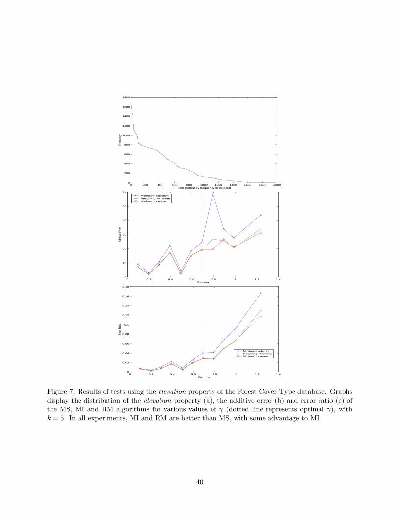
0 200 400 600 800 1000 1200 1400 1600 1800 20000

200

400

600

800

1000

1200

1400

1600

1800

Item (sorted by frequency in dataset)

Freq

uenc

y

0 0.2 0.4 0.6 0.8 1 1.2 1.40

10

20

30

40

50

60

Gamma

Addit

ive E

rror

Minimum selectionRecurring MinimumMinimal Increase

0 0.2 0.4 0.6 0.8 1 1.2 1.40

0.02

0.04

0.06

0.08

0.1

0.12

0.14

0.16

0.18

Gamma

Erro

r Rat

io

Minimum selectionRecurring MinimumMinimal Increase

Figure 7: Results of tests using the elevation property of the Forest Cover Type database. Graphsdisplay the distribution of the elevation property (a), the additive error (b) and error ratio (c) ofthe MS, MI and RM algorithms for various values of γ (dotted line represents optimal γ), withk = 5. In all experiments, MI and RM are better than MS, with some advantage to MI.

40

longer valid.The second test shown in Figure 9, used a sliding window scenario. In this experiment, a total

of M items were inserted, but the SBFs only kept track of the M/5 most recent items as itemswere inserted, with data leaving the window explicitly deleted. The MS and the RM algorithm aremuch better that the MI algorithm for this scenario, with advantage to the RM.

6.3 Encoding methods

We tested the storage needed by the encoding methods described in Section 4.5, comparing theElias method, and several configurations of “steps” for data with varying average frequency ofitems. The results, shown at Figure 10, were compared to the “Log Counters”, which is simply∑m

i=1 log Ci. For data sets with average frequency close to 1 (“almost set”) the steps methodsare more economical, due to their low overhead for small counters. However, the Elias encodingimproves as the average frequency increases, and beats the performance of the steps methods.

6.4 String-array index performance

The string-array index, as described in Section 4.3, needs to be efficient both in its storage require-ments and in the complexity of performing the basic actions needed for the SBF. These actionsare the initial building of the string-array index, increasing a counter, and performing a lookup fora given item. The string-array index was fully implemented in C++, except for the continuousmemory improvement discussed in Section 4.7. We performed several experiments that check thevarious aspects of its usage. Most of these experiments were conducted regardless of our specificusage of the string-array index as a supporting structure for the SBF, but as a stand-alone module.

Performance The performance of the string-array index was tested by populating the structurewith a varying number of items stored in it. For each array size n, we have performed three actions:(i) the structure was initialized with all items being 0, (ii) we performed 10n random insertions ofitems, such that the average frequency at the end of the stage was 10. (iii) Finally we performedlookups for each and every item, totalling at n lookups. We measured the time each of these stagesrequired, dividing the time of stage (ii) by 10, to find the time n insertions needed, in order to createa comparable amount of time. Those tests were executed on a Pentium III (500MHz) machine,with 512MB of RAM.

The results we show are the total times measured, and also the time per action, being simply thetotal time divided by n. The time measured for insertions include the time required for rebuildingthe array, when slacks are exhausted. For each array size we have performed 5 runs of the test, andthe results shown are the average over those runs. Figure 11 shows those two measurements overarray sizes ranging from 1000 to 1 million items. The first set of results show that, as expected,the complexities of those actions are linear with n. These results are in accord with the analyticalresults given in Theorem 6. This is also demonstrated in the second chart, where it is clear that thetime per-action is indeed constant for those actions, even though the time required for insertionshas a large variance. This last observation can be explained by the highly random nature of theinsertions, also note that the average time actually decreases when n increases.

Finally, we compared the performance of the string-array index to a hash table. In order toperform this test, we used the hash table implementation found in LEDA [LED], which uses chainingfor collision resolving. This test compared the full SBF implementation to the hash table, with theSBF using k = 5, and having m equal to the number of buckets allocated in the hash table, and thestraight-forward method for lookup and increase. We also plugged in the same hash functions used

41

0 0.2 0.4 0.6 0.8 1 1.2 1.4 1.6 1.8 20

5

10

15

20

25

30

35

Skew

Addit

ive E

rror

Minimum SelectionRecurring MinimumMinimal Increase MS with deletionsRM with deletionsMI with deletions

0 0.2 0.4 0.6 0.8 1 1.2 1.4 1.6 1.8 210

−2

10−1

100

Skew

log(E

rror R

atio)

Minimum SelectionRecurring MinimumMinimal Increase MS with deletionsRM with deletionsMI with deletions

0 0.2 0.4 0.6 0.8 1 1.2 1.4 1.6 1.8 20.7

0.75

0.8

0.85

0.9

0.95

Skew

False

Neg

ative

s/Tot

al Er

rors

MI with deletions

Figure 8: Performance of MS, RM and MI algorithms for Zipfian distribution with varying skew(θ), with deletions (dotted lines) and without deletions (full lines). Both additive error (top) andlog of error ratio (center) are shown; in all experiments γ = 0.7, k = 5. The third graph showsthe ratio of False Negative errors in the MI algorithm out of the total errors (there are no falsenegatives in MS and RM).

42

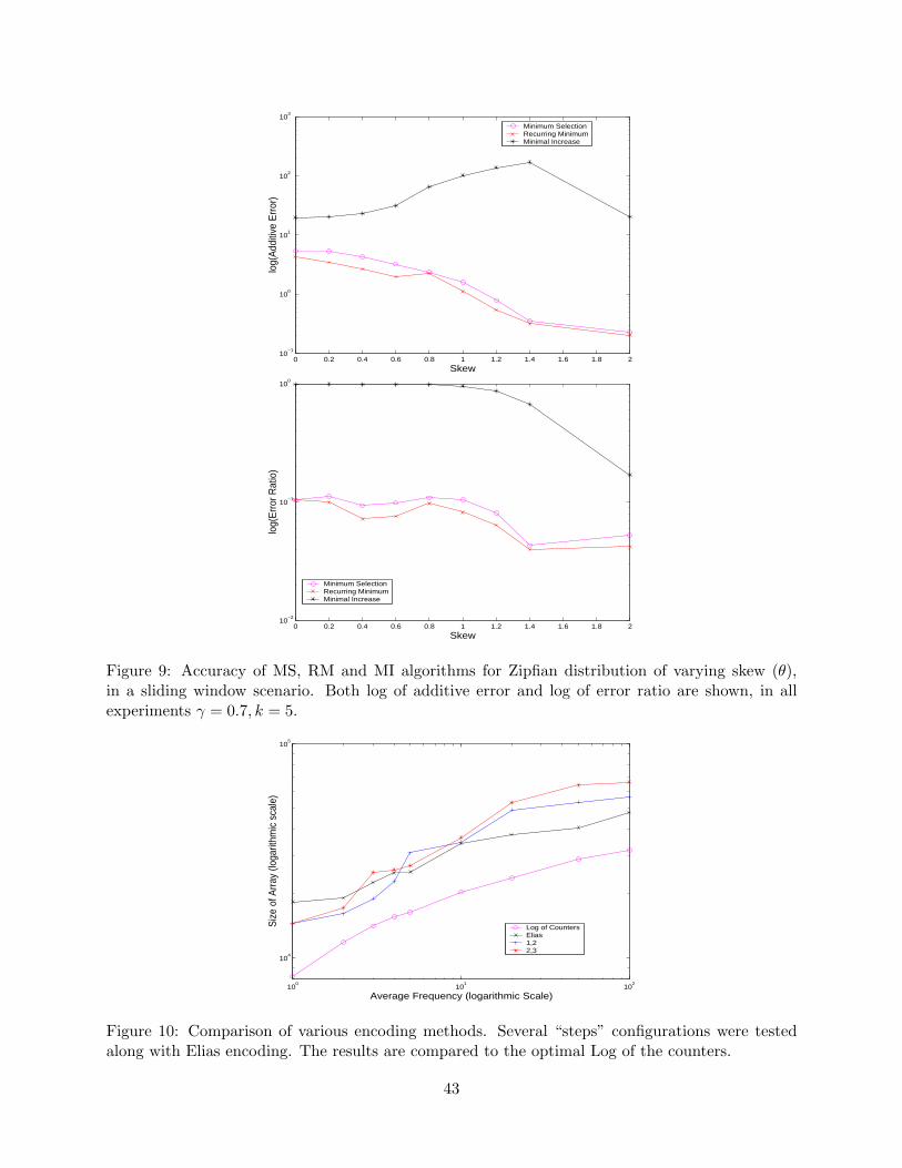
0 0.2 0.4 0.6 0.8 1 1.2 1.4 1.6 1.8 210

−1

100

101

102

103

Skew

log(

Add

itive

Err

or)

Minimum SelectionRecurring MinimumMinimal Increase

0 0.2 0.4 0.6 0.8 1 1.2 1.4 1.6 1.8 210

−2

10−1

100

Skew

log(

Err

or R

atio

)

Minimum SelectionRecurring MinimumMinimal Increase

Figure 9: Accuracy of MS, RM and MI algorithms for Zipfian distribution of varying skew (θ),in a sliding window scenario. Both log of additive error and log of error ratio are shown, in allexperiments γ = 0.7, k = 5.

100

101

102

104

105

Average Frequency (logarithmic Scale)

Siz

e of

Arr

ay (l

ogar

ithm

ic s

cale

)

Log of CountersElias 1,2 2,3

Figure 10: Comparison of various encoding methods. Several “steps” configurations were testedalong with Elias encoding. The results are compared to the optimal Log of the counters.

43

0 1 2 3 4 5 6 7 8 9 10

x 105

0

1000

2000

3000

4000

5000

6000

7000

8000

9000

Size of array

Tim

e (m

s)

Static build timeUpdate time Lookup time

103

104

105

106

0

0.005

0.01

0.015

0.02

0.025

Size of array (logarithmic scale)

Tim

e (m

s)

Static build timeUpdate time Lookup time

Figure 11: String-array index performance over various array sizes. The first graph presents totaltimes, while the second shows time per action.

44

in the SBF to the hash table, to create maximum match between the two schemes. We executedthe same performance check described above for this setup, comparing the performance of the twomethods.

The results of this test are shown in Figure 12. It is important to remember that every lookupin the SBF translates to k lookups, and the same is true for updates, giving the hash table aninherent advantage in this comparison. However, as items are hashed into the table and collisionsaccumulate, the complexity of the actions performed by the hash table increase. The SBF suffersno such penalties and perform the same number of lookups and updates with no regards to the hit-ratio within its counters vector. Note that the results for lookups are measured after the insertions,where collisions might affect them.

It is evident from the results that the SBF is, as expected, somewhat slower than the hashtable. However, for larger table sizes, the hash table is only about twice as fast as the SBF, wherewe would expect a ratio closer to k. In fact, there is a degradation in the performance of the hashtable as the size increases, which can only be explained by the fact that the hash functions are notperfectly random, and have some effect of clustering of results. When the size of the table increases,this results in several buckets hashing a large number of items, thus affecting the average complexityof a lookup into the table. This effect exists in the SBF as well, but it does not manifest itself inthe performance (since collisions do not cause additional actions), but might result in higher errorratios.

Storage The second important aspect that was tested is the storage required by the string-arrayindex. We used the same setting described above, and checked the size (in bits) required for everypart of the structure. The results shown in Figure 13 compare the size of the string-array index tothe raw size of the bit vector that holds the counters. This comparison is performed for the emptyarray (average frequency = 0) and for the array after the insertions (average frequency = 10). Thesize of the bit array includes the slacks, with slack ratio of 0.5, meaning that 0.5 bits are addedto the size of the bit array per item. The sizes of the bit array before and after the insertions arealmost identical, thanks to the usage of the slacks, which (mostly) prevent the need to reallocatethe array and increase its size.

The comparison shows that for a bit vector size of N , the string-array index requires about1.5N bits in the initial state, and about 2N bits in the final state. This difference is explainedin the graphs shown in Figure 14, which divide the total storage into its various components. Acomparison between the two graphs clearly shows that for the empty array there is almost no needfor 3rd level offset vectors, since all subgroups are small enough to use the lookup table. However,in the filled array, there is a considerable number of groups that are too large to be handled by thelookup table, requiring that offset vectors be built for them. This is the major difference betweenthe results in the two scenarios, and explain the rise in the size of the string-array index. This sizeincrease is unique to the initial stage, though, and does not continue further when more insertionsare introduced into the string-array index, so the storage stabilizes at about 2− 2.5N bits.

Next we compare the storage needed for the string-array index with the storage a regular hashtable would require. Both structures require storing of the counter values themselves, with eachstructure relying on additional storage: the string-array index needs the entire offset storage, whilethe hash table needs to store the keys themselves, in order to resolve collisions in lookups. Thestorage needed by the hash table for m distinct keys can be described as m log m, assuming thatthe keys are integers of the domain [1..m], or for a tighter estimate, the total size is

∑mi=1 log i. We

compare those numbers to the additional storage required by the string-array index. Those resultsare shown at Figure 15, and display a clear advantage to the string-array index.

45

0 1 2 3 4 5 6 7 8 9 10

x 105

0

1

2

3

4

5

6

7

8x 10

4

Size of array (items)

Tim

e (m

s)

SBF Static build timeSBF Update timeSBF Lookup timeHash Static build timeHash Update timeHash Lookup time

103

104

105

106

0

0.01

0.02

0.03

0.04

0.05

0.06

0.07

0.08

0.09

Size of array (items − logarithmic scale)

Tim

e (m

s)

SBF Static build timeSBF Update timeSBF Lookup timeHash Static build timeHash Update timeHash Lookup time

Figure 12: Performance of the SBF compared to the LEDA implementation of hash table, forvarious table sizes. The SBF uses k = 5, m equal to the size of the hash table. First graph displaystotal results, second graph shows results per-action.

46

1 5 10 25 50 100 250 5000

2

4

6

8

10

12

14

16x 10

5

Size of array (X1000 items)

Arra

y stor

age s

ize (b

its)

SAI − Avg. freq. = 0 Bit vector − Avg. freq. = 0 SAI − Avg. freq. = 10 Bit vector − Avg. freq. = 10

Figure 13: Size comparison between the bit vector (raw storage) and string-array index (indexstructure), for various array sizes. Results show two scenarios - an empty array (average frequency= 0), and average frequency = 10.

1 5 10 25 50 100 250 5000

0.2

0.4

0.6

0.8

1

1.2

1.4

1.6

1.8

2x 10

6

Size of array (X1000 items)

Arra

y sto

rage

size

(bits

)

Bit Array size L1 Coarse offset vectorL2 offset vectors L3 offset vectors Lookup table

1 5 10 25 50 100 250 5000

0.5

1

1.5

2

2.5x 10

6

Size of array (X1000 items)

Arra

y sto

rage

size

(bits

)

Bit Array size L1 Coarse offset vectorL2 offset vectors L3 offset vectors Lookup table

Figure 14: Breakup of the total size required to the different parts of the string-array index struc-ture. First graph shows average frequency of 0, the second shows average frequency of 10.

47

1 5 10 25 50 100 250 5000

1

2

3

4

5

6

7

8

9

10x 10

6

Size of array (*1000 items)

Arra

y st

orag

e si

ze (b

its)

SAI − Avg. freq. = 0SAI − Avg. freq. = 10Hash table − nlognSum of logs

Figure 15: Storage size comparison between the string-array index and a conventional hash table.Sizes compared are the additional storage besides the counters. Hash table sizes are given asm log2 m (loose estimate) and

∑mi=1 log2 i (tighter estimate).

Another option for hash tables usage involves using perfect hashing. This scheme prevents theneed for storage of the keys themselves, because no collisions are possible. However, perfect hashinghas several disadvantages in our case: those functions do not perform well in the dynamic case.Usually, to create a perfect hashing function, the set of keys has to be known in advance. Anotherlimitation is the size and complexity of the function itself (and its generation). A perfect hashingfunction requires a considerable space - O(m log m), making it as expensive as a standard hashtable, storage-wise.

7 Conclusions

This report presented Spectral Bloom Filters, extending Bloom Filters by storing counters insteadof bit flags. The structure supports updates and deletions, while preserving storage size of N +o(N) + O(m) bits. We presented several heuristics for insertions and lookups in a SBF. MinimumSelection uses the same logic as the original Bloom Filter. Minimal Increase is a simple yet powerfulheuristic with very low error rates, but no support for updates and deletions. Recurring Minimumuses a secondary storage to take care of “problematic” cases, and it supports deletions and updateswith no accuracy loss. We also present the string-array index, a data structure which providefast access to variable-length encoded data while being compact enough to be used in the SpectralBloom Filter. We show its structure and maintenance for static data and during dynamic changesin the data-set.

Several experiments show the error rates the Spectral Bloom Filter provides for several config-urations. The SBF was tested using synthetic data with Zipfian distribution, and using real-lifedata. The error rates of using the Recurring Minimum or Minimal Increase heuristics proved tobe significantly better than those of the Minimum Selection algorithm. We also compared thesemethods when facing deletions and updates, in which case the Minimal Increase method revealsits main weakness and becomes the least successful of the three. We have experimented withthe string-array index structure, testing its storage requirements and performance. The structureproved to be efficient in its storage needs, while performing fast lookup queries and updates.

There are several extensions to the basic functionality of the SBF. One property is the ability to

48

union sets effectively, provided that the same parameters are used (hash functions and array size).For such Bloom Filters, a union of two data sets only requires an addition of the counter vectorsrepresenting them. The SBF can support both streaming data and sliding window data sets, giventhat old data is available for deletion.

The SBF enables new applications, and enables more effective execution of existing applications.SBFs can be used for maintaining demographics of a multiset or set, and allow data profiling andfiltering using an arbitrary threshold. It can be used for ad-hoc iceberg-queries, where the thresholddefining the query is not known in construction time, or changes as the data is queried. BifocalSampling can use SBF as an index data structure in the sparse-any procedure (in fact, SBF can beused in any join of type t-index ). The SBF can also be plugged into many applications currentlyusing Bloom Filters. For example, Bloomjoins can be extended using SBF, with better efficiencyfor many types of queries.

References

[AMS99] N. Alon, Y. Matias, and M. Szegedy. The space complexity of approximating thefrequency moments. Journal of Computer and System Sciences, 58(1):148–173, 1999.

[Arc] The UCI KDD Archive. http://kdd.ics.uci.edu.

[BBD+02] Brian Babcock, Shivnath Babu, Mayur Datar, Rajeev Motwani, and Jennifer Widom.Models and issues in data stream systems. In Proceedings of the twenty-first ACMSIGMOD-SIGACT-SIGART symposium on Principles of database systems, pages 1–16. ACM Press, 2002.

[Blo70] Burton H. Bloom. Space/time trade-offs in hash coding with allowable errors. Com-munications of the ACM, 13(7):422–426, 1970.

[BM02] Andrei Broder and Michael Mitzenmacher. Network applications of Bloom Filters: Asurvey. In Proceedings of Allerton, 2002.

[Bro02] Andrei Z. Broder. Personal communication. 2002.

[Eli75] Peter Elias. Universal codeword sets and representations of the integers. IEEE Trans-actions on Information Theory, 21(2):194–202, 1975.

[EV02] Cristian Estan and George Varghese. New directions in traffic measurement and ac-counting. In Proceedings of ACM SIGCOMM, pages 323–336. ACM Press, 2002.

[FCA] Li Fan, Pei Cao, and Jussara Almeida. A prototype implementation of summary-cacheenhanced icp in squid 1.1.14. www.cs.wisc.edu/˜ cao/sc-icp.html.

[FCAB98] Li Fan, Pei Cao, Jussara Almeida, and Andrei Z. Broder. Summary cache: a scalablewide-area web cache sharing protocol. ACM SIGCOMM Computer CommunicationReview, 28(4):254–265, 1998.

[FSGM+98] Min Fang, Narayanan Shivakumar, Hector Garcia-Molina, Rajeev Motwani, and Jef-frey D. Ullman. Computing iceberg queries efficiently. In Proc. of 24th InternationalConference on Very Large Data Bases, VLDB, pages 299–310, 24–27 1998.

49

[GGMS96] Sumit Ganguly, Phillip B. Gibbons, Yossi Matias, and Avi Silberschatz. Bifocal sam-pling for skew-resistant join size estimation. In Proceedings of the 15th ACM SIGMODinternational conference on Management of data, pages 271–281. ACM Press, 1996.

[GM98] Phillip B. Gibbons and Yossi Matias. New sampling-based summary statistics forimproving approximate query answers. In Proceedings ACM SIGMOD InternationalConference on Management of Data, Seattle, Washington, USA, pages 331–342. ACMPress, 1998.

[GM99] Phillip B. Gibbons and Yossi Matias. Synopsis data structures for massive data sets.DIMACS: Series in Discrete Mathematics and Theoretical Computer Science: SpecialIssue on External Memory Algorithms and Visualization, A, 1999.

[Gre82] Lee L. Gremillion. Designing a bloom filter for differential file access. Communicationsof the ACM, 25(9):600–604, 1982.

[HNSS93] P. J. Haas, J. F. Naughton, S. Seshadri, and A. N. Swami. Fixed-precision estimationof join selectivity. In Proceedings of the 12th ACM Symp. on Principles of DatabaseSystems, pages 190–201, 1993.

[Jac89] Guy Jacobson. Space-efficient static trees and graphs. In Proceedings of the 30th IEEESymposium on Foundations of Computer Science, pages 549–554, 1989.

[LED] LEDA - Library of Efficient Data Types and Algorithms. http://www.algorithmic-solutions.com/enleda.htm.

[Mat] Yossi Matias. Bloom histograms. Unpublished manuscript, July 2001.

[Mit01] Michael Mitzenmacher. Compressed bloom filters. In Proceedings of the twentiethannual ACM symposium on Principles of distributed computing, pages 144–150. ACMPress, 2001.

[ML86] Lothar F. Mackert and Guy M. Lohman. R* optimizer validation and performanceevaluation for distributed queries. In Proc. of 12th International Conference on VeryLarge Data Bases, VLDB, pages 149–159. Morgan Kaufmann, 1986.

[MM02] G. S. Manku and R. Motwani. Approximate frequency counts over data streams. InProc. of the 28th International Conference on Very Large Data Bases, VLDB, pages346–357, 2002.

[Mun96] J. Ian Munro. Tables. In Proceedings of the 16th Foundations of Software Technologyand Theoretical Computer Science (FST & TCS), volume 1180 of Lecture notes inComputer sci., pages 37–42. Springer-Verlag, Berlin, 1996.

[MW94] Udi Manber and Sun Wu. An algorithm for approximate membership checking withapplication to password security. Information Processing Letters, 50(4):191–197, 1994.

[RK02] S. Rhea and J. Kubiatowicz. Probabilistic location and routing. In Proceedings of the21st Annual Joint Conference of the IEEE Computer and Communications Societies(INFOCOM), 2002.

[RRR00] Rajeev Raman, Venkatesh Raman, and S. Srinivasa Rao. Succinct dynamic datastructures. Lecture Notes in Computer Science, 2125:426–437, 2000.

50

[Squ] Squid Web Proxy Cache. http://www.squid-cache.org.

[Zip49] G.K. Zipf. Human behaviour and the principle of least effort. Addison–Wesley press,1949.

51