Spectral and Decomposition Trackingfor Rendering Heterogeneous Volumes

authored by Peter Kutz, Ralf Habel, Karl Li, and Jan Novákand presented by Peter Kutz

Hi, I’m Peter Kutz and this talk is about the paper Spectral and Decomposition Tracking for Rendering Heterogeneous Volumes.

In this work, our focus is more efficient unbiased rendering of volumes, in particular volumes that are chromatic and heterogeneous. Chromatic means that their scattering and absorption properties vary for different wavelengths of light, and heterogeneous means that their properties vary throughout space.

In this work, our focus is more efficient unbiased rendering of volumes, in particular volumes that are chromatic and heterogeneous. Chromatic means that their scattering and absorption properties vary for different wavelengths of light, and heterogeneous means that their properties vary throughout space.

Chromatic

In this work, our focus is more efficient unbiased rendering of volumes, in particular volumes that are chromatic and heterogeneous. Chromatic means that their scattering and absorption properties vary for different wavelengths of light, and heterogeneous means that their properties vary throughout space.

Chromatic

Heterogeneous

In this work, our focus is more efficient unbiased rendering of volumes, in particular volumes that are chromatic and heterogeneous. Chromatic means that their scattering and absorption properties vary for different wavelengths of light, and heterogeneous means that their properties vary throughout space.

Decomposition Tracking for Increased Speed

Spectral Tracking for Reduced VarianceIntegral Formulation of Null-Collision Algorithms

Delta Tracking

Putting It All Together

First we will review delta tracking, which is the foundation of our work.Then we will introduce our decomposition tracking.We will also show the integral formulation of null-collision algorithms.Then we will introduce our spectral tracking.Finally we will describe how our new algorithms can be put together.

Decomposition Tracking for Increased Speed

Spectral Tracking for Reduced VarianceIntegral Formulation of Null-Collision Algorithms

Delta Tracking

Putting It All Together

First we will review delta tracking, which is the foundation of our work.Then we will introduce our decomposition tracking.We will also show the integral formulation of null-collision algorithms.Then we will introduce our spectral tracking.Finally we will describe how our new algorithms can be put together.

Decomposition Tracking for Increased Speed

Spectral Tracking for Reduced VarianceIntegral Formulation of Null-Collision Algorithms

Delta Tracking

Putting It All Together

First we will review delta tracking, which is the foundation of our work.Then we will introduce our decomposition tracking.We will also show the integral formulation of null-collision algorithms.Then we will introduce our spectral tracking.Finally we will describe how our new algorithms can be put together.

Decomposition Tracking for Increased Speed

Spectral Tracking for Reduced VarianceIntegral Formulation of Null-Collision Algorithms

Delta Tracking

Putting It All Together

First we will review delta tracking, which is the foundation of our work.Then we will introduce our decomposition tracking.We will also show the integral formulation of null-collision algorithms.Then we will introduce our spectral tracking.Finally we will describe how our new algorithms can be put together.

Decomposition Tracking for Increased Speed

Spectral Tracking for Reduced VarianceIntegral Formulation of Null-Collision Algorithms

Delta Tracking

Putting It All Together

First we will review delta tracking, which is the foundation of our work.Then we will introduce our decomposition tracking.We will also show the integral formulation of null-collision algorithms.Then we will introduce our spectral tracking.Finally we will describe how our new algorithms can be put together.

Decomposition Tracking for Increased Speed

Spectral Tracking for Reduced VarianceIntegral Formulation of Null-Collision Algorithms

Delta Tracking

Putting It All Together

First we will review delta tracking, which is the foundation of our work.Then we will introduce our decomposition tracking.We will also show the integral formulation of null-collision algorithms.Then we will introduce our spectral tracking.Finally we will describe how our new algorithms can be put together.

Decomposition Tracking for Increased Speed

Spectral Tracking for Reduced VarianceIntegral Formulation of Null-Collision Algorithms

Delta Tracking

Putting It All Together

First we will review delta tracking, which is the foundation of our work.Then we will introduce our decomposition tracking.We will also show the integral formulation of null-collision algorithms.Then we will introduce our spectral tracking.Finally we will describe how our new algorithms can be put together.

Delta Tracking

Let’s get started with delta tracking.

(homogeneous volume)

Here’s a schematic 2D diagram of a rectangular volume, which can be thought of as being composed of particles. This happens to be a homogeneous volume, one with the same properties throughout. It has a uniform density.

The ultimate goal of volume rendering and of our work is to generate paths of light between a light source and the camera.

The ultimate goal of volume rendering and of our work is to generate paths of light between a light source and the camera.

However our focus is the efficient generation of individual path segments, or free paths. For a homogeneous volume like this one this is relatively easy.

The distribution of scattering and absorption distances is exponential, proportional to the transmittance, and we can draw samples from an exponential distribution directly.

1

1/2

1/4

1/81/161/32

1 2 3 4 50

The distribution of scattering and absorption distances is exponential, proportional to the transmittance, and we can draw samples from an exponential distribution directly.

Closed-Form Tracking

[Ulam & von Neumann 1947]

This sampling process is called closed-form tracking, and it immediately gives us a scattering or absorption location. For simplicity, we’ll mainly just talk about scattering in this presentation, but sampling absorption works analogously.

Closed-Form Tracking

[Ulam & von Neumann 1947]

This sampling process is called closed-form tracking, and it immediately gives us a scattering or absorption location. For simplicity, we’ll mainly just talk about scattering in this presentation, but sampling absorption works analogously.

distance

extinction

Closed-Form Tracking

[Ulam & von Neumann 1947]

Here’s a different view of the process for the slice of the volume along the ray, with the distance along the ray on the horizontal axis and the density, or, more precisely, the extinction coefficient, on the vertical axis. We simply sample a single distance from the exponential distribution and that tells us the scattering location.

distance

extinction

Closed-Form Tracking

[Ulam & von Neumann 1947]

Here’s a different view of the process for the slice of the volume along the ray, with the distance along the ray on the horizontal axis and the density, or, more precisely, the extinction coefficient, on the vertical axis. We simply sample a single distance from the exponential distribution and that tells us the scattering location.

distance

extinction

Closed-Form Tracking

[Ulam & von Neumann 1947]

Here’s a different view of the process for the slice of the volume along the ray, with the distance along the ray on the horizontal axis and the density, or, more precisely, the extinction coefficient, on the vertical axis. We simply sample a single distance from the exponential distribution and that tells us the scattering location.

distance

extinction

Closed-Form Tracking

[Ulam & von Neumann 1947]

Here’s a different view of the process for the slice of the volume along the ray, with the distance along the ray on the horizontal axis and the density, or, more precisely, the extinction coefficient, on the vertical axis. We simply sample a single distance from the exponential distribution and that tells us the scattering location.

(heterogeneous volume)

But what if we want to find a scattering location in a heterogeneous volume like this one? This volume has a somewhat arbitrary shape and nonuniform density.

So instead of the distribution of scattering locations being exponential…

So instead of the distribution of scattering locations being exponential…

…it can be some arbitrary shape.

…it can be some arbitrary shape.

But let’s observe that this cloud is actually a subset of the homogeneous box that we looked at before:

The idea of delta tracking is to use the closed-form homogeneous-volume sampling to sample a heterogeneous volume. This is done by converting some of these real particles to fictitious particles to create a homogeneous version of our heterogeneous volume:

= real= fictitious

[Butcher & Messel 1958; Zerby et al. 1961]

Delta tracking works by repeatedly sampling a distance from the combined volume, and then checking whether a real or fictitious particle was hit. Whenever a fictitious particle is hit, we just continue in the same direction. When a real particle is hit, we scatter. This algorithm perfectly importance samples the transmittance, producing the desired distribution of scatter distances.

By the way, delta tracking is also known as Woodcock tracking, after a 1965 paper, but we found a 1961 paper by Zerby that introduced virtually the same technique and in much more detail. The algorithm in the Zerby paper is partially based on some similar techniques introduced in 1958 and 1960 papers by Butcher and Messel.

= real= fictitiousDelta Tracking

[Butcher & Messel 1958; Zerby et al. 1961]

Delta tracking works by repeatedly sampling a distance from the combined volume, and then checking whether a real or fictitious particle was hit. Whenever a fictitious particle is hit, we just continue in the same direction. When a real particle is hit, we scatter. This algorithm perfectly importance samples the transmittance, producing the desired distribution of scatter distances.

By the way, delta tracking is also known as Woodcock tracking, after a 1965 paper, but we found a 1961 paper by Zerby that introduced virtually the same technique and in much more detail. The algorithm in the Zerby paper is partially based on some similar techniques introduced in 1958 and 1960 papers by Butcher and Messel.

= real= fictitiousDelta Tracking

[Butcher & Messel 1958; Zerby et al. 1961]

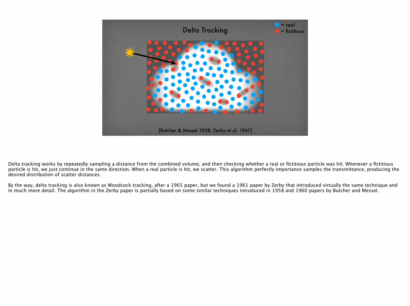
Delta tracking works by repeatedly sampling a distance from the combined volume, and then checking whether a real or fictitious particle was hit. Whenever a fictitious particle is hit, we just continue in the same direction. When a real particle is hit, we scatter. This algorithm perfectly importance samples the transmittance, producing the desired distribution of scatter distances.

By the way, delta tracking is also known as Woodcock tracking, after a 1965 paper, but we found a 1961 paper by Zerby that introduced virtually the same technique and in much more detail. The algorithm in the Zerby paper is partially based on some similar techniques introduced in 1958 and 1960 papers by Butcher and Messel.

= real= fictitiousDelta Tracking

[Butcher & Messel 1958; Zerby et al. 1961]

Delta tracking works by repeatedly sampling a distance from the combined volume, and then checking whether a real or fictitious particle was hit. Whenever a fictitious particle is hit, we just continue in the same direction. When a real particle is hit, we scatter. This algorithm perfectly importance samples the transmittance, producing the desired distribution of scatter distances.

By the way, delta tracking is also known as Woodcock tracking, after a 1965 paper, but we found a 1961 paper by Zerby that introduced virtually the same technique and in much more detail. The algorithm in the Zerby paper is partially based on some similar techniques introduced in 1958 and 1960 papers by Butcher and Messel.

distance

= real= fictitiousDelta Tracking

extinction

[Butcher & Messel 1958; Zerby et al. 1961]

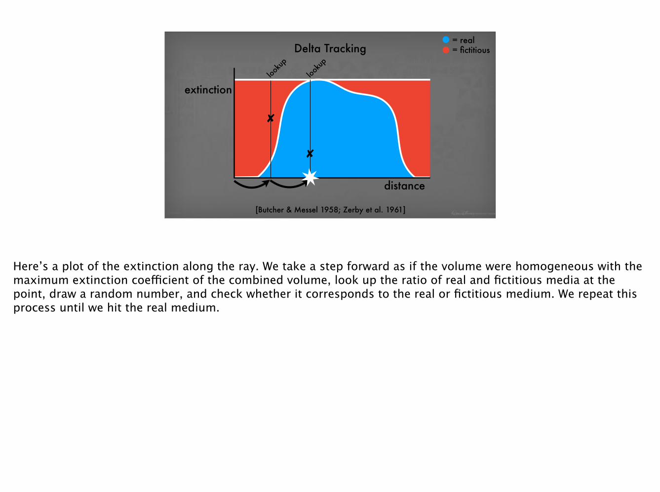
Here’s a plot of the extinction along the ray. We take a step forward as if the volume were homogeneous with the maximum extinction coefficient of the combined volume, look up the ratio of real and fictitious media at the point, draw a random number, and check whether it corresponds to the real or fictitious medium. We repeat this process until we hit the real medium.

distance

= real= fictitiousDelta Tracking

extinction

[Butcher & Messel 1958; Zerby et al. 1961]

Here’s a plot of the extinction along the ray. We take a step forward as if the volume were homogeneous with the maximum extinction coefficient of the combined volume, look up the ratio of real and fictitious media at the point, draw a random number, and check whether it corresponds to the real or fictitious medium. We repeat this process until we hit the real medium.

distance

= real= fictitiousDelta Tracking

extinctionloo

kup

[Butcher & Messel 1958; Zerby et al. 1961]

Here’s a plot of the extinction along the ray. We take a step forward as if the volume were homogeneous with the maximum extinction coefficient of the combined volume, look up the ratio of real and fictitious media at the point, draw a random number, and check whether it corresponds to the real or fictitious medium. We repeat this process until we hit the real medium.

distance

= real= fictitiousDelta Tracking

extinctionloo

kup

[Butcher & Messel 1958; Zerby et al. 1961]

Here’s a plot of the extinction along the ray. We take a step forward as if the volume were homogeneous with the maximum extinction coefficient of the combined volume, look up the ratio of real and fictitious media at the point, draw a random number, and check whether it corresponds to the real or fictitious medium. We repeat this process until we hit the real medium.

distance

= real= fictitiousDelta Tracking

extinctionloo

kup

[Butcher & Messel 1958; Zerby et al. 1961]

Here’s a plot of the extinction along the ray. We take a step forward as if the volume were homogeneous with the maximum extinction coefficient of the combined volume, look up the ratio of real and fictitious media at the point, draw a random number, and check whether it corresponds to the real or fictitious medium. We repeat this process until we hit the real medium.

distance

= real= fictitiousDelta Tracking

extinctionloo

kup

looku

p

[Butcher & Messel 1958; Zerby et al. 1961]

Here’s a plot of the extinction along the ray. We take a step forward as if the volume were homogeneous with the maximum extinction coefficient of the combined volume, look up the ratio of real and fictitious media at the point, draw a random number, and check whether it corresponds to the real or fictitious medium. We repeat this process until we hit the real medium.

distance

= real= fictitiousDelta Tracking

extinctionloo

kup

looku

p

[Butcher & Messel 1958; Zerby et al. 1961]

Here’s a plot of the extinction along the ray. We take a step forward as if the volume were homogeneous with the maximum extinction coefficient of the combined volume, look up the ratio of real and fictitious media at the point, draw a random number, and check whether it corresponds to the real or fictitious medium. We repeat this process until we hit the real medium.

distance

= real= fictitiousDelta Tracking

extinctionloo

kup

looku

p

[Butcher & Messel 1958; Zerby et al. 1961]

Here’s a plot of the extinction along the ray. We take a step forward as if the volume were homogeneous with the maximum extinction coefficient of the combined volume, look up the ratio of real and fictitious media at the point, draw a random number, and check whether it corresponds to the real or fictitious medium. We repeat this process until we hit the real medium.

Decomposition Tracking

Now we have the background necessary to understand decomposition tracking.

memory accesses

procedural evaluations

As we just saw, delta tracking requires a volume property lookup at each step of the algorithm. This usually consists of a memory lookup into a large volumetric data structure, or a procedural evaluation. Especially for highly-scattering volumes, these volume property lookups can become a significant bottleneck. If we could reduce the cost of these lookups, we could reduce render times.

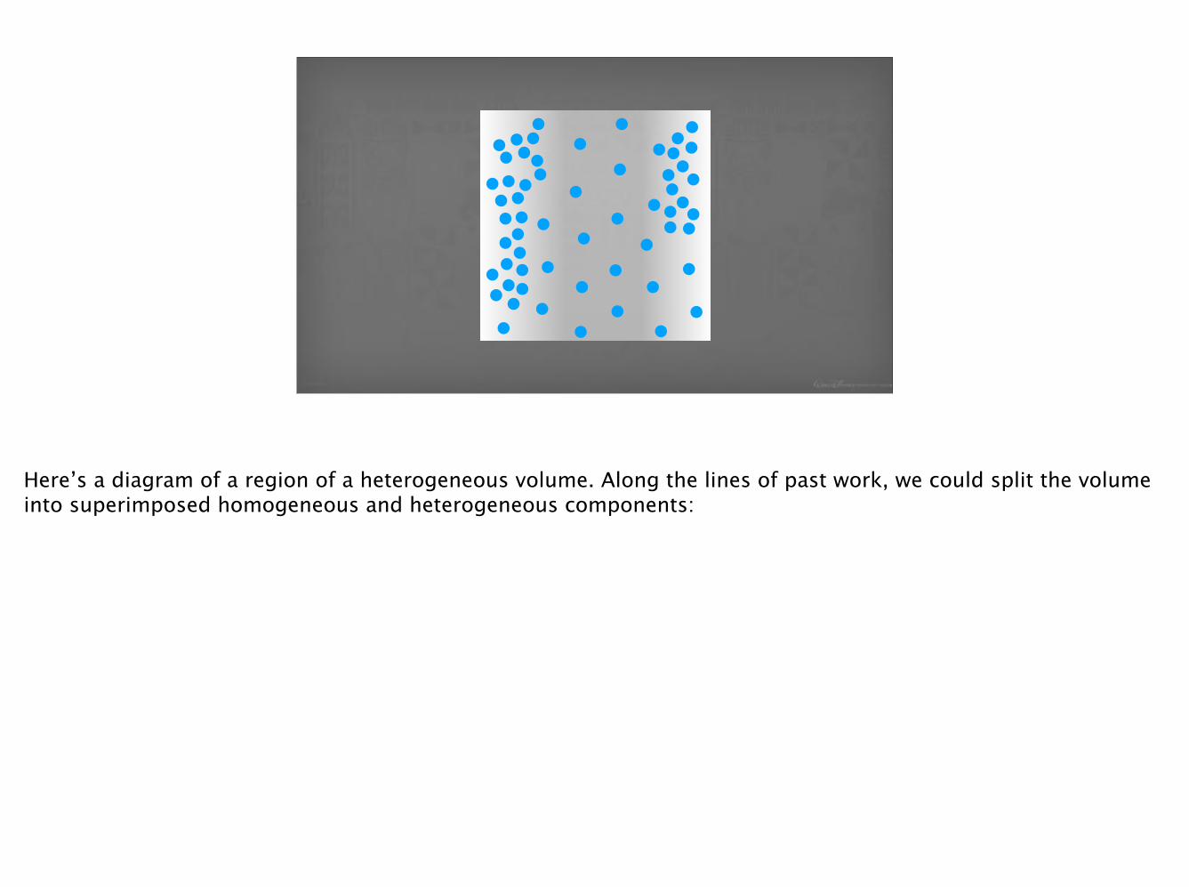
Here’s a diagram of a region of a heterogeneous volume. Along the lines of past work, we could split the volume into superimposed homogeneous and heterogeneous components:

= homogeneous control= heterogeneous residual

[Novák 2014]

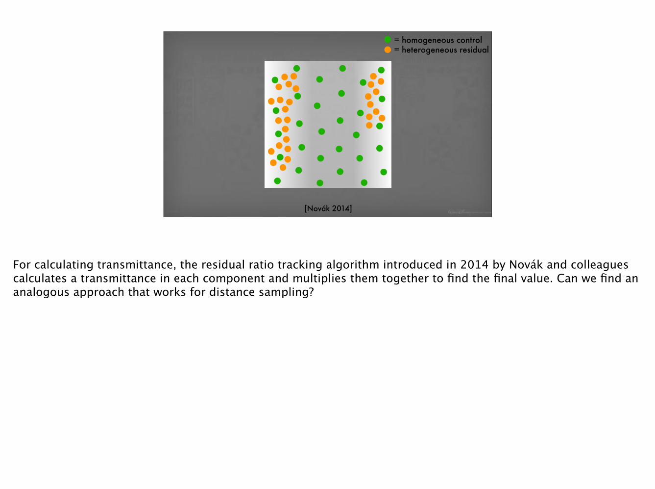
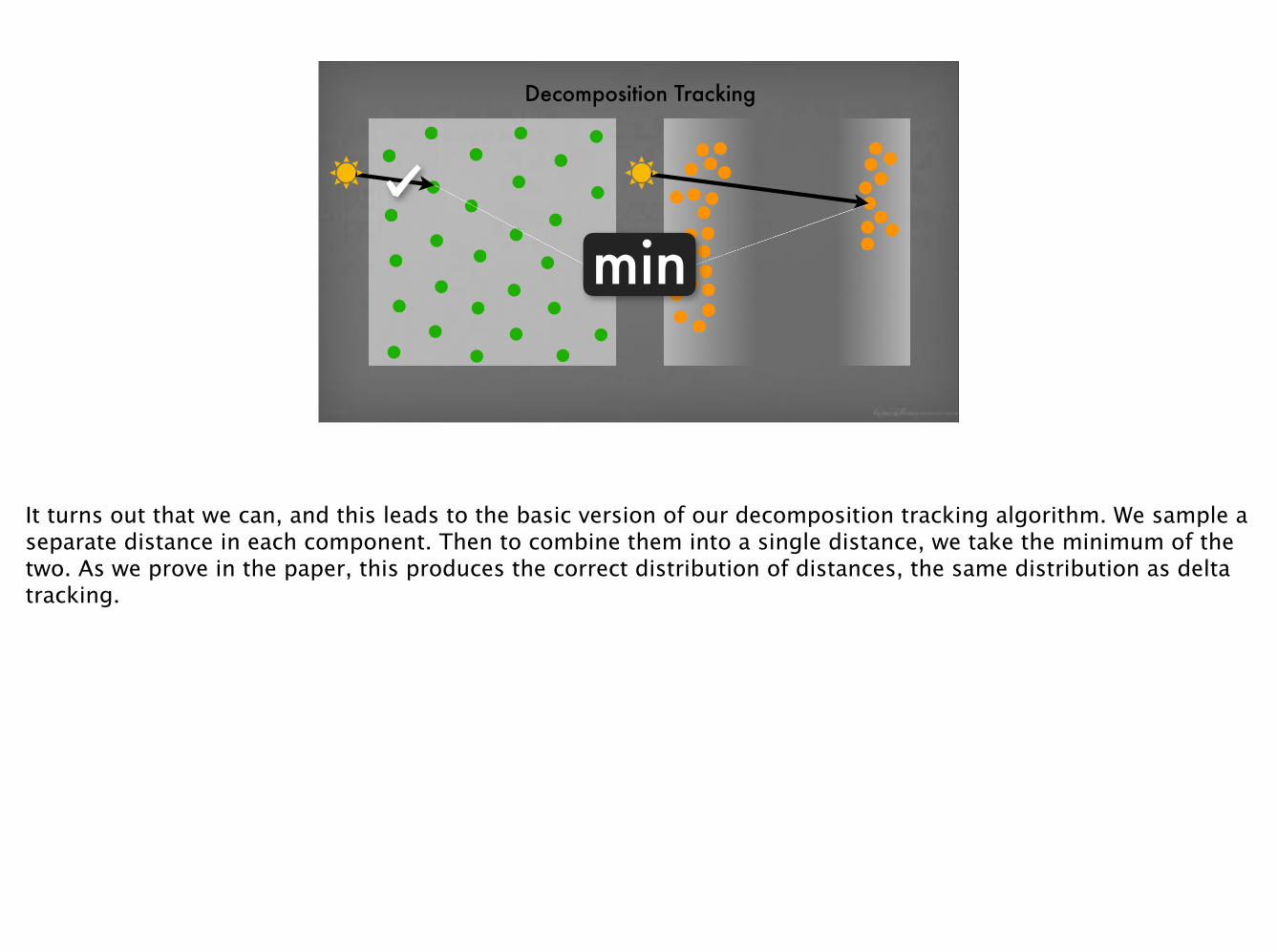
For calculating transmittance, the residual ratio tracking algorithm introduced in 2014 by Novák and colleagues calculates a transmittance in each component and multiplies them together to find the final value. Can we find an analogous approach that works for distance sampling?

It turns out that we can, and this leads to the basic version of our decomposition tracking algorithm. We sample a separate distance in each component. Then to combine them into a single distance, we take the minimum of the two. As we prove in the paper, this produces the correct distribution of distances, the same distribution as delta tracking.

Decomposition Tracking

It turns out that we can, and this leads to the basic version of our decomposition tracking algorithm. We sample a separate distance in each component. Then to combine them into a single distance, we take the minimum of the two. As we prove in the paper, this produces the correct distribution of distances, the same distribution as delta tracking.

Decomposition Tracking

It turns out that we can, and this leads to the basic version of our decomposition tracking algorithm. We sample a separate distance in each component. Then to combine them into a single distance, we take the minimum of the two. As we prove in the paper, this produces the correct distribution of distances, the same distribution as delta tracking.

Decomposition Tracking

min

It turns out that we can, and this leads to the basic version of our decomposition tracking algorithm. We sample a separate distance in each component. Then to combine them into a single distance, we take the minimum of the two. As we prove in the paper, this produces the correct distribution of distances, the same distribution as delta tracking.

distance

Decomposition Tracking

extinction

Here’s a 1D slice of that volume along the ray.

distance

Decomposition Tracking

extinction

= control= residual

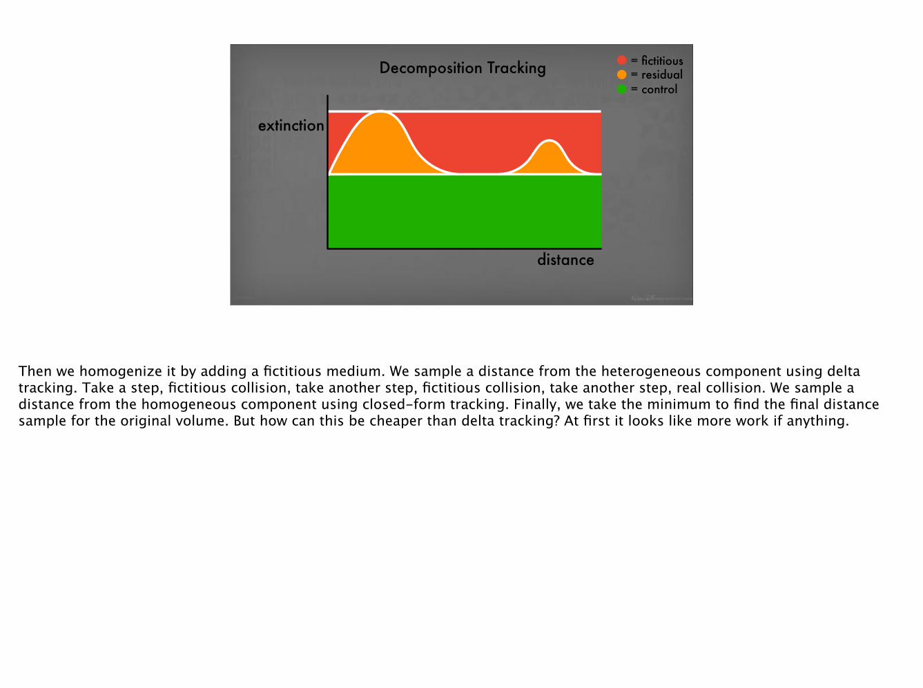
We split it into a homogeneous control and a heterogeneous residual.

distance

Decomposition Tracking

extinction

= control= residual= fictitious

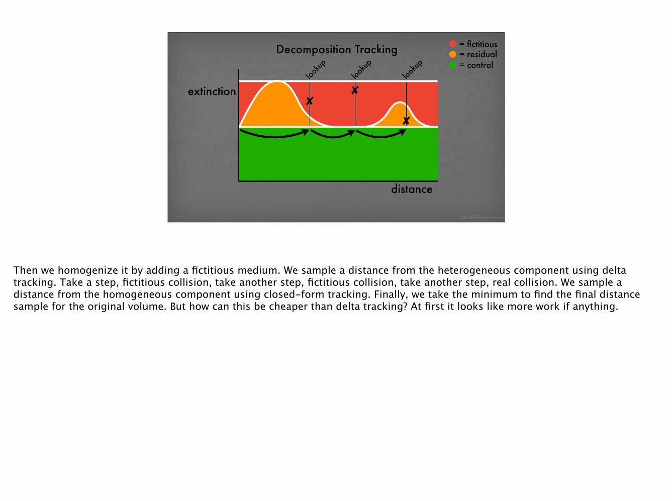
Then we homogenize it by adding a fictitious medium. We sample a distance from the heterogeneous component using delta tracking. Take a step, fictitious collision, take another step, fictitious collision, take another step, real collision. We sample a distance from the homogeneous component using closed-form tracking. Finally, we take the minimum to find the final distance sample for the original volume. But how can this be cheaper than delta tracking? At first it looks like more work if anything.

distance

Decomposition Tracking

extinction

= control= residual= fictitious

Then we homogenize it by adding a fictitious medium. We sample a distance from the heterogeneous component using delta tracking. Take a step, fictitious collision, take another step, fictitious collision, take another step, real collision. We sample a distance from the homogeneous component using closed-form tracking. Finally, we take the minimum to find the final distance sample for the original volume. But how can this be cheaper than delta tracking? At first it looks like more work if anything.

looku

p

distance

Decomposition Tracking

extinction

= control= residual= fictitious

Then we homogenize it by adding a fictitious medium. We sample a distance from the heterogeneous component using delta tracking. Take a step, fictitious collision, take another step, fictitious collision, take another step, real collision. We sample a distance from the homogeneous component using closed-form tracking. Finally, we take the minimum to find the final distance sample for the original volume. But how can this be cheaper than delta tracking? At first it looks like more work if anything.

looku

p

distance

Decomposition Tracking

extinction

= control= residual= fictitious

Then we homogenize it by adding a fictitious medium. We sample a distance from the heterogeneous component using delta tracking. Take a step, fictitious collision, take another step, fictitious collision, take another step, real collision. We sample a distance from the homogeneous component using closed-form tracking. Finally, we take the minimum to find the final distance sample for the original volume. But how can this be cheaper than delta tracking? At first it looks like more work if anything.

looku

p

looku

p

distance

Decomposition Tracking

extinction

= control= residual= fictitious

Then we homogenize it by adding a fictitious medium. We sample a distance from the heterogeneous component using delta tracking. Take a step, fictitious collision, take another step, fictitious collision, take another step, real collision. We sample a distance from the homogeneous component using closed-form tracking. Finally, we take the minimum to find the final distance sample for the original volume. But how can this be cheaper than delta tracking? At first it looks like more work if anything.

looku

p

looku

p

distance

Decomposition Tracking

extinction

= control= residual= fictitious

Then we homogenize it by adding a fictitious medium. We sample a distance from the heterogeneous component using delta tracking. Take a step, fictitious collision, take another step, fictitious collision, take another step, real collision. We sample a distance from the homogeneous component using closed-form tracking. Finally, we take the minimum to find the final distance sample for the original volume. But how can this be cheaper than delta tracking? At first it looks like more work if anything.

looku

p

looku

p

looku

p

distance

Decomposition Tracking

extinction

= control= residual= fictitious

Then we homogenize it by adding a fictitious medium. We sample a distance from the heterogeneous component using delta tracking. Take a step, fictitious collision, take another step, fictitious collision, take another step, real collision. We sample a distance from the homogeneous component using closed-form tracking. Finally, we take the minimum to find the final distance sample for the original volume. But how can this be cheaper than delta tracking? At first it looks like more work if anything.

looku

p

looku

p

looku

p

distance

Decomposition Tracking

extinction

= control= residual= fictitious

Then we homogenize it by adding a fictitious medium. We sample a distance from the heterogeneous component using delta tracking. Take a step, fictitious collision, take another step, fictitious collision, take another step, real collision. We sample a distance from the homogeneous component using closed-form tracking. Finally, we take the minimum to find the final distance sample for the original volume. But how can this be cheaper than delta tracking? At first it looks like more work if anything.

looku

p

looku

p

looku

p

distance

Decomposition Tracking

extinction

= control= residual= fictitious

Then we homogenize it by adding a fictitious medium. We sample a distance from the heterogeneous component using delta tracking. Take a step, fictitious collision, take another step, fictitious collision, take another step, real collision. We sample a distance from the homogeneous component using closed-form tracking. Finally, we take the minimum to find the final distance sample for the original volume. But how can this be cheaper than delta tracking? At first it looks like more work if anything.

distance

Decomposition Tracking

extinction

= control= residual= fictitious

The key to making this performant is to sample the homogeneous component first. Here’s an illustration. We sample the distance from the homogeneous component using closed-form tracking. Then we begin delta tracking on the heterogeneous component. We take a step, as before. But now, we know the homogeneous distance in advance. And we know that as soon as we step beyond it, it doesn’t matter how far we go because we won’t use it anyway — we know the minimum will be the homogeneous distance. So in this case, we don’t even have to do a single lookup of the spatially varying volume properties.

distance

Decomposition Tracking

extinction

= control= residual= fictitious

The key to making this performant is to sample the homogeneous component first. Here’s an illustration. We sample the distance from the homogeneous component using closed-form tracking. Then we begin delta tracking on the heterogeneous component. We take a step, as before. But now, we know the homogeneous distance in advance. And we know that as soon as we step beyond it, it doesn’t matter how far we go because we won’t use it anyway — we know the minimum will be the homogeneous distance. So in this case, we don’t even have to do a single lookup of the spatially varying volume properties.

distance

Decomposition Tracking

extinction

= control= residual= fictitious

The key to making this performant is to sample the homogeneous component first. Here’s an illustration. We sample the distance from the homogeneous component using closed-form tracking. Then we begin delta tracking on the heterogeneous component. We take a step, as before. But now, we know the homogeneous distance in advance. And we know that as soon as we step beyond it, it doesn’t matter how far we go because we won’t use it anyway — we know the minimum will be the homogeneous distance. So in this case, we don’t even have to do a single lookup of the spatially varying volume properties.

distance

Decomposition Tracking

extinction

= control= residual= fictitious

The key to making this performant is to sample the homogeneous component first. Here’s an illustration. We sample the distance from the homogeneous component using closed-form tracking. Then we begin delta tracking on the heterogeneous component. We take a step, as before. But now, we know the homogeneous distance in advance. And we know that as soon as we step beyond it, it doesn’t matter how far we go because we won’t use it anyway — we know the minimum will be the homogeneous distance. So in this case, we don’t even have to do a single lookup of the spatially varying volume properties.

distance

Decomposition Tracking

extinction

= control= residual= fictitious

looku

p

looku

p

looku

p

The key to making this performant is to sample the homogeneous component first. Here’s an illustration. We sample the distance from the homogeneous component using closed-form tracking. Then we begin delta tracking on the heterogeneous component. We take a step, as before. But now, we know the homogeneous distance in advance. And we know that as soon as we step beyond it, it doesn’t matter how far we go because we won’t use it anyway — we know the minimum will be the homogeneous distance. So in this case, we don’t even have to do a single lookup of the spatially varying volume properties.

delta tracking decomposition tracking

42% fewer lookups

Decomposition tracking let’s us render the exact same image with fewer extinction lookups. It can greatly reduce whatever cost is associated with the spatially varying lookups. The improvements due to the decomposition are proportional to how much of the medium we handle as homogeneous. This poses a challenge: finding a tight lower bound of the extinction for doing the closed-form tracking. This is very similar to finding a tight upper bound for delta tracking, which can be fairly challenging, for instance for procedural volumes. Fortunately, both delta tracking and decomposition tracking can be generalized to work with arbitrary functions, not just those that bound the real extinction.

Integral Formulation of Null-Collision Algorithms

To do this, we take a holistic approach inspired by the integral framework of Galtier and colleagues, which we apply to graphics for the first time. Our algorithms can all be derived from this framework, which is in turn derived directly from the radiative transfer equation.

To do this, we take a holistic approach inspired by the integral framework of Galtier and colleagues, which we apply to graphics for the first time. Our algorithms can all be derived from this framework, which is in turn derived directly from the radiative transfer equation.

L(x,!) =

Z 1

0µ̄(x� t!) exp

✓�Z t

0µ̄(x� s!) ds

◆

⇥ Z 1

0H[⇠e < Pa(x� t!)]

µa(x� t!)

µ̄(x� t!)Pa(x� t!)Le(x� t!,!) d⇠e

Q+

Z 1

0H[⇠s < Ps(x� t!)]

µs(x� t!)

µ̄(x� t!)Ps(x� t!)

h Z

S2

fp(!, !̄)L(x� t!, !̄)d!̄id⇠s

Q+

Z 1

0H[⇠n < Pn(x� t!)]

µn(x� t!)

µ̄(x� t!)Pn(x� t!)L(x� t!,!) d⇠n

�dt

[Galtier et al. 2013; Eymet et al. 2013]

The Integral Formulation of Null-Collision Algorithms

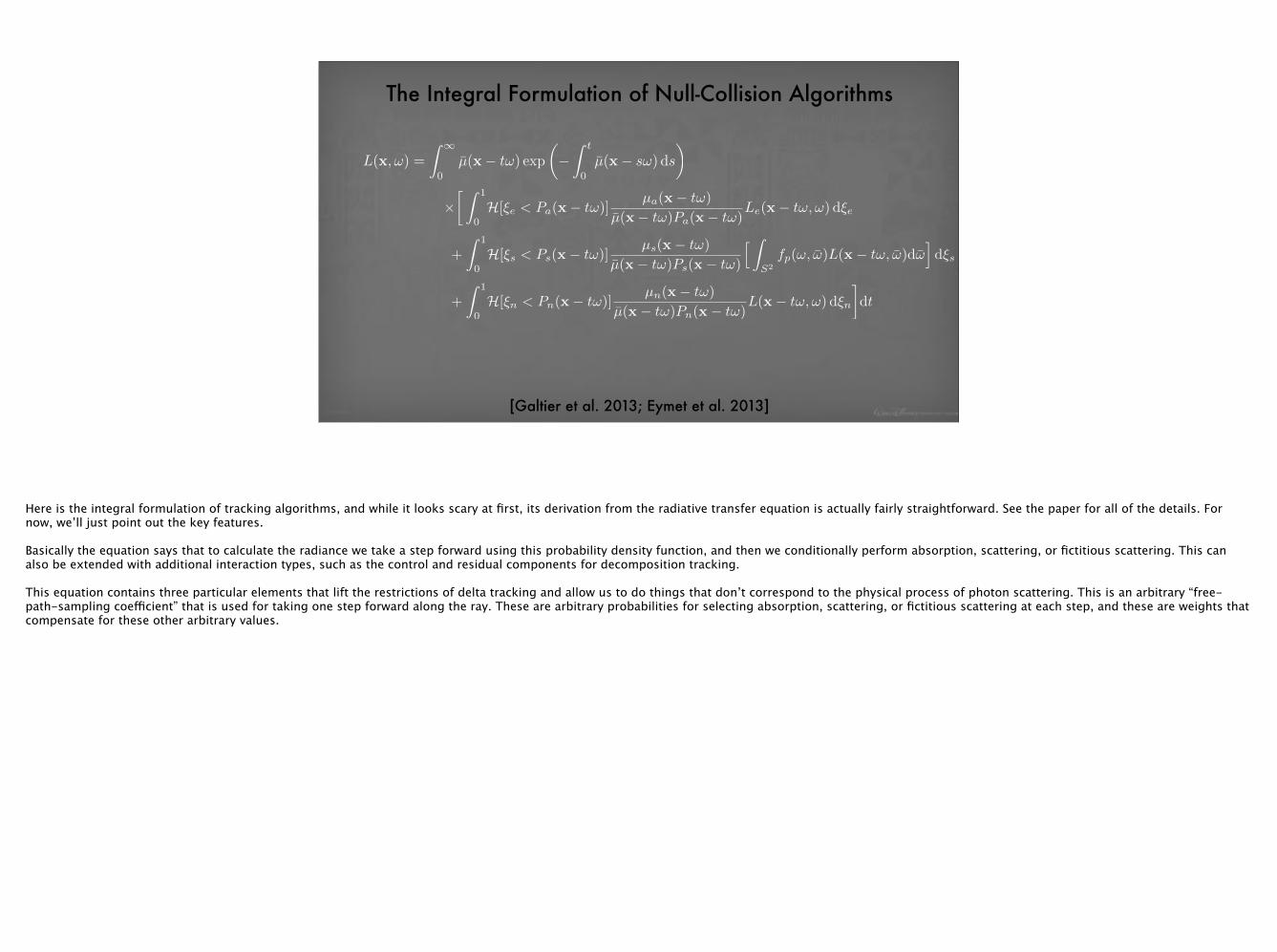
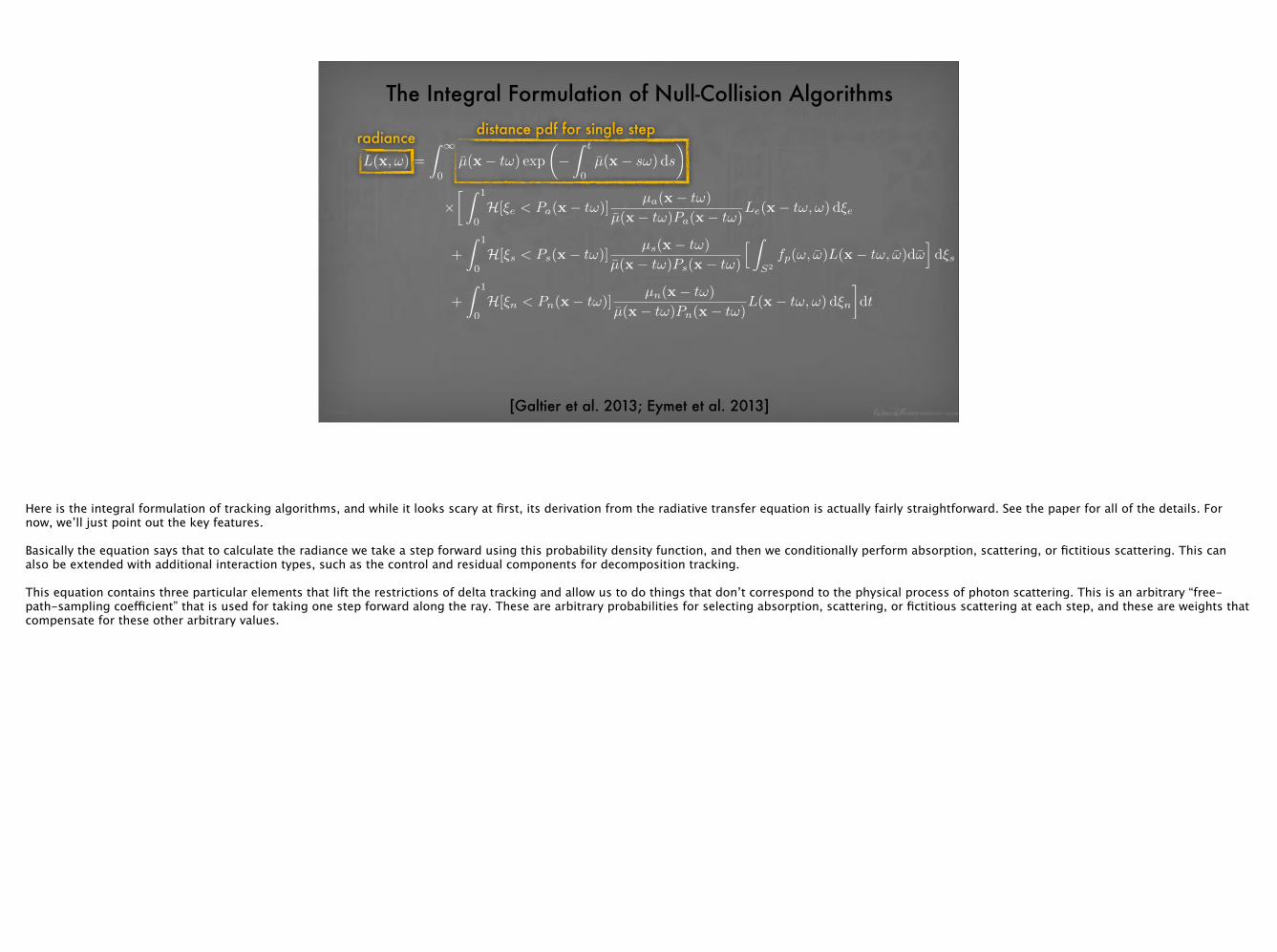
Here is the integral formulation of tracking algorithms, and while it looks scary at first, its derivation from the radiative transfer equation is actually fairly straightforward. See the paper for all of the details. For now, we’ll just point out the key features.

Basically the equation says that to calculate the radiance we take a step forward using this probability density function, and then we conditionally perform absorption, scattering, or fictitious scattering. This can also be extended with additional interaction types, such as the control and residual components for decomposition tracking.

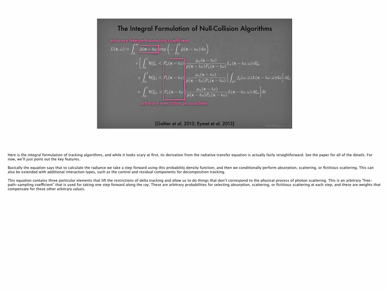
This equation contains three particular elements that lift the restrictions of delta tracking and allow us to do things that don’t correspond to the physical process of photon scattering. This is an arbitrary “free-path-sampling coefficient” that is used for taking one step forward along the ray. These are arbitrary probabilities for selecting absorption, scattering, or fictitious scattering at each step, and these are weights that compensate for these other arbitrary values.

L(x,!) =

Z 1

0µ̄(x� t!) exp

✓�Z t

0µ̄(x� s!) ds

◆

⇥ Z 1

0H[⇠e < Pa(x� t!)]

µa(x� t!)

µ̄(x� t!)Pa(x� t!)Le(x� t!,!) d⇠e

Q+

Z 1

0H[⇠s < Ps(x� t!)]

µs(x� t!)

µ̄(x� t!)Ps(x� t!)

h Z

S2

fp(!, !̄)L(x� t!, !̄)d!̄id⇠s

Q+

Z 1

0H[⇠n < Pn(x� t!)]

µn(x� t!)

µ̄(x� t!)Pn(x� t!)L(x� t!,!) d⇠n

�dt

[Galtier et al. 2013; Eymet et al. 2013]

The Integral Formulation of Null-Collision Algorithms

radiance

Here is the integral formulation of tracking algorithms, and while it looks scary at first, its derivation from the radiative transfer equation is actually fairly straightforward. See the paper for all of the details. For now, we’ll just point out the key features.

Basically the equation says that to calculate the radiance we take a step forward using this probability density function, and then we conditionally perform absorption, scattering, or fictitious scattering. This can also be extended with additional interaction types, such as the control and residual components for decomposition tracking.

This equation contains three particular elements that lift the restrictions of delta tracking and allow us to do things that don’t correspond to the physical process of photon scattering. This is an arbitrary “free-path-sampling coefficient” that is used for taking one step forward along the ray. These are arbitrary probabilities for selecting absorption, scattering, or fictitious scattering at each step, and these are weights that compensate for these other arbitrary values.

L(x,!) =

Z 1

0µ̄(x� t!) exp

✓�Z t

0µ̄(x� s!) ds

◆

⇥ Z 1

0H[⇠e < Pa(x� t!)]

µa(x� t!)

µ̄(x� t!)Pa(x� t!)Le(x� t!,!) d⇠e

Q+

Z 1

0H[⇠s < Ps(x� t!)]

µs(x� t!)

µ̄(x� t!)Ps(x� t!)

h Z

S2

fp(!, !̄)L(x� t!, !̄)d!̄id⇠s

Q+

Z 1

0H[⇠n < Pn(x� t!)]

µn(x� t!)

µ̄(x� t!)Pn(x� t!)L(x� t!,!) d⇠n

�dt

[Galtier et al. 2013; Eymet et al. 2013]

The Integral Formulation of Null-Collision Algorithms

radiance distance pdf for single step

Here is the integral formulation of tracking algorithms, and while it looks scary at first, its derivation from the radiative transfer equation is actually fairly straightforward. See the paper for all of the details. For now, we’ll just point out the key features.

Basically the equation says that to calculate the radiance we take a step forward using this probability density function, and then we conditionally perform absorption, scattering, or fictitious scattering. This can also be extended with additional interaction types, such as the control and residual components for decomposition tracking.

This equation contains three particular elements that lift the restrictions of delta tracking and allow us to do things that don’t correspond to the physical process of photon scattering. This is an arbitrary “free-path-sampling coefficient” that is used for taking one step forward along the ray. These are arbitrary probabilities for selecting absorption, scattering, or fictitious scattering at each step, and these are weights that compensate for these other arbitrary values.

L(x,!) =

Z 1

0µ̄(x� t!) exp

✓�Z t

0µ̄(x� s!) ds

◆

⇥ Z 1

0H[⇠e < Pa(x� t!)]

µa(x� t!)

µ̄(x� t!)Pa(x� t!)Le(x� t!,!) d⇠e

Q+

Z 1

0H[⇠s < Ps(x� t!)]

µs(x� t!)

µ̄(x� t!)Ps(x� t!)

h Z

S2

fp(!, !̄)L(x� t!, !̄)d!̄id⇠s

Q+

Z 1

0H[⇠n < Pn(x� t!)]

µn(x� t!)

µ̄(x� t!)Pn(x� t!)L(x� t!,!) d⇠n

�dt

[Galtier et al. 2013; Eymet et al. 2013]

The Integral Formulation of Null-Collision Algorithms

radiance distance pdf for single step

conditional absorption/emission

evaluation

Here is the integral formulation of tracking algorithms, and while it looks scary at first, its derivation from the radiative transfer equation is actually fairly straightforward. See the paper for all of the details. For now, we’ll just point out the key features.

Basically the equation says that to calculate the radiance we take a step forward using this probability density function, and then we conditionally perform absorption, scattering, or fictitious scattering. This can also be extended with additional interaction types, such as the control and residual components for decomposition tracking.

This equation contains three particular elements that lift the restrictions of delta tracking and allow us to do things that don’t correspond to the physical process of photon scattering. This is an arbitrary “free-path-sampling coefficient” that is used for taking one step forward along the ray. These are arbitrary probabilities for selecting absorption, scattering, or fictitious scattering at each step, and these are weights that compensate for these other arbitrary values.

L(x,!) =

Z 1

0µ̄(x� t!) exp

✓�Z t

0µ̄(x� s!) ds

◆

⇥ Z 1

0H[⇠e < Pa(x� t!)]

µa(x� t!)

µ̄(x� t!)Pa(x� t!)Le(x� t!,!) d⇠e

Q+

Z 1

0H[⇠s < Ps(x� t!)]

µs(x� t!)

µ̄(x� t!)Ps(x� t!)

h Z

S2

fp(!, !̄)L(x� t!, !̄)d!̄id⇠s

Q+

Z 1

0H[⇠n < Pn(x� t!)]

µn(x� t!)

µ̄(x� t!)Pn(x� t!)L(x� t!,!) d⇠n

�dt

[Galtier et al. 2013; Eymet et al. 2013]

The Integral Formulation of Null-Collision Algorithms

radiance distance pdf for single step

conditional absorption/emission

evaluation

conditional scattering

evaluation

Here is the integral formulation of tracking algorithms, and while it looks scary at first, its derivation from the radiative transfer equation is actually fairly straightforward. See the paper for all of the details. For now, we’ll just point out the key features.

Basically the equation says that to calculate the radiance we take a step forward using this probability density function, and then we conditionally perform absorption, scattering, or fictitious scattering. This can also be extended with additional interaction types, such as the control and residual components for decomposition tracking.

This equation contains three particular elements that lift the restrictions of delta tracking and allow us to do things that don’t correspond to the physical process of photon scattering. This is an arbitrary “free-path-sampling coefficient” that is used for taking one step forward along the ray. These are arbitrary probabilities for selecting absorption, scattering, or fictitious scattering at each step, and these are weights that compensate for these other arbitrary values.

L(x,!) =

Z 1

0µ̄(x� t!) exp

✓�Z t

0µ̄(x� s!) ds

◆

⇥ Z 1

0H[⇠e < Pa(x� t!)]

µa(x� t!)

µ̄(x� t!)Pa(x� t!)Le(x� t!,!) d⇠e

Q+

Z 1

0H[⇠s < Ps(x� t!)]

µs(x� t!)

µ̄(x� t!)Ps(x� t!)

h Z

S2

fp(!, !̄)L(x� t!, !̄)d!̄id⇠s

Q+

Z 1

0H[⇠n < Pn(x� t!)]

µn(x� t!)

µ̄(x� t!)Pn(x� t!)L(x� t!,!) d⇠n

�dt

[Galtier et al. 2013; Eymet et al. 2013]

The Integral Formulation of Null-Collision Algorithms

radiance distance pdf for single step

conditional absorption/emission

evaluation

conditional scattering

evaluation

conditional fictitious-scattering

evaluation

Here is the integral formulation of tracking algorithms, and while it looks scary at first, its derivation from the radiative transfer equation is actually fairly straightforward. See the paper for all of the details. For now, we’ll just point out the key features.

Basically the equation says that to calculate the radiance we take a step forward using this probability density function, and then we conditionally perform absorption, scattering, or fictitious scattering. This can also be extended with additional interaction types, such as the control and residual components for decomposition tracking.

This equation contains three particular elements that lift the restrictions of delta tracking and allow us to do things that don’t correspond to the physical process of photon scattering. This is an arbitrary “free-path-sampling coefficient” that is used for taking one step forward along the ray. These are arbitrary probabilities for selecting absorption, scattering, or fictitious scattering at each step, and these are weights that compensate for these other arbitrary values.

L(x,!) =

Z 1

0µ̄(x� t!) exp

✓�Z t

0µ̄(x� s!) ds

◆

⇥ Z 1

0H[⇠e < Pa(x� t!)]

µa(x� t!)

µ̄(x� t!)Pa(x� t!)Le(x� t!,!) d⇠e

Q+

Z 1

0H[⇠s < Ps(x� t!)]

µs(x� t!)

µ̄(x� t!)Ps(x� t!)

h Z

S2

fp(!, !̄)L(x� t!, !̄)d!̄id⇠s

Q+

Z 1

0H[⇠n < Pn(x� t!)]

µn(x� t!)

µ̄(x� t!)Pn(x� t!)L(x� t!,!) d⇠n

�dt

[Galtier et al. 2013; Eymet et al. 2013]

The Integral Formulation of Null-Collision Algorithms

Here is the integral formulation of tracking algorithms, and while it looks scary at first, its derivation from the radiative transfer equation is actually fairly straightforward. See the paper for all of the details. For now, we’ll just point out the key features.

Basically the equation says that to calculate the radiance we take a step forward using this probability density function, and then we conditionally perform absorption, scattering, or fictitious scattering. This can also be extended with additional interaction types, such as the control and residual components for decomposition tracking.

This equation contains three particular elements that lift the restrictions of delta tracking and allow us to do things that don’t correspond to the physical process of photon scattering. This is an arbitrary “free-path-sampling coefficient” that is used for taking one step forward along the ray. These are arbitrary probabilities for selecting absorption, scattering, or fictitious scattering at each step, and these are weights that compensate for these other arbitrary values.

L(x,!) =

Z 1

0µ̄(x� t!) exp

✓�Z t

0µ̄(x� s!) ds

◆

⇥ Z 1

0H[⇠e < Pa(x� t!)]

µa(x� t!)

µ̄(x� t!)Pa(x� t!)Le(x� t!,!) d⇠e

Q+

Z 1

0H[⇠s < Ps(x� t!)]

µs(x� t!)

µ̄(x� t!)Ps(x� t!)

h Z

S2

fp(!, !̄)L(x� t!, !̄)d!̄id⇠s

Q+

Z 1

0H[⇠n < Pn(x� t!)]

µn(x� t!)

µ̄(x� t!)Pn(x� t!)L(x� t!,!) d⇠n

�dt

[Galtier et al. 2013; Eymet et al. 2013]

The Integral Formulation of Null-Collision Algorithms

arbitrary free-path-sampling coefficient

Here is the integral formulation of tracking algorithms, and while it looks scary at first, its derivation from the radiative transfer equation is actually fairly straightforward. See the paper for all of the details. For now, we’ll just point out the key features.

Basically the equation says that to calculate the radiance we take a step forward using this probability density function, and then we conditionally perform absorption, scattering, or fictitious scattering. This can also be extended with additional interaction types, such as the control and residual components for decomposition tracking.

This equation contains three particular elements that lift the restrictions of delta tracking and allow us to do things that don’t correspond to the physical process of photon scattering. This is an arbitrary “free-path-sampling coefficient” that is used for taking one step forward along the ray. These are arbitrary probabilities for selecting absorption, scattering, or fictitious scattering at each step, and these are weights that compensate for these other arbitrary values.

L(x,!) =

Z 1

0µ̄(x� t!) exp

✓�Z t

0µ̄(x� s!) ds

◆

⇥ Z 1

0H[⇠e < Pa(x� t!)]

µa(x� t!)

µ̄(x� t!)Pa(x� t!)Le(x� t!,!) d⇠e

Q+

Z 1

0H[⇠s < Ps(x� t!)]

µs(x� t!)

µ̄(x� t!)Ps(x� t!)

h Z

S2

fp(!, !̄)L(x� t!, !̄)d!̄id⇠s

Q+

Z 1

0H[⇠n < Pn(x� t!)]

µn(x� t!)

µ̄(x� t!)Pn(x� t!)L(x� t!,!) d⇠n

�dt

[Galtier et al. 2013; Eymet et al. 2013]

The Integral Formulation of Null-Collision Algorithms

arbitrary free-path-sampling coefficient

arbitrary interaction probabilities

Here is the integral formulation of tracking algorithms, and while it looks scary at first, its derivation from the radiative transfer equation is actually fairly straightforward. See the paper for all of the details. For now, we’ll just point out the key features.

Basically the equation says that to calculate the radiance we take a step forward using this probability density function, and then we conditionally perform absorption, scattering, or fictitious scattering. This can also be extended with additional interaction types, such as the control and residual components for decomposition tracking.

This equation contains three particular elements that lift the restrictions of delta tracking and allow us to do things that don’t correspond to the physical process of photon scattering. This is an arbitrary “free-path-sampling coefficient” that is used for taking one step forward along the ray. These are arbitrary probabilities for selecting absorption, scattering, or fictitious scattering at each step, and these are weights that compensate for these other arbitrary values.

L(x,!) =

Z 1

0µ̄(x� t!) exp

✓�Z t

0µ̄(x� s!) ds

◆

⇥ Z 1

0H[⇠e < Pa(x� t!)]

µa(x� t!)

µ̄(x� t!)Pa(x� t!)Le(x� t!,!) d⇠e

Q+

Z 1

0H[⇠s < Ps(x� t!)]

µs(x� t!)

µ̄(x� t!)Ps(x� t!)

h Z

S2

fp(!, !̄)L(x� t!, !̄)d!̄id⇠s

Q+

Z 1

0H[⇠n < Pn(x� t!)]

µn(x� t!)

µ̄(x� t!)Pn(x� t!)L(x� t!,!) d⇠n

�dt

[Galtier et al. 2013; Eymet et al. 2013]

The Integral Formulation of Null-Collision Algorithms

arbitrary free-path-sampling coefficient

arbitrary interaction probabilities

weights

Here is the integral formulation of tracking algorithms, and while it looks scary at first, its derivation from the radiative transfer equation is actually fairly straightforward. See the paper for all of the details. For now, we’ll just point out the key features.

Basically the equation says that to calculate the radiance we take a step forward using this probability density function, and then we conditionally perform absorption, scattering, or fictitious scattering. This can also be extended with additional interaction types, such as the control and residual components for decomposition tracking.

This equation contains three particular elements that lift the restrictions of delta tracking and allow us to do things that don’t correspond to the physical process of photon scattering. This is an arbitrary “free-path-sampling coefficient” that is used for taking one step forward along the ray. These are arbitrary probabilities for selecting absorption, scattering, or fictitious scattering at each step, and these are weights that compensate for these other arbitrary values.

Repeat: Step forward using free-path-sampling coefficient. If choose absorption using absorption probability: Apply weight. Gather emission. Terminate path. Else if choose scattering using scattering probability: Apply weight. Change direction. Else if choose fictitious scattering using fictitious probability: Apply weight. Else: Terminate path.

Weighted Delta Tracking

[Carter et al. 1972, Cramer 1978]

The integral formulation can be translated directly into the code of weighted delta tracking, which is an existing extension of delta tracking with arbitrary step sizes, arbitrary probabilities, and weights. At a high level, this code will play a role in the description of spectral tracking, which we’ll introduce shortly.

At every step of weighted delta tracking, including the fictitious collisions, we apply a weight to update the path throughput.

appl

y we

ight

At every step of weighted delta tracking, including the fictitious collisions, we apply a weight to update the path throughput.

Spectral Tracking

Not only does this weighting allow us to handle situations with non-bounding upper bounds in delta tracking and non-bounding lower bounds in decomposition tracking, but it also allows efficient tracking in chromatic media, something that we refer to as spectral tracking.

650 nm 620 nm 580 nm 550 nm 520 nm 480 nm 450 nm

Let’s say we want to render the interaction of multiple different wavelengths of light with a volume that has different properties at each of those wavelengths. For simplicity, we’ll just look at three wavelengths: a red, a green, and a blue.

650 nm 620 nm 580 nm 550 nm 520 nm 480 nm 450 nm

Let’s say we want to render the interaction of multiple different wavelengths of light with a volume that has different properties at each of those wavelengths. For simplicity, we’ll just look at three wavelengths: a red, a green, and a blue.

Unfortunately, standard delta tracking can’t handle this situation. In delta tracking, we scatter around without regard for color.

When the volume properties are not wavelength dependent, or when only certain properties are wavelength dependent, we can do delta tracking for all three wavelengths simultaneously.

But when the properties are wavelength dependent, we have to do delta tracking separately for each wavelength. In practice this results in more noise, multicolored noise in particular.

But when the properties are wavelength dependent, we have to do delta tracking separately for each wavelength. In practice this results in more noise, multicolored noise in particular.

But with spectral tracking, we can trace a single path for multiple wavelengths and compensate with a special weighting scheme. And when a path drifts toward favoring a particular wavelength, the path construction is automatically more influenced by that wavelength as well.

Repeat: Step forward using fpsc. If scat using scat prob: Apply weight. Change direction. Else if fict using fict prob: Apply weight.

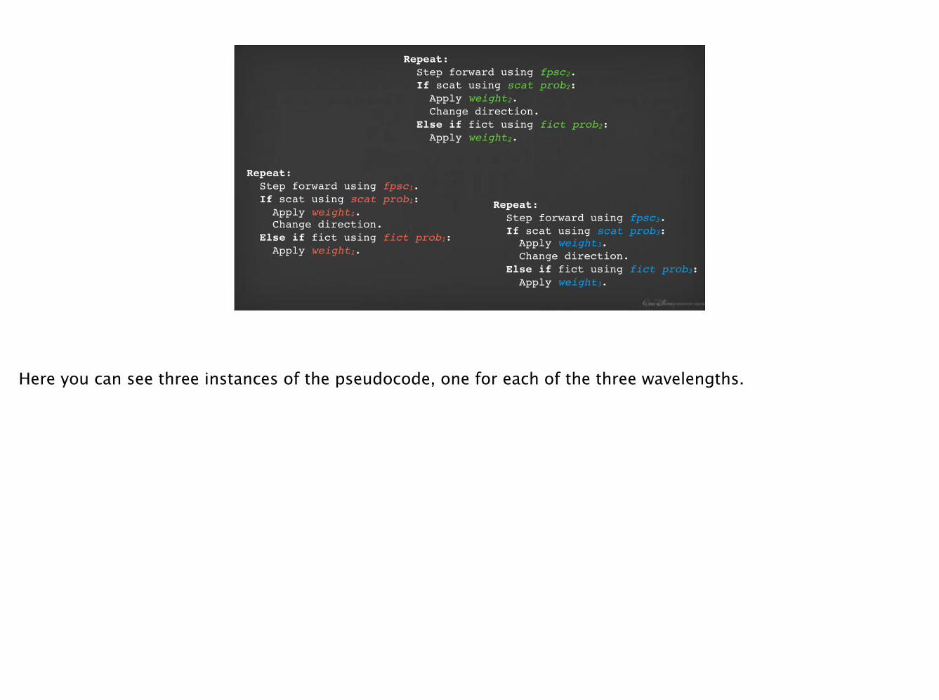
How does spectral tracking work? Here’s an abbreviated version of that weighted-delta-tracking pseudocode from before. Again, the basic way to render three different wavelengths is to trace three separate paths:

Repeat: Step forward using fpsc3. If scat using scat prob3: Apply weight3. Change direction. Else if fict using fict prob3: Apply weight3.

Repeat: Step forward using fpsc2. If scat using scat prob2: Apply weight2. Change direction. Else if fict using fict prob2: Apply weight2.

Repeat: Step forward using fpsc1. If scat using scat prob1: Apply weight1. Change direction. Else if fict using fict prob1: Apply weight1.

Repeat: Step forward using fpsc3. If scat using scat prob3: Apply weight3. Change direction. Else if fict using fict prob3: Apply weight3.

Repeat: Step forward using fpsc2. If scat using scat prob2: Apply weight2. Change direction. Else if fict using fict prob2: Apply weight2.

Repeat: Step forward using fpsc1. If scat using scat prob1: Apply weight1. Change direction. Else if fict using fict prob1: Apply weight1.

Here you can see three instances of the pseudocode, one for each of the three wavelengths.

Repeat: Step forward using fpsc. If scat using scat prob: Apply weight3. Change direction. Else if fict using fict prob: Apply weight3.

Repeat: Step forward using fpsc. If scat using scat prob: Apply weight2. Change direction. Else if fict using fict prob: Apply weight2.

Repeat: Step forward using fpsc. If scat using scat prob: Apply weight1. Change direction. Else if fict using fict prob: Apply weight1.

Some of the variables are flexible, so we can set them to the same thing for each of the wavelengths.

Repeat: Step forward using fpsc. If scat using scat prob: Apply weight3. Change direction. Else if fict using fict prob: Apply weight3.

Repeat: Step forward using fpsc. If scat using scat prob: Apply weight2. Change direction. Else if fict using fict prob: Apply weight2.

Repeat: Step forward using fpsc. If scat using scat prob: Apply weight1. Change direction. Else if fict using fict prob: Apply weight1.

The weights are then really the only thing that differ for the three wavelengths.

(weight1, weight2, weight3)

So in spectral tracking we vectorize the local collision weights and the resultant path throughput.

Repeat: Step forward using fpsc. If scat using scat prob: Apply (weight1, weight2, weight3). Change direction. Else if fict using fict prob: Apply (weight1, weight2, weight3).

And then trace a single path for all of the wavelengths.

Here’s an example of a volume with wavelength-dependent scattering and absorption.

spectral trackingdelta tracking reference

1x 2.7x

TTUV: 1.46 TTUV: 0.54

These equal-samples renders show that spectral tracking will achieve the same variance as delta tracking 2.7 times faster.

free-path-sampling coefficient absorption/emission probability

scattering probability null probability

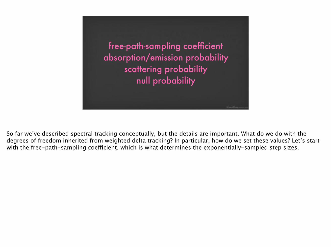
So far we’ve described spectral tracking conceptually, but the details are important. What do we do with the degrees of freedom inherited from weighted delta tracking? In particular, how do we set these values? Let’s start with the free-path-sampling coefficient, which is what determines the exponentially-sampled step sizes.

free-path-sampling coefficient absorption/emission probability

scattering probability null probability

?

So far we’ve described spectral tracking conceptually, but the details are important. What do we do with the degrees of freedom inherited from weighted delta tracking? In particular, how do we set these values? Let’s start with the free-path-sampling coefficient, which is what determines the exponentially-sampled step sizes.

bounding non-bounding non-bounding negated

This can be set to virtually anything, but it should ideally be set to bound the maximum value of the extinction coefficient along the ray over all of the wavelengths being traced. Otherwise exploding and oscillating throughputs can occur, especially if the maximum extinction is severely underestimated. However, it’s worth noting that the algorithm remains unbiased regardless.

free-path-sampling coefficient absorption/emission probability

scattering probability null probability

How about the interaction probabilities? This isn’t as straightforward.

free-path-sampling coefficient absorption/emission probability

scattering probability null probability?

How about the interaction probabilities? This isn’t as straightforward.

delta history-aware max

history-aware average referencemax average

Different probability schemes produce very different noise characteristics, and most of them are vulnerable to high weights and fireflies. The four images in the middle were generated using four of the most interesting possibilities that we investigated. You can see that the right two, history-aware max and history-aware average, both look the least noisy and pretty similar.

delta history-aware max

history-aware average referencemax average

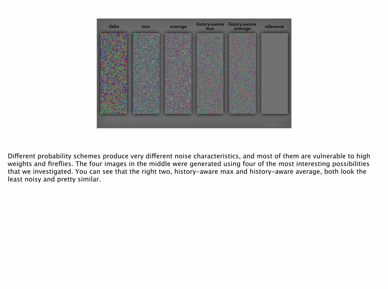
Different probability schemes produce very different noise characteristics, and most of them are vulnerable to high weights and fireflies. The four images in the middle were generated using four of the most interesting possibilities that we investigated. You can see that the right two, history-aware max and history-aware average, both look the least noisy and pretty similar.

delta history-aware max

history-aware average referencemax average

Different probability schemes produce very different noise characteristics, and most of them are vulnerable to high weights and fireflies. The four images in the middle were generated using four of the most interesting possibilities that we investigated. You can see that the right two, history-aware max and history-aware average, both look the least noisy and pretty similar.

history-aware max history-aware average

clos

e-up

with

low

er e

xpos

ure

It’s only in more extreme cases that it becomes clear which one is more robust. This is a volume with wavelength-dependent scattering and no absorption. These images (and all the other images in this talk) were rendered with unlimited multiple scattering. Here you can see that the history-aware-max scheme results in some fireflies whereas the history-aware-average scheme results in none.

1

distance

weight

In general, since we can’t perfectly importance sample all wavelengths simultaneously, the local weight can be above one, and we can experience exponential growth of the path throughput after multiple bounces. This can produce arbitrarily bright fireflies.

1

distance

weight

In general, since we can’t perfectly importance sample all wavelengths simultaneously, the local weight can be above one, and we can experience exponential growth of the path throughput after multiple bounces. This can produce arbitrarily bright fireflies.

1

3

distance

weight

History-Aware-Average Probabilities

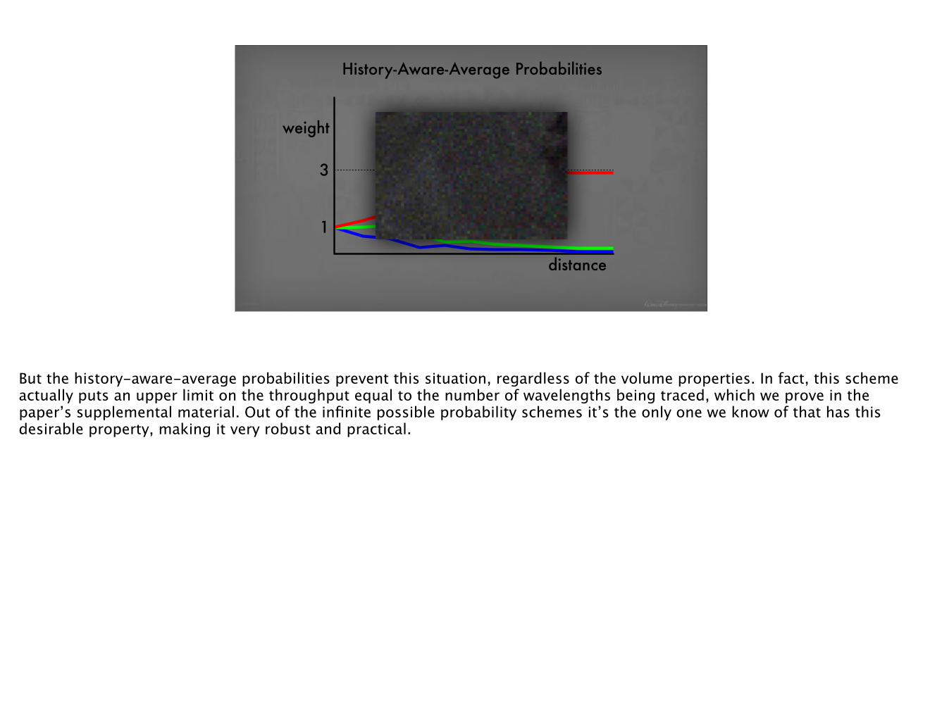
But the history-aware-average probabilities prevent this situation, regardless of the volume properties. In fact, this scheme actually puts an upper limit on the throughput equal to the number of wavelengths being traced, which we prove in the paper’s supplemental material. Out of the infinite possible probability schemes it’s the only one we know of that has this desirable property, making it very robust and practical.

1

3

distance

weight

History-Aware-Average Probabilities

But the history-aware-average probabilities prevent this situation, regardless of the volume properties. In fact, this scheme actually puts an upper limit on the throughput equal to the number of wavelengths being traced, which we prove in the paper’s supplemental material. Out of the infinite possible probability schemes it’s the only one we know of that has this desirable property, making it very robust and practical.

1

3

distance

weight

History-Aware-Average Probabilities

It’s worth noting that in practice, for less extremely chromatic volumes, the throughput for the wavelengths doesn’t diverge as quickly and the path can be shared more equally among the wavelengths.

Putting It All Together

As described by Galtier just last year, the integral formulation that we looked at before can be extended to include multiple components. This allows us to formulate both our decomposition and spectral tracking algorithms in one unifying framework.

As described by Galtier just last year, the integral formulation that we looked at before can be extended to include multiple components. This allows us to formulate both our decomposition and spectral tracking algorithms in one framework.

1x

delta spectral spectral+decomp reference

3.4x 4.1x

TTUV: 1.17 TTUV: 0.35 TTUV: 0.28dragon model source: Stanford University Computer Graphics Laboratory (vripped reconstruction)

Rendering this procedurally subsurface-scattering dragon with both techniques together produces less noise in less time than delta tracking each color channel separately. In this case, spectral and decomposition tracking will achieve the same variance over 4 times faster. Our algorithms are easy to implement, especially if you’re already using delta tracking, so we encourage you to give them a try. We hope that, in the future, others also use the integral framework to derive other novel and useful algorithms, and to transfer ideas between different fields of study. We’re going to leave you with some pretty pictures, but otherwise that concludes this presentation.

[Speech that went along with this video at the Technical Papers Fast Forward: “We introduce two, new, distance-sampling algorithms for more efficient unbiased rendering of chromatic, heterogeneous volumes such as these: spectral tracking for reducing noise and decomposition tracking for reducing render times.”]

[Speech that went along with this video at the Technical Papers Fast Forward: “We introduce two, new, distance-sampling algorithms for more efficient unbiased rendering of chromatic, heterogeneous volumes such as these: spectral tracking for reducing noise and decomposition tracking for reducing render times.”]

This cloud model available soon on disneyanimation.com