Spectral Analysis and Time Series - Max Planck Society · PDF fileA. Lagg – Spectral...
66
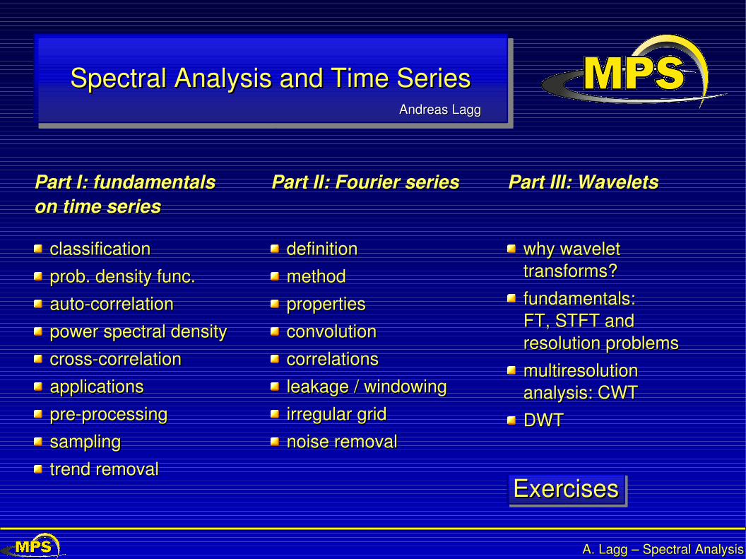
A. Lagg – Spectral Analysis A. Lagg – Spectral Analysis Spectral Analysis and Time Series Spectral Analysis and Time Series Andreas Lagg Andreas Lagg Part I: fundamentals Part I: fundamentals on time series on time series classification classification prob. density func. prob. density func. auto-correlation auto-correlation power spectral density power spectral density cross-correlation cross-correlation applications applications pre-processing pre-processing sampling sampling trend removal trend removal Part II: Fourier series Part II: Fourier series definition definition method method properties properties convolution convolution correlations correlations leakage / windowing leakage / windowing irregular grid irregular grid noise removal noise removal Part III: Wavelets Part III: Wavelets why wavelet why wavelet transforms? transforms? fundamentals: fundamentals: FT, STFT and FT, STFT and resolution problems resolution problems multiresolution multiresolution analysis: CWT analysis: CWT DWT DWT Exercises Exercises
-
Upload
truongthuy -
Category
Documents
-
view
239 -
download
1
Transcript of Spectral Analysis and Time Series - Max Planck Society · PDF fileA. Lagg – Spectral...
A. Lagg – Spectral AnalysisA. Lagg – Spectral Analysis
Spectral Analysis and Time SeriesSpectral Analysis and Time SeriesAndreas LaggAndreas Lagg
Part I: fundamentals Part I: fundamentals on time serieson time series
classificationclassification
prob. density func.prob. density func.
autocorrelationautocorrelation
power spectral densitypower spectral density
crosscorrelationcrosscorrelation
applicationsapplications
preprocessingpreprocessing
samplingsampling
trend removaltrend removal
Part II: Fourier seriesPart II: Fourier series
definitiondefinition
methodmethod
propertiesproperties
convolutionconvolution
correlationscorrelations
leakage / windowingleakage / windowing
irregular gridirregular grid
noise removalnoise removal
Part III: WaveletsPart III: Wavelets
why wavelet why wavelet transforms?transforms?
fundamentals:fundamentals:FT, STFT and FT, STFT and resolution problemsresolution problems
multiresolution multiresolution analysis: CWTanalysis: CWT
DWTDWT
ExercisesExercises

A. Lagg – Spectral AnalysisA. Lagg – Spectral Analysis
Basic description of physical dataBasic description of physical data
deterministic: described by explicit mathematical relationdeterministic: described by explicit mathematical relation
x t =X cos kt
t
nnoonn ddeetteerrmmiinniissttiicc
non deterministic: no way to predict an exact value at a future instant of timenon deterministic: no way to predict an exact value at a future instant of time

A. Lagg – Spectral AnalysisA. Lagg – Spectral Analysis
Classifications of deterministic dataClassifications of deterministic data
PeriodicPeriodic
DeterministicDeterministic
TransientTransientAlmost periodicAlmost periodicComplex PeriodicComplex PeriodicSinusoidalSinusoidal
NonperiodicNonperiodic
A. Lagg – Spectral AnalysisA. Lagg – Spectral Analysis
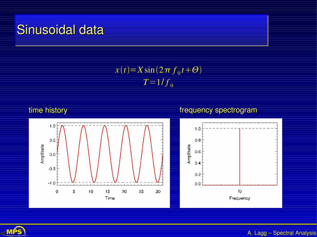
Sinusoidal dataSinusoidal data
x t =X sin 2 f 0 tT=1/ f 0
time historytime history frequency spectrogramfrequency spectrogram

A. Lagg – Spectral AnalysisA. Lagg – Spectral Analysis
Complex periodic dataComplex periodic data
x t =x t±nT n=1,2,3,. ..
x t =a0
2 ∑ an cos 2n f 1 t bn sin 2n f 1 t
time historytime history frequency spectrogramfrequency spectrogram
(T = fundamental period)(T = fundamental period)
A. Lagg – Spectral AnalysisA. Lagg – Spectral Analysis
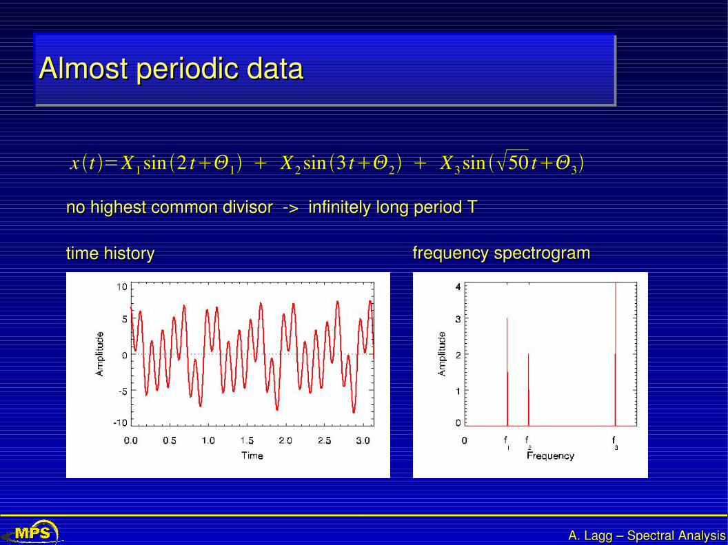
Almost periodic dataAlmost periodic data
x t =X1sin 2 t1 X 2 sin 3 t2 X3 sin 50 t3
time historytime history frequency spectrogramfrequency spectrogram
no highest common divisor > infinitely long period Tno highest common divisor > infinitely long period T

A. Lagg – Spectral AnalysisA. Lagg – Spectral Analysis
Transient nonperiodic dataTransient nonperiodic data
x t ={ A c≥t≥00 ct0
all nonperiodic data other than almost periodic dataall nonperiodic data other than almost periodic data
x t ={ Ae−at t≥00 t0
x t ={ Ae−at cos bt t≥00 t0

A. Lagg – Spectral AnalysisA. Lagg – Spectral Analysis
Classification of random dataClassification of random data
StationaryStationary
Random DataRandom Data
Special classificationsSpecial classifications
of nonstationarityof nonstationarity
NonergodicNonergodicErgodicErgodic
NonstationaryNonstationary

A. Lagg – Spectral AnalysisA. Lagg – Spectral Analysis
stationary / non stationarystationary / non stationary
collection of sample functions = ensemblecollection of sample functions = ensemble
autocorrelation function (joint moment):autocorrelation function (joint moment):
Rx t1, t1= limN ∞
1N ∑
k=1
N
xk t1 xk t1
mean value (first moment):mean value (first moment):
x t1= limN ∞
1N ∑
k=1
N
xk t1
stationary: stationary: x t1=x , Rx t1, t1=Rx
data can be (hypothetically) described by data can be (hypothetically) described by computing ensemble averages (averaging over computing ensemble averages (averaging over multiple measurements / sample functions)multiple measurements / sample functions)
weakly stationary: weakly stationary: x t1=x , Rx t1, t1=Rx
A. Lagg – Spectral AnalysisA. Lagg – Spectral Analysis
ergodic / non ergodicergodic / non ergodic
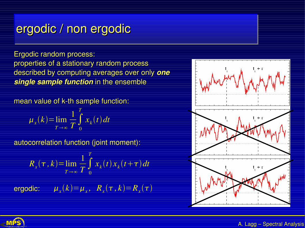
Ergodic random process:Ergodic random process:properties of a stationary random process properties of a stationary random process described by computing averages over only described by computing averages over only one one single sample functionsingle sample function in the ensemble in the ensemble
autocorrelation function (joint moment):autocorrelation function (joint moment):
Rx , k = limT ∞
1T ∫
0
T
xk t xk tdt
mean value of kth sample function:mean value of kth sample function:
x k = limT ∞
1T ∫
0
T
xk t dt
ergodic: ergodic: x k =x , Rx , k =Rx
A. Lagg – Spectral AnalysisA. Lagg – Spectral Analysis
Basic descriptive properties of random dataBasic descriptive properties of random data
mean square valuesmean square values
propability density functionpropability density function
autocorrelation functionsautocorrelation functions
power spectral density functionspower spectral density functions
(from now on: assume random data to be stationary and ergodic)(from now on: assume random data to be stationary and ergodic)
A. Lagg – Spectral AnalysisA. Lagg – Spectral Analysis
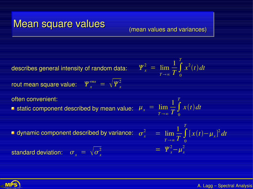
Mean square valuesMean square values(mean values and variances)(mean values and variances)
describes general intensity of random data:describes general intensity of random data: x2 = lim
T ∞
1T ∫
0
T
x2t dt
rout mean square value: rout mean square value: xrms = x
2
often convenient:often convenient:
static component described by mean value:static component described by mean value:
dynamic component described by variance:dynamic component described by variance:
x = limT ∞
1T ∫
0
T
x t dt
x2 = lim
T ∞
1T ∫
0
T
[ x t −x ]2 dt
= x2−x
2
standard deviation: standard deviation: x = x2
A. Lagg – Spectral AnalysisA. Lagg – Spectral Analysis
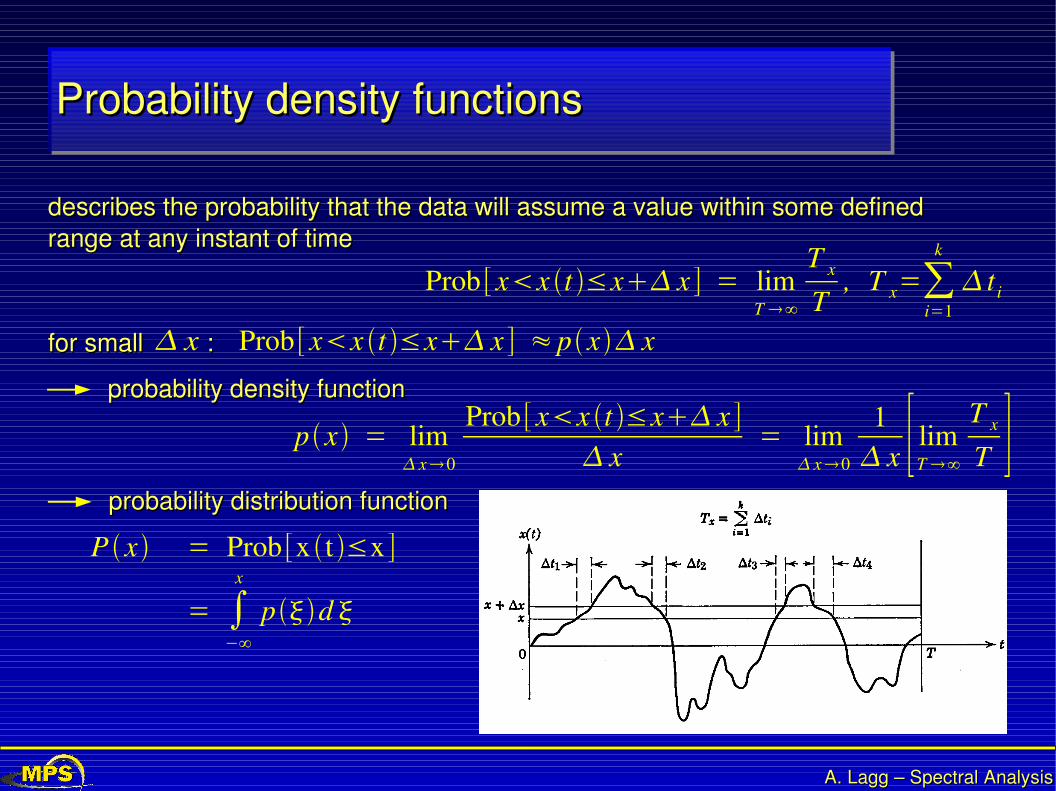
Probability density functionsProbability density functions
describes the probability that the data will assume a value within some defined describes the probability that the data will assume a value within some defined range at any instant of timerange at any instant of time
Prob [ xx t ≤x x ] = limT ∞
T x
T, T x=∑
i=1
k
t i
for small :for small : x Prob [ xx t ≤x x ] ≈ px x
px = lim x0
Prob [ xx t ≤x x ] x
= lim x0
1 x [ lim
T ∞
T x
T ]probability density functionprobability density function
probability distribution functionprobability distribution function
P x = Prob [x t ≤x ]
= ∫−∞
x
pd

A. Lagg – Spectral AnalysisA. Lagg – Spectral Analysis
Illustration: probability density functionIllustration: probability density function
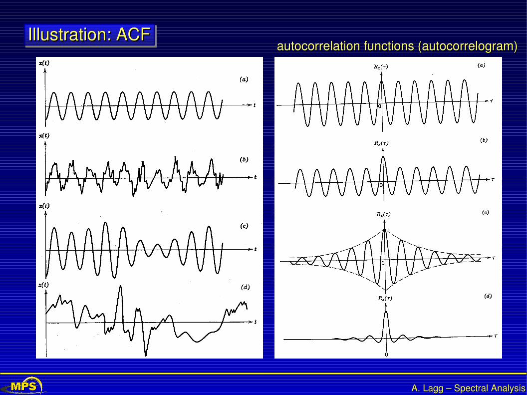
sample time histories:sample time histories:
sine wave (a)sine wave (a)
sine wave + random noisesine wave + random noise
narrowband random noisenarrowband random noise
wideband random noisewideband random noise
all 4 cases: mean valueall 4 cases: mean value x=0

A. Lagg – Spectral AnalysisA. Lagg – Spectral Analysis
Illustration: probability density functionIllustration: probability density functionprobability density functionprobability density function

A. Lagg – Spectral AnalysisA. Lagg – Spectral Analysis
Autocorrelation functionsAutocorrelation functions
describes the general dependence of the data values at one time on the describes the general dependence of the data values at one time on the values at another time.values at another time.
Rx = limT ∞
1T ∫
0
T
x t x tdt
x = Rx ∞ x2 = Rx 0 (not for special cases like sine waves)(not for special cases like sine waves)
A. Lagg – Spectral AnalysisA. Lagg – Spectral Analysis
Illustration: ACFIllustration: ACFautocorrelation functions (autocorrelogram)autocorrelation functions (autocorrelogram)
A. Lagg – Spectral AnalysisA. Lagg – Spectral Analysis
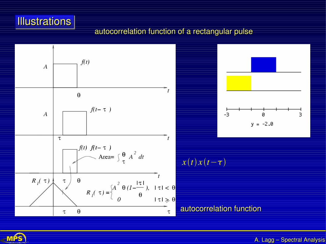
IllustrationsIllustrations
autocorrelation functionautocorrelation function
x t x t−
autocorrelation function of a rectangular pulseautocorrelation function of a rectangular pulse
A. Lagg – Spectral AnalysisA. Lagg – Spectral Analysis
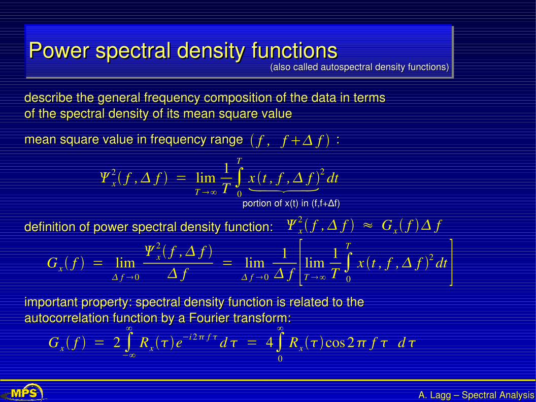
Power spectral density functionsPower spectral density functions(also called autospectral density functions)(also called autospectral density functions)
describe the general frequency composition of the data in terms describe the general frequency composition of the data in terms of the spectral density of its mean square valueof the spectral density of its mean square value
mean square value in frequency range :mean square value in frequency range : f , f f
x2 f , f = lim
T ∞
1T ∫
0
T
x t , f , f 2 dt
portion of x(t) in (f,f+portion of x(t) in (f,f+∆∆f)f)
x2 f , f ≈ G x f fdefinition of power spectral density function:definition of power spectral density function:
G x f = lim f 0
x2 f , f f
= lim f 0
1 f [ lim
T ∞
1T ∫
0
T
x t , f , f 2 dt ]important property: spectral density function is related to the important property: spectral density function is related to the autocorrelation function by a Fourier transform:autocorrelation function by a Fourier transform:
G x f = 2∫−∞
∞
Rx e−i 2 f d = 4∫0
∞
Rx cos 2 f d

A. Lagg – Spectral AnalysisA. Lagg – Spectral Analysis
Illustration: PSDIllustration: PSD
sine wavesine wave
broadbandbroadbandnoisenoise
narrowbandnarrowbandnoisenoise
sine wavesine wave+ random noise+ random noise
power spectral density functionspower spectral density functions
Dirac delta function at f=fDirac delta function at f=f00
““white” noise:white” noise:spectrum is uniform over spectrum is uniform over all frequenciesall frequencies
A. Lagg – Spectral AnalysisA. Lagg – Spectral Analysis
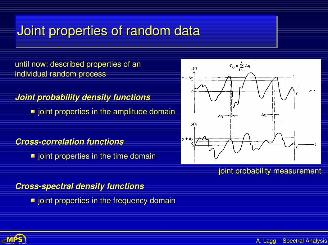
Joint properties of random dataJoint properties of random data
Joint probability density functionsJoint probability density functions
joint properties in the amplitude domainjoint properties in the amplitude domain
Crossspectral density functionsCrossspectral density functions
joint properties in the frequency domainjoint properties in the frequency domain
Crosscorrelation functionsCrosscorrelation functions
joint properties in the time domainjoint properties in the time domain
joint probability measurementjoint probability measurement
until now: described properties of an until now: described properties of an individual random process individual random process
A. Lagg – Spectral AnalysisA. Lagg – Spectral Analysis
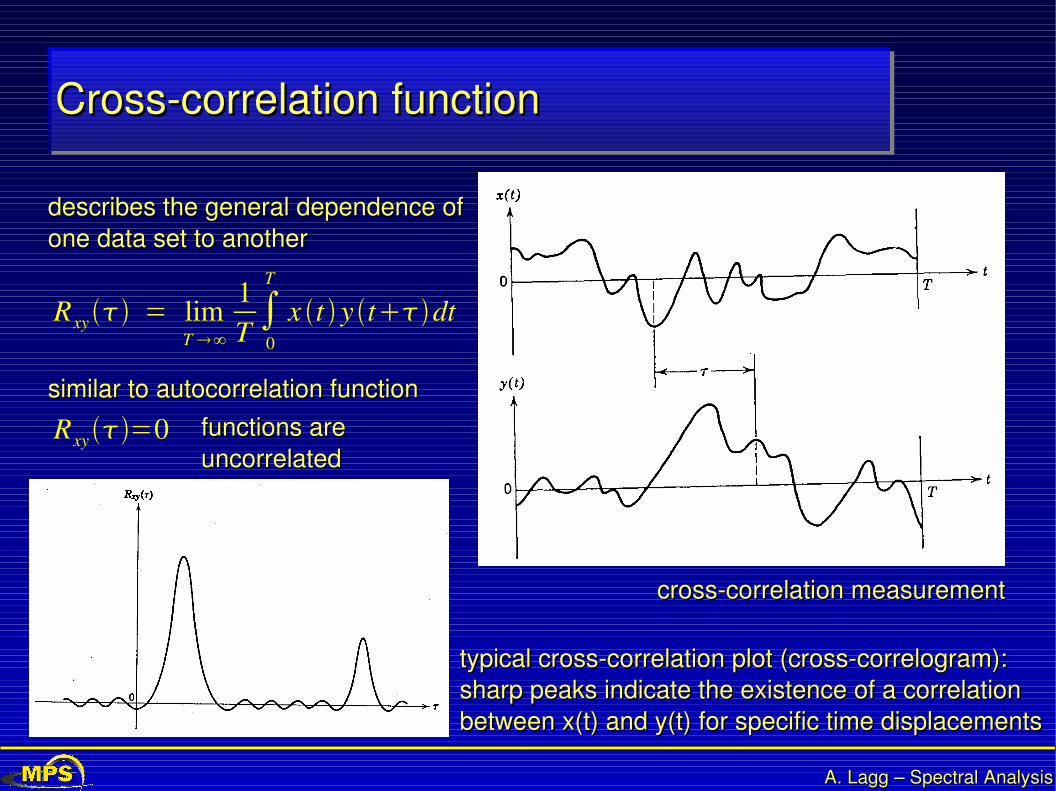
Crosscorrelation functionCrosscorrelation function
crosscorrelation measurementcrosscorrelation measurement
describes the general dependence of describes the general dependence of one data set to anotherone data set to another
Rxy = limT ∞
1T ∫
0
T
x t y tdt
similar to autocorrelation functionsimilar to autocorrelation function
Rxy=0 functions are functions are uncorrelateduncorrelated
typical crosscorrelation plot (crosscorrelogram):typical crosscorrelation plot (crosscorrelogram):sharp peaks indicate the existence of a correlation sharp peaks indicate the existence of a correlation between x(t) and y(t) for specific time displacementsbetween x(t) and y(t) for specific time displacements

A. Lagg – Spectral AnalysisA. Lagg – Spectral Analysis
ApplicationsApplications
Measurement of time delaysMeasurement of time delays
2 signals:2 signals:
different offsetdifferent offset
different S/Ndifferent S/N
time delay 4stime delay 4s
often used:often used:'discrete' cross correlation coefficient'discrete' cross correlation coefficientlag =l, for l >=0:lag =l, for l >=0:
Rxyl =∑k=1
N−l
xk−x ykl−y
∑k=1
N
xk−x2∑k=1
N
yk−y2

A. Lagg – Spectral AnalysisA. Lagg – Spectral Analysis
ApplicationsApplicationsDetection and recovery from Detection and recovery from signals in noisesignals in noise
3 signals:3 signals:
noise free replica of the signal noise free replica of the signal (e.g. model)(e.g. model)
2 noisy signals2 noisy signals
cross correlation can be used to cross correlation can be used to determine if theoretical signal is determine if theoretical signal is present in datapresent in data
A. Lagg – Spectral AnalysisA. Lagg – Spectral Analysis
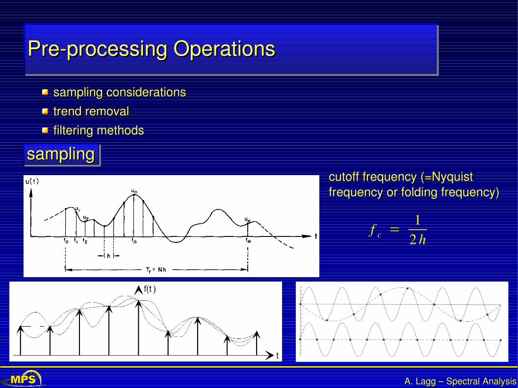
Preprocessing OperationsPreprocessing Operations
sampling considerationssampling considerations
trend removaltrend removal
filtering methodsfiltering methods
samplingsamplingcutoff frequency (=Nyquist cutoff frequency (=Nyquist frequency or folding frequency)frequency or folding frequency)
f c =1
2 h
A. Lagg – Spectral AnalysisA. Lagg – Spectral Analysis
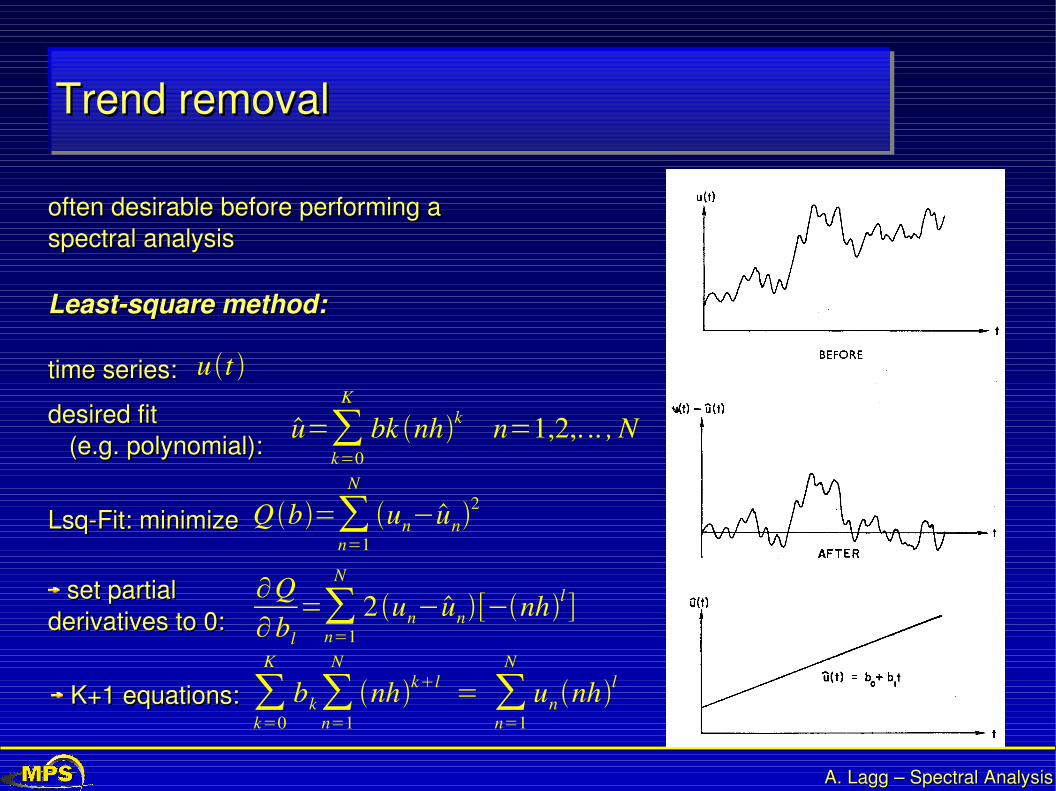
Trend removalTrend removal
often desirable before performing a often desirable before performing a spectral analysisspectral analysis
Leastsquare method:Leastsquare method:
time series: time series: ut
desired fitdesired fit (e.g. polynomial): (e.g. polynomial):
u=∑k=0
K
bk nhk n=1,2,. .. , N
LsqFit: minimize LsqFit: minimize Qb=∑n=1
N
un−un2
set partialset partialderivatives to 0: derivatives to 0:
∂Q∂bl
=∑n=1
N
2 un−un[−nhl ]
K+1 equations:K+1 equations: ∑k=0
K
bk∑n=1
N
nhkl = ∑n=1
N
unnhl
A. Lagg – Spectral AnalysisA. Lagg – Spectral Analysis
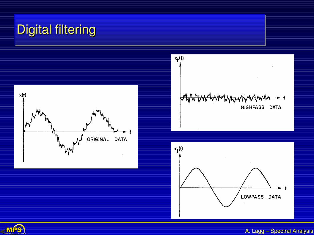
Digital filteringDigital filtering
A. Lagg – Spectral AnalysisA. Lagg – Spectral Analysis
end of part I ...end of part I ...

A. Lagg – Spectral AnalysisA. Lagg – Spectral Analysis
Spectral Analysis and Time SeriesSpectral Analysis and Time SeriesAndreas LaggAndreas Lagg
Part I: fundamentals Part I: fundamentals on time serieson time series
classificationclassification
prob. density func.prob. density func.
autocorrelationautocorrelation
power spectral densitypower spectral density
crosscorrelationcrosscorrelation
applicationsapplications
preprocessingpreprocessing
samplingsampling
trend removaltrend removal
Part II: Fourier seriesPart II: Fourier series
definitiondefinition
methodmethod
propertiesproperties
convolutionconvolution
correlationscorrelations
leakage / windowingleakage / windowing
irregular gridirregular grid
noise removalnoise removal
Part III: WaveletsPart III: Wavelets
why wavelet why wavelet transforms?transforms?
fundamentals:fundamentals:FT, STFT and FT, STFT and resolution problemsresolution problems
multiresolution multiresolution analysis: CWTanalysis: CWT
DWTDWT
ExercisesExercises
A. Lagg – Spectral AnalysisA. Lagg – Spectral Analysis
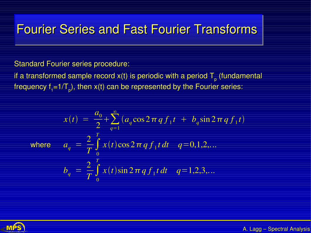
Fourier Series and Fast Fourier TransformsFourier Series and Fast Fourier Transforms
Standard Fourier series procedure:Standard Fourier series procedure:
if a transformed sample record x(t) is periodic with a period Tif a transformed sample record x(t) is periodic with a period Tpp (fundamental (fundamental frequency ffrequency f11=1/T=1/Tpp), then x(t) can be represented by the Fourier series:), then x(t) can be represented by the Fourier series:
x t =a0
2∑
q=1
∞
aq cos 2q f 1 t bq sin 2q f 1 t
aq =2T ∫
0
T
x t cos 2q f 1 t dt q=0,1,2,. ..
bq =2T ∫
0
T
x t sin 2q f 1 t dt q=1,2,3,. ..
wherewhere
A. Lagg – Spectral AnalysisA. Lagg – Spectral Analysis
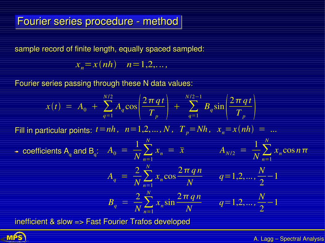
Fourier series procedure methodFourier series procedure method
sample record of finite length, equally spaced sampled:sample record of finite length, equally spaced sampled:
xn=x nh n=1,2,. .. , N
Fourier series passing through these N data values:Fourier series passing through these N data values:
x t = A0 ∑q=1
N /2
Aq cos 2q tT p
∑q=1
N /2−1
Bq sin 2q tT p
Fill in particular points:Fill in particular points: t=nh , n=1,2, ... , N , T p=Nh , xn=x nh = ...
coefficients Acoefficients Aqq and B and Bqq:: A0 =1N ∑
n=1
N
xn = x AN /2 =1N ∑
n=1
N
xn cos n
Aq =2N ∑
n=1
N
xn cos2q n
Nq=1,2, ... ,
N2
−1
Bq =2N ∑
n=1
N
xn sin2q n
Nq=1,2, ... ,
N2
−1
inefficient & slow => Fast Fourier Trafos developedinefficient & slow => Fast Fourier Trafos developed
A. Lagg – Spectral AnalysisA. Lagg – Spectral Analysis
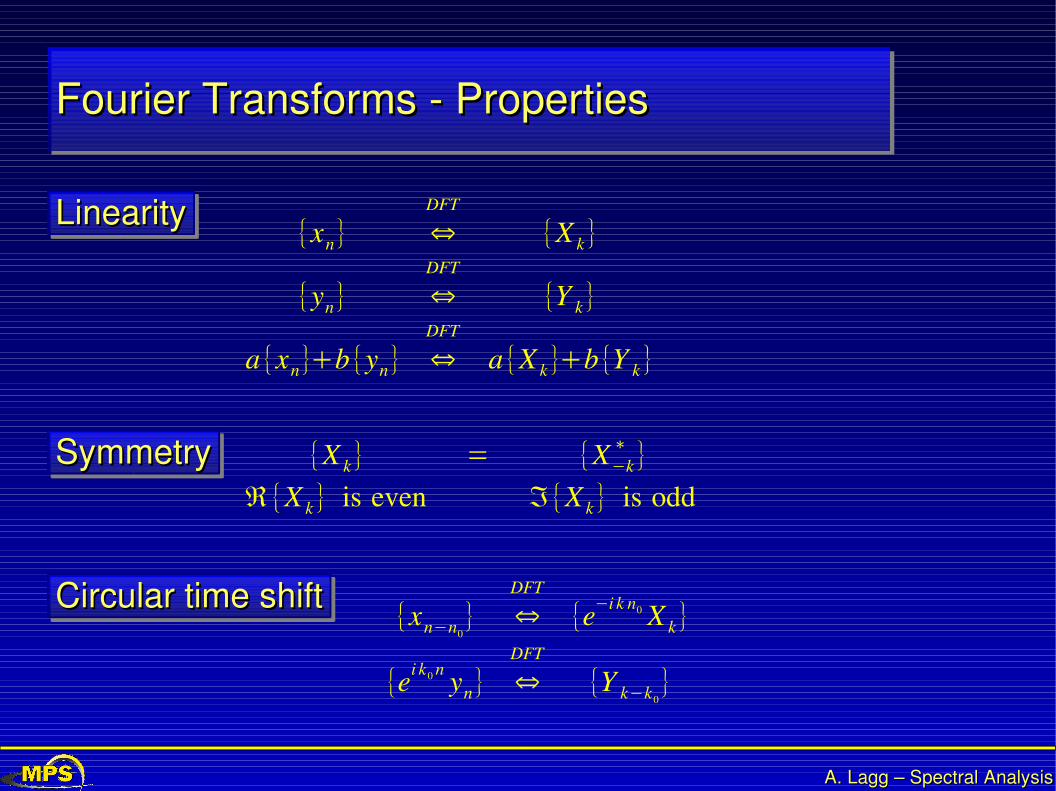
Fourier Transforms PropertiesFourier Transforms Properties
LinearityLinearity
{xn−n0} ⇔
DFT
{e−i k n0 X k}
{ei k0 n yn} ⇔DFT
{Y k−k0}
SymmetrySymmetry {X k} = {X−k∗ }
ℜ{X k} is even ℑ{X k} is odd
Circular time shiftCircular time shift
{xn} ⇔DFT
{X k}
{yn} ⇔DFT
{Y k}
a {xn}b {yn} ⇔DFT
a {X k}b{Y k}

A. Lagg – Spectral AnalysisA. Lagg – Spectral Analysis
Using FFT for ConvolutionUsing FFT for Convolution
Convolution Theorem:Convolution Theorem:
r * s ≡ ∫−∞
∞
r s t−d
r * s ⇔FT
R f S f
Fourier transform of the convolution Fourier transform of the convolution is product of the individual Fourier is product of the individual Fourier transformstransforms
(note how the response function for negative times is wrapped (note how the response function for negative times is wrapped around and stored at the extreme right end of the array)around and stored at the extreme right end of the array)
discrete case:discrete case:
r * s j ≡ ∑k=−N /21
N /2
s j−k r k
∑k=−N /21
N /2
s j−k r k ⇔FT
Rn Sn
Convolution Theorem:Convolution Theorem: constraints:constraints:
duration of r and s are not the sameduration of r and s are not the same
signal is not periodicsignal is not periodic
original dataoriginal data
response functionresponse function
convolved dataconvolved data

A. Lagg – Spectral AnalysisA. Lagg – Spectral Analysis
Treatment of end effects by zero paddingTreatment of end effects by zero padding
constraint 1:constraint 1: simply expand response function to length N by padding it with zerossimply expand response function to length N by padding it with zeros
constraint 2:constraint 2: extend data at one end with a number of zeros equal to the max. extend data at one end with a number of zeros equal to the max. positive / negative duration of r (whichever is larger)positive / negative duration of r (whichever is larger)

A. Lagg – Spectral AnalysisA. Lagg – Spectral Analysis
FFT for ConvolutionFFT for Convolution
1.1. zeropad datazeropad data
2.2. zeropad response functionzeropad response function(> data and response function have N elements)(> data and response function have N elements)
3.3. calculate FFT of data and response functioncalculate FFT of data and response function
4.4. multiply FFT of data with FFT of response functionmultiply FFT of data with FFT of response function
5.5. calculate inverse FFT for this productcalculate inverse FFT for this product
DeconvolutionDeconvolution
> undo smearing caused by a response function> undo smearing caused by a response function
use steps (13), and then:use steps (13), and then:
4.4. divide FFT of convolved data with FFT of response divide FFT of convolved data with FFT of response functionfunction
5.5. calculate inverse FFT for this productcalculate inverse FFT for this product

A. Lagg – Spectral AnalysisA. Lagg – Spectral Analysis
Correlation / Autocorrelation with FFTCorrelation / Autocorrelation with FFT
definition of correlation / autocorrelation see first lecturedefinition of correlation / autocorrelation see first lecture
Corr g , h = g* h = ∫−∞
∞
gth d
Correlation Theorem:Correlation Theorem:
Corr g , h ⇔FT
G f H* f
AutoCorrelation:AutoCorrelation:
Corr g , g ⇔FT
∣G f ∣2
discrete correlation theorem:discrete correlation theorem:
Corr g , h j ≡ ∑k=0
N−1
g jk hk
⇔FT
Gk H k*

A. Lagg – Spectral AnalysisA. Lagg – Spectral Analysis
Fourier Transform problemsFourier Transform problems
spectral leakagespectral leakage
T=nT p T≠nT p
A. Lagg – Spectral AnalysisA. Lagg – Spectral Analysis
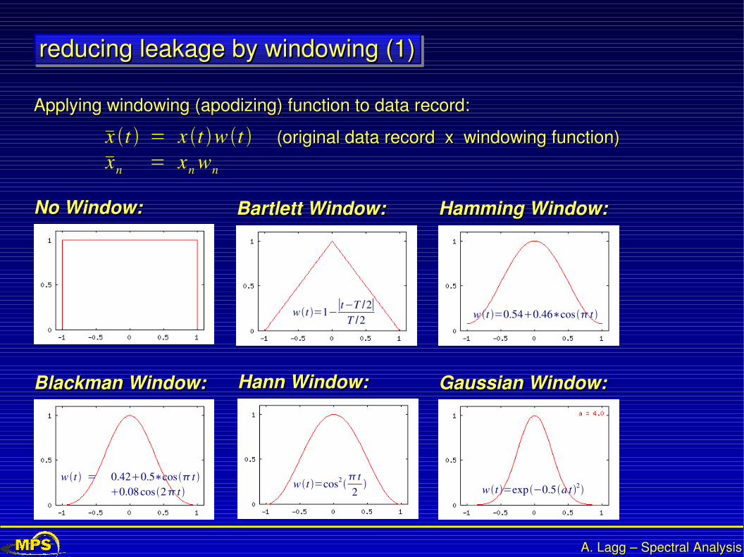
reducing leakage by windowing (1)reducing leakage by windowing (1)
Applying windowing (apodizing) function to data record:Applying windowing (apodizing) function to data record:
x t = x t w t xn = xn wn
(original data record x windowing function)(original data record x windowing function)
No Window:No Window: Bartlett Window:Bartlett Window: Hamming Window:Hamming Window:
Blackman Window:Blackman Window: Hann Window:Hann Window: Gaussian Window:Gaussian Window:
wt =0.540.46∗cos t
wt = 0.420.5∗cos t 0.08 cos2 t
wt =cos2 t2
wt =exp −0.5a t 2
wt =1−∣t−T /2∣
T /2
A. Lagg – Spectral AnalysisA. Lagg – Spectral Analysis
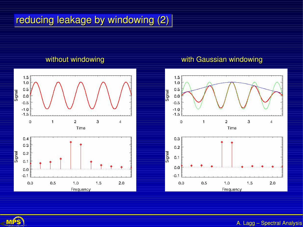
reducing leakage by windowing (2)reducing leakage by windowing (2)
without windowingwithout windowing with Gaussian windowingwith Gaussian windowing
A. Lagg – Spectral AnalysisA. Lagg – Spectral Analysis
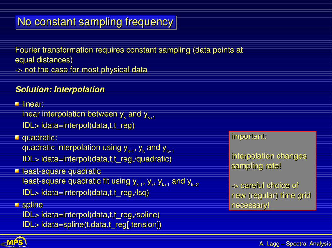
No constant sampling frequencyNo constant sampling frequency
Fourier transformation requires constant sampling (data points at Fourier transformation requires constant sampling (data points at equal distances)equal distances)> not the case for most physical data> not the case for most physical data
Solution: InterpolationSolution: Interpolation
linear:linear:inear interpolation between yinear interpolation between ykk and y and yk+1k+1
IDL> idata=interpol(data,t,t_reg)IDL> idata=interpol(data,t,t_reg)
quadratic:quadratic:quadratic interpolation using yquadratic interpolation using yk1k1, y, ykk and y and yk+1k+1
IDL> idata=interpol(data,t,t_reg,/quadratic)IDL> idata=interpol(data,t,t_reg,/quadratic)
leastsquare quadraticleastsquare quadraticleastsquare quadratic fit using yleastsquare quadratic fit using yk1k1, y, ykk, y, yk+1k+1 and y and yk+2k+2
IDL> idata=interpol(data,t,t_reg,/lsq)IDL> idata=interpol(data,t,t_reg,/lsq)
splinesplineIDL> idata=interpol(data,t,t_reg,/spline)IDL> idata=interpol(data,t,t_reg,/spline)IDL> idata=spline(t,data,t_reg[,tension])IDL> idata=spline(t,data,t_reg[,tension])
important:important:
interpolation changes interpolation changes sampling rate!sampling rate!
> careful choice of > careful choice of new (regular) time grid new (regular) time grid necessary!necessary!

A. Lagg – Spectral AnalysisA. Lagg – Spectral Analysis
Fourier Transorm on irregular gridded data InterpolationFourier Transorm on irregular gridded data Interpolation
original data: sine wave + noiseoriginal data: sine wave + noise
FT of original dataFT of original data
irregular sampling of data (measurement)irregular sampling of data (measurement)
interpolation: linear, lsq, spline, quadraticinterpolation: linear, lsq, spline, quadratic'resampling' 'resampling'
FT of interpolated dataFT of interpolated data
A. Lagg – Spectral AnalysisA. Lagg – Spectral Analysis
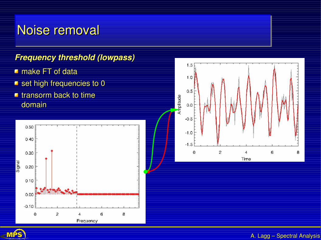
Noise removalNoise removal
Frequency threshold (lowpass)Frequency threshold (lowpass)
make FT of datamake FT of data
set high frequencies to 0set high frequencies to 0
transorm back to time transorm back to time domaindomain

A. Lagg – Spectral AnalysisA. Lagg – Spectral Analysis
Noise removalNoise removal
signal threshold forsignal threshold forweak frequencies (dBthreshold)weak frequencies (dBthreshold)
make FT of datamake FT of data
set frequencies with amplitudes set frequencies with amplitudes below a given threshold to 0below a given threshold to 0
transorm back to time domaintransorm back to time domain
A. Lagg – Spectral AnalysisA. Lagg – Spectral Analysis
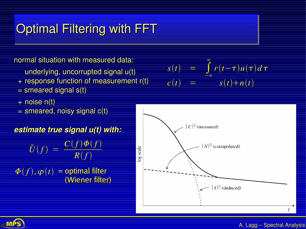
Optimal Filtering with FFTOptimal Filtering with FFT
normal situation with measured data:normal situation with measured data:
underlying, uncorrupted signal u(t)underlying, uncorrupted signal u(t) + + response function of measurement r(t)response function of measurement r(t) = smeared signal s(t) = smeared signal s(t)
++ noise n(t)noise n(t) = = smeared, noisy signal c(t)smeared, noisy signal c(t)
s t = ∫−∞
∞
r t−ud
c t = st nt
estimate true signal u(t) with:estimate true signal u(t) with:
U f =C f f
R f
f ,t = optimal filter = optimal filter (Wiener filter) (Wiener filter)

A. Lagg – Spectral AnalysisA. Lagg – Spectral Analysis
Calculation of optimal filterCalculation of optimal filter
reconstructed signal and uncorrupted signal should be close in leastsquare sense:reconstructed signal and uncorrupted signal should be close in leastsquare sense:> minimize > minimize
∫−∞
∞
∣ut −ut ∣2 dt = ∫−∞
∞
∣ U f −U f ∣2 df
⇒ ∂∂ f ∣[S f N f ] f
R f −
S f R f ∣
2
= 0
⇒ f =∣S f ∣2
∣S f ∣2∣N f ∣2
additional information:additional information:power spectral density can often power spectral density can often be used to disentangle noise be used to disentangle noise function N(f) from smeared function N(f) from smeared signal S(f)signal S(f)

A. Lagg – Spectral AnalysisA. Lagg – Spectral Analysis
Using FFT for Power Spectrum EstimationUsing FFT for Power Spectrum Estimation
PeriodogramPeriodogram
discrete Fourier transform of c(t)discrete Fourier transform of c(t)> Fourier coefficients:> Fourier coefficients:
C k=∑j=0
N−1
c j e2 i j k /N k=0, ... , N−1
> periodogram estimate of > periodogram estimate of power spectrum:power spectrum:
P 0 = P f 0=1
N 2∣C0∣2
P f k =1
N 2 [∣Ck∣2∣C N−k∣
2 ]
P f c = P f N /2=1
N 2∣C N /2∣2

A. Lagg – Spectral AnalysisA. Lagg – Spectral Analysis
end of FTend of FT

A. Lagg – Spectral AnalysisA. Lagg – Spectral Analysis
Spectral Analysis and Time SeriesSpectral Analysis and Time SeriesAndreas LaggAndreas Lagg
Part I: fundamentals Part I: fundamentals on time serieson time series
classificationclassification
prob. density func.prob. density func.
autocorrelationautocorrelation
power spectral densitypower spectral density
crosscorrelationcrosscorrelation
applicationsapplications
preprocessingpreprocessing
samplingsampling
trend removaltrend removal
Part II: Fourier seriesPart II: Fourier series
definitiondefinition
methodmethod
propertiesproperties
convolutionconvolution
correlationscorrelations
leakage / windowingleakage / windowing
irregular gridirregular grid
noise removalnoise removal
Part III: WaveletsPart III: Wavelets
why wavelet why wavelet transforms?transforms?
fundamentals:fundamentals:FT, STFT and FT, STFT and resolution problemsresolution problems
multiresolution multiresolution analysis: CWTanalysis: CWT
DWTDWT
ExercisesExercises

A. Lagg – Spectral AnalysisA. Lagg – Spectral Analysis
Introduction to WaveletsIntroduction to Wavelets
why wavelet transforms?why wavelet transforms?
fundamentals: FT, short term FT and resolution fundamentals: FT, short term FT and resolution problemsproblems
multiresolution analysis:multiresolution analysis:continous wavelet transformcontinous wavelet transform
multiresolution analysis:multiresolution analysis:discrete wavelet transformdiscrete wavelet transform
A. Lagg – Spectral AnalysisA. Lagg – Spectral Analysis
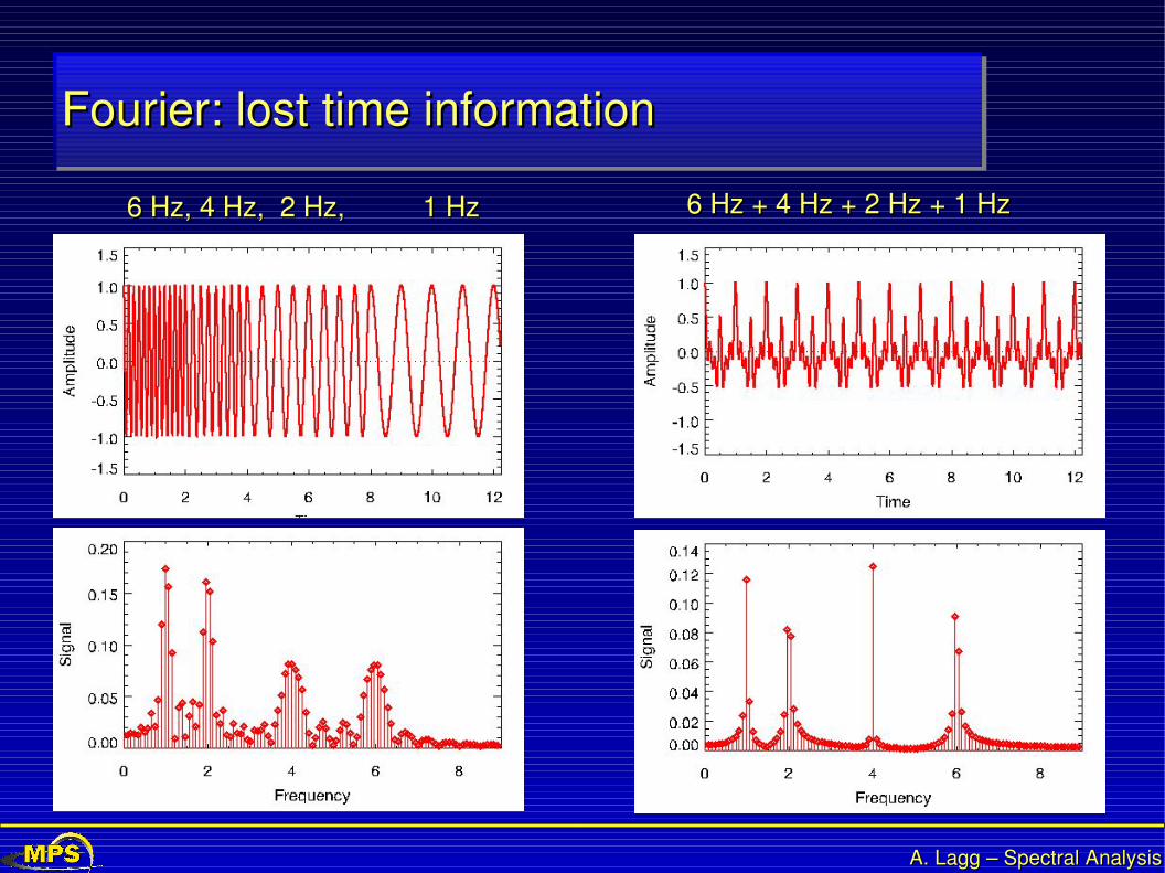
Fourier: lost time informationFourier: lost time information
6 Hz, 4 Hz, 2 Hz, 1 Hz6 Hz, 4 Hz, 2 Hz, 1 Hz 6 Hz + 4 Hz + 2 Hz + 1 Hz6 Hz + 4 Hz + 2 Hz + 1 Hz
A. Lagg – Spectral AnalysisA. Lagg – Spectral Analysis
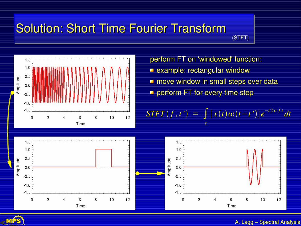
Solution: Short Time Fourier TransformSolution: Short Time Fourier Transform(STFT)(STFT)
perform FT on 'windowed' function:perform FT on 'windowed' function:
example: rectangular windowexample: rectangular window
move window in small steps over datamove window in small steps over data
perform FT for every time stepperform FT for every time step
STFT f , t ' = ∫t
[ x t t−t ' ]e−i 2 f t dt

A. Lagg – Spectral AnalysisA. Lagg – Spectral Analysis
Short Time Fourier TransformShort Time Fourier Transform
STFTSTFT
STFTspectrogram shows both time and STFTspectrogram shows both time and frequency information!frequency information!
A. Lagg – Spectral AnalysisA. Lagg – Spectral Analysis
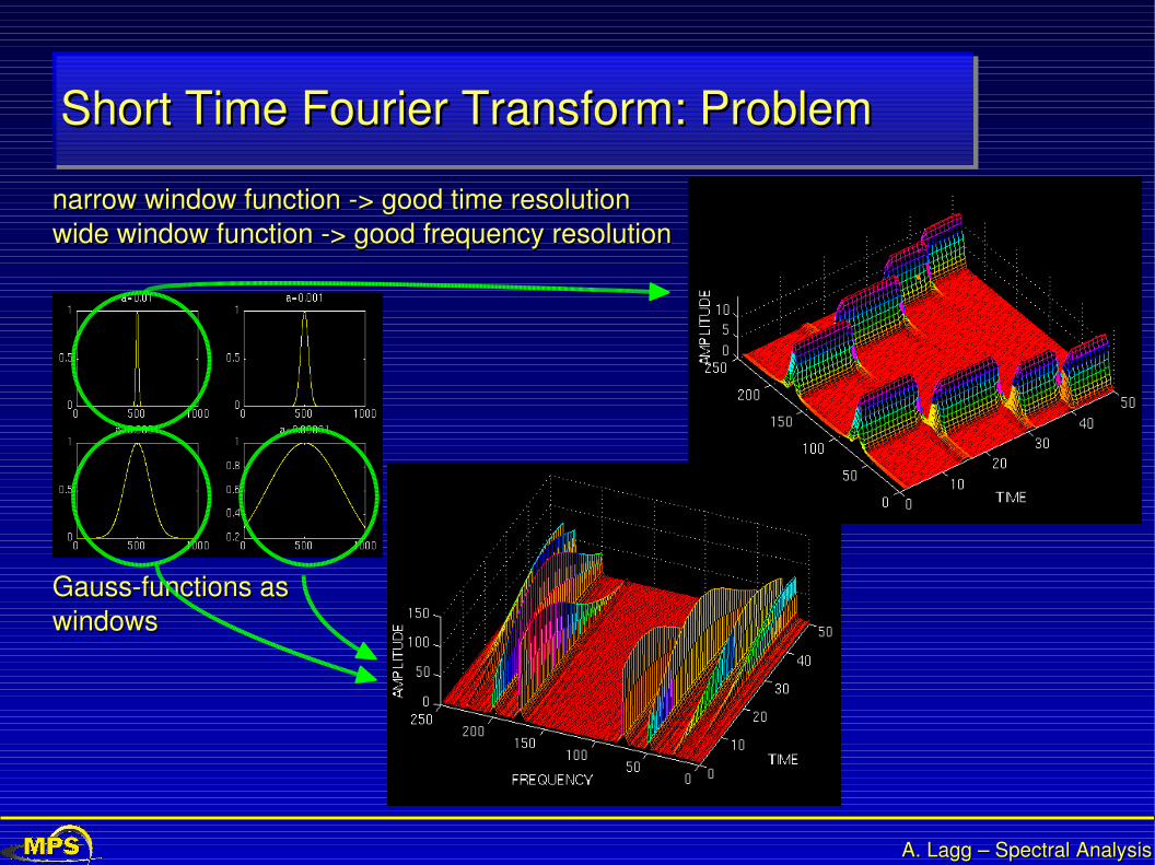
Gaussfunctions as Gaussfunctions as windowswindows
Short Time Fourier Transform: ProblemShort Time Fourier Transform: Problem
narrow window function > good time resolutionnarrow window function > good time resolutionwide window function > good frequency resolutionwide window function > good frequency resolution
A. Lagg – Spectral AnalysisA. Lagg – Spectral Analysis
Solution: Wavelet TransformationSolution: Wavelet Transformation
time vs. frequency resolution is intrinsic problem (Heisenberg Uncertainty Principle)time vs. frequency resolution is intrinsic problem (Heisenberg Uncertainty Principle)approach: analyze the signal at different frequencies with different resolutionsapproach: analyze the signal at different frequencies with different resolutions
> multiresolution analysis (MRA)> multiresolution analysis (MRA)
Continuous Wavelet TransformContinuous Wavelet Transform
similar to STFT:similar to STFT:
signal is multiplied with a signal is multiplied with a function (the function (the waveletwavelet))
transform is calculated transform is calculated separately for different segments separately for different segments of the time domainof the time domain
but:but:
the FT of the windowed signals are the FT of the windowed signals are not takennot taken(no negative frequencies)(no negative frequencies)
The width of the window is changed The width of the window is changed as the transform is computed for as the transform is computed for every single spectral componentevery single spectral component

A. Lagg – Spectral AnalysisA. Lagg – Spectral Analysis
Continuous Wavelet TransformContinuous Wavelet Transform
CWT x =x
, s =1
∣s∣∫t
x t * t−s dt
... translation parameter , s ... scale parameter
t ... mother wavelet = small wave
mother wavelet:mother wavelet:
finite length (compactly finite length (compactly supported) >'let'supported) >'let'
oscillatory >'wave'oscillatory >'wave'
functions for different functions for different regions are derived from regions are derived from this function > 'mother'this function > 'mother'
scale parameter s replaces frequency in STFTscale parameter s replaces frequency in STFT
A. Lagg – Spectral AnalysisA. Lagg – Spectral Analysis
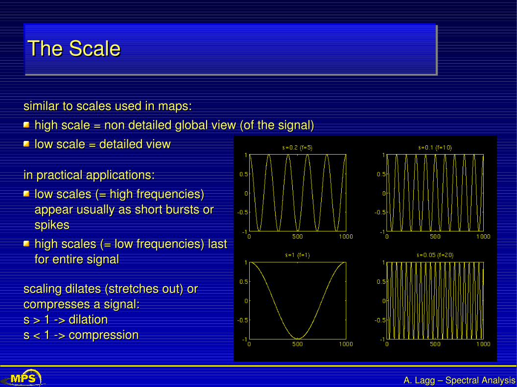
The ScaleThe Scale
similar to scales used in maps:similar to scales used in maps:
high scale = non detailed global view (of the signal)high scale = non detailed global view (of the signal)
low scale = detailed viewlow scale = detailed view
scaling dilates (stretches out) or scaling dilates (stretches out) or compresses a signal:compresses a signal:s > 1 > dilations > 1 > dilations < 1 > compressions < 1 > compression
in practical applications:in practical applications:
low scales (= high frequencies) low scales (= high frequencies) appear usually as short bursts or appear usually as short bursts or spikesspikes
high scales (= low frequencies) last high scales (= low frequencies) last for entire signalfor entire signal

A. Lagg – Spectral AnalysisA. Lagg – Spectral Analysis
Computation of the CWTComputation of the CWT
signal to be analyzed: x(t), mother wavelet: Morlet or Mexican Hatsignal to be analyzed: x(t), mother wavelet: Morlet or Mexican Hat
start with scale s=1 (lowest scale, start with scale s=1 (lowest scale, highest frequency)highest frequency)> most compressed wavelet> most compressed wavelet
shift wavelet in time from tshift wavelet in time from t00 to t to t11
increase s by small valueincrease s by small value
shift dilated wavelet from tshift dilated wavelet from t00 to t to t11
repeat steps for all scalesrepeat steps for all scales

A. Lagg – Spectral AnalysisA. Lagg – Spectral Analysis
CWT ExampleCWT Example
signal x(t)signal x(t)
axes of CWT: translation and axes of CWT: translation and scale (not time and frequency)scale (not time and frequency)
translation > timetranslation > timescale > 1/frequencyscale > 1/frequency

A. Lagg – Spectral AnalysisA. Lagg – Spectral Analysis
Time and Frequency ResolutionTime and Frequency Resolution
every box corresponds to a value of the wavelet every box corresponds to a value of the wavelet transform in the time frequency planetransform in the time frequency plane
all boxes have constant areaall boxes have constant area Δ Δf f ΔΔt = const.t = const.
low frequencies: high resolution low frequencies: high resolution in f, low time resolutionin f, low time resolution
high frequencies: good time high frequencies: good time resolutionresolution
STFT: time and frequency STFT: time and frequency resolution is constant (all boxes resolution is constant (all boxes are the same)are the same)

A. Lagg – Spectral AnalysisA. Lagg – Spectral Analysis
Wavelets: Mathematical ApproachWavelets: Mathematical Approach
CWT x =x
, s =1
∣s∣∫t
x t * t−s dt
Mexican Hat wavelet:Mexican Hat wavelet:
t =1
s3 e−t2
22 t2
2 −1Morlet wavelet:Morlet wavelet:
t = ei a t e−
t2
2
WLtransform:WLtransform:
x t =1c
2 ∫s∫
x , s
1s2 t−
s d dsinverse WLtransform:inverse WLtransform:
c={2∫−∞
∞ ∣∣2
∣∣d }
1/2
∞ with ⇔FT
t admissibility admissibility condition:condition:
A. Lagg – Spectral AnalysisA. Lagg – Spectral Analysis
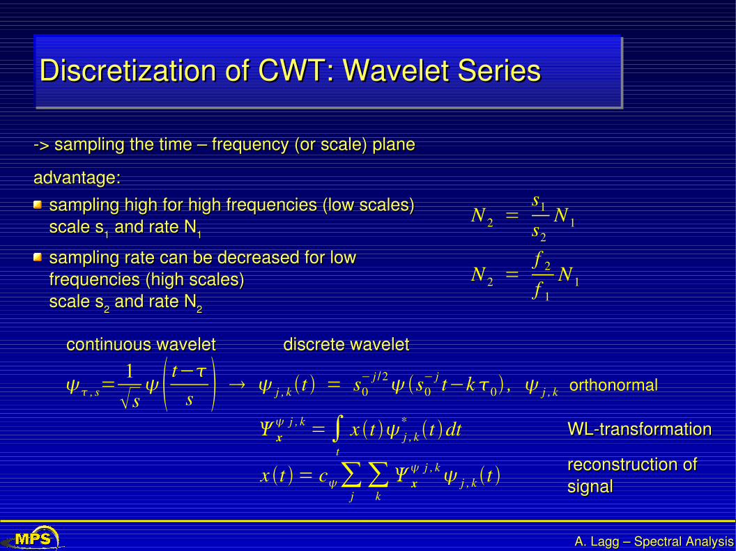
Discretization of CWT: Wavelet SeriesDiscretization of CWT: Wavelet Series
> sampling the time – frequency (or scale) plane> sampling the time – frequency (or scale) plane
advantage:advantage:
sampling high for high frequencies (low scales)sampling high for high frequencies (low scales)scale sscale s11 and rate N and rate N11
sampling rate can be decreased for low sampling rate can be decreased for low frequencies (high scales)frequencies (high scales)scale sscale s22 and rate N and rate N22
N 2 =s1
s2
N 1
N 2 =f 2
f 1
N 1
discrete waveletdiscrete wavelet
, s=1
s t−
s j , k t = s0− j /2s0
− j t−k 0 , j , k orthonormal
continuous waveletcontinuous wavelet
x j , k =∫
t
x t j , k* t dt
x t = c∑j∑
k
x j , k j , k t
WLtransformationWLtransformation
reconstruction of reconstruction of signalsignal

A. Lagg – Spectral AnalysisA. Lagg – Spectral Analysis
Discrete Wavelet TransformDiscrete Wavelet Transform
discretized continuous wavelet transform is only a sampled version of the CWTdiscretized continuous wavelet transform is only a sampled version of the CWT
The discrete wavelet transform (DWT) has significant advantages for The discrete wavelet transform (DWT) has significant advantages for implementation in computers.implementation in computers.
(DWT)(DWT)
excellent tutorial:excellent tutorial:http://users.rowan.edu/~polikar/WAVELETS/WTtutorial.htmlhttp://users.rowan.edu/~polikar/WAVELETS/WTtutorial.html
IDLWavelet Tools:IDLWavelet Tools:IDL> wv_appletIDL> wv_applet
Wavelet expert at MPS:Wavelet expert at MPS:Rajat ThomasRajat Thomas
A. Lagg – Spectral AnalysisA. Lagg – Spectral Analysis
end of Waveletsend of Wavelets

A. Lagg – Spectral AnalysisA. Lagg – Spectral Analysis
ExercisesExercises
Part I: Fourier AnalysisPart I: Fourier Analysis(Andreas Lagg)(Andreas Lagg)
Part II: WaveletsPart II: Wavelets(Rajat Thomas)(Rajat Thomas)
Instructions:Instructions:
http://www.linmpi.mpg.de/~lagghttp://www.linmpi.mpg.de/~lagg
Seminar roomSeminar roomTime: 15:00Time: 15:00
A. Lagg – Spectral AnalysisA. Lagg – Spectral Analysis
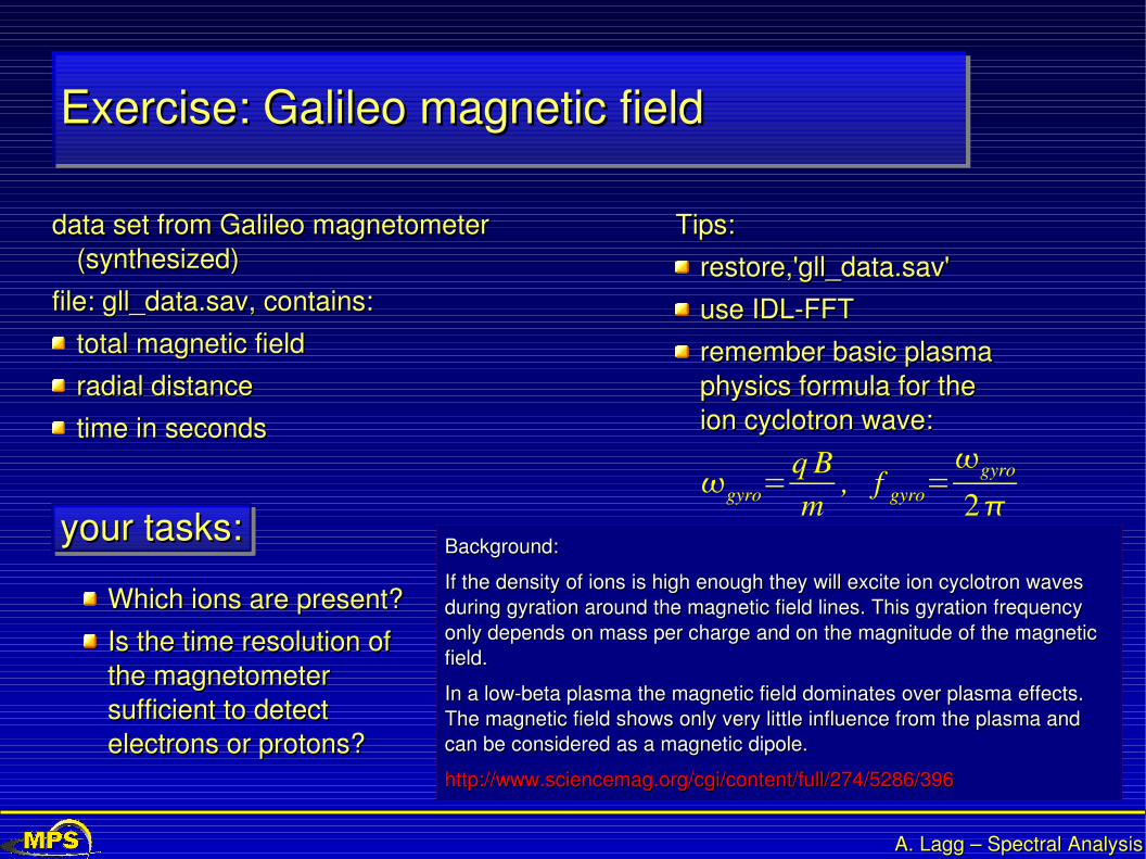
Exercise: Galileo magnetic fieldExercise: Galileo magnetic field
data set from Galileo magnetometer data set from Galileo magnetometer (synthesized)(synthesized)
file: gll_data.sav, contains:file: gll_data.sav, contains:
total magnetic fieldtotal magnetic field
radial distanceradial distance
time in secondstime in seconds
Tips:Tips:
restore,'gll_data.sav'restore,'gll_data.sav'
use IDLFFTuse IDLFFT
remember basic plasma remember basic plasma physics formula for the physics formula for the ion cyclotron wave:ion cyclotron wave:
gyro=q Bm
, f gyro=gyro
2your tasks:your tasks:
Which ions are present?Which ions are present?
Is the time resolution of Is the time resolution of the magnetometer the magnetometer sufficient to detect sufficient to detect electrons or protons?electrons or protons?
Background:Background:
If the density of ions is high enough they will excite ion cyclotron waves If the density of ions is high enough they will excite ion cyclotron waves during gyration around the magnetic field lines. This gyration frequency during gyration around the magnetic field lines. This gyration frequency only depends on mass per charge and on the magnitude of the magnetic only depends on mass per charge and on the magnitude of the magnetic field.field.
In a lowbeta plasma the magnetic field dominates over plasma effects. In a lowbeta plasma the magnetic field dominates over plasma effects. The magnetic field shows only very little influence from the plasma and The magnetic field shows only very little influence from the plasma and can be considered as a magnetic dipole.can be considered as a magnetic dipole.
http://www.sciencemag.org/cgi/content/full/274/5286/396http://www.sciencemag.org/cgi/content/full/274/5286/396

A. Lagg – Spectral AnalysisA. Lagg – Spectral Analysis
LiteratureLiterature
Random Data: Analysis and Measurement ProceduresRandom Data: Analysis and Measurement ProceduresBendat and Piersol, Wiley Interscience, 1971Bendat and Piersol, Wiley Interscience, 1971
The Analysis of Time Series: An IntroductionThe Analysis of Time Series: An IntroductionChris Chatfield, Chapman and Hall / CRC, 2004Chris Chatfield, Chapman and Hall / CRC, 2004
Time Series Analysis and Its ApplicationsTime Series Analysis and Its ApplicationsShumway and Stoffer, Springer, 2000Shumway and Stoffer, Springer, 2000
The Wavelet TutorialThe Wavelet TutorialRobi Polikar, 2001Robi Polikar, 2001http://users.rowan.edu/~polikar/WAVELETS/WTtutorial.htmlhttp://users.rowan.edu/~polikar/WAVELETS/WTtutorial.html
Numerical Recipies in CNumerical Recipies in CCambridge University Press, 19881992Cambridge University Press, 19881992http://www.nr.com/http://www.nr.com/