Special Relativistic (Flight-)Simulator

Anton Tsoulos† and Wolfgang Knopki∗

Abstract—With special relativistic visualisation it is possible to experience and simulate relativistic effects which occur whentraveling close to the speed of light. These effects are geometric distortions, like length contraction, as well as optical effects forexample the Doppler and the searchlight effect. There are various approaches to implement these physical effects; image-basedrendering, polygon rendering or ray tracing to name but a few. In this paper we take a closer look at image-based renderingaswell as polygon rendering with the aim to, create an other method, called advanced polygon rendering. Advanced polygonrendering is a further development of polygon rendering to provide better results compared to regular polygon rendering. Ourimplementation uses an open source 3D engine to load scenes with little effort, as well as GPU shader programming with modernOpenGL to achieve best performance.

Index Terms—Visualisation in Physical Sciences and Engineering, special relativity, advanced polygon rendering, image-basedrendering

1 INTRODUCTION

Since its publication in 1905 Einstein’s theory of relativity has beenin the center of modern physics. But unlike traditional Newtonianphysics, its effects are hard to observe and experiments aiming atits observation are becoming increasingly big and costly. Computa-tional simulation of relativistic effects has thus become a vital partin modern physics.

These effects in particular compose of the Doppler effect, beingthe shift of spectrum of the light emitted by a visible object. Asthe speed of the observer changes, so does the wavelength of theobserved light which may cause a shift of spectrum from the formerlyinvisible infrared or ultraviolet part into the visible spectrum. Forexample heat radiation emitted by objects turns now visible.

(a) (b)

Figure 1: The aberration effect explained: Image (a) shows theobserver at rest: Light reaches him equally distributed from all sides.Image (b) shows the observer in motion to the right, light previouslyreaching him from the sides now comes from ahead

Other effects that can be observed are aberration effects such asthe distortion of the surrounding. The light that seemingly reachedthe observer from a certain direction while he is moving at low ve-locities seems to come from other directions (see Figure 1). Objectsthat are behind the observer do now appear sideways or in frontof the observer and the objects in front of the observer seem to besmaller and thus increasingly distant.

2 RELATED WORK

Due to its nature, the observation of relativistic effects relies purelyon computational simulation, since these effects can not be observedunder normal circumstances found on earth as it is technically im-possible to reach velocities even far from the speed of light. As

† Anton Tsoulos ∗Wolfgang Knopkianton.tsoulos@ilw.uni-stuttgart.de wolfgang.knopki@ilw.uni-stuttgart.de

described by Weiskopf [12] and Muller [8], first visualisation at-tempts date as far back as 1924. Visualisation of special relativisticeffects by means of computation, however, are a relatively new fieldof study: In 1989 Taylor [11] developed tools for educational pur-poses. Fully interactive visualisations of relativistic effects are evenmore recent: In 2005, Kraus and Borchers offered a relativistic bikeride through the ancient center of Tubingen (see [5]), and in 2007,Savage et al. [10] developed a first person simulation of relativisticeffects in an image-based approach.

Most recently, there have been further publications in the fieldof special relativistic visualisation: In 2010, Muller et al. [8] andWeiskopf [12] used polygon rendering and local ray-tracing tech-niques to visualize relativistic effects. Unlike the formerly widelyused image-based methods, these do not have the issue of increas-ingly poor resolutions with high velocities and therefore high ratesof distortion (details are discussed in Section 3.1.1)

3 OUR APPROACH

The goal attained by this project was to get a discussion base forvisualisation of relativistic effects and hereby compare the primitiveimage based approach with the approach of ”advanced” polygonrendering. Advancing in polygon-rendering is the amelioration of”simple” polygon rendering by creating new vertices depending onthe curvature of the scene elements.

A further goal was to adapt an existing game engine to our needsto provide possible future support for relativistic game development.

Concerning the engine used, we decided on Irrlicht [2], a freeengine whose most attractive feature was the ability to easily load avariety of scene formats including Quake 3 levels (.bsp) or OGREmeshes (.mesh). As graphics API OpenGL was used for the sakeof OS-interoperability, although Irrlicht also offers the usage ofDirectX.

3.1 Image-Based Part

To complete the task of special relativistic simulation in animage-based approach we use a shortened version of the classicalgraphics pipeline. The scene is at first rendered six times by sixcameras that are orthogonal. These cameras have each a field ofview of 90◦ × 90◦. The images obtained through these camerasare then put together to one cubemap texture that is projected on afull screen quad implemented as a screen-sized rectangle. Duringthis projection, relativistic effects are added by means of fragmentshading. To do so, we reverted to the formula of aberration obtainedthrough the Lorentz-transformation as described by Muller et al. [9]

Let the velocity of light be denoted as c.

1

Let S’ be a system in motion with velocity v with respect to S

β =vc,

γ =1√

1−β 2,

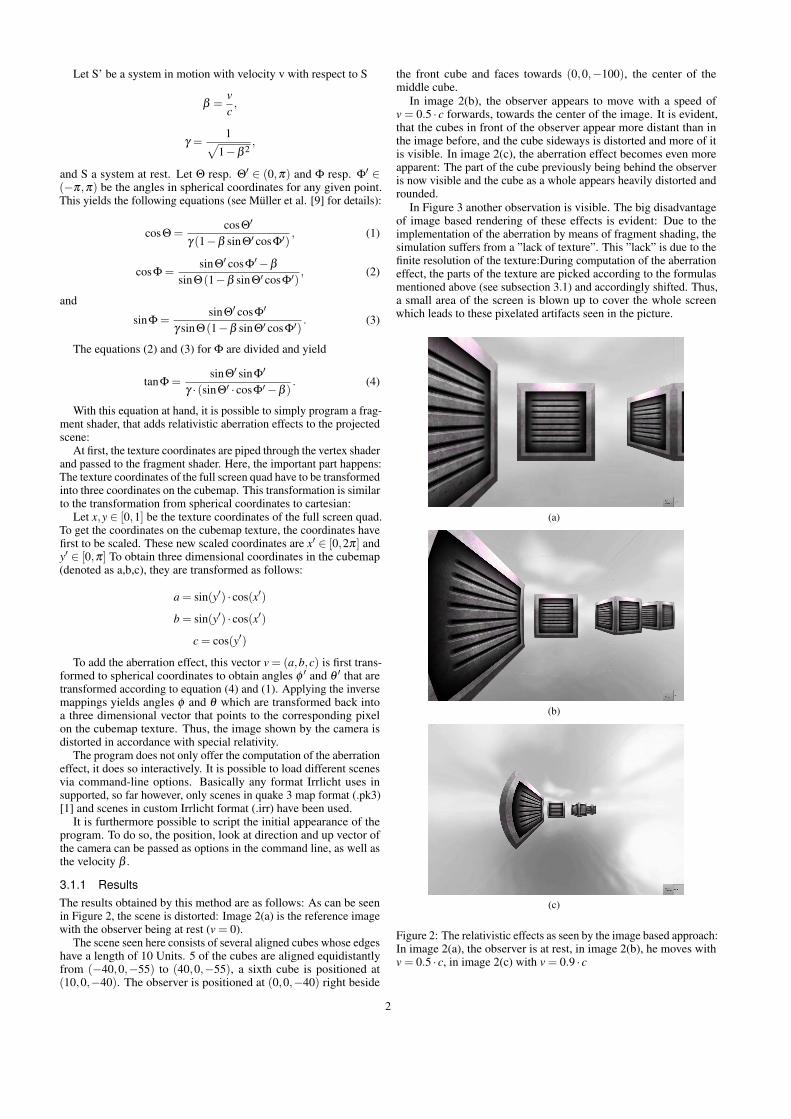
and S a system at rest. Let Θ resp. Θ′ ∈ (0,π) and Φ resp. Φ′ ∈(−π,π) be the angles in spherical coordinates for any given point.This yields the following equations (see Muller et al. [9] for details):

cosΘ =cosΘ′

γ (1−β sinΘ′ cosΦ′), (1)

cosΦ =sinΘ′ cosΦ′−β

sinΘ(1−β sinΘ′ cosΦ′), (2)

and

sinΦ =sinΘ′ cosΦ′

γ sinΘ(1−β sinΘ′ cosΦ′). (3)

The equations (2) and (3) for Φ are divided and yield

tanΦ =sinΘ′ sinΦ′

γ · (sinΘ′ · cosΦ′−β ). (4)

With this equation at hand, it is possible to simply program a frag-ment shader, that adds relativistic aberration effects to the projectedscene:

At first, the texture coordinates are piped through the vertex shaderand passed to the fragment shader. Here, the important part happens:The texture coordinates of the full screen quad have to be transformedinto three coordinates on the cubemap. This transformation is similarto the transformation from spherical coordinates to cartesian:

Let x,y ∈ [0,1] be the texture coordinates of the full screen quad.To get the coordinates on the cubemap texture, the coordinates havefirst to be scaled. These new scaled coordinates are x′ ∈ [0,2π] andy′ ∈ [0,π] To obtain three dimensional coordinates in the cubemap(denoted as a,b,c), they are transformed as follows:

a = sin(y′) · cos(x′)

b = sin(y′) · cos(x′)

c = cos(y′)

To add the aberration effect, this vector v = (a,b,c) is first trans-formed to spherical coordinates to obtain angles φ ′ and θ ′ that aretransformed according to equation (4) and (1). Applying the inversemappings yields angles φ and θ which are transformed back intoa three dimensional vector that points to the corresponding pixelon the cubemap texture. Thus, the image shown by the camera isdistorted in accordance with special relativity.

The program does not only offer the computation of the aberrationeffect, it does so interactively. It is possible to load different scenesvia command-line options. Basically any format Irrlicht uses insupported, so far however, only scenes in quake 3 map format (.pk3)[1] and scenes in custom Irrlicht format (.irr) have been used.

It is furthermore possible to script the initial appearance of theprogram. To do so, the position, look at direction and up vector ofthe camera can be passed as options in the command line, as well asthe velocity β .

3.1.1 ResultsThe results obtained by this method are as follows: As can be seenin Figure 2, the scene is distorted: Image 2(a) is the reference imagewith the observer being at rest (v = 0).

The scene seen here consists of several aligned cubes whose edgeshave a length of 10 Units. 5 of the cubes are aligned equidistantlyfrom (−40,0,−55) to (40,0,−55), a sixth cube is positioned at(10,0,−40). The observer is positioned at (0,0,−40) right beside

the front cube and faces towards (0,0,−100), the center of themiddle cube.

In image 2(b), the observer appears to move with a speed ofv = 0.5 · c forwards, towards the center of the image. It is evident,that the cubes in front of the observer appear more distant than inthe image before, and the cube sideways is distorted and more of itis visible. In image 2(c), the aberration effect becomes even moreapparent: The part of the cube previously being behind the observeris now visible and the cube as a whole appears heavily distorted androunded.

In Figure 3 another observation is visible. The big disadvantageof image based rendering of these effects is evident: Due to theimplementation of the aberration by means of fragment shading, thesimulation suffers from a ”lack of texture”. This ”lack” is due to thefinite resolution of the texture:During computation of the aberrationeffect, the parts of the texture are picked according to the formulasmentioned above (see subsection 3.1) and accordingly shifted. Thus,a small area of the screen is blown up to cover the whole screenwhich leads to these pixelated artifacts seen in the picture.

(a)

(b)

(c)

Figure 2: The relativistic effects as seen by the image based approach:In image 2(a), the observer is at rest, in image 2(b), he moves withv = 0.5 · c, in image 2(c) with v = 0.9 · c

2

(a)

(b)

Figure 3: ”Lack of texture” caused by limited resolution of thetexture: Movement backwards with v = 0.9 · c in image 3(b), nomovement in image 3(a)

3.2 Advanced Polygon Rendering

The main idea of polygon rendering is the transformation of (all)points or objects from their 3D reference frame into the 3D refer-ence frame of an observer. The result of this transformation is aso-called photo-object which is a virtual object which shows theposition where the light rays must been emitted to reach the observersimultaneously. However we develop Advanced Polygon Render-ing (APR) in order to show and improve the rendered effects ofthe special relativity and the quality of the image and consequentlythe photo-objects at high speed. Due to the special relativitiy, inhigh speed, geometrical objects appear distorted, for example an un-bowed rod becomes formed as a hyperbola when it is flying towardsan observer, as seen in Figure 4.

Since we want to know what an observer sees, we have to mindthe time which the light needs to reach the observer from an event,to create a photo-object. However, special relativity views space andtime not as separate features but as a unity, which is called spacetime.A point within the spacetime can be described by a 4-dimensionalvector x = (ct,x,y,z) containing the time and the 3D-coordinates ofthe event. The effect of the unbowed rod which becomes bowed onhigh speed can be then explained by the finite speed of light. Lightrays from both ends of the rod must be emitted earlier than from thecenter in order to reach the observer simultaneously. Since the rod isstill approaching, the time which the light needs to reach the observerdescends, points closer to the center of the rod are emitting lightrays much later than from the edges. Considering both, time andspace, all the single emission points taken together form a hyperbola.Increasing β would even lead to a stronger curved hyperbola, up toa sharp edge.

Unfortunately because of these effects, an image from a meshwith few vertices, created with regular polygon rendering does notshow the reality like it is supposed to be. Instead just distorted ob-

(a) (b) (c)

Figure 4: Example of a rod under the influences of special relativisticeffects; (a) shows the rod at rest with β = 0. In (b) the rod movesinto direction of the observer with β = 0.9 with a kind of ”zooming”-effect in the center of the rod. (c) shows the same rod as (b) from asideview, whereby the distortion of the rod in form of a hyperbola isclearly visible. The observer is thereby in front and in the center ofthe rod.

jects without curvatures or with strong edged curvatures can be seen,due to the non-linearity of the transformation into the photo-objectand the minor tessellation of the object itself. By using advancedpolygon rendering we try to minimize the effect to create graphicsand scenes with higher quality of rendered objects. The possibilityto use advanced polygon rendering came first in the last couple ofyears with the development of modern graphic cards and the intro-duction of programmable graphics pipeline which can be controlledby shaders. Under these conditions, we were using modern OpenGL(OpenGL 4.0 and greater) which gave us the important opportunityto use tessellation shaders which we greatly used. With tessellationshader we can divide huge objects, respectively the triangles or otherprimitives they are assembled of, into smaller ones to increase thequality of the picture and the granularity of an object. In our examplethe primitives of the rod becomes divided into smaller primitiveswhich can be placed to approximate a curve.

The tessellation shaders are however not the only way for geome-try subdivision. The geometry shader can be used as well, but even ifit is also capable of this kind of work, the usage of tessellation shaderis preferred since the exclusive use of the geometry shader carriesproblems with it. The first problem is that the number of primitives,generated by one instance of the geometry shader varies becausesome objects require a higher tessellation level than other whichcould lead to problems with the synchronization of data emissionsand the order in what output primitives will take place in the outputbuffer. Another problem is that the geometry subdivision withina single shader is done iteratively, which is quite a waste in caseof a highly parallelized processors like a GPU, which results in areasonable amount of delay. Because of these reasons, the preferredway to create a geometry subdivision are the tessellation shaders.These preconditions allow us to use the graphic pipeline as follows:

• The vertex shader is only passing the position of the verticesmultiplied by the world-matrix, to transform the vertices with-ion the 3D-world and not in the 2D-image and the texturecoordinates to appropriate map the textures later, to the nextshader.

• The tessellation control shader determines the tessellation lev-els and passes the vertices to the evaluation shader.

• The tessellation evaluation shader is evaluating the points andtransforms the additional vertices accordingly.

3

• The fragment shader itself does nothing more than to samplethe textures and writing the color.

3.2.1 Implementation of APRWe assume at least three different reference frames; The referenceframe of the observer and one or more reference reference frames inwhich our objects are, as shown in Figure 5. These reference framesare in a global frame which contain all other. To describe an event,which occurred in its reference frame, in the reference frame of theobserver we need the Poincare-transformation. Thus it is neededto calculate the required Lorentz-matrices, see equitation (5) andtheir inverse for each frame to Poincare-transform all vertices ofthe objects, from their reference frame to the reference frame of theobserver, in order to find the time where the object must emit a lightray to be visible for the observer.

Figure 5: Scheme of the different frames within the world

While it is not necessary, in our approach the observer is notmoving and thus the speed (and beta) is zero, however the objectscan move freely. So we need to calculate a Lorentz-matrix Λβ andits inverse Λβ for the static observer aswell as the correspondingmatrices for each moving reference frame of the objects.

Λβ =

γ −γ

vxc −γ

vyc −γ

vzc

−γvxc

−γvyc 13 +

γ2

1+γ· v⊕v

c2

−γvzc

(5)

The Poincare-transformation transforms the position of a pointfrom its reference frame to an other reference frame. We use usethis transformation to transform the observer from its rest frame S’into the global frame S (6) and then again to transform the new pointfrom the global frame into the reference frame of the object S” (7).

xobs = Λβ1x′obs +a1 (6)

x′′obs = Λβ2(xobs−a2) (7)

While in our approach we assume that a1 and a2 for the relativeshift of the systems are null vectors (meaning the systems are over-laid), it is not necessary. Furthermore we assume that the coordinatesystems are axis-aligned.

Doing so, a Minkowski-diagram can be used to depict the positionof the observer and the position of the point within the spacetime andrelative to each other. Minkowski-diagrams have the advantage that

Figure 6: Schematic intersection of the worldline of the point withthe backward light cone of the observer. They intersect at positionx′′i at time t ′′i , which is the time we want to know

they often show a picturesque description of movement of an objectin spacetime. They illustrate the mathematical properties of spaceand time in the special relativity with the time as y-axis and the spaceas x-axis. Having transformed the observer from its reference frameto the reference frame of the point, it is then possible to calculate thetime t ′′i in which the observer is able to see the point. This can beachieved by calculating the intersection of the worldline of the pointwith the backward light cone of the observer, as seen in Figure 6.Because of the finite speed of light the observer can only see eventshappened in the past, thus it is only necessary to intersect with thebackward cone and to ignore the forward cone. ∆ here returns thelength of the difference of two vectors.

x′′0ob j = t ′′i = x

′′0obs−∆(x

′′ob j,x

′′obs) (8)

Calculating the intersection between the worldline of the point andthe light cone of the observer yields the time where a light raymust be emitted from this point in order to reach the observer atobservation time (8). Having the time in which the observer willsee the point, the point itself is now transformed into the referenceframe of the observer using the same transformations vice versa (9)and (10).

xob j = Λβ2x′′ob j +a2 (9)

x′ob j = Λβ1(xob j−a1) (10)

With the last inverse transformation (10), the position of the pointwhere it will be visible at observation time, was calculated. Thistransformation is needed, since it is necessary to place the objects totheir right place within the tessellation evaluation shader to createthe photo-object. Nevertheless all these Poincare-transformationshave to be repeated if the observation time or the position of theobserver or objects changes.

Until to this point, there are little changes compared to regularpolygon rendering. However it is still unknown which tessellationlevel is needed to see the correct relativistic distortions at high speed.The main and new part, the calculation of the tessellation level hap-pens in the tessellation control shader. Given a triangle as input wetake a pair of vertices and calculate the direction vector #»r = #»v1− #»v2from one vertex to the other. From both vertices a minimal dis-tance δ is taken to create another point into direction to the othervertex, to get a pair of two tuple with points t1 = ( #»v1,

#»v1 + δ · #»r )and t2 = ( #»v2,

#»v2− δ · #»r ). Afterwards all four points will be trans-formed into the rest frame of S’ using the double-staged Poincare

4

transformation, receiving the tuple t ′1 and t ′2 with the transformedpoints. With these two tuples it is now possible to calculate two tan-gents for which we further calculate the angle between them (Figure7). The angle between both tangents is an indicator how strong the

Figure 7: Schema how to get the angle α from a tuple of vertices of atriangle. With a distance δ two other points into the direction of theother vertex are taken, getting two tuples. Poincare-transforming all4 points results in the tuples t ′1 = (v′1,v

′11) and t ′2 = (v′2,v

′22). With

them, two tangents can be calculated, and intersecting them yieldsthe angle α .

transformation is, for example how much a line bends depending onvelocity. A small angle means stronger bending, whereas a big anglemeans that the special relativistic effects are not that strong. Withhelp of the angle it is possible to compute the level of tessellation.However it is important to consider that the effects of relativity arenot linear but increase exponentially with higher speed, thus theangle decreases faster the faster the observer moves. These stepsshall be repeated for all possible combinations of pairs, getting thetessellation level for each side of the triangle. Not in possession of agood fomula we used an approximation which gave us acceptableresults, by choosing the appropriate tesselation levels when the angleis within an specific range.

• 180 - 171 degree: tesselation level = 1

• 171 - 163 degree: tesselation level = 2

• 163 - 147 degree: tesselation level = 4

• 147 - 118 degree: tesselation level = 8

• 118 - 96 degree: tesselation level = 16

• 32 otherwise

Anyway this is just an approximation used in our approach, obviouslya better solution is to develop a calculation specification to get thetessellation level directly and by not using ranges.

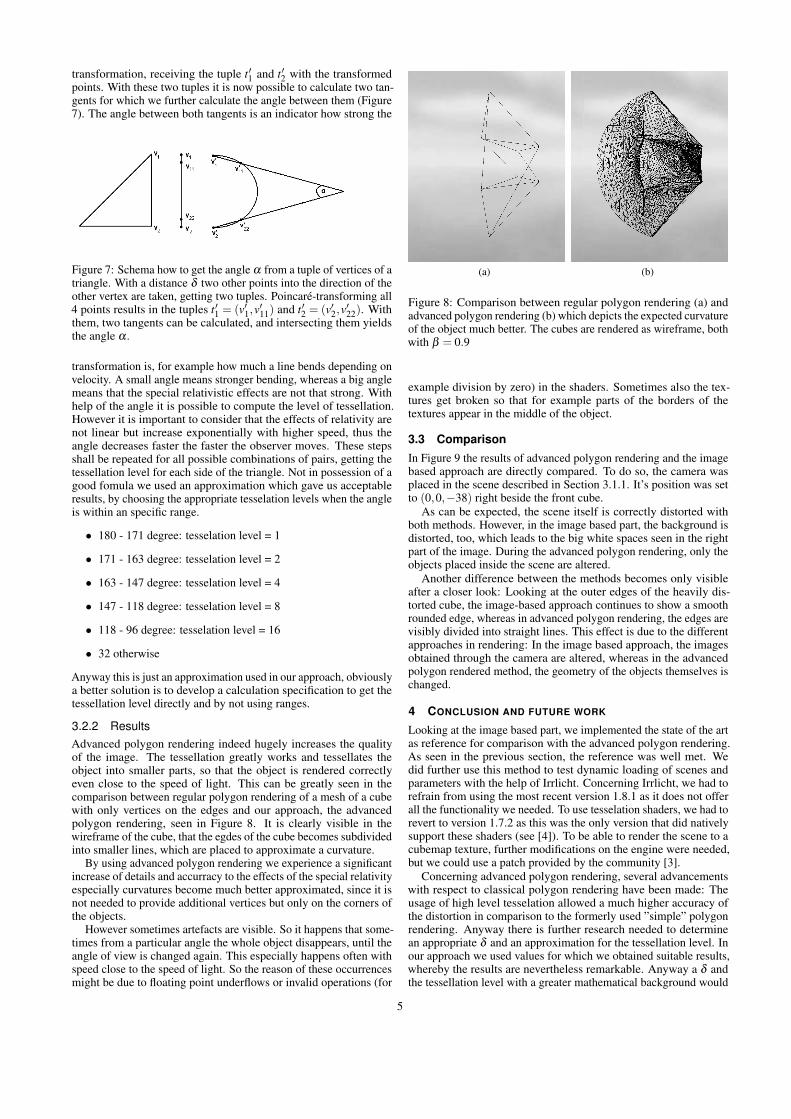
3.2.2 ResultsAdvanced polygon rendering indeed hugely increases the qualityof the image. The tessellation greatly works and tessellates theobject into smaller parts, so that the object is rendered correctlyeven close to the speed of light. This can be greatly seen in thecomparison between regular polygon rendering of a mesh of a cubewith only vertices on the edges and our approach, the advancedpolygon rendering, seen in Figure 8. It is clearly visible in thewireframe of the cube, that the egdes of the cube becomes subdividedinto smaller lines, which are placed to approximate a curvature.

By using advanced polygon rendering we experience a significantincrease of details and accurracy to the effects of the special relativityespecially curvatures become much better approximated, since it isnot needed to provide additional vertices but only on the corners ofthe objects.

However sometimes artefacts are visible. So it happens that some-times from a particular angle the whole object disappears, until theangle of view is changed again. This especially happens often withspeed close to the speed of light. So the reason of these occurrencesmight be due to floating point underflows or invalid operations (for

(a) (b)

Figure 8: Comparison between regular polygon rendering (a) andadvanced polygon rendering (b) which depicts the expected curvatureof the object much better. The cubes are rendered as wireframe, bothwith β = 0.9

example division by zero) in the shaders. Sometimes also the tex-tures get broken so that for example parts of the borders of thetextures appear in the middle of the object.

3.3 ComparisonIn Figure 9 the results of advanced polygon rendering and the imagebased approach are directly compared. To do so, the camera wasplaced in the scene described in Section 3.1.1. It’s position was setto (0,0,−38) right beside the front cube.

As can be expected, the scene itself is correctly distorted withboth methods. However, in the image based part, the background isdistorted, too, which leads to the big white spaces seen in the rightpart of the image. During the advanced polygon rendering, only theobjects placed inside the scene are altered.

Another difference between the methods becomes only visibleafter a closer look: Looking at the outer edges of the heavily dis-torted cube, the image-based approach continues to show a smoothrounded edge, whereas in advanced polygon rendering, the edges arevisibly divided into straight lines. This effect is due to the differentapproaches in rendering: In the image based approach, the imagesobtained through the camera are altered, whereas in the advancedpolygon rendered method, the geometry of the objects themselves ischanged.

4 CONCLUSION AND FUTURE WORK

Looking at the image based part, we implemented the state of the artas reference for comparison with the advanced polygon rendering.As seen in the previous section, the reference was well met. Wedid further use this method to test dynamic loading of scenes andparameters with the help of Irrlicht. Concerning Irrlicht, we had torefrain from using the most recent version 1.8.1 as it does not offerall the functionality we needed. To use tesselation shaders, we had torevert to version 1.7.2 as this was the only version that did nativelysupport these shaders (see [4]). To be able to render the scene to acubemap texture, further modifications on the engine were needed,but we could use a patch provided by the community [3].

Concerning advanced polygon rendering, several advancementswith respect to classical polygon rendering have been made: Theusage of high level tesselation allowed a much higher accuracy ofthe distortion in comparison to the formerly used ”simple” polygonrendering. Anyway there is further research needed to determinean appropriate δ and an approximation for the tessellation level. Inour approach we used values for which we obtained suitable results,whereby the results are nevertheless remarkable. Anyway a δ andthe tessellation level with a greater mathematical background would

5

(a) β = 0.0 (b) β = 0.0

(c) β = 0.9 (d) β = 0.9

(e) detailed view of the outer edge (f) detailed view of the outer edge

Figure 9: Direct comparison between the two methods: AdvancedPolygon Rendering on the left, image based on the right.

be much better for professional usage and probably increase thequality even more. It is also necessary to find the reason why theartefacts appear and the objects disappear sometimes and how this isavoidable. We also set the inner tesselation level to the maximumof the three calculated outer tessellation levels, here an other waymight be more suitable. Furthermore it would be interesting todetermine a maximum tessellation level which do not let collapse theperformance of the image rendering unnecessarily. Since we useda maximum tessellation level of 32, even if tessellation levels up to64 and even higher are possible, and worked with uncomplicatedscenes and meshes, a comparison of the costs is difficult and hasnot been done yet. Therefore there is great potential to improvethis method and obtain a better solution. By using greater andmore complicated scenes a kind of benchmarking to find out whichmethod results in better performance with acceptable quality andunder what circumstances is needed and should be done, as theuse of tessellation shader for geometry subdivision involves somemore overhead compared to the image-based approach or the simpleversion of polygon rendering.

Another vital part in researching special relativistic simulation isthe approach of local ray tracing. Implementing this third methodand comparing these three methods with each other is part of futurework.

ACKNOWLEDGMENTS

The authors like to thank Dr. Thomas Muller, Dr. Sebastian Boblestand Dipl.-Inf Alexandros Panagiotidis for their support and help. Wewould like to further thank our former co-author Melanie Knupferfor her participation.

REFERENCES

[1] ”inner sanctum” katdm3 custom quake 3 level : Katsbits maps.http://www.katsbits.com/download/maps/quake-3/inner-sanctum.php.

[2] Irrlicht engine - a free open source 3d engine. http://irrlicht.sourceforge.net/.

[3] Irrlicht with cubemap support. http://irrlicht.sourceforge.net/forum/viewtopic.php?t=44884.

[4] Opengl tesselation. http://irrlicht.sourceforge.net/forum/viewtopic.php?f=2&t=44195.

[5] U. Kraus and M. Borchers. Visualisierung relativistischer Effekte: FastLichtschnell durch die Stadt. Physik in unserer Zeit, 2(2):64–69, 2005.

[6] T. Muller and S. Boblest. Visual appearance of wireframe objects inspecial relativity. European Journal of Physics, 35:065025, 2014.

[7] T. Muller and D. Weiskopf. Special-relativistic visualization. Comput-ing in Science & Engineering, 13(4):85–93, 2011.

[8] T. Muller, S. Grottel, and D. Weiskopf. Special relativistic visualizationby local ray tracing. Visualization and Computer Graphics, IEEETransactions on, 16(6):1243–1250, 2010.

[9] T. Muller, A. King, and D. Adis. A trip to the end of the universeand the twin “paradox”. American Journal of Physics, 76(4):360–373,2008.

[10] C. M. Savage, A. Searle, and L. McCalman. Real time relativity:Exploratory learning of special relativity. American Journal of Physics,75(9):791–798, 2007.

[11] E. Taylor. Space-time software: Computer graphics utilities in specialrelativity. American Journal of Physics, 57:508–514, 1989.

[12] D. Weiskopf. A Survey of Visualization Methods for Special Relativ-ity. In H. Hagen, editor, Scientific Visualization: Advanced Concepts,volume 1 of Dagstuhl Follow-Ups, pages 289–302. Schloss Dagstuhl–Leibniz-Zentrum fuer Informatik, Dagstuhl, Germany, 2010.

6