Speaker: Mark Hegberg - NEBB Mark Hegberg Application of the Hydronic System Curve: Simple but...
67
Transcript of Speaker: Mark Hegberg - NEBB Mark Hegberg Application of the Hydronic System Curve: Simple but...

Speaker: Mark Hegberg
Application of the Hydronic System
Curve: Simple but Powerful Tool for
Achieving System Performance

The ASHRAE Systems Handbook Describes
1
2
2
1
2
2
h
h
Q
Q
Head Known
Head New
Flow Known
Flow New
• Many answers to balancing issues can be given "depth" by using the System Curve concept as a simple analysis tool of the hydronic system
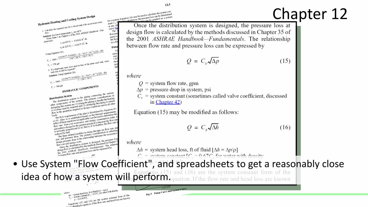
Chapter 12
• Use System "Flow Coefficient", and spreadsheets to get a reasonably close idea of how a system will perform.
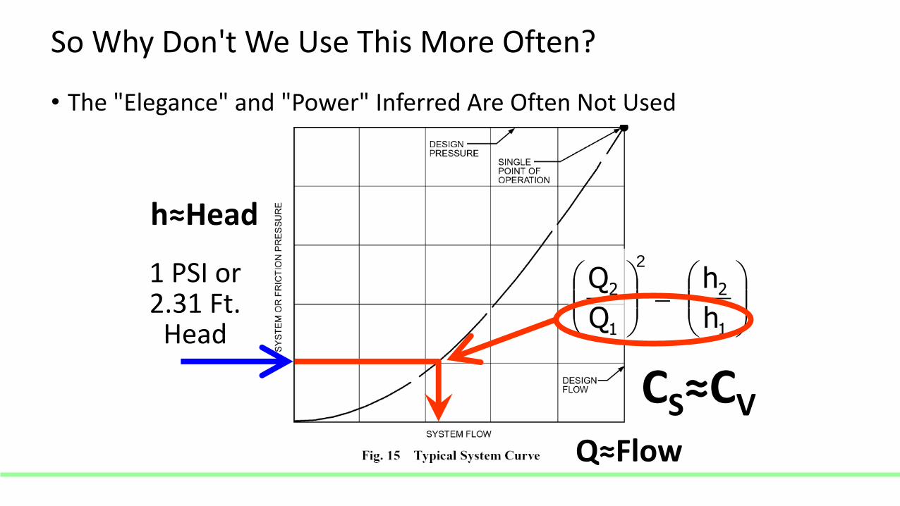
So Why Don't We Use This More Often?
• The "Elegance" and "Power" Inferred Are Often Not Used
1 PSI or 2.31 Ft.
Head
h≈Head
Q≈Flow
1
2
1
2
h
h
Q
Q2
CS≈CV
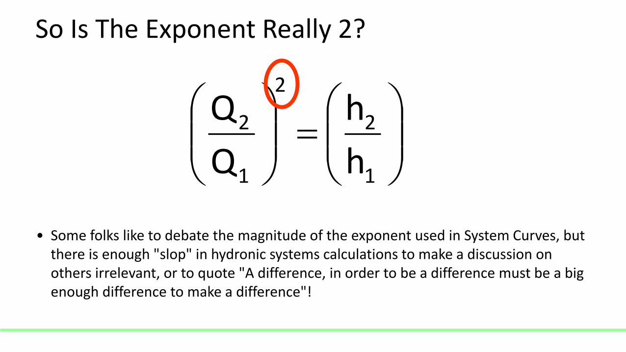
So Is The Exponent Really 2?
1
2
2
1
2
h
h
Q
Q
• Some folks like to debate the magnitude of the exponent used in System Curves, but there is enough "slop" in hydronic systems calculations to make a discussion on others irrelevant, or to quote "A difference, in order to be a difference must be a big enough difference to make a difference"!
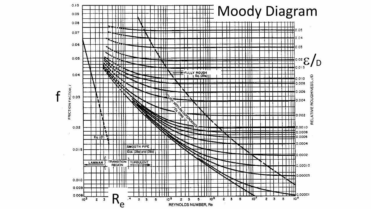
Moody Diagram
f
Re
e/ D

6” Pipe
• In normal design range; close enough
• Fitting losses are very inaccurate
April 4, 2014 2014 NEBB National Conference Tech Session; Making Systyem Curves Work For You 8
2 FPS 10 FPS
> 4
40
0 H
OU
RS
20
00
> <
44
00
HO
UR
S
< 2
00
0 H
OU
RS
X2
X1.89
FRIC
TIO
N F
AC
TOR
FRIC
TIO
N L
OSS
PER
10
0 F
T
FLOW RATE GPM
7.6 FPS 12.2 FPS

So why bring the subject up?
• There are two different methods • Darcy-Weisbach (considered more accurate)
• Hazen-Williams
• There are inherent inaccuracies in all fluid calculations • Pumps are not flow meters
• Fitting losses vary by fluid velocity (e.g. “K” factors)
• Certain fittings can have non-logical results, like branch lines of “Tees”
• “Squares” have been the norm for many complimentary calculations
• The method we present is to help apply some fundamental logic and method of calculation… not absolute precision
April 4, 2014 2014 NEBB National Conference Tech Session; Making Systyem Curves Work For You 10
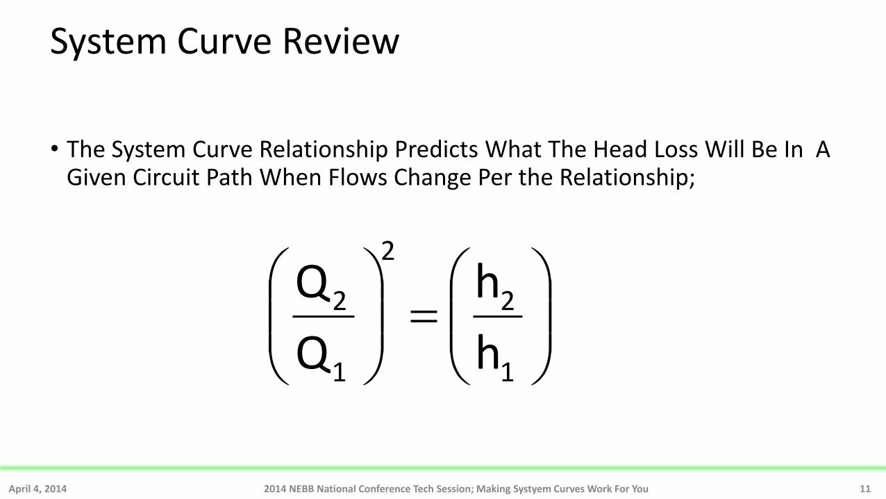
System Curve Review
• The System Curve Relationship Predicts What The Head Loss Will Be In A Given Circuit Path When Flows Change Per the Relationship;
April 4, 2014 2014 NEBB National Conference Tech Session; Making Systyem Curves Work For You 11
1
2
2
1
2
h
h
Q
Q
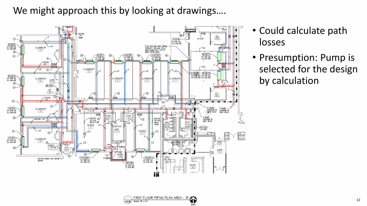
We might approach this by looking at drawings….
• Could calculate path losses
• Presumption: Pump is selected for the design by calculation
12
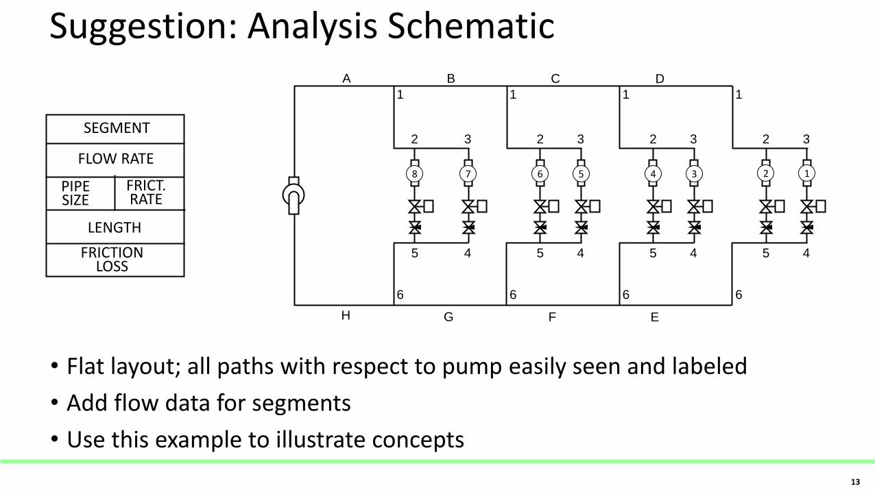
Suggestion: Analysis Schematic
• Flat layout; all paths with respect to pump easily seen and labeled
• Add flow data for segments
• Use this example to illustrate concepts
13
FLOW RATE
PIPE SIZE
FRICT. RATE
LENGTH
FRICTION LOSS
SEGMENT
A B C D
1
2 3
5 4
6
1
2 3
5 4
6
1
2 3
5 4
6
1
2 3
5 4
6
G F E
1 2 3 4 5 6 7 8
H
April 4, 2014 2014 NEBB National Conference Tech Session; Making Systyem Curves Work For You 14
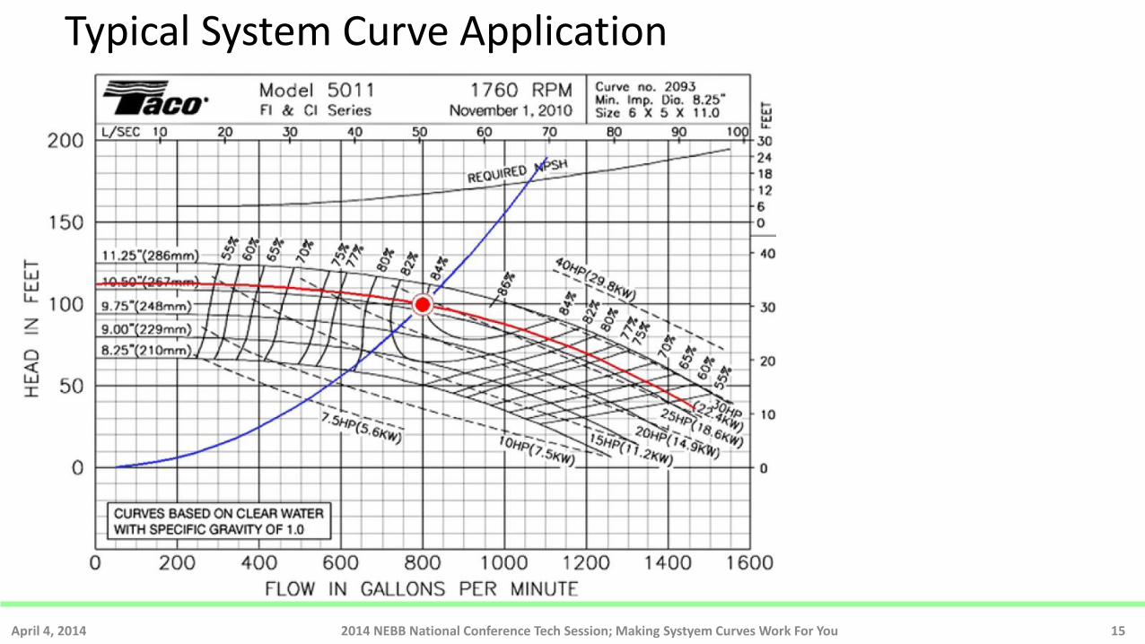
Typical System Curve Application
April 4, 2014 2014 NEBB National Conference Tech Session; Making Systyem Curves Work For You 15
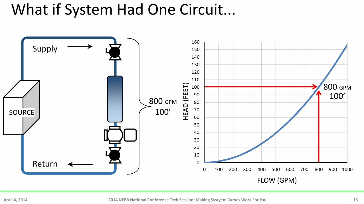
What if System Had One Circuit...
April 4, 2014 2014 NEBB National Conference Tech Session; Making Systyem Curves Work For You 16
800 GPM
100’
Supply
Return
SOURCE
HEA
D (
FEET
) FLOW (GPM)
800 GPM
100’
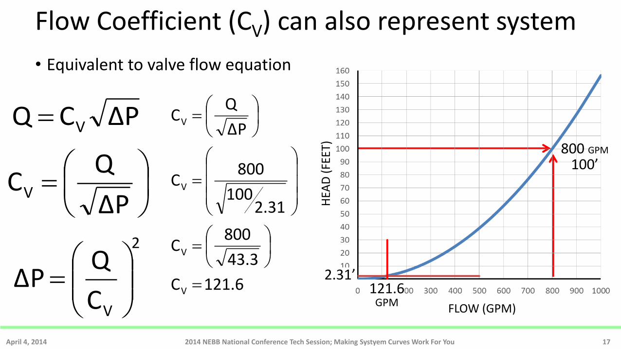
Flow Coefficient (CV) can also represent system
• Equivalent to valve flow equation
April 4, 2014 2014 NEBB National Conference Tech Session; Making Systyem Curves Work For You 17
ΔPCQ V
ΔP
QCV
2
VC
QΔP
121.6 C
43.3
800C
2.31100
800C
ΔP
QC
V
V
V
V
HEA
D (
FEET
)
FLOW (GPM)
800 GPM
100’
2.31’ 121.6
GPM
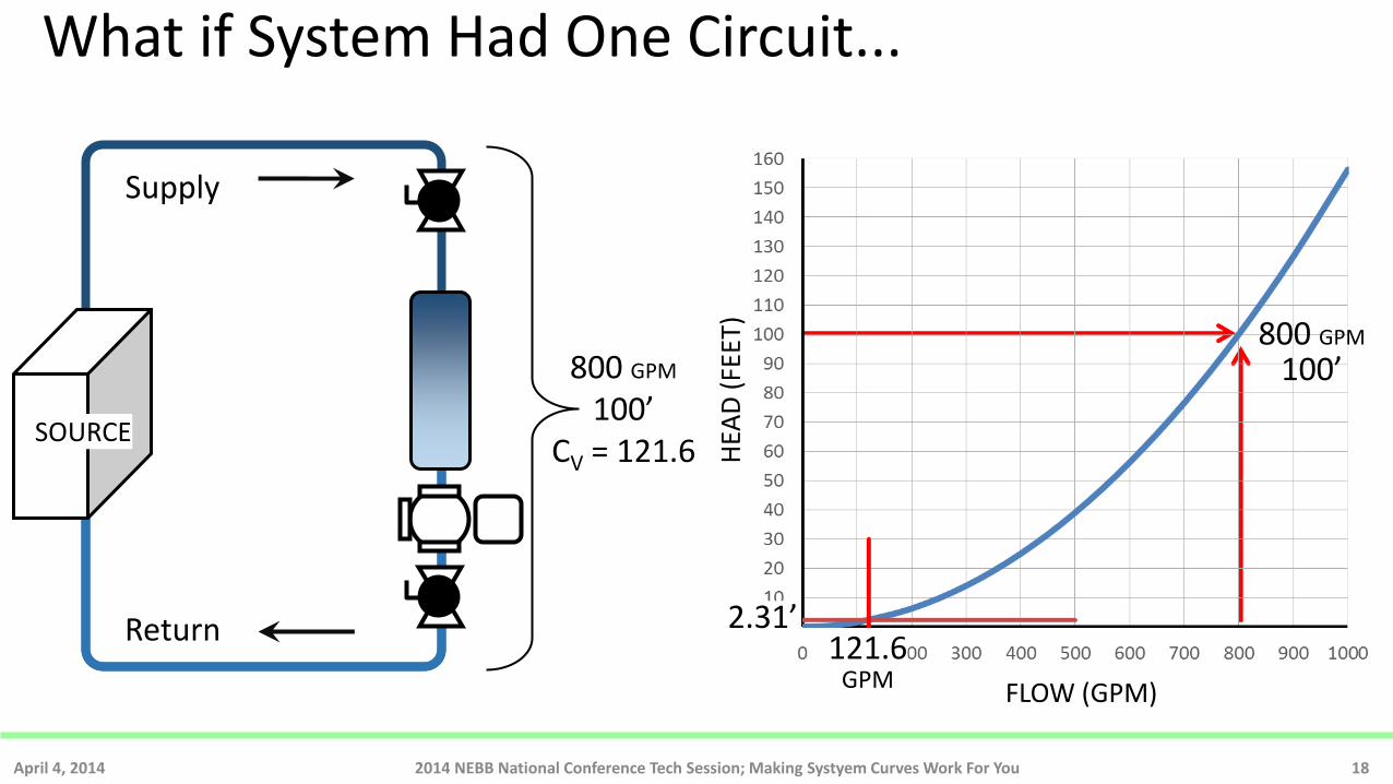
What if System Had One Circuit...
April 4, 2014 2014 NEBB National Conference Tech Session; Making Systyem Curves Work For You 18
800 GPM
100’ CV = 121.6
Supply
Return
SOURCE
HEA
D (
FEET
)
FLOW (GPM)
800 GPM
100’
2.31’ 121.6
GPM
So What?
• If we know that the CV is 121.6, we can predict what the flow will be at conditions other than 100’ when the system remains unchanged (valves open)
• If differential pressure were reduced across branch to 4 PSI, then flow would be 243.2 GPM
April 4, 2014 2014 NEBB National Conference Tech Session; Making Systyem Curves Work For You 19
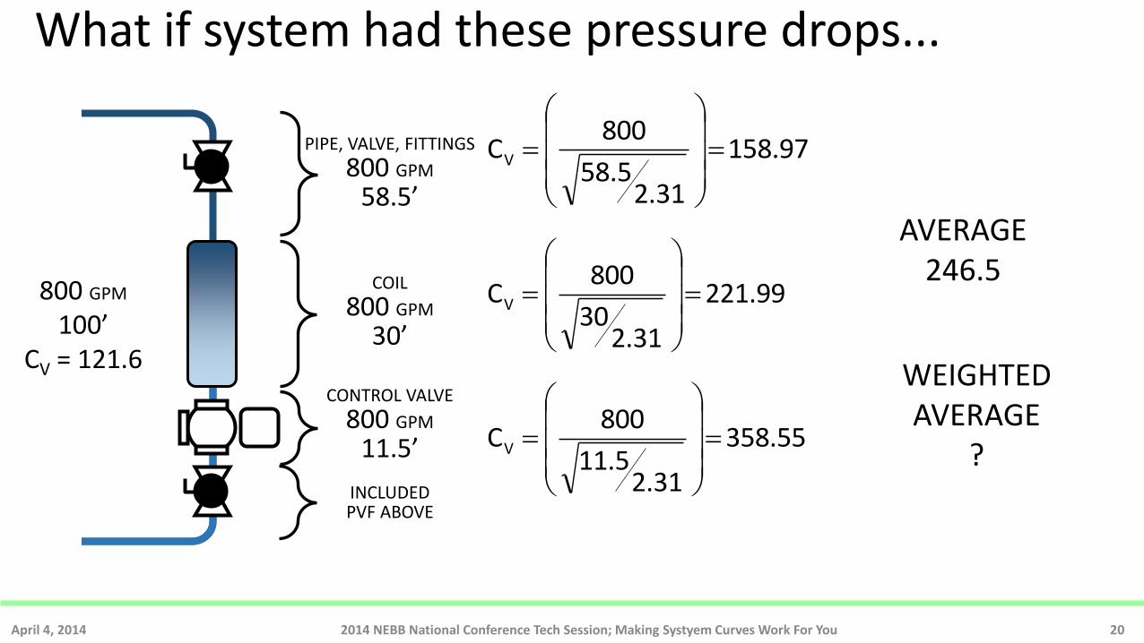
What if system had these pressure drops...
April 4, 2014 2014 NEBB National Conference Tech Session; Making Systyem Curves Work For You 20
PIPE, VALVE, FITTINGS
800 GPM
58.5’
800 GPM
100’ CV = 121.6
COIL
800 GPM
30’
CONTROL VALVE
800 GPM
11.5’
INCLUDED PVF ABOVE
158.97
2.3158.5
800CV
221.99
2.3130
800CV
358.55
2.3111.5
800CV
AVERAGE 246.5
WEIGHTED AVERAGE
?
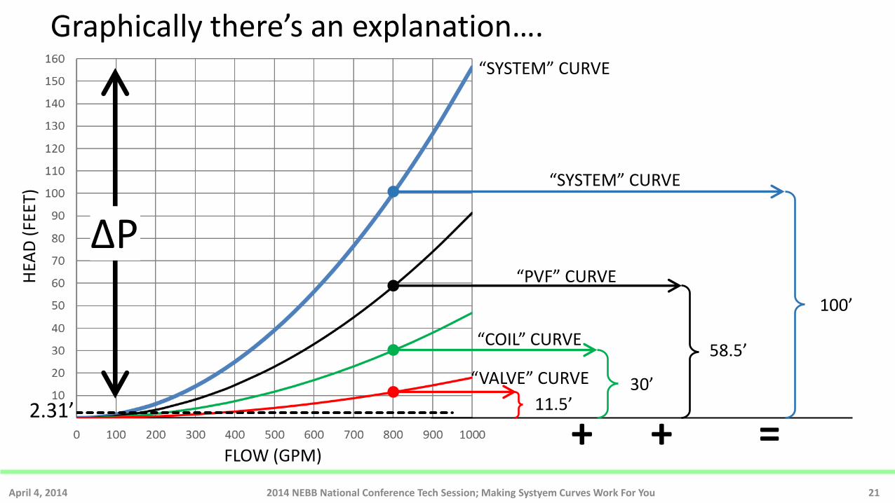
Graphically there’s an explanation….
April 4, 2014 2014 NEBB National Conference Tech Session; Making Systyem Curves Work For You 21
HEA
D (
FEET
)
FLOW (GPM)
2.31’
“SYSTEM” CURVE
“PVF” CURVE
“COIL” CURVE
“VALVE” CURVE
“SYSTEM” CURVE
100’
58.5’
30’ 11.5’
+ + =
ΔP
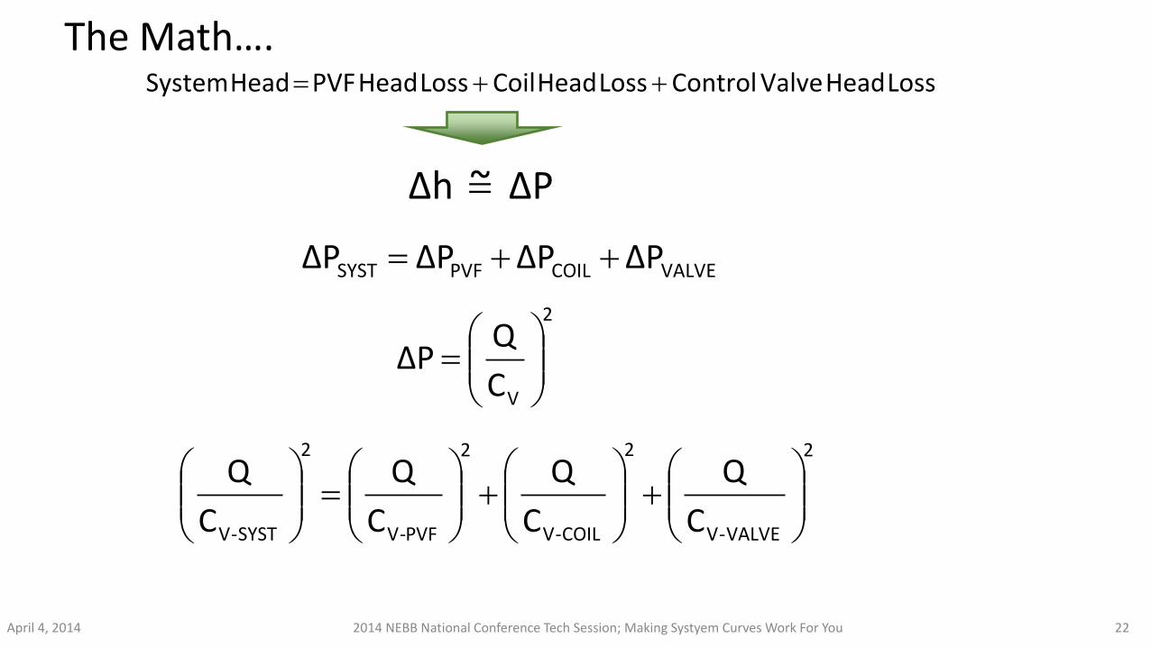
The Math….
April 4, 2014 2014 NEBB National Conference Tech Session; Making Systyem Curves Work For You 22
Loss Head Valve Control Loss Head Coil Loss Head PVF Head System
ΔP ~ Δh
VALVECOILPVFSYST ΔPΔPΔPΔP
2
VC
QΔP
2
VALVE-V
2
COIL-V
2
PVF-V
2
SYST-V C
Q
C
Q
C
Q
C
Q
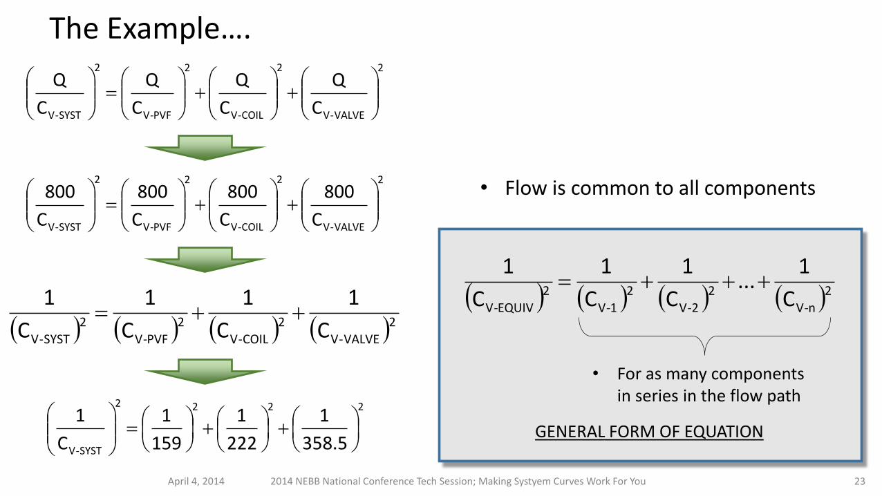
The Example….
April 4, 2014 2014 NEBB National Conference Tech Session; Making Systyem Curves Work For You 23
2
VALVE-V
2
COIL-V
2
PVF-V
2
SYST-V C
Q
C
Q
C
Q
C
Q
2
VALVE-V
2
COIL-V
2
PVF-V
2
SYST-V C
800
C
800
C
800
C
800
2
VALVE-V
2
COIL-V
2
PVF-V
2
SYST-V C
1
C
1
C
1
C
1
2222
SYST-V 358.5
1
222
1
159
1
C
1
• Flow is common to all components
2
n-V
2
2-V
2
1-V
2
EQUIV-V C
1...
C
1
C
1
C
1
GENERAL FORM OF EQUATION
• For as many components in series in the flow path
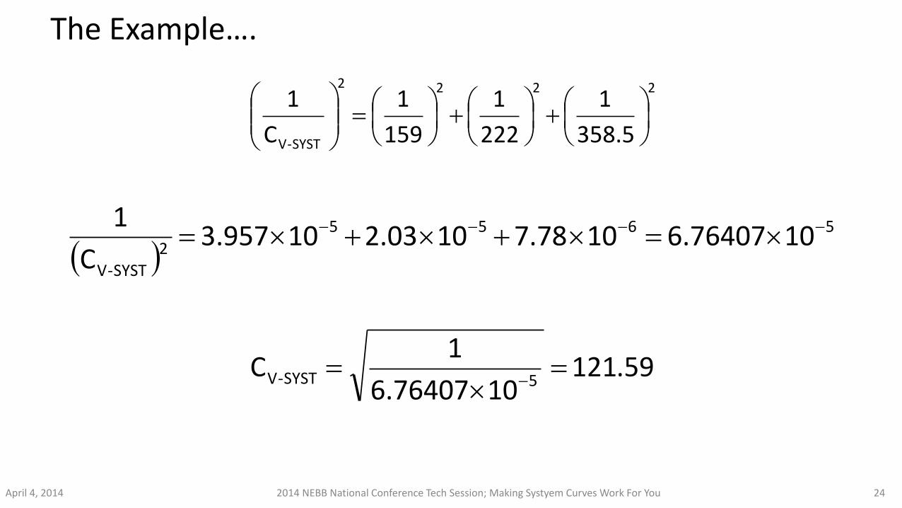
The Example….
April 4, 2014 2014 NEBB National Conference Tech Session; Making Systyem Curves Work For You 24
2222
SYST-V 358.5
1
222
1
159
1
C
1
5655
2
SYST-V
106.76407107.78102.03103.957C
1
59.121106.76407
1C
5SYST-V

Notes
• Every component with a known flow and head loss can have a flow coefficient implied • Pipe; Size, , FlowFriction Loss / Length, Length of Pipe • Coils, Fixed Position Valves, Strainers
• Non-variable devices have a constant flow coefficient • Composite device coefficient may be defined, grouping NV devices
• Variable devices (Flow Control Valves) have a unique flow coefficient for each position • Calculating system flow coefficient for each variable device position with the
device coefficient shows the ability of the device to adjust flow (Valve Authority)
April 4, 2014 2014 NEBB National Conference Tech Session; Making Systyem Curves Work For You 25
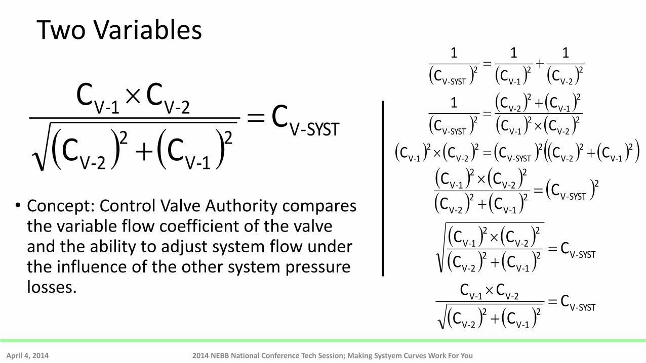
Two Variables
• Concept: Control Valve Authority compares the variable flow coefficient of the valve and the ability to adjust system flow under the influence of the other system pressure losses.
April 4, 2014 2014 NEBB National Conference Tech Session; Making Systyem Curves Work For You
21-V
22-V
2SYST-V
22-V
21-V
22-V
21-V
2
1-V
2
2-V2
SYST-V
2
2-V
2
1-V
2
SYST-V
CCCCC
CC
CC
C
1
C
1
C
1
C
1
SYST-V2
1-V
2
2-V
2-V1-V
SYST-V2
1-V
2
2-V
2
2-V
2
1-V
2
SYST-V2
1-V
2
2-V
2
2-V
2
1-V
CCC
CC
CCC
CC
CCC
CC
SYST-V2
1-V
2
2-V
2-V1-V CCC
CC
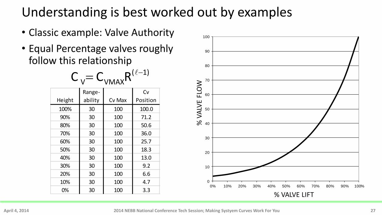
Understanding is best worked out by examples
• Classic example: Valve Authority
• Equal Percentage valves roughly follow this relationship
April 4, 2014 2014 NEBB National Conference Tech Session; Making Systyem Curves Work For You 27
Height
Range-
ability Cv Max
Cv
Position
100% 30 100 100.0
90% 30 100 71.2
80% 30 100 50.6
70% 30 100 36.0
60% 30 100 25.7
50% 30 100 18.3
40% 30 100 13.0
30% 30 100 9.2
20% 30 100 6.6
10% 30 100 4.7
0% 30 100 3.3
0
10
20
30
40
50
60
70
80
90
100
0% 10% 20% 30% 40% 50% 60% 70% 80% 90% 100%
% V
ALV
E FL
OW
% VALVE LIFT
1)(VMAXV RCC
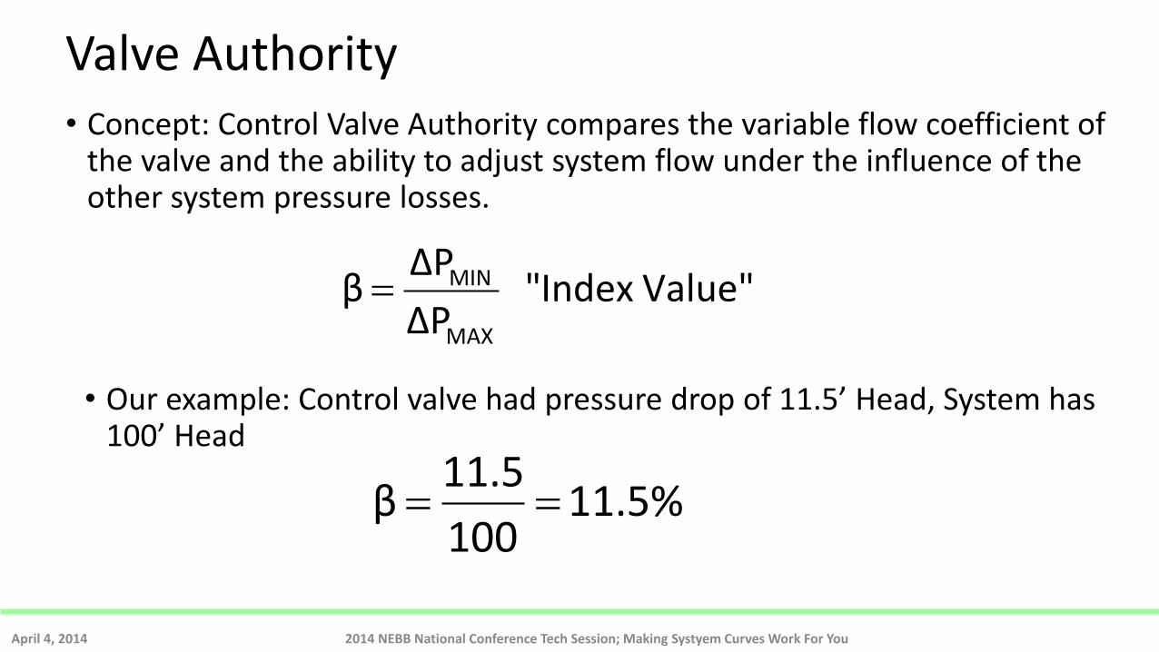
Valve Authority • Concept: Control Valve Authority compares the variable flow coefficient of
the valve and the ability to adjust system flow under the influence of the other system pressure losses.
April 4, 2014 2014 NEBB National Conference Tech Session; Making Systyem Curves Work For You
Value" Index" ΔP
ΔPβ
MAX
MIN
• Our example: Control valve had pressure drop of 11.5’ Head, System has 100’ Head
11.5%100
11.5β
April 4, 2014 2014 NEBB National Conference Tech Session; Making Systyem Curves Work For You 29
0%
10%
20%
30%
40%
50%
60%
70%
80%
90%
100%
0% 10% 20% 30% 40% 50% 60% 70% 80% 90% 100%
% V
ALV
E FL
OW
% VALVE LIFT
Height Range-ability Cv Max Cv Position
Modifed Cv
System Components System Cv
Percent Valve
Percent System
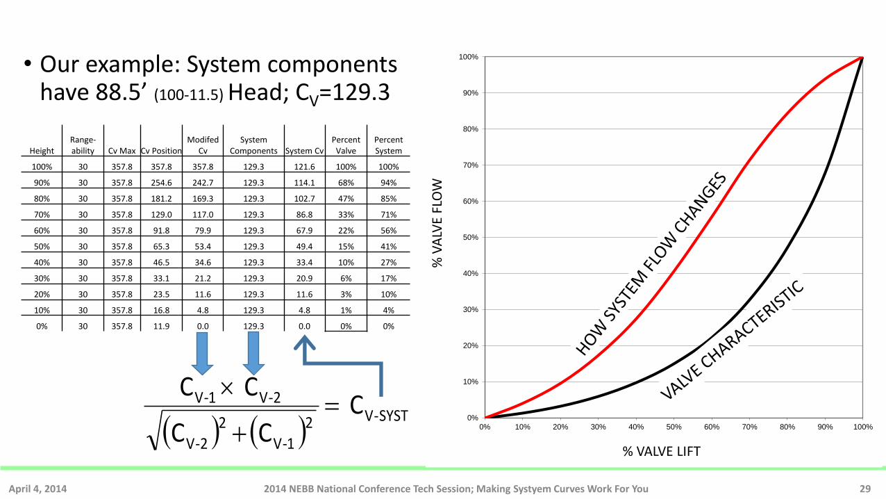
100% 30 357.8 357.8 357.8 129.3 121.6 100% 100%
90% 30 357.8 254.6 242.7 129.3 114.1 68% 94%
80% 30 357.8 181.2 169.3 129.3 102.7 47% 85%
70% 30 357.8 129.0 117.0 129.3 86.8 33% 71%
60% 30 357.8 91.8 79.9 129.3 67.9 22% 56%
50% 30 357.8 65.3 53.4 129.3 49.4 15% 41%
40% 30 357.8 46.5 34.6 129.3 33.4 10% 27%
30% 30 357.8 33.1 21.2 129.3 20.9 6% 17%
20% 30 357.8 23.5 11.6 129.3 11.6 3% 10%
10% 30 357.8 16.8 4.8 129.3 4.8 1% 4%
0% 30 357.8 11.9 0.0 129.3 0.0 0% 0%
• Our example: System components have 88.5’ (100-11.5) Head; CV=129.3
SYST-V2
1-V
2
2-V
2-V1-V C CC
C C

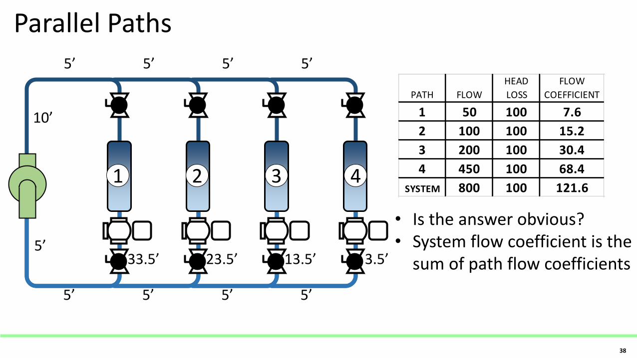
Parallel Paths
37
4 3 2 1
• System 800 GPM @ 100’ Head
• All circuits are proportionally balanced • All circuits have same
head loss (100’) • Distribution losses as shown
• Coil & Valve same as previous example
5’ 5’ 5’ 5’
5’ 5’ 5’ 5’
5’
10’
13.5’ 23.5’ 33.5’ 3.5’
Parallel Paths
38
4 3 2 1
5’ 5’ 5’ 5’
5’ 5’ 5’ 5’
5’
10’
13.5’ 23.5’ 33.5’ 3.5’
PATH FLOW
HEAD
LOSS
FLOW
COEFFICIENT
1 50 100 7.6
2 100 100 15.2
3 200 100 30.4
4 450 100 68.4
SYSTEM 800 100 121.6
• Is the answer obvious? • System flow coefficient is the
sum of path flow coefficients
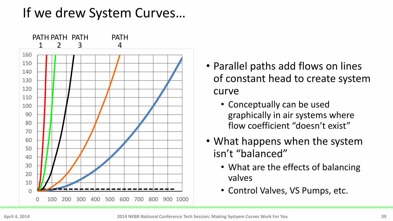
If we drew System Curves…
• Parallel paths add flows on lines of constant head to create system curve • Conceptually can be used
graphically in air systems where flow coefficient “doesn’t exist”
• What happens when the system isn’t “balanced” • What are the effects of balancing
valves
• Control Valves, VS Pumps, etc.
April 4, 2014 2014 NEBB National Conference Tech Session; Making Systyem Curves Work For You 39
0
10
20
30
40
50
60
70
80
90
100
110
120
130
140
150
160
0 100 200 300 400 500 600 700 800 900 1000
PATH 1
PATH 2
PATH 3
PATH 4
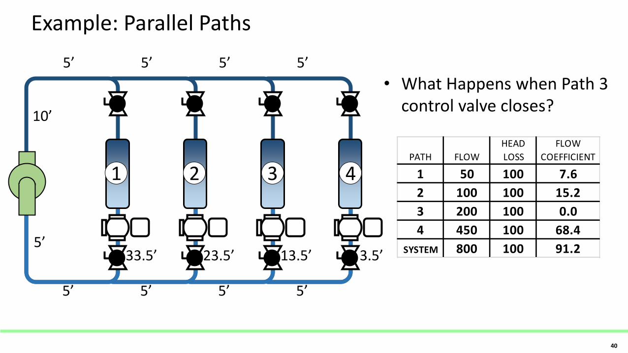
Example: Parallel Paths
40
4 3 2 1
5’ 5’ 5’ 5’
5’ 5’ 5’ 5’
5’
10’
13.5’ 23.5’ 33.5’ 3.5’
PATH FLOW
HEAD
LOSS
FLOW
COEFFICIENT
1 50 100 7.6
2 100 100 15.2
3 200 100 0.0
4 450 100 68.4
SYSTEM 800 100 91.2
• What Happens when Path 3 control valve closes?
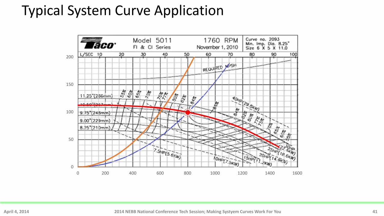
Typical System Curve Application
April 4, 2014 2014 NEBB National Conference Tech Session; Making Systyem Curves Work For You 41
0
50
100
150
200
0 200 400 600 800 1000 1200 1400 1600
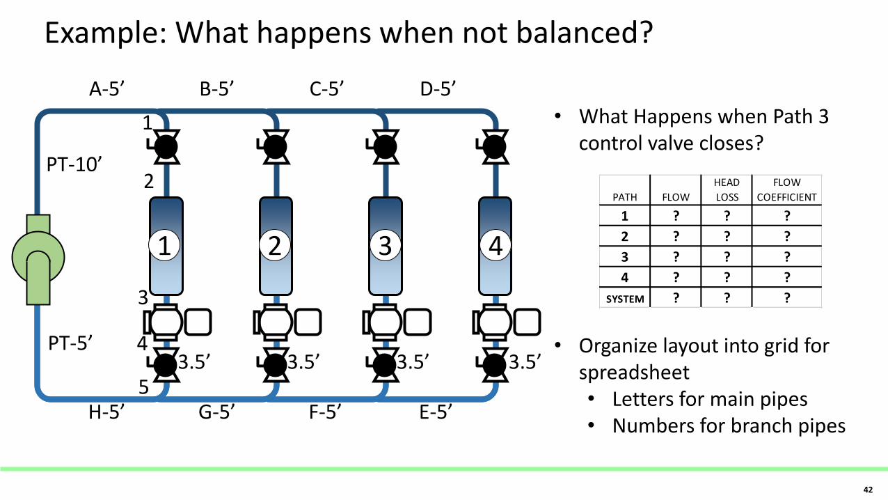
Example: What happens when not balanced?
42
4 3 2 1
A-5’ B-5’ C-5’ D-5’
H-5’ G-5’ F-5’ E-5’
PT-5’
PT-10’
3.5’ 3.5’ 3.5’ 3.5’
PATH FLOW
HEAD
LOSS
FLOW
COEFFICIENT
1 ? ? ?
2 ? ? ?
3 ? ? ?
4 ? ? ?
SYSTEM ? ? ?
• What Happens when Path 3 control valve closes?
1
2
3
4
5
• Organize layout into grid for spreadsheet • Letters for main pipes • Numbers for branch pipes
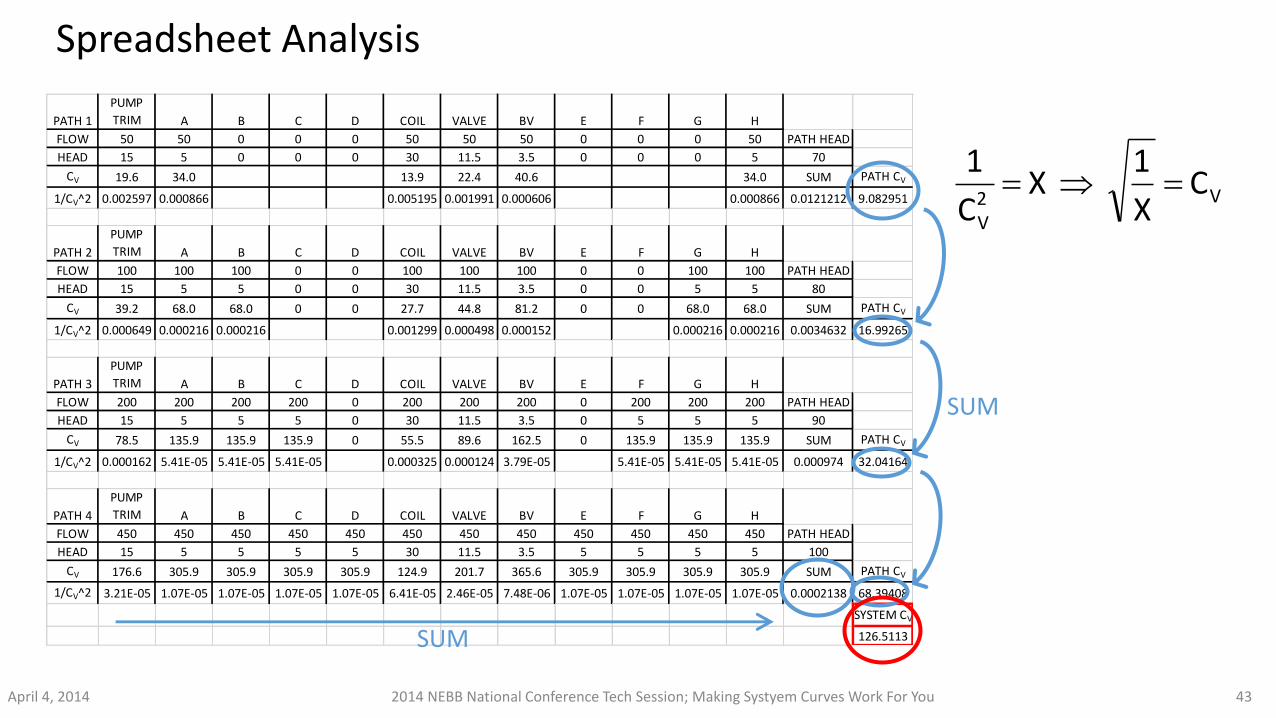
Spreadsheet Analysis
April 4, 2014 2014 NEBB National Conference Tech Session; Making Systyem Curves Work For You 43
PATH 1
PUMP
TRIM A B C D COIL VALVE BV E F G H
FLOW 50 50 0 0 0 50 50 50 0 0 0 50 PATH HEAD
HEAD 15 5 0 0 0 30 11.5 3.5 0 0 0 5 70
CV 19.6 34.0 13.9 22.4 40.6 34.0 SUM PATH CV
1/CV^2 0.002597 0.000866 0.005195 0.001991 0.000606 0.000866 0.0121212 9.082951
PATH 2
PUMP
TRIM A B C D COIL VALVE BV E F G H
FLOW 100 100 100 0 0 100 100 100 0 0 100 100 PATH HEAD
HEAD 15 5 5 0 0 30 11.5 3.5 0 0 5 5 80
CV 39.2 68.0 68.0 0 0 27.7 44.8 81.2 0 0 68.0 68.0 SUM PATH CV
1/CV^2 0.000649 0.000216 0.000216 0.001299 0.000498 0.000152 0.000216 0.000216 0.0034632 16.99265
PATH 3
PUMP
TRIM A B C D COIL VALVE BV E F G H
FLOW 200 200 200 200 0 200 200 200 0 200 200 200 PATH HEAD
HEAD 15 5 5 5 0 30 11.5 3.5 0 5 5 5 90
CV 78.5 135.9 135.9 135.9 0 55.5 89.6 162.5 0 135.9 135.9 135.9 SUM PATH CV
1/CV^2 0.000162 5.41E-05 5.41E-05 5.41E-05 0.000325 0.000124 3.79E-05 5.41E-05 5.41E-05 5.41E-05 0.000974 32.04164
PATH 4
PUMP
TRIM A B C D COIL VALVE BV E F G H
FLOW 450 450 450 450 450 450 450 450 450 450 450 450 PATH HEAD
HEAD 15 5 5 5 5 30 11.5 3.5 5 5 5 5 100
CV 176.6 305.9 305.9 305.9 305.9 124.9 201.7 365.6 305.9 305.9 305.9 305.9 SUM PATH CV
1/CV^2 3.21E-05 1.07E-05 1.07E-05 1.07E-05 1.07E-05 6.41E-05 2.46E-05 7.48E-06 1.07E-05 1.07E-05 1.07E-05 1.07E-05 0.0002138 68.39408
SYSTEM CV
126.5113SUM
V2V
CX
1 X
C
1
SUM
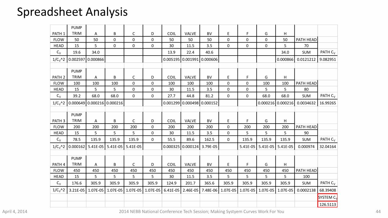
Spreadsheet Analysis
April 4, 2014 2014 NEBB National Conference Tech Session; Making Systyem Curves Work For You 44
PATH 1
PUMP
TRIM A B C D COIL VALVE BV E F G H
FLOW 50 50 0 0 0 50 50 50 0 0 0 50 PATH HEAD
HEAD 15 5 0 0 0 30 11.5 3.5 0 0 0 5 70
CV 19.6 34.0 13.9 22.4 40.6 34.0 SUM PATH CV
1/CV^2 0.002597 0.000866 0.005195 0.001991 0.000606 0.000866 0.0121212 9.082951
PATH 2
PUMP
TRIM A B C D COIL VALVE BV E F G H
FLOW 100 100 100 0 0 100 100 100 0 0 100 100 PATH HEAD
HEAD 15 5 5 0 0 30 11.5 3.5 0 0 5 5 80
CV 39.2 68.0 68.0 0 0 27.7 44.8 81.2 0 0 68.0 68.0 SUM PATH CV
1/CV^2 0.000649 0.000216 0.000216 0.001299 0.000498 0.000152 0.000216 0.000216 0.0034632 16.99265
PATH 3
PUMP
TRIM A B C D COIL VALVE BV E F G H
FLOW 200 200 200 200 0 200 200 200 0 200 200 200 PATH HEAD
HEAD 15 5 5 5 0 30 11.5 3.5 0 5 5 5 90
CV 78.5 135.9 135.9 135.9 0 55.5 89.6 162.5 0 135.9 135.9 135.9 SUM PATH CV
1/CV^2 0.000162 5.41E-05 5.41E-05 5.41E-05 0.000325 0.000124 3.79E-05 5.41E-05 5.41E-05 5.41E-05 0.000974 32.04164
PATH 4
PUMP
TRIM A B C D COIL VALVE BV E F G H
FLOW 450 450 450 450 450 450 450 450 450 450 450 450 PATH HEAD
HEAD 15 5 5 5 5 30 11.5 3.5 5 5 5 5 100
CV 176.6 305.9 305.9 305.9 305.9 124.9 201.7 365.6 305.9 305.9 305.9 305.9 SUM PATH CV
1/CV^2 3.21E-05 1.07E-05 1.07E-05 1.07E-05 1.07E-05 6.41E-05 2.46E-05 7.48E-06 1.07E-05 1.07E-05 1.07E-05 1.07E-05 0.0002138 68.39408
SYSTEM CV
126.5113
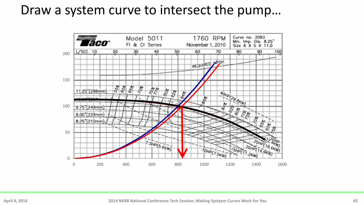
Draw a system curve to intersect the pump…
April 4, 2014 2014 NEBB National Conference Tech Session; Making Systyem Curves Work For You 45
0
50
100
150
200
0 200 400 600 800 1000 1200 1400 1600
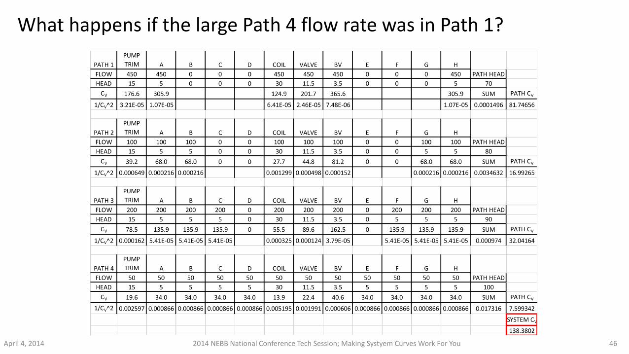
What happens if the large Path 4 flow rate was in Path 1?
April 4, 2014 2014 NEBB National Conference Tech Session; Making Systyem Curves Work For You 46
PATH 1
PUMP
TRIM A B C D COIL VALVE BV E F G H
FLOW 450 450 0 0 0 450 450 450 0 0 0 450 PATH HEAD
HEAD 15 5 0 0 0 30 11.5 3.5 0 0 0 5 70
CV 176.6 305.9 124.9 201.7 365.6 305.9 SUM PATH CV
1/CV^2 3.21E-05 1.07E-05 6.41E-05 2.46E-05 7.48E-06 1.07E-05 0.0001496 81.74656
PATH 2
PUMP
TRIM A B C D COIL VALVE BV E F G H
FLOW 100 100 100 0 0 100 100 100 0 0 100 100 PATH HEAD
HEAD 15 5 5 0 0 30 11.5 3.5 0 0 5 5 80
CV 39.2 68.0 68.0 0 0 27.7 44.8 81.2 0 0 68.0 68.0 SUM PATH CV
1/CV^2 0.000649 0.000216 0.000216 0.001299 0.000498 0.000152 0.000216 0.000216 0.0034632 16.99265
PATH 3
PUMP
TRIM A B C D COIL VALVE BV E F G H
FLOW 200 200 200 200 0 200 200 200 0 200 200 200 PATH HEAD
HEAD 15 5 5 5 0 30 11.5 3.5 0 5 5 5 90
CV 78.5 135.9 135.9 135.9 0 55.5 89.6 162.5 0 135.9 135.9 135.9 SUM PATH CV
1/CV^2 0.000162 5.41E-05 5.41E-05 5.41E-05 0.000325 0.000124 3.79E-05 5.41E-05 5.41E-05 5.41E-05 0.000974 32.04164
PATH 4
PUMP
TRIM A B C D COIL VALVE BV E F G H
FLOW 50 50 50 50 50 50 50 50 50 50 50 50 PATH HEAD
HEAD 15 5 5 5 5 30 11.5 3.5 5 5 5 5 100
CV 19.6 34.0 34.0 34.0 34.0 13.9 22.4 40.6 34.0 34.0 34.0 34.0 SUM PATH CV
1/CV^2 0.002597 0.000866 0.000866 0.000866 0.000866 0.005195 0.001991 0.000606 0.000866 0.000866 0.000866 0.000866 0.017316 7.599342
SYSTEM CV
138.3802
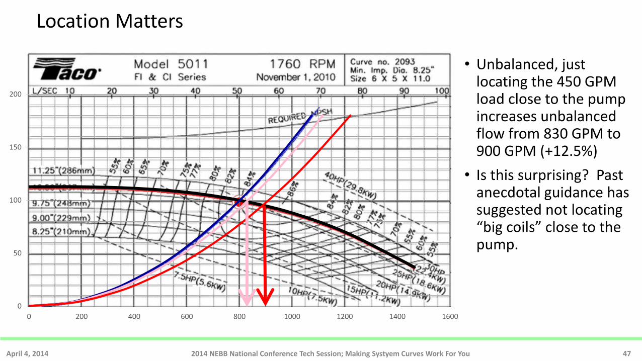
Location Matters
• Unbalanced, just locating the 450 GPM load close to the pump increases unbalanced flow from 830 GPM to 900 GPM (+12.5%)
• Is this surprising? Past anecdotal guidance has suggested not locating “big coils” close to the pump.
April 4, 2014 2014 NEBB National Conference Tech Session; Making Systyem Curves Work For You 47
0
50
100
150
200
0 200 400 600 800 1000 1200 1400 1600
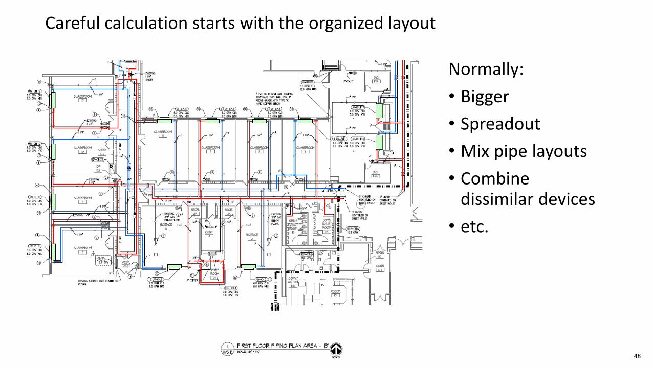
Careful calculation starts with the organized layout
Normally:
• Bigger
• Spreadout
• Mix pipe layouts
• Combine dissimilar devices
• etc.
48
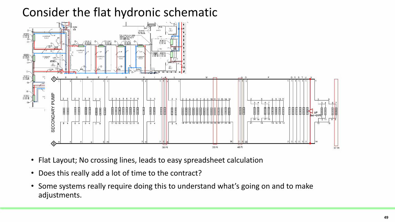
Consider the flat hydronic schematic
• Flat Layout; No crossing lines, leads to easy spreadsheet calculation
• Does this really add a lot of time to the contract?
• Some systems really require doing this to understand what’s going on and to make adjustments.
49
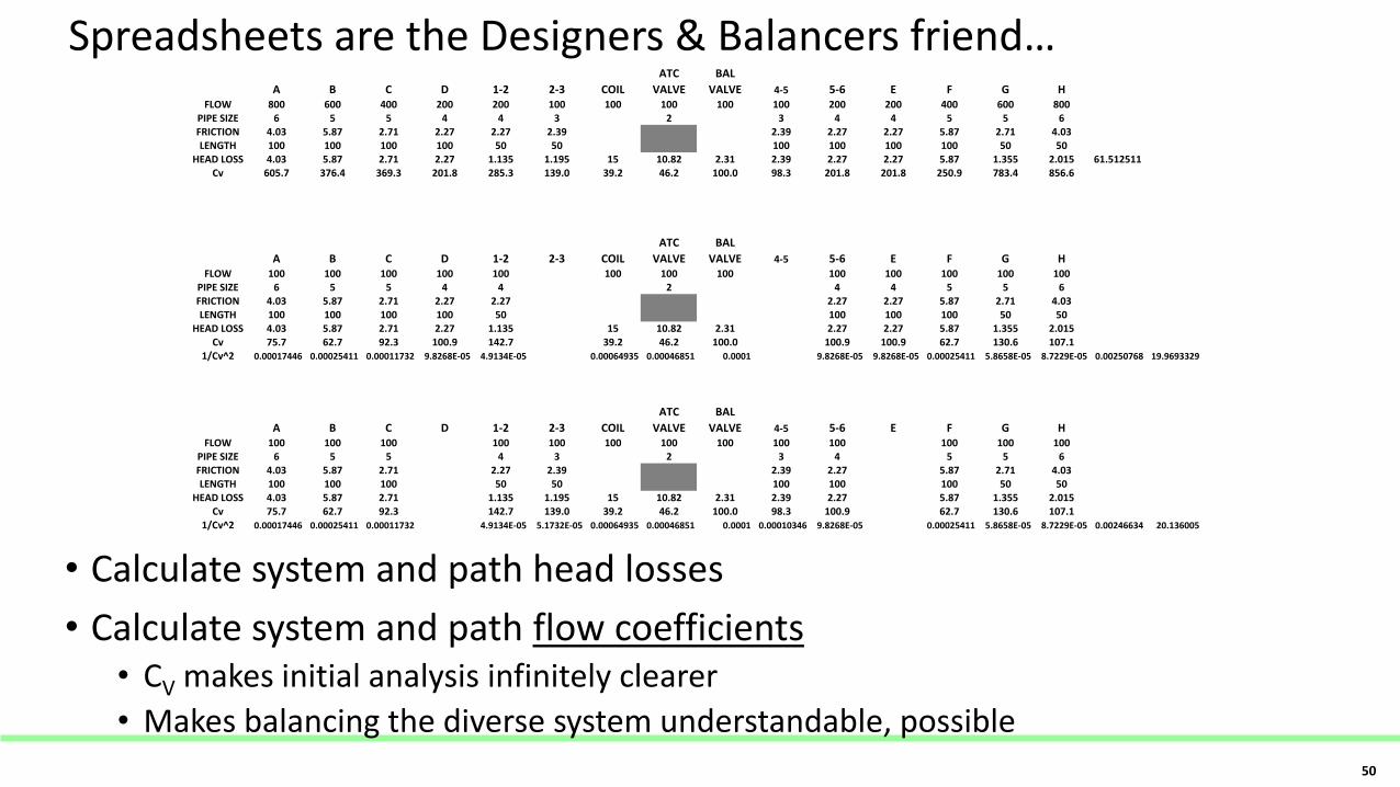
Spreadsheets are the Designers & Balancers friend…
• Calculate system and path head losses
• Calculate system and path flow coefficients • CV makes initial analysis infinitely clearer
• Makes balancing the diverse system understandable, possible
A B C D 1-2 2-3 COIL
ATC
VALVE
BAL
VALVE 4-5 5-6 E F G HFLOW 800 600 400 200 200 100 100 100 100 100 200 200 400 600 800
PIPE SIZE 6 5 5 4 4 3 2 3 4 4 5 5 6FRICTION 4.03 5.87 2.71 2.27 2.27 2.39 2.39 2.27 2.27 5.87 2.71 4.03LENGTH 100 100 100 100 50 50 100 100 100 100 50 50
HEAD LOSS 4.03 5.87 2.71 2.27 1.135 1.195 15 10.82 2.31 2.39 2.27 2.27 5.87 1.355 2.015 61.512511Cv 605.7 376.4 369.3 201.8 285.3 139.0 39.2 46.2 100.0 98.3 201.8 201.8 250.9 783.4 856.6
A B C D 1-2 2-3 COIL
ATC
VALVE
BAL
VALVE 4-5 5-6 E F G HFLOW 100 100 100 100 100 100 100 100 100 100 100 100 100
PIPE SIZE 6 5 5 4 4 2 4 4 5 5 6FRICTION 4.03 5.87 2.71 2.27 2.27 2.27 2.27 5.87 2.71 4.03LENGTH 100 100 100 100 50 100 100 100 50 50
HEAD LOSS 4.03 5.87 2.71 2.27 1.135 15 10.82 2.31 2.27 2.27 5.87 1.355 2.015Cv 75.7 62.7 92.3 100.9 142.7 39.2 46.2 100.0 100.9 100.9 62.7 130.6 107.1
1/Cv^2 0.00017446 0.00025411 0.00011732 9.8268E-05 4.9134E-05 0.00064935 0.00046851 0.0001 9.8268E-05 9.8268E-05 0.00025411 5.8658E-05 8.7229E-05 0.00250768 19.9693329
A B C D 1-2 2-3 COIL
ATC
VALVE
BAL
VALVE 4-5 5-6 E F G HFLOW 100 100 100 100 100 100 100 100 100 100 100 100 100
PIPE SIZE 6 5 5 4 3 2 3 4 5 5 6FRICTION 4.03 5.87 2.71 2.27 2.39 2.39 2.27 5.87 2.71 4.03LENGTH 100 100 100 50 50 100 100 100 50 50
HEAD LOSS 4.03 5.87 2.71 1.135 1.195 15 10.82 2.31 2.39 2.27 5.87 1.355 2.015Cv 75.7 62.7 92.3 142.7 139.0 39.2 46.2 100.0 98.3 100.9 62.7 130.6 107.1
1/Cv^2 0.00017446 0.00025411 0.00011732 4.9134E-05 5.1732E-05 0.00064935 0.00046851 0.0001 0.00010346 9.8268E-05 0.00025411 5.8658E-05 8.7229E-05 0.00246634 20.136005
50
A comment on Calculation
• Designers have an ethical responsibility to calculate the hydronic system… • ASHRAE Standard 111 TAB requires designers to forward their calculations to the
TAB agency
• Balancers don’t feel paid to calculate system hydraulics • It’s not that hard! It doesn’t need to be that precise!
• Balancers are paid to provide a report and test data, part of which are data collected from submittals and design schedules…
• A day or two in the office probably saves a week or more in the field feeling mystified
51
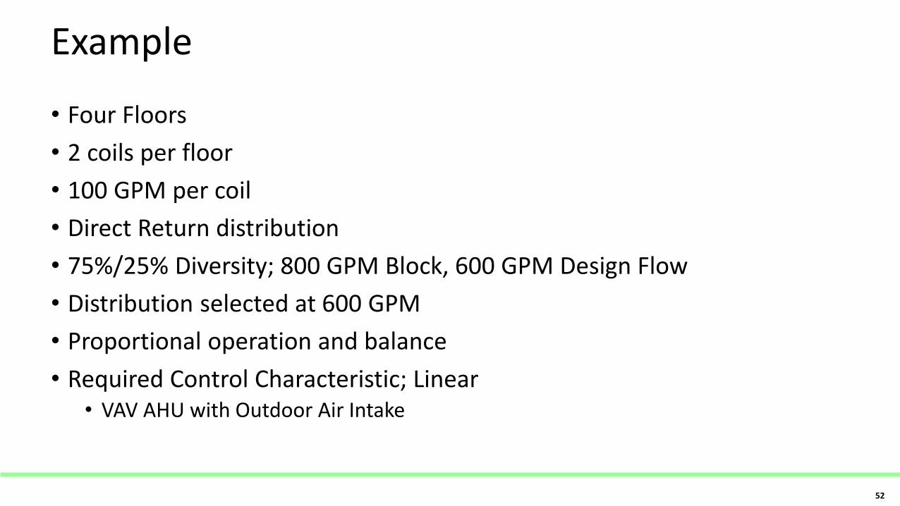
Example
• Four Floors
• 2 coils per floor
• 100 GPM per coil
• Direct Return distribution
• 75%/25% Diversity; 800 GPM Block, 600 GPM Design Flow
• Distribution selected at 600 GPM
• Proportional operation and balance
• Required Control Characteristic; Linear • VAV AHU with Outdoor Air Intake
52
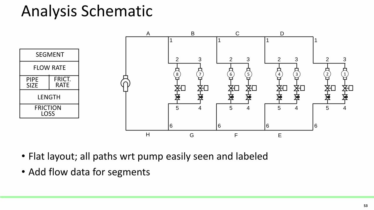
Analysis Schematic
• Flat layout; all paths wrt pump easily seen and labeled
• Add flow data for segments
53
FLOW RATE
PIPE SIZE
FRICT. RATE
LENGTH
FRICTION LOSS
SEGMENT
A B C D
1
2 3
5 4
6
1
2 3
5 4
6
1
2 3
5 4
6
1
2 3
5 4
6
G F E
1 2 3 4 5 6 7 8
H
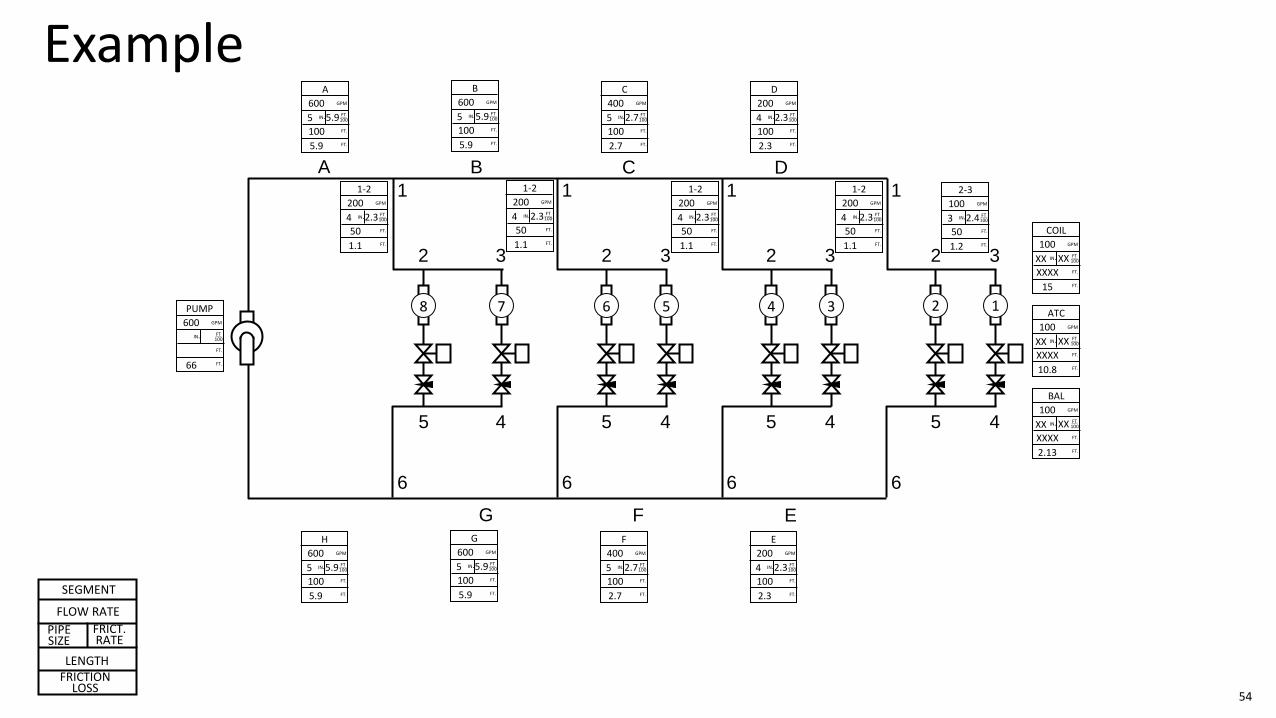
Example
54
A B C D
1
2 3
5 4
6
1
2 3
5 4
6
1
2 3
5 4
6
1
2 3
5 4
6
G F E
GPM
FT.
FT.
IN. FT 100
600
5 5.9
100
5.9
A GPM
FT.
FT.
IN. FT 100
600
5 5.9
100
5.9
B GPM
FT.
FT.
IN. FT 100
400
5 2.7
100
2.7
C GPM
FT.
FT.
IN. FT 100
200
4 2.3
100
2.3
D
GPM
FT.
FT.
IN. FT 100
200
4 2.3
50
1.1
1-2 GPM
FT.
FT.
IN. FT 100
200
4 2.3
50
1.1
1-2 GPM
FT.
FT.
IN. FT 100
200
4 2.3
50
1.1
1-2 GPM
FT.
FT.
IN. FT 100
200
4 2.3
50
1.1
1-2
GPM
FT.
FT.
IN. FT 100
100
XX XX
XXXX
15
COIL
GPM
FT.
FT.
IN. FT 100
100
XX XX
XXXX
10.8
ATC
GPM
FT.
FT.
IN. FT 100
100
XX XX
XXXX
2.13
BAL
1 2 3 4 5 6 7 8
GPM
FT.
FT.
IN. FT 100
100
3 2.4
50
1.2
2-3
GPM
FT.
FT.
IN. FT 100
600
5 5.9
100
5.9
H GPM
FT.
FT.
IN. FT 100
600
5 5.9
100
5.9
G GPM
FT.
FT.
IN. FT 100
400
5 2.7
100
2.7
F GPM
FT.
FT.
IN. FT 100
200
4 2.3
100
2.3
E
GPM
FT.
FT.
IN. FT 100
600
66
PUMP
FLOW RATE
PIPE SIZE
FRICT. RATE
LENGTH FRICTION
LOSS
SEGMENT
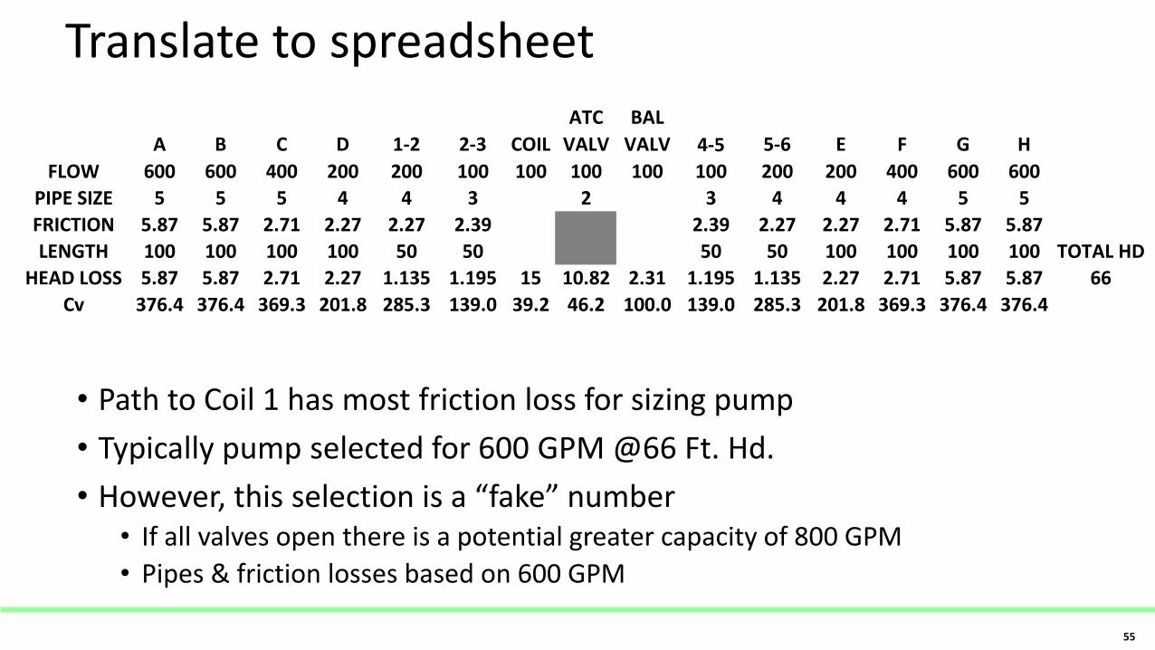
Translate to spreadsheet
• Path to Coil 1 has most friction loss for sizing pump
• Typically pump selected for 600 GPM @66 Ft. Hd.
• However, this selection is a “fake” number • If all valves open there is a potential greater capacity of 800 GPM
• Pipes & friction losses based on 600 GPM
A B C D 1-2 2-3 COIL
ATC
VALV
BAL
VALV 4-5 5-6 E F G H
FLOW 600 600 400 200 200 100 100 100 100 100 200 200 400 600 600
PIPE SIZE 5 5 5 4 4 3 2 3 4 4 4 5 5
FRICTION 5.87 5.87 2.71 2.27 2.27 2.39 2.39 2.27 2.27 2.71 5.87 5.87
LENGTH 100 100 100 100 50 50 50 50 100 100 100 100 TOTAL HD
HEAD LOSS 5.87 5.87 2.71 2.27 1.135 1.195 15 10.82 2.31 1.195 1.135 2.27 2.71 5.87 5.87 66
Cv 376.4 376.4 369.3 201.8 285.3 139.0 39.2 46.2 100.0 139.0 285.3 201.8 369.3 376.4 376.4
55

Pump Selection
FLOW (USGPM)
HEA
D (
FEET
)
56
Issue; Do you have to go to the field and measure?
• No (sort of)
• Review application of System Flow Coefficient theory
57
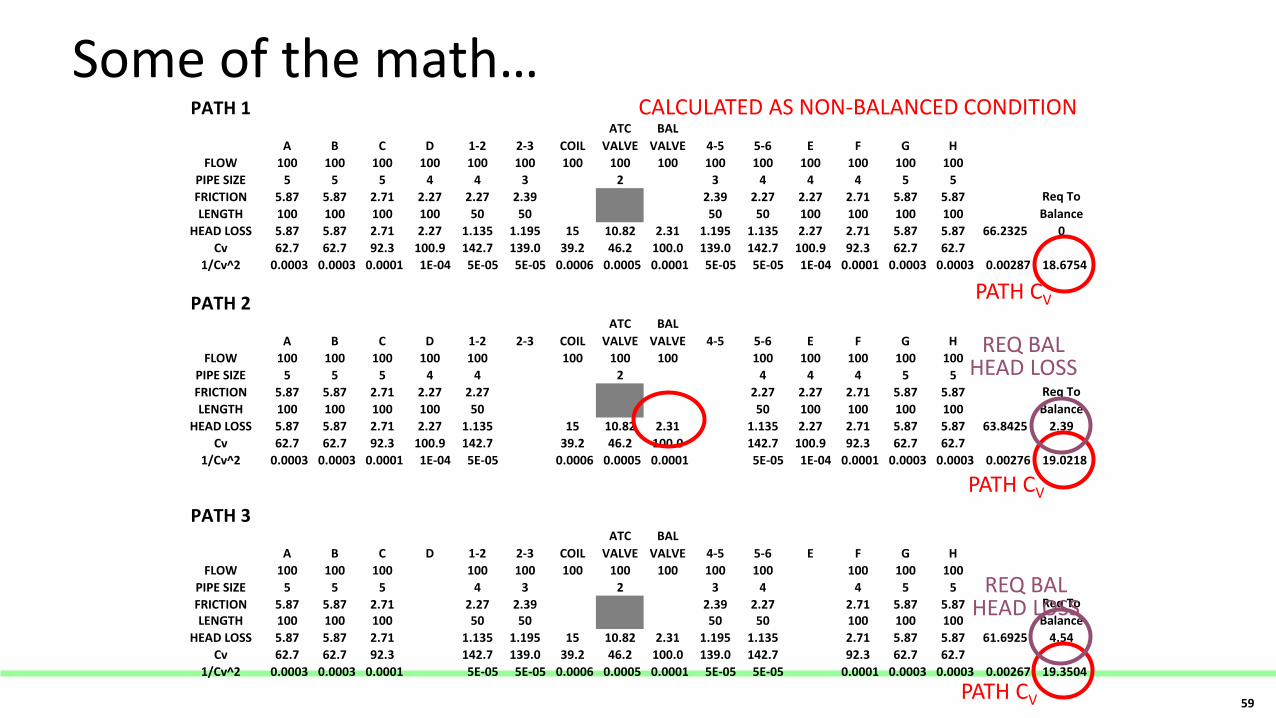
Some of the math… PATH 1
A B C D 1-2 2-3 COIL
ATC
VALVE
BAL
VALVE 4-5 5-6 E F G H
FLOW 100 100 100 100 100 100 100 100 100 100 100 100 100 100 100
PIPE SIZE 5 5 5 4 4 3 2 3 4 4 4 5 5
FRICTION 5.87 5.87 2.71 2.27 2.27 2.39 2.39 2.27 2.27 2.71 5.87 5.87
LENGTH 100 100 100 100 50 50 50 50 100 100 100 100
HEAD LOSS 5.87 5.87 2.71 2.27 1.135 1.195 15 10.82 2.31 1.195 1.135 2.27 2.71 5.87 5.87 66.2325 0
Cv 62.7 62.7 92.3 100.9 142.7 139.0 39.2 46.2 100.0 139.0 142.7 100.9 92.3 62.7 62.7
1/Cv^2 0.0003 0.0003 0.0001 1E-04 5E-05 5E-05 0.0006 0.0005 0.0001 5E-05 5E-05 1E-04 0.0001 0.0003 0.0003 0.00287 18.6754
PATH 2
A B C D 1-2 2-3 COIL
ATC
VALVE
BAL
VALVE 4-5 5-6 E F G H
FLOW 100 100 100 100 100 100 100 100 100 100 100 100 100
PIPE SIZE 5 5 5 4 4 2 4 4 4 5 5
FRICTION 5.87 5.87 2.71 2.27 2.27 2.27 2.27 2.71 5.87 5.87
LENGTH 100 100 100 100 50 50 100 100 100 100
HEAD LOSS 5.87 5.87 2.71 2.27 1.135 15 10.82 2.31 1.135 2.27 2.71 5.87 5.87 63.8425 2.39
Cv 62.7 62.7 92.3 100.9 142.7 39.2 46.2 100.0 142.7 100.9 92.3 62.7 62.7
1/Cv^2 0.0003 0.0003 0.0001 1E-04 5E-05 0.0006 0.0005 0.0001 5E-05 1E-04 0.0001 0.0003 0.0003 0.00276 19.0218
PATH 3
A B C D 1-2 2-3 COIL
ATC
VALVE
BAL
VALVE 4-5 5-6 E F G H
FLOW 100 100 100 100 100 100 100 100 100 100 100 100 100
PIPE SIZE 5 5 5 4 3 2 3 4 4 5 5
FRICTION 5.87 5.87 2.71 2.27 2.39 2.39 2.27 2.71 5.87 5.87LENGTH 100 100 100 50 50 50 50 100 100 100
HEAD LOSS 5.87 5.87 2.71 1.135 1.195 15 10.82 2.31 1.195 1.135 2.71 5.87 5.87 61.6925 4.54
Cv 62.7 62.7 92.3 142.7 139.0 39.2 46.2 100.0 139.0 142.7 92.3 62.7 62.7
1/Cv^2 0.0003 0.0003 0.0001 5E-05 5E-05 0.0006 0.0005 0.0001 5E-05 5E-05 0.0001 0.0003 0.0003 0.00267 19.3504
Req To
Balance
Req To
Balance
Req To
Balance
PATH CV
PATH CV
PATH CV
REQ BAL HEAD LOSS
REQ BAL HEAD LOSS
CALCULATED AS NON-BALANCED CONDITION
59
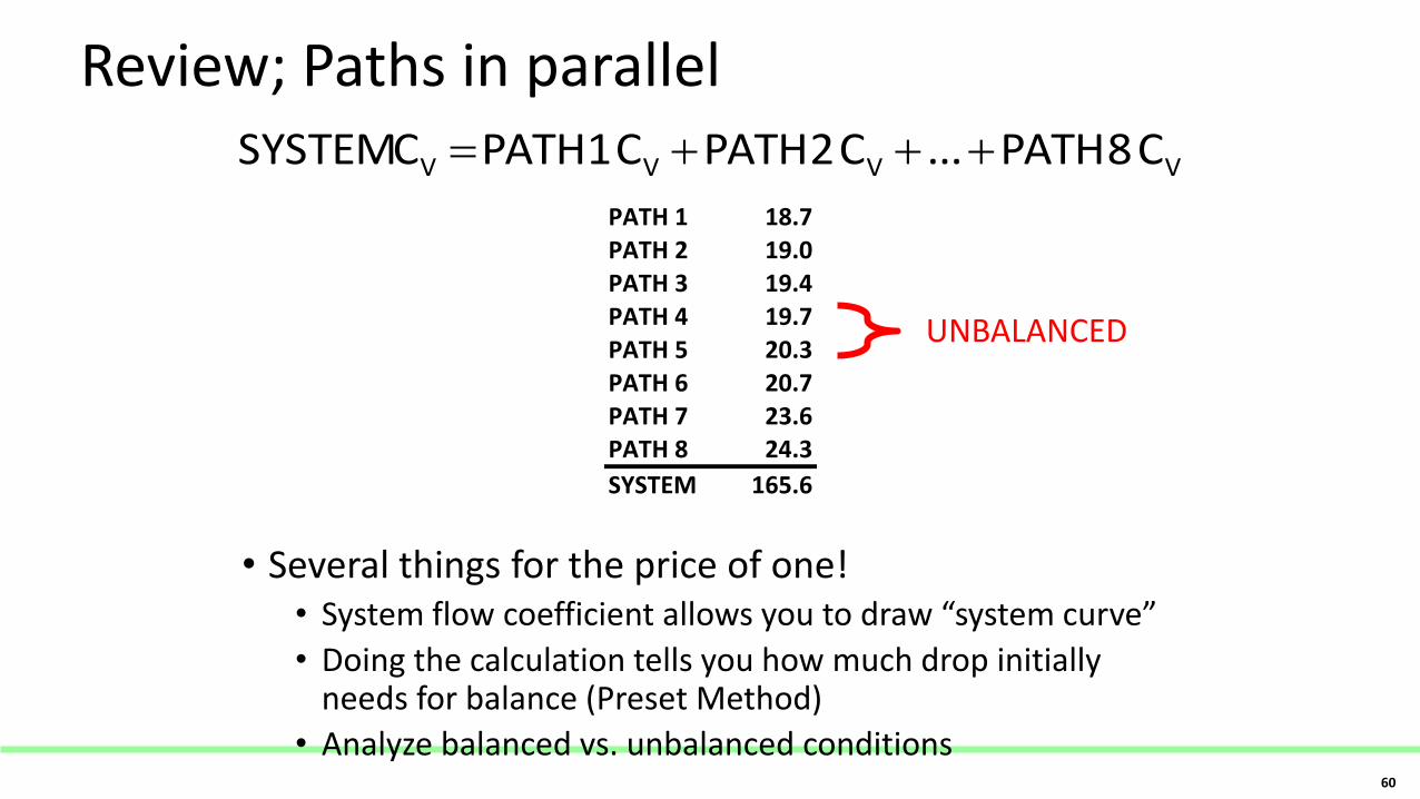
Review; Paths in parallel
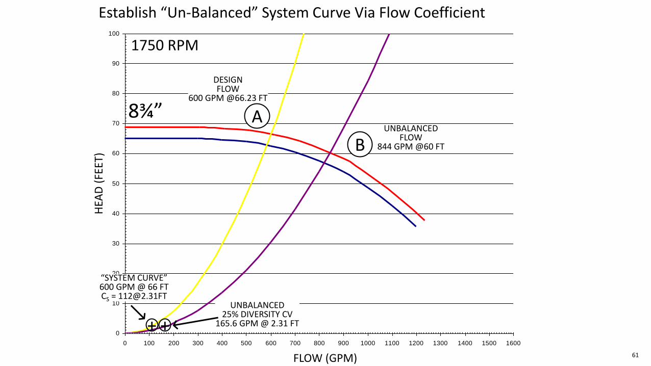
• Several things for the price of one! • System flow coefficient allows you to draw “system curve”
• Doing the calculation tells you how much drop initially needs for balance (Preset Method)
• Analyze balanced vs. unbalanced conditions
VVVV C 8 PATH...C 2 PATHC 1 PATH C SYSTEM
PATH 1 18.7PATH 2 19.0PATH 3 19.4PATH 4 19.7PATH 5 20.3PATH 6 20.7PATH 7 23.6PATH 8 24.3
SYSTEM 165.6
UNBALANCED
60
0
10
20
30
40
50
60
70
80
90
100
0 100 200 300 400 500 600 700 800 900 1000 1100 1200 1300 1400 1500 1600
DESIGN FLOW
600 GPM @66.23 FT
8¾” A
B UNBALANCED
FLOW 844 GPM @60 FT
UNBALANCED 25% DIVERSITY CV
165.6 GPM @ 2.31 FT + +
“SYSTEM CURVE” 600 GPM @ 66 FT CS = [email protected]
FLOW (GPM)
HEA
D (
FEET
)
1750 RPM
Establish “Un-Balanced” System Curve Via Flow Coefficient
61
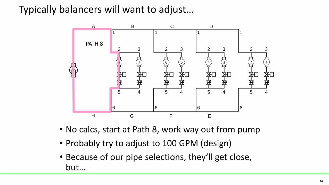
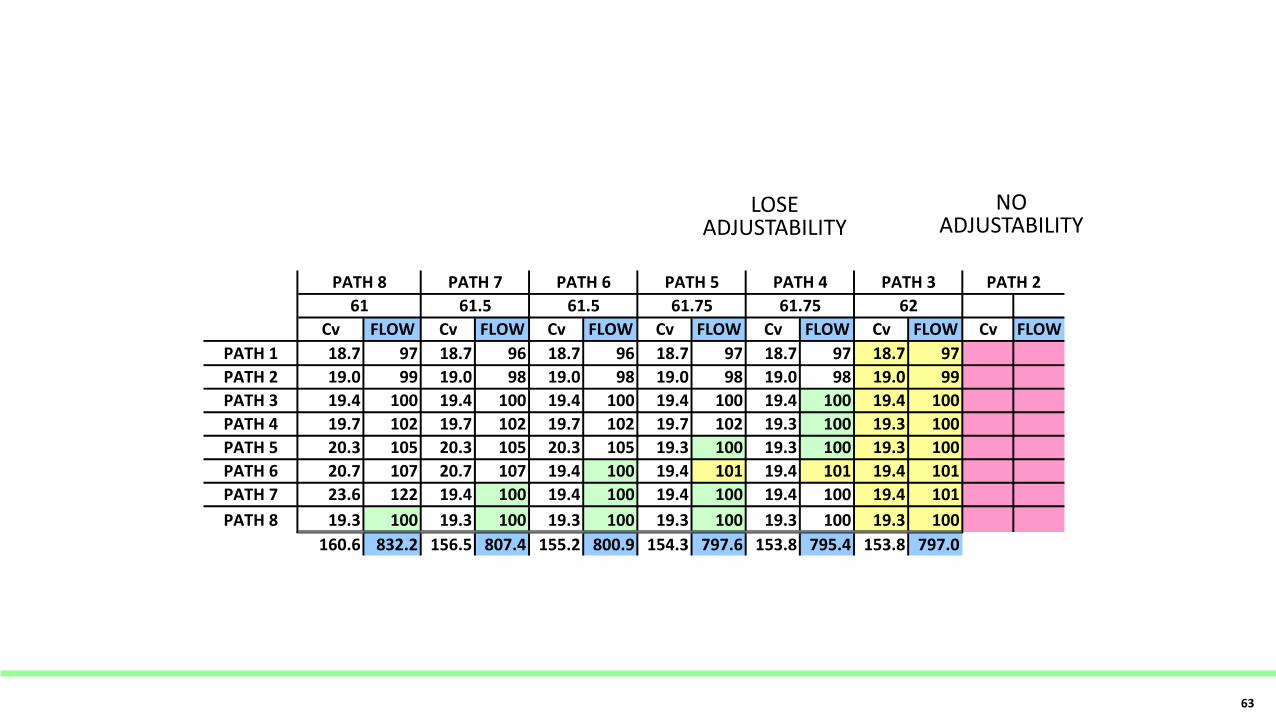
Typically balancers will want to adjust…
• No calcs, start at Path 8, work way out from pump
• Probably try to adjust to 100 GPM (design)
• Because of our pipe selections, they’ll get close, but…
62
A B C D
1
2 3
5 4
6
1
2 3
5 4
6
1
2 3
5 4
6
1
2 3
5 4
6
G F E
1 2 3 4 5 6 7 8
H
PATH 8
Cv FLOW Cv FLOW Cv FLOW Cv FLOW Cv FLOW Cv FLOW Cv FLOW
PATH 1 18.7 97 18.7 96 18.7 96 18.7 97 18.7 97 18.7 97
PATH 2 19.0 99 19.0 98 19.0 98 19.0 98 19.0 98 19.0 99
PATH 3 19.4 100 19.4 100 19.4 100 19.4 100 19.4 100 19.4 100
PATH 4 19.7 102 19.7 102 19.7 102 19.7 102 19.3 100 19.3 100
PATH 5 20.3 105 20.3 105 20.3 105 19.3 100 19.3 100 19.3 100
PATH 6 20.7 107 20.7 107 19.4 100 19.4 101 19.4 101 19.4 101
PATH 7 23.6 122 19.4 100 19.4 100 19.4 100 19.4 100 19.4 101
PATH 8 19.3 100 19.3 100 19.3 100 19.3 100 19.3 100 19.3 100
160.6 832.2 156.5 807.4 155.2 800.9 154.3 797.6 153.8 795.4 153.8 797.0
PATH 2
61.75 62
PATH 8 PATH 7 PATH 6 PATH 5 PATH 4 PATH 3
61 61.5 61.5 61.75
LOSE ADJUSTABILITY
NO ADJUSTABILITY
63
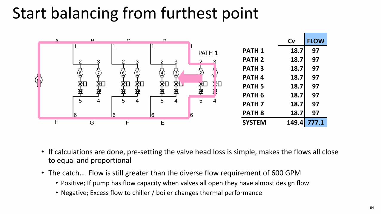
Start balancing from furthest point
• If calculations are done, pre-setting the valve head loss is simple, makes the flows all close to equal and proportional
• The catch… Flow is still greater than the diverse flow requirement of 600 GPM • Positive; If pump has flow capacity when valves all open they have almost design flow
• Negative; Excess flow to chiller / boiler changes thermal performance
Cv FLOW
PATH 1 18.7 97PATH 2 18.7 97PATH 3 18.7 97PATH 4 18.7 97PATH 5 18.7 97PATH 6 18.7 97PATH 7 18.7 97PATH 8 18.7 97
SYSTEM 149.4 777.1
64
A B C D 1
2 3
5 4
6
1
2 3
5 4
6
1
2 3
5 4
6
1
2 3
5 4
6
G F E
1 2 3 4 5 6 7 8
H
PATH 1
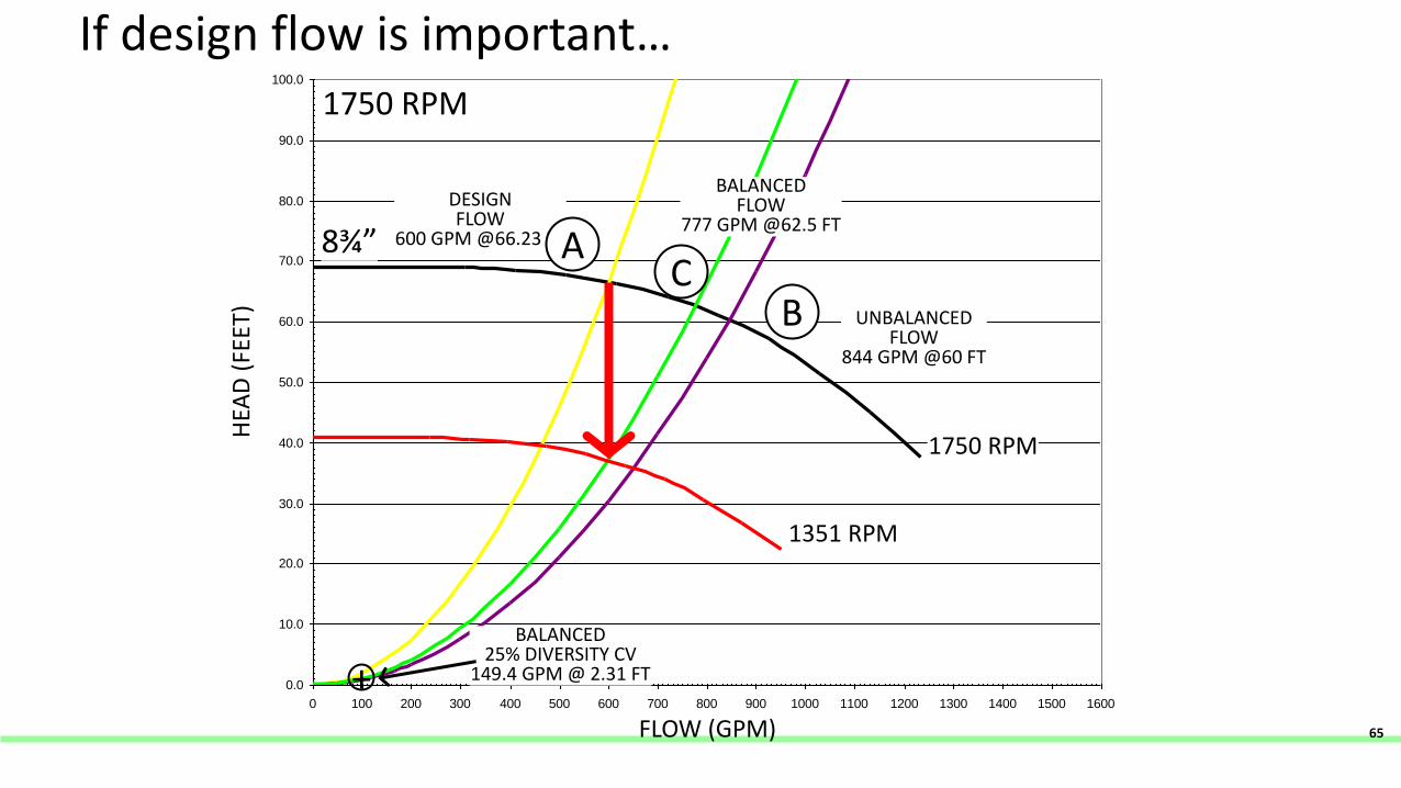
If design flow is important…
0.0
10.0
20.0
30.0
40.0
50.0
60.0
70.0
80.0
90.0
100.0
0 100 200 300 400 500 600 700 800 900 1000 1100 1200 1300 1400 1500 1600
DESIGN FLOW
600 GPM @66.23 FT 8¾” A
B UNBALANCED FLOW
844 GPM @60 FT
BALANCED 25% DIVERSITY CV
149.4 GPM @ 2.31 FT + FLOW (GPM)
HEA
D (
FEET
)
1750 RPM
C
BALANCED FLOW
777 GPM @62.5 FT
1351 RPM
1750 RPM
65
A note on the numbers… • Basic design principles…
• Pump selection just happened to cover unbalanced and balanced flow rates… this doesn’t always happen!
• Not a lot of change in pump head… • Design 66’
• Unbalanced 60’
• Big change in flow because of piping network
• Horsepower • Design: 600 @ 66’/73% → 13.8 Hp
• Unbalanced: 844 @ 60’/81% → 15.8 Hp
• Balanced System All Open: 777 @ 62.5’/80% → 15.3 Hp
• Balanced System Diverse Flow: 600 @ 37.3’/80% → 7 Hp
66
Key to the diverse balance
• Do not primarily adjust Individual paths to the percentage of the diverse flow… • Must adjust to coil full design flow; Coil controller must have ability to get full flow
for design heat transfer
• A diverse pump selection is a “fake” selection point, not necessarily accounting for full design flow
• The “extra” flow paths, or path capacity due to the control valve opening fully will move the system curve out on the pump curve, causing more flow
• How can systems be made to operate better, especially in variable speed • Decision analysis, More involved control algorithms/sequences
67
Control & Balancing Valve
• Standard Modulating Control Valves
• Remember to account for control valve authority effects
• Static Balance Valve provides proportionality and coordinated flow limiting, however VS Pump control area can cause issues
• Flow limiting valves do little to help in this application; Not Proportional
• Under true “design” operation the pump doesn’t have enough capacity
• Far circuits starve (proportionality)
• Pressure Independent Control Valves
• Can limit maximum flow with “start up sequence” from the controller
• Much more integrated control system sequence of operation…don’t expect your balancer or control programmer to figure it out for you
68
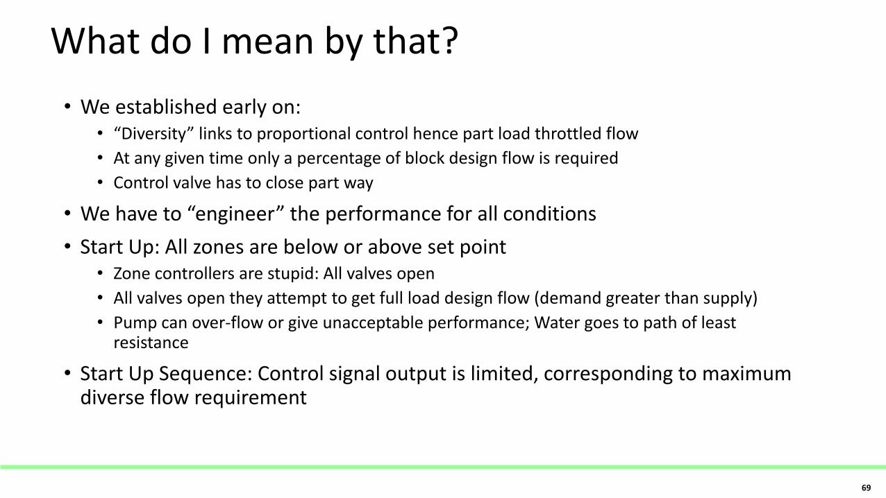
What do I mean by that?
• We established early on: • “Diversity” links to proportional control hence part load throttled flow
• At any given time only a percentage of block design flow is required
• Control valve has to close part way
• We have to “engineer” the performance for all conditions
• Start Up: All zones are below or above set point • Zone controllers are stupid: All valves open
• All valves open they attempt to get full load design flow (demand greater than supply)
• Pump can over-flow or give unacceptable performance; Water goes to path of least resistance
• Start Up Sequence: Control signal output is limited, corresponding to maximum diverse flow requirement
69
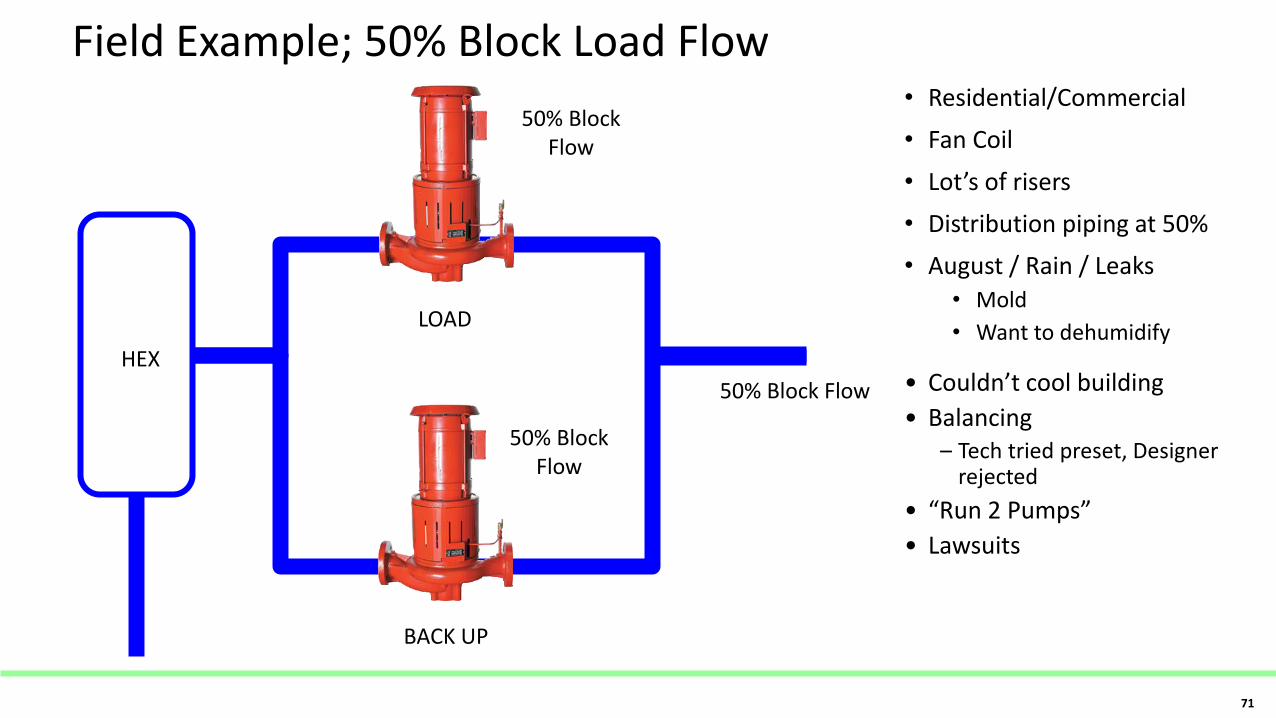
Field Example; 50% Block Load Flow • Residential/Commercial
• Fan Coil
• Lot’s of risers
• Distribution piping at 50%
• August / Rain / Leaks • Mold
• Want to dehumidify
• Couldn’t cool building
• Balancing – Tech tried preset, Designer
rejected
• “Run 2 Pumps”
• Lawsuits
71
HEX
BACK UP
LOAD
50% Block Flow
50% Block Flow
50% Block Flow
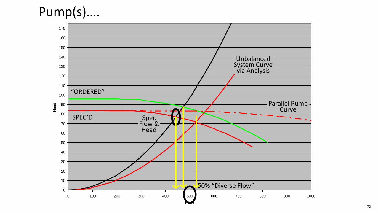
Pump(s)….
0
10
20
30
40
50
60
70
80
90
100
110
120
130
140
150
160
170
0 100 200 300 400 500 600 700 800 900 1000
Flow
Head
SPEC’D
“ORDERED”
50% “Diverse Flow”
Spec Flow & Head
Parallel Pump Curve
Unbalanced System Curve via Analysis
72
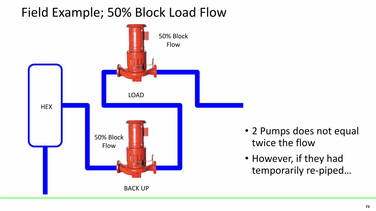
Field Example; 50% Block Load Flow
• 2 Pumps does not equal twice the flow
• However, if they had temporarily re-piped…
73
HEX
BACK UP
LOAD
50% Block Flow
50% Block Flow
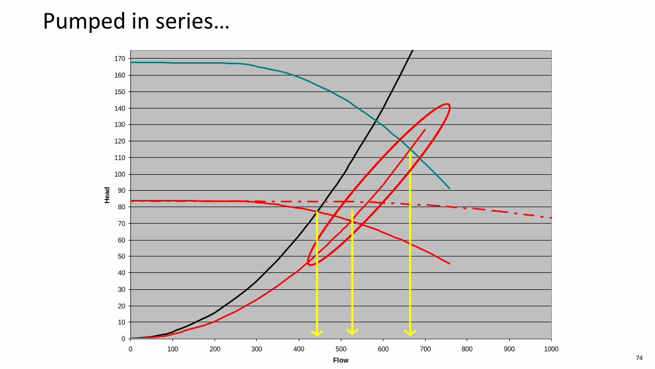
Pumped in series…
74
0
10
20
30
40
50
60
70
80
90
100
110
120
130
140
150
160
170
0 100 200 300 400 500 600 700 800 900 1000
Flow
Head
Is this an uncommon occurrence?
• Probably not • 3 semi-similar occurrences that same year
• What should solution have been? • Re-size certain pipes (Didn’t do)
• Modified distribution system design (more major)
• Modify pumps (Did do)
• Questionable design decisions • Aside from the obvious…
• Fan Coil & 2 Position Valve…
75
Another example… sort of second hand
• PICV Valve application
• Water hammer on floors during commissioning & balancing process
• According to owner… • Valves set at factory for twice as much flow as design schedules
• Think though about similarities • Valve capacity twice that of pump capability to provide… sort of in the same
realm as “diversity”
76
Working Example
• Four Floors
• 2 coils per floor
• 100 GPM per coil
• Direct Return distribution
• 75%/25% Diversity; 800 GPM Block, 600 GPM Design Flow
• Distribution selected at 600 GPM
• Proportional operation and balance
• Required Control Characteristic; Linear • VAV AHU with Outdoor Air Intake
77