Copyright 2001, Society of Petroleum Engineers Inc.

This paper was prepared for presentation at the 2001 SPE Annual Technical Conference andExhibition, 30 September-3 October in New Orleans.

This paper was selected for presentation by an SPE Program Committee following review ofinformation contained in an abstract submitted by the author(s). Contents of the paper, aspresented, have not been reviewed by the Society of Petroleum Engineers and are subject tocorrection by the author(s). The material, as presented, does not necessarily reflect anyposition of the Society of Petroleum Engineers, its officers, or members. Papers presented atSPE meetings are subject to publication review by Editorial Committees of the Society ofPetroleum Engineers. Electronic reproduction, distribution, or storage of any part of this paperfor commercial purposes without the written consent of the Society of Petroleum Engineers isprohibited. Permission to reproduce in print is restricted to an abstract of not more than 300words; illustrations may not be copied. The abstract must contain conspicuousacknowledgment of where and by whom the paper was presented. Write Librarian, SPE, P.O.Box 833836, Richardson, TX 75083-3836, U.S.A., fax 01-972-952-9435.

AbstractOften time when a production engineer conducts a nodalanalysis, he assumes a constant reservoir condition. Typically,a downhole shut-in static pressure will be taken as thereservoir pressure. In this work, we will demonstrate theimportance of using reservoir simulation to model reservoirdynamics in conjunction with other production engineeringtools.

The integration has helped us identify the cause for anextremely high skin generated from a short-term waterinjectivity test. Without reservoir modeling, we cannot besure if the skin was from fine-particle plugging, or clayexpansion, or wellbore debris accumulation. Interestingly, thebuild-up pressure derivatives were quite different prior to andafter 1991. This discrepancy was explained by a partialblockage of one sand layer that was generated by an invadingcement mixture during fire fighting after the Gulf war.

Another example shows use of production logging tosolve a puzzle for a reservoir engineer. There is a vertical welland an expanding secondary gas cap has surrounded its upperportion. Its GOR value has been surprisingly low. Thefindings from production logging also help us characterize thegeology around this well.

Using real examples, we show how to build synergybetween reservoir engineers and production engineers. Thiswork demonstrates the usefulness of reservoir simulation tohelp production engineers diagnose well operation problems.

IntroductionIn a typical operating company, the job responsibilities of areservoir engineer and a production engineer are clearly

defined. They are solving their problems on their own. Evenwhen there are communicating opportunities, mutual trustdoes not exist. For example, a production engineer mayconsider that a recommended production allowable by areservoir engineer is too restrictive or calculated with wronginput data not compatible with field conditions. On the otherhand, a reservoir engineer often complains that the productionengineer is narrowly focused at single well performance anddoes not understand the global reservoir picture.

It is a challenge to bring production and reservoirengineers together to help each other solve field-operatingproblems and develop the full production potential of a field.This paper provides a few examples as to initiate a discussionhow to generate synergy between reservoir and productionengineers.

Field Example 1: Well X-14X-14 is an active producer in Wara formation1 of the GreaterBurgan oil field. It was completed in 1955. Lots of data areavailable including core permeability and porosity, build-uptests over different times, GOR flow tests, etc. Vast amount ofinteresting data over 56 years makes this well an idealcandidate to be studied by reservoir engineers and productionengineers together.

Fault IdentificationFrom a semi-log plot of a build-up test in 1978 as shown inFig. 1, a sealing fault signature can be observed by twostraight lines. Second line’s slope, m2, is exactly double ofthe first line’s slope, m1. The occurrence of single sealingfault effect began about 20 hours after shut-in, which isequivalent to a distance of 496 meters according to the

following equation.

The drawdown period prior to shut-in lasted about 288hours, which was much longer than 20 hours, the timerequired for the pressure wave to reach to the fault. Thisensured the detection of the faults2. If the drawdown time isless than 40 hours, we may not be able to detect the fault in thebuild-up data. Several other build-up tests on this well did not

SPE 71590

Field Examples to Bridge the Gap Between Production Engineering and ReservoirEngineeringH-J. Su, SPE, Chevron Overseas Petroleum Technology Co. and S. Al-Rasheedi, SPE, Kuwait Oil Company

)1.....(..................................................,.........4

029.0φµc

tkr

∆=

2 HO-JEEN SU, SALEH AL-RASHEEDI SPE 71590

have enough drawdown time and the fault signature did notappear on their semi-log plots.

In an effort to reduce production loss, often the shut-intime of a buildup test was designed to be short. As a result,major geological features became not detectable by transientpressure analysis. To look deep at the lost-productionconcern, we found that the lost production from a prolongbuildup test could be made up shortly after the test byproducing at a higher rate temporarily due to a higherreservoir pressure in most cases. Therefore, we recommendan at least 72- hour shut-in time for Wara formation. Itsaverage net pay permeability is about 500md.

A typical production engineer analyzes build-up data toestimate skin and well productivity index. Often he does notcare much about the existence of faults and not try to calculatethe distance of a fault. On the other hand, the fault existenceis a very important piece of information for a reservoirengineer in the case of designing a pattern waterflood. All thewells in a particular pattern have to be located in the same sideof a fault. Definitely, a production engineer needs to be awareof what is going on in the mind of a reservoir engineer andpass vital information to his reservoir-engineering counterpart.

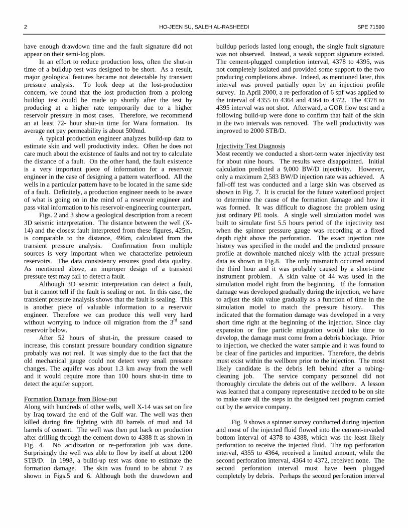
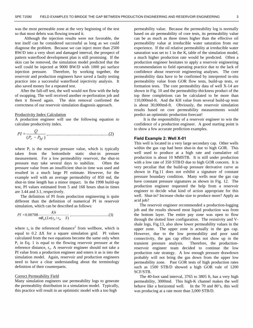
Figs. 2 and 3 show a geological description from a recent3D seismic interpretation. The distance between the well (X-14) and the closest fault interpreted from these figures, 425m,is comparable to the distance, 496m, calculated from thetransient pressure analysis. Confirmation from multiplesources is very important when we characterize petroleumreservoirs. The data consistency ensures good data quality.As mentioned above, an improper design of a transientpressure test may fail to detect a fault.

Although 3D seismic interpretation can detect a fault,but it cannot tell if the fault is sealing or not. In this case, thetransient pressure analysis shows that the fault is sealing. Thisis another piece of valuable information to a reservoirengineer. Therefore we can produce this well very hardwithout worrying to induce oil migration from the 3rd sandreservoir below.

After 52 hours of shut-in, the pressure ceased toincrease, this constant pressure boundary condition signatureprobably was not real. It was simply due to the fact that theold mechanical gauge could not detect very small pressurechanges. The aquifer was about 1.3 km away from the welland it would require more than 100 hours shut-in time todetect the aquifer support.

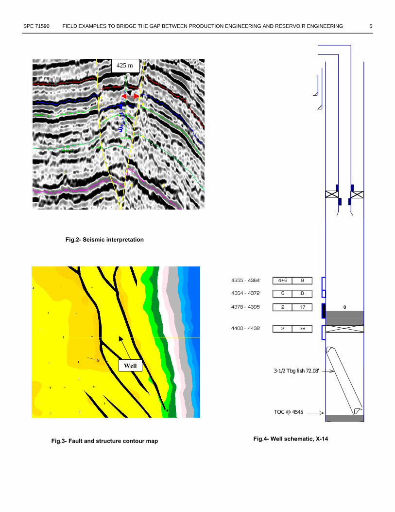
Formation Damage from Blow-outAlong with hundreds of other wells, well X-14 was set on fireby Iraq toward the end of the Gulf war. The well was thenkilled during fire fighting with 80 barrels of mud and 14barrels of cement. The well was then put back on productionafter drilling through the cement down to 4388 ft as shown inFig. 4. No acidization or re-perforation job was done.Surprisingly the well was able to flow by itself at about 1200STB/D. In 1998, a build-up test was done to estimate theformation damage. The skin was found to be about 7 asshown in Figs.5 and 6. Although both the drawdown and

buildup periods lasted long enough, the single fault signaturewas not observed. Instead, a weak support signature existed.The cement-plugged completion interval, 4378 to 4395, wasnot completely isolated and provided some support to the twoproducing completions above. Indeed, as mentioned later, thisinterval was proved partially open by an injection profilesurvey. In April 2000, a re-perforation of 6 spf was applied tothe interval of 4355 to 4364 and 4364 to 4372. The 4378 to4395 interval was not shot. Afterward, a GOR flow test and afollowing build-up were done to confirm that half of the skinin the two intervals was removed. The well productivity wasimproved to 2000 STB/D.

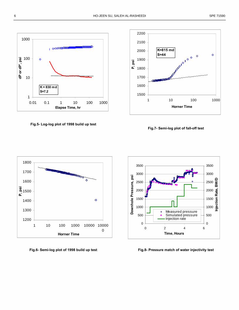
Injectivity Test DiagnosisMost recently we conducted a short-term water injectivity testfor about nine hours. The results were disappointed. Initialcalculation predicted a 9,000 BW/D injectivity. However,only a maximum 2,583 BW/D injection rate was achieved. Afall-off test was conducted and a large skin was observed asshown in Fig. 7. It is crucial for the future waterflood projectto determine the cause of the formation damage and how itwas formed. It was difficult to diagnose the problem usingjust ordinary PE tools. A single well simulation model wasbuilt to simulate first 5.5 hours period of the injectivity testwhen the spinner pressure gauge was recording at a fixeddepth right above the perforation. The exact injection ratehistory was specified in the model and the predicted pressureprofile at downhole matched nicely with the actual pressuredata as shown in Fig.8. The only mismatch occurred aroundthe third hour and it was probably caused by a short-timeinstrument problem. A skin value of 44 was used in thesimulation model right from the beginning. If the formationdamage was developed gradually during the injection, we haveto adjust the skin value gradually as a function of time in thesimulation model to match the pressure history. Thisindicated that the formation damage was developed in a veryshort time right at the beginning of the injection. Since clayexpansion or fine particle migration would take time todevelop, the damage must come from a debris blockage. Priorto injection, we checked the water sample and it was found tobe clear of fine particles and impurities. Therefore, the debrismust exist within the wellbore prior to the injection. The mostlikely candidate is the debris left behind after a tubing-cleaning job. The service company personnel did notthoroughly circulate the debris out of the wellbore. A lessonwas learned that a company representative needed to be on siteto make sure all the steps in the designed test program carriedout by the service company.

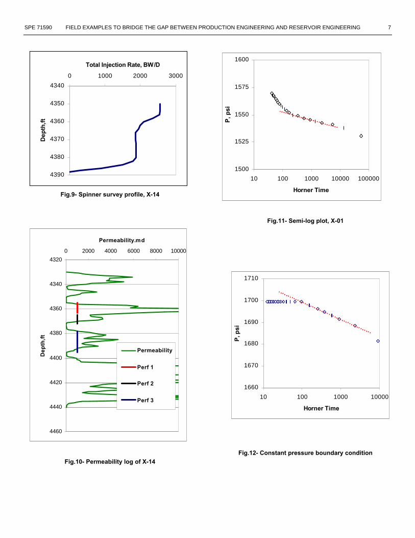
Fig. 9 shows a spinner survey conducted during injectionand most of the injected fluid flowed into the cement-invadedbottom interval of 4378 to 4388, which was the least likelyperforation to receive the injected fluid. The top perforationinterval, 4355 to 4364, received a limited amount, while thesecond perforation interval, 4364 to 4372, received none. Thesecond perforation interval must have been pluggedcompletely by debris. Perhaps the second perforation interval

SPE 71590 FIELD EXAMPLES TO BRIDGE THE GAP BETWEEN PRODUCTION ENGINEERING AND RESERVOIR ENGINEERING 3

was the most permeable zone at the very beginning of the testso that most debris was flowing toward it.

Although the injection results were not favorable, thetest itself can be considered successful as long as we coulddiagnose the problem. Because we can inject more than 2500BW/D into a very short and damaged interval, the prospect ofpattern waterflood development plan is still promising. If theskin can be removed, the simulation model predicted that thewell could be injected at 9000 BW/D with 1000 psi surfaceinjection pressure. Therefore, by working together, thereservoir and production engineers have saved a faulty testingpractice into a successful waterflood injectivity analysis. Italso saved money for a repeated test.

After the fall-off test, the well would not flow with the helpof swapping. The well received another re-perforation job andthen it flowed again. The skin removal confirmed thecorrectness of our reservoir simulation diagnosis approach.

Productivity Index CalculationA production engineer will use the following equation tocalculate productivity index.

where Pr is the reservoir pressure value, which is typicallytaken from the bottomhole static shut-in pressuremeasurement. For a low permeability reservoir, the shut-inpressure may take several days to stabilize. Often thepressure value from an insufficient shut-in time was used andresulted in a much large PI estimate. However, for theexample well with an average permeability of 850 md, theshut-in time length has a minor impact. In the 1998 build-uptest, PI values estimated from 5 and 168 hours shut-in timesare 3.44 and 3.1, respectively.

The definition of PI from production engineering is quitedifferent than the definition of numerical PI in reservoirsimulation, which can be described as follows:

where ro is the referenced distance2 from wellbore, which isequal to 0.2 ∆X for a square simulation grid. PI valuescalculated from the two equations become the same only whenPr in Eq. 1 is equal to the flowing reservoir pressure at thereference distance, ro. A reservoir engineer should not take aPI value from a production engineer and enters it as is into thesimulation model. Again, reservoir and production engineersneed to have a clear understanding about the terminologydefinition of their counterparts.

Correct Permeability FieldMany simulation engineers use permeability logs to generatethe permeability distribution in a simulation model. Typically,this practice will result in an optimistic model with a too high

permeability value. Because the permeability log is normallybased on air permeability of core tests, its permeability valuecan be as much as three times higher than the effective oilpermeability value at irreducible water saturation from ourexperience. If the oil relative permeability at irreducible watersaturation was set to 1 in the Kr table of the simulation model,a much higher production rate would be predicted. Often aproduction engineer hesitates to apply a reservoir engineeringrecommendation to field operating practice due to the lack ofconfidence about reservoir engineering analyses. The corepermeability data have to be confirmed by interpreted in-situpermeability value from GOR flow tests, build-up tests, orformation tests. The core permeability data of well X-14 areshown in Fig. 10 and the permeability-thickness product of thetop three completions can be calculated to be more than110,000md-ft. And the KH value from several build-up testsis about 30,000md-ft. Obviously, the reservoir simulationresults based on core permeability measurements wouldpredict an optimistic production forecast!

It is the responsibility of a reservoir engineer to win theconfidence of a production engineer. A good starting point isto show a few accurate prediction examples.

Field Example 2: Well X-01This well is located in a very large secondary cap. Other wellswithin the gas cap had been shut-in due to high GOR. Thiswell used to produce at a high rate and cumulative oilproduction is about 10 MMSTB. It is still under productionwith a low rate of 350 STB/D due to high GOR concern. It isvery peculiar that the build-up pressure derivative curve asshown in Fig.11 does not exhibit a signature of constantpressure boundary condition. Many wells near the gas caphave constant pressure signatures as shown in Fig. 12. Theproduction engineer requested the help from a reservoirengineer to decide what kind of action appropriate for thiswell. Shut-in? Increase choke size to produce more? Apply anacid job?

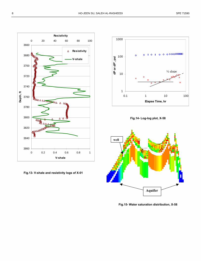
The reservoir engineer recommended a production-loggingjob and the results showed most liquid production was fromthe bottom layer. The entire pay zone was open to flowthrough the slotted liner configuration. The resistivity and V-shale logs, Fig.13, also show lower permeability values in theupper zone. The upper zone is actually in the gas cap.However, due to the low permeability and poor sandconnectivity, the gas cap effect does not show up in thetransient pressure analysis. Therefore, the production-reservoir engineer team decided to continue the lowproduction rate strategy. A low enough pressure drawdownprobably will not bring the gas down from the upper lowpermeability zone. Past GOR tests of high production ratessuch as 1500 STB/D showed a high GOR vale of 1200SCF/STB.

The 40-foot sand interval, 3765 to 3805 ft, has a very highpermeability, 3000md. This high-K channel makes the wellbehave like a horizontal well. In the 70 and 80’s, this wellwas producing at a rate more than 3,000 STB/D.

)2......(........................................,.........)( bfr PP

QPI

−=

)3.........(....................,.........)/((

00708.0SrrLnB

KhPI

woo +=

µ

4 HO-JEEN SU, SALEH AL-RASHEEDI SPE 71590

Field Example 3: Well X-58This well is located in a high-permeability channel as shownby the half slope line in Fig. 14. Openhole logs also show athin sand bedding. The constant pressure boundary conditionis observed after the linear flow period. Since the well is faraway from the gas cap, the reservoir-production engineeringteam decided that the support must come from the aquifer.The distance between the well and the aquifer was interpretedfrom Eq. 1 to be 1500m, which was also consistent to thegeological model and original W/O contact data. Fig. 15shows a cross-section view of water saturation distributionaround the well. Modern graphics software package to displayreservoir simulation results is easy to use and can be a greattool to a production engineer for understanding reservoirdynamics and solving day to day operation problems.

The reservoir engineer was very excited about theinformation of aquifer strength. Since there were very fewwells drilled in the north flank area and none of existingproducers has reported water production, the reservoirengineer had difficulty to specify aquifer strength in thesimulation model. Without the knowledge about the aquiferstrength, it is impossible to design a field development plan orpredict future production. In fact, this buildup test was donemore than 15 years ago, but the information has not beenshared to the reservoir engineer until recently. Therefore, theinformation sharing has to be done in a timely manner.

Conclusions1. We have demonstrated the usefulness of reservoir

simulation in a water injectivity test problem. Workingwith a reservoir engineer, a production engineer cananalyze test results thoroughly and identify causes of poorinjectivity. It also eliminates the need of repeating a test.

2. Sometimes, contradictory transient pressure data for agiven well over different times require the help from botha production engineer and a reservoir engineer tounderstand the event occurred in the well history.Consequently, proper actions can be taken to remove theadverse effect on the reservoir performance by a pastevent.

3. Both a reservoir engineer and a production engineershould have a good understanding of each other’s job. Bealert to any piece of information valuable to the other andpass that information in a timely manner. The operatingunit will be greatly benefited from the synergy ofproduction engineering and reservoir engineering.

4. A reservoir engineer should integrate production datasuch as transient pressure test data into the simulationmodel building process.

5. When a production engineer makes decision about awork-over job, it is very helpful to consult with areservoir engineer regarding aquifer support, gas capexpansion, sand continuity, and over-all field pressure

decline, etc. Understanding total reservoir picture leads toa better solution for a field operation problem.

Nomenclaturec = total compressibility, 1/psih = sand thickness, ftk = permeability, mdkr = relative permeability, fractionP = pressure, psiPr = reservoir pressure, psiPbf = bottom hole flowing pressure, psiq = flow rate, STB/Dro = reference radius for numerical PI, ftr = radial distance, fttp = producing time, hr∆t = shut-in time, hrµ = viscosity, cpφ = porosity, fraction

AcknowledgmentWe are indebted to the management of Kuwait Oil Companyfor permission to publish this work. Support of Chevronmanagement is also appreciated. We would like to thank JohnFalck and Jess Brookly of Chevron for their design of waterinjectivity test and Joon Kim of Chevron for the work ofseismic interpretation. Discussions from Vegesna Raju andWael Al-Qahss of KOC are very helpful.

References1. Moon, M. S., Pederson, J. M., Osman, K., Al-Saied, M., Al-

Sabea, S., and Al-Shammari, H.: “Application ofPetrophysically Derived “Flow Facies” for ReservoirCharacterization and Simulation: Wara Reservoir, GreaterBurgan Field,” paper SPE 49217 presented at the 1998 SPEAnnual Technical Conference and Exhibition, New Orleans,LA, 27-30 September.

2. Earlougher, Robert C. Jr.: “Practicalities of Detecting FaultsFrom Buildup Testing,” paper SPE 8781, JPT 1980.

3. Peaceman, D.W.:“Interpretation of Well-Block Pressure inNumerical Reservoir Simulation with Non Square Grid Blocksand Anisotropic Permeability” SPEJ (June, 1983).

Fig.1- Semi-log plot

1760

1780

1800

1820

0.01 0.1 1 10 100

Delta t, hours

Pre

ss

ure

, ps

i

m1

m2

SPE 71590 FIELD EXAMPLES TO BRIDGE THE GAP BETWEEN PRODUCTION ENGINEERING AND RESERVOIR ENGINEERING 5

Fig.2- Seismic interpretation

Fig.3- Fault and structure contour map Fig.4- Well schematic, X-14

4355 - 4364' 4+6 9

4364 - 4372' 6 8

4378 - 4395' 2 17 0

4400 - 4438' 2 38

3-1/2 Tbg fish 72.08'

TOC @ 4545

425 m

Well

6 HO-JEEN SU, SALEH AL-RASHEEDI SPE 71590

Fig.5- Log-log plot of 1998 build up test

Fig.6- Semi-log plot of 1998 build up test

Fig.7- Semi-log plot of fall-off test

Fig.8- Pressure match of water injectivity test

0

500

1000

1500

2000

2500

3000

3500

0 2 4 6

Time, Hours

Dow

nh

ole

Pre

ssu

re, p

si

0

500

1000

1500

2000

2500

3000

3500

Inje

ctio

n R

ate,

BW

/DMeasured pressureSimulated pressureInjection rate

1

10

100

1000

0.01 0.1 1 10 100 1000Elapse Time, hr

dP

or

dP

', p

si

K = 830 mdS=7.2

1200

1300

1400

1500

1600

1700

1800

1 10 100 1000 10000 100000

Horner Time

P, p

si

1500

1600

1700

1800

1900

2000

2100

2200

1 10 100 1000

Horner Time

P, p

si

K=815 mdS=44

SPE 71590 FIELD EXAMPLES TO BRIDGE THE GAP BETWEEN PRODUCTION ENGINEERING AND RESERVOIR ENGINEERING 7

Fig.9- Spinner survey profile, X-14

Fig.10- Permeability log of X-14

1500

1525

1550

1575

1600

10 100 1000 10000 100000

Horner Time

P, p

siFig.11- Semi-log plot, X-01

Fig.12- Constant pressure boundary condition

4340

4350

4360

4370

4380

4390

0 1000 2000 3000

Total Injection Rate, BW/D

Dep

th,f

t

1660

1670

1680

1690

1700

1710

10 100 1000 10000

Horner Time

P, p

si

4320

4340

4360

4380

4400

4420

4440

4460

0 2000 4000 6000 8000 10000

Permeability.md

Dep

th,f

t

Permeability

Perf 1

Perf 2

Perf 3

8 HO-JEEN SU, SALEH AL-RASHEEDI SPE 71590

Fig.13- V-shale and resistivity logs of X-01

Fig.14- Log-log plot, X-58

Fig.15- Water saturation distribution, X-58

3660

3680

3700

3720

3740

3760

3780

3800

3820

3840

3860

0 20 40 60 80 100

Resistivity

De

pth

, ft

0 0.2 0.4 0.6 0.8 1

V-shale

Resistivity

V-shale

1

10

100

1000

0.1 1 10 100

Elapse Time, hr

dP

or

dP

', p

si

Aquifer

well

½ slope