SPE 167242

Evaluation of Time-Rate Performance of Shale Wells using the Transient Hyperbolic Relation D. S. Fulford, Apache Corporation, T. A. Blasingame, Texas A&M University

Copyright 2013, Society of Petroleum Engineers This paper was prepared for presentation at the SPE Unconventional Resources Conference-Canada held in Calgary, Alberta, Canada, 5–7 November 2013. This paper was selected for presentation by an SPE program committee following review of information contained in an abstract submitted by the author(s). Contents of the paper have not been reviewed by the Society of Petroleum Engineers and are subject to correction by the author(s). The material does not necessarily reflect any position of the Society of Petroleum Engineers, its officers, or members. Electronic reproduction, distribution, or storage of any part of this paper without the written consent of the Society of Petroleum Engineers is prohibited. Permission to reproduce in print is restricted to an abstract of not more than 300 words; illustrations may not be copied. The abstract must contain conspicuous acknowledgment of SPE copyright.

Abstract In this work we present the "Transient Hyperbolic" relation for the analysis and interpretation of time-rate performance data from wells in shale gas/liquids-rich shale plays. This model assumes a transient "b(t)" function which has constant early-time and constant late-time values, with an exponentially decaying transition function. This "b(t)" function is derived from the Gompertz logistic function. Our goal in developing this formulation is to represent the early-time (or clean-up) portion of the production profile (often a hyperbolic function), the transition to the terminal hyperbolic behavior, and finally, the terminal hyperbolic behavior — where the terminal hyperbolic is usually representative of the "non-interfering" vertical fractures in a multi-fractured horizontal well (MFHW). We could further modify this relation to have a terminal exponential decline (thought to represent the performance of the stimulated-reservoir-volume (or SRV)), but that is not a primary purpose of this work — our primary purpose is to demonstrate the "Transient Hyperbolic" nature of the flow behavior from a multi-fractured horizontal well in a shale gas/liquids-rich shale play. The technical contributions of this work are:

• Development of the "Transient Hyperbolic" time-rate relation — this relation includes an early AND a late-time hyperbolic behavior, as well as a logistic transition function.

• Application of the “Transient Hyperbolic” time-rate relation to modeling completion heterogeneity in a MFHW by a superposition of divisions that have differing durations of linear flow.

• Application of the "Transient Hyperbolic" time-rate relation to several field cases — specifically: tight gas, shale gas, and "liquids-rich" shale cases.

Introduction The classic Arps [1945] decline curve approach is limited to cases where wells are producing in boundary dominated-flow (implying a b-parameter between 0 and 1.0) and the b-parameter can be described by a constant value. In practice, we observe values of the b-parameter above 1.0 for extended periods of time prior to the onset of boundary-dominated flow. This difference between theory and application leads to the misapplication of the Arps time-rate relation where the b-parameter applied to early-time data is assumed to be greater than 1.0, and held constant until a terminal exponential decline rate is reached (Modified Hyperbolic Model). This approach assumes prior knowledge of both the average b-parameter for the life of the well, and the terminal exponential decline rate; both of which are unknown for many emerging unconventional plays and may differ within a play as a result of well design. Recent attempts to address this issue have resulted in more rigorous models, such as the Power-Law Exponential (Ilk et al [2008]); however, the Modified Hyperbolic Model remains in popular use within the industry. The approach in this paper is to investigate a modification of the Arps hyperbolic model, as an attempt to reconcile the limitations of the original time-rate relation with the long duration transient flow periods observed in shale gas/liquids-rich shale wells. The reasoning for the investigation into a logistic function to represent the Arps’ b-parameter is best understood

2 SPE 167242

by looking at the application of this form of logistic growth function, as applied in other areas of study. Logistic functions find use in modeling complex behaviors such as population growth and product adoption within markets, which share a unique aspect in common – an increase in saturation within a confined space as individual members of a population transition between a binary state. This approach makes sense from a physical interpretation as applicable to the change in b-parameter over time (b(t)) as individual points or areas (both along an individual fracture stage and among all different fracture stages) within a confined reservoir area transition from transient flow to boundary-dominated flow – either those points are infinite-acting, or they “feel” boundaries. This application assumes a constant maximum and minimum b-parameter, which is applicable to tight gas and unconventional reservoirs. Empirical observations and numerical modeling have demonstrated long duration linear flow exhibiting a hyperbolic exponent of 2.0, some period of transition to the terminal hyperbolic exponent, and boundary-dominated flow exhibiting a hyperbolic exponent of < 0.5 (in a single layer, homogeneous reservoir). Any discussion of the Arps hyperbolic relation, and especially one describing a modification, must begin with a definition of the hyperbolic parameters. Arps presented the “loss-ratio” and “derivative of the loss-ratio” as:

dtdq

q

Da

/

1−≡≡ (Definition of the Loss-Ratio) ................................................................. (1)

[ ]

−≡

≡≡

dtdq

q

dt

d

Ddt

dadt

db/

1 (Derivative of the Loss-Ratio) ................................................................. (2)

Where Eq. 1 and Eq. 2 are written in terms of “modern” variables (i.e., q, D, b), and are based on empirical observations. The resulting hyperbolic rate decline relation is given by:

btD

D

i

+=

11

................................................................................................................................................................. (3)

( ) bi

i

tbDqq

11

1

+= ................................................................................................................................................... (4)

Eq. 3 is relevant as it must be derived for the proposed Transient Hyperbolic b-parameter, and will be used to demonstrate fitness of the model. The Transient Hyperbolic Model The Transient Hyperbolic b-parameter is given by:

( ) [ ][ ][ ]γexpexp exp ) ( )( minmaxmax +−−−−−= elfttcbbbtb ............................................................................ (5)

Where:

bmax = Maximum hyperbolic coefficient [constant b-parameter at early-time linear flow regime]

bmin = Minimum hyperbolic coefficient [constant b-parameter at boundary-dominated flow regime]

telf = Time to end of linear flow [beginning of transition from bmax to bmin]

γ = Euler-Mascheroni constant [0.57721566…]

c = Scaling factor [controls the rate of transition of the function from bmax to bmin]

The scaling factor is given by:

[ ]

elftc

5.1

exp γ= .................................................................................................................................................................... (6)

Recalling the definitions of the hyperbolic parameters, we can substitute Eq. 5 into Eq. 2, perform integration, and take the reciprocal to produce:

SPE 167242 3

( )( ) [ ][ ][ ] [ ][ ][ ][ ]γγ expexp- Eiexpexp- Ei) ( 1

1minmax

max +−+−−−

++=

elfelf

i

tcttcc

bbtbD

tD ........... (7)

Where “Ei” is the exponential integral function. Eq. 7 can be substituted into Eq. 2 and integrated to yield:

( )( ) [ ][ ][ ] [ ][ ][ ][ ]

+−+−−−

++−= ∫ dt

tcttcc

bbtb

D

tqtq

elfelf

i

i

γγ expexp- Eiexpexp- Ei) (

11

0exp

minmaxmax

... (8)

A derivation of these parameters is provided in Appendix A. Type curves illustrating the behavior of these functions are given in Fig. 1 – 8. The behavior of Eq. 5 was suggested by Kupchenko et al [2008] for bounded channel reservoirs where the hydraulic facture spanned the entire length of the reservoir. However, the primary purpose of the work was to investigate tight gas sands, and the example was generated to investigate the effect of long-term linear flow on the b-parameter in 0.01 md reservoirs. The plots of the b-parameter versus time, reproduced in Fig. 7 by the b(t) function, illustrate the asymmetric sigmoid shape characteristic of the Gompertz function, transitioning from b = 2 in linear flow, to b <= 0.5 in boundary-dominated flow, with a transition time between these two regimes. We must note the character of the D-parameter for the Transient Hyperbolic model. Duration each distinct flow regime – that is, in linear flow and in boundary-dominated flow – it will display a straight line trend in the D-parameter on a log-log plot versus time (Fig. 5). This causes both a convex and concave curve, with concavity following convexity. The addition of the D∞ parameter in the Power-Law Exponential is intended to fit this behavior by causing convexity late in time. The terminal decline parameter of the Modified Hyperbolic performs the same function, only at very late time and with a severe treatment. The Transient Hyperbolic model fits this behavior directly. The terminal decline in Eq. 5 is represented by bmin and telf. Wattenbarger et al [1998] described a solution for linear flow in a hydraulically fractured well whose fracture extends to the lateral boundaries, illustrated in Fig 9., and provided an equation to forecast the end of linear flow in these wells, given by:

( ) 2

00633.0

eit

Dye

yc

tktµφ

= ....................................................................................................................................................... (9)

In the constant drawdown scenario, the end of half-slope on a log-log plot of rate versus time was determined to occur at𝑡𝐷𝑦𝑒 = 0.25, from visual inspection of the plot. This value can be substituted into Eq. 9 and re-arranged to yield:

( )( ) ( )

k

yc

k

yct etetehs

02532.000633.0

25.0 22 µφµφ== ..................................................................................................................... (10)

Different methods of estimation of tehs have been suggested (e.g. Nobakht et al [2010]), but an important point of distinction must be made; these methods estimate the time at which half-slope ends on the log-log rate versus time plot. Although sometimes referenced in literature as telf, this value is not actually the time at which the b-parameter begins transition from bmax, but the time at which that transition becomes visible in diagnostic plots of the time-rate data. For the purpose of this paper, tehs refers to Wattenbarger et al’s original definition as the visual identification of deviation from straight-line half-slope, and telf refers to the time at which the b-parameter begins to transition from bmax. The value of bmin has been shown to vary depending on reservoir heterogeneity (Ambrose et al [2011], Nobakht et al [2011]). In general, it is < 0.5 for a single layer, homogeneous reservoir, and > 0.5, demonstrated to be around 0.7 – 0.8, for a heterogeneous reservoir. An increase in reservoir heterogeneity has been shown to lead to an increase in the value of bmin. In order to calibrate Eq. 5 and Eq. 6, a numerical model was developed similar to that shown in Fig. 1 as a single layer with a single hydraulic facture that spans the entire length of the reservoir (ye). The hydraulic fracture has infinite conductivity, and the reservoir is a homogeneous, single phase system with constant permeability. Ten (10) cases were created based on these properties, with varying ye from 25 ft to 250 ft, in 25 ft increments. This represents a fracture spacing of 50 ft to 500 ft. The reservoir properties are shown in Table 1.

4 SPE 167242

Table 1 – Numerical model properties – 10 cases with varying reservoir length (ye) Model Properties

ye 25 to 250 ft ϕ 0.06

Sw 0.30 pi 3,500 psi pwf 300 psi km 0.0001 md h 300 ft xf 500 ft kfw ∞ md-ft

The b-parameter of the numerical cases versus 𝑡𝐷𝑦𝑒 is shown in Fig. 10. The values of 𝑡𝐷𝑦𝑒,𝑒𝑙𝑓 and 𝑡𝐷𝑦𝑒,𝑏𝑑𝑓 are determined as the points at which the b-parameter falls below bmax and reaches bmin, respectively.

1.0, =elfDyet ................................................................................................................................................................ (11)

7.0, =bdfDyet ............................................................................................................................................................... (12)

As all cases exhibit follow this trend, it implies these two values are proportional. We can then write tbdf as a function of telf:

( ) elfelfelf

elfDye

bdfDyeelfbdf ttt

t

ttt 0.7

1.0

7.0 ,

, === ............................................................................................................. (13)

And relate tehs to telf by:

( ) elfelfelf

elfDye

ehsDyeelfehs ttt

t

ttt 5.2

1.0

25.0 ,

, === ........................................................................................................... (14)

Eq. 11 can be substituted into Eq. 9 to yield:

( )( ) ( )

k

yc

k

yct etetelf

0633.000633.0

1.0 22 µφµφ== ......................................................................................................................... (15)

Which is the time at which b(t) begins to transition from bmax. From Fig. 10, it is clear that b(t) is a unique solution for any given set of reservoir parameters, and therefore the scaling factor, c, must be calibrated to allow b(t) to transition from bmax @ telf, to bmin @ tbdf. This implies c must also have a unique solution, which is given by Eq. 6. A full derivation of c is provided in Appendix B. With this calibration performed, the model can be fit to the numerical cases. A fit to each numerical case is given in Fig. 11 – 24. A comparison between the model EUR and the numerical EUR is presented in Fig. 25, and summarized in Table 2. The parameters used in the fit are summarized in Table 3.

SPE 167242 5

Table 2 – EUR (Gp) comparison between Transient Hyperbolic Model and Numerical Cases Reservoir Length, ye

(ft) Numerical EUR

(MMCF) Model EUR

(MMCF) Percent Error

% 25 254 250 -1.7 50 508 508 0.0 75 754 756 0.2 100 980 983 0.4 125 1,177 1,181 0.4 150 1,342 1,346 0.3 175 1,475 1,477 0.1 200 1,579 1,578 -0.1 225 1,656 1,653 -0.2 250 1,714 1,707 -0.4

Table 3 – Transient Hyperbolic Model Parameters for Numerical Cases

qi (MSCF/D)

Di dimensionless

bmax dimensionless

bmin dimensionless

5000 0.282 2.0 0.38

Field Observation of Logistic Behavior of the b-Parameter For verification of the proposed logistic transition of the b-parameter, the model was fit to a Mexico Tight Gas Well. This well has been producing for over 30 years, and has had only minor disruptions in its production history for the duration of its life. Fig. 26 illustrates this fit. The model provides an excellent match for flow rate (q), D-parameter, and b-parameter, as the transition from linear flow to boundary-dominated flow occurs over a period of 22 years. This verification in a homogeneous completion provides a basis for more complex modeling in a MFHW.

Modeling Completion Heterogeneity in a MFHW The logistic transition of the b-parameter allows for modeling of individual fracture stages within a MFHW. Each stage is homogeneous by itself and transitions from a bmax of 2.0 to a bmin of 0.5. Together, they create a superposition of the b-parameter as each fracture stage transitions at a different time and rate. This completion heterogeneity can then, itself, also be represented by some bmax to bmin transition. Fig. 27 illustrates a heterogeneous completion, where divisions 2, 3, 4, 5, 6, and 7 respectively require 4, 9 16, 20.25, 25, and 132.25 times longer to reach telf than the first division. The divisions represent pseudo-fractures that group reservoir volumes transitioning out of linear flow at the same time. Nobakht et al [2011] provided a method to calculate the proportion of flow rate (q) and tehs for each division with the following functions:

jjj qq βα= ................................................................................................................................................................ (16)

Where αj represents the proportion of the reservoir flowing from each reservoir division, and βj represents the ratio of the pseudo-fracture half-length for each division to the maximum fracture half-length.

( )maxfw

jfjj

xL

xd ∑=α ........................................................................................................................................................ (17)

( )

jf

fj

dx

dxmax=β .......................................................................................................................................................... (18)

And:

d = Half of the distance between frac stages

dj = Half of the distance between adjacent fractures in division j

∑ jfx = sum of all fracture half-lengths in division j [both sides of a fracture must be considered]

fx = average fracture half-length [of all fractures, not just division j]

6 SPE 167242

( )maxfx = maximum fracture half-length among all divisions

Lw = length of the horizontal well [assumed to be 2(n)(d), where n is the number of fracture stages]

The time to end of linear flow for each division assumes a homogeneous reservoir, and is given by:

( )2jelfelfj ddtt = ........................................................................................................................................................ (19)

Using Eqs. 16 – 18, and the heterogeneous completion in Fig. 27, we can calculate an initial rate (q) and telf for each division, and use Eq. 5 to model each division as a pseudo-fracture. Each division uses a bmax of 2.0, and a bmin of 0.5. The flow rate for each division was summed to achieve a total well flow rate (“superposition flow rate”), and a Transient Hyperbolic model to represent the entire well was fit to this rate. A plot of the flow rate for all divisions is shown in Fig. 28. A fit for flow rate and cumulative production is shown in Fig. 29. The superposition b-parameter is shown in Fig. 30, and the superposition D-parameter in shown in Fig. 31. The EUR is listed in Table 4.

Table 4 – Transient Hyperbolic Model Fit of a Heterogeneous MFHW well Superposition EUR

BCF Model EUR

BCF 2.47 2.50

The b-parameter required to fit the superposition is b = 0.7. This result agrees with Nobakht et al [2011], given that the model used in Fig. 27 is a recreation and not an exact match. As completion heterogeneity increases, the value of the terminal b-parameter required for a good fit will increase. It is interesting to note that the superposition b-parameter never reaches the bmin = 0.5 that was set as the value for each division during the economic life of the well. This application demonstrates that the logistic transition of the b-parameter is in agreement with empirical observation of b-parameters > 0.5 in heterogeneous completions. The application to MFHWs using a bmin > 0.5 is well founded. Applications to Field Data In this section the Transient Hyperbolic (TH) model is applied to several field cases and compared against the Power-Law Exponential (PLE) and Modified Hyperbolic (MH) models. Several different shale plays in North America are considered here. Field A is a formation composed of siltstone and dark grey shale, with dolomitic siltstone in the base and fine grained sandstone toward the top. It is 400 – 500 ft thick and contains very little clay content. The formation is slightly over pressured with a pressure gradient of 0.50 – 0.65 psi/ft. Field B is a black, organic rich shale of Upper Jurassic age, which is deposited mainly with heavier clay minerals, silica, and calcite. The depth of Field B ranges from approximately 10,000 ft in the northwest to 14,000 ft in the southeast. It is overpressured with pressure gradients higher than 0.9 psi/ft. Field C is a Middle Devonian age black, low density, organic rich shale at an approximate average depth of 5,000 – 6,000 ft. We also present an East Texas Tight Gas well, which has a very consistent production history. These data were presented by Okouma et al [2012], and are shown again here due to the quality of the data, as well as for comparison against the analyses in that work. Additionally, we present one case from a Late Cretaceous age, black, organic rich shale interbedded with limestones & marlstones within a volatile oil window. A fit for both oil and gas phases are provided for this well. Time-rate relations for the PLE and MH models are as follows:

Power-Law Exponential Model (PLE)

( ) [ ]tDtDqtq nii ∞−−= ˆexpˆ ................................................................................................................................... (20)

( ) 1ˆ −∞ += n

i tnDDtD ............................................................................................................................................... (21)

( ) ( )

( )2ˆ

1ˆ

ni

ni

tnDtD

tnnDtb+

−=

∞

............................................................................................................................................ (22)

SPE 167242 7

Modified Hyperbolic Model (MH)

The Modified Hyperbolic has an initial trend that is hyperbolic (b > 0) and a final trend that is exponential (b = 0), with the transition occurring when D(t) reaches some minimum that is set as a parameter of the model. For the hyperbolic trend, we have:

( )( ) b

i

i

tbD

qtq1

1+= .................................................................................................................................................. (23)

( )( )tbD

DtDi

i

+=

1 ..................................................................................................................................................... (24)

( ) btb = ........................................................................................................................................................................ (25)

And for the exponential trend, we have:

( ) [ ]tDqtq ii −= exp ................................................................................................................................................ (26)

( ) iDtD = .................................................................................................................................................................... (27)

( ) 0=tb ........................................................................................................................................................................ (28)

Application of the Transient Hyperbolic model implies some assumption about the drainage area of the well being fit due to the telf parameter, which has a physical meaning as the time at which the reservoir is no longer infinite-acting. Therefore, in cases where little is known about the reservoir, incorrect values of telf may cause over- or underestimation of reserves. In practice, this is only an issue when no analogs exist from which to estimate the value of this parameter, or when it cannot be calculated from assumptions about reservoir properties and reservoir geometry by Eq. 14. As mentioned earlier in this paper, other methods of estimation of telf via time-rate diagnostics have been demonstrated by Nobakht et al [2010]. For these examples, telf has been fit via inspection of diagnostic plots such as log[q(t)] versus log[t], [1/q] versus [t½], log[D(t)] versus log[t], and [b(t)] versus [t]. In cases where there is no clearly distinguished end of linear flow (e.g. deviation from straight line half-slope on log[q(t)] versus log[t]), telf has been fit as the most conservative estimate possible (i.e. as small as possible, implying boundaries will be “felt” very soon). The determination of bmin must be an a priori assumption before adequate time has passed to observe the final value of the b-parameter. This requires not just that t > telf, but that t > tbdf. For the typical well, this time is so late that there is little-to-no uncertainty remaining regarding the EUR. The value of the b-parameter in boundary-dominated flow has been discussed often in literature and has been observed to have a value < 0.5 for single layer, homogeneous reservoirs. For heterogeneous or layered reservoirs, it has been observed to have a value of 0.7 – 0.8, as demonstrated earlier in this work. While these values have been evidenced for some plays, they are still an unknown quantity for many unconventional reservoirs. For the purposes of this paper, all wells are assumed to have a bmin of 0.7. It is noted that increasing the value of either telf or bmin will yield a greater value for EUR. For the Modified Hyperbolic, all fits use a terminal decline of 8%. All models are fit visually by inspecting the “goodness” of the fit on all diagnostic plots simultaneously, and the EUR calculated at 30 years of production.

8 SPE 167242

Results Table 5 – 30 year EUR (Gp/Np) comparison between Transient Hyperbolic, Power-Law Exponential,

and Modified Hyperbolic models Well Transient Hyperbolic EUR

(BCF / MBBL) Power-Law Exponential EUR

(BCF / MBBL) Modified Hyperbolic EUR

(BCF / MBBL) East Texas 2.89 3.00 2.99

A.2 4.57 5.33 6.31 A.3 2.67 3.33 3.41 B.3 5.04 4.32 5.25 B.6 8.55 6.78 7.85 C.2 7.51 9.37 9.44 C.3 2.42 2.52 2.80

Liquids Rich Shale – Oil 329 283 362 Liquids Rich Shale – Gas 0.23 0.19 0.27

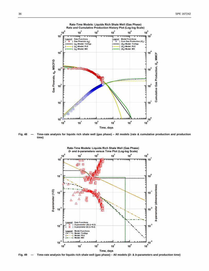
Results of the model fitting are summarized in Table 5, and the forecast and analysis plots are shown in Fig. 32 – Fig. 49. Comparisons of the EUR forecasts between the models are shown in Fig. 50 – Fig. 52. All three models generally match the production data. In all cases the MH is either the most liberal forecast, or tied for the most liberal forecast, with the exclusion of well B.6. For the TH, an attempt was made to use a bmax of 2.0 where possible to honor the value of the b-parameter observed in long duration linear flow. Not all the wells in this data set display such a trend. In those cases, a bmax has been chosen that results in the best fit. For the East Texas Tight Gas well, there appears to be an event that occurred at ~750 days, which disrupted the linear flow trend in the time-rate data. Consequently, it is difficult to gain insight from the fit of the TH. In this instance, it is possible to adjust the parameters of the equation and still obtain an excellent fit; however, the parameters will have little physical meaning. All three models forecast a similar EUR. With 5.5 years of production, there is not much uncertainty remaining in the forecast.

Well A.2 has a stable production history, and an initial b-parameter of 2.0 is distinguishable in the data. This allows the PLE to obtain an excellent fit for the transient flow regime. However, the production history ends in the middle of the transition period, and leaves the determination of the terminal decline rate uncertain. It is possible to apply a range of values to either the TH or the PLE, and the difference in EUR for this well should not be interpreted as material. The TH and PLE models are in disagreement for wells A.3 and C.2, cases where the bmax parameter of the TH is above 2. There is no clear evidence of the end of linear flow in well A.3, and without such evidence in the diagnostics, telf has been set as conservatively as possible. Well C.2 does indicate a transition to boundary-dominated flow, although uncertainty about bmin remains given the high, initial bmax. While an argument can be made for the uncertainty about when linear flow will end, this does highlight a shortcoming of the Transient Hyperbolic model – it does not perform with confidence when very little is known about the reservoir. It does, however, serve very well to set a bound for the minimum EUR by modeling the transition to boundary-dominated flow as soon as is possible, given the current data. Wells B.3 and B.6 are interesting in that they exhibit a linear flow duration that lasts less than 20 days. Both wells show excellent fits with the TH. However, the b-parameter is slowly increasing over time. This could be interpreted as extreme completion heterogeneity – depletion of the short-linear-flow-duration stages is occurring, and some fracture stages are still either in linear flow, or transitioning to boundary-dominated flow. This causes a bmin of 0.875 required to fit the data. Caution should be taken, though, as in light of the prior work illustrating completion heterogeneity in a MFHW, the b-parameter should eventually decrease over time. A forecast that does not represent this is very likely to over-estimate the EUR. The fits applied were purposefully chosen not to represent this in order to demonstrate a short-coming of relying solely on the model’s fits to current production history. Proper understanding of the effects of completion heterogeneity is paramount to a good forecast. Well C.3 has a spike in the value of the b-parameter, which makes the determination of bmax difficult. Several different values can all give comparable fits. The flow rate and D-parameter do display smooth trends, however, and allow an apparent good fit of the time-rate data. The PLE and TH result in nearly the same forecast for this well. The liquids rich shale well, in both the oil and gas phases, displays a very short duration of linear flow. The D-parameter on a log-log plot versus time follows a straight line trend, and the result is an excellent fit with the PLE. The TH model also

SPE 167242 9

demonstrates similar straight-line trends in each distinct flow regime, and displays an excellent fit as well. The forecast for the MH is very similar; however, it requires an estimate of the average b-parameter to fit over the life of the well – in this case a value of 0.8 – which cannot be known a priori. Wells A.2 and C.3 show similar fits of the data by all three models. Well A.2 has an initial b-parameter of 2.0 and a rather long linear flow duration, which allows the PLE to obtain a good fit. The TH fits well at all points. It is difficult to distinguish one being better than the other due. Well C.3 is difficult to fit with the PLE. The initial b-parameter of 1.2 represents an early-time, non-straight D-parameter trend on log-log versus time, and results in a curvature of the rate versus time function that is generally in trend with the data but varies from high to low at different points in time. Conclusion This paper has introduced the Transient Hyperbolic model as a method of forecasting production in tight gas and unconventional reservoirs. The basis for the model is the logistic transition of the Arps b-parameter as a means to represent the change between binary states in a confined space – different points in the reservoir are either infinite-acting or not, and the time for the transition to occur is proportional to the time at which the transition begins. In addition, the remaining parameters for the model are derivable from an analysis of time-rate production data. These parameters are commonly evaluated on various diagnostic plots currently used within the industry, and should also be familiar concepts to anyone applying the Modified Hyperbolic model. The logistic transition of the b-parameter was calibrated on numerical simulations consisting of multiple cases of an identical reservoir with varying length. It was then applied to model the various “divisions” in a MFHW with completion heterogeneity, which represent the various times at which areas of a reservoir reach t > telf. Each division was created with a bmin of 0.5. A “superposition” b-parameter as a function of time was calculated based on these divisions, and for a Transient Hyperbolic model of the entire well, a bmin of 0.7 was required to fit “superposed” b-parameter. This exercise shows that the predictions of the Transient Hyperbolic model match empirical observations of b-parameters of > 0.5 in MFHWs. A b-parameter > 0.5 is an emergent consequence of many layers or fracture stages, each having a differing duration of linear flow. Fits of several field cases were presented in comparison to two other decline curve models, to illustrate the behavior of the model. As always, caution should be taken to ensure one is not fitting noise in the data, or when there is not sufficient production history available. Fitting time-rate data “in a vacuum” is a difficult exercise and may lead to over- or underestimation. As telf controls the time at which terminal decline begins and is independent of initial rate or initial decline, there are an infinite number of unique solutions for telf when t < telf. For the field cases presented, telf was set as conservatively as possible, and bmin was set to a value of 0.7. Absence of information to indicate what the values for these parameters should be decreases the confidence of the model to correctly forecast production. However, the Transient Hyperbolic model can represent a lower bound on the production forecast that respects the physics of changing flow regimes. Despite difficulty in estimating the terminal decline parameters when no information is present, the physical meaning associated with its parameters is also the strength of the model. The telf parameter is a function of reservoir geometry via fracture spacing and reservoir properties. The bmin parameter is a function of completion heterogeneity via different fracture half-lengths in each fracture stage, or a layered reservoir. Ideally, given information on reservoir properties and reservoir geometry to predict these parameters, a practicing reservoir engineer should be able to accurately forecast production with only a few months to less than a year of production history. It should also be possible to more accurately forecast the impact of fracture spacing and fracture half-length on production rate. Such topics remain open for investigation in future work.

10 SPE 167242

Nomenclature Field variables

b = Arps’ hyperbolic decline exponent, dimensionless b′ = Derivative of Arps’ hyperbolic decline exponent, dimensionless bmax = maximum Arps’ b-parameter for Transient Hyperbolic time-rate model, dimensionless bmin = minimum Arps’ b-parameter for Transient Hyperbolic time-rate model, dimensionless c = Model coefficient (scaling factor) for Transient Hyperbolic time-rate model, dimensionless ct = Total compressibility, psi-1

d = Average fracture spacing, ft dj = Fracture spacing of pseudo-fracture division j, ft D = Reciprocal of the loss ratio, D-1 Di = Initial decline constant for the Transient Hyperbolic and Modified Hyperbolic time-rate models, D-1 D� i = Reciprocal of the loss ratio, D-1

D∞ = Reciprocal of the loss ratio, D-1

Ei = Exponential integral function, dimensionless EUR = Estimated ultimate recovery, BSCF or MBBL Gp = Cumulative gas production, MSCF or BSCF h = Reservoir thickness, ft kfw = Fracture conductivity, md-ft km = Matrix permeability, md Lw = Length of horizontal well, ft Np = Cumulative gas production, MBBL or BBL n = Time exponent for the Power-Law Exponential time-rate model, dimensionless pi = Initial reservoir pressure, psi pwf = Well flowing pressure, psi q = Production rate, MSCF/D or BBL/D qi = Initial rate for the Transient Hyperbolic and Modified Hyperbolic time-rate models, MSCF/D or BBL/D q� i = Initial rate coefficient for the Power-Law Exponential time-rate model, MSCF/D or BBL/D qj = Initial rate for division j in a heterogeneous completion, MSCF/D or BBL/D Sw = Water saturation, fraction t = Production time, days tDye = Dimensionless time based on reservoir length (ye) tehs = Time to end of half-slope on diagnostic plots, days telf = Time to end of linear flow, days tbdf = Time to boundary dominated flow, days xf = Fracture half-length, ft �̅�𝑓 = Average fracture half-length of pseudo-fractures, ft �𝑥𝑓�𝑚𝑎𝑥 = Maximum fracture half-length of pseudo-fractures, ft xe = Reservoir half-width (equal to fracture half-length), ft ye = Reservoir half-length (distance from fracture to boundary), ft

Greek variables αj = Ratio of drainage area in division j in a heterogeneous completion to the total drainage area, fraction βj = Ratio of pseudo-fracture half-length in division j in a heterogeneous completion to the maximum fracture

half-length, fraction γ = Euler-Mascheroni constant, 0.57722… µg = gas viscosity, cp ϕ = matrix porosity, fraction

Acknowledgements We thank Dave Symmons (consultant), Dilhan Ilk (DeGolyer and MacNaughton), and Paul Griffith (Apache Corporation) for their assistance with this work.

SPE 167242 11

References Arps., J.J.: “Analysis of Decline Curves,” Trans. AIME (1945) 160, 228.

Wattenbarger, R.A., El-Banbi, A.H., Villegas, M.E. and Maggard, J.B., 1998. “Production Analysis of Linear Flow Into Fractured Tight Gas Wells”, paper SPE 39931 presented at SPE Rocky Mountain Regional Low-Permeability Reservoirs Symposium and Exhibition in Denver, Colorado, 5-6 April, 1998

Spivey, J.P., Frantz Jr., J.H. Williamson, J.R., and Sawyer, W.R., 2001. “Applications of the Transient Hyperbolic Exponent”, paper SPE 71038 presented at SPE Rocky Mountain Petroleum Technology Conference in Keystone, Colorado, 21-23 May, 2001

Kupchenko, C.L., Gault, B.W., and Mattar, L., 2008. “Tight Gas Production Performance Using Decline Curves”, paper SPE 114991 presented at CIPC/SPE Gas Technology Symposium, Calgary, Alberta, Canada, 16-19 June, 2008

Ilk, D., Rushing, J.A., and Blasingame, T.A.., 2008. “Estimating Reserves Using the Arps Hyperbolic Rate-Time Relation – Theory, Practice and Pitfalls”, paper CIM 2008-108 presented at 59th Annual Technical Meeting of the Petroleum Society, Calgary, AB, Canada, 17-19 June, 2008

Ilk, D., Rushing, J.A., Perego, A.D., and Blasingame, T.A., 2008. “Exponential vs. Hyperbolic Decline in Tight Gas Sands – Understanding the Origin and Implications for Reserve Estimates Using Arps’ Decline Curves”, paper SPE 116731 presented at SPE Annual Technical Conference and Exhibition, Denver, Colorado, 21-24 September, 2008

Nobakht, M., Morgan, M., Matar, L., 2010. “Case Studies of a Simplified Yet Rigorous Forecasting Procedure for Tight Gas Wells”, paper SPE 117456 presented at the Canadian Unconventional Resources & International Petroleum Conference, Calgary, AB, Canda, 19-21 October, 2010

Ambrose, R.J., Clarkson, C.R., Youngblood, J., Adams, R., Nguyen, P., Nobakht, M., and Biseda, B., 2011, “Life-Cycle Decline Curve Estimation for Tight/Shale Gas Reservoirs”, paper SPE 140519 presented at SPE Hydraulic Fracturing Technology Conference and Exhibition, The Woodlands, Texas, 24-25 January, 2011

Nobakht, M., Ambrose, R., Clarkson, C.R., 2011, “Effect of Heterogeneity in a Horizontal Well With Multiple Fractures on the Long-Term Forecast in Shale Gas Reservoirs”, paper SPE 149400 presented at the Canadian Unconventional Resources Conference, Calgary, AB, Canada, 15-17 November, 2011

Okouma, V., Symmons, D., Hosseinpour-Zonoozi, N., Ilk, D., and Blasingame, T.A., 2012, “Practical Considerations for Decline Curve Analysis un Unconventional Reservoir – Application of Recently Developed Time-Rate Relations”, paper SPE 162910 presented at SPE Hydrocarbon, Economics, and Evaluation Symposium, Calgary, AB, Canada, 24-25 September, 2012

12 SPE 167242

Fig. 1 — Type curves of the Transient Hyperbolic Model, rate versus time for varying reservoir length (ye)

Fig. 2 — Type curves of the Transient Hyperbolic Model, rate versus material balance time for varying reservoir length (ye)

SPE 167242 13

Fig. 3 — Type curves of the Transient Hyperbolic Model, cumulative production versus time for varying reservoir length (ye)

Fig. 4 — Type curves of the Transient Hyperbolic Model, cumulative production versus material balance time for varying reservoir length (ye)

14 SPE 167242

Fig. 5 — Type curves of the Transient Hyperbolic Model, D-parameter versus time for varying reservoir length (ye)

Fig. 6 — Type curves of the Transient Hyperbolic Model, D-parameter versus material balance time for varying reservoir length

(ye)

SPE 167242 15

Fig. 7 — Type curves of the Transient Hyperbolic Model, b-parameter versus time for varying reservoir length (ye)

Fig. 8 — Type curves of the Transient Hyperbolic Model, b-parameter versus material balance time for varying reservoir length

(ye)

16 SPE 167242

Fig. 9 — a hydraulically fractured well in a rectangular reservoir with the fracture, xf extending the entirety of the reservoir

width xe

Fig. 10 — Numerical cases’ b-parameters versus 𝒕𝑫𝒚𝒆 (dimensionless time in the ye direction) for varying reservoir length (ye),

with fit of b(t) (Eq. 5)

SPE 167242 17

Fig. 11 — Fit of rate, D-parameter, and b-parameter for numerical case ye = 25 ft versus time

Fig. 12 — Fit of rate, D-parameter, and b-parameter for numerical case ye = 50 ft versus time

18 SPE 167242

Fig. 13 — Fit of rate, D-parameter, and b-parameter for numerical case ye = 75 ft versus time

Fig. 14 — Fit of rate, D-parameter, and b-parameter for numerical case ye = 100 ft versus time

SPE 167242 19

Fig. 15 — Fit of rate, D-parameter, and b-parameter for numerical case ye = 125 ft versus time

Fig. 16 — Fit of rate, D-parameter, and b-parameter for numerical case ye = 150 ft versus time

20 SPE 167242

Fig. 17 — Fit of rate, D-parameter, and b-parameter for numerical case ye = 175 ft versus time

Fig. 18 — Fit of rate, D-parameter, and b-parameter for numerical case ye = 200 ft versus time

SPE 167242 21

Fig. 19 — Fit of rate, D-parameter, and b-parameter for numerical case ye = 225 ft versus time

Fig. 20 — Fit of rate, D-parameter, and b-parameter for numerical case ye = 250 ft versus time

22 SPE 167242

Fig. 21 — Fit of rate versus time for all for numerical cases

Fig. 22 — Fit of cumulative production versus time for all for numerical cases

SPE 167242 23

Fig. 23 — Fit of D-parameter versus time for all for numerical cases

Fig. 24 — Fit of b-parameter versus time for all for numerical cases

24 SPE 167242

Fig. 25 — EUR Comparison plot – Transient Hyperbolic Model vs. Numerical Cases

Fig. 26 — Time-rate analysis of Mexico Tight Gas Well – fit of Transient Hyperbolic Model

SPE 167242 25

Fig. 27 — A MFHW with a heterogeneous completion with 14 fractures divided into seven divisions with different time to end of

linear flow (Modified from Nobakht et al [2011])

Fig. 28 — Time-rate analysis for superposition of pseudo-fractures in a heterogeneous completion – rate and production time

(All pseudo-fracture divisions)

26 SPE 167242

Fig. 29 — Time-rate analysis for superposition of pseudo-fractures in a heterogeneous completion – rate & cumulative

production and production time

Fig. 30 — Time-rate analysis for superposition of pseudo-fractures in a heterogeneous completion – b-parameter

SPE 167242 27

Fig. 31 — Time-rate analysis for superposition of pseudo-fractures in a heterogeneous completion – D-parameter

28 SPE 167242

Fig. 32 — Time-rate analysis for East Texas Tight Gas Well – All models (rate & cumulative production and production time)

Fig. 33 — Time-rate analysis for East Texas Tight Gas Well – All models (D- & b-parameters and production time)

SPE 167242 29

Fig. 34 — Time-rate analysis for well A.2 – All models (rate & cumulative production and production time)

Fig. 35 — Time-rate analysis for well A.2 – All models (D- & b-parameters and production time)

30 SPE 167242

Fig. 36 — Time-rate analysis for well A.3 – All models (rate & cumulative production and production time)

Fig. 37 — Time-rate analysis for well A.3 – All models (D- & b-parameters and production time)

SPE 167242 31

Fig. 38 — Time-rate analysis for well B.3 – All models (rate & cumulative production and production time)

Fig. 39 — Time-rate analysis for well B.3 – All models (D- & b-parameters and production time)

32 SPE 167242

Fig. 40 — Time-rate analysis for well B.6 – All models (rate & cumulative production and production time)

Fig. 41 — Time-rate analysis for well B.6 – All models (D- & b-parameters and production time)

SPE 167242 33

Fig. 42 — Time-rate analysis for well C.2 – All models (rate & cumulative production and production time)

Fig. 43 — Time-rate analysis for well C.2 – All models (D- & b-parameters and production time)

34 SPE 167242

Fig. 44 — Time-rate analysis for well C.3 – All models (rate & cumulative production and production time)

Fig. 45 — Time-rate analysis for well C.3 – All models (D- & b-parameters and production time)

SPE 167242 35

Fig. 46 — Time-rate analysis for liquids rich shale well (oil phase) – All models (rate & cumulative production and production

time)

Fig. 47 — Time-rate analysis for liquids rich shale well (oil phase) – All models (D- & b-parameters and production time)

36 SPE 167242

Fig. 48 — Time-rate analysis for liquids rich shale well (gas phase) – All models (rate & cumulative production and production

time)

Fig. 49 — Time-rate analysis for liquids rich shale well (gas phase) – All models (D- & b-parameters and production time)

SPE 167242 37

Fig. 50 — EUR Comparison plot between Transient Hyperbolic and Power-Law Exponential models

Fig. 51 — EUR Comparison plot between Transient Hyperbolic and Modified Hyperbolic models

38 SPE 167242

Fig. 51 — EUR Comparison plot between Power-Law Exponential and Modified Hyperbolic models

SPE 167242 39

Appendix A — Derivation of the "Transient Hyperbolic "Time-Rate Relation In this appendix we begin with the concept of a 2-step (maximum to minimum) hyperbolic time-rate relation that utilizes a logistic function to represent the path from the maximum to the minimum hyperbolic coefficients. While there are references that suggest this character (Kupchenko et al. [2009]), the work is proposed from the assumption that there is an arbitrary maximum hyperbolic coefficient (i.e., the Arps' "b-parameter") which transitions to a minimum hyperbolic coefficient over time. It is noted that the shape of the b-parameter suggested by Kupchenko et al is an asymmetric sigmoid function (i.e., “s-curve”) with varying rates of transition dependent upon the reservoir geometry. The proposed model is given by:

( ) [ ][ ][ ]γexpexp exp ) ( )( minmaxmax +−−−−−= elfttcbbbtb ........................................................................ (A-1)

Where bmax and bmin are the maximum and minimum hyperbolic coefficients, respectively, c is a scaling factor which controls the rate of transition, and telf is the time at which the transition begins (i.e., the time to end of linear flow). The prediction of the time at which the transition begins and ends has an analytic relationship to reservoir properties, allowing for the prediction of decline behavior. This relationship was first suggested by Wattenbarger et al (SPE 39931; 1998), and is built upon here. As a basis, we need to state the traditional definitions for the Arps rate relations — specifically (in modern nomenclature) we have the original Arps "loss ratio" and the "derivative of the loss ratio," which are given as:

Definition of the Loss Ratio:

dtdq

q

Da

/

1−≡≡ ................................................................................................................................................... (A-2)

Derivative of the Loss Ratio:

[ ]

−≡

≡≡

dtdq

q

dt

d

Ddt

dadt

db/

1 ................................................................................................................ (A-3)

Where:

a = The original Arps variable for the loss ratio D = The modern "decline" parameter (general) Di = Constant "decline" parameter

We can plot the b-parameter of our numerical cases (model properties are listed in Table 1) as a function of time and identify a consistent “shape” varied by the time to transition from bmax to bmin (derivatives are smoothed for presentation):

40 SPE 167242

Fig. A-1 — fit of b-parameter as a function of time for varying ye From these data in Fig. A-1 we can see that bmax = 2 and bmin = 0.38, with a consistent shape of transition yet varying times of transition. In the cases where ye is very small (25 ft – 75 ft), b(t) drops to zero after some period of time at bmin. These are numerical artifacts of the simulation at small values of q(t). As they occur very late in time for each case, and at very low flow rate (<10 MSCFD), they will not have a significant impact on forecasts of EUR. From Wattenbarger et al [1998] we can calculate a dimensionless time based upon ye (or ½ of the fracture stage spacing):

( ) 2

00633.0

eit

Dye

yc

tktµφ

= .................................................................................................................................................. (A-4)

We can plot the b-parameter of our numerical cases versus dimensionless time (tDye) and identify the time to end of linear

flow, telf, and the time to boundary dominated flow, tbdf. These are defined as when b(t) begins transition from bmax and settles at bmin, respectively. (see Table 1 for model properties):

SPE 167242 41

Fig. A-2 — Arps’ b-parameter as a function of dimensionless time (tDye) From Fig. A-2 we can identify telf and tbdf:

1.0, =elfDyet .............................................................................................................................................................. (A-5)

7.0, =bdfDyet ............................................................................................................................................................. (A-6)

We can also identify a fixed relationship between the two; that is, tbdf is a function of telf.

( ) elfelfelf

elfDye

bdfDyeelfbdf ttt

t

ttt 0.7

1.0

7.0 ,

, === ........................................................................................................... (A-7)

Solving for time (t) in Eq. A-4 gives us:

( )

k

yctt etDye

00633.0

2µφ= ................................................................................................................................................... (A-8)

And substituting in our values for telf in Eq. A-5 and tbdf in Eq. A-6 results in:

( )

k

yct etelf

0633.0

2µφ= ...................................................................................................................................................... (A-9)

( )

k

yct etbdf

004431.

2µφ= .................................................................................................................................................. (A-10)

To derive Eq. A-1, we must first start with the general form of the Gompertz, written as:

( ) ( ) ( ) ( )[ ][ ]tcbaty −−= expexp .................................................................................................................... (A-11)

Where a is the final value, b is the displacement factor, and c is the scaling factor.

42 SPE 167242

Substituting Arps’ equation parameters gives:

( )minmaxmax bbba −−=

[ ][ ]γexpexp=b

cc =

( ) ( ) [ ] [ ][ ][ ]tcbbbtb −−−−= expexpexpexpminmaxmax γ ............................................................................ (A-12)

The final value, a, is the difference between the starting value and the desired final value. The Gompertz function is a monotonically decreasing function, so for this application it must be inverted and vertically displaced. The displacement factor, b, is an empirically derived adjustment factor to cause the beginning of the transition to occur at the desired time t. It shifts the inflection point of the function, causing transition to begin at t = 0 rather than the inflection point to coincide at t = 0. It is moved inside the second exponentiation for simplicity:

( ) ( ) [ ][ ][ ]γexpexpminmaxmax +−−−−= tcexbbbtb ................................................................................... (A-13)

This form of the b(t) function will begin the transition from bmax at t = 0. As we have the actual time at which this transition begins from Eq. A-9, we can add the telf term to act as a “trigger” so that the transition begins at t = telf.

( ) ( ) ( ) [ ][ ][ ]γexpexpexpminmaxmax +−−−−−= elfttcbbbtb ...................................................................... (A-1)

The scaling factor, c, provides the rate of transition of the function from bmax to bmin, and is dependent not on the value of telf, but on the difference between telf and tbdf , and the values of bmax and bmin. It must have a specific value for any given set of parameters for Eq. A-1, and a full derivation of c can be found in Appendix B. Summarizing so far:

( )

k

yct etelf

0633.0

2µφ= ...................................................................................................................................................... (A-9)

[ ]

elftc

5.1

exp γ= ................................................................................................................................................................ (B-1)

( ) [ ][ ][ ]γexpexp exp ) ( )( minmaxmax +−−−−−= elfttcbbbtb ........................................................................ (A-1)

Derivation of Transient Hyperbolic Rate Decline Case: Starting with Eq. A-5 (slightly rearranged), we have:

)(1 tbDdt

d=

....................................................................................................................................................... (A-14)

Substituting Eq. A-1 into Eq. A-14 yields:

( ) [ ][ ][ ]γexpexp exp ) ( 1minmaxmax +−−−−−=

elfttcbbb

Ddt

d ................................................................. (A-15)

Separating the decline (D) and time (t) variables — then setting up an "indefinite integration" of Eq. A-15, we obtain:

( ) [ ][ ][ ]∫∫∫ +−−−−−= dtttcbbdtbD

d elf γexpexp exp ) ( 1minmaxmax ................................................. (A-16)

Integrating by substitution, where:

SPE 167242 43

( ) [ ][ ]γexpexp +−−−= elfttcu ......................................................................................................................... (A-17)

( ) [ ][ ][ ] dtttcddu elf γexpexp +−−−=

We must use the chain rule to find the derivative of u:

[ ] dtdu

dv

dv

vddu exp−= ......................................................................................................................................... (A-18)

Where:

( ) [ ]γexp+−−= elfttcv ....................................................................................................................................... (A-19)

[ ] [ ]vvdv

d expexp =

Taking the derivative of Eq. A-18 yields:

[ ] dtdu

dvvdu exp−= .............................................................................................................................................. (A-20)

And substituting Eq. A-19 produces:

( ) [ ][ ] ( ) [ ][ ] dtttcdu

dttcdu elfelf γγ expexpexp +−−+−−−= ................................................................. (A-21)

Separating terms of Eq. A-21:

( ) [ ][ ] [ ] dtdu

dtcdu

dtcdu

dttcdu elfelf

++−+−−−= γγ expexpexp ..................................................... (A-22)

Taking the derivate of each term gives us:

( ) [ ][ ] ( ) ( ) ( )[ ]dtcttcdu elf 00expexp ++−+−−−= γ ................................................................................... (A-23)

And we can reduce Eq. A-23 to:

( ) [ ][ ]dtttccdu elf γexpexp +−−=

( ) [ ][ ]γexpexp +−−=

elfttcc

dutd .................................................................................................................... (A-24)

We can then substitute Eq. A-17 into Eq. A-24

uc

dutd −= ............................................................................................................................................................... (A-25)

Substituting Eqs. A-17 & A-25 into Eq. A-16 and slightly re-arranging yields:

[ ]

−−−= ∫∫∫

uc

duubbdtbD

d exp ) ( 1minmaxmax ....................................................................................... (A-26)

We can re-arrange Eq. A-26:

[ ]∫∫∫

−+=

u

duubbdtbD

d exp c

) ( 1 minmaxmax ............................................................................................ (A-27)

44 SPE 167242

Which yields the Exponential Integral, defined as:

( ) [ ] duu

uuEi ∫=exp

............................................................................................................................................. (A-28)

Integrating Eq. A-27 produces:

[ ] CubbtbD

+−

+= Eic

) ( 1 minmaxmax ................................................................................................................. (A-29)

Substituting Eq. A-17 into Eq. Eq. A-29 gives us:

( )( ) [ ][ ][ ] Cttc

c

bbtbtD

elf ++−−−

+= γexpexp- Ei) ( 1 minmaxmax .............................................................. (A-30)

Evaluation of Eq. A-30 at zero time (i.e., t = 0) allows us to solve for the "initial" (or constant) value of the D-parameter (i.e., Di). Specifically, we have:

( ) [ ][ ][ ] Ctcc

bbbD

elf

i

++−−−

+= γexp)0(exp- Ei) ( )0(1 minmaxmax

[ ][ ][ ] Ctcbb

Delf

i

++−

= γexpexp- Eic

) ( 1 minmax ........................................................................................... (A-31)

Solving for the C coefficient gives us:

[ ][ ][ ]γexpexp- Ei) (1 minmax +−

−= elf

i

tcc

bb

DC ......................................................................................... (A-32)

Substitution of Eq. A-32 into Eq. A-30 yields:

( )( ) [ ][ ][ ] [ ][ ][ ]γγ expexp- Ei

) (expexp- Ei

) ( 11 minmaxminmax

max +−

−+−−−

++= elfelf

i

tcc

bbttc

c

bbtb

DtD .. (A-33)

We can simplify Eq. A-33 to:

( )( ) [ ][ ][ ] [ ][ ][ ][ ]γγ expexp- Eiexpexp- Ei) ( 11 minmax

max +−+−−−

++= elfelf

i

tcttcc

bbtbDtD

..... (A-34)

And taking the reciprocal:

( )( ) [ ][ ][ ] [ ][ ][ ][ ]γγ expexp- Eiexpexp- Ei) ( 1

1minmax

max +−+−−−

++=

elfelf

i

tcttcc

bbtbD

tD ...... (A-35)

Recalling Eq. A-3:

[ ]

−≡

≡≡

dtdq

q

dt

d

Ddt

dadt

db/

1 ................................................................................................................ (A-3)

Taking the reciprocal of Eq. A-3 (we note that D ≡ D(t)):

dt

dq

qtD 1)( ≡− ....................................................................................................................................................... (A-36)

SPE 167242 45

And substituting Eq. A-35 into Eq. A-36 and separating the rate (q) and time (t) variables:

( ) [ ][ ][ ] [ ][ ][ ][ ]dt

tcttcc

bbtbD

dqq elfelf

i

γγ expexp- Eiexpexp- Ei) ( 111

minmaxmax +−+−−

−++

−= ... (A-37)

Integrating Eq. A-37 gives us:

( ) [ ][ ][ ] [ ][ ][ ][ ]dt

tcttcc

bbtb

D

tdq

q

q

qelfelf

i

i γγ expexp- Eiexpexp- Ei) (

11

0

1minmax

max +−+−−−

++−= ∫∫ ... (A-38)

Although the integral in Eq. A-38 cannot be reduced, we can solve this relation for the flow rate, which yields:

( )( ) [ ][ ][ ] [ ][ ][ ][ ]

+−+−−−

++−= ∫ dt

tcttcc

bbtb

D

tqtq

elfelf

i

i

γγ expexp- Eiexpexp- Ei) (

11

0exp

minmaxmax

... (A-39)

As a check, if bmax = bmin = b, then Eq. A-39 becomes:

( ) [ ][ ][ ] [ ][ ][ ][ ]

+−+−−++−= ∫∫ dt

tcttcc

btD

tqdq

q

q

qelfelf

i

i

i γγ expexp- Eiexpexp- Ei)0( 11

0exp 1 ... (A-40)

Where we have the following final reduction:

dttbD

tDdq

q

q

qi

i

i 1

1 0

1

+−= ∫∫ ...................................................................................................................... (A-41)

Where Eq. A-41 is exactly the same result as the typical hyperbolic decline case.

46 SPE 167242

Appendix B — Derivation of the Scaling Factor, c In this appendix we derive the value for the scaling factor, c, in the Transient Hyperbolic time-rate relation. It is observed in the numerical cases that tDye,elf and tDye,bdf are functions of reservoir properties and not rate (q) or time (t), and bmax and bmin are consequences of the flow regime before tDye,elf and after tDye,bdf, respectively. We can therefore deduct that b(tDye) is deterministic, and b(t) must have a unique solution for any given values of reservoir properties (porosity (ϕ), permeability (k), viscosity (γ), and total compressibility (ct)). c can be described as a calibration parameter to cause the b(t) function to reach bmin at tbdf, and must also have a unique solution. For the b(t) function to fit the observed data, c must first be properly calibrated. The proposed calibration of c is given by:

[ ]

elftc

5.1

exp γ= ................................................................................................................................................................ (B-1)

Recalling Eq. A-1.

( ) [ ][ ][ ]γexpexp exp ) ( )( minmaxmax +−−−−−= elfttcbbbtb ......................................................................... (A-1)

Rearranging Eq. A-1:

( ) [ ][ ][ ]γexpexpexpminmax

max +−−−=−

−elf

t ttcbb

bb ................................................................................................. (B-2)

Taking the natural log gives us:

( ) [ ][ ]γexpexplnminmax

max +−−−=

−

−elfttc

bb

btb ................................................................................................ (B-3)

Switching signs yield:

( ) [ ][ ]γexpexplnmax

minmax +−−=

−

−elf

t

ttcbb

bb ..................................................................................................... (B-4)

Taking the natural log again:

( ) [ ]γexplnlnmax

minmax +−−=

−

−elf

t

ttcbb

bb ..................................................................................................... (B-5)

And finally, solving for c results in:

[ ]

elf

t

tt

bb

bb

c−

+

−

−−

=

γexplnlnmax

minmax

.................................................................................................................. (B-6)

This function is undefined at t = telf, and tbdf, as b(telf) = bmax, and b(tbdf) = bmin, However, because the “shape” of the b(t) function is constant and independent of c (which only determines the rate of transition), and we can observe from Eq. B-6 that we can describe c given any pair of b(t) and t values, we can use the inflection point of the b(t) function as a constant time and value of b(t) to calibrate c.

SPE 167242 47

Starting with Eq. A-1:

( ) ( ) ( ) [ ][ ][ ]γexpexpexpminmaxmax +−−−−−= elfttcbbbtb ...................................................................... (A-1)

And setting up a derivative of Eq. A-1:

( ) ( ) ( ) [ ][ ][ ][ ]γexpexpexpminmaxmax +−−−−−=′ elfttcbbbdt

dtb

Separating terms yields:

( ) ( ) ( ) [ ][ ][ ][ ]γexpexpexpminmaxmax +−−−−−=′ elfttcbbdt

dbdt

dtb ........................................................ (B-7)

The derivative of bmax is zero:

( ) ( ) ( ) [ ][ ][ ][ ]γexpexpexp0 minmax +−−−−−=′ elfttcbbdt

dtb .................................................................. (B-8)

Using the chain rule:

( ) [ ]

dt

du

du

udbbtb exp)( minmax −−=′ ..................................................................................................................... (B-9)

Where:

( ) [ ][ ]γexpexp +−−−= elfttcu ........................................................................................................................(B-10)

[ ] [ ]uudu

d expexp =

Taking the derivative of Eq. B-9 gives us:

( ) [ ]dt

duubbtb exp)( minmax −−=′ ........................................................................................................................(B-11)

And substituting Eq. B-10 into Eq. B-11 produces:

( ) ( ) [ ][ ][ ] ( ) [ ][ ][ ]γγ expexpexpexpexp)( minmax +−−−+−−−−−=′ elfelf ttcdt

dttcbbtb ..................(B-12)

Using the chain rule again:

( ) ( ) [ ][ ][ ] [ ]

−+−−−−−=′

dt

du

du

udttcbbtb elfexpexpexpexp)( minmax γ ..............................................(B-13)

Where:

( ) [ ]γexp+−−= elfttcu ......................................................................................................................................(B-14)

[ ] [ ]uudu

d expexp =

Taking the derivative of Eq. B-13 gives us:

( ) ( ) [ ][ ][ ] [ ]

−+−−−−−=′

dt

duuttcbbtb elf expexpexpexp)( minmax γ ......................................................(B-15)

48 SPE 167242

Separating terms produces:

( ) ( ) [ ][ ][ ] [ ][ ]

−+−−−−−=′

dt

duuttcbbtb elf expexpexpexp)( minmax γ ...................................................(B-16)

And solving for the derivative of u (far right term of Eq. B-16) results in:

( ) [ ][ ]γexp+−−= elfttcdt

d

dt

du ..........................................................................................................................(B-17)

Separating terms gives us:

[ ] 00exp ++−=++−= cdt

dtcdt

dtcdt

d

dt

duelf γ ............................................................................................(B-18)

And substituting Eq. B-18 into Eq. B-16:

( ) ( ) [ ][ ][ ] ( ) [ ][ ][ ][ ]cttcttcbbtb elfelf −+−−−+−−−−−=′ γγ expexpexpexpexp)( minmax ...............(B-19)

Re-arranging Eq. B-19 yields:

( ) ( ) ( ) [ ][ ] ( ) [ ]( )[ ]γγ expexpexpexpminmax +−−++−−−−−=′ elfelf ttcttcbbctb .............................(B-20)

We can plot b′ of the numerical cases against dimensionless time, shown in Fig. B-1 and determine the inflection point:

Fig. B-1 — b′(t) as a function of dimensionless time

SPE 167242 49

Fig. B-2 — b(t) and b′(t) as a function of dimensionless time We observe in Fig. B-1 that the inflection point always occurs at:

25.0inf, =Dyet ..........................................................................................................................................................(B-21)

This can also be related to telf:

( ) elfelfelf

elfDye

bdfDyeelf ttt

t

ttt 5.2

1.0

25.0 ,

,inf === .........................................................................................................(B-22)

Substituting Eq. B-21 into Eq. A-8 yields:

( )

k

yct et

02532.0

2

infµφ

= ....................................................................................................................................................(B-23)

Next we must identify the value of b(tinf). If we consider the general form of the Gompertz function, c solely controls the rate of transition from the upper asymptote to the lower asymptote, illustrated in Fig. B-3.

50 SPE 167242

Fig. B-3 — general Gompertz function at various values of c

This is relevant because it means that the value of b(tinf) at the inflection point is independent of c. If we start with the general form of the Gompertz function:

( ) ( ) ( ) ( )[ ][ ]tcbaty −−= expexp .................................................................................................................... (A-11)

And we invert the function to transition from 1 to 0, substituting 1 for a, b, and c we obtain:

( ) ( ) ( ) ( )[ ][ ]tty 1exp1exp11 −−−=

And if we solve this function at time t = 0, it yields:

( ) [ ][ ] [ ]e

y 111exp10expexp10 −=−−=−−= .............................................................................................(B-24)

This value is proportional to the difference between the upper and lower asymptotes, and is independent of c. Therefore, the value of b(tinf) is deterministic and independent of c for any fixed bmax and bmin, and can be given by:

( ) minminmaxinf )(11 bbbe

tb +−

−= ..................................................................................................................(B-25)

Substituting Eq. B-22 and Eq. B-25 into Eq. B-6 yields:

[ ]( )[ ]

elfelf tt

bbbeb

bb

c−

+

+−−−

−−

=5.2

exp)(11

lnlnminminmaxmax

minmax γ

............................................................(B-26)

SPE 167242 51

We can rearrange Eq. B-26 to:

[ ][ ]

elfelf tt

bbebb

bb

c−

+

−−−−

−−

=5.2

exp)(11

lnlnminmaxminmax

minmax γ

................................................................(B-27)

And then reduce to:

( )

( ) [ ]( )[ ]

[ ][ ] [ ]

elfelfelfelf tt

e

tt

ec−

+−=

−

+

−−−

=5.2

explnln

5.2

exp1111

1lnlnγ

γ

.......................................................(B-28)

Which can be further reduced to:

[ ]

elftc

5.1

exp γ= .............................................................................................................................................................. (B-1)

Which yields the scaling factor, c.