Copyright 2006, Society of Petroleum Engineers

This paper was prepared for presentation at the 2006 SPE Annual Technical Conference andExhibition held in San Antonio, Texas, U.S.A., 24–27 September 2006.

This paper was selected for presentation by an SPE Program Committee following review ofinformation contained in an abstract submitted by the author(s). Contents of the paper, aspresented, have not been reviewed by the Society of Petroleum Engineers and are subject tocorrection by the author(s). The material, as presented, does not necessarily reflect any positionof the Society of Petroleum Engineers, its officers, or members. Papers presented at SPEmeetings are subject to publication review by Editorial Committees of the Society of PetroleumEngineers. Electronic reproduction, distribution, or storage of any part of this paper for commercialpurposes without the written consent of the Society of Petroleum Engineers is prohibited.Permission to reproduce in print is restricted to an abstract of not more than300 words; illustrations may not be copied. The abstract must contain conspicuousacknowledgment of where and by whom the paper was presented. Write Librarian, SPE, P.O. Box833836, Richardson, TX 75083-3836, U.S.A., fax 01-972-952-9435.

Abstract

Although production analysis (PA) for reservoir characterizationis approaching the popularity of pressure transient analysis(PTA), there are few consistent diagnostic methods in practicefor the analysis of production data. Many of the "diagnostic"methods for production data analysis are little more thanobservation-based approaches — and some are essentially "rulesof thumb."

In this work we provide guidelines for the analysis of productiondata, as well as identify common pitfalls and challenges.Although pressure transient and production data analyses havethe same governing theory (and solutions), we must recognizethat pressure transient data are acquired as part of a controlled"experiment," performed as a specific event [e.g., a pressurebuildup (or PBU) test]. In contrast, production data aregenerally considered to be surveillance/monitoring data — withlittle control and considerable variance occurring during theacquisition of the production data.

This paper attempts to provide a "state-of-the-technology"review of current production data analysis techniques/tools —particularly tools to diagnose the reservoir model and assess thereservoir condition. This work also identifies the challenges andpitfalls of production analysis — and we try to provide guidancetowards best practices and best tools. To compliment thismission, we use relevant field examples to address specificissues, and we illustrate the value and function of productiondata analysis for a wide range of reservoir types and properties.

Prologue

A rudimentary assessment might conclude that pressure transientdata are "high frequency/high resolution" data — and productiondata are "low frequency/low resolution" data. This would be anoversimplified view, but in practice, the fact is that productiondata rarely approach the quality, quantity, or accuracy of dataacquired during a pressure transient test. Another "generali-zation" that holds considerable truth is that during a pressure

transient test, the pressure data are typically measured at extra-ordinary frequencies (points/second) and accuracies (pressure to1 part in 100,000 per pressure range of the gauge) — while theproduction history is either ignored, or is derived from "back ofthe envelope" estimates or cursory reviews of the recent produc-tion history.

An inverted generalization often occurs for production data —the rate history is carefully obtained from daily records (or salessheets), and the pressure history is infrequent, inaccurate, and/oroften non-existent. The challenge of creating a coherent analysisfrom production data remains that of understanding what infor-mation the data may or may not be able to convey. For example,as transient flow data are required to estimate reservoir pro-perties, one should not expect to be able to estimate permeabilityand skin factor with confidence using monthly production ratesand pressures from a well in a moderate to high permeability re-servoir. These data simply lack the detail (i.e., the transient his-tory) to provide a competent analysis. In contrast, monthly pro-duction data may be sufficient for wells in low permeabilityreservoirs where the transient state may be maintained formonths or even years (although we would certainly prefer tohave at least a daily record of production rates and pressures).

Due Diligence — Literature

The literature for production analysis (PA) can be distilled intothe following categories and elemental references:

Basic Analysis of Production Data: The Arps work (ref. 1) wasthe systematic first attempt to correlate production data in thepetroleum literature and is considered to be an essential startingpoint for analysis. Mattar and McNeil2 provide a coupling ofmaterial balance and pseudosteady-state flow theory whichprovides an analysis/interpretation methodology for productiondata on a per-well basis. Li and Horne3 provide a recent attemptto "legitimize" production analysis by providing a theoreticalbasis (where possible) for several of the more commonproduction analysis relations.

Blasingame and Rushing4 provide a synopsis of the historicalmethods used for simplified production analysis and lend sometheoretical support for common applications (e.g., theexponential and hyperbolic decline relations, as well as semi-analytical solutions for gas flow). Ref. 5 by Camacho andRaghavan, while not a production data analysis reference bydesign, provides the theoretical basis for boundary-dominatedflow in solution gas-drive reservoirs — and should be consi-dered to be an essential reference on production analysis.

Decline Type Curve Analysis: The required reference forproduction decline curve analysis using type curves is theoriginal work on the subject by Fetkovich.6 The analytical basisand "integral" plotting functions for variable-rate/variablepressure drop production data are provided by Palacio and

SPE 102048

Production Data Analysis — Challenges, Pitfalls, DiagnosticsD. M. Anderson, G.W.J. Stotts, L. Mattar, Fekete Associates Inc.,D. Ilk, and T. A. Blasingame, Texas A&M U.

2 D. M. Anderson, G.W.J. Stotts, L. Mattar, D. Ilk, and T. A. Blasingame SPE 102048

Blasingame7 (for gas wells) and Doublet and Blasingame8 (foroil wells).

These variable-rate/variable pressure drop methodologies wereextended to fractured wells by Agarwal et al.9 and Araya andOzkan10 provide important perspectives on the use of productiondecline type curve analysis for vertical, fractured, and horizontalwells. Recently (2004), Fuentes-C. et al.11 provide extensionsof the decline type curve analysis approach for a variety of casesin naturally fractured reservoirs.

Diagnostic Methods for Production Data Analysis: There existsa dearth of literature on the specific topic of diagnostics withregard to production analysis. By contrast, the literature isreplete with references on the diagnostic analysis of pressuretransient test data. This situation exists because, as noted earli-er, pressure transient test data are considered to be "high fre-quency/high resolution" data that can yield a unique characterfor a particular well/reservoir condition. Production data areviewed as "low frequency/low resolution" data — and the ana-lysis of production data is labeled by some antagonists as the"analysis of clouds." While such a view is a bit cynical, there istruth to the perception that the diagnosis of production data ismuch more art than science.

Mattar and Anderson12 and Anderson and Mattar13 provideguidelines and examples for the diagnosis of production datawith regard to model-based analysis (type curves). Kabir andIzgec14 provide guidance on the diagnosis pressure-rate data.with an emphasis on characterizing the reservoir production me-chanism. Lastly, Bondar15 summarizes the modern and histori-cal methods of analyzing water-oil-ratio (WOR) and water cut(fw) data from the perspective of characterizing the reservoirdrive mechanism(s) and estimating reserves.

Expectations — Production Data Diagnosis

Using the guidelines/procedures presented in this work, a typicalanalyst should expect to be able to perform the following tasksusing a given set of production data:

Assess Data Viability: (i.e., preliminary data review) Determinewhether or not a particular production data set can (or cannot)be analyzed based the availability of:—Historical production data (rates and pressures).—Reservoir and fluid data (for quantitative analysis).—Well records (completion/stimulation history).

Check for Data Correlation: This is the intermediate stepbetween acquisition and analysis — a final review before thedata are processed and prepared for analysis. Recommendedtasks include:—Data correlation check (pwf (or ptf) vs. rate plot). This is an

extraordinarily simple check, but data which have no cor-relation probably will not provide any diagnostic value (otherthan to serve as a sign not to proceed).

—Rate-time and pressure-time plots — these can show featuresor events which should be filtered or discarded, a good exam-ple is that of well cleanup which could be (and usually is)due to poor early measurements.

Preliminary Diagnosis: This task considers the following diag-nostic aspects:— Identifying flow regimes (i.e., the reservoir model).—Data filtering for clarity (elimination of spurious data).—Data review/editing (e.g., well cleanup, recompletions).

Model-Based Analysis: In some ways, this is the "easiest" partof production data analysis — analogous to well test analyses;comparison/matching with well/reservoir models, refinement,then (if desired) — production forecasting. In this work we willsimply note that the references (in particular, refs. 1-11) provide

guidance with regard to historical and modern methods ofproduction data analysis, and we encourage the reader to consultsuch references for the actual tasks involved in model-basedanalysis (and forecasting).

The emphasis of this paper is the diagnosis of production data —as such, we will avoid the details of tasks related to model-basedanalysis, and we instead focus on the qualitative review andquantitative diagnostics of production data.

We do note that the most substantive diagnostic tool is ulti-mately the reservoir model — whether provided for as "typecurves" characteristic graphical solutions for a particular reser-voir model, or simply in the form of a simulation model whichwill be tuned to the data. Regardless of the form of the reservoirmodel (type curve or simulation module), the comparison of theproduction data with a consistent reservoir model is an essentialtask in the diagnosis of production data.

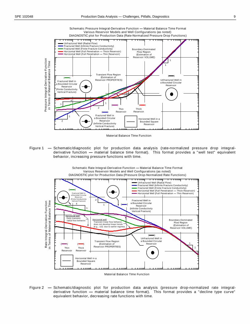
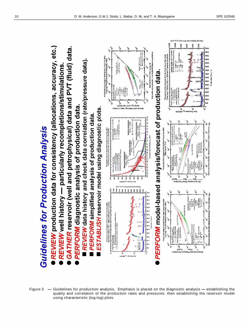
Figs. 1 and 2 provide a schematic view (a sort of "cartoon" typecurve) for common reservoir models, where evidence of tran-sient and boundary-dominated flow periods presented. Figs. 1and 2 show the "equivalent" constant rate schematic — Fig. 1 il-lustrates a "well test analysis" analog [(p/q) integral-derivativefunctions9], while Fig. 2 is a "production decline" view of thedata [(q/p) integral-derivative functions8]. For clarification,these data functions are derived from exactly the same reservoirmodel (in particular, the constant rate response) and are simplyplotted in these formats due to historical preferences. There isno "strategic" advantage to using either format [(p/q) or (q/p)]— and we encourage the user to become familiar with both for-mats and to recognize that each format has distinct characteristicfeatures that may provide assistance in the diagnosis procedure.For reference, the (p/q) functions are often referred to as the"normalized productivity index" format, and the (q/p) functionsare commonly referred to as the "Blasingame" format. As notedearlier, either format is satisfactory, and we encourage the userto use both formats to ensure that maximum diagnostic value isderived from the production data.

Guidelines for Production Analysis

While no "set" of guidelines for production analysis should everbe considered absolute, we do believe that consistency is essen-tial in the data gathering and data review process. Further, thediagnostic ("pre-analysis") phase of production analysis shouldnever be treated as rote — it is vital that the analyst treat everyanalysis as independent. The analyst must use all of the data attheir disposal to develop a "diagnostic" understanding of the pro-duction scenario, as well as the use these data to develop acharacteristic understanding of the reservoir model.

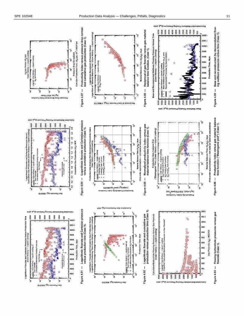
Fig 3 provides a graphic "guidebook" of tasks for the genericdiagnosis of production data. The emphasis is in this graphic isthe vigilant acquisition and "correlation" of the production his-tory, establishing the influence of the well completion history,and providing a diagnosis of the production character (and theviability of an analysis) — before any "analysis tasks" are per-formed.

Non-Graphical Diagnostics of Production Data

Comment: The analysis of production data to determine reservoircharacteristics, completion effectiveness, and hydrocarbons-in-place has become very popular in recent years. The "modern"era of production decline type curve analysis and model-based

SPE 102048 Production Data Analysis — Challenges, Pitfalls, Diagnostics 3

matching is well-documented (refs. 6-11). Production analysiscontinues to be validated as a reservoir characterization tool byfield application — particularly with the advent of continuousmeasurement (surface and downhole pressure measurements,continuous surface rate and pressure measurements, etc.).

Simply put, the data makes the analysis. For competentproduction data (e.g., accurate, continuous rate and pressuremeasurements where the well completion has not been altered),we can and should expect to be able to:Diagnose (establish) the reservoir/well model.Estimate reservoir properties (e.g., k, xf, Lw, etc.).Estimate the initial flow efficiency (and possibly the current

flow efficiency via history matching).Estimate in-place fluid volumes.

Obviously all models — analytical or numerical, have as-sumptions and limitations — and the production analysis met-hods currently in use are no exception. These methods reflectidealized conditions, and accordingly, the diagnosis and resultsof a particular data set are subject to these assumptions and limi-tations. Quite often such assumptions can be justified, and mea-ningful interpretations and results are obtained — particularlywhen the data set is as complete as possible — and the data areconsistent and of good quality.

As a reminder, in everyday practice, there are a significantnumber of production scenarios where the quality of the data isquestionable, inconsistent, and sometimes just plain wrong. Ex-perience plays a crucial role, and the current enthusiasm for pro-duction data analysis is hampered by a lack of resources whichprovide guidance to the analyst. Further, in the absence of suchinformation, many analysts become self-taught, which in manyregards is commendable. However; in our experience, a self-taught analyst (generally on virtually any subject, but parti-cularly with regard to production analysis) almost always limitsthemselves to the domain where their knowledge was obtained.

For example, an analyst who may be very proficient at analyzingthe performance of tight gas wells may be unprepared for casesof horizontal oil wells. Why elaborate so with regard to experi-ence? Quite simply, because the analyst is their own worstenemy when it comes to production data analysis/interpretation.The expectation that a particular data set can, and will, at allcosts be analyzed has led to cases of very poor analysis (even bythe authors of this work). This is especially true in cases of in-consistent, uncorrelated data. An "experienced" analyst willknow the tricks of the trade (particularly the software) and will,almost by definition, achieve an analysis that appears perfect. Anovice analyst will often not consider the physics of the process(or data quality issues) and will exhaustively try to obtain ananalysis/interpretation. And because of the robustness of thesolutions and the ease of use of commercial software, an exhaus-tive approach will eventually yield an analysis/interpretation —where the results may have little or no relation to the actual pro-perties of the system.

Experience is a valuable tool — but not a foolproof one. Allanalysts are encouraged to use a deliberate and consistent set ofprocedures — one that ensures that experience will not triumphover reason. Consider that most of the work performed by anairline pilot consists of pre-flight and post-flight checks — fly-ing is relatively easy (and enjoyable) by comparison. The same

can be said for production analysis — all of the tedious work isin the problem set-up and the post-mortem check — the ana-lysis/interpretation portion is arguably the least tedious part ofthe production analysis sequence.

In summary, a prudent analyst will always be skeptical withregard to production data (especially the pressure data and, to alesser degree, the well completion history) — and said analystwill always recheck the reservoir and fluid data as these arerequired input data. There is no guarantee that such efforts willkeep the analyst clear of a bad analysis/interpretation, but theseefforts will greatly reduce erroneous analyses.

Obviously our comments with regard to production analysisapply equally to pressure transient analysis — but, in the case ofpressure transient analysis, the focus is on a controlled, small-scale event which typically contains a very large set of high-precision measurements (i.e., the pressure data). Due to theevent scale and the quantity/quality of the measurements, theanalysis and interpretation of pressure transient data is almosteasy by comparison to the process for production data.

Common Challenges/Pitfalls: There is no closed set that canaccurately encompass all of the challenges and pitfalls that onemight encounter in production data analysis. However, there arecertainly some issues which are worse, or at least more pre-valent, than others. A sample of the more common challen-ges/pitfalls which occur in the analysis/interpretation of pro-duction data are:

IssueInfluence/Severity

Pressure:—No pressure measurement(s)—Incorrect initial pressure estimate—Poor ptf → pwf conversion (models)—Liquid loading: effect on ptf → pwf conversion—Incorrect location of pressure measurement

HighHighModerateModerateVery High

Flowrate:—Rate allocations (potential for errors)—Liquid loading: effect on gas flowrate

ModerateModerate

Well Completion:—Zone changes: new/old perforations—Changes in the wellbore tubulars—Changes in surface equipment—Stimulation: hydraulic fracturing—Stimulation: acidizing, etc.

Very HighHighMod./HighHighModerate

General:— Reservoir properties (, h, rw, cf, ct, etc.)— Oil properties: Bo, Rso, o, co, etc.— Gas properties: g, T, z (or Bg), g, cg, etc.— Poor time-pressure-rate synchronization— Poor time-pressure-rate correlation

ModerateModerateModerateMod./HighVery High

Understanding these issues is critical — if a production analysissequence is to be conducted, these issues must be recognized ifnot addressed.

We can separate the analysis of production data into twoseparate initiatives — the estimation of reservoir properties fromtransient flow data and the estimation of reservoir volume fromboundary-dominated flow data. Perhaps the most importantissue for the estimation of reservoir properties is to acknowledgethat legacy production data (i.e., data which are 20+ years old)may contain neither the quality, nor the frequency sufficient toproduce competent estimates of reservoir properties. In short, it

4 D. M. Anderson, G.W.J. Stotts, L. Mattar, D. Ilk, and T. A. Blasingame SPE 102048

is necessary to have accurate and frequent estimates of rate andpressure data. The expectation that low quality/low frequencydata can yield highly accurate results is simply unrealistic.

An important issue, albeit one that, at present, is not easily resol-ved is the issue of the oil compressibility (co) and its influenceon the calculation of oil-in-place (N). The black oil material ba-lance equation for pressures above the bubblepoint pressure (i.e.,p>pb) is given as:

poi

o

ti N

BB

Ncpp

1 ................................................... (1)

Where the total compressibility (ct) is defined as:

fwwggoot cScScScc ........................................ (2)

The issue is the total compressibility term (ct). We assume thatct is constant in our treatment of the liquid (oil) problem — butobviously, ct is function of pressure and saturation. As with thegas case [where the gas problem is formulated in terms ofpseudo-variables (Palacio and Blasingame7)], we shouldformulate the oil case in a similar manner. The theory isstraightforward (Camacho and Raghavan5), but the imple-mentation of the oil problem in terms of oil pseudo-variables re-quires knowledge of average reservoir pressure and oil satu-ration. These variables can only be known (or predicted) if theoil-in-place (N) (as well as other variables) is known. This issueremains the major challenge for the slightly compressible liquid(oil) case.

Simple Diagnostics for Time-Pressure-Rate Data: In thissection we discuss simple diagnostics for time-pressure-rate(TPR) data. This discussion is designed to serve as a practical"checklist," performed to ensure the viability of particular dataset. The most important issue reverts to the previous discussionof common challenges/pitfalls — the quality/quality of TPRdata.

At times, a simple visual scrutiny of the reported production data(flowing pressure, flowrate and time) may reveal obvious or po-tential inconsistencies — or provide insight for interpretation.The following points are proposed as diagnostics for time-pres-sure-rate (TPR) data:

If the flowrate suddenly increases or decreases, then the flowingpressure should decrease or increase (respectively). If that doesnot happen, then the flowrate and pressure data are inconsistentor uncorrelated — it is that simple. This observation must beinvestigated — either the flowrate or the pressure is wrong — orboth.Possible explanations include:—A well completion change, flow is taking a different path.— The flowing pressure is measured at the wrong location.— Liquid loading.—Artificial lift corrupts the pressure measurement.

If the tubing and casing pressure profiles diverge, possiblecauses include:— Liquid load-up.—A leak in the tubulars.

Pressure/rate issues:— Pressures are averaged over a measurement period (e.g.,

pressure is measured every minute, but averaged to a singlesample per day). Rate averaging is generally acceptable, butpressure averaging is not meaningful.

— Flowrate prorating/allocation may honor the field or manifold

volume, but may not represent the performance of anindividual well — particularly for disruptions (shut-ins,short-time rate changes, etc.).

—A high-level of scatter in production rates and flowingpressures can indicate unstable flow in the wellbore and/orunstable operating conditions.

— Flowrate measurements/estimated with large-duration stepchanges tend to indicate infrequent (and probably inaccurate)measurements. This type of flowrate data diminishes thequality of calculated bottomhole pressures — even if thesurface pressure measurements are of high quality.

— Flowing pressure measurements with large-duration stepchanges indicate infrequent measurements. If this is the casethen the pressure should be compared to the flowrate data toensure that the pressure data are competent.

Deconvolution as a Diagnostic Tool for ProductionData Analysis

Theory: By definition, deconvolution provides the equivalentconstant rate or constant pressure response of a reservoir systemaffected by variable-rate/pressure production. Such a responseshould greatly improve the interpretation of the reservoir model(provided (obviously) that the deconvolution does not bias thedeconvolved pressure signal). In this work we only propose thatdeconvolution be considered as a diagnostic for evaluating thecharacter and quality of production data.

In general, deconvolution techniques are applied to well test data[see recent work by von Schroeter et al and Levitan, (refs 16-19)]. On the other hand, although there are no "theoretical" limi-tations for the application of deconvolution methods to pro-duction data — and there are few recent attempts (refs. 21-23) todeconvolve the long-term production data for a given well (i.e.,the full rate and pressure history).

The main issue for the consideration of deconvolution of pro-duction data is the typical poor quality of these data. Therefore,the applicability of deconvolution for the analysis of productiondata is not realistic for these lower quality rate/pressure data —but deconvolution may provide significant diagnostic value forproduction data.

For orientation, the convolution integral is given as:

dptqt

ptp uiwf )()(0

)( ' ....................................(3)

Eq. 3 is valid when the reservoir flow equations are linear [i.e.,there are no non-linearities present (e.g., gas flow, multiphaseflow, k(p), etc.]. Eq. 3 is not applicable for real gas flow in thegiven form, but this issue can be overcome by using the appro-priate pseudopressure and pseudotime transforms. Eq. 3 alsobecomes invalid in a physical sense if the reservoir modelchanges during the production sequence. Examples of scenarioswhere Eq. 3 may not be valid include:Well completion changes (tubulars)(wellbore flow path changes)Liquid loading (multiphase flow/liquid invasion)Water production (multiphase flow/liquid invasion)Hydraulic fracturing (flow path/reservoir model changes)Zone changes (flow path/reservoir model changes)

The factors given above (and others) result in inconsistencies —primarily in the measured pressure data, but also in the flowratedata. Further, (as noted in other sections of this paper) incorrectestimates of the initial reservoir pressure and/or the wrong loca-

SPE 102048 Production Data Analysis — Challenges, Pitfalls, Diagnostics 5

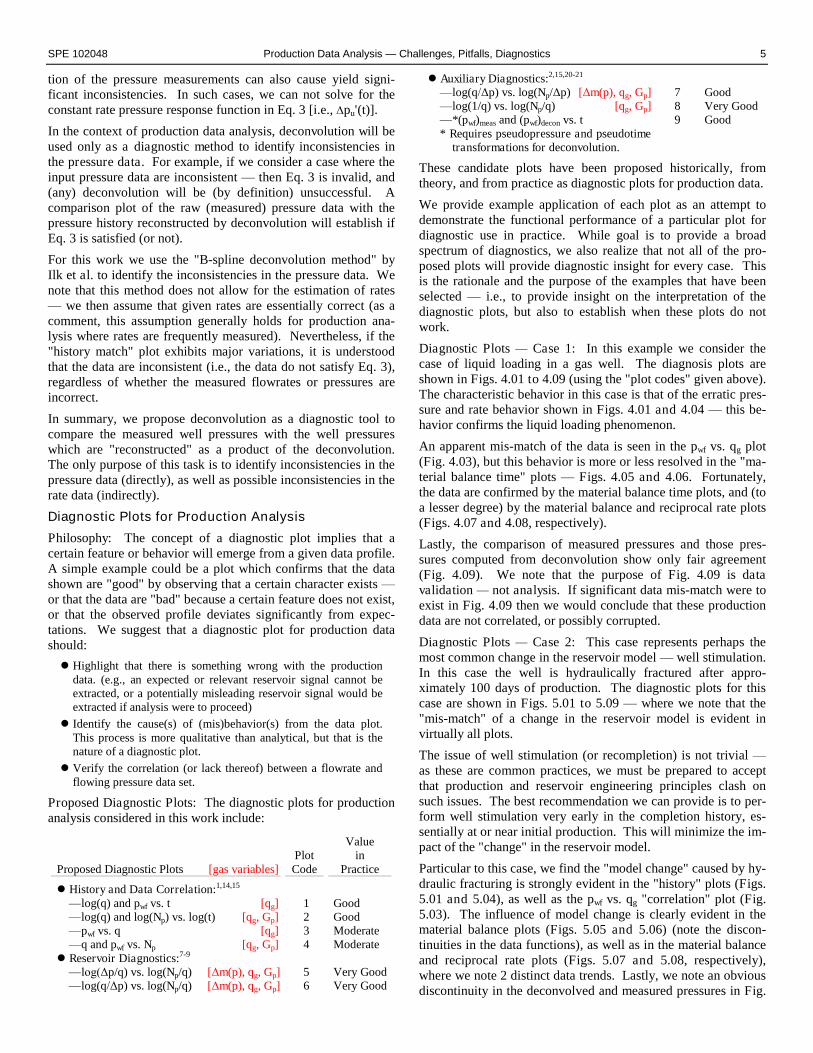
tion of the pressure measurements can also cause yield signi-ficant inconsistencies. In such cases, we can not solve for theconstant rate pressure response function in Eq. 3 [i.e., pu'(t)].

In the context of production data analysis, deconvolution will beused only as a diagnostic method to identify inconsistencies inthe pressure data. For example, if we consider a case where theinput pressure data are inconsistent — then Eq. 3 is invalid, and(any) deconvolution will be (by definition) unsuccessful. Acomparison plot of the raw (measured) pressure data with thepressure history reconstructed by deconvolution will establish ifEq. 3 is satisfied (or not).

For this work we use the "B-spline deconvolution method" byIlk et al. to identify the inconsistencies in the pressure data. Wenote that this method does not allow for the estimation of rates— we then assume that given rates are essentially correct (as acomment, this assumption generally holds for production ana-lysis where rates are frequently measured). Nevertheless, if the"history match" plot exhibits major variations, it is understoodthat the data are inconsistent (i.e., the data do not satisfy Eq. 3),regardless of whether the measured flowrates or pressures areincorrect.

In summary, we propose deconvolution as a diagnostic tool tocompare the measured well pressures with the well pressureswhich are "reconstructed" as a product of the deconvolution.The only purpose of this task is to identify inconsistencies in thepressure data (directly), as well as possible inconsistencies in therate data (indirectly).

Diagnostic Plots for Production Analysis

Philosophy: The concept of a diagnostic plot implies that acertain feature or behavior will emerge from a given data profile.A simple example could be a plot which confirms that the datashown are "good" by observing that a certain character exists —or that the data are "bad" because a certain feature does not exist,or that the observed profile deviates significantly from expec-tations. We suggest that a diagnostic plot for production datashould:

Highlight that there is something wrong with the productiondata. (e.g., an expected or relevant reservoir signal cannot beextracted, or a potentially misleading reservoir signal would beextracted if analysis were to proceed)

Identify the cause(s) of (mis)behavior(s) from the data plot.This process is more qualitative than analytical, but that is thenature of a diagnostic plot.

Verify the correlation (or lack thereof) between a flowrate andflowing pressure data set.

Proposed Diagnostic Plots: The diagnostic plots for productionanalysis considered in this work include:

Proposed Diagnostic Plots [gas variables]PlotCode

Valuein

Practice

History and Data Correlation:1,14,15

—log(q) and pwf vs. t [qg]—log(q) and log(Np) vs. log(t) [qg, Gp]—pwf vs. q [qg]—q and pwf vs. Np [qg, Gp]

1234

GoodGoodModerateModerate

Reservoir Diagnostics:7-9

—log(Δp/q) vs. log(Np/q) [Δm(p), qg, Gp]—log(q/Δp) vs. log(Np/q) [Δm(p), qg, Gp]

56

Very GoodVery Good

Auxiliary Diagnostics:2,15,20-21

—log(q/Δp) vs. log(Np/Δp) [Δm(p), qg, Gp]—log(1/q) vs. log(Np/q) [qg, Gp]—*(pwf)meas and (pwf)decon vs. t* Requires pseudopressure and pseudotime

transformations for deconvolution.

789

GoodVery GoodGood

These candidate plots have been proposed historically, fromtheory, and from practice as diagnostic plots for production data.

We provide example application of each plot as an attempt todemonstrate the functional performance of a particular plot fordiagnostic use in practice. While goal is to provide a broadspectrum of diagnostics, we also realize that not all of the pro-posed plots will provide diagnostic insight for every case. Thisis the rationale and the purpose of the examples that have beenselected — i.e., to provide insight on the interpretation of thediagnostic plots, but also to establish when these plots do notwork.

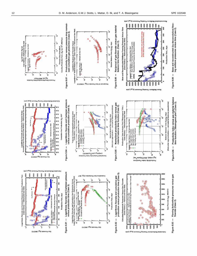
Diagnostic Plots — Case 1: In this example we consider thecase of liquid loading in a gas well. The diagnosis plots areshown in Figs. 4.01 to 4.09 (using the "plot codes" given above).The characteristic behavior in this case is that of the erratic pres-sure and rate behavior shown in Figs. 4.01 and 4.04 — this be-havior confirms the liquid loading phenomenon.

An apparent mis-match of the data is seen in the pwf vs. qg plot(Fig. 4.03), but this behavior is more or less resolved in the "ma-terial balance time" plots — Figs. 4.05 and 4.06. Fortunately,the data are confirmed by the material balance time plots, and (toa lesser degree) by the material balance and reciprocal rate plots(Figs. 4.07 and 4.08, respectively).

Lastly, the comparison of measured pressures and those pres-sures computed from deconvolution show only fair agreement(Fig. 4.09). We note that the purpose of Fig. 4.09 is datavalidation — not analysis. If significant data mis-match were toexist in Fig. 4.09 then we would conclude that these productiondata are not correlated, or possibly corrupted.

Diagnostic Plots — Case 2: This case represents perhaps themost common change in the reservoir model — well stimulation.In this case the well is hydraulically fractured after appro-ximately 100 days of production. The diagnostic plots for thiscase are shown in Figs. 5.01 to 5.09 — where we note that the"mis-match" of a change in the reservoir model is evident invirtually all plots.

The issue of well stimulation (or recompletion) is not trivial —as these are common practices, we must be prepared to acceptthat production and reservoir engineering principles clash onsuch issues. The best recommendation we can provide is to per-form well stimulation very early in the completion history, es-sentially at or near initial production. This will minimize the im-pact of the "change" in the reservoir model.

Particular to this case, we find the "model change" caused by hy-draulic fracturing is strongly evident in the "history" plots (Figs.5.01 and 5.04), as well as the pwf vs. qg "correlation" plot (Fig.5.03). The influence of model change is clearly evident in thematerial balance plots (Figs. 5.05 and 5.06) (note the discon-tinuities in the data functions), as well as in the material balanceand reciprocal rate plots (Figs. 5.07 and 5.08, respectively),where we note 2 distinct data trends. Lastly, we note an obviousdiscontinuity in the deconvolved and measured pressures in Fig.

6 D. M. Anderson, G.W.J. Stotts, L. Mattar, D. Ilk, and T. A. Blasingame SPE 102048

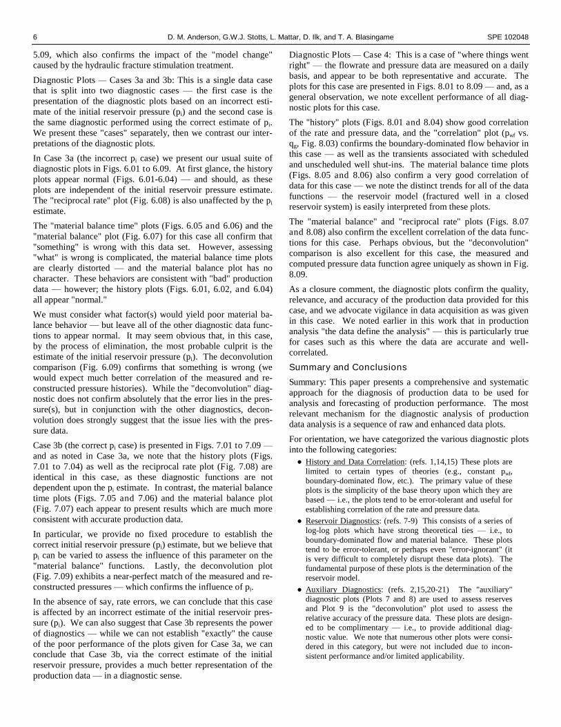
5.09, which also confirms the impact of the "model change"caused by the hydraulic fracture stimulation treatment.

Diagnostic Plots — Cases 3a and 3b: This is a single data casethat is split into two diagnostic cases — the first case is thepresentation of the diagnostic plots based on an incorrect esti-mate of the initial reservoir pressure (pi) and the second case isthe same diagnostic performed using the correct estimate of pi.We present these "cases" separately, then we contrast our inter-pretations of the diagnostic plots.

In Case 3a (the incorrect pi case) we present our usual suite ofdiagnostic plots in Figs. 6.01 to 6.09. At first glance, the historyplots appear normal (Figs. 6.01-6.04) — and should, as theseplots are independent of the initial reservoir pressure estimate.The "reciprocal rate" plot (Fig. 6.08) is also unaffected by the pi

estimate.

The "material balance time" plots (Figs. 6.05 and 6.06) and the"material balance" plot (Fig. 6.07) for this case all confirm that"something" is wrong with this data set. However, assessing"what" is wrong is complicated, the material balance time plotsare clearly distorted — and the material balance plot has nocharacter. These behaviors are consistent with "bad" productiondata — however; the history plots (Figs. 6.01, 6.02, and 6.04)all appear "normal."

We must consider what factor(s) would yield poor material ba-lance behavior — but leave all of the other diagnostic data func-tions to appear normal. It may seem obvious that, in this case,by the process of elimination, the most probable culprit is theestimate of the initial reservoir pressure (pi). The deconvolutioncomparison (Fig. 6.09) confirms that something is wrong (wewould expect much better correlation of the measured and re-constructed pressure histories). While the "deconvolution" diag-nostic does not confirm absolutely that the error lies in the pres-sure(s), but in conjunction with the other diagnostics, decon-volution does strongly suggest that the issue lies with the pres-sure data.

Case 3b (the correct pi case) is presented in Figs. 7.01 to 7.09 —and as noted in Case 3a, we note that the history plots (Figs.7.01 to 7.04) as well as the reciprocal rate plot (Fig. 7.08) areidentical in this case, as these diagnostic functions are notdependent upon the pi estimate. In contrast, the material balancetime plots (Figs. 7.05 and 7.06) and the material balance plot(Fig. 7.07) each appear to present results which are much moreconsistent with accurate production data.

In particular, we provide no fixed procedure to establish thecorrect initial reservoir pressure (pi) estimate, but we believe thatpi can be varied to assess the influence of this parameter on the"material balance" functions. Lastly, the deconvolution plot(Fig. 7.09) exhibits a near-perfect match of the measured and re-constructed pressures — which confirms the influence of pi.

In the absence of say, rate errors, we can conclude that this caseis affected by an incorrect estimate of the initial reservoir pres-sure (pi). We can also suggest that Case 3b represents the powerof diagnostics — while we can not establish "exactly" the causeof the poor performance of the plots given for Case 3a, we canconclude that Case 3b, via the correct estimate of the initialreservoir pressure, provides a much better representation of theproduction data — in a diagnostic sense.

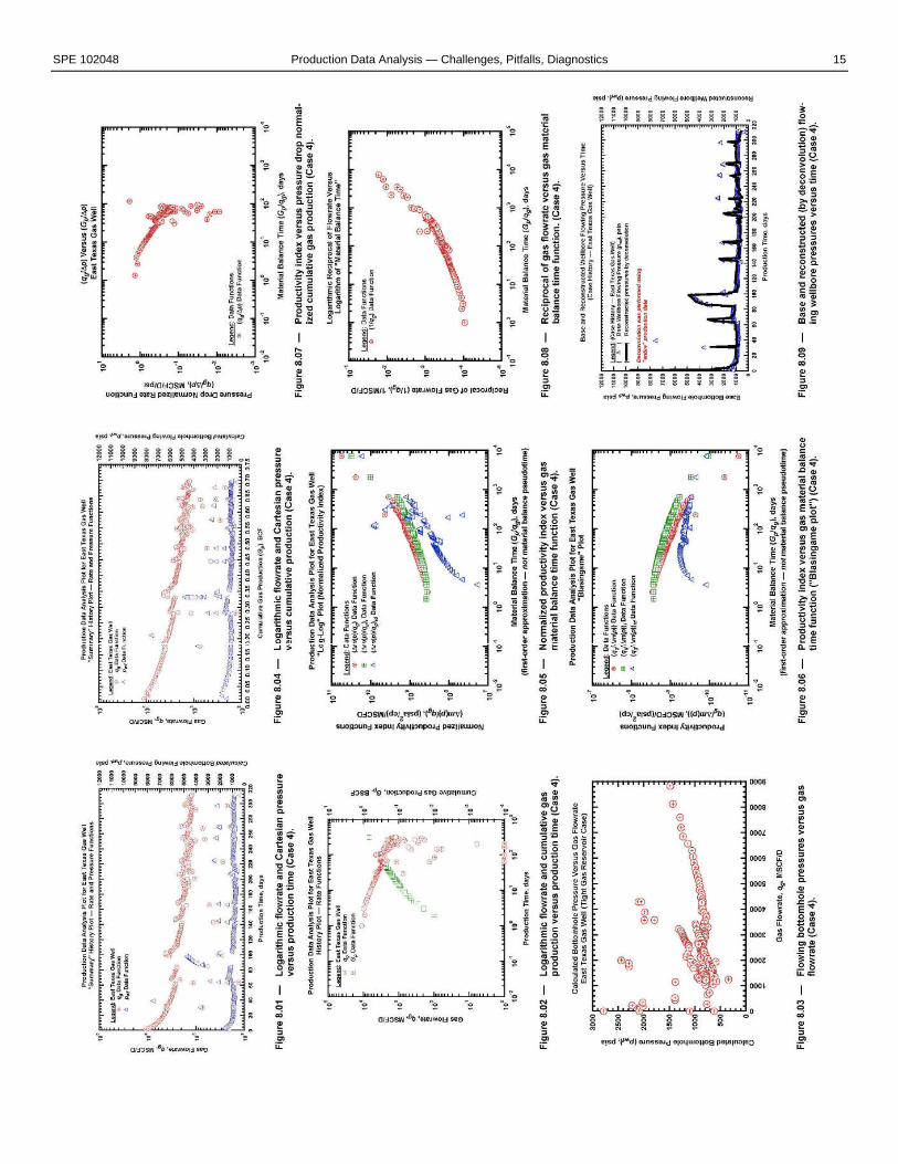
Diagnostic Plots —Case 4: This is a case of "where things wentright" — the flowrate and pressure data are measured on a dailybasis, and appear to be both representative and accurate. Theplots for this case are presented in Figs. 8.01 to 8.09 — and, as ageneral observation, we note excellent performance of all diag-nostic plots for this case.

The "history" plots (Figs. 8.01 and 8.04) show good correlationof the rate and pressure data, and the "correlation" plot (pwf vs.qg, Fig. 8.03) confirms the boundary-dominated flow behavior inthis case — as well as the transients associated with scheduledand unscheduled well shut-ins. The material balance time plots(Figs. 8.05 and 8.06) also confirm a very good correlation ofdata for this case — we note the distinct trends for all of the datafunctions — the reservoir model (fractured well in a closedreservoir system) is easily interpreted from these plots.

The "material balance" and "reciprocal rate" plots (Figs. 8.07and 8.08) also confirm the excellent correlation of the data func-tions for this case. Perhaps obvious, but the "deconvolution"comparison is also excellent for this case, the measured andcomputed pressure data function agree uniquely as shown in Fig.8.09.

As a closure comment, the diagnostic plots confirm the quality,relevance, and accuracy of the production data provided for thiscase, and we advocate vigilance in data acquisition as was givenin this case. We noted earlier in this work that in productionanalysis "the data define the analysis" — this is particularly truefor cases such as this where the data are accurate and well-correlated.

Summary and Conclusions

Summary: This paper presents a comprehensive and systematicapproach for the diagnosis of production data to be used foranalysis and forecasting of production performance. The mostrelevant mechanism for the diagnostic analysis of productiondata analysis is a sequence of raw and enhanced data plots.

For orientation, we have categorized the various diagnostic plotsinto the following categories:●History and Data Correlation: (refs. 1,14,15) These plots are

limited to certain types of theories (e.g., constant pwf,boundary-dominated flow, etc.). The primary value of theseplots is the simplicity of the base theory upon which they arebased — i.e., the plots tend to be error-tolerant and useful forestablishing correlation of the rate and pressure data.

●Reservoir Diagnostics: (refs. 7-9) This consists of a series oflog-log plots which have strong theoretical ties — i.e., toboundary-dominated flow and material balance. These plotstend to be error-tolerant, or perhaps even "error-ignorant" (itis very difficult to completely disrupt these data plots). Thefundamental purpose of these plots is the determination of thereservoir model.

●Auxiliary Diagnostics: (refs. 2,15,20-21) The "auxiliary"diagnostic plots (Plots 7 and 8) are used to assess reservesand Plot 9 is the "deconvolution" plot used to assess therelative accuracy of the pressure data. These plots are design-ed to be complimentary — i.e., to provide additional diag-nostic value. We note that numerous other plots were consi-dered in this category, but were not included due to incon-sistent performance and/or limited applicability.

SPE 102048 Production Data Analysis — Challenges, Pitfalls, Diagnostics 7

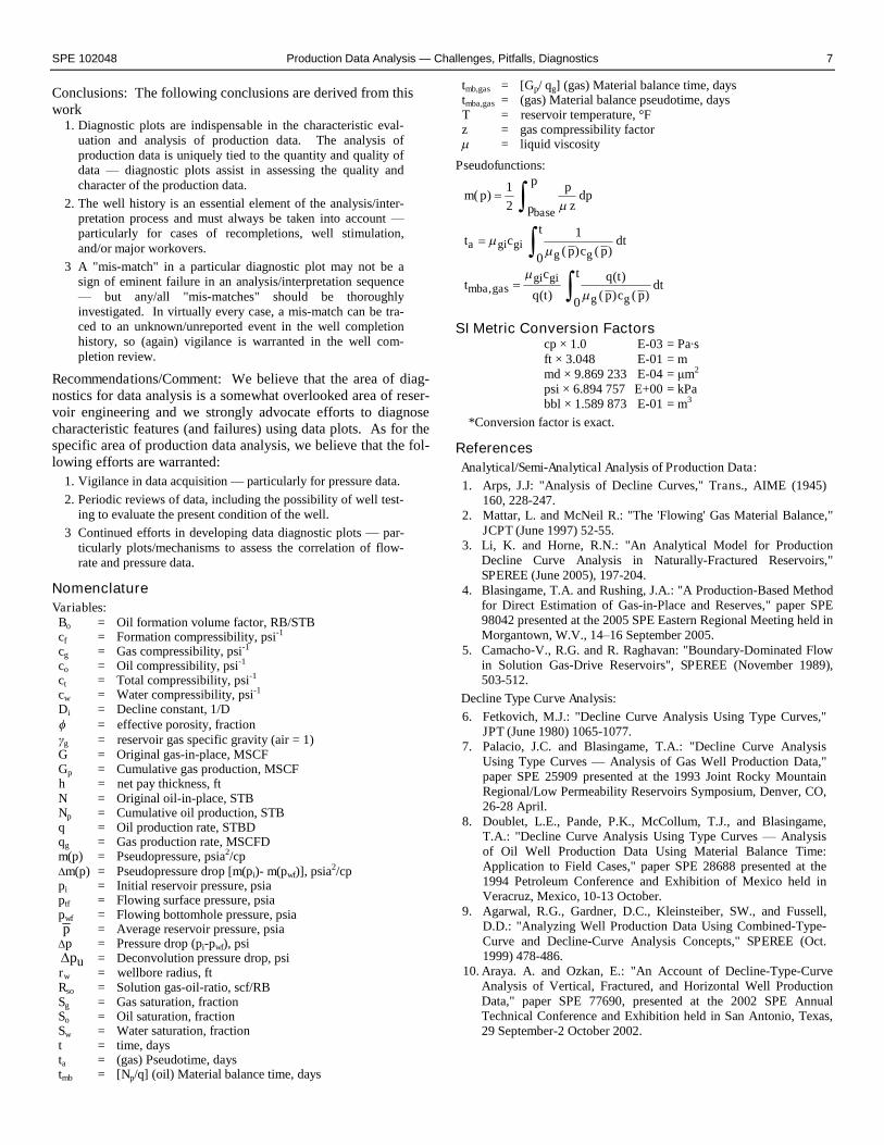
Conclusions: The following conclusions are derived from thiswork

1. Diagnostic plots are indispensable in the characteristic eval-uation and analysis of production data. The analysis ofproduction data is uniquely tied to the quantity and quality ofdata — diagnostic plots assist in assessing the quality andcharacter of the production data.

2. The well history is an essential element of the analysis/inter-pretation process and must always be taken into account —particularly for cases of recompletions, well stimulation,and/or major workovers.

3 A "mis-match" in a particular diagnostic plot may not be asign of eminent failure in an analysis/interpretation sequence— but any/all "mis-matches" should be thoroughlyinvestigated. In virtually every case, a mis-match can be tra-ced to an unknown/unreported event in the well completionhistory, so (again) vigilance is warranted in the well com-pletion review.

Recommendations/Comment: We believe that the area of diag-nostics for data analysis is a somewhat overlooked area of reser-voir engineering and we strongly advocate efforts to diagnosecharacteristic features (and failures) using data plots. As for thespecific area of production data analysis, we believe that the fol-lowing efforts are warranted:

1. Vigilance in data acquisition — particularly for pressure data.2. Periodic reviews of data, including the possibility of well test-

ing to evaluate the present condition of the well.3 Continued efforts in developing data diagnostic plots — par-

ticularly plots/mechanisms to assess the correlation of flow-rate and pressure data.

NomenclatureVariables:Bo = Oil formation volume factor, RB/STBcf = Formation compressibility, psi-1

cg = Gas compressibility, psi-1

co = Oil compressibility, psi-1

ct = Total compressibility, psi-1

cw = Water compressibility, psi-1

Di = Decline constant, 1/D = effective porosity, fractionγg = reservoir gas specific gravity (air = 1)G = Original gas-in-place, MSCFGp = Cumulative gas production, MSCFh = net pay thickness, ftN = Original oil-in-place, STBNp = Cumulative oil production, STBq = Oil production rate, STBDqg = Gas production rate, MSCFDm(p) = Pseudopressure, psia2/cpm(p) = Pseudopressure drop [m(pi)- m(pwf)], psia2/cppi = Initial reservoir pressure, psiaptf = Flowing surface pressure, psiapwf = Flowing bottomhole pressure, psiap = Average reservoir pressure, psiap = Pressure drop (pi-pwf), psi

up = Deconvolution pressure drop, psirw = wellbore radius, ftRso = Solution gas-oil-ratio, scf/RBSg = Gas saturation, fractionSo = Oil saturation, fractionSw = Water saturation, fractiont = time, daysta = (gas) Pseudotime, daystmb = [Np/q] (oil) Material balance time, days

tmb,gas = [Gp/ qg] (gas) Material balance time, daystmba,gas = (gas) Material balance pseudotime, daysT = reservoir temperature, °Fz = gas compressibility factor = liquid viscosity

Pseudofunctions:

dpz

pp

ppm

base21

)(

dtpcp

tct

gggigia )()(

1

0

dtpcp

tqt

tq

ct

gg

gigigasmba )()(

)(

0)(,

SI Metric Conversion Factorscp × 1.0 E-03 = Pa∙sft × 3.048 E-01 = mmd × 9.869 233 E-04 = μm2

psi × 6.894 757 E+00 = kPabbl × 1.589 873 E-01 = m3

*Conversion factor is exact.

ReferencesAnalytical/Semi-Analytical Analysis of Production Data:1. Arps, J.J: "Analysis of Decline Curves," Trans., AIME (1945)

160, 228-247.2. Mattar, L. and McNeil R.: "The 'Flowing' Gas Material Balance,"

JCPT (June 1997) 52-55.3. Li, K. and Horne, R.N.: "An Analytical Model for Production

Decline Curve Analysis in Naturally-Fractured Reservoirs,"SPEREE (June 2005), 197-204.

4. Blasingame, T.A. and Rushing, J.A.: "A Production-Based Methodfor Direct Estimation of Gas-in-Place and Reserves," paper SPE98042 presented at the 2005 SPE Eastern Regional Meeting held inMorgantown, W.V., 14–16 September 2005.

5. Camacho-V., R.G. and R. Raghavan: "Boundary-Dominated Flowin Solution Gas-Drive Reservoirs", SPEREE (November 1989),503-512.

Decline Type Curve Analysis:6. Fetkovich, M.J.: "Decline Curve Analysis Using Type Curves,"

JPT (June 1980) 1065-1077.7. Palacio, J.C. and Blasingame, T.A.: "Decline Curve Analysis

Using Type Curves — Analysis of Gas Well Production Data,"paper SPE 25909 presented at the 1993 Joint Rocky MountainRegional/Low Permeability Reservoirs Symposium, Denver, CO,26-28 April.

8. Doublet, L.E., Pande, P.K., McCollum, T.J., and Blasingame,T.A.: "Decline Curve Analysis Using Type Curves — Analysisof Oil Well Production Data Using Material Balance Time:Application to Field Cases," paper SPE 28688 presented at the1994 Petroleum Conference and Exhibition of Mexico held inVeracruz, Mexico, 10-13 October.

9. Agarwal, R.G., Gardner, D.C., Kleinsteiber, SW., and Fussell,D.D.: "Analyzing Well Production Data Using Combined-Type-Curve and Decline-Curve Analysis Concepts," SPEREE (Oct.1999) 478-486.

10. Araya. A. and Ozkan, E.: "An Account of Decline-Type-CurveAnalysis of Vertical, Fractured, and Horizontal Well ProductionData," paper SPE 77690, presented at the 2002 SPE AnnualTechnical Conference and Exhibition held in San Antonio, Texas,29 September-2 October 2002.

8 D. M. Anderson, G.W.J. Stotts, L. Mattar, D. Ilk, and T. A. Blasingame SPE 102048

11. Fuentes-C., G., Camacho-V., R.G., Vásquez-C., M.: "PressureTransient and Decline Curve Behaviors for Partially PenetratingWells Completed in Naturally Fractured-Vuggy Reservoirs," paperSPE 92116 presented at the 2004 SPE International PetroleumConference in Mexico, Puebla, Mexico, 8–9 November, 2004.

Diagnostic Methods for Production Data Analysis:12. Mattar, L. and Anderson, D.: "A systematic and Comprehensive

Methodology for Advanced Analysis of Production Data," paperSPE 84472 presented at the 2003 SPE Technical Conference andExhibition, Denver, Oct. 5-8.

13. Anderson, D. and Mattar, L.: "Practical Diagnostics Using Pro-duction Data and Flowing Pressures," paper SPE 89939 presentedat the 2004 Annual SPE Technical Conference and Exhibition,Houston, TX., 26-29 September 2004.

14. Kabir, CS. and Izgec, B.: "Diagnosis of Reservoir Behavior fromMeasured Pressure/Rate Data," paper SPE 100384 presented at the2006 SPE Gas Technology Symposium held in Calgary, Alberta,Canada, 15–17 May 2006.

15. Bondar, V.V.: The Analysis of Water-Oil Ratio (WOR) Behavior inReservoir System, MS Thesis, Texas A&M U. College Station, TX(May 2001).

Deconvolution:16. von Schroeter, T., Hollaender, F., and Gringarten, A.C.:

"Analysis of Well Test Data From Downhole PermanentDownhole Gauges by Deconvolution," paper SPE 77688presented at the 2002 SPE Annual Technical Conference andExhibition, San Antonio, Texas, 29 Spetember-2 October.

17. von Schroeter, T., Hollaender, F., and Gringarten, A.C.: "Decon-volution of Well Test Data as a Nonlinear Total Least SquaresProblem," SPEJ (December 2004) 375.

18. Levitan, M.M.: "Practical Application of Pressure/Rate Decon-volution to Analysis of Real Well Tests," SPEREE (April 2005)113.

19. Levitan, M.M., Crawford, G.E., and Hardwick, A., "Practical Con-siderations for Pressure-Rate Deconvolution of Well-Test Data,"SPEJ (March 2006) 35.

20. Ilk, D., Valko, P.P., and Blasingame, T.A.: "Deconvolution ofVariable-Rate Reservoir Performance Data Using B-Splines,"paper SPE 95571 presented at the 2005 SPE Annual TechnicalConference and Exhibition, Dallas, TX, 9-12 October.

21. Ilk, D., Anderson, D.M., Valko, P.P., and Blasingame, T.A.:"Analysis of Gas Well Reservoir Performance Data Using B-Spline Deconvolution," paper SPE 100573 presented at the 2006SPE Gas Technology Symposium, Calgary, Alberta, Canada, 15-17 May.

22. Kuchuk, F.J., Hollaender, F., Gok, I.M., and Onur, M.: "DeclineCurves from Deconvolution of Pressure and Flow-Rate Measure-ments for Production Optimization and Prediction," paper SPE96002 presented at the 2005 SPE Annual Technical Conferenceand Exhibition, Dallas, TX, 9-12 October.

SPE 102048 Production Data Analysis — Challenges, Pitfalls, Diagnostics 9

Unfractured Well (Radial Flow)Fractured Well (Infinite Fracture Conductivity)Fractured Well (Finite Fracture Conductivity)Horizontal Well (Full Penetration — Thick Reservoir)Horizontal Well (Full Penetration — Thin Reservoir)

Transient Flow Region(Estimation of

Reservoir PROPERTIES)

Fractured Well ina Bounded Circular

Reservoir(Infinite Conductivity

Vertical Fracture)

Schematic Pressure Integral-Derivative Function — Material Balance Time FormatVarious Reservoir Models and Well Configurations (as noted)

DIAGNOSTIC plot for Production Data (Rate-Normalized Pressure Drop Functions)

Pre

ssu

reIn

teg

ral-

Der

ivat

ive

Fu

nct

ion

inT

erm

so

fM

ater

ialB

alan

ceT

Ime

Unfractured Well ina Bounded Circular

Reservoir

Fractured Well ina Bounded Circular

Reservoir(Finite ConductivityVertical Fracture)

2

1

1

4

1

1

Boundary-DominatedFlow Region(Estimation of

Reservoir VOLUME)

Horizontal Well in aBounded Square

Reservoir

ThinReservoir

ThickReservoir

( )

( ) ( )

( )

( )

1

2

2

1

Material Balance TIme Function

Figure 1 — Schematic/diagnostic plot for production data analysis (rate-normalized pressure drop integral-derivative function — material balance time format). This format provides a "well test" equivalentbehavior, increasing pressure functions with time.

Unfractured Well (Radial Flow)Fractured Well (Infinite Fracture Conductivity)Fractured Well (Finite Fracture Conductivity)Horizontal Well (Full Penetration — Thick Reservoir)Horizontal Well (Full Penetration — Thin Reservoir)

Transient Flow Region(Estimation of

Reservoir PROPERTIES)

Fractured Well ina Bounded Circular

Reservoir(Infinite Conductivity

Vertical Fracture)

Schematic Rate Integral-Derivative Function — Material Balance Time FormatVarious Reservoir Models and Well Configurations (as noted)

DIAGNOSTIC plot for Production Data (Pressure Drop-Normalized Rate Functions)

Rat

eIn

teg

ral-

Der

ivat

ive

Fu

nct

ion

inT

erm

so

fM

ater

ialB

alan

ceT

Ime

Unfractured Well ina Bounded Circular

Reservoir

Fractured Well ina Bounded Circular

Reservoir(Finite Conductivity

Vertical Fracture)2

11

4

1

1

Boundary-DominatedFlow Region(Estimation of

Reservoir VOLUME)

ThinReservoir

ThickReservoir

( )

( ) ( )

( )

( )

Horizontal Well in aBounded Square

Reservoir

Horizontal well:Early transientradial flow behavior. Horizontal well:

Transient linear flow behavior,does not develop linear trends(e.g., -1/2) due to earlier regimes.

Material Balance TIme Function

Figure 2 — Schematic/diagnostic plot for production data analysis (pressure drop-normalized rate integral-derivative function — material balance time format). This format provides a "decline type curve"equivalent behavior, decreasing rate functions with time.

10 D. M. Anderson, G.W.J. Stotts, L. Mattar, D. Ilk, and T. A. Blasingame SPE 102048

Figure 3 — Guidelines for production analysis. Emphasis is placed on the diagnostic analysis — establishing thequality and correlation of the production rates and pressures; then establishing the reservoir modelusing characteristic (log-log) plots.

SPE 102048 Production Data Analysis — Challenges, Pitfalls, Diagnostics 11

12 D. M. Anderson, G.W.J. Stotts, L. Mattar, D. Ilk, and T. A. Blasingame SPE 102048

SPE 102048 Production Data Analysis — Challenges, Pitfalls, Diagnostics 13

14 D. M. Anderson, G.W.J. Stotts, L. Mattar, D. Ilk, and T. A. Blasingame SPE 102048

SPE 102048 Production Data Analysis — Challenges, Pitfalls, Diagnostics 15