Spatiotemporal Patterns in Ecology and Epidemiology
210
Spatiotemporal Patterns in Ecology and Epidemiology Theory, Models, and Simulation C6749_FM.indd 1 11/13/07 2:17:40 PM
Transcript of Spatiotemporal Patterns in Ecology and Epidemiology

Spatiotemporal Patterns in
Ecology and EpidemiologyTheory, Models, and Simulation
C6749_FM.indd 1 11/13/07 2:17:40 PM

CHAPMAN & HALL/CRCMathematical and Computational Biology Series
Aims and scope:This series aims to capture new developments and summarize what is known over the wholespectrum of mathematical and computational biology and medicine. It seeks to encourage theintegration of mathematical, statistical and computational methods into biology by publishinga broad range of textbooks, reference works and handbooks. The titles included in the series aremeant to appeal to students, researchers and professionals in the mathematical, statistical andcomputational sciences, fundamental biology and bioengineering, as well as interdisciplinaryresearchers involved in the field. The inclusion of concrete examples and applications, andprogramming techniques and examples, is highly encouraged.
Series EditorsAlison M. EtheridgeDepartment of StatisticsUniversity of Oxford
Louis J. GrossDepartment of Ecology and Evolutionary BiologyUniversity of Tennessee
Suzanne LenhartDepartment of MathematicsUniversity of Tennessee
Philip K. MainiMathematical InstituteUniversity of Oxford
Shoba RanganathanResearch Institute of BiotechnologyMacquarie University
Hershel M. SaferWeizmann Institute of ScienceBioinformatics & Bio Computing
Eberhard O. VoitThe Wallace H. Couter Department of Biomedical EngineeringGeorgia Tech and Emory University
Proposals for the series should be submitted to one of the series editors above or directly to:CRC Press, Taylor & Francis GroupAlbert House, 4th floor1-4 Singer StreetLondon EC2A 4BQUK
C6749_FM.indd 2 11/13/07 2:17:40 PM

Published Titles
Bioinformatics: A Practical ApproachShui Qing Ye
Cancer Modelling and SimulationLuigi Preziosi
Computational Biology: A Statistical Mechanics PerspectiveRalf Blossey
Computational Neuroscience: A Comprehensive ApproachJianfeng Feng
Data Analysis Tools for DNA MicroarraysSorin Draghici
Differential Equations and Mathematical BiologyD.S. Jones and B.D. Sleeman
Exactly Solvable Models of Biological InvasionSergei V. Petrovskii and Bai-Lian Li
Introduction to BioinformaticsAnna Tramontano
An Introduction to Systems Biology: Design Principles of Biological CircuitsUri Alon
Knowledge Discovery in ProteomicsIgor Jurisica and Dennis Wigle
Modeling and Simulation of Capsules and Biological CellsC. Pozrikidis
Niche Modeling: Predictions from Statistical DistributionsDavid Stockwell
Normal Mode Analysis: Theory and Applications to Biological andChemical SystemsQiang Cui and Ivet Bahar
Pattern Discovery in Bioinformatics: Theory & AlgorithmsLaxmi Parida
Spatiotemporal Patterns in Ecology and Epidemiology: Theory, Models, and SimulationHorst Malchow, Sergei V. Petrovskii, and Ezio Venturino
Stochastic Modelling for Systems BiologyDarren J. Wilkinson
The Ten Most Wanted Solutions in Protein BioinformaticsAnna Tramontano
C6749_FM.indd 3 11/13/07 2:17:40 PM

C6749_FM.indd 4 11/13/07 2:17:40 PM

Horst Malchow, Sergei V. Petrovskii,
and Ezio Venturino
Spatiotemporal Patterns in
Ecology and EpidemiologyTheory, Models, and Simulation
C6749_FM.indd 5 11/13/07 2:17:41 PM

Chapman & Hall/CRCTaylor & Francis Group6000 Broken Sound Parkway NW, Suite 300Boca Raton, FL 33487‑2742
© 2008 by Taylor & Francis Group, LLC Chapman & Hall/CRC is an imprint of Taylor & Francis Group, an Informa business
No claim to original U.S. Government worksPrinted in the United States of America on acid‑free paper10 9 8 7 6 5 4 3 2 1
International Standard Book Number‑13: 978‑1‑58488‑674‑7 (Hardcover)
This book contains information obtained from authentic and highly regarded sources. Reprinted material is quoted with permission, and sources are indicated. A wide variety of references are listed. Reasonable efforts have been made to publish reliable data and information, but the author and the publisher cannot assume responsibility for the validity of all materials or for the conse‑quences of their use.
Except as permitted under U.S. Copyright Law, no part of this book may be reprinted, reproduced, transmitted, or utilized in any form by any electronic, mechanical, or other means, now known or hereafter invented, including photocopying, microfilming, and recording, or in any information storage or retrieval system, without written permission from the publishers.
For permission to photocopy or use material electronically from this work, please access www.copyright.com (http://www.copyright.com/) or contact the Copyright Clearance Center, Inc. (CCC) 222 Rosewood Drive, Danvers, MA 01923, 978‑750‑8400. CCC is a not‑for‑profit organization that provides licenses and registration for a variety of users. For organizations that have been granted a photocopy license by the CCC, a separate system of payment has been arranged.
Trademark Notice: Product or corporate names may be trademarks or registered trademarks, and are used only for identification and explanation without intent to infringe.
Library of Congress Cataloging‑in‑Publication Data
Malchow, Horst, 1953‑Spatiotemporal patterns in ecology and epidemiology : theory, models, and
simulation / Horst Malchow, Sergei V Petrovskii and Ezio Venturino.p. cm. ‑‑ (Chapman & Hall/CRC mathematical and computational biology ; 17)
Includes bibliographical references and index.ISBN 978‑1‑58488‑674‑7 (alk. paper)1. Ecology‑‑Mathematical models. 2. Epidemiology‑‑Mathematical models. I.
Petrovskii, Sergei V. II. Venturino, Ezio. III. Title. III. Series.
QH541.15.M3M25 2008577.01’5118‑‑dc22 2007040410
Visit the Taylor & Francis Web site athttp://www.taylorandfrancis.com
and the CRC Press Web site athttp://www.crcpress.com
C6749_FM.indd 6 11/13/07 2:17:41 PM

Preface
Dynamics has always been a core issue of all natural sciences. What arethe driving forces and the “mechanisms” that result in motion of the systemparts and/or lead to its evolution as a whole, whatever that system maybe (particular cases range from a single rigid body to the human society)?What are the properties and scenarios of this motion and evolution? Whatcan be the meaning or implication of this dynamics if considered in a widercontext, e.g., through interaction with other systems or other sciences? Thesehave been challenging and exciting problems for philosophers and scientiststhroughout at least 30 centuries.
The focus of interest has evolved, too. At the dawn of contemporary science,stationary processes were regarded as the essence of dynamics. Non-stationarymotion was often either attributed to a specific cause (such as periodic forcing)or considered as a mere transient that was bound to die out after a relativelyshort relaxation time. The corresponding system’s geometry was assumed tobe smooth and regular. Those phenomena that did not fit into this philosophy,turbulent flow being the renowned example, were regarded as exotic and rareand, possibly, not self-sustained.
Although this mainstream thought of science has been challenged from timeto time from as early as ancient Greece, it was not until the late twentiethcentury that it was widely realized that the dynamics of even very simple sys-tems can be – and often is – completely different and much more complicated.Relaxation to steady states and periodic motion (with the limit cycle as itsmathematical paradigm), which used to be the main elements of dynamics,were displaced by the concept of deterministic chaos. Smooth surfaces andsimple curves gave way to objects with fractal properties. Moreover, chaos andfractals were eventually found (if not empirically, then at least theoretically)nearly everywhere, from lasers to animal behavior.
Even more importantly, it was realized that complex temporal dynamicsand, especially, spatial structures do not just exist per se but can arise asa result of a system’s self-organization. In an open system, i.e., a systemwith an inflow of mass and/or energy, the dynamics can become intrinsicallyunstable, resulting either in the formation of periodic spatial patterns or in acomplicated turbulence-like spatiotemporal behaviour.
A similar evolution of concepts and ideas occurred in ecology and popu-lation biology. Ecologists have long been aware that population distributionin a natural environment is normally distinctly heterogeneous; however, thatwas usually regarded as a separate phenomenon that was not directly related
to the main properties of population dynamics in time such as its persis-tence, reproductive success, etc. Correspondingly, earlier studies tended tofocus mainly on the dynamics of “nonspatial” systems (i.e., systems wherethe spatial distribution of all factors and agents was regarded to be homoge-neous under any circumstances). The results of the last two decades, however,proved that the impact of spatial dimensions can be crucial. The dynamicsof a spatially extended system can be qualitatively different from the dynam-ics of its nonspatial counterpart due to self-organized, “spontaneous” patternformation.
It should be mentioned that recent progress in theoretical ecology would un-likely have become possible without extensive use of mathematical modeling.There are several reasons why a complete and thorough study of ecosystemdynamics is hardly possible if based only on field data collection. Field obser-vations are often very expensive and field experiments can sometimes be dan-gerous for the environment. Moreover, a regular experimental study impliesreplicated experiments; however, this is hardly possible in ecology because ofthe virtual impossibility of reproducing the same initial and environmentalconditions. Note that mathematical models have been used in ecology fromas early as the nineteenth century (cf. the work by Malthus) but they becamea really powerful research tool after the development of numerical simulationapproaches and modern computers.
Importantly, although the spatial dimension of ecosystems dynamics isnowadays widely recognized, the specific mechanisms behind species pattern-ing in space are still poorly understood and the corresponding theoreticalframework is underdeveloped. In particular, existing textbooks and researchmonographs on theoretical/mathematical ecology, when addressing its spatialaspect, practically never go beyond the classical Turing scenario of patternformation. This book is designed to fill this gap, in particular, by givingan account of the significant progress made recently (and published in peri-odic scientific literature) in understanding these issues through mathematicalmodeling and numerical simulations using some basic, conceptual models ofpopulation dynamics.
A special remark should be made regarding terminology. Apparently, theterm “pattern” has originally appeared in application to spatial processeswhere some kind of heterogeneity is observed. In the context of this book,however, we use this term somewhat more broadly, embracing also the purelytemporal dynamics of spatially homogeneous systems; cf. “patterns of tempo-ral behaviour.”
Another tendency in scientific periodics over the last decade has been con-vergence between ecology and epidemiology. Although it seems to be commonknowledge that a disease can change population dynamics essentially, mathe-matical approaches to these issues remained distinctly different until recently.Remarkably, both population dynamics and disease dynamics exhibit manysimilar properties, especially with regards to pattern formation in space andtime. This book provides a first attempt at a unified approach to popula-

tion dynamics and epidemiology by means of considering a few “ecoepidemi-ological” models where both the basic interspecies interactions of populationdynamics and the impact of an infectious disease are considered explicitly.
The book is organized as follows. Part I starts with a general overview ofrelevant phenomena in ecology and epidemiology, giving also a few examplesof pattern formation in natural systems, and then proceeds to a brief synopsisof existing modeling approaches.
Part II deals with nonspatial models of population dynamics and epidemi-ology. We have already mentioned that the dynamics of spatial and corre-sponding nonspatial systems can be essentially different and the results ofnonspatial analysis may, in some cases, be misleading. Nevertheless, it is alsoclear that the properties of nonspatial dynamics provide a certain “skeleton”important for a thorough understanding of spatiotemporal dynamics. Corre-spondingly, Part II gives a wide panorama of existing nonspatial approaches,starting from basic ideas and elementary models and eventually bringing thereader to the state-of-the-art in this area.
In Part III, we introduce space by means of including “diffusion” of theindividuals and consider the main scenarios of spatial and spatiotemporalpattern formation in deterministic models of population dynamics.
Finally, in Part IV, we address the issue of interaction between deterministicand stochastic processes in ecosystem/epidemics dynamics and consider hownoise and stochasticity may affect pattern formation.
When writing this book, we were primarily thinking about experienced re-searchers in theoretical and mathematical ecology and/or in relevant areas ofapplied mathematics as the “target audience,” and that affected its structureand style. In particular, from the beginning of Part I we use some advancedterminology from applied dynamical systems, mathematical modelling, anddifferential equations, which requires the reader to have at least some basiceducation in these topics (even in spite of the fact that much of that termi-nology is actually explained later in the text). However, we do hope thatmany researchers from neighboring fields and also postgraduate students willfind this book useful as well; in order to encourage them to read it, we giveenough calculation details. For the same purpose, the presentation of someintroductory items is, at times, made on a rather elementary level.
A considerable part of the results included into this book was obtained innumerical simulations. Therefore, although numerical results by no meanscan be regarded as an adequate substitute to rigorous analysis, we thinkthat it will be only fair if the reader is given an opportunity to reproducethe main results and (which is probably even more important) to make adeeper look into the system’s dynamics in his/her own numerical experiments.For that purpose, a CD is attached to this book that contains many of thecomputer programs that we have used in our work. The programs are writtenin MATLAB; it must be mentioned here that MATLAB R© and Simulink R© aretrademarks of The MathWorks, Inc., and are used with permission. TheMathWorks does not warrant the accuracy of the programs on the CD. This

CD’s use or discussion of MATLAB R© and Simulink R© software or relatedproducts does not constitute endorsement or sponsorship by The MathWorksof a particular pedagogical approach or particular use of MATLAB R© andSimulink R© software.
In conclusion, it is our pleasure to express our gratitude to numerous peoplewho helped this book to appear through many fruitful discussions and helpfulcomments, both during manuscript preparation and during the equally impor-tant time preceding this work. We are particularly grateful to Ulrike Feudel,Nanako Shigesada, Michel Langlais, Michael Tretyakov, Lutz Schimansky-Geier, Vitaly Volpert, Andrey Morozov, Frank Hilker, Jean-Christophe Pog-giale, Hiromi Seno, Bai-Lian (Larry) Li, Herbert Hethcote, Alexander Medvin-sky, Joydev Chattopadhyay, Olivier Lejeune, Michael Sieber, Guido Badino,Francesca Bona, and Marco Isaia. S.P. is very thankful to his colleagues inthe Department of Mathematics of the University of Leicester for their con-tinuing encouragement and support. E.V. thanks the Max–Planck–Institutfur Mathematik in Bonn, where, during an informal visit, parts of this bookwere written. E.V. is also very much indebted to the persons who long ago in-troduced him to the fascinating field of mathematical modeling, especially toBrian Conolly, Edward Beltrami, and James Frauenthal. Last but not least,we all are thankful to Sunil Nair, publisher of mathematics and statistics,CRC Press/Chapman & Hall, for inviting us to write this book and for hispatience and encouragement.
H. Malchow, S. Petrovskii, E. VenturinoOsnabruck–Leicester/Birmingham–Torino

Contents
I Introduction 1
1 Ecological patterns in time and space 31.1 Local structures . . . . . . . . . . . . . . . . . . . . . . . . . 31.2 Spatial and spatiotemporal structures . . . . . . . . . . . . . 6
2 An overview of modeling approaches 11
II Models of temporal dynamics 19
3 Classical one population models 213.1 Isolated populations models . . . . . . . . . . . . . . . . . . 21
3.1.1 Scaling . . . . . . . . . . . . . . . . . . . . . . . . . . 253.2 Migration models . . . . . . . . . . . . . . . . . . . . . . . . 27
3.2.1 Harvesting . . . . . . . . . . . . . . . . . . . . . . . . 303.3 Glance at discrete models . . . . . . . . . . . . . . . . . . . . 443.4 Peek into chaos . . . . . . . . . . . . . . . . . . . . . . . . . 46
4 Interacting populations 494.1 Two-species prey–predator population model . . . . . . . . . 504.2 Classical Lotka–Volterra model . . . . . . . . . . . . . . . . . 57
4.2.1 More on prey–predator models . . . . . . . . . . . . . 584.2.2 Scaling . . . . . . . . . . . . . . . . . . . . . . . . . . 59
4.3 Other types of population communities . . . . . . . . . . . . 604.3.1 Competing populations . . . . . . . . . . . . . . . . . 604.3.2 Symbiotic populations . . . . . . . . . . . . . . . . . . 624.3.3 Leslie–Gower model . . . . . . . . . . . . . . . . . . . 644.3.4 Classical Holling–Tanner model . . . . . . . . . . . . . 654.3.5 Other growth models . . . . . . . . . . . . . . . . . . . 664.3.6 Models with prey switching . . . . . . . . . . . . . . . 66
4.4 Global stability . . . . . . . . . . . . . . . . . . . . . . . . . 684.4.1 General quadratic prey–predator system . . . . . . . . 714.4.2 Mathematical tools for analyzing limit cycles . . . . . 724.4.3 Routh–Hurwitz conditions . . . . . . . . . . . . . . . . 744.4.4 Criterion for Hopf bifurcation . . . . . . . . . . . . . . 754.4.5 Instructive example . . . . . . . . . . . . . . . . . . . 764.4.6 Poincare map . . . . . . . . . . . . . . . . . . . . . . . 77

4.5 Food web . . . . . . . . . . . . . . . . . . . . . . . . . . . . . 804.6 More about chaos . . . . . . . . . . . . . . . . . . . . . . . . 874.7 Age-dependent populations . . . . . . . . . . . . . . . . . . . 91
4.7.1 Prey–predator, age-dependent populations . . . . . . . 954.7.2 More about age-dependent populations . . . . . . . . 964.7.3 Simulations and brief discussion . . . . . . . . . . . . 108
5 Case study: biological pest control in vineyards 1115.1 First model . . . . . . . . . . . . . . . . . . . . . . . . . . . . 112
5.1.1 Modeling the human activity . . . . . . . . . . . . . . 1145.2 More sophisticated model . . . . . . . . . . . . . . . . . . . . 116
5.2.1 Models comparison . . . . . . . . . . . . . . . . . . . . 1225.3 Modeling the ballooning effect . . . . . . . . . . . . . . . . . 124
5.3.1 Spraying effects and human intervention . . . . . . . . 1345.3.2 Ecological discussion . . . . . . . . . . . . . . . . . . . 134
6 Epidemic models 1376.1 Basic epidemic models . . . . . . . . . . . . . . . . . . . . . . 137
6.1.1 Simplest models . . . . . . . . . . . . . . . . . . . . . 1396.1.2 Standard incidence . . . . . . . . . . . . . . . . . . . . 141
6.2 Other classical epidemic models . . . . . . . . . . . . . . . . 1456.3 Age- and stage-dependent epidemic system . . . . . . . . . . 1476.4 Case study: Aujeszky disease . . . . . . . . . . . . . . . . . 1516.5 Analysis of a disease with two states . . . . . . . . . . . . . . 156
7 Ecoepidemic systems 1657.1 Prey–diseased-predator interactions . . . . . . . . . . . . . . 165
7.1.1 Some biological considerations . . . . . . . . . . . . . 1767.2 Predator–diseased-prey interactions . . . . . . . . . . . . . . 1787.3 Diseased competing species models . . . . . . . . . . . . . . 184
7.3.1 Simulation discussion . . . . . . . . . . . . . . . . . . 1897.4 Ecoepidemics models of symbiotic communities . . . . . . . . 191
7.4.1 Disease effects on the symbiotic system . . . . . . . . 1947.4.2 Disease control by use of a symbiotic species . . . . . 195
III Spatiotemporal dynamics and pattern formation:deterministic approach 197
8 Spatial aspect: diffusion as a paradigm 199
9 Instabilities and dissipative structures 2059.1 Turing patterns . . . . . . . . . . . . . . . . . . . . . . . . . 206
9.1.1 Turing patterns in a multispecies system . . . . . . . . 2189.2 Differential flow instability . . . . . . . . . . . . . . . . . . . 2239.3 Ecological example: semiarid vegetation patterns . . . . . . . 231

9.3.1 Pattern formation due to nonlocal interactions . . . . 2369.4 Concluding remarks . . . . . . . . . . . . . . . . . . . . . . . 245
10 Patterns in the wake of invasion 24710.1 Invasion in a prey–predator system . . . . . . . . . . . . . . 24810.2 Dynamical stabilization of an unstable equilibrium . . . . . . 260
10.2.1 A bifurcation approach . . . . . . . . . . . . . . . . . 26110.2.2 Comparison of wave speeds . . . . . . . . . . . . . . . 266
10.3 Patterns in a competing species community . . . . . . . . . . 26910.4 Concluding remarks . . . . . . . . . . . . . . . . . . . . . . . 277
11 Biological turbulence 28111.1 Self-organized patchiness and the wave of chaos . . . . . . . 283
11.1.1 Stability diagram and the hierarchy of regimes . . . . 29011.1.2 Patchiness in a two-dimensional case . . . . . . . . . . 294
11.2 Spatial structure and spatial correlations . . . . . . . . . . . 29611.2.1 Intrinsic lengths and scaling . . . . . . . . . . . . . . . 300
11.3 Ecological implications . . . . . . . . . . . . . . . . . . . . . 30811.3.1 Plankton patchiness on a biological scale . . . . . . . . 30811.3.2 Self-organized patchiness, desynchronization, and the
paradox of enrichment . . . . . . . . . . . . . . . . . . 31211.4 Concluding remarks . . . . . . . . . . . . . . . . . . . . . . . 321
12 Patchy invasion 32512.1 Allee effect, biological control, and one-dimensional patterns of
species invasion . . . . . . . . . . . . . . . . . . . . . . . . . 32612.1.1 Patterns of species spread . . . . . . . . . . . . . . . . 331
12.2 Invasion and control in the two-dimensional case . . . . . . . 33812.2.1 Properties of the patchy invasion . . . . . . . . . . . . 344
12.3 Biological control through infectious diseases . . . . . . . . . 35012.3.1 Patchy spread in SIR model . . . . . . . . . . . . . . . 353
12.4 Concluding remarks . . . . . . . . . . . . . . . . . . . . . . . 358
IV Spatiotemporal patterns and noise 363
13 Generic model of stochastic population dynamics 365
14 Noise-induced pattern transitions 36914.1 Transitions in a patchy environment . . . . . . . . . . . . . . 369
14.1.1 No noise . . . . . . . . . . . . . . . . . . . . . . . . . . 37014.1.2 Noise-induced pattern transition . . . . . . . . . . . . 370
14.2 Transitions in a uniform environment . . . . . . . . . . . . . 37214.2.1 Standing waves driven by noise . . . . . . . . . . . . . 373
15 Epidemic spread in a stochastic environment 37515.1 Model . . . . . . . . . . . . . . . . . . . . . . . . . . . . . . . 37615.2 Strange periodic attractors in the lytic regime . . . . . . . . 37915.3 Local dynamics in the lysogenic regime . . . . . . . . . . . . 38215.4 Deterministic and stochastic spatial dynamics . . . . . . . . 38315.5 Local dynamics with deterministic switch from lysogeny to lysis 38515.6 Spatiotemporal dynamics with switches from lysogeny to lysis 390
15.6.1 Deterministic switching from lysogeny to lysis . . . . . 39115.6.2 Stochastic switching . . . . . . . . . . . . . . . . . . . 393
16 Noise-induced pattern formation 397
References 403
Index 443

Part I
Introduction
1


Chapter 1
Ecological patterns in time and space
1.1 Local structures
Ecological systems are open systems, highly nonlinear and, hence, one has tocope with all challenges of nonlinear, nonequilibrium dynamics. The simplestgrowth and interaction laws are already nonlinear and, together with thevariable environment, drive ecosystems away from a static equilibrium, whichis meant as thermodynamic equilibrium with maximum entropy. The dynamicor flux equilibria far from thermodynamic equilibrium are called steady states.
Steady-state multiplicity
The most simple but important nonlinear effect is the emergence of steady-state multiplicity. Already the logistic growth of a single population has twoof them, the unstable extinction and the stable carrying capacity. Bista-bility appears if this population is prey for a Holling type III predator likein the one-dimensional spruce budworm system (Ludwig et al., 1978; Wis-sel, 1985). Populations with strong Allee effect also have two stable steadystates, contrary to logistic growth the extinction state and again the carryingcapacity (Courchamp et al., 1999, 2000). Prey–predator interactions like inthe Rosenzweig-MacArthur model (1963), with logistically growing prey andHolling type II predator may generate two alternative stable states in thepresence of a top predator as planktivorous fish in Scheffer’s plankton model(1991a). In a certain range of control parameters a stable constant and anoscillating state may also coexist. If the predator is of Holling type III, thesystem may become bistable through intra-specific competition in the preda-tor population and even tristable by the mentioned top predator. However,the multiple stability masks a just as interesting property of this model type:it is excitability, i.e., supercritical perturbations of the only stable steady statemay lead to an outbreak in the prey population with long relaxation time.This effect is used for modeling recurrent phytoplankton blooms (Truscott andBrindley, 1994) and outbreaks of infectious diseases (Malchow et al., 2005).However, back to steady-state multiplicity: Multiple states are known in riversand lake ecosystems (Scheffer, 1998; Dent et al., 2002), but also in terrestrialsuch as semi-arid grazing systems (Rietkerk and van de Koppel, 2002) or in
3

4 Spatiotemporal patterns in ecology and epidemiology
climate (Higgins et al., 2002). In a deterministic model in a uniform, change-less environment, the initial condition would determine which stable constantor oscillating state will be approached once and forever. But ecosystems arealso exposed to noisy variability of conditions like climate and weather. If suchfluctuations become supercritical, the systems may jump between alternativestable states. It is not only noise but also continuously changing environmen-tal conditions, such as the current global warming crisis, that can lead to suchjumps. The latter is related to the observations and theory of regime shiftsin ecosystems, e.g. from clear to eutrophicated water or from wet to dry land(Wissel, 1981; Rietkerk, 1998; Scheffer et al., 2001; Scheffer and Carpenter,2003; Foley et al., 2003; Rietkerk et al., 2004; Greene and Pershing, 2007).The return, if possible at all, is very slow, usually on a hysteresis loop.
Regular population oscillations
Since Elton (1924; 1942), Lotka (1925), Volterra (1926a), Gause and Vitt(1934), and others, oscillations in populations bother experimental and theo-retical ecologists. There are ongoing discussions about the underlying mech-anisms. One side underlines the role of population interactions as predationor competition, the other side the control through environmental variability,and there are examples for both. Corresponding prominent cases are the cy-cles in a vertebrate prey–predator community of the collared lemming in thehigh-Arctic tundra in Greenland that is preyed by four predators (Gilg et al.,2003; Hudson and Bjørnstad, 2003; Gilg et al., 2006), the predation behindpine beetle oscillations in the southern United States (Turchin et al., 1999;Turchin, 2003) as well as the oscillations in different fish that are inducedby climate fluctuations (Stenseth et al., 2002). However, the truth will besomewhere in between, as in the Canada lynx oscillations that are induced bystochastic climatic forcing and density-dependent processes (Stenseth et al.,1999), and we do not want to participate in this discussion. The importance ofoscillations for biodiversity maintenance and noninvadibility has been stressedby Vandermeer (2006) with an earlier application to plankton (Huisman andWeissing, 1999).
Irregular population oscillations
There is even more dispute about the existence and role of deterministicchaotic oscillations in ecology (Berryman and Millstein, 1989; Pool, 1989;Scheffer, 1991b; Ascioti et al., 1993; Hastings et al., 1993; Ellner and Turchin,1995; Cushing et al., 2001; Rai and Schaffer, 2001; Cushing et al., 2003).Though there might be no convincing proof of chaos in wildlife, except forsome signs in boreal rodents (Hanski et al., 1993) or in the epidemics of afew childhood diseases (Olsen et al., 1988; Olsen and Schaffer, 1990; Engbertand Drepper, 1994); there are examples in laboratory experiments (Denniset al., 1997; Becks et al., 2005). We believe that there is chaos in popu-

Ecological patterns in time and space 5
0.1
1
10
1988 1990 1992 1994 1996 1998 2000
De
nsitie
s N
o./
ha
Year
FIGURE 1.1: Prey–predator oscillations in lemmings (solid line) andstoats (dashed line). Data courtesy of Olivier Gilg, Helsinki.
lation dynamics and that it is masked by environmental and demographicnoise. If one accepts the existence of intrinsic population oscillations, thenthe superposition of extrinsic forcings may naturally lead to quasiperiodic andaperiodic dynamics (Evans and Parslow, 1985; Truscott, 1995; Popova et al.,1997; Ryabchenko et al., 1997). However, we do not overemphasize the roleof chaos in ecological systems; it is just another form of variability.
Noise
Environmental variability is not purely deterministic, but also noisy. There-fore, the description by ordinary differential equations is always an approxi-mation. One has to consider stochastic differential equations to account forthe noise (Gardiner, 1985; Anishenko et al., 2003). There are noise-inducedregime shifts between alternative stable states in ecosystems that are possible(Scheffer et al., 2001; Scheffer and Carpenter, 2003; Collie et al., 2004; Rietkerket al., 2004; Steele, 2004; Freund et al., 2006) as well as counter-intuitive phe-nomena such as quasideterministic oscillations (Hempel et al., 1999; Neimanet al., 1999; Malchow and Schimansky-Geier, 2006), noise-enhanced stability,noise-delayed extinction, stochastic resonance (Freund et al., 2002), or noise-induced spatial pattern formation (Garcıa-Ojalvo and Sancho, 1999; Lindneret al., 2004; Spagnolo et al., 2004; Sieber et al., 2007).

6 Spatiotemporal patterns in ecology and epidemiology
1.2 Spatial and spatiotemporal structures
Ecology happens in time and space, and, therefore, its modeling also re-quires time and space. Not only growth and interactions but also spatiotem-poral processes like random or directed and joint or relative motion of speciesas well as the variability of the environment must be considered. The interplayof growth, interactions, and transport causes the whole variety of spatiotem-poral population structures that includes regular and irregular oscillations,propagating fronts, target patterns and spiral waves, pulses, and stationaryas well as fuzzy dynamic spatial patterns.
Diffusive fronts and spatial critical sizes
The simplest known spatiotemporal structures are diffusive invasion frontsof growing populations. For exponential growth, Luther (1906) estimatedthe front speed, which is numerically the same as the minimum speed of alogistically growing population (Fisher, 1937; Kolmogorov et al., 1937). Thetextbook example of the invasion of an exponentially growing population isthe spread of muskrats in Europe (Skellam, 1951; Okubo, 1980; Okubo andLevin, 2001).
a) Pattern of spread b) Effective radius of invaded area
FIGURE 1.2: Spread of muskrats over Europe. With permission fromSkellam (1951).
For populations with multiple steady states, e.g., bistability in a populationwith a strong Allee effect, the spatial competition and spread of these statesare known. In one spatial dimension, a critical radius of the spatial extension

Ecological patterns in time and space 7
of a population can be defined (Schlogl, 1972; Nitzan et al., 1974; Ebelingand Schimansky-Geier, 1980; Malchow and Schimansky-Geier, 1985). Popu-lation patches greater than the critical size will survive, while the others willbecome extinct. However, bistability and the emergence of a critical spatialsize do not necessarily require an Allee effect; logistically growing preys witha parametrized predator of type II or III functional response can also exhibittwo stable steady states and the related hysteresis loops, cf. Ludwig et al.(1978); Wissel (1989).
X
K
U
a) Front of logistic growth
X
K_
U
K
b) Front in a bistable system
FIGURE 1.3: Diffusive fronts in systems with logistic growth and bistabledynamics. For logistic growth, the front moves to the right-hand side, and,finally, the space X is filled with population U at its capacity K. In bistablesystems, the direction of the front depends on the initial condition: If theinitial patch size exceeds a certain critical value, the picture will be the sameas for logistic growth. However, if the initial patch is not large enough, thepopulation will go extinct, though the local model would have predicted itssurvival.
Diffusion-driven instabilities
Alan Turing (1952) was among the first to emphasize the role of nonequi-librium diffusion–reaction processes and patterns in biomorphogenesis. Sincethen, dissipative nonequilibrium mechanisms of spontaneous spatial and spa-tiotemporal pattern formation in a uniform environment have been of unin-terrupted interest in experimental and theoretical biology and ecology. Theinteraction of at least two species with considerably different diffusion co-efficients can give rise to spatial structure. A spatially uniform populationdistribution that is stable against spatially uniform perturbations (or in thelocal model without diffusion) can be driven to diffusive instability againstspatially heterogeneous perturbations, e.g., a population wave or local out-

8 Spatiotemporal patterns in ecology and epidemiology
break, for sufficient differences of diffusivities. First, Segel and Jackson (1972)applied Turing’s idea to a problem in population dynamics: the dissipativeinstability in the prey–predator interaction of algae and herbivorous copepodswith higher herbivore motility. Levin and Segel (1976) suggested this scenarioof spatial pattern formation as a possible origin of planktonic patchiness. Ri-etkerk et al. (2002) propose this mechanism as possible for the formation oftiger bushes; see Section 9.3.
Differential-flow-induced instabilities
The Turing mechanism depends on the strong requirement of a sufficientdifference of the diffusion coefficients. The latter neither exists for chemical re-actions in aqueous solutions nor for micro-organisms in meso- and large-scaleaquatic systems where the turbulent diffusion is relevant. Differential-flow-induced instabilities of a spatially uniform distribution can appear if flowingreactants or moving species like prey and predator possess different veloci-ties, regardless of which one is faster. This mechanism of generating patchypatterns is more general. Thus, one can expect a wider range of applicationsof the differential-flow mechanism in population dynamics (Malchow, 2000b;Rovinsky et al., 1997; Malchow, 2000a). Conditions for the emergence ofthree-dimensional spatial and spatiotemporal patterns after differential-flow-induced instabilities (Rovinsky and Menzinger, 1992) of spatially uniform pop-ulations were derived (Malchow, 1998, 1995, 1996) and illustrated by patternsin Scheffer’s model (1991a).
Complex spatial group patterns may also be generated by different animalcommunication mechanisms (Eftimie et al., 2007).
Also, vegetation can form a number of spatial patterns, especially in aridand semi-arid ecosystems. Usually, there is a combination of diffusive andadvective mechanisms that yield gaps, labyrinths, stripes (tiger bush), or spots(leopard bush) (Lefever and Lejeune, 1997; Klausmeier, 1999; Lefever andLejeune, 2000; Rietkerk et al., 2002, 2004).
FIGURE 1.4: Tiger bush in Niger. Courtesy of Charlie Walthall, JamesR. Irons, and Philip W. Dabney, NASA Goddard Space Flight Center; seealso Brown de Colstoun et al. (1996).
Ecological patterns in time and space 9
Target patterns and spiral waves
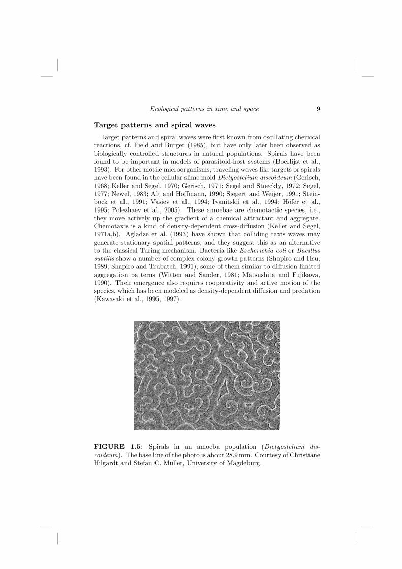
Target patterns and spiral waves were first known from oscillating chemicalreactions, cf. Field and Burger (1985), but have only later been observed asbiologically controlled structures in natural populations. Spirals have beenfound to be important in models of parasitoid-host systems (Boerlijst et al.,1993). For other motile microorganisms, traveling waves like targets or spiralshave been found in the cellular slime mold Dictyostelium discoideum (Gerisch,1968; Keller and Segel, 1970; Gerisch, 1971; Segel and Stoeckly, 1972; Segel,1977; Newel, 1983; Alt and Hoffmann, 1990; Siegert and Weijer, 1991; Stein-bock et al., 1991; Vasiev et al., 1994; Ivanitskii et al., 1994; Hofer et al.,1995; Polezhaev et al., 2005). These amoebae are chemotactic species, i.e.,they move actively up the gradient of a chemical attractant and aggregate.Chemotaxis is a kind of density-dependent cross-diffusion (Keller and Segel,1971a,b). Agladze et al. (1993) have shown that colliding taxis waves maygenerate stationary spatial patterns, and they suggest this as an alternativeto the classical Turing mechanism. Bacteria like Escherichia coli or Bacillussubtilis show a number of complex colony growth patterns (Shapiro and Hsu,1989; Shapiro and Trubatch, 1991), some of them similar to diffusion-limitedaggregation patterns (Witten and Sander, 1981; Matsushita and Fujikawa,1990). Their emergence also requires cooperativity and active motion of thespecies, which has been modeled as density-dependent diffusion and predation(Kawasaki et al., 1995, 1997).
FIGURE 1.5: Spirals in an amoeba population (Dictyostelium dis-coideum). The base line of the photo is about 28.9 mm. Courtesy of ChristianeHilgardt and Stefan C. Muller, University of Magdeburg.

10 Spatiotemporal patterns in ecology and epidemiology
New routes to spatiotemporal chaos
Space also provides new routes to chaotic dynamics. The emergence ofdiffusion-induced spatiotemporal chaos along a linear nutrient gradient hasbeen found by Pascual (1993) in a Rosenzweig-MacArthur phytoplankton-zooplankton model. Chaotic oscillations behind propagating diffusive frontsare found in a prey–predator model (Sherratt et al., 1995, 1997). Furthermore,it has been shown that the appearance of chaotic spatiotemporal oscillations ina prey–predator system is a somewhat more general phenomenon and need notbe attributed to front propagation or to an inhomogeneity of environmentalparameters (Petrovskii and Malchow, 1999; Petrovskii and Malchow, 2001b;Petrovskii et al., 2003; Petrovskii and Malchow, 2001a; Petrovskii et al., 2005).
Patterns of biological invasion and epidemic spread
A problem of increasing concern is the spread of non-native species andepidemic diseases (Drake and Mooney, 1989; Pimentel, 2002; Sax et al., 2005;Allen and Lee, 2006). Biological invasions are regarded as one of the mostsevere ecological problems, being responsible for the extinction of indigenousspecies, sustainable disturbance of ecosystems, and economic damage. There-fore, there is an increasing need to control and manage invasions. This re-quires an understanding of the mechanisms underlying the invasion process.Recently, many factors have been identified that affect the speed and the pat-tern of the spatial spread of an introduced species or pathogen, such as spatialheterogeneity, resource availability, stochasticity, environmental borders, pre-dation, competition, infection, etc.; cf. recent reviews by Fagan et al. (2002),Hastings et al. (2005), Hilker et al. (2005), Holt et al. (2005), and Petrovskiiet al. (2005). Mathematics, mathematical modeling, and computer scienceplay an increasing if not central role in exploring, understanding and predict-ing these complex processes. This is especially true in studies of biologicalinvasions where laboratory experiments cannot embrace appropriate spatialscales, and manipulative field experiments are, if at all ethically acceptable,very expensive, potentially dangerous, and lack the necessary time series.
The transmission dynamics of infectious diseases is one of the oldest top-ics of mathematical biology. As early as 1760, Daniel Bernoulli provided thefirst known mathematical result of epidemiology, that is, the defense of thepractice of inoculation against smallpox (Brauer and Castillo-Chavez, 2001).The amount of works in this area has exploded in the last decades. Differentaspects are dealt in the literature, from human health assessment to environ-mental assessment.
Chapter 2
An overview of modeling approaches
The great variety of different environmental settings and ecological interac-tions existing in mother nature requires, in order to make their theoreticalstudy more effective, an equally broad range of modeling approaches. Quitetypically, an adequate model choice depends not only on the ecosystem orcommunity type, but also on the goals of the study, in particular, on thespatial and/or temporal scales where the given phenomena are developing.Discreteness of populations is a fundamental property (cf. Durrett and Levin,1994), yet on a spatial scale much larger than the size of a typical individ-ual description of the population dynamics by a continuous quantity such asthe population density (the number of individuals of a given species per unitarea or unit volume) was proved to be effective, e.g., see Murray (1989) andShigesada and Kawasaki (1997). On a larger scale, however, environmentalheterogeneity and habitat fragmentation become important, which may makespace-discrete models more appropriate. A similar duality arises in the tem-poral dynamics. Moreover, due to the possible overlapping of spatial and/ortemporal scales associated with different processes, sometimes a hybrid ap-proach might be required that describes some of the processes continuouslyand some of them discretely; one example is given by a fish school feeding onplankton (Medvinsky et al., 2002).
The very first step to be done in choosing the model is a decision about the“state variables,” i.e., the quantities that give sufficient (for the purposes ofa given study) information about the state of the system. There is an appar-ent fundamental difference between the modeling approaches that take intoaccount each individual separately, cf. “individual-based modeling,” and theapproaches that describe the system state in a collective way, e.g., by means ofintroducing the population density. Obviously, an individual-based approach1
gives more information about the population system than an approach basedon the population density; however, its disadvantage is that this informationcan rarely be obtained other than through extensive numerical simulations.On the contrary, the density-based models often allow rigorous mathemati-cal analysis and analytical treatment. Another important distinction is thatpredictions of individual-based approaches are usually restricted to the spa-
1For the basics and state-of-the-art in that field, an interested reader is advised to checkthe books by DeAngelis and Gross (1992) and Grimm and Railsback (2005).
11

12 Spatiotemporal patterns in ecology and epidemiology
tial scales compatible with either size or motion of a single individual whiledensity-based approaches are valid on a larger scale.
Having chosen a density-based approach, the next step is to decide whetherdetails of system’s spatial structure may be important. In case they are not,then one arrives at a nonspatial model where the population density or densi-ties are functions of time but not of space. Specific mathematical settings forwriting down the model depend on whether the dynamics of a given popula-tion is more adequately described as time-discrete or time-continuous. Theformer approach works better for the populations with nonoverlapping gen-erations, the latter is valid when the generations are tangled. Throughoutthis book, we will mostly focus on the second case; a relevant mathematicaltechnique is then given by ordinary differential equations:
dUi(t)dT
= fi(U1, U2, . . . , Un) , i = 1, . . . , n , (2.1)
where Ui is the population density of the ith species at time T , n is the numberof species in the community, and functions fi take into account effects of birthand mortality; in most biologically meaningful situations, the functions fi arenonlinear with respect to at least some of their arguments.
Now, a very subtle issue is the decision about how many equations shouldthe system (2.1) contain and (a closely related question) what are the prop-erties of functions fi, which define the species responses and the types ofinterspecific interactions. Obviously, the population community even in avery simple ecosystem consists of dozens (more typically, hundreds or eventhousands) of different species. Therefore, an idea to write a separate equa-tion for each species is totally unrealistic. One way around this difficultyis to consider some “functional groups” instead of particular species. Moststraightforwardly, these groups would correspond to different trophic levels.A classical example is given by phytoplankton and zooplankton; although inany natural aquatic ecosystem each of these two groups consists of many dif-ferent species (sometimes interacting with each other in a very complicatedway), ecologists use these rough “binary” description quite successfully, inboth empirical and theoretical studies. Correspondingly, application of themodel (2.1) to the plankton system dynamics would result in a two-speciesprey–predator system.
An alternative approach to minimize the number of equations in (2.1) is tofocus on the dynamics of particular species. The reasons behind the choiceof those “key species” depends on the ecosystem properties but also on thepurpose of the study; for instance, in the case of biological invasion, oneof them should obviously be the alien pest. The system (2.1) then may bereduced to either just a single equation or to a few-species system described bytwo or three equations, e.g., accounting for the given species and its immediateconsumers or competitors. The impact of other species can be taken intoaccount in an indirect way by means of either adjusting parameter values(e.g., introducing additional mortality rates in order to account for other

An overview of modeling approaches 13
predators) or by including additional terms into the equations, cf. “closureterms” (van den Bosch et al., 1988; Steele and Henderson, 1992a; Edwardsand Yool, 2000).
Note that, while the predictive power of the few-species “conceptual” mod-els is usually not very high, they are very important in a wider theoreticalaspect because they make it possible to study the implications of basic inter-specific interactions thoroughly.
It should be also mentioned that, apart from the population dynamics, thegeneric system (2.1) has been effectively used for modeling the dynamics ofinfectious diseases, up to a somewhat different meaning of the state variables(such as density of susceptibles instead of density of prey, etc.) and to thechoice and meaning of the functions fi, e.g., see Busenberg and Cooke (1981),Capasso (1993), and Dieckmann et al. (2002).
Once the model is specified, the next step is to reveal its main propertiessuch as existence and stability of the steady states, existence of periodic so-lutions, solution boundedness, invariant manifold(s), etc. Careful analyticalstudy of these issues often requires application of some rather advanced math-ematical techniques; cf. Part II. The goal of this analysis is twofold. First,the model must be biologically reasonable and thus should exclude some ob-viously artificial situations (such as, for instance, population growth from avanishingly small value of the population density). Second – and this is, infact, the principal idea of a mathematical modeling approach – a change in themodel properties with respect to a change in a certain controlling parameteris usually assumed to reflect the changes in the dynamics of the given natural(eco)system and thus has immediate biological implications.
The system (2.1) creates an appropriate modeling framework in the caseof a “well-mixed” community in a homogeneous environment, i.e., when thecommunity may be in all circumstances regarded as spatially homogeneous.Obviously, this is not always the case, and this affects the model choice. Forinstance, the spatial structure of a given population or community can bepredefined by the environmental heterogeneity. In the case of small environ-mental gradients, a relevant mathematical model can still be space-continuous;however, in an extreme case of large environmental gradients or a fragmentedhabitat, a space-discrete approach will sometimes be more insightful. A math-ematical model would then consist of a few systems such as (2.1) where dif-ferent systems describe the dynamics of different subpopulations,2 being cou-pled together due to migration between the habitats (Jansen and Lloyd, 2000;Jansen, 2001; Petrovskii and Li, 2001).
A separate branch of space-discrete models is made by metapopulation mod-els (Gilpin and Hanski, 1991; Hanski, 1999), where the state of the “metacom-
2In the time-discrete case, a model would consist of coupled difference equations or maps;cf. Comins et al. (1992); Allen et al. (1993).

14 Spatiotemporal patterns in ecology and epidemiology
munity” may be described by variables other than population density, e.g.,giving a proportion of all sites where the given species is present.
Another source of spatial heterogeneity is the formation of self-organizedpatterns as a result of inter- and intra-specific interactions, and this is goingto be the main focus of this book.
Obviously, for the spatial aspect of population dynamics to be nontrivial,there must exist a mechanism of population redistribution in space. The mostcommon one is due to individual motion. The motion can be either active(i.e., due to self-motion) or passive (e.g., when an individual of an air-bornespecies is carried about by wind). Also, motion can take place with or withouta preferred direction. The simplest (but yet biologically meaningful) case isgiven by random isotropic motion, i.e., diffusion. In Chapter 8, we will talk inmore details about diffusion in the population dynamics; for the moment wesimply assume that the spatial aspects can be taken into account by addingthe diffusion terms to Equations (2.1):
∂Ui(R, T )∂T
= Di∇2Ui(R, T ) + fi(U1, U2, . . . , Un) (2.2)
(i = 1, . . . , n), where R = (X,Y, Z) is the position in space, Di is the diffusioncoefficient of the ith species, and ∇2 is the Laplace operator:
∇2 =∂2
∂X2+
∂2
∂Y 2+
∂2
∂Z2.
The system (2.2) is a system of nonlinear partial differential equations and,as such, is a difficult mathematical object to study. Although some regularanalytical approaches are available [e.g., see Petrovskii and Li (2006) andalso Chapter 9 of this book], more often its properties are studied throughcomputer simulations by means of solving Equations (2.2) numerically (cf.Thomas, 1995).
Correspondingly, the next important step is scaling. In analytical ap-proaches it may be easier to work with the original systems (2.1) or (2.2)because it sometimes makes the interpretation of the results more straight-forward. In numerical simulations, however, we actually work with numbersrather than with dimensional quantities. Therefore, it is more convenient tofirst transform a given model to a dimensionless form. Remarkably, it is al-ways possible; the corresponding procedure is usually called either dimensionsanalysis or scaling. Indeed, the functions fi depend not only on the populationdensities but also on a number of parameters, such as the birth/death rate(s),population carrying capacity(-ies), etc. These parameters provide an intrinsicscale for each of the variables. Some typical examples showing how to do it inpractice are given below; a very general description of the procedure3 along
3It should be mentioned here that scaling by itself is a powerful method of analysis, and itoften allows one to arrive at some important conclusions without even specifying the model;see Barenblatt (1996).
An overview of modeling approaches 15
with its application to a wide range of problems can be found in Barenblatt(1996).
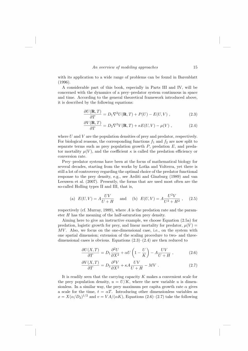
A considerable part of this book, especially in Parts III and IV, will beconcerned with the dynamics of a prey–predator system continuous in spaceand time. According to the general theoretical framework introduced above,it is described by the following equations:
∂U(R, T )∂T
= D1∇2U(R, T ) + P (U)− E(U, V ) , (2.3)
∂V (R, T )∂T
= D2∇2V (R, T ) + κE(U, V )− µ(V ) , (2.4)
where U and V are the population densities of prey and predator, respectively.For biological reasons, the corresponding functions f1 and f2 are now split toseparate terms such as prey population growth P , predation E, and preda-tor mortality µ(V ), and the coefficient κ is called the predation efficiency orconversion rate.
Prey–predator systems have been at the focus of mathematical biology forseveral decades, starting from the works by Lotka and Volterra, yet there isstill a lot of controversy regarding the optimal choice of the predator functionalresponse to the prey density, e.g., see Arditi and Ginzburg (1989) and vanLeeuwen et al. (2007). Presently, the forms that are used most often are theso-called Holling types II and III, that is,
(a) E(U, V ) = AUV
U + Hand (b) E(U, V ) = A
U2V
U2 + H2, (2.5)
respectively (cf. Murray, 1989), where A is the predation rate and the param-eter H has the meaning of the half-saturation prey density.
Aiming here to give an instructive example, we choose Equation (2.5a) forpredation, logistic growth for prey, and linear mortality for predator, µ(V ) =MV . Also, we focus on the one-dimensional case, i.e., on the system withone spatial dimension; extension of the scaling procedure to two- and three-dimensional cases is obvious. Equations (2.3)–(2.4) are then reduced to
∂U(X,T )∂T
= D1∂2U
∂X2+ αU
(1− U
K
)−A
UV
U + H, (2.6)
∂V (X,T )∂T
= D2∂2V
∂X2+ κA
UV
U + H−MV . (2.7)
It is readily seen that the carrying capacity K makes a convenient scale forthe prey population density, u = U/K, where the new variable u is dimen-sionless. In a similar way, the prey maximum per capita growth rate α givesa scale for the time, t = αT . Introducing other dimensionless variables asx = X(α/D2)1/2 and v = V A/(αK), Equations (2.6)–(2.7) take the following

16 Spatiotemporal patterns in ecology and epidemiology
forms:
∂u(x, t)∂t
= ε∂2u
∂x2+ u(1− u)− uv
u + h, (2.8)
∂v(x, t)∂t
=∂2v
∂x2+ k
uv
u + h−mv , (2.9)
where k = κA/α, m = M/α, h = H/K, and ε = D1/D2 are dimensionlessparameters. Correspondingly, the properties of u(x, t) and v(x, t) now dependnot on all the original parameters separately but only on their combinationsk, m, h, and ε.
Note that (2.8)–(2.9) contain fewer parameters than the original Equations(2.6)–(2.7), i.e., four instead of eight. A decrease in parameter number due tothe transition to dimensionless variables is a typical result. It gives anotheradvantage of scaling: The less parameters a given model contains, the moreeffective is its study by means of numerical simulations.
An important remark that should be made here is that in most cases thechoice of dimensionless variables is not unique. Indeed, talking about theprey–predator system (2.6)–(2.7), it is readily seen that we can introducedimensionless variables as t = T (κAK/H), x = X(κAK/(D2H))1/2, u =U/K, and v = V/(κK). From Equations (2.6)–(2.7), we then obtain:
∂u(x, t)∂t
= ε∂2u
∂x2+ au(1− u)− uv
1 + αu, (2.10)
∂v(x, t)∂t
=∂2v
∂x2+
uv
1 + αu−mv , (2.11)
where α = K/H, a = ηHK/(κA), m = MH/(κAK), and ε = D1/D2.Unfortunately, there are no accepted standards regarding the scaling proce-
dure, and which of these two schemes to choose4 is to a large extent a matterof personal preference. Different authors use different schemes, and that of-ten makes quantitative comparisons between published results rather difficult,even in the case when the principal implications are clear.
Prey–predator interactions are ecologically meaningful but surely they donot exhaust all possible types of interspecific interactions. Another impor-tant case is given by competition. In contrast to the prey–predator system,where predation is beneficial for one species and detrimental for the other,competition hampers the population growth of both involved species. Math-ematically, it is usually described by a bilinear function, i.e., a general time-and space-continuous model of a community of N competing species looks as
4There can be some variations within each of these two approaches, such as using D1 insteadof D2 for scaling X, or X can be scaled to the domain length, etc.
An overview of modeling approaches 17
follows:
∂Ui(R, T )∂T
= Di∇2Ui(R, T ) +
(αi −
∑rijUj
)Ui , (2.12)
i = 1, . . . , N
(cf. May, 1973), where αi is the inherent population growth rate of the ithspecies and R = (rij) is the so-called “community matrix.” In a general case,rij 6= rji because different species possess different abilities for competition.
The properties of the competing species system appear to be significantlydifferent from those of a prey–predator system. In particular, it is readilyseen that, contrary to a prey–predator system where cycles are generic, anonspatial system of two competing species cannot have periodic solutionsbut only equilibrium states.
In agreement with the general idea of scaling, the number of parameters in(2.12) can be reduced (by means of choosing relevant scaling factors for thepopulation densities, space, and time) from N2 + 2N to N2 + N − 2. Oneparticular case will be considered in Section 10.3.
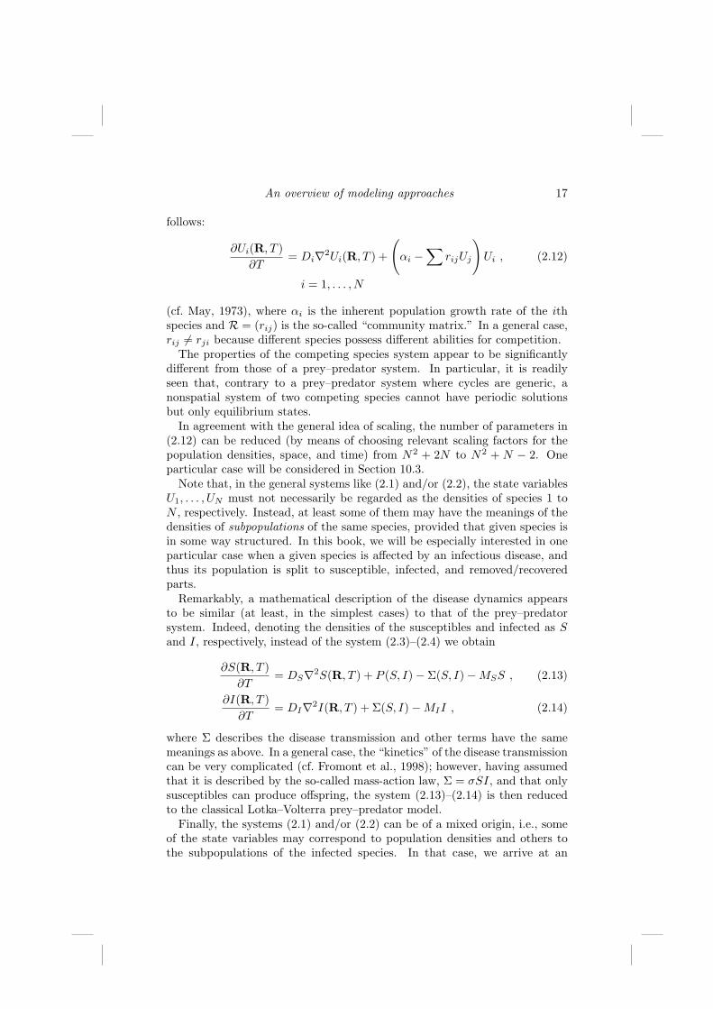
Note that, in the general systems like (2.1) and/or (2.2), the state variablesU1, . . . , UN must not necessarily be regarded as the densities of species 1 toN , respectively. Instead, at least some of them may have the meanings of thedensities of subpopulations of the same species, provided that given species isin some way structured. In this book, we will be especially interested in oneparticular case when a given species is affected by an infectious disease, andthus its population is split to susceptible, infected, and removed/recoveredparts.
Remarkably, a mathematical description of the disease dynamics appearsto be similar (at least, in the simplest cases) to that of the prey–predatorsystem. Indeed, denoting the densities of the susceptibles and infected as Sand I, respectively, instead of the system (2.3)–(2.4) we obtain
∂S(R, T )∂T
= DS∇2S(R, T ) + P (S, I)− Σ(S, I)−MSS , (2.13)
∂I(R, T )∂T
= DI∇2I(R, T ) + Σ(S, I)−MII , (2.14)
where Σ describes the disease transmission and other terms have the samemeanings as above. In a general case, the “kinetics” of the disease transmissioncan be very complicated (cf. Fromont et al., 1998); however, having assumedthat it is described by the so-called mass-action law, Σ = σSI, and that onlysusceptibles can produce offspring, the system (2.13)–(2.14) is then reducedto the classical Lotka–Volterra prey–predator model.
Finally, the systems (2.1) and/or (2.2) can be of a mixed origin, i.e., someof the state variables may correspond to population densities and others tothe subpopulations of the infected species. In that case, we arrive at an

18 Spatiotemporal patterns in ecology and epidemiology
ecoepidemiological system. We will provide a detailed consideration of thecorresponding models in Chapter 7.
All the models mentioned above are deterministic in the sense that they aredescribed by deterministic equations. As such, they largely neglect the impactof stochastisity and noise. To distinguish between the cases when stochastisitymay or may not be important is a highly nontrivial problem. Indeed, althoughthe population dynamics is intrinsically stochastic, in many cases it is very welldescribed by the deterministic equations. In practice, the choice of the model(i.e., deterministic or stochastic) is often purely heuristic. Also, it of coursedepends on the goals of the study. In order to take into account possibleeffects of stochastisity and noise, one can either apply statistical modeling(cf. Czaran, 1998) or include stochastic terms/factors into the deterministicmodel. The latter approach will be used in Part IV of this book, where wemake an insight into the issue and reveal, by means of considering severalspecific cases, how the system’s dynamics can be modified by the impact ofstochastisity.

Part II
Models of temporaldynamics
19


Chapter 3
Classical one population models
Population theory, with its long history, dates back to the Malthus model,formulated for economic reasons in the early nineteenth century, predicting thepopulation problems due to an exponential growth not supported by unlimitedresources. The basic equation was then corrected by Verhulst (1845; 1847) tocompensate for the shortcomings of the earlier model. The logistic equationstates instead the existence of a horizontal asymptote to which the populationtends as time flows. This asymptote has a biological interpretation, namelythe carrying capacity the environment possesses, to support the populationdescribed by the model.
Later on, in the twenties of the past century, the works by Lotka andVolterra extended the mathematical modeling to prey–predator situations(Lotka, 1925; Volterra, 1926a,b). Since then the field has developed, andthe biomathematical literature is now very large.
In this chapter we present the basic models in population theory, at firstconsidering an isolated population and in Section 3.2 models including mi-grations. The purpose of Section 3.1 is to introduce some basic notation andterminology, while in Section 3.2 the most elementary bifurcations will natu-rally arise from the analysis. We stress the fact that in some cases the effort ismade to keep the considerations simple enough to help the less familiar readerto grasp the basic concepts. Also, occasionally very elementary examples aremade in both this as well as in subsequent chapters. In Section 3.3, simplediscrete versions of the basic one-population models are discussed, to pave theway for the topic of the following Section 3.4, a short introduction of chaos.
3.1 Isolated populations models
Consider a single population in an idealized situation, in which neitherdeaths nor migration occur. Since then the only process that can happen isreproduction, the population must be a function of time T , i.e., U ≡ U(T ).Taking the time unit to be months, for instance, suppose we count the indi-viduals at different times and find the following results:
U(0) = 1000, U(10) = 1200, U(20) = 1440.
21
22 Spatiotemporal patterns in ecology and epidemiology
If we take the population differences first with respect to the origin and thenwith respect to the previous measurement, we find
U(10)− U(0) = 200, U(20)− U(0) = 440, U(40)− U(20) = 240.
One question we may ask is, how do we know the estimate size of the pop-ulation at intermediate times, such as U(1) and U(2)? An intuitive answerwould then be U(1) = 1020, U(2) = 1044. The reason is that we tend tothink linearly in terms of time. If 200 newborns occur in a time of 10 months,we expect 20 in just one. In other words, we are saying that the monthlyincrement in population is δU = 20.
Suppose now we take a second population, V (T ), in the same environmentalconditions, the situation from the previous case differing only in the initialconditions. We would then find
V (0) = 2000, V (10) = 2400, V (20) = 2880,
again as 1000 individuals contribute 200 newborns in 10 months. The reasonis once again that we also think linearly in terms of the population size.However, in this case we have
V (10)− V (0) = 400, V (20)− V (0) = 880, V (40)− V (20) = 480.
Thus, comparing the examples, the monthly population increment δV = 40 6=δU must be a function of population size V , δV ≡ δV (V ).
Consider a third example, again in different environmental circumstances,but still not accounting for deaths and migrations, in which the population Fis counted at other times giving the following data:
F (T0) = 100, F (T1) = 105, F (T2) = 110.
We may now ask which of the two populations F or U reproduces faster. Now,taking differences, we find
F (T1)− F (T0) = 5, F (T2)− F (T1) = 5, F (T2)− F (T0) = 10,
and these absolute numbers seem to be smaller than the previous ones, so thatwe may think that F reproduces the slowest. But if time is now measuredin weeks, so that T1 = 1, T2 = 2, and we make the proportions, clearly Freproduces the fastest of all populations. Indeed, at the end of one month,keeping the same growth proportion, we find F (1) = 120, and at the end of10 months then F (10) = 300, assuming here that newborns do not start toreproduce in the whole period taken into account. The absolute increment isthe same as for U , but here the percentage increase is clearly different. Indeed,in 10 months the increase of F was 200%, while the one of U was only 20%.This indicates first of all that the population increment is also a function oftime,
δF ≡ ∆F ≡ F (T + ∆T )− F (T ) ≡ δF (T ).

Classical one population models 23
Secondly, we should take the reference value of the population into account,thus not speaking of absolute increases, but rather of percentage accruals, i.e.,relative increases ∆F/F .
The simplest form for the population population increment over time thatwe can write is then
1U
∆U
∆T≡ 1
UR(U) ≡ rM (U) = r,
with rM = r denoting a constant. Dimensionally, U is a number, and R(U) isthen a per capita rate, i.e., a per capita frequency of reproduction. The word“per capita” refers to the fact that we were naturally induced to divide bythe whole population size U , to determine the individual reproduction rate.The function rM (U) is then the individual frequency of reproduction, in thiscase constant. Equivalently, the function R(U) is thus a linear function ofU, R(U) = rU . Finally, we can let the time interval tend to zero, to get adifferential equation. We have thus obtained the Malthus model,
dU
dT(T ) = rU(T ), (3.1)
in which case the (constant) function rM = r denotes the per capita instaneousreproduction rate. More generally, as seen before, it may be a function of time.The equation is dimensionally sound as on the left there is a rate measured innumbers by time, and on the right a frequency times a number. Its solutionis easily obtained:
U(T ) = U(0) exp(rT ), (3.2)
with U(0) denoting the initial value of the population. The problem with thismodel is that for r > 0, the solution goes to ∞, while for r < 0, it goes tozero.
To correct this behavior Verhulst proposed the following modification. Theconstant r should be replaced by a function, namely, the simplest nonconstantfunction of the population, rL(U), which implicitly becomes a function oftime. This means that it should be taken as a linear function of U , namely,rL ≡ rL(U) = r(1 − U
K ). Notice indeed that the slope of this straight linemust be negative, since otherwise rL would be bounded below by the earlierconstant r, and therefore the solution of the corrected equation would alsobe bounded below by the exponential function of the Malthus equation; thus,for a positive slope, the modification will not solve the problem, because thesolution would still diverge for large times. We thus have the logistic equation
dU
dT(T ) = r
(1− U(T )
K
)U(T ), (3.3)
in which now geometrically r has the meaning of the intercept at the originand therefore must be nonnegative; otherwise, as seen above, the population
24 Spatiotemporal patterns in ecology and epidemiology
will vanish. The solution of (3.3) can be analytically evaluated, by separationof variables,
dU
(1− UK )U(T )
=dU
U(T )+
dU
K(1− UK )
= [d ln(U)− d ln(1− U
K)] = d ln(
U
1− UK
) = rdT,
followed by integration, to give
lnU
1− UK
= rT + C,U
1− UK
= exp(C) exp(rT ) ≡ C0 exp(rT )
and finally
U(t) =C0K exp(rT )
K + C0 exp(rT ). (3.4)
Thus, for T → ∞, the solution tends to a horizontal asymptote, U → K.The value of this constant represents the population that the environmentcan support in the long run, and it is called the carrying capacity. It alsorepresents the root of the linear function r(U) in the RU phase plane. Noticethat R(U) ≥ 0 for 0 ≤ U ≤ K, and conversely for U ≥ K. It thus followsthat in the logistic equation, dU
dT ≥ 0 for 0 ≤ U ≤ K, and dUdT ≤ 0 for
U ≥ K, thus implying that U must grow when it has a value below K, whileit should decrease when it exceeds it. These qualitative results then confirmthe analysis we performed above: In both cases the population ultimatelytends to the value K. Notice finally that, as mentioned earlier, for r < 0the solution obtained also shows that U → 0 as T → ∞, allowing us to thendiscard this case for the reproduction parameter.
A further second order correction consists in taking a parabola instead of astraight line for the reproduction function, namely,
rA ≡ rA(U) = r(U −B)(1− U
K), 0 < B < K,
where again we take r > 0 in view of the previous discussion, so that thedifferential equation now takes into account the impact of the Allee effect:
dU
dT(T ) = r(U −B)(1− U
K)U(T ). (3.5)
In this model the reproduction function rA becomes negative for populationvalues smaller than B. This models the well-known fact that for small popu-lations that live in a large environment in which individuals cannot easily findeach other, reproduction becomes difficult. The phase plane analysis showsthat the equilibria now are the same as for the logistic model, the origin, andthe carrying capacity K, but there is also the equilibrium at the value B.
Classical one population models 25
The rate of change of the population is positive only for B < U < K, so thatagain K is a stable equilibrium since U tends to grow if it is B < U < K anddecreases to this value if it exceeds it. For the equilibrium B, the reverse istrue, thus, as just seen, U increases away from it if it is larger than B, butif 0 ≤ U < B, then the derivative is negative so that in such case U → 0+,meaning that ultimately the population vanishes, but from positive values.Thus, in the above-described environment, the population will be wiped awaywhen it drops below a threshold population value represented by B. A furtherdifference with the logistic model is given by the fact that here K is not aglobally asymptotically equilibrium, while in the logistic case it is. Startingfrom any value of U , indeed, in the latter case K is ultimately reached, whilefor the Allee model (3.5), this is not true for 0 ≤ U ≤ B.
3.1.1 Scaling
Let us consider now the effect of scaling. Taking into account the Malthusmodel, with a net growth rate r ∈ R that may be positive or negative, let usrescale the variables by setting
U(T ) = βu(t), T = αt. (3.6)
The constants β and α must be positive, because biologically we account onlyfor nonnegative populations and since we look at the future evolution of thesystem. By suitably differentiating we find
dU(T )dT
=β
α
du(t)dt
, (3.7)
and substituting into Malthus equation upon simplification we have
du(t)dt
= αru(t). (3.8)
In view of α > 0 and r ∈ R, we cannot impose rα = 1, but rather considerthe two cases rα = ±1, i.e., work separately with the two equations
du(t)dt
= u(t),du(t)
dt= −u(t).
This is not practical, so in the case of unrestricted net growth rate for theMalthus model, adimensionalization does not bring too much of an advantage.In the case of the logistic model, instead we must have r > 0, otherwise themodel would show the population to have a negative carrying capacity to keepthe “crowding competition” term negative, i.e., to still ensure − r
K U2 < 0. Inany case, the growth of the population would always be negative, leading toits disappearance, and thus vanifying the benefit of the introduction of thecorrection term. In the logistic case with r > 0, scaling can be performed

26 Spatiotemporal patterns in ecology and epidemiology
0 5 10 15−1
−0.5
0
0.5
1
r M
U
per capita reproduction functions r(U)
0 5 10 15−20
−10
0
10
20
RM
U
reproduction functions R(U)
0 5 10 15−0.5
0
0.5
1
U
r l
0 5 10 15−2
−1
0
1
2
U
r A
0 5 10 15−2
−1
0
1
2
3
U
Rl
0 5 10−10
−5
0
5
10
U
RA
0 1 20
5
10
15
20
UM
t
Malthus, logistic and Allee solutions U(t)
0 2 4 60
5
10
t
Ul
0 2 4 60
5
10
t
UA
FIGURE 3.1: The rows refer to the three models considered: the first rowto the Malthus model (3.1), the second one to the logistic one (3.3), and thethird one to the Allee model (3.5). The first column contains the picture ofthe per capita reproduction function r(U), the second one the reproductionfunction R(U), and the last one the analytic solution of each model for threedifferent initial conditions and for each value of the function r(U) plottedin the corresponding row. In the logistic and Allee models, however, we donot show the case r < 0 as it is not meaningful. For the Malthus growth,a negative net growth function leads to the disappearance of the population.For the logistic model, all solutions tend to the horizontal asymptote; forthe Allee model, this is the case only if the initial conditions are above thethreshold value B, corresponding to the extra root, with respect to the logisticcase, of the reproduction function in the second column.
with the same substitutions indicated above to get
du(t)dt
= αru(t)(
1− βu(t)K
)= u(1− u), (3.9)

Classical one population models 27
with the choice β = K and α = r−1. For the Allee model (3.5), again assumingr > 0 and using the same substitutions, we find
du(t)dt
= αru(t)(βu(t)−B)(
1− βu(t)K
)= u(u− b)(1− u), (3.10)
choosing β = K, α = (Kr)−1 and setting b = BK−1 < 1.
3.2 Migration models
Consider now a population U(T ) that does not reproduce; rather, it issubject only to a constant rate migration m and competition for resources.Its evolution equation then reads
dU
dT= m− U2 ≡ f(U). (3.11)
From the logistic model we take the quadratic death rate term, while theconstant term represents the external feed (or loss) of new individuals. Indeed,if we take m < 0, the first term represents an emigration term, and seekingequilibria, there is no way of zeroing out the right-hand side, as U2 = −mhas no real roots. Thus the population U will decrease at all times as in theUf phase plane, f(U) = 0 is a parabola always below the horizontal axis.For m = 0, i.e., no migration of any sort occurs, the same parabola will moveupwards and become tangent to the U axis at the origin. The origin will thenbecome a semistable equilibrium, but the behavior of the model will essentiallybe unchanged. A more interesting situation arises for an immigration ratem > 0. In such a case there are two real roots, U± = ±√m. The parabolaf(U) is above the U axis in between them, so that f(U) ≥ 0 for U− ≤ U ≤ U+,and therefore U grows in such an interval and decreases for U ≥ U+. Thismeans that the equilibrium U+ is stable, and conversely U− < 0 is unstable,but since it is unfeasible, we disregard it. When m increases, so does U+.By drawing a picture of U+ as a function of U we obtain what is called abifurcation diagram; see Figure 3.2.
We can also consider a more complex situation, a logistic model in whichwe allow the growth rate r to be of either sign. In such a case, the modelshould not be written as (3.3) of Section 3.1 because the term containing thecarrying capacity would become positive for r < 0, which does not correspondto the population pressure. We then write instead
dU
dT= aU − bU2, (3.12)

28 Spatiotemporal patterns in ecology and epidemiology
0 2 4 6 8 10 12 14 16 18 20−5
−4
−3
−2
−1
0
1
2
3
4
5
mu
U−
U+
FIGURE 3.2: Bifurcation diagram for the logistic model (3.11), with im-migration and no reproduction, dU/dT = m−U2 ≡ f(U). The stable feasiblebranch is represented by ∗; we also show the infeasible unstable branch .
with a ∈ R and b ≥ 0. Let us rescale the equations by introducing newpositive parameters α and β, so that U = βu and T = αt give
dU
dT= β
du
dt
dt
dT=
β
α
du
dt
and the rescaled model becomes
du
dt= aαu− bαβu2. (3.13)
Now we can choose the free parameters so as to simplify the equation, but thechoice aα = 1 is not possible, because in such a case the growth rate a wouldbe positive. If we want to account for a ∈ R, we then need to take bαβ = 1,i.e., β = 1
bα , and therefore we must then set aα = abβ ≡ µ ∈ R. The rescaled
model then readsdu
dt= µu− u2 ≡ F (u). (3.14)
The equilibria are the origin and the point um = µ ∈ R. The parabola F (u)is positive once again in between the roots, implying with the discussion asabove that the right root is always stable and the left one is unstable. Forµ < 0, the right root is the origin, while for µ > 0 it is the point um > 0.At µ = 0, the origin is a double root, a semistable equilibrium in this case,as it seems stable if approached from the right and unstable from the left.If we draw the roots as function of the parameter µ, we find the diagram of
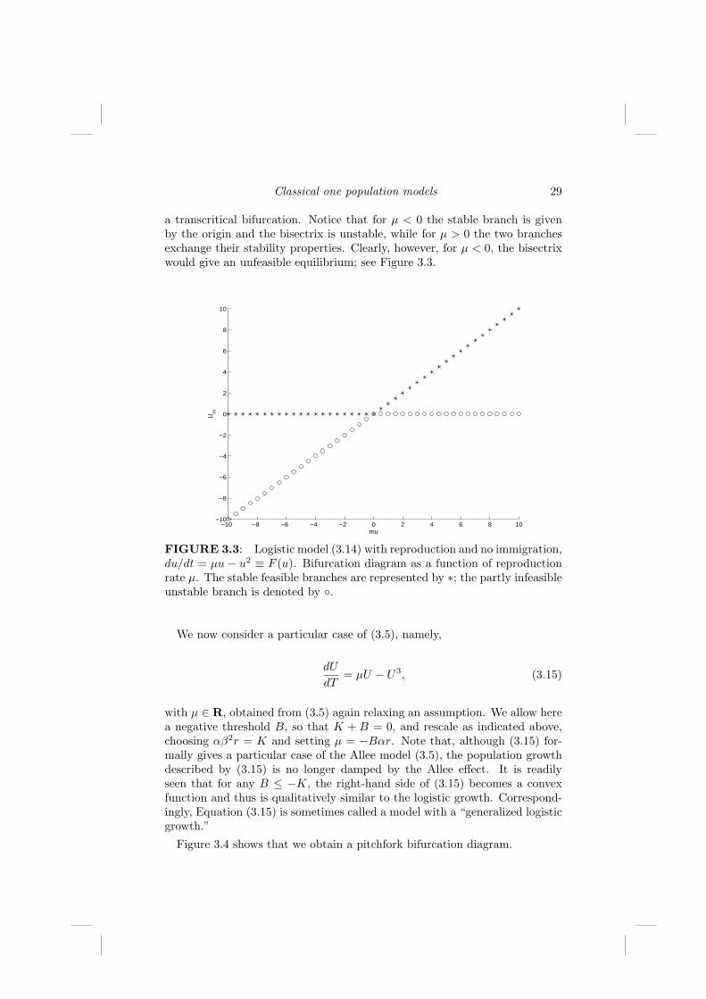
Classical one population models 29
a transcritical bifurcation. Notice that for µ < 0 the stable branch is givenby the origin and the bisectrix is unstable, while for µ > 0 the two branchesexchange their stability properties. Clearly, however, for µ < 0, the bisectrixwould give an unfeasible equilibrium; see Figure 3.3.
−10 −8 −6 −4 −2 0 2 4 6 8 10−10
−8
−6
−4
−2
0
2
4
6
8
10
mu
Um
FIGURE 3.3: Logistic model (3.14) with reproduction and no immigration,du/dt = µu − u2 ≡ F (u). Bifurcation diagram as a function of reproductionrate µ. The stable feasible branches are represented by ∗; the partly infeasibleunstable branch is denoted by .
We now consider a particular case of (3.5), namely,
dU
dT= µU − U3, (3.15)
with µ ∈ R, obtained from (3.5) again relaxing an assumption. We allow herea negative threshold B, so that K + B = 0, and rescale as indicated above,choosing αβ2r = K and setting µ = −Bαr. Note that, although (3.15) for-mally gives a particular case of the Allee model (3.5), the population growthdescribed by (3.15) is no longer damped by the Allee effect. It is readilyseen that for any B ≤ −K, the right-hand side of (3.15) becomes a convexfunction and thus is qualitatively similar to the logistic growth. Correspond-ingly, Equation (3.15) is sometimes called a model with a “generalized logisticgrowth.”
Figure 3.4 shows that we obtain a pitchfork bifurcation diagram.

30 Spatiotemporal patterns in ecology and epidemiology
−3 −2 −1 0 1 2 3 4−2
−1.5
−1
−0.5
0
0.5
1
1.5
2
mu
Um
FIGURE 3.4: Bifurcation diagram for a generalized logistic growth (3.15),dU/dT = µU−U3. The pitchfork bifurcation occurs at the origin. The stablebranches are represented by ∗; there is one that is infeasible. The unstablebranch is denoted by .
3.2.1 Harvesting
We now consider a term H(U) denoting harvesting of the population,
dU(T )dT
= R(U)−H(U).
The exploitation term can generally be chosen in one of the following ways:
H(U) = h, H(U) = hU, H(U) = hU
A + U,
or H(U) = hU2
A + U2, (3.16)
where A and h are positive parameters. The first two expressions in (3.16) cor-respond to constant and linear exploitation, respectively, allowing for possiblyunbounded harvests if the population is large enough. The last two assume anupper bound on the return, in a sense analogous to the limitations providedby the logistic equation. They differ essentially near the origin, the formerstarting with a slope at the origin, while the last one has zero derivative there.Compare Figures 3.11 and 3.13.
Combining now different types of harvestings of the population, let us lookin detail at its consequences, with respect to the different growth mechanisms
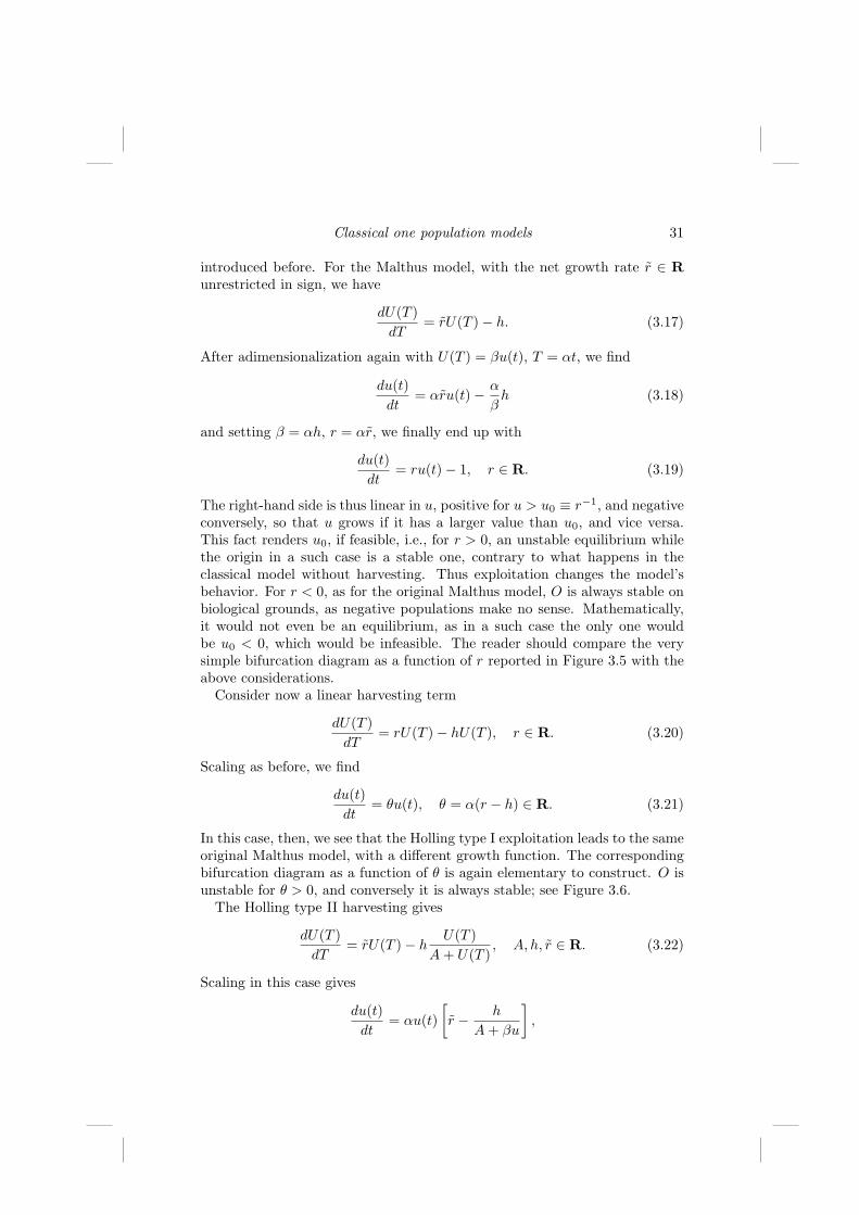
Classical one population models 31
introduced before. For the Malthus model, with the net growth rate r ∈ Runrestricted in sign, we have
dU(T )dT
= rU(T )− h. (3.17)
After adimensionalization again with U(T ) = βu(t), T = αt, we find
du(t)dt
= αru(t)− α
βh (3.18)
and setting β = αh, r = αr, we finally end up with
du(t)dt
= ru(t)− 1, r ∈ R. (3.19)
The right-hand side is thus linear in u, positive for u > u0 ≡ r−1, and negativeconversely, so that u grows if it has a larger value than u0, and vice versa.This fact renders u0, if feasible, i.e., for r > 0, an unstable equilibrium whilethe origin in a such case is a stable one, contrary to what happens in theclassical model without harvesting. Thus exploitation changes the model’sbehavior. For r < 0, as for the original Malthus model, O is always stable onbiological grounds, as negative populations make no sense. Mathematically,it would not even be an equilibrium, as in a such case the only one wouldbe u0 < 0, which would be infeasible. The reader should compare the verysimple bifurcation diagram as a function of r reported in Figure 3.5 with theabove considerations.
Consider now a linear harvesting term
dU(T )dT
= rU(T )− hU(T ), r ∈ R. (3.20)
Scaling as before, we find
du(t)dt
= θu(t), θ = α(r − h) ∈ R. (3.21)
In this case, then, we see that the Holling type I exploitation leads to the sameoriginal Malthus model, with a different growth function. The correspondingbifurcation diagram as a function of θ is again elementary to construct. O isunstable for θ > 0, and conversely it is always stable; see Figure 3.6.
The Holling type II harvesting gives
dU(T )dT
= rU(T )− hU(T )
A + U(T ), A, h, r ∈ R. (3.22)
Scaling in this case gives
du(t)dt
= αu(t)[r − h
A + βu
],
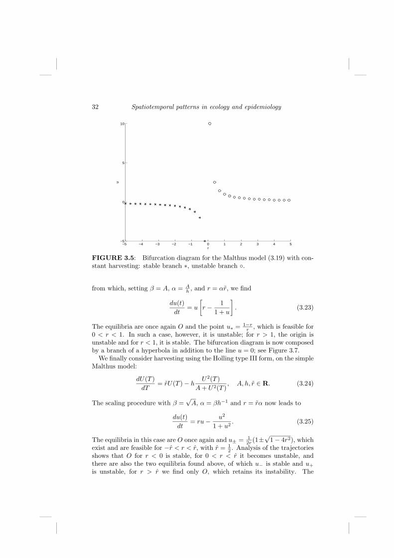
32 Spatiotemporal patterns in ecology and epidemiology
−5 −4 −3 −2 −1 0 1 2 3 4 5−5
0
5
10
r
u
FIGURE 3.5: Bifurcation diagram for the Malthus model (3.19) with con-stant harvesting: stable branch ∗, unstable branch .
from which, setting β = A, α = Ah , and r = αr, we find
du(t)dt
= u
[r − 1
1 + u
]. (3.23)
The equilibria are once again O and the point u∗ = 1−rr , which is feasible for
0 < r < 1. In such a case, however, it is unstable; for r > 1, the origin isunstable and for r < 1, it is stable. The bifurcation diagram is now composedby a branch of a hyperbola in addition to the line u = 0; see Figure 3.7.
We finally consider harvesting using the Holling type III form, on the simpleMalthus model:
dU(T )dT
= rU(T )− hU2(T )
A + U2(T ), A, h, r ∈ R. (3.24)
The scaling procedure with β =√
A, α = βh−1 and r = rα now leads to
du(t)dt
= ru− u2
1 + u2. (3.25)
The equilibria in this case are O once again and u± = 12r (1±√1− 4r2), which
exist and are feasible for −r < r < r, with r = 12 . Analysis of the trajectories
shows that O for r < 0 is stable, for 0 < r < r it becomes unstable, andthere are also the two equilibria found above, of which u− is stable and u+
is unstable, for r > r we find only O, which retains its instability. The

Classical one population models 33
−4 −3 −2 −1 0 1 2 3 4−1
−0.8
−0.6
−0.4
−0.2
0
0.2
0.4
0.6
0.8
1
r
u
FIGURE 3.6: Bifurcation diagram for the Malthus model (3.21) withHolling type I harvesting: stable branch ∗, unstable branch .
bifurcation diagram (see Figure 3.8) exhibits once again an unstable branchof a hyperbola in the interval 0 < r < r, which coalesces with the stablebranch emanating from O at the point u = 1. The latter is easily calculatedby imposing tangence between the straight line and the Holling type III term,yielding the equations
ru =u2
1 + u2, r =
2u
(1 + u2)2.
Substitution of one into the other easily leads to 1 + u2 = 2, from which thevalues of u and r are obtained, in agreement with what was formerly obtained.
We now will consider the logistic model subject to the various forms ofexploitation. As mentioned before, here we will assume r > 0, which willgive an alternative choice for the rescaling. In particular, we will constructbifurcation diagrams now as functions of the harvesting effort h. We have,under constant effort,
dU(T )dT
= rU(T )(
1− U(T )K
)− h, h > 0. (3.26)
Rescaling with the usual substitutions and setting β = K, α = r−1, andh = hr−1 gives the adimensional model
du(t)dt
= u(1− u)− h. (3.27)

34 Spatiotemporal patterns in ecology and epidemiology
−2 −1.5 −1 −0.5 0 0.5 1 1.5 20
5
10
15
20
25
r
U*
FIGURE 3.7: Bifurcation diagram for Malthus model with Holling type IIharvesting (3.23): stable branch ∗, unstable branch .
Clearly the right-hand side represents the logistic parabola through the originand the normalized carrying capacity K = 1 pulled down by an amount h.Its roots are intersections of this parabola with the horizontal straight line atheight h. They then move toward each other the higher h becomes, retainingtheir stability properties, stable on the right and unstable on the left, untilthey coalesce and then disappear, at which point the origin becomes the onlystable equilibrium of the system. The coalescence point concides with thevertex of the parabola, thus it occurs for h = 1
4 . The bifurcation diagram(Figure 3.9) thus shows a parabola with a stable and an unstable branch, whilethe origin for h > 0 is always stable. Biologically, this constant harvestingeffort thus has on the equilibria the same effect of the Allee model withoutexploitation. Notice also that in fisheries models the level of the harvestingeffort at the stable equilibrium gives the so-called maximum sustainable yieldof the exploitation.
We now turn to Holling type I harvest namely,
dU(T )dT
= rU(T )(
1− U(T )K
)− hU(T ), h > 0. (3.28)
Scaling givesdu(t)
dt= u(1− h− u), (3.29)
with the choices αr = 1, β = K and setting h = hα. In this case, the stableequilibrim at u = 1 for h = 0 moves leftwards linearly with h, as it is given

Classical one population models 35
−2 −1.5 −1 −0.5 0 0.5 1 1.5 20
5
10
15
20
25
r
U−
U
+
FIGURE 3.8: Bifurcation diagram for Malthus model with Holling typeIII harvesting (3.25): stable branch ∗, unstable branch .
by us = 1 − h, retaining its stability, until it hits the origin at h = 1. Thiscorresponds to the logistic and harvesting curves to be tangent to each otherat O. The origin that was formerly unstable at this point becomes stable andremains so for every h ≥ 1. Figure 3.10 shows the corresponding bifurcationdiagram.
The Holling type II exploitation gives
dU(T )dT
= rU(T )(
1− U(T )K
)− h
U(T )A + U(T )
, A, h > 0. (3.30)
Upon rescaling we find for α = r−1, β = A, θ = AK ,
du(t)dt
= u(1− θu)− hu
1 + u≡ P (u)− H(u). (3.31)
Notice that the slopes of the parabola P and the hyperbola H can be evaluatedso that at the origin they are, respectively,
dP
du= 1− 2θu,
dH
du=
h
1 + u2,
dP
du
∣∣∣∣u=0
= 1,dH
du
∣∣∣∣∣u=0
= h.
The equilibria are given by
u± =12θ
[1− θ ±
√(θ + 1)2 − 4hθ
].

36 Spatiotemporal patterns in ecology and epidemiology
0 0.1 0.2 0.3 0.4 0.5 0.6 0.7 0.8 0.9 10
0.1
0.2
0.3
0.4
0.5
0.6
0.7
0.8
0.9
1
h
u
FIGURE 3.9: Bifurcation diagram for the logistic model (3.27) with con-stant harvesting: stable branch ∗, unstable branch .
They are real only for h < hs ≡ (θ+1)2
4θ . In such a case, the rightmost one,u+, is stable, as the hyperbola given by the harvesting term lies above thelogistic parabola for u > u+, and conversely for u < u−. The leftmost one,u−, will instead be unstable. Feasibility is better described geometrically. Weneed to ensure that the curves P (u) and H(u) meet in the first quadrant.For low values of h, this is always ensured, 0 < h < 1, but for h > 1, thishappens only if the value of the horizontal asymptote of H is below the vertexof the parabola P , of height (4θ)−1. Thus, for 1 < h < (4θ)−1, there are theintersections u± described above, and for this to occur, naturally we needto require θ < 1
4 . In the contrary case, no intersection between P and H ispossible for h > 1, and the origin becomes the only equilibrium of the system.Figure 3.11 shows these situations. Notice also that the origin is always astable equilibrium when u± are feasible, and is instead ustable for 1 > h > 0.The bifurcation diagram is reported in Figure 3.12.
The logistic growth subject to Holling type III exploitation is ruled by theequation
dU(T )dT
= rU(T )(
1− U(T )K
)− h
U2(T )A + U2(T )
, A, h > 0. (3.32)
The rescaling is now done with α = r−1, β =√
A, and setting h = hr√
A,
φ =√
AK , to get
du(t)dt
= u(1− φu)− hu2
1 + u2≡ u[(u)− H(u)]. (3.33)

Classical one population models 37
0 0.2 0.4 0.6 0.8 1 1.2 1.4 1.6 1.8 20
0.1
0.2
0.3
0.4
0.5
0.6
0.7
0.8
0.9
1
h
u
FIGURE 3.10: Bifurcation diagram for the logistic model (3.29) with lin-ear harvesting: stable branch ∗, unstable branch .
This shows that O is again an equilibrium while the other ones come fromsolving (u) = H(u). The analysis of H(u) shows that it has a maximumlocated at (1, 1
2h) and an inflection point at Q ≡ (√
3,√
34 h). We can then
choose (u) through Q and with a height at the origin located between theheights of the two former points, so that then 1
2h > 1 >√
34 h. These give
the interval 2 < h < 4√3. The condition ensuring that (u) goes through Q is
easily found to be φ = 1√3− h
4 , and the constraint φ > 0 is satisfied since it
is equivalent to the former requirement 1 >√
34 h. Thus, in these conditions
there are three intersections, otherwise just one. The two different situationsare shown in Figure 3.13. The origin is always an unstable equilibrium ofthe system. If there is only one other equilibrium, it is then stable (Figure3.14). If there are three more, the intermediate of the two is unstable, whilethe other two are stable (see Figure 3.15).
Notice also that Figure 3.15 shows the phenomenon of hysteresis. Namely,starting from the population being exploited at the carrying capacity in ab-sence of harvesting, h = 0, the equilibrium is the uppermost on the verticalaxis. Increasing the exploitation, the stable upper branch of the bifurcationis followed, with the equilibrium decreasing steadily and slowly for increasingh. However, when h ≈ .85 ≡ hc, the upper critical level, the two stable andunstable branches coalesce, the upper equilibrium for larger harvesting effortsthen disappears, and sudddenly the population moves toward the only stableequilibrium, which is now situated very near the horizontal axis. If we think

38 Spatiotemporal patterns in ecology and epidemiology
0 10 20 30 400
2
4
6
8
10
12
u
P, H
0 0.1 0.2 0.30
0.05
0.1
0.15
0.2
0.25
0.3
u
P, H
FIGURE 3.11: Diagram of the right hand-side for the logistic model (3.31)with Holling type II exploitation, on the left for K = 33.3, i.e., φ = 0.3, andfor integer harvesting rates h ∈ 1, . . . , 10. On the right is a blowup of thesame picture around the origin for h ∈ 0.5, 1, 1.5, 2, 2.5
now to go back to the previous situation only by diminishing the harvestingto values just below the critical one, say at h = 0.8, the reached stable equilib-rium on the lower branch of the bifurcation diagram moves upwards, but onlyby a very small amount. This is, of course, provided that the whole ecosys-tem has not collapsed before due to some external disturbances that push thepopulation u to zero. Thus we have the counter-intuitive fact that it is notenough to backtrack a little to push the system to its previous situation. Itis not until h = 0.2 ≡ hc, the lower critical value, that u recovers, as in sucha case following toward the left the lower branch of the bifurcation diagram,the lower stable equilibrium vanishes and the system is pushed suddenly up-wards to the stable branch near the carrying capacity. On increasing againthe harvesting effort h, the cycle would then be repeated.
We finally turn to the analysis of the Allee model, coupled with harvesting:
dU(T )dT
= rU(T )(U(T )−B)(
1− U(T )K
)− h, h > 0. (3.34)
The adimensionalization procedure in this case, letting β = K, α = (Kr)−1,and h = hK−2r−1, b = B
K , gives the rescaled model
du(t)dt
= u(u− b)(1− u)− h. (3.35)

Classical one population models 39
0 0.2 0.4 0.6 0.8 1 1.2 1.4 1.6 1.8 20
0.1
0.2
0.3
0.4
0.5
0.6
0.7
0.8
0.9
1
h
u
FIGURE 3.12: Bifurcation diagram for the logistic model (3.31) withHolling type II harvesting: stable branch ∗, unstable branch .
The equilibria are found geometrically to move from the values b and 1 towardeach other, until they coalesce and disappear, as the cubic in the right-handside is “pulled down” by an amount h. Mathematically, O is not a root of theright-hand side, but biologically it remains a stable equilibrium of the system.The other two retain their type of stability, namely, the one emanating fromb is unstable and the one coming from 1 remains stable. Figure 3.16 showsthe bifurcation diagram.
For linear exploitation, the unscaled model reads
dU(T )dT
= rU(T )(U(T )−B)(
1− U(T )K
)− hU(T ), h > 0. (3.36)
Adimensionalization is carried out almost as above, with β = K, α = (Kr)−1,and h = h(Kr)−1, b = B
K , to get
du(t)dt
= u[(u− b)(1− u)− h]. (3.37)
This shows that O is always an equilibrium and stable since linearization(i.e., dropping the higher order terms, which vanish faster near 0) gives du
dt ≈−(b+h)u. Then there are two other, coming from “pulling down” the parabolawith roots in b and 1, so that these roots, as above, approach each other andretain their stability properties. The corresponding bifurcation diagram isgiven in Figure 3.17.

40 Spatiotemporal patterns in ecology and epidemiology
0 10 20 30 400
1
2
3
4
5
6
7
8
9
u
P, H
0 0.1 0.2 0.30
0.05
0.1
0.15
0.2
0.25
0.3
u
P, H
FIGURE 3.13: Diagram of right-hand side for Holling type III exploitation(3.33), on the left for K = 33.3, i.e., φ = 0.3, and for integer harvesting ratesh ∈ 1, . . . , 10. On the right is a blowup of the same picture around theorigin for h ∈ 0.5, 1, 1.5, 2, 2.5. The lowmost harvesting curve intersersectsthe reproduction curve at two feasible points, and the other ones at four suchpoints.
For a Holling type II harvesting, the unscaled Allee model is
dU(T )dT
= rU(T )(U(T )−B)(
1− U(T )K
)− h
U(T )A + U(T )
, A, h > 0. (3.38)
Rescaling is performed choosing β = A, α = (Ar)−1, and h = hA−2r−1,b = B
A , φ = AK , to find
du(t)dt
= u(u− b)(1− φu)− hu
1 + u. (3.39)
The equilibria in addition to the origin, stable, are two points moving towardeach other for increasing h from b and φ−1, the former unstable and the latterstable. Then they coalesce and disappear, leaving only the origin as stableequilibrium. Figure 3.18 shows the bifurcation diagram.
The Allee model with Holling type III harvesting is
dU(T )dT
= rU(T )(U(T )−B)(
1− U(T )K
)− h
U2(T )A + U2(T )
(3.40)
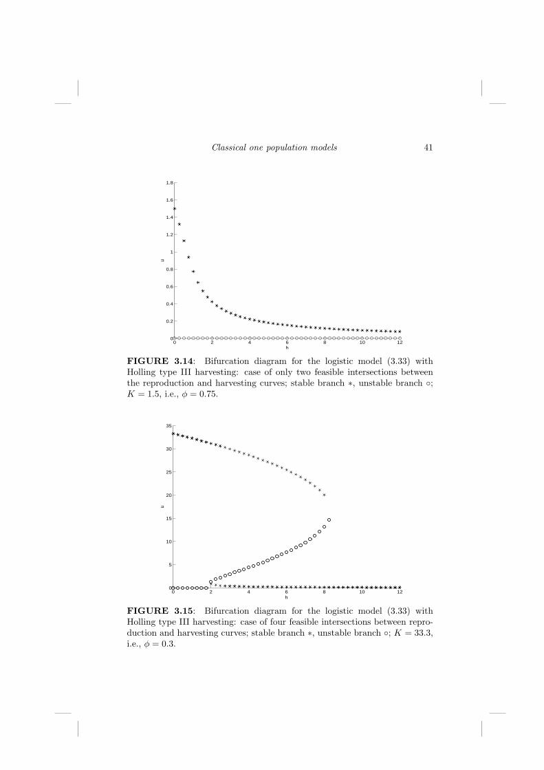
Classical one population models 41
0 2 4 6 8 10 120
0.2
0.4
0.6
0.8
1
1.2
1.4
1.6
1.8
h
u
FIGURE 3.14: Bifurcation diagram for the logistic model (3.33) withHolling type III harvesting: case of only two feasible intersections betweenthe reproduction and harvesting curves; stable branch ∗, unstable branch ;K = 1.5, i.e., φ = 0.75.
0 2 4 6 8 10 120
5
10
15
20
25
30
35
h
u
FIGURE 3.15: Bifurcation diagram for the logistic model (3.33) withHolling type III harvesting: case of four feasible intersections between repro-duction and harvesting curves; stable branch ∗, unstable branch ; K = 33.3,i.e., φ = 0.3.
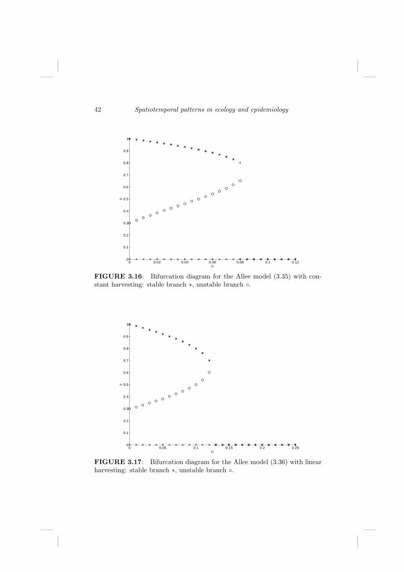
42 Spatiotemporal patterns in ecology and epidemiology
0 0.02 0.04 0.06 0.08 0.1 0.120
0.1
0.2
0.3
0.4
0.5
0.6
0.7
0.8
0.9
1
h
u
FIGURE 3.16: Bifurcation diagram for the Allee model (3.35) with con-stant harvesting: stable branch ∗, unstable branch .
0 0.05 0.1 0.15 0.2 0.250
0.1
0.2
0.3
0.4
0.5
0.6
0.7
0.8
0.9
1
h
u
FIGURE 3.17: Bifurcation diagram for the Allee model (3.36) with linearharvesting: stable branch ∗, unstable branch .

Classical one population models 43
0 0.05 0.1 0.15 0.2 0.250
0.1
0.2
0.3
0.4
0.5
0.6
0.7
0.8
0.9
1
h
u
FIGURE 3.18: Bifurcation diagram for the Allee model (3.39) with Hollingtype II harvesting: stable branch ∗, unstable branch .
(with A, h > 0), and rescaling via β =√
A, α = (√
Ar)−1, and h = αh(√
A)−1,b = B√
A, φ =
√A
K , leads to
du(t)dt
= u(u− b)(1− φu)− hu2
1 + u2. (3.41)
The equilibria are again the origin and the two points moving toward eachother from b and φ−1, retaining their stability, until they coalesce and vanish.The bifurcation diagram is shown in Figure 3.19.
On comparing Figures 3.16–3.19, we notice that they are only quantita-tively different, but their qualitative behavior is exactly the same. This agreeswith previous remarks on the intersections of the reproduction and harvestingfunctions.
There is a further remark we ought to make. On comparing Figures 3.16 to3.19 with Figure 3.15, where we have seen the hysteresis phenomenon occur,again qualitatively we see that the behavior for the Allee model is similar, butfor one important feature. Namely, this model entails the sure disappearanceof the population once the critical harvesting effort hC is reached. In thiscase, indeed, the lower branch of the bifurcation diagram lies exactly on thehorizontal axis so that the population vanishes and thus cannot recover evenby drastically reducing the exploitation down to h = 0. The only difference,as remarked above for the four cases of harvesting in the Allee situation, isthe increasing value of hC , namely, hC = 0.08 for constant effort, hC = 0.12for Holling type I effort, hC = 0.2 for Holling type II effort, and hC = 0.28for Holling type III effort.

44 Spatiotemporal patterns in ecology and epidemiology
0 0.1 0.2 0.3 0.4 0.50
0.1
0.2
0.3
0.4
0.5
0.6
0.7
0.8
0.9
1
h
u
FIGURE 3.19: Bifurcation diagram for the Allee model with Holling typeIII harvesting (3.41): stable branch ∗, unstable branch .
3.3 Glance at discrete models
We finally consider here models in which the population size is measured atfixed time intervals, in general corresponding to generation times. Let Tn bethe instants in time corresponding to the appearance of the new generation;it could be eggs disclosure for some insects, for instance, which may happen afew times during a good season. Therefore, the new generation of size Xn ≡X(Tn) may appear a number of times a year, depending on the species underconsideration and the climactic factors. The quantity Xn+1 − Xn measuresthe change in the population size during one such typical generation, and inabsence of migrations, it is the balance of births and deaths, namely, Xn+1 −Xn = bXn−dXn = rXn, where b and d denote the per capita birth and deathrates per generation time. What we have described is a version of the discreteMalthus model,
Xn+1 = aXn, a = 1 + r = 1 + b− d. (3.42)
Attempting the solution of this difference equation by means of a discreteexponential function Xn = αn, we obtain the characteristic equation α =a, from which the solution Xn = X0α
n follows. This model exhibits thesame drawbacks as its continuous counterpart, namely, for a < 1 we findXn → 0+, and for a > 1 we have Xn → +∞. But a new problem arisesfor −1 < a < 0, since now the solution oscillates taking negative values,

Classical one population models 45
which is clearly a nonbiological situation. A natural correction would requireXn+1 = maxaXn, 0.
An improvement would be to consider logistic-type models, of which thefollowing are examples:
Xn+1 =aXn
Xn + A, (3.43)
Xn+1 =aX2
n
X2n + A
, (3.44)
Xn+1 = Xn + aXn
(1− Xn
K
), (3.45)
Xn+1 = a
(1− Xn
K
), (3.46)
Xn+1 = ea(1−XnK ), (3.47)
Xn+1 = aXn
(1− Xn
K
)−β
. (3.48)
In general, these models are of the form Xn+1 = f(Xn), and if X∗ existssuch that X∗ = f(X∗), so that it is a fixed point for the map f , then itis an equilibrium of the discrete system. We now consider a perturbation,un = Xn−X∗, so that for a suitable X ∈ CHX∗, Xn, with the symbol CHdenoting the convex hull of the points X∗, Xn, i.e., the smallest interval thatcontains them, Taylor’s formula gives
Xn+1 −X∗ = f(Xn)− f(X∗) (3.49)
=df
dX(X∗)un +
12
d2f
dX2(X)u2
n ≡ ρun +12
d2f
dX2(X)u2
n.
Since upon linearization we have un+1 = ρun = ρ2un−1 = . . . = ρn+1u0,convergence occurs if
|ρ| < 1. (3.50)
Finally, let us mention a very famous model, due to Fibonacci, that givesrise to a “second order” difference equation, namely, it involves the two pre-vious generations to determine the next one, xn+1 = xn + xn−1, with initialconditions x0 = 0, x1 = 1. Its solution involves the golden ratio, which isrelated to the length of the side of the regular decagon, the polygon with 10sides. Indeed, upon trying an exponential solution, we find the characteristicequation
α2 − α− 1 = 0, (3.51)
whose solutions are α± = 12 [1±√5]. Now the solution of the Fibonacci model
can be written as a linear combination of exponentials with these bases:
xn = c+αn+ + c−αn
− = c+12[1 +
√5]n + c−1
2[1−
√5]n

46 Spatiotemporal patterns in ecology and epidemiology
so that as n →∞, since |α−| < 1, we have
xn+1
xn→ 1
2[1 +
√5] = α+ ≡ φ = 1.61803399.
In classical euclidean geometry, the golden ratio φ is determined by the pointα that splits the (unit) segment in two parts, so as to satisfy the proportion1 : α = α : (1−α) = φ. On expanding, φ = α
1−α = 1α and φ is the only positive
solution of the resulting quadratic equation, i.e., (3.51), so that φ = α+.
3.4 Peek into chaos
Let us specifically investigate Equation (3.45). We find
f(X) = (1 + a)X − a
KX2,
df
dX= 1 + a− 2a
KXn.
Calculating the fixed points of f , we find the equilibria of the equation, X∗ = 0and X∗ = K. To study the stability, we are led to the characteristic equationand the consequent conditions ρ = df
dX (X∗) = dfdX (0) = |1 + a| < 1, which
implies the stability condition 0 > a > −2, so that for a > 0, the originis unstable, and ρ = df
dX (X∗) = dfdX (K) = |1 − a| < 1, which gives instead
0 < a < 2 for stability. Now, to see what happens for a > 2, we can considerthe iterated map Xn+2 = f2(Xn),
f2(X) = f(f(X)) = (1 + a)f(X)− a
Kf(X)2
= (1 + a)2X −X2(a + 1)a(a + 2)
K+
2a2
K2(1 + a)X3 − a3
K3X4.
To find the equilibria f2(X) = X, we must then solve the following quarticequation:
aX(1− X
K)[( a
K
)2
X2 − a(a + 2)X
K+ a + 2
]= 0,
which has the roots X = 0, X = K, and
X± =K2
2a2
a
K(a + 2)±
[a2
K2(a + 2)2 − 4
K2(a + 2)a2
] 12
=K
2a
[(a + 2)±
√a2 − 4
]. (3.52)

Classical one population models 47
The latter are real for a ≥ 2. Moreover, observe that
f(X+) = X+ + aX+
(1− X+
K
)= (1 + a)X+ − a
KX2
+
= (1 + a)a + 22a
K +1 + a
2aK
√a2 − 4
− a
K
K2
4a2
[(a + 2)2 + a2 − 4 + 2(a + 2)
√a2 − 4
]
=√
a2 − 4[1 + a
2aK − K
2a(a + 2)
]+
K
2a
[(1 + a)(2 + a)− (a2 + 2a)
]
=K
2a
[(2 + a)(a + 1− a)−
√a2 − 4
]=
K
2a
[2 + a−
√a2 − 4
]= X−.
Since we have a fixed point for the iterated map, it follows that
X+ = f2(X+) = f(f(X+)) = f(X−), i.e. X−f(X+), X+ = f(X−).
We have thus found a periodic solution for f(X), of period 2, for a > 2. We in-vestigate now the stability of this periodic solution. Recalling the convergencecondition (3.50) for fixed point iterates of the map f2(X), let us differentiatef2(X)−X = 0. Since X+ solves the quadratic equation (3.52), we find
df2
dX(X+)− 1 = a
(X+ −
X2+
K
)[2
a2
K2X+ − a
K(a + 2)
]
=K
2
(a + 2 +
√a2 − 4
) 12a
(a− 2−
√a2 − 4
)·
· a
K
[(a + 2 +
√a2 − 4
)− a− 2
]
=14
[a2 −
(2 +
√a2 − 4
)2]√
a2 − 4
=14
[a2 − 4− 4
√a2 − 4− (a2 − 4)
]√a2 − 4 = 4− a2.
Hence df2dX (X+) = 5−a2 and the condition for stability then becomes |5−a2| <
1, so that the cycle of period 2 for the map f is stable for the parameter range2 < a <
√6.
The question now arises as to what happens for a >√
6. Again a periodicsolution of period 4 can be found that is stable for
√6 < a < 2.544. Iterating
the question and the procedure, a periodic solution of period 8 arises hereafter,which is stable for 2.544 < a < 2.564. On continuing this procedure, we obtainthe so-called period doubling route to chaos. It can be shown that if an is theparameter value for which a periodic solution of period 2n appears, then
limn→∞
an+1 − an
an+2 − an+1= 4.6692016... ,
this limiting value being known as the Feigenbaum constant.


Chapter 4
Interacting populations
The Lotka–Volterra model takes its name from the authors of the first in-vestigations of interacting populations. Volterra (1926a; 1926b; 1931) basedhis considerations on the unexpected results of the field observations of thebiologist D’Ancona (1954) on the fishing catches in the Adriatic sea after theFirst World War. Other models were developed later to avoid the main draw-back of the original Lotka–Volterra model, namely, the neutral stability of itsinterior equilibrium point. This makes the solutions sensitive to variationsof the initial conditions of the system, and therefore biologically they are notvery satisfactory. These modifications include at first quadratic models, whichincorporate a logistic growth term for at least one of the two populations, andthen also other nonlinear terms, such as the effect of satiation in feeding.
Competing situations and species living in symbiosis are other examplesof interacting populations, extended then to more complicated food webs inwhich the species at a certain level in the chain is the predator of those in thelevels below and a prey for the higher level ones.
To model the quadratic interactions between different populations, we pro-ceed similarly to what is done for the logistic term in a single populationgrowth. If one individual of the first population U wanders in the environ-ment, the meetings with individuals of the second population V will occur ata certain per capita rate α. Thus the total encounters of that specific individ-ual per unit time are αV . But this must be multiplied by every individual ofspecies V , so that the total number of interactions in the time unit betweenthe two populations is then αUV . More generally, the interactions for thepopulation V are described by a per capita rate f(U, V )V . The quadraticcase then corresponds to a Holling type I term. If we want to model thesaturation effect experienced by predators when the prey abound, we shouldthen take for f a Holling type II or III function. The latter correspond towhat in operations research is called the law of diminishing returns, for thesame amount of effort the gain is larger if the effort is small, and tends to aplateau for increasing efforts.
In this chapter we consider basically the Lotka–Volterra model and its mod-ifications. In addition to presenting the models, we also develop the mainmathematical techniques needed for the analysis of these systems, by dis-cussing very simple situations in detail. We start with an example in Section4.1 that mathematically illustrates the local stability analysis and the tools
49

50 Spatiotemporal patterns in ecology and epidemiology
needed for it. In Section 4.2 a more in-depth discussion of the Lotka–Volterramodel is related and also used for a more in-depth discussion of the scalingprocedure, also in view of the later parts of the book. Section 4.2.1 presentsanother modification of the prey–predator system and the other interesting bi-ological situations of competing and symbiotic species. Quadratic and otherclassical nonlinear models are discussed. The main mathematical tool forstudying the global stability of these models is the Lyapunov function, pre-sented in Section 4.3.1. Then the question of the investigation of possible limitcycles is addressed, with Section 4.3.2 giving positive and negative criteria.
The last two sections are devoted to a step further, beyond the two-speciesmodels. In Section 4.3.3, a four-level food web is considered, from mineralsthrough plants and herbivores up to the top predators, the carnivores. Section4.4 describes a very important problem in ecology, namely, the preservationof cultures, in this case vineyards, by using ecological controls.
From now on all parameters appearing in the models are assumed to benonnegative constants, unless otherwise specified.
4.1 Two-species prey–predator population model
We consider an idealized ecosystem in which only two populations are ac-counted for, and one may be hunted by the second one. More specifically,let the prey and the predator populations be denoted by U(T ) and V (T ),respectively. We assume that the environment provides enough resources forthe former to ensure its Malthusian growth. The predators instead show lo-gistic growth, where r denotes their reproduction rate and K represents theenvironment carrying capacity. These assumptions imply that the predatorshave sources of food other than the prey U . In the absence of interactions,the two populations would grow independently as follows:
dU
dT= αU(T ),
dV
dT= rV (T )
[1− V (T )
K
].
Assume now that the predation occurs at rate b, while the conversion rateinto new predators is described by the parameter c. Combining the aboveequations, we thus obtain
dU
dT= U(α− bV ),
dV
dT= rV
(1− V
K
)+ cUV. (4.1)
To analyze this system, we first find the nullclines, i.e., the lines in the phaseplane on which each population does not change. Their intersections also givethe equilibria of the system, i.e., the points at which both populations do notchange. The two nullclines are respectively defined by the equations dU
dT = 0,

Interacting populations 51
dVdT = 0, and these in turn give for the equilibria the system of algebraicequations
U(α− bV ) = 0, V
[r
(1− V
K
)+ cU
]= 0. (4.2)
Now, from the first one, we get either U(T ) ≡ U0 = 0 or V (T ) ≡ V2 = αb .
In the former case, from the second one, we have either V (T ) ≡ V0 = 0or V (T ) ≡ V1 = K. The second choice on the first equation gives, uponsubstitution into the second one, U(T ) ≡ U2 = r
c ( αbK − 1). Thus we have the
three equilibria
E0 ≡ (U0, V0) ≡ (0, 0), E1 ≡ (U0, V1) ≡ (0, V1), E2 ≡ (U2, V2).
Clearly E0 and E1 are always feasible, while to have a meaningful solution forE2 we need the populations to be nonnegative, and this entails the restrictionK < α
b , which is then the feasibility condition for E2.
Local Stability Analysis
We now study the long-term behavior of the model near the equilibria.To do so, we need to linearize it. The procedure consists in defining newvariables in the neighborhood of each equilibrium point and then disregardingperturbations of higher order, so that the system becomes easily integrable.Of course the solutions we find are valid only as a first approximation nearthe equilibrium, but nevertheless they tell a lot about the model’s behavior.
Consider E0 at first. We investigate what happens to the system in aneighborhood of the origin. As U, V in this case are small, namely U, V <1, then U2, V 2, UV < U, V so that U2, V 2, UV << 1. These second orderperturbations are much smaller than the original ones and can be disregardedas mentioned earlier. The system then simplifies to
dU
dT= αU(T ),
dV
dT= rV (T ). (4.3)
This is easy to solve, giving U(T ) = U(0) exp(αT ), V (T ) = V (0) exp(rT ). Infact, it is so easy because it is uncoupled. Since α, r > 0, the solutions willgrow, thus the trajectories will wander away from the origin, even though wechose U(0) = U0 ≈ 0, V (0) = V0 ≈ 0.
Look now at E1. In this case, U is still small, but V lies near the valueV1. It is therefore better to introduce the perturbation y = V − V1, for whichdydT ≡ dV
dT . Again we have y2, yU < y, so that y2, yU << 1 and the lattercan be disregarded. The first equation of the linearized system in a such casereads
dU
dT= U(T )[α− b(y + V1)] = U(T )[α− bV1] = U(T )[α− bK],

52 Spatiotemporal patterns in ecology and epidemiology
while the second one is
dy
dT= r(y + V1)
[1− (y + V1)
K
]+ cU(T )(y + V1)
= r(y + K)[1− (y + K)
K
]+ cU(T )(y + K)
= −r(y + K)y
K+ cKU(T ) = −ry + cKU(T ).
In this case the system is not so easy to solve. But substitution is still aviable method. Solve the first equation, which is still independent of y, to getU(T ) = U(0) exp[(α− bK)T ]. Substituting into the second equation, we find
dy
dT= − ry + cKU(0) exp[(α− bK)T ]. (4.4)
As no powers higher than one, nor product of unknown functions appear in it,this is a linear constant coefficient, first order nonhomogeneous ordinary dif-ferential equation. Notice that each expression has its own meaning, namely,the coefficients are indeed constants, not functions of time; the highest deriva-tive is the first one; there is a term independent of the unknown y making theequation nonhomogeneous, i.e., carrying it to the right-hand side; the latter isnonzero, i.e., nonhomogeneous; and, finally, no partial derivatives arise in theformulation. This classification may be useful for understandig how to solveit, if one wishes to look for the method in books. Instead, we will proceed ina constructive way. If we forget about the nonhomogeneous part, the solutionis easily found to be
y(T ) = k exp(−rT ), (4.5)
k denoting an arbitrary integration constant. This is just the solution of thehomogeneous equation. To find the one for our problem, we use the method ofvariation of parameters, which amounts to letting k become a function of time,k ≡ k(T ). Differentiation and substitution into the original nonhomogeneousequation give for the left-hand side
dy
dT=
d[k(T ) exp(−rT )]dT
=dk
dTexp(−rT ) + k(T )
d[exp(−rT )]dT
=dk
dTexp(−rT )− rk(T ) exp(−rT ),
while for the right-hand side we have
−ry(T ) + cKU(T ) = −rk(T ) exp(−rT ) + cKU(0) exp[(α− bK)T ].
Observe that two terms on the two sides of the equation are equal. Thus,equating and simplifying, we find
dk
dT= cK exp(rT )U(0) exp[(α− bK)T ] = cKU(0) exp[(α + r − bK)T ].
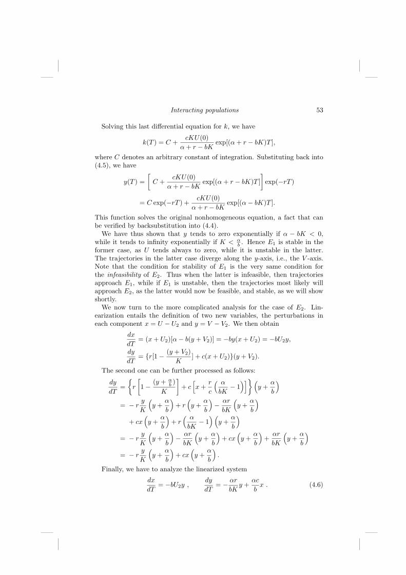
Interacting populations 53
Solving this last differential equation for k, we have
k(T ) = C +cKU(0)
α + r − bKexp[(α + r − bK)T ],
where C denotes an arbitrary constant of integration. Substituting back into(4.5), we have
y(T ) =[
C +cKU(0)
α + r − bKexp[(α + r − bK)T ]
]exp(−rT )
= C exp(−rT ) +cKU(0)
α + r − bKexp[(α− bK)T ].
This function solves the original nonhomogeneous equation, a fact that canbe verified by backsubstitution into (4.4).
We have thus shown that y tends to zero exponentially if α − bK < 0,while it tends to infinity exponentially if K < α
b . Hence E1 is stable in theformer case, as U tends always to zero, while it is unstable in the latter.The trajectories in the latter case diverge along the y-axis, i.e., the V -axis.Note that the condition for stability of E1 is the very same condition forthe infeasibility of E2. Thus when the latter is infeasible, then trajectoriesapproach E1, while if E1 is unstable, then the trajectories most likely willapproach E2, as the latter would now be feasible, and stable, as we will showshortly.
We now turn to the more complicated analysis for the case of E2. Lin-earization entails the definition of two new variables, the perturbations ineach component x = U − U2 and y = V − V2. We then obtain
dx
dT= (x + U2)[α− b(y + V2)] = −by(x + U2) = −bU2y,
dy
dT= r[1− (y + V2)
K] + c(x + U2)(y + V2).
The second one can be further processed as follows:
dy
dT=
r
[1− (y + α
b )K
]+ c
[x +
r
c
( α
bK− 1
)] (y +
α
b
)
= − ry
K
(y +
α
b
)+ r
(y +
α
b
)− αr
bK
(y +
α
b
)
+ cx(y +
α
b
)+ r
( α
bK− 1
)(y +
α
b
)
= − ry
K
(y +
α
b
)− αr
bK
(y +
α
b
)+ cx
(y +
α
b
)+
αr
bK
(y +
α
b
)
= − ry
K
(y +
α
b
)+ cx
(y +
α
b
).
Finally, we have to analyze the linearized system
dx
dT= −bU2y ,
dy
dT= − αr
bKy +
αc
bx . (4.6)

54 Spatiotemporal patterns in ecology and epidemiology
Let us introduce the perturbation vector u = (x, y)T . We can then writethe above system in the form du
dT = Mu, where the matrix M will now bedetermined. To do this in a very elementary but constructive way, let usobserve that for a generic matrix A with elements
A ≡[
A1,1 A1,2
A2,1 A2,2
],
upon postmultiplication by u ≡ (u1, u2)T , the row by column product givesthe vector
(A1,1u1 + A1,2u2, A2,1u1 + A2,2u2)T .
If we denote by A.,j the jth column of the matrix A, so that A ≡ [A.,1, A.,2],then the above equations can be rewritten as Au = A.,1u1 +A.,2u2. It is thenapparent that the jth column of the matrix A acts on the jth component ofu. To construct the matrix M , we have to look at its action on the vectoru, action coming from the equations of the system. From the first one, thecomponent u1 ≡ x is seen to be absent, while u2 ≡ y gets multiplied by −bU2.The only number that makes u1 disappear is zero. Similarly, in the secondequation, x is multiplied by αc
b . Hence the first column of M must be givenby [0, αc
b ]T . In the second equation, moreover, y has the coefficient − αrbK , so
that the second column of M must be given by [−bU2,− αrbK ]T . In summary,
A =[
0 − bU2αcb − αr
bK
].
If we consider carefully the matrix just obtained, we find that it coincides withthe Jacobian of the original system (4.1) evaluated at E2. This is a generalresult. Any time we linearize around an equilibrium, we may skip all the stepsundertaken above and just consider directly the Jacobian of the model. Thiswill be done repeatedly in the following chapters.
To get an uncoupled system, let us introduce the change of basis matrix W ,yet unknown, and a new vector of unknowns z, such that u = Wz, for whichthe system is uncoupled. We must then have
WdzdT
= MWz,dzdT
= W−1MWz ≡ Λz,
with Λ = diag(λ1, λ2). Here the entries of this diagonal matrix as well asthose of W are not known. To find these unknowns, let us once again identifythe matrix W by its columns, W ≡ [W.,1,W.,2]. For an arbitrary vector z, itthen follows
MWz = WΛz,
that is,M [W.,1 W.,2] = [W.,1 W.,2]Λ ≡ [W.,1 W.,2][L.,1 L., 2],

Interacting populations 55
where L.,j denotes the jth column of Λ and therefore is the λj multiple of thejth vector in the standard basis of the euclidean space, in view of the actionof a matrix over a vector described above,
L.,j = (0, . . . , 0, λj , 0, . . . , 0)T = λj (0, . . . , 0, 1, 0, . . . , 0)T = λjej .
Indeed, once again, the action of the jth column of the matrix W is on thejth component of L.,j of the vector L.,j , since the latter is the λj multiple ofthe jth vector of the standard euclidean basis ej . Hence the jth column getsmultiplied by λj , i.e., WΛ ≡ [λ1W.,1 λ2W.,2], so that, equating columns, wefind MW.,1 = λ1W.,1 and MW.,2 = λ2W.,2.
More in general, for j = 1, 2, we have to solve the problem
MW.,j = λjW.,j . (4.7)
This is is the well-known linear algebra eigenvalue problem. Geometrically, adirection z is sought, which is invariant under the action of the matrix Λ, i.e.,the resulting vector Λz through the eigenvalue λ can change length but notthe direction. Note that a zero eigenvalue is allowed. Indeed, the resultingnull vector is assumed to possess every direction in space. This follows fromthe fact that it must be orthogonal to any arbitrary vector w∗ in space, since0T w∗ = 0. However, a null eigenvector makes no sense, as it trivially satisfiesthe eigenvalue equation M0 = λ0 but gives no indication as to which directionis being left invariant by the matrix. To solve the eigenvalue problem, rewritethe equation as (M −λI)w = 0, having set W.,j = w. This is a homogeneoussystem, for which we seek a nonzero solution, in view of the above discussionon eigenvectors. We need further tools from linear algebra.
The main result that we are now going to quote is the summary of severalequivalent statements, the proofs of which are easily found in elementarylinear algebra texts.
Fundamental Theorem of Linear Algebra
For the system Ax = b, the following statements are all equivalent to eachother:
• The matrix A is nonsingular, i.e., it has an inverse A−1.
• The nonhomogeneous system, i.e., the system with b 6= 0, is uniquelysolvable.
• detA 6= 0.
• The homogeneous system, i.e., the system with b = 0, which has clearlyalways the trivial solution x = 0, also possesses infinitely many nontriv-ial solutions.
• The column rank of the matrix is maximal.
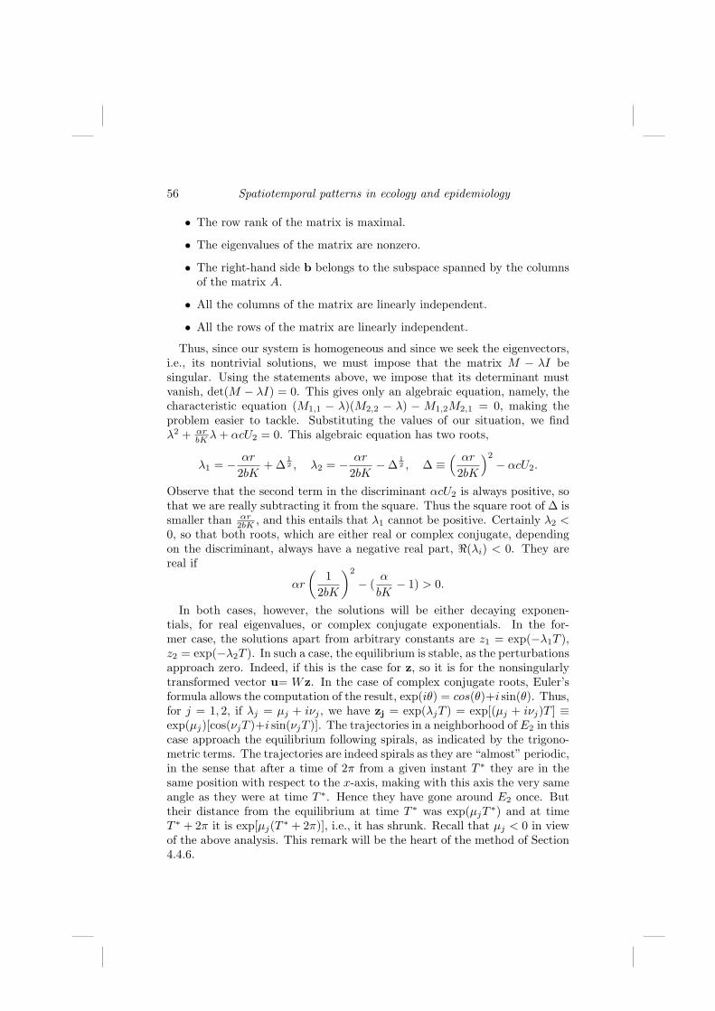
56 Spatiotemporal patterns in ecology and epidemiology
• The row rank of the matrix is maximal.
• The eigenvalues of the matrix are nonzero.
• The right-hand side b belongs to the subspace spanned by the columnsof the matrix A.
• All the columns of the matrix are linearly independent.
• All the rows of the matrix are linearly independent.
Thus, since our system is homogeneous and since we seek the eigenvectors,i.e., its nontrivial solutions, we must impose that the matrix M − λI besingular. Using the statements above, we impose that its determinant mustvanish, det(M − λI) = 0. This gives only an algebraic equation, namely, thecharacteristic equation (M1,1 − λ)(M2,2 − λ) − M1,2M2,1 = 0, making theproblem easier to tackle. Substituting the values of our situation, we findλ2 + αr
bK λ + αcU2 = 0. This algebraic equation has two roots,
λ1 = − αr
2bK+ ∆
12 , λ2 = − αr
2bK−∆
12 , ∆ ≡
( αr
2bK
)2
− αcU2.
Observe that the second term in the discriminant αcU2 is always positive, sothat we are really subtracting it from the square. Thus the square root of ∆ issmaller than αr
2bK , and this entails that λ1 cannot be positive. Certainly λ2 <0, so that both roots, which are either real or complex conjugate, dependingon the discriminant, always have a negative real part, <(λi) < 0. They arereal if
αr
(1
2bK
)2
− (α
bK− 1) > 0.
In both cases, however, the solutions will be either decaying exponen-tials, for real eigenvalues, or complex conjugate exponentials. In the for-mer case, the solutions apart from arbitrary constants are z1 = exp(−λ1T ),z2 = exp(−λ2T ). In such a case, the equilibrium is stable, as the perturbationsapproach zero. Indeed, if this is the case for z, so it is for the nonsingularlytransformed vector u= Wz. In the case of complex conjugate roots, Euler’sformula allows the computation of the result, exp(iθ) = cos(θ)+i sin(θ). Thus,for j = 1, 2, if λj = µj + iνj , we have zj = exp(λjT ) = exp[(µj + iνj)T ] ≡exp(µj)[cos(νjT )+i sin(νjT )]. The trajectories in a neighborhood of E2 in thiscase approach the equilibrium following spirals, as indicated by the trigono-metric terms. The trajectories are indeed spirals as they are “almost” periodic,in the sense that after a time of 2π from a given instant T ∗ they are in thesame position with respect to the x-axis, making with this axis the very sameangle as they were at time T ∗. Hence they have gone around E2 once. Buttheir distance from the equilibrium at time T ∗ was exp(µjT
∗) and at timeT ∗ + 2π it is exp[µj(T ∗ + 2π)], i.e., it has shrunk. Recall that µj < 0 in viewof the above analysis. This remark will be the heart of the method of Section4.4.6.
Interacting populations 57
Summarizing discussion
Implications of any model predictions should be interpreted in terms of thescience where it stems from. Let us therefore consider what we have learntfrom the above analysis. Suppose that U represents some kind of nuisancespecies that we would like to fight with biological means, i.e., using one ofits natural predators V . The problem may then be that in the environmentwhere U is present, other species appetible to V may also be present. Insuch a case, V has a choice on which species to feed upon. The interiorequilibrium we have found expresses the fact that if the carrying capacity Kfor the predators V is not high enough, they survive by feeding partly onthe other populations present and partly on U , but the latter survives in theenvironment and settles to the value U2. On the other hand, if K is raised highenough, the equilibrium moves on the V -axis, i.e., the predator will bring thepest U to extinction. Thus, in order to eliminate the latter, if we cannot actdirectly on the number of their natural predators, we could at least providethem with enough alternative food sources in order to raise their environmentcarrying capacity K so that they are then able to wipe out the pest U .
4.2 Classical Lotka–Volterra model
In contrast to the model presented earlier, the classical Lotka–Volterra con-siders an aquatic environment, in which the sharks have as their food sourcethe other fish, which all together constitute the prey. In their absence, thepredators exhibit a negative growth rate, −e. This assumption is indeed themain difference with the model of Section 4.1. In the classical model, theequations read
dU
dT= U(T )[α− bV (T )],
dV
dT= V (T ) [−e + cU(T )] . (4.8)
If one carries out the linearization procedure outlined before, about theequilibrium ( e
c , αb ) in the UV phase space, we would find in this case purely
imaginary eigenvalues λ = ±iσ, σ =√
αe, since the Jacobian and character-istic equations are now
M ≡[
0 − 1c eb
1b cα 0
]and λ2 + eα = 0,
respectively.The basis for the linearized solution is then given by exp(±σT ) = cos(σT )±
i sin(σT ). Near the equilibrium point the solution trajectories are thus closedcurves, giving the so-called neutral stability. If two different initial conditionsare considered, the trajectories starting from each one of them will return to
58 Spatiotemporal patterns in ecology and epidemiology
the initial values after a certain time. In other words, perturbing the initialvalues, the trajectories do not approach the equilibrium, they rather remainconfined to a suitable neighborhood of this point. From a practical point ofview this is not satisfactory, as biologically an equilibrium should attract orrepel trajectories and not be too sensitive to the initial conditions.
4.2.1 More on prey–predator models
Now we consider a more general model than the original Lotka–Volterramodel, with the aim of overcoming the weakness it possesses, namely, theneutral stability of its equilibrium. In order to do that, we will assume thatthe environment for the prey is no longer unlimited, that a carrying capacityexists to limit their growth. Let the prey and predator populations be againexpressed respectively by the functions U(T ) and V (T ). As for the classi-cal Lotka–Volterra system, assume the prey are the sole food source for thepredators, so that the mortality rate for the latter is exponential in absenceof the former. This is then a different environment than the one discussed inSection 4.1. The system is therefore
dU
dT= U(a− bV − eU),
dV
dT= V (−c + dU). (4.9)
The equilibria are the origin and then the points E1 = (ae , 0) and E2 ≡
(U∗, V ∗), with U∗ = cd , V ∗ = 1
bd (ad − ce). This nontrivial equilibrium pointis feasible for ad > ce. The system’s Jacobian is easily evaluated,
J =(
a− bV − 2eU −bUdV −c + dU
). (4.10)
It follows that, when feasible, E2 is also asymptotically stable, as the eigen-values of the Jacobian are
λ± = −eU∗
2±
√(eU∗
2
)2
− bdU∗V ∗ = − ce
2d± 1
2
√c2e2
d2+
4c
d(ce− ad)
and thus always have a negative real part. The point E2 is then a focus or anode, depending on whether the argument of the root is negative or positive.Both conditions can arise, as by fixing all parameters, except for the preynet birth rate, we see that for a = 0 or very small, the eigenvalues are real,thus giving a node, while for a → +∞ they become complex conjugate, andE2 would thus be a focus. Worthy of notice is also the fact that should E2
become infeasible, the boundary equilibrium E1 = (ae , 0) would then be the
new and only equilibrium. Its eigenvalues are −a, 1e (ad− ce). These entail an
important consequence, indeed that the infeasibility condition of E2 impliesE1 to be stable, and vice versa. Thus the ω-limit set of this model is givenonly by the points E2 and E1. Notice indeed that the origin is a saddle since

Interacting populations 59
the trajectories escape from it along the U -axis. Thus the community cannever become extinct, as the prey are prevented from vanishing. On the otherhand, it is possible either that both species survive at levels prescribed by E2,or that only the predators disappear, at the equilibrium E1.
4.2.2 Scaling
We want to review what was already done in the case of the one-populationmodels, to simplify the equations. In the later chapters we will appreciatethis technique, since it is powerful enough to allow substantial reduction ofthe number of parameters appearing in a system of equations. Bearing in mindthe system (4.8), let us introduce new dependent and independent variables bymeans of the equations U(T ) = Au(t), V (T ) = Bv(t), T = Ct, with A, B, Cdenoting positive constants to be determined. Taking derivatives, the chainrule yields
dU
dT= A
du
dt
dt
dT=
A
C
du
dt,
dV
dT= B
dv
dt
dt
dT=
B
C
dv
dt.
Thus back substitution into (4.8) gives
du
dt= Cu(t)[α− bBv(t)],
dv
dt= Cv(t) [−e + cAu(t)] . (4.11)
Now we want to choose the scaling constants so as to minimize the numberof parameters in the rescaled system. We can thus choose to set Cα = 1 andCbB = 1 in the first equation in (4.11), thus giving C = 1
α , B = αb . If we now
try to make use of the second equation in (4.11), setting Ce = 1, we see thatit is not possible. Thus θ = e
α is a rescaled parameter intrinsic to the model.On the contrary, we can still use the left degree of freedom by setting
CcA = 1, i.e., selecting A = αc . The rescaled model then reads
du
dt= u(t)[1− v(t)],
dv
dt= v(t) [−θ + u(t)] . (4.12)
From the simulation point of view, let us illustrate the advantage of thisprocedure. Suppose we would like to investigate the model’s behavior for arange of parameter values, saving the plots of the simulations. Fixing theoriginal parameters to some values, say b = 0.1, c = 0.1, e = 0.1, we may letthe last parameter vary in a certain range, say α = 0.1, 0.2, . . . , 0.9, 1.0, thusobtaining 10 figures. Then we need to change the value of another parameter,b = 0.2 say, and repeat the operation, obtaining another 10 figures. Repeatingagain the procedure for b = 0.3, . . . , 0.9, 1, we thus have 100 figures, which wecan arrange in a 10 by 10 table in a single page. Then we repeat the wholeconstruction for the value c = 0.2, obtaining a second “page” with another100 figures, and then a third one for c = 0.3, and so on up to c = 1.0. In thisway a “chapter” of 10 pages and 1000 figures is obtained, all corresponding
60 Spatiotemporal patterns in ecology and epidemiology
to e = 0.1. We then let e = 0.2 and again repeat the procedure, gettinga second chapter, and so on, until for e = 1.0 we have completed a bookof 10000 figures. Scaling instead allows us just to run the simulation for arange of values of the new parameter θ, so that all the behaviors of the modelcontained in the former simulations can be traced back to some of the latter,for suitable parameter combinations. Indeed, looking at the definition of θ, itis clear that the simulations for the pairs α = 0.1, e = 0.2, α = 0.3, e = 0.6and α = 0.4, e = 0.8 all correspond to the same figure in the last set obtainedfor θ = 2. The advantage in terms of computational costs and easiness ofreading the results is apparent.
4.3 Other types of population communities
Prey–predator interactions are among the most important in ecologicalcommunities, yet they of course are not the only ones possible. In this sectionwe give an overview of some other types of interspecific interactions as wellas some other and complementary modeling approaches.
4.3.1 Competing populations
Competing species can be either predators directly competing among them-selves or species that survive in the same ecosystem exploiting the same re-sources, e.g., sharing a common pasture. It is known that among wild un-gulates, direct competition for the same pastures arises between the red deer(Cervus elaphus hippelaphus) and the roe deer (Capreolus capreolus), the for-mer suffering the most as the other wild ungulates are more generalist in thehabitat selection as well as in feeding habits. The roe deer, in Mediterraneanareas, also suffers from the presence of the fallow deer (Dama dama). Anexample for exploitation of the same trophic niches, in the Gran ParadisoNational Park in the Northwestern Alps in Italy, is given by goats and thewild chamois (Rupicapra rupicapra) and ibex (Capra ibex). Another instanceinvolves skuas and seagulls populations, which compete for food, since theirtrophic niches overlap. Skuas (Stercorarius spp.) predates on seagulls’ new-borns, while the seagulls predate on eggs of the other species. In the NationalPark of the Tuscan Islands, in the Tirrenian Sea, competion for nidificationoccurs among seagulls (Larus audouinii and Larus cacchinnans). Moreover,the latter predates upon newborns and adults of the former.
To model situations of this type, let the population sizes be denoted P (T )and Q (T ). The classical competition model then reads
dP
dT= P [a− bP − cQ] ,
dQ
dT= Q [d− eP − fQ] . (4.13)
Interacting populations 61
Each equation states the logistic reproduction of the corresponding species,and its negative interaction with the other one is expressed by the negativesign of the mixed term. The equilibria analysis for (4.13) shows that thenullcline for P intersects the coordinate axes at P ≡ P1 = a
b and Q = ac , and
the one for Q intersects them at P = de and Q = d
f .Since for very small values of both populations the dominant terms in (4.13)
are the positive constants, it is immeditely found that the equilibrium locatedat the origin E0 ≡ (P0, Q0) ≡ (0, 0) is unstable, while the equilibrium E1 ≡(P1, Q1) ≡
(P , 0
) ≡ (ab , 0
)is conditionally stable, namely, if the condition
P < P holds, i.e.,bd < ae. (4.14)
For E2 ≡ (P2, Q2) ≡(0, Q
) ≡(0, d
f
)stability holds for Q < Q, i.e.,
af < cd. (4.15)
The nontrivial equilibrium E3 ≡ (P3, Q3) ≡(
af−cdbf−ce , bd−ae
bf−ce
)exists if the
two nullclines intersect each other, which happens if the condition bf 6= ceis satisfied. But this intersection has to lie in the first quadrant, and thecondition under which this nontrivial equilibrium is feasible then becomes therequirement that bf − ce, bd− ae, and af − cd all possess the same sign, i.e.,either one of the following alternative statements holds:
b
e>
a
d>
c
f, i.e. P > P , Q > Q and sl
(P Q
)< sl
(P Q
), (4.16)
b
e<
a
d<
c
f, i.e. P < P , Q < Q and sl
(P Q
)< sl
(P Q
), (4.17)
where “sl” stands for the slope.The Jacobian of the system is
J =(
a− 2bP − cQ −cP−eQ d− eP − 2fQ
). (4.18)
The eigenvalues at E3 are then easily found,
λ1,2 =12
α±√∆bf − ce
, α = −b (af − cd)− f (bd− ae) , (4.19)
∆ = α2 − 4 (af − cd) (bd− ae) (bf − ce) .
The feasibility conditions (4.16) imply that
α
bf − ce≡ −bP3 − fQ3 < 0,
from which it follows that at least one of the eigenvalues is necessarily negative.From (4.16) it follows that ∆ < α2, so that λ2 ≡ 1
bf−ce
(α +
√∆
)< 0. In

62 Spatiotemporal patterns in ecology and epidemiology
such a case, the equilibrium E3 is stable and the whole ecosystem thrives,with both populations at nonzero level. Since only one eigenvalue can bemade positive, upon destabilization of E3 we would get a saddle. For this tooccur, we need the conditions (4.17). It then follows that the saddle impliesthe existence through it of a separatrix in the phase plane, dividing it intobasins of attraction, one each for the remaining equilibria E1 and E2, whichare then mutually exclusive. Thus only one of the two species survives, whilethe other one becomes extinct. As to which is which, the answer depends onthe initial condition of the system. Trajectories emanating from a point inthe basin of the equilibrium E1 where only the P ’s thrive tend asymptoticallyto this point, thus wiping out the Q population, and vice versa.
The Russian biologist Gause in his famous laboratory experiments has de-termined the evolution of two species of yeast, the P population of Saccha-romyces cerevisiae and the Q population of Schizosaccharomyces kefyr. Whenliving independently from each other (cf. Renshaw, 1991), he found the fol-lowing growth laws:
P =13
1 + e3.32816−0.21827t, Q =
5.81 + e2.47550−006069t
.
When allowed to interact, however, the two species became competitors andtheir evolution would follow the empirical findings
dP
dT= rP P (1− SPP P − SPQQ),
dQ
dT= rQQ(1− SQQQ− SQP P ),
where
rP = 0.21827, sPP = 0.01679, sPQ = 3.15× SPP = 0.05289rQ = 0.06069, sQQ = 0.01046, sQP = 0.439× SQQ = 0.00459 .
4.3.2 Symbiotic populations
Some scientists argue that symbiotic communities do not develop easilyin ecological time, but rather represent evolutionary interactions. Therefore,population models to take this into account should contain different timescales. However, their remark may be easily questioned by considering one ofthe most elementary facts in nature, namely, the role that insects, in particularbees, have in the fecundation of flowers (e.g., see Boucher, 1985, p. 85). Anentire chapter is devoted to this topic in Boucher (1985, p. 145), which containsa discussion of some aspects of evolution in a mutualistic environment.
Other well-known mutualistic interactions in nature are found in a wealthof different enviroments, such as in diatom mats in the ocean, between man-groves and root borers, spiders and parasitic wasps, invertebrates and theirepibionts, and corals and fish. These as well as many other examples are
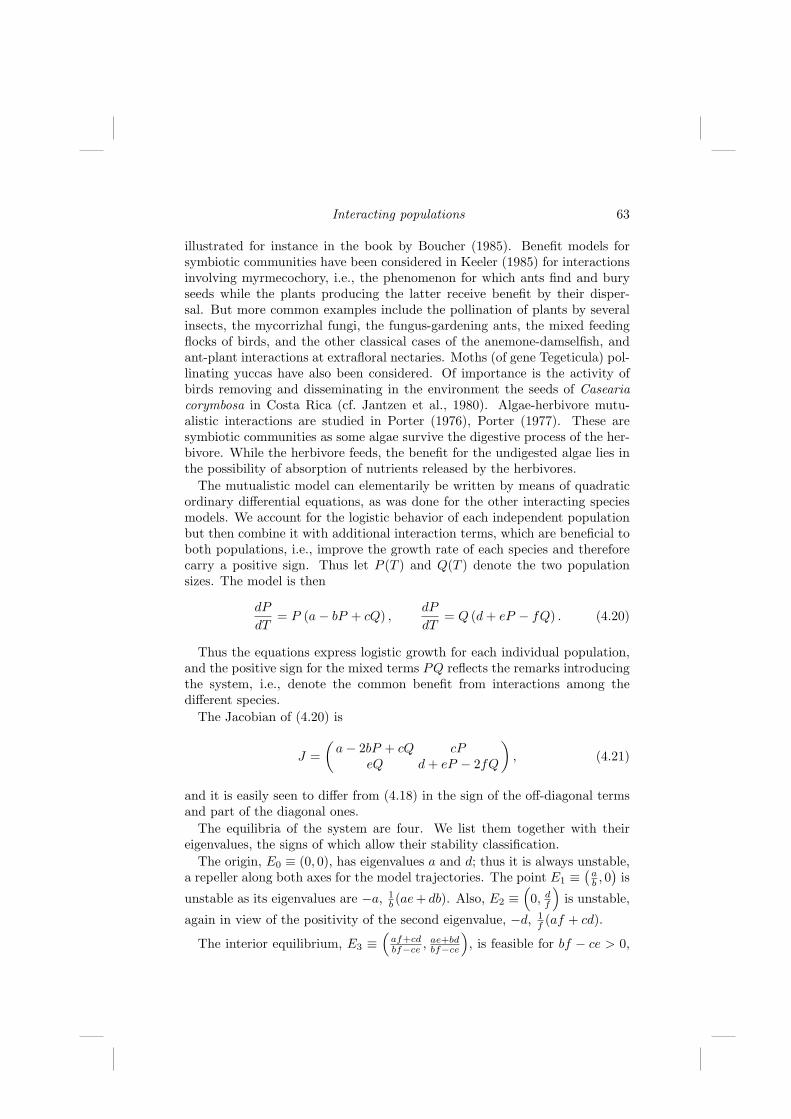
Interacting populations 63
illustrated for instance in the book by Boucher (1985). Benefit models forsymbiotic communities have been considered in Keeler (1985) for interactionsinvolving myrmecochory, i.e., the phenomenon for which ants find and buryseeds while the plants producing the latter receive benefit by their disper-sal. But more common examples include the pollination of plants by severalinsects, the mycorrizhal fungi, the fungus-gardening ants, the mixed feedingflocks of birds, and the other classical cases of the anemone-damselfish, andant-plant interactions at extrafloral nectaries. Moths (of gene Tegeticula) pol-linating yuccas have also been considered. Of importance is the activity ofbirds removing and disseminating in the environment the seeds of Caseariacorymbosa in Costa Rica (cf. Jantzen et al., 1980). Algae-herbivore mutu-alistic interactions are studied in Porter (1976), Porter (1977). These aresymbiotic communities as some algae survive the digestive process of the her-bivore. While the herbivore feeds, the benefit for the undigested algae lies inthe possibility of absorption of nutrients released by the herbivores.
The mutualistic model can elementarily be written by means of quadraticordinary differential equations, as was done for the other interacting speciesmodels. We account for the logistic behavior of each independent populationbut then combine it with additional interaction terms, which are beneficial toboth populations, i.e., improve the growth rate of each species and thereforecarry a positive sign. Thus let P (T ) and Q(T ) denote the two populationsizes. The model is then
dP
dT= P (a− bP + cQ) ,
dP
dT= Q (d + eP − fQ) . (4.20)
Thus the equations express logistic growth for each individual population,and the positive sign for the mixed terms PQ reflects the remarks introducingthe system, i.e., denote the common benefit from interactions among thedifferent species.
The Jacobian of (4.20) is
J =(
a− 2bP + cQ cPeQ d + eP − 2fQ
), (4.21)
and it is easily seen to differ from (4.18) in the sign of the off-diagonal termsand part of the diagonal ones.
The equilibria of the system are four. We list them together with theireigenvalues, the signs of which allow their stability classification.
The origin, E0 ≡ (0, 0), has eigenvalues a and d; thus it is always unstable,a repeller along both axes for the model trajectories. The point E1 ≡
(ab , 0
)is
unstable as its eigenvalues are −a, 1b (ae + db). Also, E2 ≡
(0, d
f
)is unstable,
again in view of the positivity of the second eigenvalue, −d, 1f (af + cd).
The interior equilibrium, E3 ≡(
af+cdbf−ce , ae+bd
bf−ce
), is feasible for bf − ce > 0,

64 Spatiotemporal patterns in ecology and epidemiology
and it has the eigenvalues
λ(d)3,± ≡
12
− (bP3 + fQ3)±
[(bP3 + fQ3)
2 − 4 (bf − ce) P3Q3
] 12
. (4.22)
Hence, in view of the feasibility condition, the real parts of the eigenvaluesare negative, thus always providing stability. As no other point is stable,the model dynamics must then be drawn to this equilibrium, which is thenglobally asymptotically stable. Furthermore, at the level provided by E3,survival of both species is at a higher level than the one specified by theequilibrium for each single species, this being the heart of mutualism. ThusE3 is more favorable than the equilibria provided by the carrying capacityof each species, and which each population would enjoy in the absence of itssymbiotic counterpart. Finally, for bf < ce, the ω-limit set of the system isthe point at ∞, i.e., all trajectories would tend to larger and larger valuesfor both P and Q. We would thus have an “explosion” of the populations,when E3 becomes infeasible. On the other hand, it is easy to show that thetrajectories are bounded if the feasibility condition for the interior equilibriumis satisfied, namely, bf > ce. It is enough to sketch the two nullclines in thephase plane and afterwards analyze the sign of the flow to show that it wouldpoint “inwards” toward the origin on any curve whose points (P,Q) cut aset in the first quadrant containing O and E3 and lie enough away from theorigin.
4.3.3 Leslie–Gower model
As usual, we denote by U(T ) and V (T ) respectively the prey and predatorsizes. The Leslie–Gower classical model assumes that when predation is notconsidered the prey population exhibits logistic growth, so that there arelimited resources in the environment, leading to a carrying capacity K and netbirth rate r. The basic feature of the Leslie–Gower model is the assumptionthat the predator’s carrying capacity is variable, and in particular proportionalto the prey size. The proportionality constant h indicates the prey amountneeded to feed a predator in equilibrium conditions:
dU
dT= rU
(1− U
K
)− cUV,
dV
dT= aV
(1− h
V
U
). (4.23)
In adimensional form, it becomes
du
dt= u(1− u− v),
dv
dt= v
(δ − β
v
u
), δ =
a
r, β =
ah
cK2r. (4.24)
The full analysis of this system can be found in Hsu and Huang (1995). Noteonly that there are two equilibria, E∗ ≡ (1, 0) and E† ≡ (u† ≡ β
β+δ , v† ≡ δβ+δ ).
The Jacobian is
J =(
1− 2u− v −u
β v2
u2 δ − 2β vu
). (4.25)

Interacting populations 65
At E∗, the eigenvalues are easily seen to be −1, δ so that this equilibrium isalways unstable. At E†, the characteristic equation is λ2 + (δ + u†)λ + δ = 0and gives the eigenvalues
λ± =12
[−δ − u† ±
√(δ + u†)2 − δ
]
so that λ± < 0 always, thus E† is a stable equilibrium. It is a focus ifδ2 + (2u† − 1)δ + (u†)2 < 0, which then implies 1 − 2u† −
√1− 4u† < δ <
1− 2u† +√
1− 4u†, and conversely it would be a node.
4.3.4 Classical Holling–Tanner model
The Holling–Tanner model for the prey–predator interaction assumes thesame dynamics of the Leslie–Gower model for both species, except that thecapturing term on prey is replaced by a saturation function f(U, V ), i.e.,a function with a horizontal asymptote, May (1973), Renshaw (1991), andTanner (1975). Models for it could be, for instance,
f(U, V ) =m
A + UUV, f(U, V ) = mV (1− eαU ).
In this case we consider the Holling type II functional response. The modelis then
dU
dT= rU
(1− U
K
)− m
A + UUV,
dV
dT= V γ
(1− h
V
U
). (4.26)
A nondimensional form of system (4.26) can be obtained by setting
u ≡ 1K
U, v ≡ m
rKV, t ≡ rT, δ ≡ γ
r, β ≡ γh
m, a ≡ A
K,
so that we get
du
dt= u(1− u)− 1
a + uuv,
dv
dt= v
(δ − β
v
u
). (4.27)
These can be studied geometrically as follows. The isoclines give respectivelya parabola and a straight line through the origin
du
dt= 0 : v = (a + u)(1− v);
dv
dt= 0 : v =
δ
βu. (4.28)
The parabola has the vertex at (u, v), u = 12 (1−a), v = 1
4r(1 + a)2, and it haspositive height a at the origin and a feasible root at u0 = 1. On geometricalgrounds, an intersection in the first quadrant always exists, so that a feasibleequilibrium is always guaranteed. In fact, for (4.27), we also find the boundaryequilibria O and E1(1, 0) in addition to the interior one E2(u∗, v∗) with
u∗ =12
[D +
√D2 + 4a
], D = 1− a− δ
β, v∗ = u∗
δ
β. (4.29)
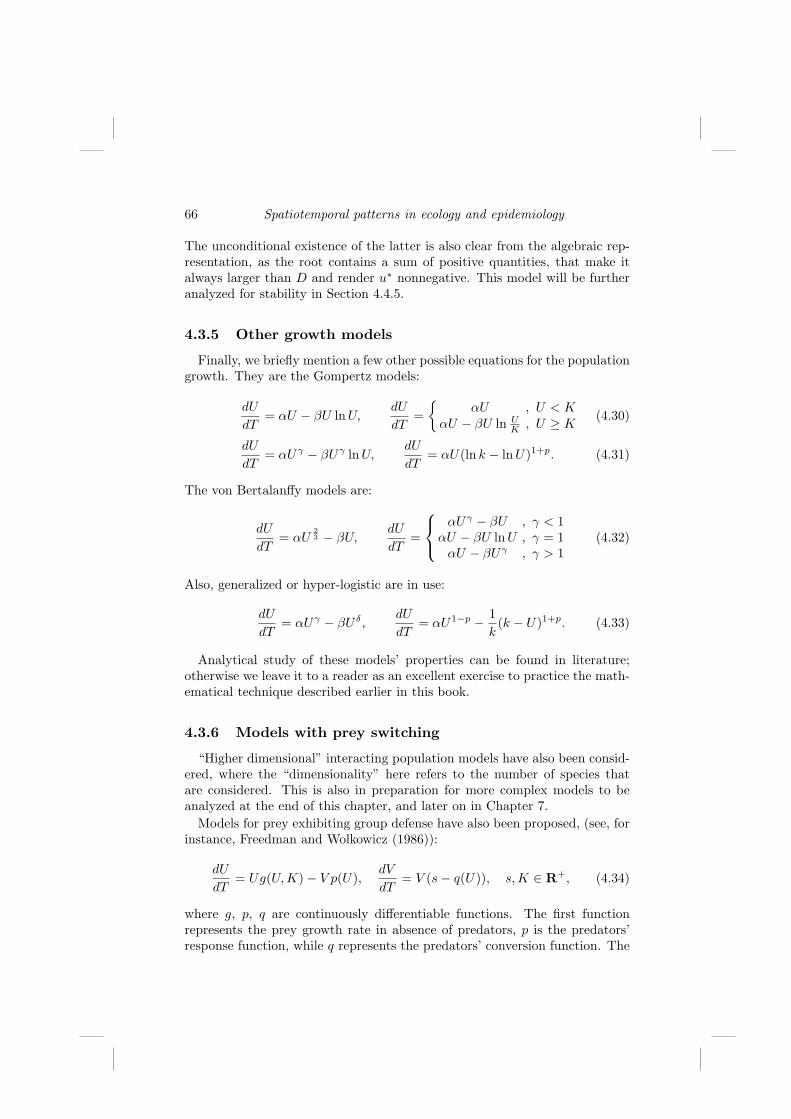
66 Spatiotemporal patterns in ecology and epidemiology
The unconditional existence of the latter is also clear from the algebraic rep-resentation, as the root contains a sum of positive quantities, that make italways larger than D and render u∗ nonnegative. This model will be furtheranalyzed for stability in Section 4.4.5.
4.3.5 Other growth models
Finally, we briefly mention a few other possible equations for the populationgrowth. They are the Gompertz models:
dU
dT= αU − βU ln U,
dU
dT=
αU , U < K
αU − βU ln UK , U ≥ K
(4.30)
dU
dT= αUγ − βUγ ln U,
dU
dT= αU(ln k − ln U)1+p. (4.31)
The von Bertalanffy models are:
dU
dT= αU
23 − βU,
dU
dT=
αUγ − βU , γ < 1αU − βU ln U , γ = 1
αU − βUγ , γ > 1(4.32)
Also, generalized or hyper-logistic are in use:
dU
dT= αUγ − βU δ,
dU
dT= αU1−p − 1
k(k − U)1+p. (4.33)
Analytical study of these models’ properties can be found in literature;otherwise we leave it to a reader as an excellent exercise to practice the math-ematical technique described earlier in this book.
4.3.6 Models with prey switching
“Higher dimensional” interacting population models have also been consid-ered, where the “dimensionality” here refers to the number of species thatare considered. This is also in preparation for more complex models to beanalyzed at the end of this chapter, and later on in Chapter 7.
Models for prey exhibiting group defense have also been proposed, (see, forinstance, Freedman and Wolkowicz (1986)):
dU
dT= Ug(U,K)− V p(U),
dV
dT= V (s− q(U)), s, K ∈ R+, (4.34)
where g, p, q are continuously differentiable functions. The first functionrepresents the prey growth rate in absence of predators, p is the predators’response function, while q represents the predators’ conversion function. The

Interacting populations 67
assumptions they obey are summarized as follows:
g(0,K) = g(K, K) = 0,
∂g
∂U(K,K) < 0,
∂g
∂U(U,K) ≤ 0,
∂g
∂K(U,K) > 0,
p(0) = 0, p(U) ≥ 0,
dp
dU> 0 for 0 ≤ U < M,
dp
dU< 0 for U > M,
q(0) = 0, q(U) ≥ 0, q(M) > s,
dq
dU> 0 for 0 ≤ U < M,
dq
dU< 0 for U > M,
where M > 0 denotes a suitable constant.A model incorporating group defense in a community dwelling in a frag-
mented habitat was developed by Khan et al. (1998):
dU1
dT= (α1 − ε1)U1 + ε2p21U2 − β1U
22 V
U1 + U2, (4.35)
dU2
dT= (α2 − ε2)U2 + ε1p12U1 − β2U
21 V
U1 + U2,
dV
dT= V
(−ν +
δ1β1U22
U1 + U2+
δ2β2U21
U1 + U2
),
where U1 and U2 denote the prey species living in the two separate habitats.The parameters are interpreted as follows. The predator response rates towardeach species of prey are βi, i = 1, 2; their respective conversion rates are δi;εi denotes the inverse barrier strengths going out of habitat i; and pi,j isthe probability of such a successful move. The specific growth rate of theprey when predators are absent is αi, and ν is the per capita death rate ofpredators.
Khan et al. (2002) also developed a model that incorporates a stage struc-ture in addition to switching:
dU1
dT= βU2 − µ1U1 − βU2(T − τ)e−µ1τ − b1U
21 V
U1 + U2+ hU1U2, (4.36)
dU2
dT= βU2(T − τ)e−µ1τ − µ2U
22 −
b1U22 V
U1 + U2+ gU1U2,
dV
dT= V
(c1β1U
21
U1 + U2+
c2β2U22
U1 + U2− d
)
(see also McNair, 1987), with U1 and U2 denoting the immature and adultpopulations, τ representing the time from birth to reach maturity, the termβU2(T − τ)e−µ1τ expressing the fraction of young individuals who reach the

68 Spatiotemporal patterns in ecology and epidemiology
maturity stage, and gU1U2 and hU1U2 are interaction terms. The parametershave the following meanings: β is the per capita birth rate of the prey speciesin stage 2, γ is the maturation rate from stage 1 to stage 2, µi is the percapita death rate, bi is the capture rate of prey species of stage i, ci is theconversion factor for prey species of stage i, and d is the per capita death rateof the predator.
Another switching similar model is presented in Tansky (1978):
dU1
dT= U1
E1 − aV
1 +(
U2U1
)n
, (4.37)
dU2
dT= U2
E2 − bV
1 +(
U1U2
)n
,
dV
dT= V
−E3 +
aU1
1 +(
U2U1
)n +bU2
1 +(
U1U2
)n
,
where the positive integer n is a parameter.A similar model was also considered by Khan et al. (2004):
dU1
dT= g1U1
(1− U1
K1
)+ e2p21U2 − β1U1U2V
U1 + U2, (4.38)
dU2
dT= g2U2
(1− U2
K2
)+ e1p12U1 − β2U1U2V
U1 + U2,
dV
dT= V
(−µ +
(δ1β1 + δ2β2)U1U2
U1 + U2
),
where Ki represents the carrying capacity of each prey; gi is the net effect ofbirth, death and migration rates; and the remaining parameters have inter-pretations as above, (4.36), namely, ei and pij represent the strength of thebarrier and the probability of moving to a different habitat, βi the predatorresponses to each prey, δi the conversion factors, and µ the per capita deathrate of predators.
4.4 Global stability
Let us consider again the classical Lotka–Volterra system,
dU
dT= U(a− bV ),
dV
dT= V (−m + cU). (4.39)

Interacting populations 69
In an attempt to find a closed form solution, we can calculate the slope ofthe trajectories in the UV phase plane. Using the chain rule and exploiting(4.39), we get
dV
dU=
dV
dT×
[dU
dT
]−1
=V (−m + cU)U(a− bV )
,
so that variables can be separated to yield∫
(a− bV )dV
V=
∫(−m + cU)
dU
U; a ln V − bV = −m ln U + cU − h.
Therefore we can introduce the function
z = L(U, V ) ≡ −a ln V + bV −m ln U + cU − h, (4.40)
which represents a surface defined on the phase space. The orbits of the model(4.39) are the loci of points (U, V ) in the phase space for which L(U, V ) = hfor the constant h ∈ R, i.e., the level curves z = h of the surface z = L(U, V );the larger h is, the higher these levels are. In particular, given the initialcondition (U0, V0), the solution of the initial value problem is the level curveof L = h0, where h0 corresponds to
h0 = −a ln V0 + bV0 −m ln U0 + cU0. (4.41)
To further study L, it is immediately seen that ∇L = 0 at the equilibriumpoint of the system (4.39), E∞ ≡ (U∞, V∞) with U∞ = m
c , V∞ = ab , and from
this we define the value of the constant there as
h∞ = −a ln V∞ + bV∞ −m ln U∞ + cU∞ (4.42)
= a(1− ln
a
b
)+ m
(1− ln
m
c
).
The shape of the surface can be investigated by intersecting it with verticalplanes. On V = V , we easily find that L → +∞ both when U → +∞ aswell as U → 0+. Similarly, on U = U , we have L → +∞ for V → 0+
and V → +∞. It appears that the equilibrium E∞ is then a minimum. Tofurther support this statement, we consider the intersection with a genericplane V = rU + s. Then
L(U) ≡ L(U, V ) ≡ −m ln U + cU − a ln(rU + s) + b(rU + s)
and we must distinguish several cases. For r, s > 0, as U → +∞ we have
L = U
[c−m
ln U
U
]+ (rU + s)
[b− a
ln(rU + s)rU + s
]→ +∞.
The behavior L → +∞ can also be discovered for U → +∞ in the other cases.The function indeed needs to be investigated also on the remaining parts of

70 Spatiotemporal patterns in ecology and epidemiology
the boundary of its domain, which is R+ ×R+ = (U, V ) : U > 0, ; V > 0.By taking the other suitable limits, namely, for r, s > 0 as U → 0+, while forr > 0, s < 0 as V ≡ rU + s → 0+, we find again L → ∞. The case r < 0,s > 0 needs more care as the limits at infinity cannot be taken; rather, we mustevaluate L when both U → 0+ and rU + s → 0+, but again the conclusionis L → ∞. The surface L thus appears to be a bowl, going up vertically onthe coordinate axes and also growing as the points in the domain drift towardinfinity. E∞ then appears to be its absolute minimum. To mathematicallysubstantiate this claim, we can compute the Hessian matrix,
HL =∣∣∣∣mU−2 0
0 aV −2
∣∣∣∣ > 0,
to discover that the curvature of the surface is always positive, i.e., the surfaceis everywhere convex. Therefore E∞ really represents an absolute minimum.By (4.40) and (4.42) we would then have L(E∞) = 0. This is the first propertyof the Lyapunov function. We have also shown that L(U, V ) ≥ L(E∞) = 0,which constitutes its second property. Below we will discover finally its thirdand fundamental property, namely, that the system trajectories enter into thisbowl. In the present case, calculating the tangential derivative of L we findthat it is tangent to the solution trajectories,
dL
dT=
∂L
∂U
dU
dT+
∂L
∂V
dV
dT= −m
UU(a− bV ) + cU(a− bV )
− a
VV (−m + cU) + bV (−m + cU) = 0.
The function L also allows the explicit analytical determination of the or-bits. To this end, using the initial condition (4.41) coupled with the definition(4.40) of L, we have
−m(lnU − ln U0) + c(U − U0) = a(lnV − ln V0)− b(V − V0)
from which
c(U − U0) + b(V − V0) = ln(
V
V0
)a
+ ln(
U
U0
)m
and finally the closed forms of the orbits(
U
U0
)m (V
V0
)a
= ec(U−U0)+b(V−V0).
To investigate further the latter, let us study small perturbations around theequilibrium, by defining u = U−U∞ = U−m
c ∈ R, v = V −V∞ = V − ab ∈ R.
Substitution into L(U, V ) = h brings
− m[ln
m
c+ ln
(1 +
cu
m
)]+ m
(1 +
cu
m
)
− a
[ln
a
b+ ln
(1 +
bv
a
)]+ a
(1 +
bv
a
)= h.

Interacting populations 71
Now, using Taylor’s formula and keeping only terms up to the second order,we are led to
− m
[ln
m
c+
cu
m− 1
2
(cu
m
)2]
+ m(1 +
cu
m
)
− a
[ln
a
b+
bv
a− 1
2
(bv
a
)2]
+ a
(1 +
bv
a
)= h.
Linearization and further simplifications give
m
2
(cu
m
)2
+a
2
(bv
a
)2
= −m− a + h + m lnm
c+ a ln
a
b
and, finally, using (4.42) we arrive at
u2
A2+
v2
B2= H, A2 =
2mc2
, B2 =2a
b2, H = h− h∞ ≥ 0.
The trajectories around the equilibrium are therefore close to ellipses.
4.4.1 General quadratic prey–predator system
We consider now the prey–predator interactions with logistic growth in theprey, and competition among the predators, which do not have other foodsources:
dU
dT= U(a− bV − U
K1),
dV
dT= V (−m + cU − V
K2), (4.43)
with nonboundary equilibrium at E∗ = (U∗, V ∗), where
U∗ ≡ K1a + mbK2
1 + bcK1K2, V ∗ ≡ K2
−m + acK1
1 + K1bcK2,
feasible for acK1 > m. Let us consider once again the perturbations u =U − U∗, v = V − V ∗ and proceed as follows:
du
dv= −u + U∗
v + V ∗K2
K1
u + bvK1
cK2u− v,
du
u + U∗cK2u− v
K2= − dv
v + V ∗u + bvK1
K1,
which is a separable equation,
cdu− cU∗ du
u + U∗ −v
K2
du
u + U∗ = − u
K1
dv
v + V ∗ − bdv + bV ∗ dv
v + V ∗ ,
which upon integration gives
cu−cU∗ lnu + U∗
U∗ − v
K2ln(u+U∗) = − u
K1ln(v+V ∗)−bv+bV ∗ ln
v + V ∗
V ∗ +C,

72 Spatiotemporal patterns in ecology and epidemiology
where the term C represents the constant of integration. This expressionsuggests to define the following Lyapunov function:
L(u, v) ≡ cU∗[ u
U∗ − ln(1 +
u
U∗
)]+ bV ∗
[ v
V ∗ − ln(1 +
v
V ∗
)].
The property of the logarithm, x ≥ ln(1 + x) for any x > 0, implies thatL(u, v) ≥ 0, with L(0, 0) = 0. This of course corresponds to the vanishing ofL at the equilibrium point in the original coordinates. Finally,
∇L(u, v) ≡(
c− cU∗ U∗
u + U∗1
U∗ , b− bV ∗ V ∗
v + V ∗1
V ∗
)T
=(
cu
u + U∗ ,bv
v + V ∗
)T
.
It thus follows that the directional derivative along the solution trajectoriesof (4.43) is
dL
dT= ∇L · ( du
dT,dv
dT)T =
cu
u + U∗ (u + U∗)(−bv − u
K1)
+bv
v + V ∗ (v + V ∗)(+cu− v
K2)
= − 1K1
cu2 − 1K2
bv2 < 0.
This result thus shows that the trajectories make an obtuse angle with the(outward) normal to the level surfaces L(u, v) = h, i.e., they enter into thebowl defined by the Lyapunov function independently of their initial values,i.e., the equilibrium E∗ is indeed a global attractor of the system (4.43).
4.4.2 Mathematical tools for analyzing limit cycles
Here we want to mention some results in planar dynamical systems thatare useful in the investigation of solutions’ sustained oscillations; see Hirschand Smale (1974) and Strogatz (1994).
Poincare–Bendixson theorem
A closed orbit Γ of a planar dynamical system is a nonempty subset of thephase plane, Γ ⊂ R2, not containing equilibrium points.
The Poincare–Bendixson theorem states that if Γ ⊂ R2 is a closed andbounded set, and dx
dT = f(x) ∈ C1(R2) is a vector field defined on an openset containing Γ, if Γ does not contain equilibrium points, and if there is atrajectory L ⊂ Γ contained in the orbit, then L is a closed orbit or tends to aclosed orbit (i.e., a limit cycle). In other words, in such conditions Γ containsat least a limit cycle.

Interacting populations 73
The theorem can be exploited by determining a positively invariant set Ωfor the dynamical system, i.e., such that the system trajectories can only enterinto Ω, and then if possible trying to destabilize the equilibria that are foundinside Ω. The application of the above theorem would then show that at leasta stable limit cycle exists around the equilibrium.
Dulac’s criterion
The next criterion is negative, in the sense that if satisfied it shows thatlimit cycles do not exist; see Strogatz (1994). It is essentially a consequenceof Green’s theorem.
Let A ⊂ R2 be a simply connected region in the plane, i.e., it does notcontain holes, and let f and g be continuously differentiable functions in A,i.e., mathematically f, g ∈ C1(A). Given the system
dx
dT= f(x, y),
dy
dT= g(x, y), (4.44)
if a function β(x, y) ∈ C1(R2) exists for which the function
∂
∂x[β(x, y)f(x, y)] +
∂
∂y[β(x, y)g(x, y)]
is of one sign in A, then in A no closed orbit can exist.In general this result is utilized by taking A ≡ R2 and β(x, y) = (xy)−1.
As an example, let us consider the quadratic competition model
dU
dT= αU
(1− U
K
)− aUV,
dV
dT= rV
(1− V
H
)− bUV.
With the above choice for β we find
∂
∂U
1
UV
[αU
(1− U
K
)− aUV
]+
∂
∂V
1
UV
[rV
(1− V
H
)− bUV
]
= − α
KV− r
HU< 0.
It follows then that quadratic competition models do not possess limit cy-cles, and this fact clearly stems from the logistic terms in the equations, theonly ones surviving after the above differentiation.
Potential systems
A related negative result (Strogatz, 1994) states that for potential systems,limit cycles do not exist; in other words, if a function Z(x) exists for whichthe field f(x) is the gradient of Z, f(x) = ∇Z(x), i.e., Z is a potential functionfor the field, then no limit cycle for the dynamical system can exist.

74 Spatiotemporal patterns in ecology and epidemiology
As an example let us consider two logistically growing and not interactingpopulations,
dU
dT= αU
(1− U
K
),
dV
dT= rV
(1− V
H
).
Considering
Z(U, V ) =α
2U2 − α
3KU3 +
r
2V 2 − r
3HV 3 ,
the above condition is immediately verified. Of course each population evolvesnaturally toward its own carrying capacity undisturbed by the other one,these equilibria being stable in view of the results on the single-populationmodels, and in the two-dimensional phase plane the corresponding equilibriummust be stable. The corresponding Jacobian is a diagonal matrix that whenevaluated at the equilibrium (K, H), has negative entries, namely, J(K,H) =diag(−α,−r).
4.4.3 Routh–Hurwitz conditions
Stability of an equilibrium in dynamical systems as seen earlier is relatedto the negative sign of its eigenvalues, if real, or of their real part if complex.A criterion to determine the signs of the roots of a polynomial equation is theRouth–Hurwitz criterion. Namely, for the following polynomial equation therelated determinants are defined:
n∑
i=0
aiλi = 0, D1 = an−1, D2 =
∣∣∣∣an−1 an−3
an an−2
∣∣∣∣ , (4.45)
D3 =
∣∣∣∣∣∣
an−1 an−3 an−5
an an−2 an−4
0 an−1 an−3
∣∣∣∣∣∣, . . . , Dn =
∣∣∣∣∣∣∣∣∣∣
an−1 an−3 an−5 ... 0 0an an−2 an−4 ... 0 00 an−1 an−3 . . . 0 0
. . .0 0 0 . . . 0 a0
∣∣∣∣∣∣∣∣∣∣
,
with the clear understanding that aj ≡ 0 for j < 0 or j > n. The criterionstates that all the roots have negative real parts if and only if all the Dj ’s arepositive.
There is a variant of the above criterion, the Lienard–Chipart criterion,which essentially states that for stability if all coefficients are positive, ai > 0for i = 0, . . . , n, only the determinants Dn−1, Dn−3, Dn−5, . . . need to bepositive.
It is useful to see what the above statements amount to for polynomials upto degree 4. Observe that by a change of sign of the whole polynomial, theassumption an > 0 can always be made. Then, for a linear polynomial withroot λ1, trivially we need only
D1 = a0 > 0, λ = −a0
a1< 0. (4.46)
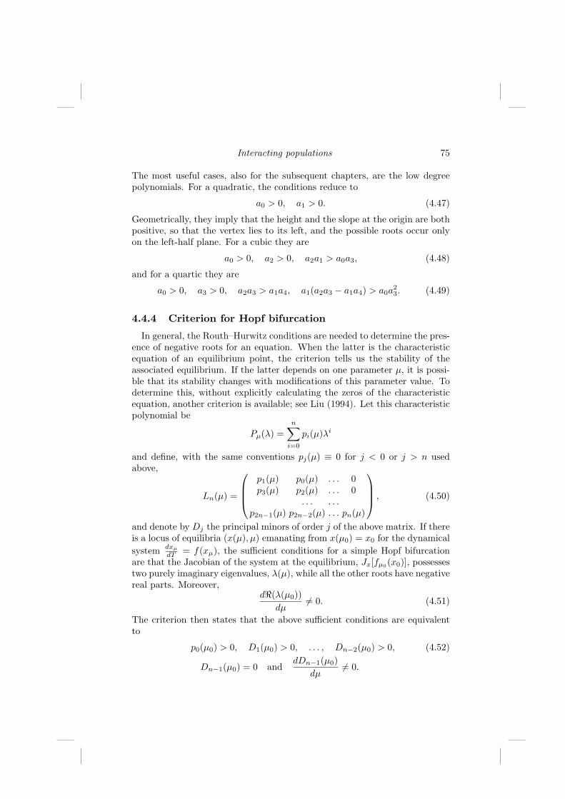
Interacting populations 75
The most useful cases, also for the subsequent chapters, are the low degreepolynomials. For a quadratic, the conditions reduce to
a0 > 0, a1 > 0. (4.47)
Geometrically, they imply that the height and the slope at the origin are bothpositive, so that the vertex lies to its left, and the possible roots occur onlyon the left-half plane. For a cubic they are
a0 > 0, a2 > 0, a2a1 > a0a3, (4.48)
and for a quartic they are
a0 > 0, a3 > 0, a2a3 > a1a4, a1(a2a3 − a1a4) > a0a23. (4.49)
4.4.4 Criterion for Hopf bifurcation
In general, the Routh–Hurwitz conditions are needed to determine the pres-ence of negative roots for an equation. When the latter is the characteristicequation of an equilibrium point, the criterion tells us the stability of theassociated equilibrium. If the latter depends on one parameter µ, it is possi-ble that its stability changes with modifications of this parameter value. Todetermine this, without explicitly calculating the zeros of the characteristicequation, another criterion is available; see Liu (1994). Let this characteristicpolynomial be
Pµ(λ) =n∑
i=0
pi(µ)λi
and define, with the same conventions pj(µ) ≡ 0 for j < 0 or j > n usedabove,
Ln(µ) =
p1(µ) p0(µ) . . . 0p3(µ) p2(µ) . . . 0
. . . . . .p2n−1(µ) p2n−2(µ) . . . pn(µ)
, (4.50)
and denote by Dj the principal minors of order j of the above matrix. If thereis a locus of equilibria (x(µ), µ) emanating from x(µ0) = x0 for the dynamicalsystem dxµ
dT = f(xµ), the sufficient conditions for a simple Hopf bifurcationare that the Jacobian of the system at the equilibrium, Jx[fµ0(x0)], possessestwo purely imaginary eigenvalues, λ(µ), while all the other roots have negativereal parts. Moreover,
d<(λ(µ0))dµ
6= 0. (4.51)
The criterion then states that the above sufficient conditions are equivalentto
p0(µ0) > 0, D1(µ0) > 0, . . . , Dn−2(µ0) > 0, (4.52)
Dn−1(µ0) = 0 anddDn−1(µ0)
dµ6= 0.

76 Spatiotemporal patterns in ecology and epidemiology
4.4.5 Instructive example
As an example of the above techniques, we consider again the Holling–Tanner model introduced in Section 4.3.4. The Jacobian in this case is
J =
(1− 2u− av 1
(a+u)2 −u 1a+u
β v2
u2 δ − 2β vu
). (4.53)
The origin and E1 are easily seen to be always unstable, having at leasta positive eigenvalue. Using (4.29), the Jacobian at the equilibrium E2 =(u∗, v∗) can be rewritten as
J∗ =
(u∗
a+u∗
(δβ −
√D2 + 4a
)−u∗ 1
a+u∗
β δ2
β −δ
). (4.54)
The Routh–Hurwitz criterion for the quadratic characteristic equation (4.47)in this case requires −Tr(J∗) > 0 and det(J∗) > 0. Easily, we find
det(J∗) =u∗δ
√D2 + 4a
a + u∗> 0.
Moreover, for the trace of the above matrix, using again (4.29), we must have
−Tr(J∗) =u∗
a + u∗
(√D2 + 4a− δ
β
)+ δ > 0. (4.55)
If the abscissa of the equilibrium lies to the right of the abscissa of the vertexof the parabola (4.28), namely, u∗ > u, i.e.
√D2 + 4a − δ
β > 2a, then (4.55)holds and E2 is then stable. For u∗ < u instead the condition (4.55) must bechecked for stability.
The equilibrium E2 can be further analyzed on geometrical grounds. Let usconsider a rectangle R with vertex at the origin and the opposite one (u∗, v∗)with u∗ > u0 = 1, where we recall that u0 is the positive root of the isoclinedudT = 0, which as we know is a parabola (4.28), and v∗ > v, the height of itsvertex. It is easily seen that the flow of the dynamical system enters it on thetwo sides that do not lie on the coordinate axes. Therefore, R is a positivelyinvariant set. All its equilibria are unstable if (4.55) is violated. In this case,by applying the Poincare–Bendixson theorem, a limit cycle must arise aroundE2.
Figure 4.1 reports some results for chosen parameter sets. In the firstcolumn E2 is stable since u∗ > u. The remaining columns show some casesfor u∗ < u and in particular two limit cycles
To complete the discussion, we mention two more recent results for theHolling–Tanner model. It has been shown to possess two bifurcation points(Braza, 2003); when the latter nearly coincide, the stable branches of the peri-odic solution connect, but by changing the growth rate, the Hopf-bifurcation
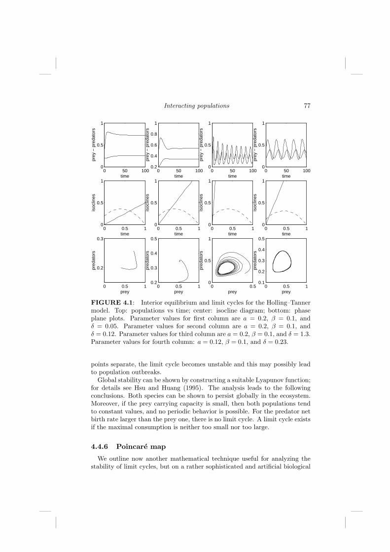
Interacting populations 77
0 50 1000
0.5
1
prey
− p
reda
tors
time
0 0.5 10
0.5
1
isoc
lines
time
0 0.5 1
0.2
0.3
pred
ator
s
prey
0 50 1000.2
0.4
0.6
0.8
1
prey
− p
reda
tors
time
0 0.5 10
0.5
1
isoc
lines
time
0 0.5 10.2
0.3
0.4
0.5
pred
ator
s
prey
0 50 1000
0.5
1
prey
− p
reda
tors
time
0 0.5 10
0.5
1
isoc
lines
time
0 0.50
0.5
1
pred
ator
s
prey
0 50 1000
0.5
1
prey
− p
reda
tors
time
0 0.5 10
0.5
1
isoc
lines
time
0 0.5 10.1
0.2
0.3
0.4
0.5
pred
ator
s
prey
FIGURE 4.1: Interior equilibrium and limit cycles for the Holling–Tannermodel. Top: populations vs time; center: isocline diagram; bottom: phaseplane plots. Parameter values for first column are a = 0.2, β = 0.1, andδ = 0.05. Parameter values for second column are a = 0.2, β = 0.1, andδ = 0.12. Parameter values for third column are a = 0.2, β = 0.1, and δ = 1.3.Parameter values for fourth column: a = 0.12, β = 0.1, and δ = 0.23.
points separate, the limit cycle becomes unstable and this may possibly leadto population outbreaks.
Global stability can be shown by constructing a suitable Lyapunov function;for details see Hsu and Huang (1995). The analysis leads to the followingconclusions. Both species can be shown to persist globally in the ecosystem.Moreover, if the prey carrying capacity is small, then both populations tendto constant values, and no periodic behavior is possible. For the predator netbirth rate larger than the prey one, there is no limit cycle. A limit cycle existsif the maximal consumption is neither too small nor too large.
4.4.6 Poincare map
We outline now another mathematical technique useful for analyzing thestability of limit cycles, but on a rather sophisticated and artificial biological

78 Spatiotemporal patterns in ecology and epidemiology
example. Essentially we consider a prey–predator model that includes theAllee effect and migration.
With the usual notation let us consider the model
dU
dT= A + BU + CU2 − U3 + f(U, V ), (4.56)
dV
dT= H + KV + LV 2 − V 3 + g(U, V ),
where the interaction terms are assumed to be
f(U, V ) = −V [1 + (U − U∗)(V − 2V∗)], (4.57)g(U, V ) = U [1 + (V − V∗)(U − 2U∗)]
(a generalized populations dependence on the predation rate and the conver-sion factor), and the coefficients are chosen in the following particular way:
A = V∗ − U∗ + U3∗ + U∗V 2
∗ , B = 1− 3U2∗ − V 2
∗ , (4.58)
C = 3U∗(> 0), H = U2∗V∗ + V 3
∗ − U∗ + V∗,
K = −1− U2∗ − 3V 2
∗ , L = 3V∗(> 0).
One of course can ask what the quantities U∗ and V∗ are, and here is thesecond artificial aspect of the model. They are supposed to represent anequilibrium value for the two populations. Substituting (4.58)–(4.57) into(4.56) and expanding we find
dU
dT= −(V − V∗) + (U − U∗)− (U − U∗)3 − (U − U∗)(V − V∗)2, (4.59)
dV
dT= U − U∗ + V∗ − V − (U − U∗)2(V − V∗)− (V − V∗)3.
We now introduce x = U −U∗ and y = V −V∗ as perturbations around theequilibrium value, so that (4.59) turns to
dx
dT= −y + x− x3 − xy2 = −y + x(1− x2 − y2), (4.60)
dy
dT= x + y − x2y − y3 = x + y(1− x2 − y2).
At this point, the introduction of polar coordinates becomes natural. Ondifferentiating r2 = x2 + y2 and θ = arctan(y/x), we find
dr
dT=
x
r
dx
dT+
y
r
dy
dT,
dθ
dT=
x
x2 + y2
dy
dT− y
x2 + y2
dx
dT=
x
r2
dy
dT− y
r2
dx
dT.
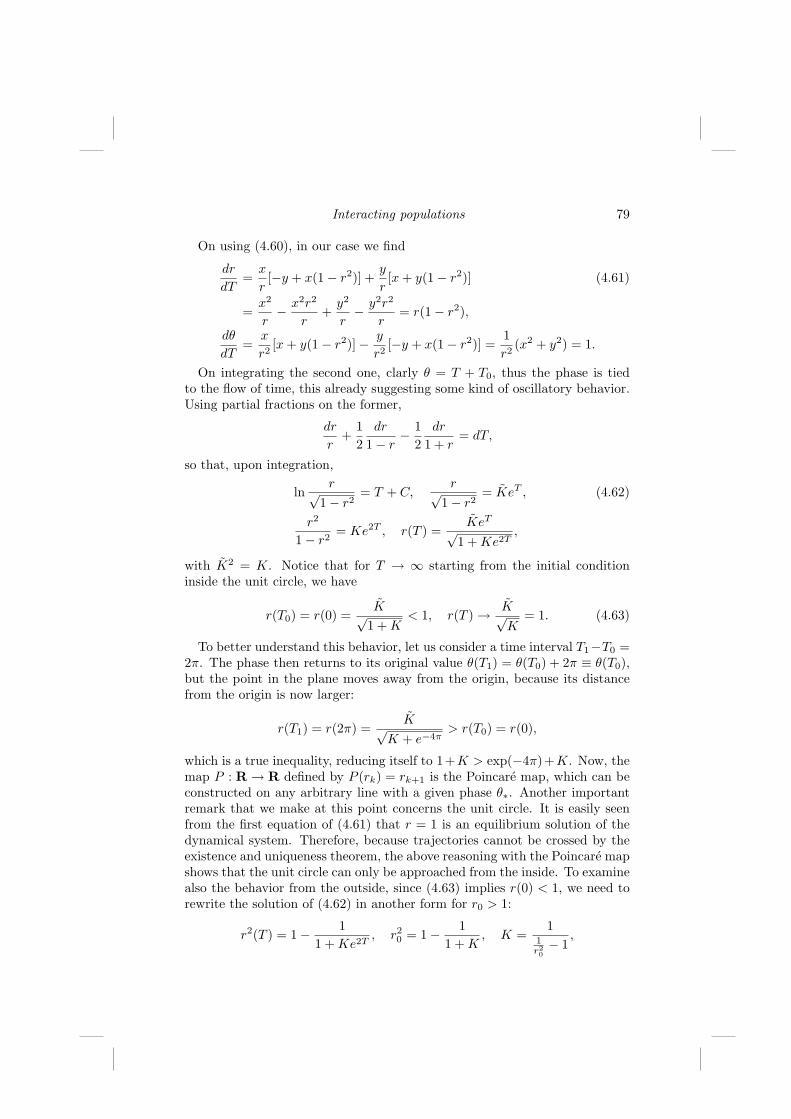
Interacting populations 79
On using (4.60), in our case we find
dr
dT=
x
r[−y + x(1− r2)] +
y
r[x + y(1− r2)] (4.61)
=x2
r− x2r2
r+
y2
r− y2r2
r= r(1− r2),
dθ
dT=
x
r2[x + y(1− r2)]− y
r2[−y + x(1− r2)] =
1r2
(x2 + y2) = 1.
On integrating the second one, clarly θ = T + T0, thus the phase is tiedto the flow of time, this already suggesting some kind of oscillatory behavior.Using partial fractions on the former,
dr
r+
12
dr
1− r− 1
2dr
1 + r= dT,
so that, upon integration,
lnr√
1− r2= T + C,
r√1− r2
= KeT , (4.62)
r2
1− r2= Ke2T , r(T ) =
KeT
√1 + Ke2T
,
with K2 = K. Notice that for T → ∞ starting from the initial conditioninside the unit circle, we have
r(T0) = r(0) =K√
1 + K< 1, r(T ) → K√
K= 1. (4.63)
To better understand this behavior, let us consider a time interval T1−T0 =2π. The phase then returns to its original value θ(T1) = θ(T0) + 2π ≡ θ(T0),but the point in the plane moves away from the origin, because its distancefrom the origin is now larger:
r(T1) = r(2π) =K√
K + e−4π> r(T0) = r(0),
which is a true inequality, reducing itself to 1+K > exp(−4π)+K. Now, themap P : R → R defined by P (rk) = rk+1 is the Poincare map, which can beconstructed on any arbitrary line with a given phase θ∗. Another importantremark that we make at this point concerns the unit circle. It is easily seenfrom the first equation of (4.61) that r = 1 is an equilibrium solution of thedynamical system. Therefore, because trajectories cannot be crossed by theexistence and uniqueness theorem, the above reasoning with the Poincare mapshows that the unit circle can only be approached from the inside. To examinealso the behavior from the outside, since (4.63) implies r(0) < 1, we need torewrite the solution of (4.62) in another form for r0 > 1:
r2(T ) = 1− 11 + Ke2T
, r20 = 1− 1
1 + K, K =
11r20− 1
,

80 Spatiotemporal patterns in ecology and epidemiology
so that, finally,
r2(T ) =Ke2T
1 + Ke2T=
1
1 + e−2T(
1r20− 1
) , (4.64)
r(T ) =[1 + e−2T
(1r20
− 1)]− 1
2
.
Now it is easily seen that the Poincare map satisfies P (r0) > 1, and alsor1 = P (r0) < r0. Indeed, the two conditions respectively become
r1 =[1 + e−4π
(1r20
− 1)]− 1
2
> 1−12 ≡ 1;
[1 + e−4π
(1r20
− 1)]−1
< r20 ,
1 + e−4π
(1r20
− 1)
> r−20 , (1− e−4π)
(1− 1
r20
)> 0,
which are always verified. One final consideration. While the above com-putations have been carried out in almost every detail to double check theassertions, a simple consideration could have led to the same conclusions. In-deed, observe that the system rotates in view of the second equation of (4.61),while the right-hand side of the first one is a cubic polynomial p3(r) with anegative biologically infeasible root r = −1, the second one located in theorigin and the positive one giving the unit circle as already remarked above,r = 1. On plotting it, we find that p3(r) > 0 for 0 < r < 1, so that the originmust be an unstable equilibrium, while r = 1 in polar coordinates is a stablepoint. But that means, in cartesian coordinates, that the unit circle is stable.Thus we have found a stable limit cycle.
As a final biological interpretation of this result, the equilibrium (U∗, V∗)of the original system is unstable and around it there is a stable limit cycle(U∗ − U)2 + (V∗ − V )2 = 1. In these considerations note that the feasibilityof both has not been analyzed, but just assumed.
4.5 Food web
Natural environments are not confined to contain only two populations,rather in general many species intermingle. Their interactions may be of allthe kinds previously discussed, i.e., of competitive nature, or mutually benefi-cial. It turns out that in some circumstances a population that is a predator ofanother one is itself the prey of a higher trophic level predator. In this sectionwe describe a very general model that attempts a more complex description ofreality. It is meant as a brief introduction to food chains. We address a closedecosystem, in which trophic levels from a top predator down to the mineral

Interacting populations 81
nutrients on which the plants feed are accounted for. The analysis shouldassess its possible sustainable equilibria and their stability. The mineral sub-strate and homogeneously mixed populations on three trophic levels are thepopulations in the environment, representing vegetation, herbivore, and car-nivore animals. The homogeneous mixing mathematically implies that thepredation terms are taken to be bilinear, i.e., proportional to both interactingpopulations. This also holds for the interactions among plants and minerals,as the growth of plants depends with direct proportionality on the abundanceof the mineral substrate, while the latter is depleted in a way directly propor-tional to the plants population. It is important to also model the mineral levelin a closed system, as it represents the bottom level to which organic matteris recycled. Questions of time scales are disregarded in this presentation.
Let M represent the minerals, P the plants, H the herbivores, and C thecarnivores. Keeping on following the general convention of the book that allthe parameters are nonnegative unless otherwise stated, the model then isgiven by
dM
dT= m1P + m2H + m3C − b1PM, (4.65)
dP
dT= b2PM −m1P − c1PH,
dH
dT= c2PH −m2H − d1CH,
dC
dT= d2CH −m3C.
From the bottom, i.e., the first equation, decaying organic matter is con-verted into minerals and they in turn are depleted by the plants’ uptake atrate b1 for their own growth. The second equation describes this uptake fromthe plants’ viewpoint, at rate b2 < b1. Plants are also grazed by herbivoresat rate c1 and have an intrinsic mortality m1. Similar considerations holdfor the herbivores, feeding at rate c2 on plants, and for carnivores feeding onthe former at rate d2. Notice that we do not assume logistic growth, in partto keep the mathematics tractable, in view of the nine parameters the modelalready contains, as well as to investigate the system’s behavior assuming itto be closed, i.e., when the possible carrying capacities are dictated by theavailability of the nutrients at the lower trophic level. Indeed, as the onlyfood source is given by the trophic level just below the one considered, aslong as the latter supports the former, the assumption of “unlimited” growthis sound.
To reduce the parameters, let us introduce new dependent variables asfollows: M = αx1(t), P = βx2(t), H = γx3(t), C = δx4(t), T = πt, and
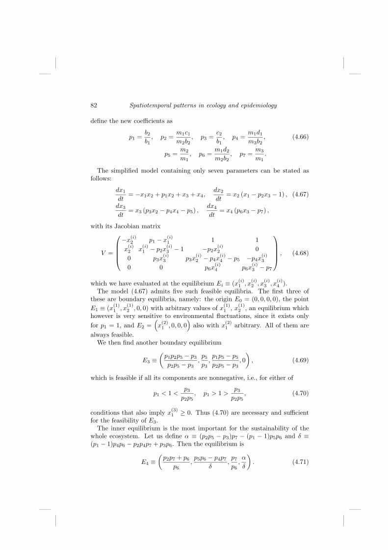
82 Spatiotemporal patterns in ecology and epidemiology
define the new coefficients as
p1 =b2
b1, p2 =
m1c1
m2b2, p3 =
c2
b1, p4 =
m1d1
m3b2, (4.66)
p5 =m2
m1, p6 =
m1d2
m2b2, p7 =
m3
m1.
The simplified model containing only seven parameters can be stated asfollows:
dx1
dt= −x1x2 + p1x2 + x3 + x4,
dx2
dt= x2 (x1 − p2x3 − 1) , (4.67)
dx3
dt= x3 (p3x2 − p4x4 − p5) ,
dx4
dt= x4 (p6x3 − p7) ,
with its Jacobian matrix
V =
−x(i)2 p1 − x
(i)1 1 1
x(i)2 x
(i)1 − p2x
(i)3 − 1 −p2x
(i)2 0
0 p3x(i)3 p3x
(i)2 − p4x
(i)4 − p5 −p4x
(i)3
0 0 p6x(i)4 p6x
(i)3 − p7
, (4.68)
which we have evaluated at the equilibrium Ei ≡ (x(i)1 , x
(i)2 , x
(i)3 , x
(i)4 ).
The model (4.67) admits five such feasible equilibria. The first three ofthese are boundary equilibria, namely: the origin E0 = (0, 0, 0, 0), the pointE1 ≡ (x(1)
1 , x(1)2 , 0, 0) with arbitrary values of x
(1)1 , x
(1)2 , an equilibrium which
however is very sensitive to environmental fluctuations, since it exists onlyfor p1 = 1, and E2 =
(x
(2)1 , 0, 0, 0
)also with x
(2)1 arbitrary. All of them are
always feasible.We then find another boundary equilibrium
E3 ≡(
p1p2p5 − p3
p2p5 − p3,p5
p3,p1p5 − p5
p2p5 − p3, 0
), (4.69)
which is feasible if all its components are nonnegative, i.e., for either of
p1 < 1 <p3
p2p5, p1 > 1 >
p3
p2p5, (4.70)
conditions that also imply x(3)1 ≥ 0. Thus (4.70) are necessary and sufficient
for the feasibility of E3.The inner equilibrium is the most important for the sustainability of the
whole ecosystem. Let us define α ≡ (p2p5 − p3)p7 − (p1 − 1)p5p6 and δ ≡(p1 − 1)p4p6 − p2p4p7 + p3p6. Then the equilibrium is
E4 ≡(
p2p7 + p6
p6,p5p6 − p4p7
δ,p7
p6,α
δ
). (4.71)

Interacting populations 83
The feasibility conditions for E4 require that x(4)2 ≥ 0, x
(4)4 ≥ 0, as the
remaining components are obviously nonnegative. These conditions reduce toeither
α ≥ 0, δ ≥ 0, p5p6 ≥ p4p7 (4.72)
orα ≤ 0, δ ≤ 0, p5p6 ≤ p4p7. (4.73)
Model properties
To establish the behavior of the system near each equilibrium point, weneed to determine the signs of the eigenvalues of the Jacobian (4.68).
The first equilibrium E0 has one zero eigenvalue λ1 = 0, and the otherones negative, λ2 = −1, λ3 = −p5 and λ4 = −p7. The origin is thus astable equilibrium, neutral along the x1-axis. Also, for E2 there is a vanishingeigenvalue, λ1 = 0, the other ones being λ2 = x
(2)1 − 1, λ3 = −p5, and λ4 =
−p7. Thus, if x(2)1 ≤ 1, the equilibrium is stable, else it is unstable.
The first eigenvalue of E3 is p6x(3)3 − p7. The signs of the other ones can
be obtained from the Routh–Hurwitz conditions applied to the characteristicequation. They give x
(3)2 x
(3)3 (p2p3x
(3)2 + 1) > 0, which is obviously true, and
p3x(3)2 x
(3)3 (p2x
(3)2 − 1) > 0. Thus E3 is stable if and only if the first eigenvalue
is negative, i.e., p6x(3)3 < p7 and the further condition p2p5 > p3 is satisfied,
which falsifies the first equation in (4.70). Hence feasibility must be given bythe second condition (4.70), which yields p1 > 1.
Let N(λ) ≡ x(4)2 [λ2(p1 − x
(4)1 ) + λp3x
(4)3 + p3p6x
(4)3 x
(4)4 (1 + p1 − x
(4)1 )] and
D(λ) ≡ x(4)2 + λ. The root-finding problem for the characteristic equation at
E4 can be restated as the intersection of the two curves
K(λ) = λ3 + λ(p4p6x(4)3 x
(4)4 + p2p3x
(4)2 x
(4)3 ), R(λ) ≡ N(λ)
D(λ).
Now K has only a real root at the origin and K ′(λ) > 0 for every λ, so thatK(λ) ∼ λ3 as λ →∞. Instead, R(λ) ∼ x
(4)2 (p1− x
(4)1 )λ + p3x
(4)2 x
(4)3 , and also
as λ → ∞. The function R(λ) has a vertical asymptote located at the zero−x
(4)2 of D(λ), and two zeros at the roots of N(λ):
λ± ≡−p3x
(4)3 ±
√p23(x
(4)3 )2 − 4(p1 − x
(4)1 )p3p6x
(4)3 x
(4)4 (1 + p1 − x
(4)1 )
2(p1 − x(4)1 )
.
Now it is easy to verify that λ± < 0 if p1 > x(4)1 and 1 + p1 − x
(4)1 > 0.
On the other hand, for p1 < x(4)1 and 1 + p1 − x
(4)1 > 0, λ+ < 0 < λ−.
Finally, for p1 < x(4)1 and 1 + p1 − x
(4)1 < 0, λ± > 0. Also, notice that
R(0) = 1 + p1 − x(4)1 ≡ p1 − p2x
(4)3 .

84 Spatiotemporal patterns in ecology and epidemiology
From this analysis, there is always an intersection between K and R,K(λ∗) = R(λ∗) occurring for λ∗ > 0, unless p1 < x
(4)1 and 1 + p1 − x
(4)1 < 0.
We have thus determined easily verifiable sufficient instability conditions forE4. The necessary and sufficient conditions for stability are instead given bythe following three Routh–Hurwitz conditions:
p6(p3 + p1p4) < p4(p2p7 + 1), x(4)2 [p2p7 + p6(1− p1)] > p3p7, (4.74)
p6x(4)4 (x(4)
2 − p4x(4)3 ) + (1− p2)[p3x
(4)3 + x
(4)2 (p1 − x
(4)1 )] > 0.
Observe further that letting
A = x(4)2 > 0, B = p1 − x
(4)1 = p1 − p2x
(4)3 − 1,
D = x(4)3 , F =
1p4
[p6p3x(4)2 − p5p6],
the characteristic equation can be written as
ϕ(λ) =4∑
i=0
aiλi, a4 = 1, m3 = x
(4)2 , m2 = −AB + p2p3AD + p4DF,
m1 = −p3AD + p2p3A2D + p4ADF, a0 = −ADF (p3 + p4B).
Since ϕ is a quartic, ϕ(λ) → +∞ as λ → ±∞. Its inflection pointsϕ′′(λ±) = 0 are real if ∆ ≡ 9m2
3 − 24a4 > 0, in which case it is easily seenthat they lie in the negative left half-plane, as their abscissae are
λ± =112
[−3m3 ±√
∆] ≤ 0. (4.75)
In such a case,a0 = ϕ(0) > 0, m1 = ϕ′(0) > 0 (4.76)
are sufficient conditions for stability, ensuring that no positive eigenvalue ex-ists. For ∆ < 0 instead, no inflection point exists, but again satisfying both(4.76) ensures once more the stability of E4.
Results and discussion
The equilibrium E4 can also be investigated numerically, to find featuresthat are analytically harder to show. Indeed for the parameters, p1 = 1.84(Figure 4.2) and p1 = 1.89 (Figure 4.3), p2 = 0.6, p3 = 0.4, p4 = 4.25,p5 = 0.9, p6 = 0.555, p7 = 0.9 exhibit limit cycles. We then numerically tryto modify the parameters one at a time to investigate the effects of this change.Changes toward smaller values of p1 are generally reflected in oscillations ofsmaller amplitude around a smaller reference value. The value p1 = 0.5brings a collapse of the limit cycle first toward the corresponding underlyingequilibrium value E4, then a further decrease of p1 leads to the equilibrium

Interacting populations 85
290 292 294 296 298 3000
5
10
15
20
25
30
35
40
time
Foodweb Model
mineralsplantsherbivorescarnivores
290 292 294 296 298 30010
0
101
102
time
p1=1.84, p2=0.6, p3=0.4, p4=4.25, p5=0.9, p6=0.555, p7=0.9
mineralsplantsherbivorescarnivores
FIGURE 4.2: Persistent oscillations around the inner equilibrium E4
shown in standard and semilogarithmic plots.
E3 where only one population is wiped out, and then finally induces a furtherchange also of this other equilibrium to the equilibrium E2.
Changes toward higher values of p2 damp out the oscillations so as to getback to E4. Smaller values instead lead one of the species to grow towardvery high values while still oscillating. Increasing p7 instead gives us againthe stable equilibrium E3.
Decreasing p3 from the reference value produces limit cycles, again aroundlower values of the equilibrium, and the smaller the value of p3, the lower theequilibrium is. Increasing it instead to p3 = 1, the oscillations disappear andat least two trophic levels prevail.
The parameters p4 and p5 finally affect much less the model behavior, al-though a bifurcation value at p5 = 8.33122 exists, this time from the referencevalues p1 = 1.86, p2 = 0.6, p3 = 0.415, p4 = 4.25, p5 = 0.555, p6 = 0.9. Alsofrom these latter values a bifurcation value p6 = 0.807 is found driving thesystem back to E3.
In summary, the results obtained are meaningful. Indeed, the neutral sta-bility of the origin is easily explained since an empty closed system “by def-inition” remains empty as long as migrations into it are not allowed. At E2
the ecosystem is lifeless and stable at an arbitrary level x(2)1 . This is possible,
however, only if the amount of the matter is below a threshold level. Thus thenutrients need to be at a minimum level, to avoid collapse of the plants andeventually of the ecosystem as a whole. An equilibrium environment is shownto exist, in which plants and herbivores can coexist in absence of carnivores,by the range of parameters leading to a stable E3, namely, if p1 > 1.

86 Spatiotemporal patterns in ecology and epidemiology
296 297 298 299 3000
100
200
300
400
500
600
700
800
time
Foodweb Model
mineralsplantsherbivorescarnivores
296 297 298 299 30010
0
101
102
103
time
p1=1.89, p2=0.6, p3=0.4, p4=4.25, p5=0.9, p6=0.555, p7=0.9
mineralsplantsherbivorescarnivores
FIGURE 4.3: Change in the oscillations around the inner equilibrium E4
due to a change in p1, the cycles become wider, around a higher referencevalue; note that the vertical scale differs from the one in Figure 4.2.
The point where the whole ecosystem thrives is E4. We have found con-ditions on its parameters ensuring feasibility, (4.72) or (4.73), necessary andsufficient stability conditions (4.74), and easier to verify sufficient conditions(4.76). However, the numerical simulations show that when E4 is unstable,the model first exhibits sustained oscillations around this equilibrium andthen trajectories may collapse into one of the former equilibria. When thedynamics is forced toward boundary equilibria, some of the populations dis-appear; in biological terms, we have loss of biodiversity. The ultimate failureof the system is thus represented by E1, i.e., disappearance of life in someor all of its forms. This may very well be provoked by tampering with themodel parameters by external factors, which may be due to “natural” causes,as wheather, sunlight, and so on, or man-made.
Although this study is far too elementary to draw any serious forecastson the global environment, it nevertheless shows that sustained oscillations inthe ecosystem are feasible and compatible with human activities, provided thelatter do not induce too drastic changes in the parameters. A simple modellike the one presented here thus shows that it is very important to assess ourpresent stand, to understand whether the changes nowadays occurring on aworldwide scale are going to be permanent or are only part of a temporaryand thus still reversible process.

Interacting populations 87
4.6 More about chaos
In the previous sections, we have been dealing mostly with either a system’srelaxation to a stable steady state or with periodic solutions due to a stablelimit cycle. In a time-continuous population community with the number ofspecies more than two, however, there can be a more complicated and moreexotic type of dynamics which is known as (deterministic) chaos.
As an instructive example, following the work by Hastings and Powell(1991), let us consider a simple food web (or, rather, a food chain) thatincludes three trophic levels, i.e., a prey, its predator, and a top predator:
du
dt= u(1− u)− a1uv
1 + b1u, (4.77)
dv
dt=
a1uv
1 + b1u− a2vw
1 + b2v− d1v ,
dw
dt=
a2vw
1 + b2v− d2w
(in dimensionless variables), where u, v, and w are the densities of prey, preda-tor, and top predator, respectively, and a1,2, b1,2 and d1,2 are parameters.
The system (4.77) is difficult to study analytically, but it is more or lessstraightforward to reveal its main properties by means of numerical simu-lations. A problem arising on this way is that it depends on as many assix parameters. Therefore, a comprehensive study would require thousandsof simulation runs accomplished for different parameter sets. Alternatively,however, since our goal here is to give an example of chaotic dynamics ratherthan to fulfil a detailed study of the system properties, we can fix most of theparameters at a certain hypothetical value and study the system’s behavioras a response to variations in the remaining “controlling parameter.”
It is well-known (e.g., see Murdoch and Oaten, 1975, and also Section 10.1of Chapter 10) that stability of a prey–predator system with Holling typeII response of predator essentially depends on the half-saturation constant,and hence on parameter b1. We can thus assume that b1 is likely to controlthe properties of the tritrophic system (4.77) as well and choose it as thecontrolling parameter.
Numerical simulations show that for small values of b1 the system normallypossesses a stable steady state. With an increase in b1, its stability is even-tually broken through the Hopf bifurcation and a stable limit cycle appears;see the left-hand panel of Figure 4.4. With a further increase in b1, the sys-tem undergoes a series of period-doubling bifurcations and the shape of thelimit cycle becomes more and more complicated (cf. Figure 4.4b) until it turnsinto a strangely looking attractor that no longer bears any resemblance to alimit cycle; see Figure 4.5. Correspondingly, the oscillations of the populationdensities versus time become irregular, too.

88 Spatiotemporal patterns in ecology and epidemiology
0.6
0.8
1
0
0.2
0.4
0.6
10
11
12
13
uv
w
a) A simple limit cycle for b1 = 2.2.
0.4
0.6
0.8
1
0
0.2
0.4
0.6
8
9
10
11
12
uv
w
b) A multiple cycle for b1 = 2.6.
FIGURE 4.4: Dynamics of system (4.77); see details in the text. Parame-ters are a1 = 5.0, a2 = 0.1, b2 = 2.0, d1 = 0.4, and d2 = 0.0086.
A visually different shape of attractor, however, is surely not enough toconclude that the system dynamics has acquired any qualitatively new fea-tures. Indeed, theoretically speaking, the attractor shown in Figure 4.5 couldstill be a multiple cycle. What actually distinguishes chaos from a multiperi-odic dynamics, however complicated the latter may be, is a different responseto variations of the initial conditions. While a (multi)periodic limit cycleis stable with regards to such variations, a fundamental property of chaoticdynamics is a special type of sensitivity so that distance d between any twoinitially closed trajectories grows with time exponentially. This property isusually quantified by the dominant Lyapunov exponent:
λD = limd(0)→0, t→∞
1t
log[
d(t)d(0)
](4.78)
(cf. Nayfeh and Balachandran, 1995).It is very difficult to prove chaotic behavior analytically, but it is relatively
easy to demonstrate it numerically. Figure 4.6 shows the density of the toppredator versus time calculated for two very close sets of initial conditions;u1(0) = u2(0), v1(0) = v2(0) and w1(0) − w2(0) = 0.001. It is readily seenthat, while at an earlier stage of the system dynamics the trajectories remainclose, the discrepancy between the solutions grows steadily so that for t '2000 it becomes on the same order as that of the solutions themselves. Thecorresponding value of λD can then be roughly estimated as 0.01.
Runaways of system trajectories due to the system’s sensitivity to the initialconditions make intermediate-term prediction of the system state impossible,and that may have profound implications. This is one of the reasons why theissue of chaos – in particular, in population dynamics and ecology – has beenattracting a lot of attention over the last three decades; e.g., see May (1974),

Interacting populations 89
0.20.4
0.60.8
1
0
0.2
0.4
0.6
8
9
10
11
12
uv
w
FIGURE 4.5: Chaotic dynamics of system (4.77) observed for b1 = 2.7;other parameters are the same as in Figure 4.4. The shown trajectory iscalculated for 5000 ≤ t ≤ 10000; the trajectory for 0 < t < 5000 was omittedin order to exclude the impact of transients.
Berryman and Millstein (1989), Scheffer (1991b), Hastings et al. (1993), andCushing et al. (2003).
Another example of a population dynamics model exhibiting chaos is givenby a Lotka–Volterra-type system with one predator and two preys (cf. Gilpin,1979; Arneodo et al., 1980):
du1
dt= (1− r11u1 − r12u2 − r13v)u1 , (4.79)
du2
dt= (1− r21u1 − r22u2 − r23v)u2 ,
dv
dt= (−1 + r31u1 + r32u2 − r33v) v ,
where u1, u2 and v are the (dimensionless) densities of prey 1, prey 2, andpredator, respectively, and all coefficients rij are assumed to be nonnegative.Having chosen the predation rate r31 as a controlling parameter and otherparameters fixed at some hypothetical values, Schaffer and Kot (1986) showedthat the system (4.79) exhibits onset of chaos through the period-doublingbifurcation scenario when r31 increases to a certain critical value.
A further discussion of prerequisites and implications of chaos in “multi-

90 Spatiotemporal patterns in ecology and epidemiology
0 500 1000 1500 2000
8
9
10
11
12
Time
Pop
ulat
ion
Den
sity
FIGURE 4.6: (See color insert.) Top predator density vs time: there is agrowing discrepancy between two initially close trajectories (w1(0)−w2(0) =0.001) in the chaotic regime of system (4.77). Parameters are the same as inFigure 4.5.
species systems”1 can be found in Rinaldi and Feo (1999).Note that, when looking for chaotic dynamics in a time-continuous model
described by a system of ordinary differential equations, the condition thatthe number of interacting species must not be less than three is essential.Indeed, the solution uniqueness theorem, which is valid in a general case ofn species system (2.1) under some unrestrictive and biologically reasonableassumptions about the properties of the interaction terms Fi, obviously rulesout a possibility of trajectories intersection. In the case of two-species system,where the phase space is reduced to a plane, it thus excludes existence of anattractor more complicated than a limit cycle. The situation is thus verymuch different from time-discrete systems where chaos can occur even in asingle species model; see Section 3.4.
It should be mentioned here that, although there are many theoretical ar-guments showing that chaos should be a common phenomenon in populationdynamics (and chaos has indeed been observed for at least two different lab-oratory populations; see Costantino et al., 1997; Becks et al., 2005), a con-clusive evidence of chaos in ecological data is still lacking. This disagreementbetween theory and available data has been a subject of continuing intensivediscussion and controversy; the two reasons that are usually mentioned as a
1In this context, systems with the number of species greater than two.
Interacting populations 91
probable explanation why chaos is not immediately seen in ecological dynam-ics are the impact of noise and an insufficient length of ecological time series.The latter also raises a more fundamental concern that chaos in ecosystemsdynamics cannot be seen at all (even if it may be an intrinsic property of agiven system) because of the impact of transients (Hastings, 2001, 2004). Asa whole, however, the question of whether mother nature is chaotic and if not,why not (cf. Berryman and Millstein, 1989; Hastings et al., 1993) yet remainslargely open.
4.7 Age-dependent populations
This is probably the most theoretical section of the whole book. We startby illustrating a simple example in some of its fine details to describe theanalytical technique used. The purpose of the later sections is to presentthe well-known contraction mapping principle on a nontrivial, rather sophis-ticated application. We have already encountered fixed points in the earlierchapter on a single discrete population. In this one the continuous case is dis-cussed, allowing interactions among two populations. Excellent and thoroughreferences on this topic for the interested reader are the books by Cushing(1998), Iannelli (1995), and Webb (1985).
Lotka (1956) and von Foerster (1959) in population theory and McKendrick(1926) in the context of epidemics introduced an age-dependent descriptionof the population in which instead of the total population size as a function oftime, they considered as the dependent variable a density function, which givesat every instant the number of individuals in the same age group, technicallycalled a cohort, and looks at its evolution in time. The model is formulatedas a hyperbolic partial differential equation of the first order.
Leslie (1945; 1948) considered a discrete system, in which each componentof a vector describes the cohort in a certain age interval, while the evolutionof the population is described by a matrix, the Leslie matrix, whose entriescontain the mortality of each cohort.
We will consider only the continuous-time version, and describe now howto obtain the governing equations.
If u (a, T ) represents the density of the population, the total population is inthis case provided by summing the density over all possible ages. Technically,two possibilities arise, namely, to assume that there is a maximum allowedage A, so that u (a, T ) ≡ 0 for all a ≥ A at all times T , or simply to allow allpossible ages up to ∞, in which case mathematically we need to assume thematernity to have compact support, so as to be able to meaninfully define theintegral that follows. This second possibility will be used later in Section 6.3.

92 Spatiotemporal patterns in ecology and epidemiology
Thus
U(T ) =∫ A
0
u (a, T ) da. (4.80)
The above equation represents then the relationship of this model with theprevious ones, which are independent of age.
If we now let a time δT go by, we find that all individuals will be aged a+δT ,apart from those who in the meantime passed away. This remark shows thatthe differentials of age and time are the same, dT ≡ da, or, integrating,a = T −T0, where T0 denotes the “birhdate” of the cohort. Thus, introducingthe individual mortality rate m(a, T ), we find the balance equation:
u (a + δT, T + δT )− u (a, T )δT
≡ u (a + δT, T + δT )− u (a + δT, T )δT
+u (a + δT, T )− u (a, T )
δT= m(a, T )u (a, T ) . (4.81)
In general, the mortality function is independent of time, or better, it de-pends on time implicitly via the density u (a, T ) itself, or rather said, throughthe population m ≡ m (a, U(T )). As a first approach, however, for the nextconsiderations, let us take it to be only age dependent, namely, m ≡ m (a).Letting δT → 0, we find the basic equation governing the age-dependentpopulation models:
∂u (a, T )∂T
+∂u (a, T )
∂a+ m(a)u (a, T ) = 0. (4.82)
The model is still incomplete, as an initial condition is needed, which in thiscase is provided by an initial density u (a, 0) = φ(a), but above all becausewe need to describe the process by which new individuals are added to thepopulation. To this end, let us introduce the maternity function β(a, T ) ≡β(a, U (T )), again implicitly a function of time via the population size. Itrepresents the reproduction of the cohort in the population aged a at time T .Now the newborns can be calculated by summing the contributions of eachindividual reproduction function over all possible ages. The newborns B(T )at time T are thus given by
B(T ) =∫ A
0
β(a, U (T ))u (a, T ) da. (4.83)
The model thus formulated is an initial and boundary value problem, inthe sense that the “boundary” is expressed by the fact that age can never benegative, and the new individuals coming into the population are the newbornsof age 0; they are accounted for by the boundary term (4.83).
The characteristics of (4.82) are straight lines, as dT = da, which in para-metric form are written T = s + T0, a = s. Notice that the tangent unit

Interacting populations 93
vector to these lines is t = 1√2(1, 1)T . Remembering the meanings of age and
time differentials, observe that
ds2 = dT 2 + da2, ds =√
2da. (4.84)
Consider u(s) ≡ u(s, s + T0), i.e., the density along the characteristics. Ingeneral, the partial differential operator on the left of (4.82) represents thederivative of the restriction of the function u to the caracterists,
Du(s, T ) ≡ limδa→0
u (s + δa, T + δa)− u (s, T )δa
=du(s)
ds. (4.85)
Notice on the other hand that the partial differential operator on the left-hand side of (4.82) is related to the directional derivative of u along thecharacteristics Dtu. Indeed, since
Du =∂u
∂T+
∂u
∂a= ∇u · (1, 1)T =
√2∇u · t ≡
√2Dtu. (4.86)
Equations (4.86) and (4.85) are related, representing the same concept, thedifference being the use of the arclength.
To better motivate the use of the latter, let us ignore dependence on timein the mortality function, which is then only dependent on age. Thus u(a, T )will be subject to m(a), and u(a + δa, T + δT ) will be subject to m(a +δT ) = m(a + δa). But letting δT go by, from u(a0, t0) = u(s0) measuredalong one of the characteristics, subject to the mortality m(a0) we arriveat u(a0 + δa, T0 + δT ) = u(s0 + δs). Recalling (4.84), the density at thepoint (a0 + δa, T0 + δT ) would be subject to the mortality m(a0 +
√2δa)
rather than to the correct one m(a0 + δa). This consideration tells us thatalong the characteristics we need to use as a parameter the arclength, i.e., thenormalized s via the factor
√2, namely, σ = 1√
2s.
With this position, we can then describe the evolution of the density u asfollows:
[u(s + δs√
2)− u(
s√2)]√
2δs
= −m(s√2)u(
s√2).
Upon taking the limit as δσ → 0,
du
dσ(σ) = m(σ)u(σ),
du
u= m(σ)dσ,
and integration setting s =√
2α then finally gives
ln u(σ)− ln u(0) = −∫ σ
0
m(α)dα, u(σ) = u(0) exp(−
∫ s
0
m(α)dα
).
This is the process known as integration along the characteristics of the firstorder partial differential equation; for a geometric interpretation see Zach-manoglou and Thoe (1976).

94 Spatiotemporal patterns in ecology and epidemiology
We now need to distinguish two cases. When the characteristic meets theinitial times, i.e., T0 > 0, notice that when we start counting time the cohort isalready aged a. In such a case, the value of u(s) is provided by the value of theinitial distribution, ψ(a), so that u(0) = u(a, 0) = ψ(a). For T0 < 0, instead,when T0 denotes the birthtime of the cohort, u(0) = u(0, T0) = B(T0), and thelatter is determined from (4.83). Thus, for a > T and a < T , we respectivelyhave
u(a, T ) = ψ(a− T ) exp
[−
∫ a−T
0
m(α)dα
], (4.87)
u(a, T ) = B(T − a) exp
[−
∫ T−a
0
m(α)dα
]. (4.88)
Upon substitution into the population equation, we respectively find forξ = a− T and η = T − a,
U(T ) =∫ A
T
u(a, T )da +∫ T
0
u(a, T )da
=∫ A−T
0
u(ξ, T )dξ +∫ T
0
u(a, T )da.
The problem is then finally completely described by the pair of integral equa-tions (4.83) and (4.89):
U(T ) =∫ A−T
0
ψ(ξ) exp
(−
∫ ξ
0
m(α)dα
)dξ (4.89)
+∫ T
0
B(η) exp(−
∫ η
0
m(α)dα
)dη.
By instead multiplying by the maternity function (4.87) and using again(4.83), with the very same steps we find
B(T ) =∫ A−T
0
β(ξ, U (T ))u(ξ, T )dξ +∫ T
0
β(a, U (T ))u(a, T )da, (4.90)
which leads to the single integral equation
B(T ) =∫ A−T
0
ψ(ξ)β(ξ, U (T )) exp
(−
∫ ξ
0
m(α)dα
)dξ (4.91)
+∫ T
0
B(η)β(T + η, U (T )) exp(−
∫ η
0
m(α)dα
)dη.
It is also possible to introduce survival probabilities and relate this equationto the renewal equation of probability theory; for details see Cushing (1998).
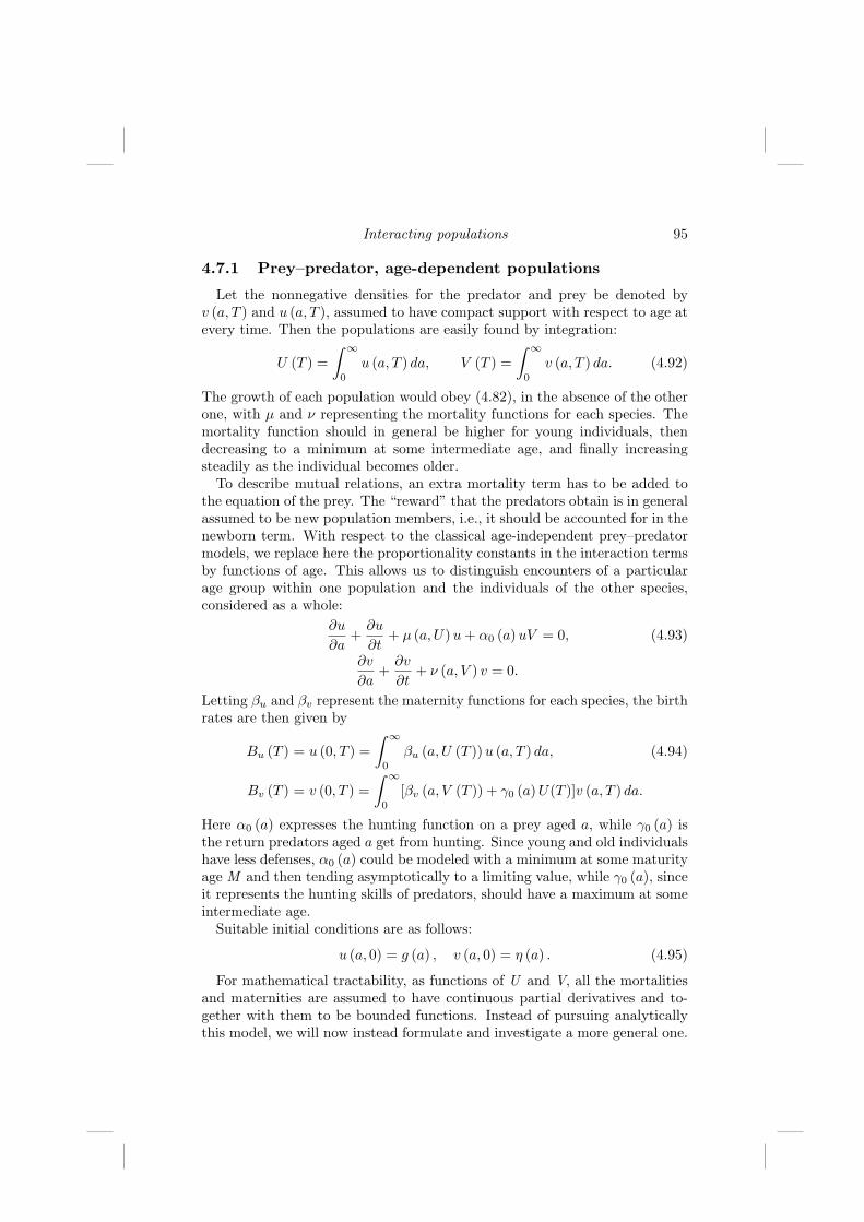
Interacting populations 95
4.7.1 Prey–predator, age-dependent populations
Let the nonnegative densities for the predator and prey be denoted byv (a, T ) and u (a, T ), assumed to have compact support with respect to age atevery time. Then the populations are easily found by integration:
U (T ) =∫ ∞
0
u (a, T ) da, V (T ) =∫ ∞
0
v (a, T ) da. (4.92)
The growth of each population would obey (4.82), in the absence of the otherone, with µ and ν representing the mortality functions for each species. Themortality function should in general be higher for young individuals, thendecreasing to a minimum at some intermediate age, and finally increasingsteadily as the individual becomes older.
To describe mutual relations, an extra mortality term has to be added tothe equation of the prey. The “reward” that the predators obtain is in generalassumed to be new population members, i.e., it should be accounted for in thenewborn term. With respect to the classical age-independent prey–predatormodels, we replace here the proportionality constants in the interaction termsby functions of age. This allows us to distinguish encounters of a particularage group within one population and the individuals of the other species,considered as a whole:
∂u
∂a+
∂u
∂t+ µ (a, U) u + α0 (a)uV = 0, (4.93)
∂v
∂a+
∂v
∂t+ ν (a, V ) v = 0.
Letting βu and βv represent the maternity functions for each species, the birthrates are then given by
Bu (T ) = u (0, T ) =∫ ∞
0
βu (a, U (T )) u (a, T ) da, (4.94)
Bv (T ) = v (0, T ) =∫ ∞
0
[βv (a, V (T )) + γ0 (a) U(T )]v (a, T ) da.
Here α0 (a) expresses the hunting function on a prey aged a, while γ0 (a) isthe return predators aged a get from hunting. Since young and old individualshave less defenses, α0 (a) could be modeled with a minimum at some maturityage M and then tending asymptotically to a limiting value, while γ0 (a), sinceit represents the hunting skills of predators, should have a maximum at someintermediate age.
Suitable initial conditions are as follows:
u (a, 0) = g (a) , v (a, 0) = η (a) . (4.95)
For mathematical tractability, as functions of U and V, all the mortalitiesand maternities are assumed to have continuous partial derivatives and to-gether with them to be bounded functions. Instead of pursuing analyticallythis model, we will now instead formulate and investigate a more general one.
96 Spatiotemporal patterns in ecology and epidemiology
4.7.2 More about age-dependent populations
We extend the model formulated in the previous section by considering anenvironment in which several population are present and interact, accountingfor species that either live in symbiosis or compete for common resources, orsuch that some species are hunted by others. The approach follows closelyGurtin and McCamy (1974), and the results are related to those obtained vianonlinear semigroups in Webb (1985). Here we also allow nonlinear interac-tions, by letting both the maternity and mortality functions for each speciesbe influenced by all the other species. The necessary assumption will of coursebe that these modified mortalities retain positive signs so that they will nevergenerate newborns of some positive age. The modifications increase or de-crease each species density according to the type of interaction with otherspecies. Similar remarks hold for the maternities as well, which are alwayspositive, i.e., never generating a negative number of newborns.
Let xi (a, t), i = 1, ..., N represent the densities of the N populations, as-sumed to be of compact support with respect to age at any given time t. Thisensures that the population sizes are well defined:
Xi (t) =∫ ∞
0
xi (a, t) da. (4.96)
Letting X ≡ (X1, . . . , XN )T , the birth rates can then be defined as
Bi (t) = xi (0, t) =∫ ∞
0
βi (a,X (t)) xi (a, t) da. (4.97)
Here βi represents the maternity function for the ith species. The model thenbecomes
∂xi
∂t+
∂xi
∂a+ µi (a,X (t))xi (a, t) = 0, (4.98)
with initial conditions
xi (a, 0) = φi (a) . (4.99)
The maternity and mortality functions are assumed to be continuous andnonnegative on R+ × (R+)N . Moreover, for every multiindex α, 0 ≤ |α| ≤ Pfor some P, the maternity and mortality are bounded above, as functions ofX ∈ (R+)N , together with their mixed partial derivatives:
∂αβi
∂Xα,∂αµi
∂Xα, i = 1, ..., N.
As functions of age, for the maternity and mortality functions, the consid-erations of the previous section hold. Thus the following quantities are well

Interacting populations 97
defined:
µ0 = sup (µi (a,X) : (a,X) ∈ Ω; i = 1, ..., N) ; (4.100)
µ′ = sup(
∂µi
∂Xj(a,X) : (a,X) ∈ Ω; i, j = 1, ..., N
); (4.101)
β0 = sup (βi (a,X) : (a,X) ∈ Ω; i = 1, ..., N) ; (4.102)
β′ = sup(
∂βi
∂Xj(a,X) : (a,X) ∈ Ω; i, j = 1, ..., N
). (4.103)
Moreover, assume
b∗ = sup βi (a,X) : a ≥ 0, Xj ≥ 0, i, j = 1, ..., N (4.104)m∗ = inf µi (a,X) : a ≥ 0, Xj ≥ 0, i, j = 1, ..., N . (4.105)
Integral reformulation – local existence
For i = 1, ..., N , let xi denote a solution of the problem up to some timeT > 0. Let us then set
xi (h) = xi
(a0 + h, t0 + h
), Xi = Xi
(t0 + h
), µi (h) = µi
(a0 + h, X (h)
).
As it was shown at the beginning of this section, since
dxi (h)dh
=∂xi
∂a+
∂xi
∂t,
the model becomes the following system of ordinary differential equations:
dxi (h)dh
+ µi (h) xi (h) = 0.
Integrating and rephrasing,
xi (h) = xi (0) exp
(−
∫ h
0
µi (s) ds
),
xi
(a0 + h, t0 + h
)= xi
(a0, t0
)exp
(−
∫ h
0
µi (s) ds
).
For a ≥ t, choose a0 = a−t, t0 = 0, h = t, and for a ≤ t, let a0 = 0, t0 = t−a,h = a, to find the densities in terms of the initial and boundary conditions
xi (a, t) = φi (a− t) exp(−
∫ t
0
µi (a− t + s,X (s)) ds
)(4.106)
for a ≥ t, and
xi (a, t) = Bi (t− a) exp(−
∫ a
0
µi (s,X (t− a + s)) ds
)(4.107)
98 Spatiotemporal patterns in ecology and epidemiology
for a ≤ t.Let
Ki (α, t,X) = exp(−
∫ t
t−a
µi (τ + t− α,X (τ)) dτ
),
Li (v, t,X) = exp(−
∫ t
0
µi (v + τ,X (τ)) dτ
).
Integrating (4.106) and (4.107) gives the total population sizes and repeatingthe operation on the same formulas multiplied by the maternities provides thetotal birth rates. Mathematically, then,
Xi (t) =∫ t
0
Bi (u) Ki (t− u, t,X) du (4.108)
+∫ ∞
0
φi (v)Li (v, t,X) dv,
Bi (t) =∫ t
0
Bi (u) βi (t− u,X)Ki (t− u, t,X) du (4.109)
+∫ ∞
0
φi (v)βi (t + v,X)Li (v, t,X) dv.
Thus our model is reduced to the system of integral equations (4.108)–(4.109).Given instead Xi (t) and Bi (t) continuous and positive, satisfying equations
(4.108)–(4.109) on [0, T ], xi (a, t) can be defined on R+ × [0, T ] following(4.96). Then xi (a, t) is nonnegative since φ and β are; also, xi (0, t) = Bi (t)and xi (a, 0) = φi (a). Moreover, xi (a, t) ∈ L1 (R+) since µi, Bi and Xi arecontinuous and the initial condition belongs to L1 (R+). Thus (4.96) and(4.97) hold, by using the definition of xi (a, t) and (4.108)–(4.109). Finally,from the definition of xi (a, t), the partial derivatives exist so that (4.98) issatisfied.
Thus the original model is equivalent to the system of Volterra integralequations (4.108)–(4.109).
Application of the fixed point method to local existence
A nontrivial application of an important result of functional analysis, thecontraction mapping principle, or fixed point method, provides the local ex-istence result. Let us fix once again T > 0 and define
C+ [0, T ] = f ∈ C [0, T ] : f ≥ 0 .
Formally solving the linear uncoupled part of (4.108)–(4.109) we get the birthrates Bi:
Bi (t) = (Bi (T,X) (t)) .
Interacting populations 99
Here the operator B (T,X) depends on X. Define X (T,X) by substitutingthe ith component of B (T,X) into the right-hand side of the nonlinear partof the system,
(Xi (T,X) (t)) =∫ t
0
(Bi (T,X) (u))Ki (t− u, t,X) du
+∫ ∞
0
φi (v)Li (v, t,X) dv.
Now B (T,X) and X (T,X) map the Banach space (C+ [0, T ])N equippedwith the supremum norm ‖·‖T onto itself. To get a solution of (4.108)–(4.109)we need to show that they have a fixed point, i.e., that they are contractions.Let r > 0 be given and define
Φ =[∫ ∞
0
φ1 (a) da, ...,
∫ ∞
0
φN (a) da
],
ΣT =
f : f ∈ (C+ [0, T ])N → RN , ‖f − Φ‖T < r
.
We now prove that X (T,X) maps ΣT onto itself and is a contraction.For the first step consider the strip in R+ ×R+ given by
Ω = (a,X) : a ≥ 0, Xk ≥ 0, ‖X− Φ‖ ≤r, k = 1, ..., N .
Let X ∈ Ω. Recalling (4.100) from (4.109), it follows,
(Bi (T,X) (t)) ≤ β0
∫ t
0
(Bi (T,X) (u)) du + β0Φi, (4.110)
and then Gronwall’s inequality gives
(Bi (T,X) (t)) ≤ β0Φi exp(β0t
).
Moreover, because
sup |Li (v, t,X)− 1| ≤ µ0T exp(µ0T
),
for T small enough we have
|(Xi (T,X) (t))− φi| ≤ Φiβ0T exp
(β0T
)+ Φiµ
0T exp(µ0T
) ≤ r,
and combining the components also ‖X (T,X) (t) − Φ‖ ≤ r. Thus Xi (T,X)maps ΣT onto itself.

100 Spatiotemporal patterns in ecology and epidemiology
To show that X (T,X) is a contraction, take now X′,X′′ ∈ ΣT and estimateas follows:
|X1 −X2| ≡ |(Xi (T,X′) (t))− (Xi (T,X′′) (t))| (4.111)
≤∫ t
0
|Ki (t− u, t,X′)−Ki (t− u, t,X′′)| (Bi (T,X′) (u)) du
+∫ t
0
|Ki (t− u, t,X′′)| |(Bi (T,X′) (u))− (Bi (T,X′′) (u))| du
+∫ ∞
0
φi (v) |Li (v, t,X′)− Li (v, t,X′′)| dv.
Taylor’s formula gives
|Li (v, t,X′)− Li (v, t,X′′)| ≤ Nµ′T‖X′ −X′′‖T exp (2µ′T ) (4.112)
|Ki (t− u, t,X′)−Ki (t− u, t,X′′)| ≤ Nµ′T‖X′ −X′′‖T exp (2µ′T ) .
(4.113)
The definition of B (T,X), letting mi (t) = Bi (T,X′) (t)−Bi (T,X′′) (t), givesthe estimate
|mi (t)| =∣∣∣∣∫ ∞
0
mi (u) βi (t− u,X′)Ki (t− u, t,X′′) du
∣∣∣∣ + |fi (t)|
≤ β0
∫ ∞
0
|mi (u)| du + |fi (t)| ,
and from Gronwall’s inequality we conclude that
|mi (t)| ≤ |fi (t)|+ β0
∫ t
0
|fi (u)| exp[β0 (t− u)
]du. (4.114)
Now
|fi (t)| ≤∫ ∞
0
φi (v) |βi (X′)Li (X′)− βi (X′′)Li (X′′)| dv (4.115)
+∫ t
0
(βi (T,X′′) (v)) |βi (X′)Ki (X′)− βi (X′′)Ki (X′′)| dv.
Using (4.113), the last term can be estimated to give the upper bound:
ΦiNβ0T exp(2β0T
) [β′ + β0µ′T exp
(2µ0T
)] ‖X′ −X′′‖T .
Using instead (4.112), an upper bound for the first term in (4.115) is obtained:
ΦiNµ′T exp(2µ0T
) [β0 +
(β′/2
)‖X′ −X′′‖T
]‖X′ −X′′‖T .
From (4.114) we have
|mi (t)| ≤ Tk (T ) ‖X′ −X′′‖T , (4.116)

Interacting populations 101
and for T small enough, the right-hand sides of (4.112), (4.113), and (4.116)are small and combining them with (4.111) we find
|(Xi (T,X′) (t))− (Xi (T,X′′) (t))| ≤ T k (T ) ‖X′ −X′′‖T < ‖X′ −X′′‖T .
Thus, as claimed, X (T,X) is a contraction for T small enough.
Boundedness
Integrate Equation (4.98) with respect to age,
dXi
dt=
∫ ∞
0
βi (a,X) xi (a, t) da−∫ ∞
0
µi (a,X)xi (a, t) da. (4.117)
From (4.104)–(4.105) we have Ki (α, t,X)Li (v, t,X) ≤ exp (−m∗t) and usingthen (4.106), (4.107), (4.108), (4.117), and Gronwall’s inequality for 0 ≤ t ≤T , the population and density growths are bounded above by
Xi (t) ≤ Φi exp [(b∗ −m∗) t] , (4.118)βi (t) ≤ b∗Φi exp [(b∗ −m∗) t] , (4.119)
xi (a, t) ≤ b∗Φi exp [−m∗a + (b∗ −m∗) t] , a < t, (4.120)xi (a, t) ≤ ‖Φ‖t exp (−m∗a) , a > t. (4.121)
We now consider the Taylor’s expansions of the maternities and mortalitiesβi and µi up to order P. These expansions hold in the sphere S (R) of radiusR = max
(‖X (0) ‖, ‖X0‖), whose radius X0 will be determined later.
Let B0 = sup(∣∣∣γ(α)
i (a)∣∣∣ : a ≥ 0,X ∈S (R)
), γ
(α)i (a) = ∂αγi
∂Xα (a), and γ(α)i (a) =
∂αγi
∂Xα (a, cX), where 0 < c < 1, for |α| = P , and γi = βi − µi. Taking the sumover the multiindex α = (k1, ..., kN ), the system then becomes
dXi
dt=
∑ri,α (t)Xk1
1 ...XkN
N , ri,α (t) =∫ ∞
0
γ(α)i xi (a, t)
R′Xi (t)B0da.
The main result of this section shows that for (4.117), the unit hypercubeX0 is a positive invariant set.
Let J (i) = α = (k1, ..., kN ) : ri,α (t) > 0 and observe that taking the sumover the multiindex α, for every t we have
0 < |ri,α (t)| < 1R′
,∑
ri,α (t) < 1.
Define the vectors
(wi,α (X))j = δij
(Xk1
1 , ...Xki−2i , ..., XkN
N
)(1−Xi)Xi, j = 1, ..., N,
starting from |α| = P and then iterating the procedure up to |α| = 0. Atevery such step the coefficients also get modified; for |α′| ≤ |α| we have
r′i,α (t) = ri,α′ (t) + ri,α (t) .

102 Spatiotemporal patterns in ecology and epidemiology
The solution X (t) of dXdT = sgn
(r′i,α (t)
)wi,α (X) satisfies Xj (t) = Xj (0)
for j 6= 1, and Xi (t) −→ 0 if sgn(r′i,α (t)
)< 0 while Xi (t) −→ 1 = X0
i
conversely. Then, in a neigborhood of t = 0, Xi (t) < max(Xi (0) , X0
i
). We
can now replace system (4.117) by
dXi
dt=
∑wi,α (t) r′i,α (t) . (4.122)
We finally observe that r′i,0 (t) < 0 since this condition is equivalent to∑
ri,α (t) ≤∑
ri,α (t) ,
where the first sum is for α ∈ J (i), while in the second one α 6∈ J (i), andthis condition holds by assumption. Hence, as time flows, the solution of
dXi
dt= sgn
(r′i,0 (t)
)wi,0 (X)Xi
always tends to zero. We can rewrite our system with v ∈ RN as
dXdT
= u1 (t) X1 (X) + . . . + uk (t)XN (X) X (0) = X0, 0 ≤ ui (t) ≤ 1N
.
Let φt (X) be its actual solution. Let ψit (x, y) be the solution trajectories inthe population space of the individual systems,
dXdT
= Xi, X (0) = X0 i = 1, ..., N.
Rewrite the system as∑ (
dXdT
−Xt (X))
ui (t) +(1−
∑ui (t)
) (dXdT
− 0)
= 0, X (0) = X0.
Then, by the very definition of φt and ψit, at every instant
φt (X) =∑
ui (t)ψit (X) +(1−
∑ui (t)
)X0,
thus showing that the trajectories are ultimately confined to the unit hyper-cube.
Global existence and uniqueness
The result of the previous section allows us to show now that the problemhas a unique solution for all time.
Indeed, by the local existence result, given an initial distribution (. . . , Xi(0),. . .), the solution exists up to time T , where T depends on the initial data.Boundedness implies then that Xi (T ) < max (g0, X
∗). Now repeat the argu-ment with (. . . , Xi(T ), . . .) as the new initial condition. Since local uniquenessholds, any two solutions agree on an interval [0, T ), and by their continuitynecessarily T = ∞.
Interacting populations 103
Stability of equilibrium distributions
We have seen in the previous chapters how to analyze the stability of equi-libria of models governed by ordinary differential equations. Here we studythe same question for structured models formulated by means of hyperbolicpartial differential equations.
The equilibrium distributions of the system are in this case once again thetime independent solutions, which thus must be functions dependent only onage, i.e.,
xi (a, t) = xi (a) , Xi (t) = Xi.
The system (4.98) thus simplifies to give
dxi
da+ µi (a,X)xi (a) = 0 (4.123)
Xi =∫ ∞
0
xi (a) da (4.124)
Bi = xi (0) =∫ ∞
0
βi (a,X) xi (a) da. (4.125)
The formal solution of this system is
xi (a) = xi (0) exp(−
∫ a
0
µi (s,X) ds
)≡ xi (0) Mi (a,X) , (4.126)
where Mi (a,X) denotes the survival function up to age a of the ith pop-ulation. The total population sizes are obtained by integration over age of(4.126):
Xi = Bi
∫ ∞
0
Mi (a,X) da. (4.127)
The average number of offsprings of an individual is then
Ri (X) =∫ ∞
0
βi (a,X) Mi (a,X) da,
and together with (4.125) and (4.126) we have
Ri (X) = 1, i = 1, ..., N, (4.128)
and in turn (4.128) implies (4.125), so that the necessary and sufficient con-dition for existence of the equilibrium age distribution is represented by thefact that each individual in the population has exactly one offspring. Atequilibrium, then,
x∗i (a) = B∗i Mi (a,X) , B∗
i =1∫∞
0Mi (a,X∗) da
X∗i .

104 Spatiotemporal patterns in ecology and epidemiology
We investigate the stability of this equilibrium by considering now the fol-lowing perturbation. Let
xi (a, t) = x∗i (a) + yi (a, t) , Xi (t) = X∗i + Yi (t) .
From now on, the sums are always meant for j, k = 1, ..., N . Letting
Kij =∫ ∞
0
V (i, j) (a)x∗i (a) da,
Zi (t) = Yi (t)∑
j
∫ ∞
0
V (i, j) (a) yi (a, t) da
+∑
j,k
∫ ∞
0
W (i, j, k) (a,X∗ + Yq) [x∗i (a) + yi (a, t)] da,
Ai (a, t) =∑
j,k
Q (i, j, k) (a,X∗+zY)YjYkx∗i
+∑
j
E (i, j) (a)Yjyi (a, t) ,
Q (i, j, k) (a,p) =∂2µi
∂Xj∂Xk(a,p) ,
E (i, j) (a) =∂µi
∂Xj(a,X∗) ,
V (i, j) (a) =∂βi
∂Xj(a,X∗) ,
W (i, j, k) (a,p) =∂2βi
∂Xj∂Xk(a,p) , 0 < q, z < 1.
From Equations (4.98) and (4.99) it follows that
∂yi
∂a+
∂yi
∂t+ µi (a,X∗) yi (a, t) + Ai (a, t) (x∗i + yi) = 0, (4.129)
Yi (t) =∫ ∞
0
yi (a, t) da, (4.130)
yi (0, t) =∫ ∞
0
βi (a,X∗) yi (a, t) da +∑
j
Yj (t)Kij + Zi (t) , (4.131)
φi (a, 0)− x∗i (a) = ni (a) .
Observe that Ai (a, t) and Zi are quantities of second order in yi, Yi, andW (i, j, k) (a,p) and Q (i, j, k) (a,p) are o
(‖p‖−1
)uniformly as a −→ 0. Set

Interacting populations 105
Di (a) = µi (a,X∗). We consider the linearized system
0 =∂yi
∂t+
∂yi
∂a+ Di (a) yi (a, t) +
∑
j
Eij (a) x∗i (a) Yj (t) , (4.132)
Yi (t) =∫ ∞
0
yi (a, t) da,
yi (0, t) =∫ ∞
0
βi (a,X∗) yi (a, t) da +∑
j
Yj (t)Kij ,
and for gi, c both complexes look for solutions in the form
yi (a, t) = gi (a) ect, i = 1, ..., N.
Now (4.132) gives
0 =dgi
da+ [c + Di (a)] gi (a) +
∑
j
Eij (a) x∗i (a)Gj , (4.133)
Gi =∫ ∞
0
gi (a) da,
gi (0) =∫ ∞
0
βi (a,X∗) gi (a) da +∑
j
GjKij .
Letting
M0i (a) = Mi (a,X∗) , M0
i (s, a) =M0
i (a)M0
i (s),
by integration we get the homogeneous system in the 2N unknowns Gi andgi (0):
0 = gi (0)[1−
∫ ∞
0
βi (a,X∗) exp (−ca)M0i (a) da
]−
∑
j
GjKij (4.134)
+∑
j
Gj
∫ ∞
0
βi (a,X∗)∫ a
0
Eij (w) x∗i (w) exp− [(a− w) c]M0i (w, a) dwda,
0 = −gi (0)∫ ∞
0
exp (−ca) M0i (a) da + Gi
−∑
j
Gj
∫ ∞
0
∫ a
0
Eij (w)x∗i (w) exp− [(a− w) c] M0i (w, a) dwda.
Now the above system gives the criterion to determine whether the equi-librium distribution is stable, namely, if the determinant ∆ (c) of the system(4.134) has no roots with positive real part, then for suitable m0 and initialcondition Φ, the solution as t −→∞ satisfies
‖X (t)−X∗‖ = O(exp− (
m0t))
, (4.135)
‖x (a, t)−X∗‖ = O(exp− (
m0t))
.

106 Spatiotemporal patterns in ecology and epidemiology
Letting bi (t) = yi (0, t), the formal solution of Equations (4.129)–(4.131)gives for a < t,
yi (a, t) = M0i (a) bi (t− a) (4.136)
+∫ t
t−a
M0i (z + a− t, a)Ai (z + a− t, z) dz
−∑
j
∫ t
t−a
M0i (z + a− t, a) Eij (z + a− t) x∗i (z + a− t)Yj (t) dz,
and for a > t,
yi (a, t) = M0i (a− t, a)ni (a) (4.137)
+∫ t
0
M0i (a− t + s, a)Ai (a− t + s, s) ds
−∑
j
∫ t
0
M0i (a− t + s, s)Eij (a− t + s)x∗i (a− t + s) Yj (s) ds.
Setting v (t) = (Y1 (t) , . . . , YN (t) , b1 (t) , . . . , bN (t))T , an age integration thengives the system
Hv (t) +∫ t
0
K (t− s)v (s) ds = f (t) , (4.138)
where, for i = 1, ..., N ,
fi (t) =∫ ∞
0
M0i (s, s + t)ni (s + t) ds
+∫ t
0
∫ ∞
0
M0i (s, s + t− z)Ai (s, s + t− z) dsdz,
fN+i (t) = Zi (t) +∫ ∞
0
βi (s + t,X∗) M0i (s, s + t)ni (s + t) ds
+∫ t
0
∫ ∞
0
M0i (s, s + t− z)Ai (s, z) βi (s + t− z,X∗) dsdz,
while, for i, j = 1, ..., N ,
Hij = δij ,
HN+i,j = −Kj + δi+N,N+j ,
Kij (t) =∫ ∞
0
M0i (s, s + t)Eij (s) x∗i (s) ds,
Ki,N+j (t) = −δijM0i (t) ,
KN+i,j (t) =∫ ∞
0
βi (s + t,X∗) M0i (s, s + t)Eij (s) x∗i (s) ds,
KN+i,N+j (t) = −δijβi (t,X∗)M0i (t) .
Interacting populations 107
Now M0i (a) has at most an exponential growth; since Eij and the maternity
function are bounded above, the Laplace transform of the system of inte-gral equations exists for Re (p) > −D∗ ≡ − inf Di (a) : a ≥ 0, i = 1, ..., N.Also, the condition det
(H + K (p)
)= 0 is equivalent to system (4.134),
and thus it has no solutions with Re (p) > 0. For p −→ ∞ and Re (p) >
−D∗, det(H + K (p)
)−→ 1. A positive constant m exists then such that
det(H + K (p)
)does not vanish for Re (p) > −m. Hence H + K is analyt-
ically invertible in Re (p) > −m and in view of Kij (p) −→ 0 as p −→ ∞,the inverse is of the form H−1+J (p), with J (p) analytic in Re (p) > −m andJij (p) −→ 0 as p −→ ∞ and J (p) = J0/p + O
(p−2
). J0 is an invertible
constant matrix so that with the bounds |Jij (t)| ≤ const exp (−mt), we have
J (t) =12π
∫ ∞
−∞exp [t (iz −m)] J (iz −m) dz.
The solution of system (4.138) is
v (t) = H−1f (t) +∫ t
0
J (t− s) f (s) ds.
We finally need an estimate of ‖v‖2 and ‖y (·, t) ‖1. Easily,
‖f‖2 ≤ C1
‖n‖1 exp (−tD∗) +
∫ t
0
‖Ai (·, z) ‖1 exp [−D∗ (t− z)] dz + ‖Z‖2
.
From the convolution properties, then,
‖v‖2 ≤ C2
[‖n‖1e−tD∗
+ ‖Z‖2 +∫ t
0
e−m(t−s) [‖Ai (·, s) ‖1 + ‖Z‖2] ds
],
∫ ∞
0
|yi (a, t)| da ≤ C3‖n‖1e−tD∗ + C4
∫ t
0
e−D∗(t−z) [‖Z‖2 + ‖Ai (·, z) ‖1] dz.
For 1 > ε > 0, we can find a δ′ (ε) < ε such that if ‖v‖2 < δ′, we have|W (i, j, k)| , |Q (i, j, k)| ≤ ε‖v‖2. For σ (t) = ‖y (, ·t) ‖1 + ‖v‖2, it follows that
‖Ai (·, t) ‖1, ‖Z‖2 ≤ C5 [‖v‖2‖y (, ·t) ‖1 + ε‖v‖2] = C5σ (t) ,
σ (t) ≤ C6
[exp (−D∗t) ‖n‖1 + 2ε
∫ t
0
exp [−D∗ (t− s)] σ (s) ds
],
and Gronwall’s inequality for 0 ≤ t < T implies
σ (t) ≤ K exp (−D∗t + 2Kεt) ‖n‖1 = K‖n‖1 exp(−m0t
),
which in turn gives
‖Y (0) ‖2 ≤ ‖v (0) ‖2 ≤ δ, δ = min (δ′ (ε) , δ′ (ε) /K) .
If the initial data satisfy ‖n‖1 < δ, iterating on intervals of length T we get‖v (t) ‖2 < δ for every t > 0. Then (4.135) follows from the above estimatesusing (4.137) and (4.136).

108 Spatiotemporal patterns in ecology and epidemiology
4.7.3 Simulations and brief discussion
The model presented is clearly very difficult to study analytically. Nu-merical experiments are then needed to assess its behavior. The programuses a finite difference approximation scheme to discretize directly the system(4.92)–(4.95), adapting to the present model the Wendroff implicit approxi-mation scheme (cf. Smith, 1979, p. 155). Given a rectangle in the at phasespace, the computational cell to approximate the value of the function at itscenter is made by its four vertices. Assuming that we know the informationat the current time level and the left upper vertex, i.e., the previous age pointat the next time, then it becomes an explicit scheme for the upper left vertex,i.e., the next age point at the next time. The problem is that at the nexttime level, it needs the first “upper left” vertex, which corresponds to thenewborns at the next time, and this information analytically comes from theintegral of the maternity at the same time level of the newborns, i.e., at thenext time. This remark makes the algorithm once more implicit. However,in our implementation we bypassed this point, by simply evaluating the inte-gral (4.83) at the current time step. This corresponds to artificially adding anumerical delay the size of which is the time step.
1000 1100 1200 1300 1400 1500 1600 1700 1800 19000
1
2
3
4
5
6
7
prey
X
1000 1100 1200 1300 1400 1500 1600 1700 1800 19000
50
100
150
200
250
300
350
pred
ator
s Y
FIGURE 4.7: The two figures show the persistent oscillating behaviors ofthe solutions of the model: top, the prey; bottom, the predators.

Interacting populations 109
Figure 4.7 shows results of numerical simulations obtained for parameterschosen in such a way that each species treated independently of the other oneevolves toward a stable equilibrium. When the two interfere with each otherby the predation mechanism, then the solution trajectory in the phase spaceshows a limit cycle; see Figure 4.7.
Thus the age-dependent prey–predator model exhibits radically differentcharacteristics than the classical quadratic prey–predator model, as the latter,as shown in Section 4.4.1, always possesses asymptotically stable equilibriaand limit cycles can never arise.

Chapter 5
Case study: biological pest controlin vineyards
Vineyards are agroecosystems that strongly reflect man’s historical relation-ship with the land. In Piedmont (NW Italy), as in other countries, this kindof agroecosystem is facing land abandonment and agricultural intensification.The latter process of transformation results in the progressive removal of nat-ural landscape elements, in particular loss of woods in vineyard landscapes,thus contributing to loss of heterogeneity affecting biotic communities (Aggerand Brandt, 1988). Wise (1993) stresses the importance of the spider assem-blages in limiting insect pests in agroecosystems and remarks on the need forresearch on prey limitation in natural communities and agroecosystems. Thelandscape structure then needs to be considered both in spatial and tempo-ral terms (Merriam, 1988). Spatial diversity is given by the number of spiderhabitat types available and landscape heterogeneity by how intermingled theyare. Temporally, the landscape can also be described with respect to distur-bance synchronization, e.g., by season and by how large a proportion of thefields are at the same time affected by management, crop rotation, land use,and husbandry (Thomas et al., 1990). Thus the landscape structure is notstatic. Spider communities are significantly affected by these factors, and dif-ferent agroecosystem dynamics can show different spider assemblages (Isaiaet al., 2006b).
The spiders’ role in agroecosystems is not completely understood, but theirimpact is shown by several studies, e.g., see Wise (1993), Furuta (1977), andNyffeler and Benz (1987). In more general terms, Nyffeler and Benz (1987), inreviewing several recent studies, support the conclusion that wandering spi-ders contribute significantly to the control of insect populations in soil/littersystems. The role of web weaving spiders as biological controllers is studiedmuch more frequently by ecologists than wanderer spiders, since prey can beeasily supplemented to web spinners, not moving their web sites frequently.Thus feeding behavior and interactions with conspecific and fecundity can beobserved and measured directly and easily.
Here we consider first two mathematical models for understanding wan-derer spiders as controllers of vineyard-infesting insects, expressely modelingthe residual wood and green patches as the spiders’ habitat in the otherwisehomogeneuous landscape of the Langa Astigiana. These predators can movearound among vineyards and woods, in which two different prey, i.e., two
111

112 Spatiotemporal patterns in ecology and epidemiology
insect populations, live. Since vineyards predominate on woods, the insectsaffecting the cultures will be more abundant than the wood ones, so thatin the more complex model spiders experience feeding satiation. Since theyare able to move around and seek other food sources, they will then predateon the insect population living in the nearby green patches. In both modelswe then investigate the effect of human activities in this ecosystem, by alsoconsidering insecticide spraying and its effects.
We then consider a tranport phenomenon named ballooning for which youngspiders are carried by the wind from vineyards into the surrounding woods,and vice versa, since this appears to be one of the key factors for the evo-lutionary success of spiders (Greenstone et al., 1987). It appears to be anexample of an evolved behavior to avoid competition (Wise, 1993). Most bal-looners are immature instars under 1.0 mg, but the most frequent long-rangedispersers are the smaller adult Linyphiids. In view of the landscape notbeing a static environment, this immigration process becomes important asthe spider population in a single field may need to recover several times ev-ery year. Experiments to understand population dynamics of Linyphiids arevery labor intensive and expensive to carry out on a landscape scale (Wienset al., 1993). From these considerations the need of modeling this phenomenonarises. The third mathematical model we propose takes into account this tran-port phenomenon. A relevant feature consists in not taking space explicitlyinto account in the governing equations, in contrast to what is done elsewhere(Halley et al., 1996).
5.1 First model
Since we are considering wanderer spiders, we denote their population bys(T ) independently of the location in which they live. On the other hand, tomodel the differences in the landscape, the insects living in open fields andwoods are denoted by w(T ), and by v(T ) we denote the population of parasitesliving in vineyards. Note that both are prey for these types of spiders, as theycan move from one type of landscape to the other. The model is then given bya single predator population that feeds on two types of prey, not interactingwith each other. It reads
ds
dT= s(−a + kbv + kcw), (5.1)
dw
dT= rw
(1− w
W
)− csw,
dv
dT= v(e− bs).
The first equation states as mentioned that w and v are prey for the spiders,

Case study: biological pest control in vineyards 113
but, moreover, since the latter die exponentially fast when the former lack,these two types of insects are then the only food source for spiders. The secondequation models the wood-living insects, reproducing logistically. Notice thatwe assume a small carrying capacity W , in view of the reduced extension oftheir environment with respect to the vineyard. The third equation describesthe Malthus growth of the parasites in the vineyard, since the latter is so largethat we can take it as having unlimited resources. Predation is modeled bymass action law in each equation. Prey are turned into new spiders via the“efficiency” constant 0 < k < 1.
We as usual investigate the feasible equilibria of (5.1) to find the originE0 ≡ O and the points
E1 ≡ (0,W, 0), E2 ≡(e
b, 0,
a
bk
),
E3 ≡ (s3, w3, 0) =(r
c
(1− a
ckW
),
a
ck, 0
),
E4 ≡(
e
b,W
(1− ce
br
),
1bk
[a− ckW
(1− ce
br
)]).
The feasibility condition for E3 is a < ckW , while those for E4 are insteadbr > ce and abr > ckW (br − ce).
The local stability analysis shows that E0 and E1 are always unstable, theireigenvalues being respectively r,−a, e and −r,−a + ckW, e. Those for E2 aregiven by b−1(br − ce),±i
√ae, thus giving a stable or unstable center in the
s, v plane, depending on whether br < ce. The eigenvalues of E3 are λ(3)3 =
e − bs3 < 0 and the roots of the quadratic equation Ψ(λ) ≡ ckWλ2 + raλ +ar(ckW − a) = 0. Since Ψ(0) > 0 and Ψ′(0) > 0, we obtain two roots withnegative real parts. Hence E3 is stable if and only if c2kWe < br(ckW − a).Finally, the Routh–Hurwitz criterion applied to the characteristic equation ofE4,
b2rλ3 + br(br − ce)λ2 + λe[ab2r + ckW (br − ce)(c− b)
]
+ e(br − ce)[abr − ckW (br − ce)] = 0,
coincide with the two feasibility conditions of the same equilibrium E4. Thusthe latter is inconditionally stable when feasible.
Out of the five possible equilibria, the origin has two positive eigenvalues,so that the populations w and v increase. It is then always unstable. Similarresults hold for E1, in this case one of its three eigenvalue is positive, implyingthe growth of v.
The behavior of the system is thus determined by the remaining three equi-libria. Notice that E4 is always stable when feasible, E3 is conditionally stable,and it is if and only if E4 is infeasible. The point E2 has one real and a pair ofpure imaginary eigenvalues, so that it behaves like a center in the s, v plane.If br < ce, the latter is stable, i.e., spiders and vineyard parasites tend to aLotka–Volterra behavior in the s, v plane around the projected point ( e
b , abk ).
114 Spatiotemporal patterns in ecology and epidemiology
Otherwise the system shows an oscillatory behavior moving away from thes, v plane along the w direction. These features can be tracked by the nu-merical simulations, which are not reported here. Notice also that there arestrict interdependencies among the feasibility and stability of some of thesenontrivial equilibria. More specifically, E2 stable implies E4 infeasible and E3
unstable. Also, E4 feasible implies the instability of E2.Summarizing, if E4 is feasible, it is the only possible stable equilibrium.
When it is infeasible because of br < ce and abr > ckW (br− ce), the equilib-rium E2 is a stable center. When it is infeasible because of abr < ckW (br−ce)but br > ce, the point E3 is feasible and stable. Note that the two infeasibilityconditions for E4, namely, br < ce and abr < ckW (br − ce), cannot occur atthe same time. In conclusion, only one of the three equilibria at the timedetermines the final behavior of the system.
Numerical experiments further substantiate the theoretical findings, re-vealing the existence of oscillations in some cases. This indicates that thesystem seems to be persistent, although not at a steady state (see Figure5.1), for the following parameter values: a = 3.1, b = 2.87, c = .8, e =3.5, r = 1, W = 5, k = 0.8. However, for these values the equilibria areE2 ≡ (1.2195, 0, 1.3502) with real eigenvalue λ
[2]1 = 0.0244 and E4 ≡ (1.2195,
0.1220,1.3162) with real eigenvalue λ[4]1 = −0.0242. Thus, E2 is unstable and
repels the trajectories, which oscillate neutrally around it as we have theo-retically seen they should do. The close stable equilibrium E4 attracts them,but the eigenvalues are both small so that the dynamics is very slow, appar-ently giving rise to limit cycles, which, however, on a very much longer timescale should result in being damped toward E4. In Figure 5.2 we report thefindings on the spiders controlling the pests. This occurs for the parametervalues a = 3.1, b = 0.001, c = 0.2, e = 25, r = 1, W = 5, k = 0.8, but thepopulations periodically rise to very high levels.
5.1.1 Modeling the human activity
The intervention in the ecosystem caused by man consists here in insecticidespraying, modeled by an impulse function, at particular instances in time. Letδ(Ti) denote Dirac’s delta function and Ti, i = 1, 2, ... be the spraying instants.Equations (5.1) are modified as follows:
ds
dT= s(−a + kbv + kcw)− hKqδ(Ti) (5.2)
dw
dT= rw
(1− w
W
)− csw − h(1− q)δ(Ti)
dv
dT= v(e− bs)− hqδ(Ti).
We allow for a part 1 − q of insecticide sprayed ending accidentally in thewoods, while the fraction q lands on the vineyards as aimed. Also, h denotes

Case study: biological pest control in vineyards 115
2940 2950 2960 2970 2980 2990 30000
0.1
0.2
0.3
f
2940 2950 2960 2970 2980 2990 30000
2
4
6
s
2940 2950 2960 2970 2980 2990 30000
2
4
6
8
v
vite
a = 3.1, b = 2.87, c = 0.8, e= 3.5, k= 0.8, r= 1, W= 5
FIGURE 5.1: Wanderer spiders model: apparently persistent oscillationsaround the interior equilibrium.
0 5 10 15−1
0
1
2
3
f
0 5 10 150
1
2
3
4x 10
5
s
0 5 10 150
1
2
3
4x 10
5
v
vite
a = 3.1, b = 0.001, c = 0.2, e= 25, k= 0.8, r= 1, W= 5
FIGURE 5.2: Wanderer spiders model: the spiders control the pests, al-though at very high levels.
116 Spatiotemporal patterns in ecology and epidemiology
the effectiveness against the parasites, the parameter 0 < K < 1 modelsinstead the smaller effect it supposedly should have on the spiders as thepoison is meant to act on the pests and the former may be less affected.
The simulations are reported in Figures 5.3–5.6. Figure 5.3 is a referencepicture, when no spraying is used. We see that the ecosystem thrives atleast for the time shown. The effects of the spraying are then added. For asmall fraction of insecticide landing in the woods, i.e., high q = 0.9, Figure5.4, the wood insects survive, while the whole vineyard ecosystem is wipedaway. In Figure 5.5, more adverse conditions are modeled where the wholeecosystem collapses, for a high fraction q = 0.2 of poison ending in the woodinsects’ habitat. The discontinuities are hardly seen in these cases as K issmall. Finally, Figure 5.6 shows that in some particularly nasty situations,even though the spraying may be aimed at controlling the vineyard pests,it is actually the spiders and the wood insects that are affected, as theirpopulations vanish, while the pests remain uncontrolled and their growthexplodes.
The results of our simulations show that spraying seems to destabilize thevineyards’ pests explosions. These considerations are useful in the LangaAstigiana, where the small woods constitute a refuge for many spiders andparasites, other than the vineyards’ own. Under natural conditions the ecosys-tem persists globally.
5.2 More sophisticated model
Wanderer spiders frequently confronted with a shortage of prey search formore productive microhabitats on the basis of prey abundance (Edgar, 1971;Kronk and Riechert, 1979; Morse and Fritz, 1982). Laboratory-field compar-isons (Edgar, 1969; Hagstrum, 1970; Anderson, 1974) show that an increase inprey availability favors their growth rate and fecundity. If increases in theseparameters tend to increase the average population, we can assume that wan-dering spiders are theoretically food limited. An increase of the populationincreases competition for territoriality among adults and thus favors their dis-persal behavior. Researchers’ tests show that spiders are not constantly foodlimited, but intrinsic limitations in their experimental design mean that foodlimitation cannot be ruled out for most of the species. More direct and in-direct evidence points out the fact that spiders are frequently hungry, evento exhibit growth and reproduction rates below what is thought to be phys-iologically possible (Wise, 1993). There is evidence that spiders, for normalgrowth and reproduction, need to actively select prey so as to optimize thediet proportion of essential amino acids (Miyashita, 1968; Greenstone, 1979).The proportion of different types of prey in the diet and thus the need for
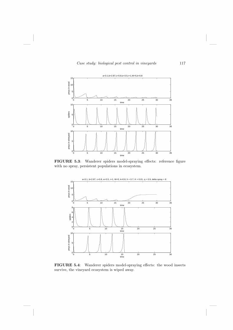
Case study: biological pest control in vineyards 117
0 5 10 15 20 25 30 350
5
10
15
time
prey
s in
woo
d
a=3.1,b=2.87,c=0.8,e=3.5,r=1,W=5,k=0.8
0 5 10 15 20 25 30 350
5
10
time
spid
ers
0 5 10 15 20 25 30 350
5
10
time
prey
s in
win
eyar
d
FIGURE 5.3: Wanderer spiders model-spraying effects: reference figurewith no spray, persistent populations in ecosystem.
0 5 10 15 20 25 30 350
5
10
15
time
prey
s in
woo
d
a=3.1, b=2.87, c=0.8, e=3.5, r=1, W=5, k=0.8, h = 0.7, K = 0.01, q = 0.9, delta spray = 8
0 5 10 15 20 25 300
2
4
6
8
time
spid
ers
0 5 10 15 20 25 300
5
10
time
prey
s in
win
eyar
d
FIGURE 5.4: Wanderer spiders model-spraying effects: the wood insectssurvive, the vineyard ecosystem is wiped away.

118 Spatiotemporal patterns in ecology and epidemiology
0 5 10 15 20 25 30 350
5
10
15
time
prey
s in
woo
d
a=3.1, b=2.87, c=0.8, e=3.5, r=1, W=5, k=0.8, h = 0.7, K = 0.01, q = 0.2, delta spray = 8
0 5 10 15 20 25 300
2
4
6
8
time
spid
ers
0 5 10 15 20 25 300
5
10
time
prey
s in
win
eyar
d
FIGURE 5.5: Wanderer spiders model-spraying effects: entire ecosystemcollapse.
0 5 10 15 20 25 30 350
5
10
15
time
prey
s in
woo
d
a=3.1, b=2.87, c=0.8, e=3.5, r=1, W=5, k=0.8, h = 0.7, K = 0.6, q = 0.04, delta spray = 8
0 5 10 15 20 25 30 350
5
10
time
spid
ers
0 5 10 15 20 25 30 350
5
10
15x 10
33
time
prey
s in
win
eyar
d
FIGURE 5.6: Wanderer spiders model-spraying effects: vineyard pests ex-plosion, all spiders are wiped away.

Case study: biological pest control in vineyards 119
searching for new microhabitats could then be due to the degree of satiationof spiders and to their rejection of certain types of prey.
We keep here the same notation previously used that led to (5.1). In thefirst equation we find again the dynamics of spiders, in which, as before, anegative Malthus growth describes their mortality, and the two nonnegativeterms account for the growth due to predation on the two insect populations.But in contrast to (5.1), here we model the saturation effect the spiders expe-rience when the vineyard insects are too numerous. In such a case, since thewanderers move around and search for other prey in the surroundings of thecultivated land, in the green niches around the vineyards inhabited by the vinsects, a suitable alternative prey source is found. Thus, basing our consider-ations on the field data analysis of Rypstra (1995) and Marc et al. (1999), weuse Holling type II responses to model this feeding saturation effect. Theseterms of course reappear in the appropriate insect evolution equation, but forthe rest the dynamics of all the insect populations considered is the same asin (5.1):
ds
dT= s
(−a +
kbv
H + v+ kcw
), (5.3)
dw
dT= rw
(1− w
W
)− csw,
dv
dT= v
[e− bs
H + v
].
Analysis of the boundary equilibria
The first two feasible equilibria E0 and E1 of (5.1) are found again here,with the same inconditional instability due to the occurrence of the verysame eigenvalues. The equilibrium point E2 instead gets modified as follows:E2 ≡ (s2, 0, v2) =
(ekHbk−a , 0, aH
bk−a
). In this case, it exists only if a < bk, while
for E2 no such restriction arises. The last equilibrium point lying on thecoordinate planes E3 is exactly E3 of (5.1), with of course the same existencecondition a < ckW .
Stability conditions of the last two equilibria differ however from thosederived for (5.1). Notice indeed that for E3, although derived similarly to theformer model, one of the eigenvalues is now 1
H (eH − bs3) while the other twoare the roots of the quadratic Wkcω2 + r(cWk−2a)ω +Wk2cas3 = 0. HenceE3 is stable if and only if br(kcW − a) > c2ekHW and 2a < ckW . Noticethat the presence of the half-saturation constant H renders the satisfactionof the first condition more strict than for (5.1).
The eigenvalues of E2 are r − 1acev2 and those of the matrix
J =1
a(H + v2)2
abkv2(H + v2)− a2(H + v2)2 bekHv2
−abv2(H + v2) ae(H + v2)2 − beHv2
.

120 Spatiotemporal patterns in ecology and epidemiology
Necessary and sufficient conditions for its eigenvalues having negative realpart are tr(J) < 0 and det(J) > 0. Thus E2 is stable if and only if thefollowing conditions are satisfied:
bv2(Hk+H+kv2) > a(v2+H)2, bHev2+(a−e)a(H+ v2)2 > akbv2(H + v2).
Nontrivial equilibrium E4
Now, from the ecological standpoint, of particular interest is the systemequilibrium preserving biodiversity, i.e., ensuring the coexistence of all species.The equilibrium point at which the ecosystem thrives is
E4 ≡ (w4, s4, v4) =(
1be(H + v4),
1br
[W (br − ce(H + v4))], v4
),
and v4 > 0 solves the following quadratic equation:
kc2Wev2 + (abr − kb2r + 2kc2WHe− kcWbr)v+ aHbr − kcWHbr + kc2WH2e = 0.
Two positive roots arise if bckrW < abr+2c2ekWH < bckrW +kb2r, whilethere is only one if abr + kc2WHe < kcWbr. Thus the interior equilibrium isunique and feasible if and only if the latter condition holds and br > ce(H+v4).This gives an upper bound on the location of this root.
For stability, let us analyze once again the characteristic equation at E4,
λ3 + Q1λ2 + Q2λ + Q3 = 0. (5.4)
The coefficients are
Q1 =−bW s4v4 + rH2w4 + 2rHw4v4 + rw4v
24
W (H + v4)2,
Q2 =s
W (H + v4)3[b2kHWv4 − brHw4v4 − brw4(v4)2 + kc2W (H + v4)3w4
],
Q3 =bkw4s4v4
W (H + v4)3[brH − c2WHs4 − c2Ws4v4
].
The Routh–Hurwitz criterion for E4 gives Q1 > 0, Q3 > 0 and Q1Q2−Q3 > 0.Here,
Q1Q2 −Q3 =s4
W 2(H + v4)5·
· [r(kc2Wv4 + A)w24 v
44 + (b2rWs4 + rBw4)w4v
34 + D
],
where A = 5c2kWH−br, B = 10Hc2kW−3br, C = rBH2w24+b2HWs4(rw4−
bkW ), and D = v24C + rAH3w2
4 v4 + rc2kH5Ww24.

Case study: biological pest control in vineyards 121
We then find that Q1 > 0 if and only if
rH2w4 + 2rHw4v4 + rw4v24 > bWs4v4,
Q3 > 0 if and only if
bHr > c2HWs4 + c2Ws4v4,
and Q1Q2 −Q3 > 0 if and only if
Q1Q2 −Q3 ≡ r(c2kWv4 + A)w24 v
44 + [b2rWs4 + w4rB]w4v
34 + D > 0. (5.5)
Sufficient conditions for these conditions to hold are 10c2kWH > 3br andrw4 > bkW . The latter should be satisfied together with the above feasibilityconditions.
Bifurcation analysis
We now investigate the stability behavior of the coexistence equilibrium asa function of the parameter c using a relatively simple method. To ensurethat the characteristic polynomial (5.4) has purely imaginary roots, it musthave the form
(λ2 + Q2)(λ + Q1) = 0, (5.6)
which entails the equality Q1Q2 = Q3 associated to (5.5). Also, a transver-sality condition must hold. Thus a value c = c∗ must exist such that
(i) g(c∗) = Q1(c∗)Q2(c∗)−Q3(c∗) = 0, (ii)d
dcRe(λ(c))|c=c∗ 6= 0. (5.7)
The three roots of (5.6) are η1 = +i√
Q2, η2 = −i√
Q2, η3 = −Q1. In general,however, the roots are functions of c:
η1(c) = β1(c) + iβ2(c), η2(c) = β1(c)− iβ2(c), η3(c) = −Q1(c).
We now verify the transversality condition (ii) of (5.7) at η1 and η2. Substi-tuting the general form of the root ηj(c) = β1(c)+ iβ2(c) into (5.6) and takingthe derivative, we find
K(c)β′1(c)− L(C)β
′2(c) + A(c) = 0, L(c)β
′1(c) + K(c)β
′2(c) + B(c) = 0,
with
K(c) = 3β21(c) + 2Q1(c)β1(c) + Q2(c)− 3β2
2(c),L(c) = 6β1(c)β2(c) + 2Q1(c)β2(c),
A(c) = β21(c)Q
′1(c) + Q
′2(c)β1(c) + Q
′3(c)−Q
′1(c)β
22(c),
B(c) = 2β1(c)β2(c)Q′1(c) + Q
′2(c)β2(c).

122 Spatiotemporal patterns in ecology and epidemiology
Since L(c∗)B(c∗) + K(c∗)A(c∗) 6= 0, we have
d
dc(Re(ηj(c)))
∣∣∣∣c=c∗
=[LB + KA
K2 + L2
]
c=c∗6= 0
and η3(c∗) = −Q1(c∗) 6= 0 so that the transversality condition holds. Thus anondegenerate Hopf bifurcation occurs at c = c∗.
Action of spraying and new simulations
Again human intervention in the ecosystem is modeled via insecticide spray-ing, which in the previous case mathematically corresponded to the additionof Dirac’s delta functions at suitable instances in time to the system (5.1).It is modified here to take into account the fact that poisonous effects of theinsecticide last in time. We assume then an exponential decay of these effectsψ(Ti) = e−α(t−Ti), where Ti ≤ t, i = 1, 2, ..., N denote the spraying instancesfor (5.3). We then get
ds
dT= s(−a +
kbv
H + v+ kcw)− hKqΣN
i=1ψ(Ti), (5.8)
dw
dT= rw(1− w
W)− csw − h(1− q)ΣN
i=1ψ(Ti),
dv
dT= v(e− bs
H + v)− hqΣN
i=1ψ(Ti).
The insecticide efficacy is modeled by the parameter α, with the parametersq, K, h retaining their meaning as for (5.2).
The behavior near the equilibria determined by the theoretical analysis canalso be checked by means of suitable situations. In the absence of spraying,we show in Figure 5.7 the limit cycles obtained with the Hopf bifurcationdescribed earlier. As far as the spraying is involved, general considerations onthe collapsing of the ecosystem or some of its parts entirely similar to the onesof the previous model without saturation (5.1) also hold in this case, despitethe different kind of modeling for the poison’s effects used in this case. But forthis more realistic situation (5.8) with insecticide effects lasting in time, theinsects in the cultivated areas as well as the whole spider population becomeextinct even for very low parameter values.
5.2.1 Models comparison
A major difference between the two proposed models (5.1) and (5.3) isfound in the cycles that can arise in the model introduced here, while theydo arise in the simpler model. This is in agreement with recently collectedvineyard field data, showing persistent oscillations for the spider population(Isaia et al., 2006a).

Case study: biological pest control in vineyards 123
2000 2100 2200 2300 2400 2500 2600 2700 2800 2900 30000
0.5
1
1.5
time
woo
d in
sect
s
2000 2100 2200 2300 2400 2500 2600 2700 2800 2900 30000
100
200
time
spid
ers
2000 2100 2200 2300 2400 2500 2600 2700 2800 2900 30000
50
100
150
a=0.2, b=1.18, c=0.24, e=0.5, k=1, r=1, H=7, W=1
vine
yard
pes
ts
FIGURE 5.7: Limit cycles obtained by the Hopf bifurcation for the Hollingtype II saturation model (5.3).
From the numerical simulations, to maintain stability of the coexistenceequilibrium point, the predation rates must be in an interval with lower andupper bounds respectively depending on the prey in the woods and the preyin the vineyards, i.e., the gap between the parameters b and c should not betoo large. Should this difference be so large that the system oscillates, thestable equilibrium can be reobtained by an increase in the specific growth rateof the prey in the woods, i.e., the parameter r.
The method of spider augmentation led to 60% reduction of pesticide use,Maloney et al. (2003) and the effectiveness of biological control through spi-ders in rice fields and fruit orchards has been documented (Riechert andBishop, 1990; Marc and Canard, 1997; Nyffeler and Benz, 1987). On the otherhand, some insecticides are highly toxic for spiders, for instance, dimethoategives 100% mortality for the lycosid Trochosa ruricola (Birnie et al., 1998)even when applied at lower concentrations than recommended, and methylparanthion and pyrethroid cypermethring are poisons for the genus Erigone(Linyphiidae) (Brown et al., 1994; Huusela-Veistola, 1998).
These field observations should be coupled with our numerical experiments.In the simpler model (5.2) simulations showed that populations can recoverafter spraying if the atmospheric and environmental conditions are not tooharsh. In the ecosystem (5.8), instead, even very low parameter values relatedto human intervention can permanently destabilize the ecosystem. Thus theresults of these models agree with field data. Halley et al. (1996) discoveredthat if spraying is low and less frequently used, spiders can survive, but for

124 Spatiotemporal patterns in ecology and epidemiology
larger quantities of the insecticide or if frequently used, chances are thatthe spider population will be wiped out. This is also documented by themathematical models presented here.
5.3 Modeling the ballooning effect
The model we introduce here differs from the previous ones since in thiscontext spiders are essentially stantial, so that we need to also distinguish thetwo spider populations living in the woods and in the vineyard, respectively,sw(t) and sv(t). We keep the same notation used earlier, but this time wealso assume a vineyard insects carrying capacity V , with V >> W , to modelthe Langhe environment. The model then reads
dw
dT= bw(1− w
W)− `wsw, (5.9)
dsw
dT= −csw + sw[˜w − αw ˜ V
V + W] + svαvk
W
V + W,
dv
dT= av(1− v
V)− kvsv,
dsv
dT= −esv + sv[kv − αvk
W
V + W] + swαw ˜ V
V + W.
Here the first two equations express the fact that insects reproduce logisticallyand are subject to predation by the spiders living in the same environment.The two ecosystems are separate entities, as the web-making spiders tend tolive in the same place, if there is no ballooning effect. Wind transport ofyoung spiders is taken care of in the two equations modeling the growth ofthe spider populations. A fraction α of newborns is carried in the air andmay land either in woods or surrounding vineyards with probability that isassumed proportional to the surface of the two patches, which in turn is relatedto their respective carrying capacities. The last two terms in the spiders’evolution equations describe this migration effect. The last one representsthe immigration of newborns into the woods from the vineyards in the thirdequation and conversely in the fourth equation, while the third terms representthe emigration of wood-born spiders into the surrounding landscape in thethird equation and the opposite way in the dynamics of the vineyard spiders.The predation efficiency of the latter is k. Notice that the transport effect ofthe wind is clearly the same for both species, while it is neglected for insects,as they are able to fly on their own and move toward the environment theyprefer.

Case study: biological pest control in vineyards 125
Boundedness of the solutions
Now we are going to have a look at the properties of the model (5.9). Thefirst step is to check solution boundedness.
The first two equations of (5.9) show that the two insect populations arebounded above:
w(t) ≤ maxw(0),W, lim supt→∞
w(t) ≤ W ; (5.10)
v(t) ≤ maxv(0), V , lim supt→∞
v(t) ≤ V.
Let us also define φ(T ) = w + v + sw + sv. Summing the equations (5.9)for any arbitrary < κ ≤ minc, e, `− ˜, k − k, we have
dφ
dT+ κφ ≤ bw
(1− w
W
)+ av
(1− v
V
)
− (c− κ)sw − (e− κ)sv − (`− ˜− κ)sw − (k − k − κ)sv
≤ bw(1− w
W
)+ av
(1− v
V
)≤ 1
4[bW + aV ] ≡ M .
Then dφdT ≤ −κφ + M , from which Gronwall’s inequality shows that every
population is bounded for all time:
φ(t) ≤ exp(−κt) +M
κ[1− exp(−κt)] ≤ M. (5.11)
Long-term behavior
Now, we need to analyze the system’s equilibria E(i) ≡(w(i), v(i), s
(i)w , s
(i)v
).
The first three, the origin E(0) and the axial points with w(1) = W , w(2) = V ,where the other components are zero, are easily ruled out, since they areunstable. Respectively, we find the eigenvalues
a, b,−c,−e;
a,−b,−e,−c + ˜ W
V + W(V + W − αV );
b,−a,−c,−e + kV
V + W(V + W − αW ).
The first interesting equilibrium is E(3) ≡ (W,V, 0, 0), whose eigenvaluesare −a,−b, and the roots of the quadratic equation
λ2 + λ
[c−W ˜+ e− V k +
αV W (˜+ k)V + W
]
+
(c−W ˜+
αV W ˜
V + W
)(e− V k +
αV Wk
V + W
)− V 2W 2 ˜kα2
(V + W )2= 0.

126 Spatiotemporal patterns in ecology and epidemiology
Sufficient conditions for which the Routh–Hurwitz criterion holds, so thatE(3) is stable, are
c > W ˜, e > V k. (5.12)
The next two are still boundary equilibria, with only one zero component,and in them one of the two insect populations goes extinct. We find
E(4) ≡(
0,e(V + W )
k (V + W − αW ),
a
k
eαW
c(W + V − αW )
[1− e (V + W )
kV (V + W − αW )
],
a
k
[1− e (V + W )
kV (V + W − αW )
])(5.13)
E(5) ≡(
c(V + W )˜(V + W − αV )
, 0,b
`
(1− c(V + W )
˜W (V + W − αV )
),
b
`
V α
e
[c
W + V − αV
] [1− c (V + W )
˜W (V + W − αV )
]). (5.14)
An easy verification based on the fact that 0 ≤ α ≤ 1 shows that the feasibilityconditions reduce respectively to
kV (V + W − αW ) > e (V + W ) , ˜W (V + W − αV ) > c (V + W ) .(5.15)
For the stability analysis, let us calculate the Jacobian of the system J (i) ≡J(E(i)):
b(1− 2w(i)
W)− `s
(i)w 0 −`w(i) 0
0 a(1− 2v(i)
V)− ks
(i)v 0 −kv(i)
(1− α VV +W
)˜s(i)w α W
V +Wks
(i)v (1− αV
V +W)˜w(i) − c α W
V +Wkv(i)
α VV +W
˜s(i)w ks
(i)v (1− α W
V +W) ˜w(i)α V
V +Wkv(i)(1− αW
V +W)− e
.
Thus, for equilibrium E(4), the eigenvalues are −c, b− `s(4)w , and the roots
of the quadratic
λ2 − tr(J(E(4)))λ + det(J(E(4))) = 0, (5.16)
where
J(E(4)) ≡(
a(1− 2 v(4)
V )− ks(4)v −kv(4)
ks(4)v (1− α W
V +W ) kv(4)(1− α WV +W )− e
)(5.17)
≡(
a(1− 2v(4)
V )− ks(4)v −kv(4)
ks(4)v (1− α W
V +W ) 0
).

Case study: biological pest control in vineyards 127
The Routh–Hurwitz conditions for stability are −tr(J (4)) > 0 and det(J (4)) >0, and in view of 0 ≤ α ≤ 1 we find
−tr(J (4)) ≡ ks(4)v − a + 2
a
Vv(4) = ae
V + W
kV (V + W − αW )> 0,
det(J (4)) ≡ kkv(4)s(4)v
V + W − αW
V + W> 0.
Stability of E(4) follows by just requiring
b < `s(4)w . (5.18)
For E(5), the analysis is similar. We find the two eigenvalues, −e, a−ks(5)v ,
and then the eigenvalues of
J(E(5)) ≡(
b(1− 2w(5)
W )− `s(5)w −`w(5)
˜s(5)w (1− α V
V +W ) ˜w(5)(1− α VV +W )− c
)(5.19)
≡ − bc(V +W )
˜W (V +W−αV )−`w(5)
˜s(5)w (1− α V
V +W ) 0
The Routh–Hurwitz criterion yields again
− tr(J(E(5))) =bc(V + W )
˜W (V + W − αV )> 0,
det(J(E(5))) = `˜w(5)s(5)w
V + W − αV
V + W> 0,
and stability of E(5) is ensured by
a < ks(5)v . (5.20)
We analyze sufficient conditions for the existence of the coexistence equi-librium E(6) ≡ E∗ = (w∗, v∗, s∗w, s∗v). Solving the first two equations of (5.9)in terms of w and v, we find
w∗ =W
b(b− `s∗w), v∗ =
V
a(a− ks∗v). (5.21)
For feasibility of E∗ the opposite conditions of (5.18) and (5.20), but bothevaluated at E∗, must hold:
a > ks∗v, b > `s∗w. (5.22)
128 Spatiotemporal patterns in ecology and epidemiology
Let
A ≡ `
b˜ W
V + W(V + W − αV ) > 0,
B ≡ 12[˜
W
V + W(V + W − αV )− c] ∈ R,
C ≡ 12αk
V W
V + W> 0, D ≡ k
a
V W
V + Wkα > 0,
E ≡ `
b˜ V W
V + Wα > 0, F ≡ 1
2˜α
V W
V + W> 0,
G ≡ 12[k
V
V + W(V + W − αW )− e] ∈ R,
H ≡ k
a
V
V + Wk(V + W − αW ) > 0.
Notice that in this context the feasibility of E(4) is equivalent to G ≥ 0,and the one of E(5) corresponds to B ≥ 0. Substitute now (5.21) into the lasttwo equations of (5.9), to get two equations in sw and sv,
−As2w + 2Bsw + 2Csv −Ds2
v = 0, (5.23)−Es2
w + 2Fsw + 2Gsv −Hs2v = 0. (5.24)
Both (5.23) and (5.24) are ellipses in the (sw, sv) ≡ (x, y) plane, bothcrossing the origin. Notice that the origin here in R2 gives for the wholemodel the three equilibria we named E(0), E(1), and E(2). We now study thepossible further intersections of the two ellipses.
The first ellipse with center ( BA , C
D ) and vertices
(B
A± 1
AD
√B2D2 + AC2D,
C
D
)(5.25)
(B
A,
C
D± 1
AD
√A2C2 + AB2D
)
intersects the positive vertical semiaxis at P ≡ (xP , yP ) = (0, 2 CD ) and the
horizontal axis at Q ≡ (xQ, yQ) = (2 BA , 0). Its derivative at the point P is
y′1(P ) = BC , and at the origin it is y′1(O) = − B
C . It is then easily seen to havethe same sign as the abscissa xQ at P , while at the origin it always has itsopposite sign.
Case study: biological pest control in vineyards 129
The second one has center at (FE , G
H ), vertices(
F
E,
G
H± 1
EH
√G2E2 + EF 2H
)(5.26)
(F
E± 1
EH
√F 2H2 + EG2H,
G
H
),
and a further intersection with the positive vertical semiaxis at R ≡ (xR, yR) =(0, 2 G
H ), with the horizontal axis at S ≡ (xS , yS) = (2FE , 0). The derivative
at the point R is y′2(R) = FG
, and at the origin it is y′2(O) = −FG
. It thushas the same sign as the height yR when evaluated at R and opposite signwhen evaluated at the origin. Thus both ellipses have axes parallel to thecoordinate axes.
Four cases of sufficient conditions for the existence of E∗ are obtained fromthe above results:
1A) B > 0, G > 0; here existence and uniqueness of an intersection betweeny1 and y2 in the first quadrant, which gives a feasible E∗ if conditions(5.22) also hold, are guaranteed by either
CH > DG and FA > EB (5.27)
or, alternatively,CH < DG and FA < EB. (5.28)
1B) B > 0, G < 0; we obtain only one condition,
FA > EB. (5.29)
2A) For B < 0, G > 0, the condition now is
CH > DG. (5.30)
2B) For B < 0, G < 0 comparing the derivatives of y1 and y2 at the origin,y′1(O) < y′2(O), we impose an intersection in the first quadrant, in otherwords,
FC < GB. (5.31)
Conditions (5.27) are always satisfied upon substituting the values of A,B, C, D, E, F , G. Indeed, they correspond to requiring c > 0 and e > 0and geometrically to xS ≥ xQ and yP ≥ yR, in which equality holds only forthe cases c = 0 and e = 0, respectively. We find also that (5.29) and (5.30)hold always, together with (5.22). The latter imply that the intersectionE∗ of the ellipses must lie within the square with vertices OPUS, whereU ≡ (xS , yP ) ≡ (2F
E , 2 CD ) ≡ ( b
` ,ak ). But this square is inscribed into the

130 Spatiotemporal patterns in ecology and epidemiology
first ellipse in the cases 1A and 1B corresponding to xQ > 0, i.e., G > 0,so that in such cases E∗ is infeasible since one of the first two coordinates,v, w, is negative. In cases 2A and 2B the arc OP of the first ellipse notcontaining Q lies entirely in the square OPUS and (5.30) and (5.31) guaranteean intersection. It follows that E∗ is always feasible. Figure 5.8 depicts suchsituations.
−0.4 −0.2 0 0.2 0.4 0.67.5
8
8.5
9
9.5
10
10.5
11
11.5
12
a = 1, b = 3, c = 0.1, e= −100, V= 1000, W=10, k=0.1, ktilde=1, ell=10, elltil=10, alpha=0.5
y 1 con
tinuo
us li
ne; y
2 dot
ted
line
−5 0 5−2
0
2
4
6
8
10
12
14
16
A =168.317,Btil =25.1975,C =2.47525,D =0.49505, E =165.017,F =24.7525,Gtil =547.525,H =99.505,
P U
O S
P U
FIGURE 5.8: Illustration of the possible ellipses intersections; on the left,a blowup of the right picture.
Let us look now at some particular cases, starting from e = 0. Two newequilibria then arise, E(0) ≡ (0, 0, 0, sv) for sv ≡ yP ≡ a
b , or also E(1) ≡(W, 0, 0, sv). For c = 0 we find E(2) ≡ (0, 0, sw, 0) and E(3) ≡ (0, V, sw, 0),with sw ≡ b
` . Substituting into the Jacobian, we find the eigenvalues a, b,−c, 0giving instability for E(0) and −b, a − ksv ≡ 0,−c + ˜W (1 − α V
V +W ), 0 forE(1). The stability condition for the latter follows if ˜W (1 − α V
V +W ) < c,i.e., B < 0, or also xQ < 0. Case 2A makes E(1) stable. The eigenvalues ofE(2) are b − `sw ≡ 0,−a, 0, k V
V +W (V + W − αW ) − e. Again, E(2) is stableif G < 0, i.e., for yR < 0, so that case 2A makes it unstable, while case 2B

Case study: biological pest control in vineyards 131
renders it stable. The equilibrium E(3) is always unstable, as the eigenvaluesare 0, a, 0,−e.
Now as e grows, the axis intersection between the ellipses moves away fromthe sv-axis. It retains its stability and thus gives a stable manifold, the arcOP of the ellipse not containing the point Q, where E∗ is located. It can beshown that for e < 0 this is the stable branch of a saddle-node bifurcation ofan infeasible equilibrium. Similar remarks hold exchanging e with c, P withS, and Q with R and reversing the stability concepts.
Condition (5.31) is equivalent to the restriction y′1(O) = − BC < −F
G=
y′2(O), i.e., to FACH > EBGD > EFCD, which yields AE > D
H . Substitutingthe parameter values and simplifying, we obtain (V +W−αV )(V +W−αW ) >V W . From this the true inequality (1−α)(V 2+W 2)+V W (1−α)2 > 0 follows,so that (5.31) always holds. Case 2B always gives a feasible intersection.
Hopf bifurcation
We also analyze in detail this case although the method is similar to theone used for the wanderer spiders models, since it applies here to a fourthdegree equation, and the bifurcation condition (5.35) below differs from theone previously derived for a cubic equation. The characteristic polynomial inthis case is the quartic in λ,
4∑
i=0
biλi, (5.32)
and the following condition ensures that it has purely imaginary eigenvalues:
4∑
i=0
biλi = (λ2 + η2)(λ2 + βλ + ζ) = 0. (5.33)
Expanding and equating coefficients of the same powers gives
b3 = β, b2 = ζ + η2, b1 = βη2, b0 = η2ζ, (5.34)
which in turn are equivalent to the following relationship for the coefficientsof (5.32):
b3b2b1 = b23b0 + b2
1. (5.35)
Let us denote the principal minors of order k of the Jacobian by Mk(J).Assuming that the following sums are taken over all possible principal minorsof the given order, we then find b3 = −tr(J), b2 =
∑M2(J), b1 = −∑
M3(J),b0 = det(J). As a bifurcation parameter we can take e, since it appears onlyin the element J44 with a negative sign, or c appearing only in J33 also withnegative sign. It turns out then that (5.35) is a cubic equation in e:
b3b2b1 − b23b0 − b2
1 ≡3∑
i=0
ciei. (5.36)

132 Spatiotemporal patterns in ecology and epidemiology
To guarantee the existence of a real positive root e†, the signs of the constantterm and of the coefficient of e3 must be opposite. The condition (5.35) canbe rewritten as
tr(J)∑
M2(J)∑
M3(J) = (tr(J))2 det(J) + (∑
M3(J))2. (5.37)
Let M2[J(1:3,1:3)] denote the principal minors of order two of the submatrixJ(1 : 3, 1 : 3) of the Jacobian, formed by its first three rows and columns, anddet[J(1:3,1:3)] be the corresponding determinant. From (5.37) we extract thehighest order terms containing J44, obtaining
J44 · J44[J11 + J22 + J33] · J44∑
M2[J(1:3,1:3)] = [J44]2 · J44 det[J(1:3,1:3)].
The last term (∑
M3(J))2 gives only a contribution to the coefficient of J244
and therefore has not been considered. The coefficient of J344 is thus
c3 ≡ [J11 + J22 + J33][∑
i
M2]− det[J(1:3,1:3)]. (5.38)
The term not containing e is
c0 ≡∑
i
M2[J(1:3,1:3)] det[J(1:3,1:3)] (5.39)
− [J11 + J22 + J33][∑
i
(−1)iM3(Ji4)],
M3(Ji4) being the minor of the element Ji4 in J . The existence condition ofe† > 0 for which (5.33) holds is then
c0c3 < 0. (5.40)
To detect a Hopf bifurcation we need then only worry about the transver-sality condition. The roots of (5.33) are in general of the form
λ1(e) = ξ1(e) + iξ2(e), λ2(e) = ξ1(e)− iξ2(e), (5.41)
λ±(e) =12
[−b3 ±
√b23 −
4b1
b0b3
].
Differentiating the characteristic equation with respect to e and denoting thisby a prime, we get
γ11ξ′1 − γ12ξ
′2 = γ10, γ12ξ
′1 + γ12ξ
′2 = γ20,
where
γ11 = 4ξ31 − 12ξ1ξ
22 + 3β(ξ2
1 − ξ22) + 2(η2 + ζ)ξ1 + η2β
γ12 = 12ξ21ξ2 − 4ξ3
2 + 6βξ1ξ2 + 2(η2 + ζ)ξ2
γ10 = β′(3ξ1ξ22 − ξ2
1) + [(η2)′ + ζ ′](ξ22 − ξ2
1)− ξ1[(η2)′β + (η2)β′]− ((η2)′ζ + η2ζ ′)
γ20 = β′(ξ32 − 3ξ2
1ξ2)− ξ1ξ2((η2)′ + ζ ′)− ξ2((η2)′β + η2β′).

Case study: biological pest control in vineyards 133
On solving for ξ′1 and ξ′2 in the above system, we find
ξ′1 =γ10γ11 + γ20γ12
γ211 + γ2
22
, ξ′2 =γ20γ11 − γ10γ12
γ211 + γ2
22
.
Letting
m†2 =
∑M2[J(1:3,1:3)(e†)], m†
3 =∑
M3[J(e†)]
t† = tr[J(e†)] d† = det[J(e†)],
the transversality condition ξ′1(e†) 6= 0 in terms of the original entries in the
Jacobian matrix is
(d† + m†2)(m
†2t† −m†
3)(t†)4 + 2(m†
3)4[(t†)2 + (m†
3)3] 6= 0. (5.42)
Numerical simulations show that the Hopf bifurcation does indeed arise, sothat sustained oscillations are possible. Figure 5.9 supports our statement.
400 420 440 460 480 500 520 540 560 580 600
0.65
0.7
w=0.648,v=4,sw=2.8,sv=2.995a=1.5,b=1.5,c=0.6,e=0.6,W=10,V=1000,l=0.5,k=2,lt=1.2,kt=0.1,alpha=0.25
time
woo
d in
sect
s
400 420 440 460 480 500 520 540 560 580 6004
4.1
4.2
4.3
vine
yard
s in
sect
s
time
400 420 440 460 480 500 520 540 560 580 6002.7
2.8
2.9
spid
ers
in w
ood
time
400 420 440 460 480 500 520 540 560 580 600
3
spid
ers
in v
iney
ards
time
FIGURE 5.9: Sustained oscillations for the ballooning model (5.9); ecosys-tem survival.

134 Spatiotemporal patterns in ecology and epidemiology
5.3.1 Spraying effects and human intervention
Again we can investigate the results of insecticide spraying, similarly asdone before. Observe that in general the vineyard is assumed to be sprayedfrom planes flying not too high above the ground and aiming at the vineyards,but due to the wind effect the insecticide may land on the woods as well. Alsoas already mentioned, the poison is meant to act on the insects and pests ofthe vineyards, but it may very well affect the spiders, too. Let Ti denote thespraying instants, focusing on the “instant killing effect” of the poison; wethus obtain, as for the wanderer spiders models, the modified model
dw
dT= w
[b(1− w
W
)− `sw
]− h (1− q) δ (Ti) , (5.43)
dv
dT= v
[a
(1− v
V
)− ksv
]− hqδ (Ti) ,
dsw
dT= sw
[−c + ˜w
(1 + α
(− V
V + W
))]
+W
V + Wkvsvα−K (1− q) δ (Ti) ,
dsv
dT= sv
[−e + kv
(1 + α
(− W
V + W
))]
+V
V + W˜wswα−Kqδ (Ti) ,
with parameters that have the same meaning as introduced in the correspond-ing subsection. Again, as the Dirac delta function suddenly pushes downwardthe solutions at the instants Ti, if such perturbation is large enough and ifa basin of attraction of some other stable equilibrium exists, the trajectoriestend toward this alternative equilibrium instead of the former. Thus the hu-man intervention may very well destabilize the ecosystem, as already remarkedin case of the wanderer spiders models.
5.3.2 Ecological discussion
We have discovered that the model presented contains three relevant equi-libria that are conditionally stable, E(3), E(4), and E(5). In both at least onepopulation vanishes. In the second, the wood insects disappear, causing lossof diversity. Thus this equilibrium should be avoided. The situation for E(3)
is even worse, as it ia a spider-free equilibrium, leading to the disappearanceof predators and survival only of possibly harmful insects. E(5) is desirable asit contains no vineyard-living prey. From the farmer’s point of view, it is theequilibrium one should strive for. Finally, looking at the problem from thepespective of the ecologist, E∗ ≡ E(6) shows the whole ecosystem to thrive,which is good for environmental biodiversity.

Case study: biological pest control in vineyards 135
Stability of all these equilibria is always conditional, for E(3) being givenby upper bounds on the woods and vineyard insects’ carrying capacities, forE(4) and E(5) being ensured by keeping both spider populations high enough.
Around the ecological coexistence equilibrium E∗ ≡ E(6) a Hopf bifurcationhas been shown to arise, with sustained oscillations in time for all the modelpopulations. Its consequences may be relevant for the ecosystem, since if theperiodic solutions have too large amplitude, they may end up on one of thecoordinate axes and therefore indicate the disappearance of at least one ofthe species and migration of the solution trajectories of the dynamical systemtoward one of the other equilibria, with possibly unpredictable consequencesfor the environment. This is to be noted, as some external unforeseeablecircumstances, such as fast climatic variations, may very well result in a changeof the spiders’ death rate and lead to such phenomenon.
Similar remarks as for the previous models on the effects of human inter-vention with spraying hold here as well. In the case of a real application, athorough study of the basins of attractions of the various stable equilibria isneeded to find the impact of human intervention.
Field investigations demonstrate that phytophagous pests may have eco-nomically relevant outbreaks after treatments with pesticides that caused areduction of the spiders feeding on them (see, e.g., Birnie et al. (1998), Put-man and Herne (1966), Hukusima and Kondo (1962)), even to become extinctif insecticide is too high or the applications are too frequent (Mansour et al.,1980). The spider population reappears, however, if the interval betweensprayings is sufficiently long.
Much richer and much more complex computer models aimed at the Danishfarmland are those by Thomas et al. (2003), Thomas et al. (1990), Toppingand Sunderland (1994), Topping (1999), and Thorbek and Topping (2005),where the heterogeneous landscape is simulated via a grid of cells for possiblydifferent habitats. Spiders in various states of development are also considered(Topping et al., 2003). All these models, including the ones presented in thischapter, try to provide insights for the management of sustainable agricul-tural systems, using natural predators for pest control, possibly coupled withmeteorological and farming data adapted to the various local conditions.


Chapter 6
Epidemic models
In this chapter we give a brief look at classical epidemics models. For thereader unfamiliar with these topics, this outline is meant as an introductionto some basic terminology, ideas, and equations that will be needed in Chap-ter 7 and in other parts of the book. Among the many review papers that givea more thorough picture of this field, we mention Hethcote (2000). But ofcourse various chapters are devoted to it in several recent and classical books,for instance, Murray (1989), Anderson and May (1991), Brauer and Castillo-Chavez (2001), and Edelstein-Keshet (1988). The natural outcome of thesestudies is the determination of rational vaccination policies to prevent epi-demics outbreaks and to control infectious diseases propagation (Dieckmannet al., 2002).
We illustrate first the basic classical epidemic models, introducing the ter-minology for the various subpopulations involved in the dynamical system.Then some more recent models are presented. In Section 6.3, a structuredmodel is presented in which the biological age is accounted for together withthe development stage reached by the diseased individuals. The final Section6.4 presents a case study on an economically relevant disease affecting farmedanimals.
6.1 Basic epidemic models
Mathematical epidemiology stems from the papers by McKendrick (1926)and von Foerster (1959), at about the same time of the original researches ofLotka and Volterra in population theory.
Basically, these epidemic models partition the population into several dis-tinct classes, accounting for the individuals that may catch the disease, thosethat already are infected and can spread the infection, and those that areremoved from the population. This last class can be formed by the recognizedcarriers, who are then quarantined so that they do not further spread thedisease among the sound individuals, or by the people that have recoveredfrom the disease, or even by those still affected by it but which are no moreable to spread it. An important factor in infectious diseases, the one that
137

138 Spatiotemporal patterns in ecology and epidemiology
mainly motivates the mathematical investigation of the situation, is the factthat very often the infectious people, those who can infect other individuals,are not recognized as being disease affected, since they do not yet have thesymptoms. For instance, people affected by measles and chickenpox can infectother individuals only between the 10th and the 14th days of incubation, andthe 11th and the 14th days respectively, and this occurs well before they arerecognized as disease carriers. Different other possibilities also arise, such asaccounting for an intermediate class of infected but not yet infectious indi-viduals, or individuals that have become infected but for which the diseasehas not yet fully developed, and they are still in a stage preceding the oneof being infectious. Such cases could be modeled for instance by introducingsuitable delays in the differential equations governing the dynamics to simu-late the incubation period of the disease. Later on in this chapter we will alsoconsider a generalization in which age for the individuals and the “stage” ofthe disease are explicitly built into the model.
A second reason for the study of mathematical epidemiology is the devel-opment of meaningful vaccination policies, with the intent of eradicating thedisease. This is possible because the so-called threshold theorems state theconditions under which the disease naturally vanishes.
The diseases we consider at first are the infectious ones, which are transmit-ted upon contact between the infectious and the susceptible individual. Othersituations are possible, such as diseases transmitted by a vector, in general aninsect or a worm, or viral diseases.
Now, we are going to list the basic assumptions leading to the classicalepidemic model (e.g., see Frauenthal, 1980). They are discussed below andwill be further analyzed and removed or changed in the following sections:
a) The disease is transmitted by contact between an infectious individualand a susceptible individual;
b) there is no latent period for the disease, hence a susceptible becomes in-stantaneously infected upon “successful” contact with a disease carrier;
c) all susceptible individuals are susceptible in the same way;
d) the infected individuals are all equally infectious; and
e) the population under consideration is fixed in size, so no demographicsare accounted for in the classical models, this implying that no birthsor migration occur and all the deaths are taken into account.
A final word concerns the outcome of the disease. There are instances inwhich the disease is overcome and the individual remains immune for life, suchas chickenpox, measles, mumps, and rubella. In other instances the individualrecovers from the illness but may catch it again and again, as it happens forexample for the common cold. In still more unfortunate cases, the disease,once contracted, cannot be overcome and is carried for life. AIDS represents
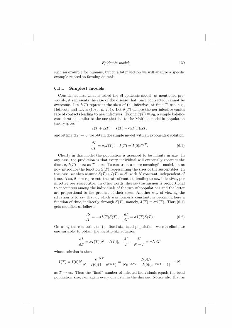
Epidemic models 139
such an example for humans, but in a later section we will analyze a specificexample related to farming animals.
6.1.1 Simplest models
Consider at first what is called the SI epidemic model; as mentioned pre-viously, it represents the case of the disease that, once contracted, cannot beovercome. Let I(T ) represent the sizes of the infectives at time T ; see, e.g.,Hethcote and Levin (1989, p. 204). Let σ(T ) denote the per infective capitarate of contacts leading to new infectives. Taking σ(T ) ≡ σ0, a simple balanceconsideration similar to the one that led to the Malthus model in populationtheory gives
I(T + ∆T ) = I(T ) + σ0I(T )∆T,
and letting ∆T → 0, we obtain the simple model with an exponential solution:
dI
dT= σ0I(T ), I(T ) = I(0)eσ0T . (6.1)
Clearly in this model the population is assumed to be infinite in size. Inany case, the prediction is that every individual will eventually contract thedisease, I(T ) →∞ as T →∞. To construct a more meaningful model, let usnow introduce the function S(T ) representing the sizes of the susceptibles. Inthis case, we then assume S(T )+ I(T ) = N , with N constant, independent oftime. Also, σ now represents the rate of contacts leading to new infectives, perinfective per susceptible. In other words, disease trasmission is proportionalto encounters among the individuals of the two subpopulations and the latterare proportional to the product of their sizes. Another way of viewing thesituation is to say that σ, which was formerly constant, is becoming here afunction of time, indirectly through S(T ), namely, σ(T ) ≡ σS(T ). Thus (6.1)gets modified as follows:
dS
dT= −σI(T )S(T ),
dI
dT= σI(T )S(T ). (6.2)
On using the constraint on the fixed size total population, we can eliminateone variable, to obtain the logistic-like equation
dI
dT= σI(T )[N − I(T )],
dI
I+
dI
N − I= σNdT
whose solution is then
I(T ) = I(0)NeσNT
N − I(0)(1− eσNT )=
I(0)NNe−σNT − I(0)(e−σNT − 1)
→ N
as T → ∞. Thus the “final” number of infected individuals equals the totalpopulation size, i.e., again every one catches the disease. Notice also that as

140 Spatiotemporal patterns in ecology and epidemiology
N → ∞ and σN → σ0 we find I(T ) → I(0)eσ0T , i.e., the model (6.2) in thelimit as the population size becomes infinite recovers the solution of (6.1). Itis also interesting to consider the epidemics curve, defined by how fast thedisease propagates, and this is measured by the rate of change of infectives inthe population
E(T ) ≡ dI(T )dT
=σ(N − I(0))N2I(0)eσNT
[N − I(0)(1− eσNT )]2.
The plots of the solutions and the epidemics curves are contained in Figure6.1.
0 5 10 15 200
100
200
300
400
500
T
I t
0 5 10 15 200
20
40
60
80
100
120
140
T
Et
0 20 40 60 800
20
40
60
80
100
T
I s
0 20 40 60 800
200
400
600
800
T
Es
FIGURE 6.1: Top: trivial model; left: infectives curve I(T ); right: epi-demics curve E(T ); bottom: SI model; left: infectives curve I(T ); right:epidemics curve E(T ).
The reason for which the whole population is ultimately affected is the factthat no individual can overcome the illness. Thus we finally allow the diseaserecovery, and introduce the class of removed individuals R(T ), which comefrom healing the infected at a per capita rate γ. The conservation conditionin this case must then be written as S(T ) + I(T ) + R(T ) = N . The completemodel is then
dS
dT= −σI(T )S(T ),
dI
dT= σI(T )S(T )− γI(T ),
dR
dT= γI(T ). (6.3)

Epidemic models 141
Notice that the infectives equation can be rewritten as
dI
dT= σI(T )
[S(T )− γ
σ
], (6.4)
and therefore the epidemics outbreak, meaning the rapid increase of the in-fective numbers, is avoided and the disease disappears if S(T ) < γ
σ , since thenthe derivative will be negative. R0 ≡ S(0)σ
γ is the basic reproduction numberof the disease; if R0 < 1 then the epidemics vanishes naturally. On solvingformally (6.4) we find
I(T ) = I(0) exp
[σ
∫ T
0
(S(t)− γ
σ
)dt
].
6.1.2 Standard incidence
In all the previous models the basic form of the incidence has been borrowedby the considerations made on chemical reactions (e.g., see Gray and Scott,1990), namely, using the mass action law that takes the rate of encountersbetween the subpopulations to be constant σSI. However, another form isin common use, named standard incidence. The basic idea is the fact thatin a large population one individual cannot encounter all the others all thetime; rather, it meets regularly with a small subset and with a larger numberof people less frequently. The rate of encounters therefore should reflect thisremark, and therefore be an inverse function of the population size. Onceagain, hidden here is the law of diminishing returns. This way of thinkinginvolves then a nonlinearity, and the constant incidence rate now becomesσ ≡ σ(N) = σ0
1N . It thus apparently seems to make things mathematically
worse. However, the contrary happens, as it allows us to reformulate themodel not using the subpopulation sizes but using their fractions. Indeed, letus define
s =S
N, i =
I
N, r =
R
N, s + i + r = 1. (6.5)
To determine their rates of change, observe for instance that the differen-tiation and carrying over the resulting fraction and nonlinear incidence into(6.2) gives
ds
dT=
1N
dS
dT− S
N2
dN
dT≡ 1
N
dS
dT,
ds
dT=
1N
σ(N)IS = σ0I
N
S
N= σ0is.
As we will see, however, the nice property for which the rates of changes ofthe subpopulations S and I and the fractions s and i coincide does not holdin ecoepidemic situations, since in such cases the total population cannot beassumed to be fixed in size. From now on, we identify the constant σ0 simplywith σ. As an application, let us consider the classic SIR epidemic model in
142 Spatiotemporal patterns in ecology and epidemiology
its formulation with sizes (Hethcote, 2000):
dS
dT= µN − µS − σ
IS
N,
dI
dT= σ
IS
N− γI − µI,
dR
dT= γI − µR. (6.6)
Here the first term on the right in the first equation represents the newbornsassumed to be born sound, i.e., belonging to the class of susceptibles. Onintroducing the fractions as indicated above, the model becomes
ds
dT= µ− µs− σis,
di
dT= σis− (γ + µ)i,
dr
dT= γi− µr. (6.7)
With respect to the population models, notice that in (6.7) the dynamics isconfined to the unit simplex, 0 ≤ i + s ≤ 1, i.e., the triangle in the si phasespace with vertices at the origin and at the unit points on the coordinate axes.
For more details on the next considerations, we refer the reader to the re-view by Hethcote (2000). A more general model is the MSEIR model, whichrepresents a transition toward epidemics models including a demographic ef-fect. The class of passively immune individuals M(T ) is introduced, thesebeing the newborns of mothers that in some way have had the disease, andsince they survived it, therefore acquired immunity and transmitted it to theiroffsprings. The newborns of the susceptible mothers are instead still suscep-tible, and therefore belong to class S. A possible transition from class M toclass S is allowed at rate δ. E represents the class of exposed individuals,that are infected but not yet infectious, i.e., cannot spread the disease. If ddenotes the death rate for the population and b its birth rate, the model reads
dM
dT= b(N − S)− (δ + d)M, (6.8)
dS
dT= bS + δM − β
SI
N− dS,
dE
dT= β
SI
N− (ε + d)E,
dI
dT= εE − (γ + d)I,
dR
dT= γI − dR,
dN
dT= (b− d)N,
since now the total population size is not constant, and therefore its dynamicsmust be accounted for. Using fractions with s = 1−m−e− i−r and q = b−d

Epidemic models 143
and introducing the force of infection λ = βi, it becomes
dm
dT= (d + q)(e + i + r)− δm, (6.9)
de
dT= λ(1−m− e− i− r)− (ε + d + q)e,
di
dT= εe− (γ + d + q)i,
dr
dT= γi− (d + q)r,
to be studied in the set (m, e, i, r) : m ≥ 0, e ≥ 0, i ≥ 0, r ≥ 0, m+e+ i+r ≤1. This model has only one endemic equilibrium, E∗ ≡ (m∗, e∗, i∗, r∗)T , with
m∗ =d + q
δ + d + q
(1− 1
R0
), (6.10)
e∗ =δ(d + q)
(δ + d + q)(ε + d + q)
(1− 1
R0
),
i∗ =εδ(d + q)
(γ + d + q)(δ + d + q)(ε + d + q)
(1− 1
R0
),
r∗ =εδγ
(γ + d + q)(δ + d + q)(ε + d + q)
(1− 1
R0
),
where the basic reproduction number is related to the equilibrium number ofsusceptibles,
R0 =εβ
(γ + d + q)(ε + d + q), s∗ =
1R0
.
In this case the force of infection becomes positive if R0 > 1,
λ = δ(d + q)R0 − 1
δ + d + q.
The age structure previously introduced for structured populations in Chap-ter 4 can also be used in the context of epidemiology, as we will see in Section6.3. Here we briefly mention an extension of the MSEIR model with age struc-ture using the fractions, but introduced using the population density U(a, T ),

144 Spatiotemporal patterns in ecology and epidemiology
via relationships of the form, e.g., m(a, T )U(a, T ) = M(a, T ), to get
∂m
∂a+
∂m
∂T= −δm, (6.11)
∂s
∂a+
∂s
∂T= δm− λ(a, T )s,
∂e
∂a+
∂e
∂T= λ(a, T )s− εe,
∂i
∂a+
∂i
∂T= εe− γi,
∂r
∂a+
∂r
∂T= γi,
λ(a, T ) = b(a)∫ ∞
0
β(w)i(w, T )ρe−D(w)−qwdw.
The boundary conditions at age 0 are homogeneous, except
m(0, T ) =∫ ∞
0
f(w)[1− s(w, T )]e−D(w)−qwdw,
s(0, T ) =∫ ∞
0
f(w)s(w, T )e−D(w)−qwdw,
D(a) =∫ a
0
d(w)dw.
Here again a steady state can be calculated, but we just mention the basicreproductive number in this case:
R0 =∫ ∞
0
β(w)ρe−D(w)−qw−γw
∫ w
0
εe(γ−ε)u
∫ u
0
b(χ)eεχdχdudw.
A Lyapunov function can be determined, taking it in the following form,where the coefficients need to satisfy the following relationships:
L(T ) =∫ ∞
0
α(a)e(a, T ) + κ(a)i(a, T )da,
dα
da= ε[α(a)− κ(a)],
dκ
da= γκ(a)− ρβ(a)e−D(a)−qa.
Finally, observe that an average age A of infection can be computed, at theendemic steady state, which for the SEIR and SIR models simplifies to
A = E[a] =
∫∞0
aλ(a)e−Λ(a)−D(a)da∫∞0
λ(a)e−Λ(a)−D(a)da, Λ(a) =
∫ a
0
λ(w)dw.
Many investigations have appeared on vaccination strategies, also in con-nection with models accounting for demographic changes. By way of example,
Epidemic models 145
we mention here only Greenhalgh (1992) and Pugliese (1990), and refer thereader to the bibliography of Hethcote (2000).
Let us finally mention pulse vaccination (d’Onofrio, 2002), in which at fixedtime intervals T∗ a percentage of the population s(nT+
∗ ) = (1 − p)s(nT−∗ ),n ∈ N+ is inoculated and acquires life-long immunity, and therefore migratesto the removed class. The model written for the subpopulation fractions reads
ds(T )dT
= m[1− s(T )]− β(t)si, (6.12)
di(T )dT
= ae(T )− (g + m)i(T ),
de(T )dT
= β(t)s(T )i(T )− (a + m)e(T ),
r(T ) = [1− s(T )− e(T )− i(T )].
Here ρ represents the fraction of vaccinated susceptibles at times Tn = nT∗,n ∈ N+, m is the mortality rate a the inverse latent period of the disease,g is the inverse infection period, and the contact rate β is either constant orassumed to satisfy β(T+1) = β(T ), 1 being the time unit. In d’Onofrio (2002),stability of the limit cycle is investigated, and local and global asymptoticstability conditions of the eradication equilibrium are determined.
6.2 Other classical epidemic models
The model by Capasso and Serio (1978) was prompted by the cholera epi-demics of 1973 in Bari, southern Italy. Here the incidence term in the SIRclassical model is modified to take into account the response the susceptiblesgive when the epidemics starts to spread. Namely, they take measures not tobe infected. This occurs when the number of infectives is high, and therefore itis replaced by a function of I. Two possible choices for the latter are possible.At first we can consider a saturation function, which reaches a saturation levelwith increasing I. But also, to model the psychological response of people,the incidence for low values of I can be taken increasing to a maximum andthen decreasing if I increases further. A possible function that behaves thisway could be provided for instance by the gamma function, g(I) = Ine−αI .The model reads
dS
dT= −g(I)S,
dI
dT= g(I)S − γI,
dR
dT= γI. (6.13)
In Capasso and Serio (1978) results on positivity, global existence, uniqueness,stability, and a threshold-like theorem are shown. The latter states that equi-libria with S ≤ ρ∗ are stable, with ρ∗ = γ
g(0) . For global stability, a Lyapunov
146 Spatiotemporal patterns in ecology and epidemiology
function is explicitly constructed, L(S, I) = I + (S − ρ∗)H(S − ρ∗), whereH(x) denotes the Heaviside function. A further modification is then studied,in which an emigration term for susceptibles is introduced, thereby obtainingthe model
dS
dT= −g(I)S − λS,
dI
dT= g(I)S − γI,
dR
dT= γI + λS. (6.14)
A model that includes a nonlinear incidence is considered in Liu et al.(1986), Liu et al. (1987), in which in simplified form we can write
λ(S, I) = λIpSq. (6.15)
The model considered in Liu et al. (1986) is a SEIRS-type model, whichreads for the fractions of the various subpopulations
dS
dT= −λIpSq + µ− µS + δR, (6.16)
dE
dT= λIpSq − (ε + µ)E,
dI
dT= εE − (γ + µ)I,
dR
dT= γI − (δ + µ)R,
S + E + I + R = 1.
Another model is considered by Beretta and Kuang (1998), in which theinfection is assumed to be caused by a viral agent, and the latter is explicitlybuilt into the system equations. Let P be the viral population and N be thebacterial population that may be infected by the virus, and thus as usual issplit into susceptibles S and infected I. Only the susceptibles are assumedto reproduce according to a logistic equation, with carrying capacity K andto which also the infected contribute in the population pressure term. Thereis a latent period in which the viruses replicate inside the infected bacteria,after which lysis occurs, i.e., the bacteria die and their virus contents, b onaverage, are released into the environment, where the conditions are not idealfor their survival, so that the viral population experiences there a high deathrate µ. The equations then read
dS
dT= rS
(1− N
K
)− λSP, (6.17)
dI
dT= λSP − γI,
dP
dT= γbI − λSP − µP.
It is interesting to note here that upon summation of the right-hand sides,not all terms containing the incidence vanish. Upon rescaling, the system

Epidemic models 147
becomes
ds
dt= as(1− i− s)− sp,
di
dt= sp− `i,
dp
dt= −sp−mp + b`i. (6.18)
The model is analyzed to find that it has only two equilibria, E0 ≡ (1, 0, 0),which is unstable, and the nontrivial equilibrium Ef with all nonvanishingsubpopulations. For the system the set Ω = s + i ≤ 1, p ≤ 1
mb` is shownto be positively invariant. The equilibrium Ef instead is shown to undergo aHopf bifurcation.
6.3 Age- and stage-dependent epidemic system
In this section a step further for modeling the evolution of infectious diseasesis presented, whose basic feature lies in an age description of the populationsunder scrutiny, following what was previously done for an age description ofpopulations. Here we assume that the infection spreads among such structuredpopulation. However, the model is more general than that. In fact, since wehave the possibility of describing the population by age cohorts, we also usethis feature to account for the stage reached by the disease in the infectedindividuals. We therefore use the biological age for individuals, and introducethe “stage” of the disease, counting the time elapsed since contagion, hopefullyup to the recovery. As it is the case for the age-structured populations, theindividuals who just became infected are taken into account via boundaryconditions. The same holds true for those who have just been recognized asdisease carriers.
Before writing the model, we outline the changes needed in the basic as-sumptions of the classical model, previously stated in Section 6.1. Assumptiona will still be maintained. Becoming infected depends on the age of the sus-ceptible; in fact, children and elderly people contract diseases more easily thanindividuals of intermediate age because mature people have stronger naturaldefenses. Thus the age structure in the population removes assumption c.This will be suitably taken into account by the governing equations. To makethe model closer to reality, we also remove assumption b. In the usual delaymodels the incubation period is generally taken as a fixed constant. We in-troduce instead the parameter w to more adequately describe a variable timeincubation period. Thus the elimination of assumption b allows us to modelmore realistically diseases such as measles and chickenpox. The carriers arenot yet recognizable as infected (or infectious), but the ability of spreadingthe disease now is not the same for every individual, so that hypothesis d alsono longer holds. Assumption e will be eliminated at a later stage, recallingthat for the classical epidemics the inclusion of demographic dynamics has led

148 Spatiotemporal patterns in ecology and epidemiology
to more general features (Gao and Hethcote, 1992; Mena-Lorca and Hethcote,1992).
The population we model is described by a nonnegative density n (a, t), afunction with compact support for every t. As we know already from Section4.7, the total population size is
N (t) =∫ ∞
0
n (a, t) da. (6.19)
Let m(a,N) denote the biological mortality of the population; as in Section4.7, it is assumed to be age dependent as well as a function of the total popu-lation size. As in the classical epidemic models, the population is partitionedinto the three distinct classes of susceptibles, infected, and removed individu-als. Again, these are nonnegative functions s, i, and r of their arguments tobe introduced below, with compact support at every fixed time. This parti-tioning is reflected in the following equation, in which the capitalized densitieswill be defined below:
R (a, t) + s (a, t) + I (a, t) = n (a, t) . (6.20)
The density i (a,w, t) gives the number of individuals aged a at time t inthe stage w of the disease, i.e., who were infected w units of time earlier. Itevolves according to
∂i
∂a+
∂i
∂w+
∂i
∂t+ (g (a,w) + m (a,N)) i (a,w, t) = 0. (6.21)
Here g(a, w) represents the rate at which an infected aged a and in stage wof the disease is recognized as a disease carrier and thus migrates into theremoved class. Thus the boundary condition for the latter takes into accountthe contributions over all the incubation periods:
r (a, 0, t) =∫ ∞
0
g (a,w) i (a,w, t) dw. (6.22)
Notice that apparently the disease is not lethal. However, the case of aninfected individual, not yet recognized as a carrier, who dies of the epidemics,will be accounted for as a death in the class of removed individuals in thestage 0 of the recovery.
The total populations in classes r and i are specified as usual by the in-tegral over all possible recovery stages of their respective densities, whichexist by the assumption of n (a, t) being of compact support, since obviouslyi(a,w, t), r(a, v, t) ≤ n(a, t) for every (a, t) and for every w, v, the latter de-noting the recovery period,
I (a, t) =∫ ∞
0
i (a,w, t) dw, R (a, t) =∫ ∞
0
r (a, v, t) dv. (6.23)

Epidemic models 149
Notice also that for w ≥ a, or v ≥ a, the above-mentioned densities areidentically zero, since the stage of the disease, respectively, of the recoveryperiod, cannot exceed the age of the individual.
The only possible outcomes for an individual in class r are either the tran-sition to class s at rate q, or death due to the epidemics at rate z, or thedisease-unrelated death. Thus, similarly to (6.21), we find
∂r
∂a+
∂r
∂v+
∂r
∂t+ (q (a, v) + z (a, v) + m (a,N)) r (a, v, t) = 0. (6.24)
An integration over all the recovery stages of the compactly supported densityscaled via the function z yields the total number of epidemics-related deathsfor individuals aged a at time t,
D (a, t) =∫ ∞
0
z (a, v) r (a, v, t) dv. (6.25)
For the evolution of the susceptibles, notice that, upon recovery, becomingagain a susceptible, an individual aged a still remains aged a at the time ofthe transition. Thus the latter must be accounted for by a nonhomogeneousterm, rather than by a boundary condition. A departure from the susceptibleclass occurs instead only if there is a biological death, or in case of contagion.The very particular case of death immediately following disease contractionis avoided by stating a loss in stage r (a, 0, t). Assumption a of the classicalmodel is used here to write again a homogeneous mixing model. In our case,all the infectives of all ages are assumed to be equally able to spread thedisease, if they are in the same stage. Hence we introduce the quantity
I (w, t) =∫ ∞
0
i (a, w, t) da (6.26)
and find
∂s
∂a+
∂s
∂t+ s (a, t)
(m (a,N) +
∫ ∞
0
p (a,w) I (w, t) dw
)(6.27)
−∫ ∞
0
q (a, v) r (a, v, t) dv = 0.
The function p (a,w) is related to the stage w of the infectives that cause theencounter, and the age a of the susceptible in question. The “new” infectivescome from the interaction term, i.e.,
i (a, 0, t) = s (a, t)∫ ∞
0
p (a,w) I (w, t) dw. (6.28)
To describe the reproduction of the population, thus removing assumptione of the classical model, we consider as in Section 4.7 the age-dependent ma-ternity function b(a,N). However, here we need to state what the effects of

150 Spatiotemporal patterns in ecology and epidemiology
infected individuals are on offsprings. Infected parents can also affect the off-springs, but this might not at all be related to the epidemics in the sense thatchildren of sick parents may not themselves carry the same disease, but mayvery well have other abnormalities. In the human case, this would possiblyoccur to children of a mother infected by rubella, for instance. Taking suchsituations into account is a hard task. We assume simply that only soundindividuals reproduce and at birth newborns are sound. Thus
n (0, t) = s (0, t) =∫ ∞
0
b (a,N) s (a, t) da. (6.29)
Alternatively, every individual can reproduce, but again newborns are sound:
s (0, t) =∫ ∞
0
b (a,N)n (a, t) da.
Suitable initial conditions must complement the above system, that is,
i (a,w, 0) = I0 (a,w) for a > w, (6.30)r (a, v, 0) = R0 (a, v) for a > v,
n (a, 0) = n0 (a) ,
s (a, 0) = S0 (a) = n0 (a)−∫ ∞
0
R0 (a, v) dv −∫ ∞
0
I0 (a,w) dw.
As is the case for the classical models, summing the governing equations(6.21), (6.24), (6.27) and using also (6.20), we obtain the description of thedynamics of the population. The equation governing the evolution of thedensity n (a, t) is then
∂n
∂a+
∂n
∂t+ m (a,N)n (a, t) + D (a, t) = 0, (6.31)
and this allows to deduce that the model is well posed. Notice that this equa-tion differs from the classical Kermack–McKendrick or Von Foerster equationas it contains the migration term, i.e., the total loss due to disease-relateddeaths. To derive the global existence of the solutions, to apply the tech-niques of Gurtin and McCamy (1974) described in Section 4.7 requires us tohandle this migration term. But an upper bound for D (a, t) is easily obtainedfrom (6.20):
I (a, t) , R (a, t) , s (a, t) ≤ n (a, t) (6.32)
for every (a, t), a ≥ 0 and t ≥ 0. The natural hypotheses on the functionsm (a,N) and z (a, v) require them to have a nonnegative infimum for a ≥ 0,v ≥ 0, and N ≥ 0. Also, the maternity function b (a,N) is assumed to beuniformly bounded above for all a ≥ 0 and N ≥ 0. Then the global existenceresult holds for the density n. The same result for the model is deduced from(6.32) and I, R, s being nonnegative.

Epidemic models 151
6.4 Case study: Aujeszky disease
Aujeszky disease (A.D.), caused by the Herpevirus 1 suis (ADV or SHV-1), although not lethal, affects several animal species, among which the hogsconstitute the most relevant one for farmers. This disease is diffused in al-most every European country with relevant economic consequences. In highlydensely populated areas, the Italian law-required control measures are diffi-cult to implement. In northwest Italy, the area of the towns of Villafallettoand Vottignasco in the Cuneo province within a surface of 38 km2 hosts 90000animals in 91 farms with density in some instances over 3500 individuals persquare kilometer. In view of these facts, for modeling purposes we considerthe area as a single giant epidemiologic unit. The seroprevalence droppedfrom the year 1997, in which the new vaccination law was issued, until year2000 to reach the minimum value of 31.5%. Then it went up again to 54.7%in 2004 and afterwards remained stable. The mathematical model consideredhere studies the spread of the disease, with the aim of its eradication, if at allpossible, or at least a reduction of the viral circulation.
The field measures give the following values for the measurable parameters.The size of the epidemiological unit is N = 90000. Data on the positivity ofthe farmed animals have been collected; the average natural mortality of soundanimals is µs = 0.084, the average disease-related mortality is µi = 0.087, andthe average birth rate is ρ = 0.107.
For the remaining parameters appearing in the mathematical model, namelythe disease incidence β and the (absence of) biosafety τ , simulations havebeen performed. Among the latter, biosafety measures play an importantrole. These are represented by devices like continuous fencing of the farm,quarantine stalls, desinfestations, checked visitor access, filtering area betweenthe stalls and other farming areas, and so on.
The disease, once contracted, affects the animal for its life. Hence theepidemics model we consider must be of SI type. The population is partitionedamong the susceptible and infective classes as usual, but reproduces so thatS + I = N , but here the population is not constant, rather N ≡ N(T ). Themodel is then described by the equations
dS
dT= ρN − µsS − β
SI
N− τS,
dI
dT= −µiI + β
SI
N+ τS. (6.33)
The first equation describing the susceptible evolution contains a reproductionterm, coming from the whole population, as also diseased animals reproduce,but all newborns are considered to be sound. It also accounts for the intrinsicnatural mortality µs of the susceptibles, the disease incidence term, and finallya term describing the absence of biosafety measures, for which the disease canbe caught not by direct contact with a sick animal, but by vectors broughtinto the farm by external carriers. Notice that τ = 0 corresponds to the

152 Spatiotemporal patterns in ecology and epidemiology
highest safety measures. The second equation contains the disease-relatedmortality term, and the terms characterizing the new infected individuals:see, for instance, French et al. (1999).
Let us introduce normalized variables. As new variables we take the frac-tions of sound and infected individuals with respect to the total population,
s =S
N, i =
I
N,
so that the population constraint becomes the line
` : s + i = 1. (6.34)
Since the latter is a function of time, the former will also be and their timederivatives have to take this into account. Thus, for instance,
ds
dT=
1N
ds
dT− dN
dT
s
N2=
1N
ds
dT− s
N2(ds
dT+
di
dT)
and similarly for i. Substituting from (6.33), we find
ds
dt= µss
2 + (µi − β)si− (µs + τ + ρ)s + ρ, (6.35)
di
dt= µii
2 + (β + µs)si− (ρ + µi)i + τs.
The equilibria of this system are then given by the equations
µss2 + (µi − β)si− (µs + τ + ρ)s + ρ = 0, (6.36)
µii2 + (β + µs)si− (ρ + µi)i + τs = 0.
These represent conic sections. In principle, they could be studied to deter-mine the flow in the si phase plane, but the advantage of the reduced modelis that in this plane trajectories are confined to the straight line (6.34). Wecan just study then the flow on this “normalized population line” with normaln = (1, 1)T . If it goes up, the angle θ that it makes with n is 0 < θ < π, whileif it is downward, the angle will be π < θ < 2π. To distinguish the two cases,notice that in the former we have sin θ > 0, while the converse situation holdsin the latter. Hence, to calculate the angle θ that n makes with the flow, wecan use the cross product
dxdT
≡(
ds
dT,
di
dT
)T
,dxdT
× n ≡ ‖ dxdT‖‖n‖ sin θ
so that
sgn(sin θ) ≡ sgn(
dxdT
× n)
,

Epidemic models 153
and we are led to study the function
Ψ ≡ sgn(sin θ) = sgn
∣∣∣∣∣∣
i j k1 1 0dsdT
didT 0
∣∣∣∣∣∣≡ ‖k‖sgn
(di
dT− ds
dT
). (6.37)
Upon substitution from (6.36) and (6.34) we obtain the equation Ψ(s) = 0,where explicitly
Ψ(s) ≡ µi(1− s)2 + s(1− s)(2β + µs − µi)+ s(µs + 2τ + ρ)− (1− s)(ρ + µi)− µss
2 − ρ,
which is again a parabola. Recall that when such a function is positive,the projection onto the normalized population line of the flow shows thattrajectories must move upwards toward increasing values of the infectives,i.e., the epidemic propagates. To assess this behavior, it is clearly easier todetermine its zeros first, so that we need to solve the quadratic equation
s2(µi − β − µs) + s(β − µi + µs + τ + ρ)− ρ = 0,
whose solutions are
s1,2 =−(µs + τ + ρ + β − µi)±
√∆s
2(µi − β − µs). (6.38)
These zeros will be real if the discriminant is nonnegative,
∆s ≡ (β − µi + µs + τ + ρ)2 + 4ρ(µi − β − µs) ≥ 0. (6.39)
We need then to determine the region in the βτ parameter space in whichthis inequality is satisfied. Substituting the data for the known parametersand studying the equation corresponding to (6.39), we find
φ(β, τ) ≡ β2 + τ2 − 0.22β + 0.208τ + 2βτ + 0.0121 = 0. (6.40)
To understand its nature, let us consider the matrix of the quadratic form(6.40),
A ≡ (aj,`) =
0.0121 0.104 −0.110.104 1 1−0.11 1 1
, j, ` = 0, 1, 2.
We then investigate the invariants of (6.40):
∆ ≡ detA = −0.045796, δ ≡∣∣∣∣1 11 1
∣∣∣∣ = 0.
Thus φ is a parabola. The slope of its axis is
tan α = −a1,1
a1,2= −1,
154 Spatiotemporal patterns in ecology and epidemiology
i.e., the angle it makes with the s-axis is 34π. The vertex can be obtained by
solving the system
a1,1x0 + a1,2y0 + (a1,1a0,1 + a1,2a0,2)1S
= 0,
[a0,1 + (a0,1a2,2 − a1,2a0,2)
1S
]x0
+[a0,2 +
1S
(a1,1a0,2 − a0,1a1,2)]
y0 + a0,0 = 0,
to give the point (x0, y0) = (−0.031, 0.0253). The intersections with the βcoordinate axis are complex, while with the τ -axis they reduce to a doubleroot, namely, β1 ≡ β2 = 0.11. We also determine the intersections with theline β = 1 to find the equation
τ2 + 2.208τ + 0.7921 = 0
with roots τ1 = −1.757, τ2 = −0.451. There are no real intersections withτ = 1. From these considerations it follows that the discriminant is alwayspositive in the unit square 0 ≤ β ≤ 1×0 ≤ τ ≤ 1. Thus the discriminant∆s(β, τ) ≥ 0 for all 0 ≤ β ≤ 1, 0 ≤ τ ≤ 1 and the roots (6.38) are
s± ≡ s1,2 =β + τ + 0.104±
√(β + τ + 0.104)2 + 0.428(0.003− β)
2(β − 0.003),
always real and distinct. Now, for β > 0.003 we find ∆s < β + τ + 0.104, sothat 0 < s−, s+, while for β < 0.003 we find ∆s > β + τ + 0.104 and thuss+ < 0 < s−. The roots position with respect to the upper bound 1 can bedirectly checked, and the final inequalities we have are 0 < s− < 1 < s+ forβ > 0.003, and s+ < 0 < s− < 1 for β < 0.003.
Remembering that θ is the angle of the flow with the normal to the popu-lation line, then Ψ(s) = sgn(sin θ) ≥ 0 means a downward flow on this line.Also, Ψ(s) ≥ 0 holds always outside the roots interval. Thus, for the case0 < s− < 1 < s+, we have Ψ(s) ≥ 0 for s < s− and conversely, so that trajec-tories approach s−, while for s+ < 0 < s− < 1, we find Ψ(s) ≥ 0 for s− < s,again with trajectories approaching s−. This entails that the only feasibleequilibrium s− is always asymptotically stable. In the population space, thisequilibrium is then
E∗ ≡ (s−, i−) ≡ (s−, 1− s−) (6.41)
≡(−(µs + τ + ρ + β − µi)−
√∆s
2|µi − β − µs| , 1− −(µs + τ + ρ + β − µi)−√
∆s
2|µi − β − µs|)
=(
β + τ + 0.104−√∆s
2|β − 0.003| ,2|β − 0.003| − β − τ − 0.104 +
√∆s
2|β − 0.003|)
,
Epidemic models 155
with ∆s = (β−µi +µs +τ +ρ)2−4ρ|µi−β−µs| = (β +τ +0.104)2− .428|β−0.003|.
Now the goal would be to keep down the level of the infected population,or increase the one of the sound animals. If β → 0, we find
i∗β=0 =0.006− τ − 0.104 +
√(τ + 0.104)2 − .428× 0.0030.006
. (6.42)
This condition is, however, essentially impossible to attain, as it imposesextremely strict measures within the farmed animals since we want to anni-hilate the intramural disease incidence. On the other hand, we could imposebiosafety measures, to eliminate the imported disease carriers, in which caseτ → 0, and we have
i∗τ=0 =2|β − 0.003| − β − 0.104 +
√(β + 0.104)2 − .428|β − 0.003|
2|β − 0.003| . (6.43)
In a more general case, we can try to minimize the surface
i∗ ≡ i∗(β, τ) (6.44)
=2|β − 0.003| − β − τ − 0.104 +
√(β + τ + 0.104)2 − .428|β − 0.003|
2|β − 0.003| .
Note that the restriction of this surface to the coordinate planes is given by(6.42) and (6.43) above. By cutting this surface with planes parallel to thecoordinate ones, we find similar behaviors, namely,
i∗β=h =2|h− 0.003| − h− τ − 0.104 +
√(h + τ + 0.104)2 − .428|h− 0.003|
2|h− 0.003| ,
(6.45)
i∗τ=k =2|β − 0.003| − β − k − 0.104 +
√(β + k + 0.104)2 − .428|β − 0.003|
2|β − 0.003| ,
(6.46)
at “higher” levels. Note that the line β = 0.003 is a removable singularity, asafter simplications the restriction of the surface to that line is described bythe equation
i∗|β=0.003 =τ
τ + ρ.
We can better study the sections of i∗ with τ = k by taking the derivativewith respect to β to find
di∗
dβ
∣∣∣∣τ=k
(β, k) =1
2|β − 0.003|(β − 0.003)[β + τ + 0.104− |β− 0.003|]. (6.47)

156 Spatiotemporal patterns in ecology and epidemiology
Thus, for β > 0.003, the numerator of the partial derivative is τ +ρ > 0 andfor β < 0.003 it is 2β + τ + 0.101 > 0 in the unit square. Thus, the minimumof the surface is to be sought for β = 0. Also, the sections of i∗ with β = hcan be investigated by taking the derivatives with respect to τ . We have
di∗
dτ
∣∣∣∣β=h
(h, τ) =1
2|h− 0.003|
[−1 +
h + τ + .104√(h + τ + 0.104)2 − .428|h− 0.003|
].
(6.48)
On verifying whetherdi∗
dτ
∣∣∣∣β=h
(h, τ) ≥ 0,
we find .428|h − 0.003| > 0, which is clearly always true. Thus i∗β=h(h, τ) isalways an increasing function of τ ; cf. Figure 6.2. Thus the minimum willbe achieved for τ = 0. Combining this information with the former, we justneed to check the value i∗(0, 0) = −0.0613. The fact that at the origin thesurface becomes negative induces us to also investigate the zero level curvei∗(β, τ) = 0. Upon simplification we have
β + τ = 0.003 + |β − 0.003|.
For β > 0.003, we find then τ = 0, while for β < 0.003, the condition givesthe straight line τ = 2(0.003 − β). Below this line, in the small triangle ∇containing the origin shown in Figure 6.3, the infected become negative, i.e.,the infection level drops to zero. This agrees with the findings of Figure 6.2,in which the whole surface over the unit square is shown. In conclusion, thedisease can be eradicated if the two parameters β and τ are pushed downto values contained in ∇. Eradication can be achieved by a combination ofbiosafety measures coupled with measures to contain the horizontal incidenceβ of the disease. These conditions are, however, very difficult to attain, as theyimpose extremely strict measures within the farmed animals since we wantto annihilate the intramural disease incidence. On the other hand, we alsoimpose strict biosafety measures, to eliminate the imported disease carriers.
6.5 Analysis of a disease with two states
In this section we consider an epidemic spreading in a population of fixedsize, a disease that has two states, the recoverable mild form and the strong,possibly lethal one. The population is thus subdivided into three classes: thesusceptibles S, the weakly infected W , and the V strongly affected ones. The

Epidemic models 157
00.2
0.40.6
0.81
0
0.2
0.4
0.6
0.8
1−0.5
0
0.5
1
betatau
FIGURE 6.2: Plot of the surface I∗(β, τ) in the unit square. It becomesnegative near the origin.
0 1 2 3 4 5 6 7 8 9
x 10−3
0
1
2
3
4
5
6
7
8
9
x 10−3
beta
tau
FIGURE 6.3: Contour line i∗ = 0; the surface is negative in the triangle ∇near the origin; compare Figure 6.2 and notice the very small scale O(10−3)on both axes.

158 Spatiotemporal patterns in ecology and epidemiology
governing equations are then
dS
dT= ρS − βSW − (γw + γv)SV + πW + νV, (6.49)
dW
dT= −λW + βSW + γwSV − πW,
dV
dT= λW + γvSV − νV − µV, and N = S + W + V.
The first equation allows reproduction of the susceptibles, whose offspringsare born sound, at the net reproduction rate ρ. It then considers the diseaseincidence β due to contact with weakly infected individuals, producing againonly new weakly infected individuals, and to contact with the strongly affectedones, which, when “successful,” may produce new infected either in the weakor virulent forms, at respective rates γw and γv. Recovery from either infectedstate is in principle possible, although we suppose that the recovery rate πfrom the strong infection is much lower than the one from the mild form ofthe disease, ν. The dynamics of the infected subpopulations is completed byallowing a transition from the milder to the stronger one at rate λ. Finally, thevirulent form may be lethal, and that is accounted for by the disease-relatedmortality rate µ.
Equilibria
The origin is clearly an equilibrium. To find the nontrivial ones, observethat the equilibrium values of susceptibles solve the quadratic
y(x) = βγvx2 − (γvλ + βµ + γvπ + βν + γwλ)x + (λ + π)(µ + ν),
giving
S1,2 ≡ S+,− =(λ + π)γv + γwλ + β(µ + ν)±√∆
2βγv, (6.50)
∆ = ((λ + π)γv + γwλ)2 + β2(µ + ν)2 − 2β(µ + ν)((λ + π)γv − γwλ) > 0,
where the last condition on the discriminant is imposed to have real solutions.In such a case it easily follows that y(0) > 0 and y′(0) = −(γvλ + βµ + γvπ +βν + γwl) < 0 imply that both S1 and S2 are feasible. For the infected, wefind then
V1 =ρ
µS1, W1 =
ρ(λ + π)(µ + ν)βλµ
− ρ((λ + π)γv + γwλ)βλµ
S1, (6.51)
V2 =ρ
µS2, W2 =
ρ(λ + π)(µ + ν)βλµ
− ρ((λ + π)γv + γwλ)βλµ
S2.
Feasibility then requires the following threshold condition for the suscepti-bles:
S ≥ St =(λ + π)(µ + ν)
(λ + π)γv + γwλ,

Epidemic models 159
−3 −2 −1 0 1 2 3 4 5 6 7−80
−60
−40
−20
0
20
40
60
80
100
−7 −6 −5 −4 −3 −2 −1 0 1 2 3−100
−80
−60
−40
−20
0
20
40
60
80
FIGURE 6.4: Possible forms of the function σ3 − Cσ2, C > 0 on the left,C < 0 on the right.
which in turn shows that S1 is infeasible, while S∗ ≡ S2 instead satisfies it.The feasible equilibria are then
E0 = (0, 0, 0), E∗ =(
S∗,ρ(λ + π)(µ + ν)
βλµ− ρ((λ + π)γv + γwλ)
βλµS∗,
ρ
µS∗
).
Stability
The Jacobian of the system is
J = J(S, W, V ) =
ρ− βW − (γw + γv)V −βS + π −(γw + γv)S + ν
βW + γwV −λ + βS − π γwS
γvV λ γvS − µ− ν
.
Now, the eigenvalues at the origin are easily evaluated as σ1 = ρ, σ2 =−λ− π, σ3 = −µ− ν to show that it is inconditionally unstable.
The characteristic equation for E∗ can be written as−σ3+Cσ2+Bσ+A = 0,

160 Spatiotemporal patterns in ecology and epidemiology
0 5 10 15 20 25 300
0.5
1
1.5
2
Sm
time
0 5 10 15 20 25 300
0.5
1
1.5
W
time
0 5 10 15 20 25 300
1
2
3
V
time
FIGURE 6.5: β = 0.1, γw = 0.5, γv = 0.5, λ = 0.3, µ = 0.1, ν = 0.3,π = 0.3, and ρ = 0.4, giving A, B, C < 0 but A + BC 6= 0.
0 5 10 15 20 25 300
0.5
1
Sm
time
0 5 10 15 20 25 300
0.05
0.1
0.15
W
time
0 5 10 15 20 25 300
0.1
0.2
0.3
V
time
FIGURE 6.6: β = 1.0, γw = 1.0, γv = 9.0, λ = 1.0, µ = 3.5, ν = 0.1,π = 0.1, and ρ = 0.5.

Epidemic models 161
with coefficients explicitly given by
A = − ρS2[µβ + γwλ + νβ − 2βS2γv + γvπ + γvλ],
B =1
λµ
[−ρπµ2 − λ2µν − ρλν2 − ρπν2 − λµ2π − ρλ2ν + λµ2βS2
− λµπν + λ2µγwS2 + l2µγvS2 − λµβS22γv + λµβS2ν + λµπγvS2
− ρλνπ − ρλνµ− 2ρπµν − ρπγ2vS2
2 − ρλγ2vS2
2 − l2µ2 + 2ρλνγvS2
+2ρπµγvS2 + 2ρπνγvS2 − ρλµβS2 + ρλγvS22β − ρλγvS2
2γw
],
C = − 1λµ
[l2µ + ρλν − λµγvS2 − λµβS2 + λµν + ρπν
− ρπγvS2 + ρπµ + λµπ + λµ2].
We can seek the eigenvalues as intersections of the two functions Bσ + Aand σ3 − Cσ2, observing that the latter has one of the two forms in Figure6.4. To impose stability, the case C < 0 is the most favorable one, as we needonly to impose also A,B < 0 to have only roots with negative real parts.
0 1 2 3 4 5 6
x 104
0
0.1
0.2
0.3
0.4
Sm
time
0 1 2 3 4 5 6
x 104
0
0.05
0.1
W
time
0 1 2 3 4 5 6
x 104
0
0.05
0.1
0.15
0.2
V
time
FIGURE 6.7: Limit cycle verified over a long time interval: β = 0.003,γw = 0.2, γv = 0.9, λ = 0.1, µ = 0.06, ν = 0, π = 0.1, and ρ = 0.02.
Instead of continuing the analysis in this direction, we concentrate on thepursuit of Hopf bifurcations. To this end, we seek the conditions for whichthe cubic characteristic equation factors into the product of two lower de-

162 Spatiotemporal patterns in ecology and epidemiology
3.6 3.8 4 4.2 4.4 4.6 4.8 5
x 104
0.05
0.06
0.07
0.08
Sm
time
3.6 3.8 4 4.2 4.4 4.6 4.8 5
x 104
0.5
1
1.5
2x 10
−3
W
time
3.6 3.8 4 4.2 4.4 4.6 4.8 5
x 104
0.01
0.015
0.02
0.025
0.03
V
time
FIGURE 6.8: The system dynamics for the same parameters as in Figure6.7 but in long-time simulations: one can readily see persistent oscillations.
0 1000 2000 3000 4000 5000 6000 7000 8000 9000 100000
0.1
0.2
0.3
Sm
time
0 1000 2000 3000 4000 5000 6000 7000 8000 9000 100000
0.05
0.1
0.15
W
time
0 1000 2000 3000 4000 5000 6000 7000 8000 9000 100000
0.1
0.2
0.3
V
time
FIGURE 6.9: β = 0.003, γw = 0.2, γv = 0.9, λ = 0.1, µ = 0.06, ν = 0.005,π = 0.1, and ρ = 0.02.

Epidemic models 163
gree polynomials, so that the following condition must hold in addition toA,B, C < 0:
σ3 − Cσ2 −Bσ −A = (σ2 + α21)(σ − α2) = σ3 − α2σ
2 + α21σ − α2
1α2,
A + BC = 0.
The analysis is then continued numerically. Specifically, for β = 0.1, γw =0.5, γv = 0.5, λ = 0.3, µ = 0.1, ν = 0.3, π = 0.3, and ρ = 0.4, we find a stableequilibrium; see Figure 6.5.
The equilibrium can be slightly destabilized in the transient behavior; Fig-ure 6.6 gives an example of this behavior.
To find persistent oscillations, we now set ν = 0 and β = 0.003, γw = 0.2,γv = 0.9, λ = 0.1, µ = 0.06, ν = 0, π = 0.1, and ρ = 0.02. The results are inFigure 6.7, with a doublecheck on a smaller time range in Figure 6.8.
If we then change the value of ν = 0.001, without changing the otherparameter values, the oscillations are found to diminish in amplitude; seeFigure 6.9.


Chapter 7
Ecoepidemic systems
In this chapter, we begin to consider ecoepidemic models. These are demo-graphic models accounting for interactions among different populations of thetypes described in the preceding Chapter 4 in which a disease also spreads. Toour knowledge, the first papers that appeared in this field are by Hadeler andFreedman (1989), Venturino (1992, 1994), and Beltrami and Carroll (1994).The name of the field is due to Joydev Chattopadhyay, following an earliersuggestion of the late Ovide Arino. Since those first investigations a number ofpapers have appeared in the literature. Among the more recent contributionsto the field, we mention also Chattopadhyay and Arino (1999), Chattopad-hyay et al. (2002), and Arino et al. (2004). In particular these ecoepidemi-ological models turned useful for the analysis of harmful algal blooms, seeChattopadhyay and Pal (2002) and Chattopadhyay et al. (2002; 2003; 2004).Ecoepidemic models involving more complex phenomena among the popula-tions involved have been investigated with more sophisticated mathematicaltechniques in Venturino (2001; 2002; 2004; 2006; 2007), Haque and Venturino(2006a; 2006b; 2007), and Keller and Venturino (2007).
Epidemic models with vital dynamics for the population share the threedimensionality of the dynamical system that we have here (cf. Gao and Het-hcote, 1992), but ultimately the trajectories will lie on a plane in the phasespace, thus allowing the use of classical tools for their study. Unfortunately,this is not the case here.
The chapter is organized as follows. The ecoepidemic models consideredhere contain mass-action incidence, in the various demographic aspects of thissituation. We start from predator prey models in which the disease affects firstthe predators (Section 7.1), then the prey (Section 7.2), and then the othertwo cases of competing (Section 7.3) and symbiotic communities (Section 7.4).
7.1 Prey–diseased-predator interactions
Assume first that the epidemics spreads only among predators and cannotbe transmitted to the prey by interaction. This assumption is biologicallysound for a wide range of diseases. We count only sound prey U , sound
165

166 Spatiotemporal patterns in ecology and epidemiology
predators, V , and infected predators, VI , and in this context the total numberof predators is expressed by the variable P = V + VI . By combining theclassical predator prey model with the mass action SIS epidemic, with thedisease only in the predators we obtain the following model, recalling that allthe parameters are nonnegative:
dU
dT= U
[a(1− U
K)− cV − ηVI
], (7.1)
dV
dT= V [d + eU − fP − δVI ] + (ν + h)VI ,
dVI
dT= VI [k + gU − fP + δV − ν − µ] .
Notice that here prey do not represent the only food source for the preda-tors, since in their absence, and in the absence of the disease, the soundpredators in the underlying classical demographic model do not die out, buttend to the equilibrium value d
f .The first equation gives the dynamics of the prey, the last term account-
ing for the predation process due to infected predators. We split the effectsproduced by sound and infected predators, as their respective rates of preda-tion may be different. Indeed, the parameter η represents a prey loss due tohunting, but, contrary to our basic assumption, it could also mean the “in-stataneous” death of prey by disease contraction. It differs from c since (a)η < c models the situation in which sick predators are less able to catch preyor (b) η > c would denote that the hunting abilities of sick predators maybe unaffected, but prey surviving an attack may catch the disease and die ofit. However, this violates our basic assumption, and then we would need tomodify the model introducing also the infected prey. Situation (a) of reducedhunting efficiency is then assumed having in mind the large predators huntingusing their speed. If disease affected, their running performance would beinferior to sound individuals. We could say that they are able to catch youngor old prey at rate η, but the mature prey not as effectively as they could ifthey were sound. This then justifies condition (a).
The second and third differential equations express the predators’ dynamics.In summing them we find
dP
dT= dV + eUV − fP 2 + hVI + kVI + gUVI − µVI , (7.2)
i.e., the demographics of this whole population, which depends on the sub-populations V and VI . In the second differential equation we find the basicquadratic model for the predators, and the interaction term due to the disease,involving the infected predators VI . The last terms account for the disease re-covery process, which togheter with the former disappear in the sum of (7.2),and the newborns coming from infected predators. The third differential equa-tion contains a similar quadratic model, in this case formulated for infected

Ecoepidemic systems 167
predators (notice the VI term that premultiplies the bracket) and then thedisease process with terms of reversed signs. Here also disease-related deathsare accounted for, expressed by the parameter µ.
We further assume g 6= e, to allow for g > e, that infected predators getmore “reward” from a caught prey, as food may be more valuable for themthan for sound individuals.
Feeding on other sources takes place in both sound as well as diseasedpredators. This occurs at different net rates d, h, and k and the offsprings ofsound individuals are sound, this being expressed by the parameter d, whilethose of infected individuals may be sound, at rate h, or disease affected; thisvertical disease transmission is expressed by the parameter k. Notice that insome instances this is a very reasonable assumption.
Positively invariant sets
We begin to examine the long-term behavior of the model on a simplifiedversion of (7.1), in that we take µ = 0, i.e., biologically we state that thedisease is not that virulent, and furthermore that infected individuals do notreproduce, h = k ≡ 0. An important preliminary question to answer beforedoing any further analysis is possibly to determine conditions for which tra-jectories will remain confined to a compact set, so that they will not “escapeto infinity” i.e., that no species grows without limit.
We outline two theoretical tools for determining positively invariant sets,one geometric and the other analytic.
Geometric approach
This method exploits the following property. Since the system is homoge-neous, the axes and the coordinate planes are solutions. The fundamentalexistence and uniqueness theorem for ordinary differential equations ensuresthen that the trajectories cannot exit from the first orthant. The first ten-tative is to cut out these invariant sets in the three-dimensional phase spaceby using a suitable plane π in the positive cone, i.e., the first orthant in thespace, where U, U, V ≥ 0. It will then be enough to show that the trajectoriesenter the tethrahedron defined by the coordinate planes and by this suitablydefined plane. This means showing that the angle made by the “outward”normal to this plane with the tangent vectors to the trajectories on the men-tioned plane π is larger than π
2 ; see (7.4) below. The outward normal is theorthogonal line pointing away from the origin. This may be a usable methodalso applicable to other cases, for two reasons. Since it gives only sufficientconditions for the existence of such invariant sets, by working differently, attimes we may indeed obtain different conditions under which bounded trajec-tories exist. Moreover, if needed, more complex surfaces might also be used,to possibly give alternative sets of sufficient conditions.
The construction starts from a generic plane in the (U, V, VI) phase space

168 Spatiotemporal patterns in ecology and epidemiology
aU + bV + cVI = d not crossing the origin, d 6= 0, and meeting the positiveorthant a, b, c > 0. Dividing by d we can cast it into the form
π : AU + BV + CVI = 1, A, B, C > 0. (7.3)
This plane has thus the outward unit normal n = (A,B,C). Let the flow ofthe differential system be denoted by x′ = (U ′, V ′, V ′
I ). This plane cuts outof the positive cone a compact positively invariant set if
n · x′|π ≤ 0. (7.4)
See the illustrative two-dimensional Figure 7.1 for a graphical representation,in which the plane π is replaced by a straight line.
0 2 4 6 8 10 120
2
4
6
8
10
12
FIGURE 7.1: For the classical prey–predator dynamical system, the aux-iliary line π : U +V = 10 is shown along with its gradient ∇π = (1, 1) (starredline) and the flow
(dUdT , dV
dT
)(continuous line). The angle of the latter vectors
is obtuse, and if it is on the whole portion of the line π in the first quadrant,the flow enters in the triangle, which is then the positively invariant set.
Ecoepidemic systems 169
Use (7.3) to eliminate VI and obtain
AU[a− a
KU − cV − η
C(1−AU −BV )
]+
B
Cν (1−AU −BV ) (7.5)
+ BV
[d + eU − fV − 1
C(δ + f) (1−AU −BV )
]
+ (1−AU −BV )(
δV + gU − fV − ν − f
C(1−AU −BV )
)≤ 0.
Rewrite (7.5) as follows:
AU
[(a− η
C+
2f
C+
g
A+ ν
(1− B
C
))(7.6)
+ U
(A
C(η − f)−
( a
K+ g
))+ V
(B
C(η − f)− (c + δ − f)
)]
+ BV
[(d +
f − δ
C− f − δ
B+ ν
(1− B
C
))
+ U
(e− g + δ
A
C
)+ V δ
(B
C− 1
)]+ ν
(B
C− 1
)− f
C≤ 0.
If we impose all the above coefficients to be nonpositive, the inequality (7.6)follows. This amounts to satisfying the following system of inequalities, therelative equations of which represent surfaces in the A, B, C space:
S1 : (a + ν)AC + gC + (2f − η) A− νBA ≤ 0, (7.7)
S2 : A (η − f)− C( a
K+ g
)≤ 0, (7.8)
S3 : (f − c− δ) C + B (η − f) ≤ 0, (7.9)S4 : (d + ν)CB + (δ − f) (C −B)− νB2 ≤ 0, (7.10)S5 : (e− g) C + δA ≤ 0, (7.11)S6 : δ (B − C) ≤ 0, (7.12)S7 : ν (B − C)− f ≤ 0. (7.13)
The most complicated inequality to study is the one related to the quadricsurface, i.e., (7.7). All the other ones are “cylinders” with axes parallel toone of the coordinate axes, for which it suffices to study the intersection withthe plane of the remaining coordinates. Let M (1) be the solution set of thecylinders with axes parallel to the A-axis, M (2) be the respective solution setfor the B-axis, and let us denote by M (3) the solution set of (7.7).
The solution set of S7 is a half-space containing also the solution set ofS6. S3 also gives a half-space, but feasibility requires three distinct subcasescorresponding to the signs of the coefficients in the inequality C ≤ f−η
f−c−δ B.The last alternative arising, c+ δ < f < η, indeed gives an empty intersectionwith the first quadrant. We thus require either

170 Spatiotemporal patterns in ecology and epidemiology
a) f > max (η, c + δ) and the slope in the BC coordinate plane must belarger than one, i.e., c+ δ > η must hold, giving in conclusion f ≥ c+ δ.The intersection with the solutions of (7.12) and (7.13) is nonempty.
b) Alternatively, we impose f < min (η, c + δ); the inequality then reversesthe sign, and the intersection with the solution sets of (7.12) and (7.13)is always nonempty, given by the smaller of the two sets, i.e., C ≥max
(1, f−η
f−c−δ
)B.
c) Finally, if the coefficient is negative, η < f < c + δ, the whole firstquadrant of the BC plane is a solution and no additional restrictionsare required.
If nondegenerate, the conic (7.10) is a hyperbola, since the invariant givenby the sum of the products of the coefficients of squared terms with thecoefficient of the mixed product, i.e., − 1
2 (d + ν) − ν × 0, is negative (e.g.,see Bronshtein and Semendyayev, 1964, p. 254). It crosses the origin, withslope 1. Thus a possible nonempty intersection with the solution set of theformer inequalities is possible only if its vertical asymptote lies to the right ofthe C-axis, i.e., the B coordinate of its center is positive, f > δ. Otherwise,a detailed analysis on the slopes of the asymptote and of S6 shows that nocrossings between the two lines are possible.
The condition f > δ found in this case, combined with the alternatives for(7.9), give respectively the possible modified alternatives
f ≥ c + δ > η; δ ≤ f ≤ min (η, c + δ) ; max (η, δ) ≤ f ≤ c + δ. (7.14)
The solution set of inequalities (7.14) is thus the region M (1).
The cylinders with axes parallel to the B-axis are given by S5 and S2. S5
gives half the space as a feasible solution if g > e, a cylinder with axes parallelto the B-axis, while S2 has either the whole first quadrant as a solution forη < f , or an upper section for η > f . In the latter case, combining with S5,we always find the nonempty intersection given by C ≥ max
(δ
g−e , η−fg+ a
K
)A,
the solution set for S5 and S2, i.e., M (2).
Applying together the above conditions, the two sets of cylinders M (1) andM (2) always give nonempty intersections, since they have mutually orthogonalaxes. Thus a feasible solution set for the system of inequalities (7.8)–(7.13)exists.
The quadric (7.7) is in general a hyperbolic paraboloid. Indeed, its invari-

Ecoepidemic systems 171
ants are
∆ ≡
∣∣∣∣∣∣∣∣∣
0 −ν2
a+ν2 f − η
2
−ν2 0 0 0
a+ν2 0 0 g
2
f − η2 0 g
2 0
∣∣∣∣∣∣∣∣∣=
(−gν
4
)2
> 0,
ρ3 ≡ rank
0 − ν2
a+ν2
−ν2 0 0
a+ν2 0 0
= 2,
ρ4 ≡ rank
0 −ν2
a+ν2 f − η
2
−ν2 0 0 0
a+ν2 0 0 g
2
f − η2 0 g
2 0
= 4.
Instead of a complete study of the quadric, we provide conditions to ensurethat the solution set of (7.7) has a nontrivial intersection with the solution setM (1) ∩M (2) of the former ones, (7.8)–(7.13), by investigating the restrictionsof S1 with planes parallel to the coordinate planes.
For A = k > 0, the inequality depends on a straight line, C ≤ k νB+(η−2f)(a+ν)k+g ,
whose ordinate at the origin is positive if η ≥ 2f . This ensures a nonemptyintersection with the solution set M (1). Should this ordinate at the origininstead be negative, an empty intersection with M (1) always exists, as theslope is always smaller than 1, νk
(a+ν)k+g < 1. Combining with (7.14), forwhich the first and last conditions have to be neglected, we obtain the secondequation in (7.15).
Restricting S1 to B = l ≥ 0 gives instead the inequality ruled by the hy-perbola C ≤ A η−2f+νl
(a+ν)A+g . A feasible solution in the first quadrant of theAC plane exists only if η + νl ≥ 2f . But the latter follows from η ≥2f , which is true because it was derived above. The slope at the origin isC ′ (A) |A=0 = 1
g (η − 2f + νl). If it is larger than the biggest of the two slopesof S2 and S5, a nonempty intersection with M (2) can be found. Thus we need1g (η − 2f + νl) ≥ max
(δ
g−e ,aK +g
η−f
). The fractions on the right are positive,
since g > e and η > f . In these conditions, a feasible solution for inequality(7.6) can then be found, thus giving the second equation in (7.15) by pushingdown l to its lower possible bound, l = 0.
In summary, for the SIS model with ν 6= 0, h = 0, k = 0, µ = 0, a compactpositively invariant set exists if the next conditions are satisfied:
g > e, δ ≤ f ≤ min(η
2, c + δ
), (7.15)
1g
(η − 2f) ≥ max(
δ
g − e,
aK + g
η − f
).
172 Spatiotemporal patterns in ecology and epidemiology
Notice that since ν does not appear in the inequalities just found, thesufficient conditions for the existence of a compact positively invariant setfor the SI model with mass action incidence coincide with the above ones.Moreover, since (7.15) are a number of inequalities smaller than the numberof parameters appearing in them, they can be satisfied very likely. But shouldthey be violated, no feasible region found with this method would then exist,i.e., bounded by a plane. It may, however, be provided by the choice of anotherappropriate surface instead of the plane π, still satisfying (7.4). In any case,one should always remember that there are cases when the approach may failto give a suitable set of parameters.
Analytic approach
The approach we are presenting here applies to the model (7.1) withoutthe simplifying assumptions, so that in this paragraph, we can still take h 6=0, k 6= 0, µ 6= 0. Let us define the new function Ψ = U + V + VI , i.e., thetotal population living in the environment. Using κ ≥ 0, and adding κΨ tothe sum of the right-hand sides of (7.1) gives
dΨdT
+ κΨ = χ(U, V, VI) , (7.16)
where we have, recalling that P = V + VI ,
χ(U, V, VI) ≡ (a + κ)U + (d + κ)V + (h + k + κ− µ)VI − a
KU2
− U(cV + ηVI) + U(eV + gVI)− f(V + VI)P
= (a + κ)U − a
KU2 + (d + κ)V + (h + k + κ− µ)VI
+ U [(e− c)V + (g − η)VI ]− fV 2 − fV 2I − 2fV VI .
Assume c > e, η > g to get an upper bound
χ(U, V, VI) ≤ (a + κ)U − a
KU2 + (d + κ)V (7.17)
+ (h + k + κ− µ)VI − fV 2 − fV 2I
= (a + κ− a
KU)U + (d + κ− fV )V
+ (h + k + κ− µ− fVI)VI .
The three parabolas in (7.17) are bounded above by the heights of theirrespective vertices, so that
(a + κ− a
KU)U ≤ (a + K)2
4a= H1, (d + κ− fV )V ≤ (d + κ)2
4f= H2,
(h + k + κ− µ− fVI)VI ≤ (h + k + κ− µ)2
4f= H3,

Ecoepidemic systems 173
and it then follows
dΨdT
≤ −κΨ + (H1 + H2 + H3) ≡ −κΨ + H.
Solving, from Gronwall’s inequality, we find
Ψ(t) ≤ Ψ(0)e−κt +H
κ(1− e−κt) ≤ max
(Ψ(0),
H
κ
). (7.18)
More generally, we could try to study the nature of the function χ on theright-hand side of (7.16), i.e., what kind of quadric surface it is, and determinethe largest point, i.e., the point farthest from the origin. Indeed, such a surfacecan be seen as a level surface of a 4-dimensional hypersurface, the maximumof which will correspond to its largest value.
Equilibria analysis
We now study of the linearized system (7.1) with h = k = µ = 0, near theequilibria, whose superscript in the notation emphasizes that they belong tothe “mass”-action incidence model. We find the following points:
E(m)0 ≡ (U0, V0, VI0) ≡ (0, 0, 0) ,
with eigenvalues a, d, −ν, which show it to be unstable, and
E(m)1 ≡ (U1, V1, VI1) ≡
(af − cdaK f + ce
,ae + a
K daK f + ce
, 0)
,
with the feasibility condition af ≥ cd. The matrix of the linearized systemfactors, to give the eigenvalue
(δ − f)(ae + a
K d)− ν
(aK f + ce
)+ g (af − cd)
aK f + ce
;
the other eigenvalues are the roots of the quadratic polynomial P (µ) ≡ µ2 +µ b1 + b2, with
b1 =aK (fa− cd) + f
(ae + a
K d)
aK f + ce
, b2 =(af − cd)
(ae + a
K d)
aK f + ce
.
Because of the feasibility condition, both coefficients are nonnegative, b1,b2 ≥ 0, implying that, if we exclude particular cases, both roots of thequadratic have a negative real part. The stability condition is thus givenby the negativity of the first eigenvalue, i.e.,
gU1 + (δ − f) V1 < ν. (7.19)

174 Spatiotemporal patterns in ecology and epidemiology
This equilibrium is a focus if the discriminant of the quadratic P (µ) is nega-tive. Notice that for ν = 0, i.e., for the SI case, if feasible, the equilibrium isunstable for δ ≥ f :
E(m)2 ≡ (U2, V2, VI2) ≡
(0,
d
f, 0
),
with eigenvaluesaf − cd
f, −d,
dδ
f− d− ν.
It is stable if af < cd and dδ < f (ν + d).E
(m)3 ≡ (U3, V3, VI3) ≡ (K, 0, 0), with eigenvalues
−a,(ae +
a
Kd) K
a,
(ga− ν
a
K
) K
a,
from which its instability follows;
E(m)4,5 ≡ (U4,5, V4,5, VI4,5) ≡
(0, V4,5, [V4,5 (δ − f)− ν]
1f
).
Here V4,5 solves the quadratic equation φ (V ) ≡ δ2V 2−(df + 2νδ) V +ν2 = 0.For feasibility, observe that since the discriminant reduces to df (df + 4νδ) ≥ 0and φ (0) = ν2 ≥ 0, φ′ (0) = − (df + 2νδ) ≤ 0, φ′′ (0) = 2δ2 ≥ 0, the trinomialhas two nonnegative roots. Thus V4,5 ≥ 0 is ensured. For δ ≤ f , VI4,5 ≥ 0is impossible. Thus δ > f is necessary for feasibility, and VI4,5 ≥ 0 gives a
lower bound on V4,5, i.e., V4,5 ≥ νδ−f . As φ
(ν
δ−f
)= fν
(δ−f)2(fν − d (δ − f)), if
d (δ − f) < fν, for feasibility of both equilibria we need to impose φ′(
νδ−f
)=
fδ−f (d (f − δ) + 2δν) < 0, but the two conditions combined give the contra-
diction 2fν < d (δ − f) < fν; hence both E(m)4,5 are infeasible. For d (δ − f) >
fν we have φ(
νδ−f
)< 0, so that only E
(m)5 is feasible. The eigenvalues of
E(m)5 are then given by
− V5
fν2
[δ2V5 (af + ην)− af (df + 2δν) + ν2 (cf − δη)
]
and by the roots of the trinomial θ (λ) = fλ2 + λθ1 + θ0, θ1 = δ (δ − f)V4,5−(νδ + 2νf + df), θ0 = df ((δ − f) V4,5 + ν) + 2νf (ν − δV4,5). The negativityof the first one is then necessary, again entailing the following lower bound onV5:
V5 >af (df + 2δν) + ν2 (δη − cf) + fην (d + ν)
δ2 (af + ην)≡ r∗.
This can be discussed as above in terms of the trinomial φ. The conditions forthe sign of the remaining ones are algebraically very much involved; only in

Ecoepidemic systems 175
some cases are we able to state some clearcut results. In particular, ν > δV5
is impossible, since φ(
νδ
)= −dfν
δ < 0; we must then have ν < δV5, andthis entails that θ (0) > 0 follows if we require d [V5 (δ − f) + ν] > δV5 − ν.Since the parabola θ (λ) is convex, the case θ (0) < 0 gives immediately theinstability of E
(m)5 . We also obtain that dθ
dλ (0) < 0 for (δ − f) (δV5 − ν) <
(d + ν) f . Letting p∗ = f(ν+d)δ(δ+f) + ν
δ , we have that the sign of dθdλ (0) > 0 is
equivalent to the inequality V5 > p∗. To investigate the latter lower bound,we calculate
φ (p∗) = −f−fν2δ + fdνδ + dνδ2 + 2f2νd + f2d2
(f + δ)2 δ.
Thus, if we require d > δ, it follows φ (p∗) < 0, i.e., the equilibrium is unstable.To impose φ (p∗) > 0, i.e., V5 < p∗, gives the much stronger requirementfdνδ + dνδ2 + 2f2νd + f2d2 < fν2δ. In such a case, however, both rootsof the trinomial θ (λ) are either real and negative, or complex conjugate, butwith a negative real part. In this case, thus, E
(m)5 would be stable.
We find then
E(m)6,7 ≡
(ην + af − V6,7 (ηδ + cf − ηf)
aK f + gη
, VI6,7,
(δ − f) aK V6,7 − ν a
K + g (a− cV6,7)aK f + gη
).
Here the values V6,7 are the roots of the quadratic ψ(V ) ≡ ψ2V2+ψ1V +ψ0 =
0, where
ψ2 = eη (δ − f) + fg (η − c) + δ2 a
K+ c (ef − gδ) ,
ψ1 = δga− eaf − a
Kdf + afg − 2δ
a
Kν − dηg − eην + νgc ,
ψ0 = ν2 a
K− νga .
For the SI model (ν = 0), as ψ0 = 0, V6 = 0 and there is only one nontrivialequilibrium V7 = −ψ1
ψ2. Feasibility for the SIS model, i.e., for the case ν 6= 0,
for U6,7 ≥ 0, gives
V6,7 ≤ af + ην
(c− η) f + δη≡ V ∗ for δη + (c− η) f > 0. (7.20)
No corresponding limitation exists for δη + (c− η) f ≤ 0 and feasibility isalways ensured. We have thus an upper bound on the size of the predatorpopulation. For VI6,7 ≥ 0, we obtain instead the following bounds on the size

176 Spatiotemporal patterns in ecology and epidemiology
of V6,7:
V6,7 ≥aK ν − ag
(δ − f) aK − cg
, fora
Kν ≥ ag,
a
Kδ ≥ f
a
K+ cg, (7.21)
V6,7 ≤ag − a
K ν
cg − (δ − f) aK
, fora
Kν ≤ ag,
a
Kδ ≤ f
a
K+ cg.
Fora
Kν ≤ ag,
a
Kδ ≥ a
Kf + cg, (7.22)
VI6,7 ≥ 0 holds automatically, while for aK ν ≥ ag, a
K δ ≤ f aK + cg, it is impos-
sible. To study the bounds (7.21) we consider the trinomial ψ(V ), from whichwe have a quadratic inequality. Concentrating again only on the discussionof sufficient conditions for feasibility, we assume (7.22) to hold, and consider(7.20). Since in this case ψ(0) = ψ0 = ν
(aK ν − ag
)< 0, there is exactly
one positive root, V7. To satisfy (7.20) it is sufficient to require then thatψ (V ∗) > 0, a condition that reduces to
cf + (2νη + 2aδ + ηd)νc
ad+
η2νδ
af< η (f − δ) +
η2ν
d+
1ad
(aδ + νη)2 +ν2c2
ad.
(7.23)
Thus (7.22) and (7.23) ensure the feasibility of E(m)6 . An alternative ap-
proach for feasibility consists in assuming both U(m)6,7 and V
(m)I6,7 to be feasible,
i.e., (7.22) and the inequality
ηδ + (c− η) f ≤ 0. (7.24)
Then no restrictions on the size of V(m)6,7 are necessary, and we need only to
require the latter to be nonnegative. This can be achieved by observing thatthe quadratic form ψ (V ) possesses at least one positive root. Since ψ (0) < 0,it is enough to require ψ′′ > 0, which gives
ψ2 > 0. (7.25)
We do not study the stability of this equilibrium point.
7.1.1 Some biological considerations
Our analysis has shown some sufficient conditions on the parameters en-suring the boundedness of the system trajectories; interestingly, they are in-dependent of the parameters a, d. Thus net reproduction rates do not affectthe existence of this invariant set.
Also, since the conditions do not depend on ν, the positive invariant setexists for both the SIS (ν > 0) and SI (ν = 0) models. Geometrically, the net

Ecoepidemic systems 177
reproduction rates push the trajectories of the dynamical system away fromthe origin, but this effect in a sense disappears far away from the origin, a factreflected by their absence from the sufficient conditions giving the invariantset.
Notice also that the condition g > e is necessary, in this analysis, for theexistence of the invariant set. For g ≤ e, indeed, condition (7.11) becomesimpossible and thus the existence of the invariant set is not ensured. However,by rearranging the grouping of terms, another existence proof might be set up.The boundedness of the f parameter in (7.15) shows that the “competition”term in the predators must not be too low, since it exceeds the infection rateof the disease, δ, but also not too large, being limited by the returns in huntingc and η obtained by sound and diseased predators.
The points Em0 , Em
1 , Em2 , Em
3 correspond to the equilibria of the underlyingdemographic model, and therefore are biologically important as being diseasefree. The origin remains an unstable equilibrium also in the ecoepidemicmodel. The same feasibility condition for the demographic equilibrium E1,which is also globally asymptotically stable, also holds for Em
1 , but the latteris stable only if the additional condition (7.19) holds.
As for the prey–predator model, Em2 is stable when Em
1 is infeasible, butin the ecoepidemic model another condition must be satisfied δd < f (ν + d),which for the SI model (ν = 0) becomes δ < f . Em
3 is unstable as its under-lying demographic counterpart.
In the ecoepidemic model there are also new equilibria not appearing in theclassical prey–predator model. No prey survive at Em
4,5. Notice that Em5 is
feasible for δ > f , i.e., when E2 of the classical model is unstable. To makeEm
5 unstable, the level of the predator equilibrium population, V5, should notexceed the ratio of recovery to contact rates, namely, ν
δ . But this is impossiblefor the SI model (ν = 0). If V4 and V5 do not exceed the quantity ν
δ−f , bothequilibria Em
4,5 are infeasible.Feasibility for equilibria Em
6,7 is very difficult to be interpreted biologically.But combining the two inequalities (7.22) we find again δ > f , so that oncemore feasibility is related to the instability of the prey–predator equilibriumE2.
The disease is endemic at Em5 , but the prey are also wiped out. If the goal
is the eradication of an obnoxius pest, one could introduce a diseased predatorin the ecosystem and aim for Em
5 . But the same result could be achieved inthe classical prey–predator model by striving for equilibrium E2. Thus theintroduction of the disease seems to be useless.
Let us now attempt a partial answer to one biologically relevant question,namely, whether the introduction of a prey can eradicate a disease spreadingin the predators. From Em
4,5, in case of the SI model, ν = 0, we find that E(m)4
migrates to the origin, which as we know is always an unstable equilibrium,but we also have V
(m)5 = df
δ2 , from which it follows V(m)I,5 ≥ 0 for δ ≥ f . Thus

178 Spatiotemporal patterns in ecology and epidemiology
Em5 is feasible, with eigenvalues
1δ2
[δ (aδ − dη) + df (η − c)] ,[−f ±
√f (5f − 4δ)
] d
2δ.
They have negative real parts if dη > aδ, c > η, 4δ > 5f . Thus the introduc-tion of the prey, although they in the end disappear, causes the predators topartly survive the epidemics unaffected, since part of the population survives,at V
(m)5 > 0. Comparing with the SI epidemics model, for which all individu-
als ultimately become infected, the presence of the prey acts as a “recovery”from the disease, i.e., what the SIS model prescribes. The prey thus allowsthe survival of a part of the predator population unaffected by the disease.
We conclude the Section by mentioning a result on the more general modelallowing disease-related deaths. For small values of µ the behavior near theinterior endemic equilibrium is similar to the one seen above, but increasingits value moderately, a bifurcation occurs; see Figures 7.2 and 7.3. Increasingit further however, the persistent oscillations disappear and the trajectoriestend to a different (boundary) equilibrium.
7.2 Predator–diseased-prey interactions
We now consider the disease spreading among the prey. We count soundprey U , infected prey UI , and sound predators V . Since the epidemics spreadsonly among the former, the system takes the form
dU
dT= U [a− bU − cV − λUI ] + γUI , (7.26)
dUI
dT= UI [λU − kV − γ],
dV
dT= V [d + eU − fV − hUI ].
The equations state that the disease can be overcome at rate γ. The sign ofh is understood to be undetermined, to describe interactions possibly leadingto quick deaths of predators upon contact, h > 0, or predators hunting ofinfected animals occurs at a different rate h < 0 than the one for sound prey.
Let us examine the boundedness of the system trajectories first. Proceedingfrom the easier SI model, if h > 0, the set [0, U]× [0,∞)× [0, V ], U ≥ a/b,d + eU − fV ≤ 0, is positively invariant in the U UI V space.
Indeed, it suffices to determine the sign of dUdT and dV
dT , deleting the terms−λUI and −hUI from the equations (3.1). The given conditions ensure thatU ′ < 0 on U = U, while the one for V states that the point (U, V ) liesin the region V ′ < 0.
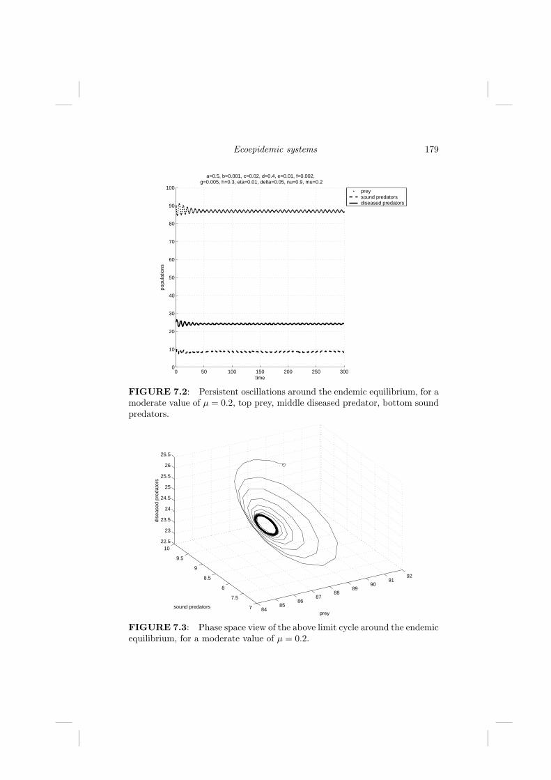
Ecoepidemic systems 179
0 50 100 150 200 250 3000
10
20
30
40
50
60
70
80
90
100
popu
latio
ns
time
a=0.5, b=0.001, c=0.02, d=0.4, e=0.01, f=0.002, g=0.005, h=0.3, eta=0.01, delta=0.05, nu=0.9, mu=0.2
preysound predatorsdiseased predators
FIGURE 7.2: Persistent oscillations around the endemic equilibrium, for amoderate value of µ = 0.2, top prey, middle diseased predator, bottom soundpredators.
8485
8687
8889
9091
92
7
7.5
8
8.5
9
9.5
1022.5
23
23.5
24
24.5
25
25.5
26
26.5
preysound predators
dise
ased
pre
dato
rs
FIGURE 7.3: Phase space view of the above limit cycle around the endemicequilibrium, for a moderate value of µ = 0.2.

180 Spatiotemporal patterns in ecology and epidemiology
For h < 0 and b > k, instead, an invariant set is given by the finite partof the positive cone cut out by the plane π : AU + BUI + CV = 1, whereA,B, C > 0 satisfy
aAB + λ(B −A) < 0, λA < B(c + λ), hA < B(λ− e); (7.27)dCB − (kB + hC) < 0, λC < B(b− k), hC < B(f − k).
Now we must also consider the term −hUI , but working with the plane πas above, imposing that its normal n ≡ (A,B, C) makes an obtuse angle withthe flow x ≡ (U,UI , V ), we must then have n · x′|π < 0. This becomes
UA[(aAB + λ(B −A))(AB)−1 + V/B(λC + (k − b)B)+U/B(λA− (c + λ)B)] + CV [(dCB − (kB + hC))(CB)−1
+V/B(hC + (k − f)B) + U/B(hA + (e− λ)B)] < 0.
It is enough to require that each coefficient be negative, i.e., this amountsto (7.27). Geometrically they mean an intersection of a hyperbola with twostraight lines. For the first equation in (7.27), the hyperbola has a verticalasymptote at B = λ/a and slope at the origin A′(0) = 1. As the slope of thefirst line is larger, no other conditions must be imposed. For the second line,no other restriction is necessary in the cases λ < e and λ > e, since in boththese cases there will be a nonempty intersection with the solution set of thefirst inequality.
For the second equation in (7.27), instead, the pole for the hyperbola liesin the left half-plane, and its slope at the origin is C ′(0) = −k/h > 0. Thelinear inequalities can be rewritten as follows:
C < (b− k)/λ B, C > (f − k)/h B.
We need to require the slope of the first line to be positive so as to find asolution for the system, i.e., b > k, while the second one always admits anintersection with the solution of the quadratic inequality.
We explore now the existence of positively invariant sets for the SIS model,exploiting the idea of the SI model. For the plane σ : AU + BUI + CV = 1,we have here
n · x′|π ≡ UA
B[(aB − (λ + γA)) + U((λ− γ)A− (b + λ)B)
+ V ((k − c)B + (λ− γ)C)] +γ
B(A− 1)
+ VC
B[U((e− λ)B + (h− γ)A) + (γ(1−A) + dB
+ (γ − h)) + V ((k − f)B + C(h− γ))]− kV < 0.
Dropping −γA in the next to the last bracket gives the two systems ofinequalities in the BC parameter plane:
(k − c)B + (λ− γ)C < 0, dCB + (2γ − h)C − kB < 0, (7.28)(k − f)B + (h− γ)C < 0,

Ecoepidemic systems 181
and in the AB parameter plane:
B < A(λ + γA)/(λ + aA), (λ− γ)A− (b + λ)B < 0, (7.29)(e− λ)B + (h− γ)A < 0, A < 1.
Examining in detail all possible situations, we are led to the following set ofinequalities, giving ranges for the parameters for which (7.28) and (7.29) havesolutions. Namely, (7.28) is solvable for h > 2γ if either
f > k > c,γ − λ
k − c>
h− γ
f − k, γ > λ
ork < min(c, f)
hold. For 2γ > h > 0 solutions exist by picking one set of conditions fromeither
f > k > c, γ > λ,γ − λ
k − c<
h− γ
f − k
ork < min(c, f),
and a second set from either
k > c, γ > λ,2γ − h
k<
γ − λ
k − c
ork < c.
Finally, for h < 0 we need
k > f,γ − h
k − f>
2γ − h
k,
and one set from either
k > c, γ > λ,2γ − h
k>
γ − λ
k − c
ork < c.
The system (7.29) possesses solutions if we take one set of conditions fromeither
e < λ, γ < h, γ − h < e− λ,
ore > λ.
The parameter ranges giving solutions for the system (7.28) need to bepaired then with those solving the system (7.29). In particular, notice that

182 Spatiotemporal patterns in ecology and epidemiology
a set of easily understandable sufficient conditions are given by h > 0, k <min(c, f), e > λ. Thus the system trajectories are bounded in the case of thediseases prey having a strong impact on the predators, if the predation rateon infected prey is less than both the predators’ logistic pressure term andthe hunting rate on the sound prey, and the conversion rate of the predatorsexceeds the disease incidence.
For h < 0 some sufficient conditions for the existence of a compact posi-tively invariant set are given, for instance, by c > k > f , e > λ, which areeasily interpretable as suitable rates in the model, and the more complicatedcondition involving also the recovery rate of diseased individuals:
γ(k − f) < f(γ − h).
Equilibria and their stability
The origin is easily found to be the first of the equilibria Ei ≡ (Ui, UI,i, Vi).E0 ≡ O has eigenvalues a, −γ, d, and thus it is unstable.
Then we have E1 with only a nonzero component given by V1 = df . Its
eigenvalues are −c df + a, −k d
f − γ, −d. It is locally asymptotically stablethen if fa < cd. Another equilibrium with only a nonzero component is E1,with U2 = a
b . The eigenvalues are −a, λab − γ, 1
b (db + ea), thus is it alwaysunstable. The next equilibrium is the one corresponding to the demographicmodel without disease. Letting D = bf + ce, it is E3 with U3 = 1
D (af − cd),UI,3 = 0, V3 = 1
D (db + ea). It is feasible for af ≥ cd. One eigenvalue can beexplicitly evaluated as [(af − dc)λ− k(db+ ea)]/D− γ; the other ones are theroots of the quadratic T (µ) ≡ µ2 + µ b1 + b2, with
b1 = − t1D
, b2 = − t3D
,
t3 = (db + ea)(dc− fa),t1 = −fa(b + e) + bd(c− f).
Explicitly, they are given by
T1,2 = [2(ce + fb)]−1[t1 ± t1/22 ], t2 = t21 + 4t3(bf + ce).
The feasibility condition U3 > 0 implies t3 < 0, so that t2 < t21. Hence bothroots of the quadratic have a negative real part. Stability is thus ensured bynegativity of the first eigenvalue, λU3 < kV3 + γ.
The equilibrium E4 with all nonnegative components is analyzed only forthe SI model, γ = 0. Here
V4 =λ
kU4, UI,4 = −Z
∆, U4 = Ψ
k
∆, Ψ ≡ λd− ah,
∆ ≡ λ(λf − hc)− k(bh + λe), Z ≡ λ(dc− fa) + k(db + ea).
Ecoepidemic systems 183
Feasibility gives either
Ψ > 0, ∆ > 0, Z < 0, (7.30)
orΨ < 0, ∆ < 0, Z > 0. (7.31)
The characteristic polynomial is Ξ(µ) = µ3 + a1µ2 + a2µ + a3 with
a1 =Ψ∆
(fλ + kb), a2 =Ψ∆2
kλ[Z(h− λ) + ΨD], a3 = −k
(Ψ∆
)2
λZ.
The Routh–Hurwitz criterion gives the following results. If (7.30), then botha1 > 0 and a3 > 0 are consequences of the existence assumptions and thestability requirement follows if and only if a1a2 > a3, i.e., explicitly,
(fλ + bk)[DΨ + Z(h− λ)] + Z∆ > 0. (7.32)
For the case h < 0, we can restate it, since the last two terms are equivalentto
Z[(fλ + bk)(h− λ) + ∆] ≡ Z λ[h(f − c)− k(b + e)].
Then it suffices to ask f > c for (7.32) to hold. If (7.31) are satisfied, thenagain a1 > 0 follows from the feasibility, but a3 > 0 contradicts the assump-tion Z > 0. Thus (7.31) never give stable equilibria.
Notice that the equilibrium E4 for the SIS model splits to give rise to a pairof equilibria.
Finally, note that for the SI model γ = 0, we also have the following extraequilibrium, E∗ ≡ (U∗, UI,∗, V∗) ≡ (0, UI,∗, 0), with an arbitrary value forUI,∗. The eigenvalues are a−λUI,∗, 0, d−hUI,∗. The trajectories then lie onthe plane UI = UI,∗. The equilibrium is locally asymptotically stable if UI,∗is large enough, i.e., for a
λ < UI,∗, dh < UI,∗.
Summary of findings
In this model, the instability of the equilibria E0, E2 is inherited from thecorresponding equilibria of the underlying predator prey system. The otherequilibrium E1 on the coordinate planes of the U UI V space is stable if andonly if the corresponding point of the underlying prey–predator model is in-feasible. Also, E1 is stable exactly as the underlying demographic equilibrium,and this occurs if and only if E3 is infeasible. Notice that a general featureof ecoepidemic models is that the interior equilibrium of the classical modelbecomes a boundary equilibrium in the ecoepidemic model, since it lies onone of the the coordinate planes of the phase space. In this case it is the pointE3.
The model also possesses the nontrivial equilibrium E4, in which the diseaseis endemic. The two species survive at a different level than prescribed by the
184 Spatiotemporal patterns in ecology and epidemiology
underlying demographic model. For stability, the analysis gives the followingsufficient condition. The crowding effect of predators should be larger thanthe predation rate on prey dynamics, at least for the case when the predatorsdo not contract the disease. In addition, the level of both populations canbe different than the prescribed values at the nontrivial equilibrium of theclassical model by imposing that
λΨ∆6= db + ea
D, k
Ψ∆6= af − cd
D.
These are two extra conditions, we already have another three given by (7.30)to ensure existence, and one more for stability, (7.32). Overall, then, thereare six conditions to be satisfied, with nine parameters, as γ = 0 here. We canthus conjecture that for a suitable selection of the parameters of the model,the equilibrium is feasible, stable, and at a level not prescribed by the classicalprey–predator model. Thus the disease in the prey acts as a controller for thesize of the predators. In particular, for the case of pest control, the parameterscould be chosen so that the prey equilibrium is at a smaller level than the oneprovided by the classical model.
7.3 Diseased competing species models
In the literature [e.g., see Begon and Bowers (1995a), Holt and Pickering(1986) and the bibliography cited therein] models of competition type havebeen treated and the role of multispecies interactions discussed, where thehost density is itself considered as a dynamical variable, and an “ecological”perspective is envisaged. An investigation of two exponentially reproducingpopulations, each of them affected by the disease, can be found in Holt andPickering (1986). Coexistence is governed by inter- and intra-specific infec-tions. The numerical simulations do not reveal stable limit cycles. At thesame time, the complications of the theoretical analysis of the stability arestressed. This fact will also be reflected in this section, in which the mostcomplicated equilibria are essentially intractable, and therefore investigatedmainly by numerical means.
In Holt (1977) a comparison with the Lotka-Volterra model with apparentcompetition among the hosts is discussed. The main inferences state that theprevalence of infection does not depend on alternative species being present;stable coexistence is impossible for a disease spreading only among the hostspecies. In Begon and Bowers (1995b) two species share an infective agent, andlimit cycles are discovered around the equilibrium whose stability is regulatedby inter- and intra-specific infections. However, a whole range of possiblecomplex behaviors is found. The system is also examined from an ecological

Ecoepidemic systems 185
viewpoint, i.e., allowing one of the hosts to be a pest that the pathogen issupposed to fight.
Closely related to the present investigation are the competing systems witha disease-free species together with another epidemics-affected host, which areconsidered in Begon and Bowers (1995a). The classical paper by Andersonand May (1986) considers two competitors, of which one is disease affected.The effect of the latter is to forbid reproduction of the infected individu-als. The results highlight the possibility that the epidemics-affected superiorcompetitor that if unaffected, would eliminate the other competitor, settlesinstead toward coexistence with it.
Two pathogens “competing” over the same host have been considered forinstance in Dobson (1985) and Hochberg et al. (1990). Hochberg and Holt(1990) demonstrates that coexistence is allowed at an intermediate level be-tween the efficient exploitation of the infected hosts and the less virulentexploitation of healthy ones.
We consider two species whose sizes at time T are denoted by P (T ) andQ (T ). They may represent two predators feeding on each other, or two speciesin the same habitat using the same resources, for instance, goats and cattlegrazing on the same meadows. We take the Q species to be affected by anepidemic, which cannot be transmitted to the P population, indicating by QI
the infected Q’s. The model with mass-action incidence and the possibility ofdisease recovery is
dP
dT= P [a− bP − cQ− ηQI ] , (7.33)
dQ
dT= Q [d− eP − f (Q + QI)− δQI ] + νQI ,
dQI
dT= QI [δQ− gP − f (Q + QI)− ν] .
Each equation describes the logistic growth for the P and the Q species;it contains the negative cross-product interaction terms whose negative signdescribs competition. The last equation gives the dynamics of the diseasedpopulation, which is less able to compete for resources, this being describedby the different parameter η in the first equation.
Local stability analysis
Some biologically important questions that can be answered in part bythe stability analysis concern the possibility that the action of a competitorin an environment in which an epidemic spreads among a population mighteradicate the disease, if and how a disease can push to extinction one of thecompeting species, and under what circumstances the disease creates unstabledynamics.
The equilibria Ei ≡ (Pi, Qi, QI,i) of the system are the following alwaysfeasible points: the origin E0 with eigenvalues a, −ν, d, giving instability; E1

186 Spatiotemporal patterns in ecology and epidemiology
with only a nonzero component P1 = ab and eigenvalues −a, − 1
b (ag + bν),1b (bd − ae), showing it is stable if ae > bd; E2 again with only one nonzerocomponent, Q2 = d
f , with eigenvalues −d, 1f (af − cd), 1
f (dδ − df − fν) andstability conditions
cd > af, f (ν + δ) > dδ. (7.34)
These points are the corresponding phase space equilibria of the underlyingdemographic model, also with similar stability conditions. Only for E2 doesan extra condition on the epidemiological parameters arise (7.34) showingthat the disease then affects the infected species dynamics. Considering theSI model ν = 0, (7.34) reduces to f > d, i.e., it gives an extra demographiccondition on the model. Thus, disease introduction may alter the stabilityof E2 simply since f < d destabilizes the otherwise stable equilibrium in thedisease-free environment, for cd > af . It also helps the weaker species ifit is introduced in the “winning” species, as the former would thrive in anecosystem where normally it is wiped out by the adversary competitor.
The role of (7.34) is important also from the epidemics point of view; if Qwere the only species in the environment, by the epidemics action it would tendto
(Qν , QIν
)=
(νδ , N − ν
δ
). If a competitor is introduced with interaction
parameters satisfying (7.34), it would then remove the disease, although bybeing eliminated itself altogether. This allows control of the epidemics bya demographic device. If the action is done immediately after an epidemicoutbreak, the environment could return to the previous conditions and thefinal level of the Q species would be given by Q2, independent of the epidemicparameters, another important point.
E3 with nonvanishing components P3 = 1D (cd − af), Q3 = 1
D (ae − bd),D = ce− bf is again a counterpart of the demographic model, with the samefeasibility condition, namely, bf − ce, bd− ae, af − cd must all have the samesign. The three eigenvalues are
λ3 =1D
[g (af − cd) + (f − δ) (bd− ae)]− ν,
and the two roots of the same quadratic polynomial of the underlying two-dimensional demographic model, implying the very same instability situation.This equilibrium remains also a saddle in the three-dimensional phase space.Notice further that imposing f > δ entails λ3 < 0, so that in turn from (7.33)dQI
dT < 0. In these conditions the trajectories in the phase space tend then tothe coordinate plane QI = 0, so that the final behavior of the model reduces tothe classical competing system unaffected by the presence of the disease. Sinceν appears negative in λ3, the epidemic in general cannot influence the demo-graphics, but again it can be removed by introducing a competitor. Althoughthe situation is similar to the one discussed for E2, in this case, however, thesystem settles to an equilibrium that also contains the competitor population,while the original population attains the level Q3 6= Q2.

Ecoepidemic systems 187
Other endemic equilibria in which the sound species disappear are E4,5
with QI,4,5 = 1f ((δ − f)Q4,5 − ν), where Q4,5 solve δ2Q2− (df + 2νδ)Q+ν2.
Its roots are always positive as geometrically they can be represented by theintersections of the parabola y1 = (δQ− ν)2 with the straight line y2 = dfQ.For feasibility we need to investigate only QI,4,5, ensured if Q4,5 > ν
δ−f . Forf > δ, the point E4,5 is infeasible, and, as seen above, for E3 the systemapproaches the underlying demographic model behavior. Take then δ > f ;to ensure feasibility for E4,5, we require the value of y2 at the vertex of theparabola to be larger than ν
δ−f , or df (δ − f) > δ.
For ν = 0, we find in particular E4 ≡ E0 and E5 =(0, df
δ2 , dδ2 (δ − f)
),
feasible for δ > f . Stability can easily be established, the eigenvalues being
µ1 = − 1δ2
[df (c− η)− δ (aδ − dη)] , µ2,3 = − d
2δ
[f ±
√5f2 − 4fδ
].
From feasibility it follows that 5f2 − 4fδ < f2 and Re (µ2,3) < 0, so thatstability is then governed by µ1. Sufficient conditions for stability are thealternative pairs of inequalities
cf > δη, aδ2 > dfη; aδ < dη, c > η. (7.35)
At E5 the P species disappears and Q survives at a lower level dfδ−2 thanthe one exhibited by the classical, disease-free model, which would be givenby df−1. This contrasts with the classical SI epidemics model in which nosound individual is ultimately present. The use of an external competitor tocontrol a disease results in a mistake, since the disease attains the nonzerovalue d (δ − f) δ−2 and the competitors vanish. In case the incidence is veryhigh, the endemic level of the epidemics is however low, ≈ dδ−1, and in sucha circumstance the introduction of the competitor might be beneficial.
There are two other equilibria E6,7 with components
P6,7 =1
bf − gη[Q6,7 (fη − ηδ − cf) + ην + af ] ,
QI,6,7 =1
bf − gη[Q6,7 [b (δ − f) + cg]− (ag + bν)] ,
where Q6,7 solve the equation p (Q) ≡ a2Q2 + a1Q + a0 = 0 with coefficients
a2 = eη (δ − f) + cf (e− g) + g (fη − cδ)− bδ2,
a1 = a [f (g − e) + gδ] + d (bf − gη) + ν (−eη + 2bδ + cg) ,
a0 = − ν (bν + ag) .
Again consider δ > f . If a2 > 0 in view of a0 ≤ 0, there is always a positiveroot of the above quadratic. Imposing e > g, to ensure the positivity of a2 wecould require
eη (δ − f) + cf (e− g) > g (cδ − fη) + bδ2. (7.36)

188 Spatiotemporal patterns in ecology and epidemiology
If instead a2 < 0, two positive roots exist in case the discriminant is positive.Consider in particular the SI model for which ν = 0 implies a0 = 0; we findE7 ≡ E0, Q6 = −a1
a2. We must require a1 and a2 to differ in sign, i.e.,
eη (δ − f) + cf (e− g) + g (fη − cδ) < bδ2, (7.37)
together with sufficient conditions ensuring that a1 > 0, such as bf > gηand g > e. We finally need to ensure the positivity of the other populations;P6 > 0 can be ensured by bounding the size of Q6 while for QI,6 we need Q6
to be bounded below:
−a1
a2<
af
cf + η (δ − f)≡ Q, −a1
a2>
ag
b (δ − f) + cg≡ Q.
From the former we have
− (bf − gη)(dη (f − δ) + δ2a
)+ 2caf2 (g − e) + dfc (bf − gη)
− (eη (δ − f) + cf (g − e) + g (fη − cδ)− bδ2) (cf + η (δ − f))< 0,
with positive denominator, using (7.37). From the conditions on a1, the aboveinequality gives
(bf − gη) δ2a > (bf − gη) dη (δ − f) + 2caf2 (g − e) + dfc (bf − gη) . (7.38)
For (7.36), we find that the denominator is positive, so that the numeratormust be negative, giving
2caf2 (g − e) + dfc (bf − gη) > (bf − gη)(dηf + δ2a− δηd
). (7.39)
For the lower bound, proceeding similarly, the inequality is rewritten as
(bf − gη) (bd− ae) (δ − f)− g ((bf − gη) (af − cd)− 2afc (g − e))(eη (δ − f) + cf (g − e) + g (fη − cδ)− bδ2) (b (δ − f) + cg)
> 0.
Assuming (7.36) and δ > f , the denominator is positive and finally we have
(bf − gη) (bd− ae) (δ − f) > g ((bf − gη) (af − cd)− 2afc (g − e)) .
For (7.37), the opposite condition must be required. We do not analyze thestability. In this equilibrium, the three competing subpopulations coexist atthe nonzero level. Thus, if the competitor has been introduced to eradicatethe disease, the net result is a failure, since the disease persists endemically,and the same holds true by introducing a disease to fight a competitor, as thelatter survives.
Invariant sets for the trajectories
The results that follow show that it is enough to consider the region aroundthe origin to understand the ω-limit dynamics of the system. Since we model
Ecoepidemic systems 189
competing species, this boundedness result should be expected. To prove it,consider the box in the PQQI phase space with opposite vertices at the originand at X∗ = (P ∗, Q∗, Q∗
I), where P ∗ > ab , Q∗I > δ
f , Q∗ > max(
df , ν
f+δ
).
We calculate the angle of the system’s flow with each face of B through X∗.Consider the plane πQ : Q = Q∗, with outward unit normal vector nQ; similarnotations hold for the other two variables. We have
nQ · (P ′, Q′, Q′I) |πQ∗ = Q∗ (d− fQ∗)− ePQ∗ −QI [(f + δ)Q∗ − ν]
≤ −ePQ∗ < 0,
thus the angle between the flow and the outward normal to the face of B lyingon πQ is obtuse, i.e., the trajectories enter into B on this face. Similarly, takingthe plane πP : P = P ∗, with outward unit normal nP , we have again
nP · (P ′, Q′, Q′I) |πP
= P [a− bP − cQ− ηQI ] |πP
= P ∗ [a− bP ∗ − cQ− ηQI ] ≤ P ∗ [−cQ− ηQI ] < 0.
An analogous inequality can also be computed for nQI, i.e., nQI
· (P ′, Q′,Q′
I)|πQI< 0. The trajectories thus enter into B but cannot exit from it,
as the existence and uniqueness theorem for dynamical systems prevents thecrossing of the faces lying on the coordinate axes; notice indeed that (7.33) ishomogeneous. In conclusion, B is a positively invariant box.
7.3.1 Simulation discussion
Our simulations show the occurrence of persistent oscillations in variousparameter ranges. Figure 7.4 shows them for the parameter values
a = 1.1, b = 0.9, c = 1.2, d = 2, e = 1.1,
f = 1, g = 19, δ = 20, η = 1, ν = 0.
A similar feature is obtained in Figure 7.5 where the oscillations arise byallowing disease recovery, i.e. ν 6= 0, for the parameter values
a = 2.0, b = 1.0, c = 1.0, d = 1.0, e = 0.25,
f = 0.99, g = 5, δ = 15, η = 15, ν = 0.09.
These sustained oscillations are remarkable also from the ecological view-point, especially because they are not induced by the presence of a periodicallydriven forcing term. Observe, however, that the populations drop to very lowlevels, a fact that perhaps hints at an internal structural instability of themodel, since small perturbations of the environmental conditions might drivethe populations to extinction. When the disease-free equilibrium is a saddle,E1 ≡ (2, 0), namely for
a = 2, b = 1, c = 1, d = 1, e = 1, f =14, (7.40)

190 Spatiotemporal patterns in ecology and epidemiology
0 10 20 30 40 50 60 70 80 90 100−0.5
0
0.5
1
1.5
2a=1.1, b=0.9, c=1.2, d=2, e=1.1, f=1, g=19, delta=20, eta=1, nu=0
P =
*,
Q =
−, V
= +
sound species Psound species Qdiseased species Q
I
FIGURE 7.4: Diseased competing species: persistent oscillations for thethree subpopulations.
0 50 100 150 200 250 300 350 400−0.5
0
0.5
1
1.5
2
2.5a=2, b=1, c=1, d=1, e=0.25, f=0.99, g=5, delta=15, eta=15, nu=0.09
P =
*,
Q =
−, V
= +
sound species Psound species Qdiseased species Q
I
FIGURE 7.5: Diseased competing species: persistent oscillations for thethree subpopulations after a transient phase, indicating the occurrence of abifurcation depending on the disease recovery parameter ν.
introducing the disease alters the system’s behavior as follows. For η =30, δ = 1, g = 0, ν = 0, the model settles to
(0, 1
4 , 34
). Taking δ = 1
2 the
Ecoepidemic systems 191
equilibrium becomes (0, 1, 1), but for δ = 110 the equilibrium is (1.9, 0, .003).
Thus, from the equilibrium of the disease-free environment, in the diseasedenvironment the system may settle to a point where either the sound speciesQ or the infected one disappear starting from the same initial conditions,for different values of the incidence of the disease. Also the SIS model hassimilar consequences. For ν ≥ 1
5 , the equilibrium is E1 ≡ (2, 0, 0), but forν = 1
10 , the equilibrium becomes E5 ≡ (0, 1.37, .97) and for ν = 120 , it is
E5 ≡ (0, 1.19, .99). Thus, the introduction of a recoverable disease or a dis-ease with moderate incidence in the succumbing competitor may lead to theextinction of the predominant species, provided it also deeply influences thecompetitor (i.e., if η is large).
Conversely, a disease affecting the dominant species but with low effect onthe dominated species, (i.e., for η small), may have the effect of wiping theformer out, in favor of the succumbing one, or to force the dominant oneto a lower value, where the disease remains endemic, when it has a biggerimpact on the dominated population (i.e., for larger η). Indeed, for the samedemographic parameters (7.40), the initial condition (P0, Q0) ≡ (1, 3) leads tothe equilibrium E2 ≡ (0, 4). Now for the ecoepidemic system with ν = 0, g = 0and δ = 1, and initial condition (1, 3, 1) we find the equilibrium E1 ≡ (2, 0, 0)for η ≤ .46 and the equilibrium E5 ≡ (0, 1.64, .92), for larger values of η.
We notice, finally, that the epidemics can be eradicated for suitable choicesof the parameter values, by introducing a competitor P of the affected species.The final value attained by the sound subpopulation of the latter may howeverbe at a higher or lower level than the one attained by the system without thespecies P .
7.4 Ecoepidemics models of symbiotic communities
Specific biological examples of symbiotic species affected by diseases that wecan encompass with the models under investigation here are, for instance, thechestnut trees (Castanea sativa) in symbiosis with mushrooms (Cantharelluscibarius, Boletus spp., Amanita spp.) and affected by chestnut cancer (En-dothia parasitica), the L-form bacteria that form nonpathogenic symbiosiswith a wide range of plants, and the latter then become capable of resistingfurther bacterial pathogens (Walker et al., 2002). Also, very recently it hasbeen discovered that the soil nematode Caenorhabditis elegans transfers therhizobium species Sinorhizobium melotiti to the roots of the legume Medicagotruncatula (Horiuchi et al., 2005).
Instead of providing a more or less complete analysis, as was done in theformer sections, our study here concentrates mainly on two fundamental bi-ological questions. Of interest is to provide an answer on whether and how

192 Spatiotemporal patterns in ecology and epidemiology
the epidemics in one of the species affects also the dynamics of the “sound”population in a mutualistic community. Moreover, we consider if the introduc-tion of a symbiotic population in an environment where an already infectedspecies lives may fight the disease to the point of eradicating it. We will ana-lyze the equilibria but also mainly provide simulation results obtaining someremarks that are not intuitive. Our findings indicate that for suitable param-eter ranges, the model exhibits an interesting feature: The equilibrium shiftsto a higher value, indicating that the disease seems to have a positive effecton the environment. This also agrees with recent field experiments revealingthe same phenomenon.
We need here two variables for the symbiotic species P and Q and one moreQI for the infected individuals of population Q. By assumption, the diseasewill not be able to propagate to the other species. Notice that in the equationfor the sound individuals there will now be two interaction terms, one of eachsign, as the commensalism is beneficial for that population, but the negativesign accounts for the disease incidence. Also, encounters with a diseased in-dividual may not result in the very same advantage gained by associationswith a sound one. To model the benefit obtained by the sick individuals byinteracting with the unaffected population, we may assume either that thegain may be larger for the former than for the latter, or, conversely, in par-ticular if the disease impairs the commensalism or for instance the wanderingin the environment. Notice also that the demographic aspect has to accountfor both sound and infected individuals in the population pressure terms hin-dering the growth of the species. More specifically, in both equations for theaffected species the logistic terms must be given by products of the relevantpopulations with the totality of the population Q + QI .
We may even allow reproduction of sound Q’s begetting sound offspringsat rate d and of diseased individuals giving birth to both sound and disease-affected newborns at rates h and `, respectively, i.e.,
dP
dT= P (a− bP + cQ + kQI) , (7.41)
dQ
dT= Q (d + eP − f (Q + QI)− δQI) + (ν + h)QI ,
dQI
dT= QI [` + δQ + gP − f (Q + QI)− ν] .
Equilibria
Let the equilibria be denoted by Ek ≡ (Pk, Qk, QI,k). The origin E0 isunstable, as its eigenvalues are a, d, ` − ν, thus showing the same nature asits demographic counterpart. Among the boundary equilibria, we find firstthe ones with only one nonzero component, namely, E1 and E2 with P1 = a
band eigenvalues −a, ae
b + d, ` − ν + agb , showing again instability, and with
Q2 = df and eigenvalues −d, a+ cd
f , dδf + `−d− ν once again unstable. These

Ecoepidemic systems 193
instabilities once again arise from the corresponding results for the equilibria ofthe disease-free symbiotic model. For E3, letting D ≡ bf−ce, the two nonzerocomponents are P3 = 1
D (af + cd), Q3 = 1D (ae + bd), i.e., it is a disease-free
point. The sign of the first eigenvalue λ[3]1 ≡ `− ν + (δ − f)Q3 + gP3 governs
stability as the other two are the pair of roots of the characteristic equationof the underlying classical demographics equilibrium.
For stability, the condition ` + (δ − f) Q3 + gP3 < ν needs to be satisfied.Let us remark that for a very virulent epidemic, i.e., for a large δ, or for a
very small recovery rate ν, the stable equilibrium of the disease-free symbioticsystem becomes unstable, and this is even more stringent for an SI infection.In such a case, indeed, a very large f is needed to keep stability, which entailsa large crowding effect on the epidemics-affected species. Conversely, if thelatter is bounded above by disease incidence, E3 is surely unstable.
There is then a pair of equilibria E4,5 with only the affected species survivingwith disease at the levels QI,4,5 = 1
f [(δ − f) Q4,5 + `− ν], where Q4,5 are theroots of
Π(Z) ≡ δ2Z2 − [f(`− d + h) + δ(`− 2ν − h)] Z + (ν + h)(ν − `) = 0. (7.42)
For feasibility we must impose that δQ4,5 + `− ν > fQ4,5. One eigenvalue isimmediate,
λ[4,5]1 ≡ a + Q4,5(c− k) +
k
f(Q4,5δ + `− ν)
> a + Q4,5(c− k) + kQ4,5 = a + cQ4,5 > 0,
implying that E4,5 are always unstable, if feasible.The last two equilibria, E6,7, in which the species coexist, have components
P6,7 ≡ 1bf − gk
[Q6,7(cf + k(δ − f)) + af + k(`− ν)]
QI,6,7 ≡ 1bf − gk
[Q6,7(cg + b(δ − f)) + ag + b(`− ν)].
They will only be investigated numerically, as they arise from the solution ofthe quadratic equation e0Z
2 + e1Z + e2 = 0, with
e2 = (h + ν)[b(`− ν) + ag],e1 = δ[b(2ν − ` + h)− ag] + f [b(d− h− `) + a(e− g)]
+ k[e(`− ν)− dg] + cg(h + ν).e0 = f(g − e)(c− k) + δ(ek − δb− gc).
Boundedness
To show that the trajectories ultimately lie in a compact set, let us defineE = max(e, g), D = max(d, ` + h), K = max(k, c). Summing the last two

194 Spatiotemporal patterns in ecology and epidemiology
equations, and denoting the total disease-affected population by R = Q+QI ,we find from (7.41)
dR
dT= dQ + (` + h)QI + (eQ + gQI)P − fR2
≤ R[D + EP − fR] ≡ Rr(P, R),
dP
dT≤ P (a− bP + KR) ≡ Pp(P, R).
The setting of p and r to zero will give the loci in the RP phase planesolutions of the inequalities obtained from the isoclines dR
dT ≤ 0 and dPdT ≤
0, respectively. The lines p(P,R) = 0 and r(P, R) = 0 intersect at T ≡(TP , TR) = (af+DK
bf−EK , aE+bDbf−EK ), a feasible point whenever bf > EK. Assuming
this condition, the quarter-circle centered at the origin and of radius given byρ ≡
√T 2
P + T 2R, lying in the first quadrant, is easily seen to be a positively
invariant set for (7.41), as the flow of the dynamical system there pointsinward. Hence all trajectories are bounded as ultimately they must enter intoit.
7.4.1 Disease effects on the symbiotic system
Our simulations are aimed at observing the consequences entailed by thedisease in the species Q on the demographic equilibrium of the symbioticsystem P -Q. In general, the equilibrium E
(d)3 suffers from this change in the
system, but there are parameter values for which interestingly the equilibriumshifts to a higher value. Thus the disease positively affects the environment.
We fix the parameters of the symbiotic system a = 5, b = 1, c = 1, d = 5,e = 1, f = 2, so that the equilibrium lies at P3 = 15, Q3 = 10. The effectof the modification of the remaining population parameters for the infectedindividuals, g, k, i.e., the return obtained from mutualism for both infectedand disease unaffected species, QI and P , and the infected reproduction ratesresulting in sound and diseased offsprings, respectively, h, l, and the epidemicparameters δ, ν can be investigated.
In Figure 7.6 we report one such typical simulation. When relevant thesix graphs contain the horizontal lines indicating the symbiotic equilibria inabsence of the disease. Columnwise and left to right, we have respectively theplots of the solutions of the system (7.41) for the disease-immune populationP and total population subject to disease, R ≡ Q+QI , for the disease-affectedpopulation Q, and the fraction infected versus sound individuals, QI/Q, andfinally for the infected population QI , and the disease prevalence QI/R. Adramatic improvement in the equilibrium is found for the following choice ofparameters g = 2.4, h = 4.7, k = 0.8, ` = 4.3, δ = 13, ν = 0.6.
A large improvement of the equilibrium is found for the unaffected speciesP , which is more than one order of magnitute larger than P3. While theQ’s are almost wiped out, an outsurge of QI is observed, which drives the

Ecoepidemic systems 195
0 2 40
50
100
150
200
250
P
time0 2 4
0
2
4
6
8
10
12
14
time
Q
0 2 40
50
100
150
200
250
300
time
V
0 2 40
50
100
150
200
250
300
time
Q+
V
0 2 40
100
200
300
400
500
600
700
time
V/Q
0 2 40.2
0.4
0.6
0.8
1
time
V/(
Q+
V)
FIGURE 7.6: Disease effects on symbiotic system, for the ecoepidemicparameter values g = 2.4, h = 4.7, k = 0.8, ` = 4.3, δ = 13, ν = 0.6 anddemographic parameters a = 5, b = 1, c = 1, d = 5, e = 1, f = 2.
total population size again at a level more than one order of magnitude largerthan Q3. If one wants to harvest either one population, and the disease doesnot constitute a problem, this situation would be certainly an option to beseriously considered, to sustain the populations at much higher levels.
7.4.2 Disease control by use of a symbiotic species
Notice that disease eradication by introduction of a symbiotic species is notpossible, as the best possible case for reducing the infected class QI , is to zeroout the parameters expressing the return sound and infected obtain from thecontact with the P species, i.e. setting g = 0, e = 0. But in such case we havethe following results.
Consider always the same epidemic model, for the parameters d = 12, f =2.25, δ = 2.7, ν = 2.5, h = 3, ` = 10, so that the equilibrium is Q = 6.0576,QI = 4.5458. Introduce then the symbiotic species with intrinsic reproductionrate and crowding coefficient a = 10, b = 1, i.e. at carrying capacity P3 = 10.The remaining parameters express the gain P have from interactions withsound and infectives of the other species and can only positively influence the
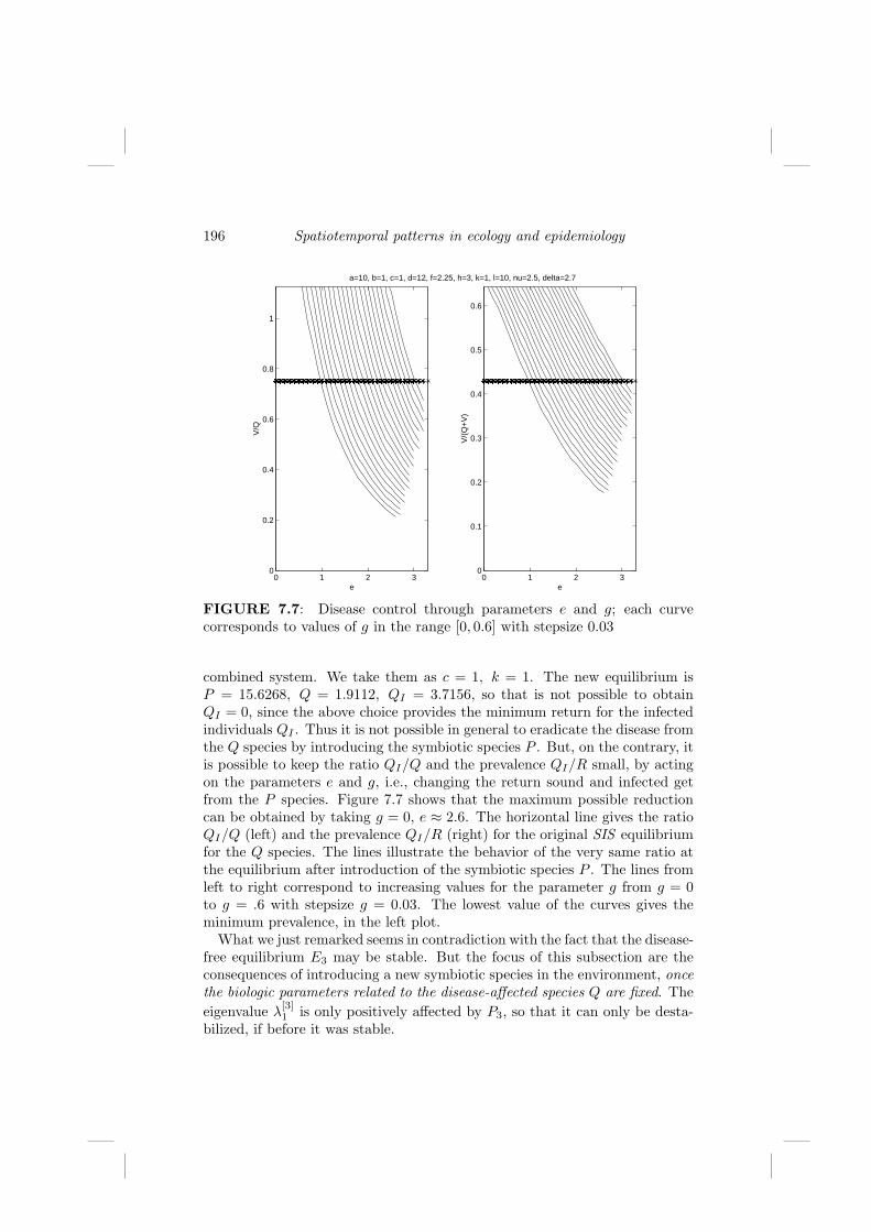
196 Spatiotemporal patterns in ecology and epidemiology
0 1 2 30
0.2
0.4
0.6
0.8
1
a=10, b=1, c=1, d=12, f=2.25, h=3, k=1, l=10, nu=2.5, delta=2.7
e
V/Q
0 1 2 30
0.1
0.2
0.3
0.4
0.5
0.6
e
V/(
Q+
V)
FIGURE 7.7: Disease control through parameters e and g; each curvecorresponds to values of g in the range [0, 0.6] with stepsize 0.03
combined system. We take them as c = 1, k = 1. The new equilibrium isP = 15.6268, Q = 1.9112, QI = 3.7156, so that is not possible to obtainQI = 0, since the above choice provides the minimum return for the infectedindividuals QI . Thus it is not possible in general to eradicate the disease fromthe Q species by introducing the symbiotic species P . But, on the contrary, itis possible to keep the ratio QI/Q and the prevalence QI/R small, by actingon the parameters e and g, i.e., changing the return sound and infected getfrom the P species. Figure 7.7 shows that the maximum possible reductioncan be obtained by taking g = 0, e ≈ 2.6. The horizontal line gives the ratioQI/Q (left) and the prevalence QI/R (right) for the original SIS equilibriumfor the Q species. The lines illustrate the behavior of the very same ratio atthe equilibrium after introduction of the symbiotic species P . The lines fromleft to right correspond to increasing values for the parameter g from g = 0to g = .6 with stepsize g = 0.03. The lowest value of the curves gives theminimum prevalence, in the left plot.
What we just remarked seems in contradiction with the fact that the disease-free equilibrium E3 may be stable. But the focus of this subsection are theconsequences of introducing a new symbiotic species in the environment, oncethe biologic parameters related to the disease-affected species Q are fixed. Theeigenvalue λ
[3]1 is only positively affected by P3, so that it can only be desta-
bilized, if before it was stable.