Spatio–Temporal Data Mining for Location–Based …gyozo/docs/thesis.pdfthe increasing...
210
Spatio–Temporal Data Mining for Location–Based Services Gy˝ oz˝ o Gid ´ ofalvi Ph.D. Thesis A thesis submitted to the Faculties of En- gineering, Science and Medicine at Aal- borg University, Denmark, in partial ful- fillment of the requirements for the Ph.D. degree in computer science. Copyright c 2007 by Gy ˝ oz˝ o Gid´ ofalvi
Transcript of Spatio–Temporal Data Mining for Location–Based …gyozo/docs/thesis.pdfthe increasing...
Spatio–Temporal Data Mining for Location–Based Services
Gyozo Gidofalvi
Ph.D. Thesis
A thesis submitted to the Faculties of En-gineering, Science and Medicine at Aal-borg University, Denmark, in partial ful-fillment of the requirements for the Ph.D.degree in computer science.
Copyright c© 2007 by Gyozo Gidofalvi


Abstract
Largely driven by advances in communication and information technology, such asthe increasing availability and accuracy of GPS technology and the miniaturization ofwireless communication devices, Location–Based Services (LBS) are continuouslygaining popularity. Innovative LBSes integrate knowledge about the users into theservice. Such knowledge can be derived by analyzing the location data of users. Suchdata contain two unique dimensions,spaceandtime, which need to be analyzed.
The objectives of this thesis are three–fold. First, to extend popular data miningmethods to the spatio–temporal domain. Second, to demonstrate the usefulnessof theextended methods and the derived knowledge in two promising LBS examples.Fi-nally, to eliminate privacy concerns in connection with spatio–temporal data miningby devising systems for privacy–preserving location data collection and mining.
To this extent, Chapter 2 presents a general methodology,pivoting, to extend apopular data mining method, namely rule mining, to the spatio–temporal domain. Byconsidering the characteristics of a number of real–world data sources,Chapter 2 alsoderives a taxonomy of spatio–temporal data, and demonstrates the usefulness of therules that the extended spatio–temporal rule mining method can discover. In Chapter4 the proposed spatio–temporal extension is applied to find long, sharable patternsin trajectories of moving objects. Empirical evaluations show that the extendedme-thod and its variants, using high–level SQL implementations, are effective tools foranalyzing trajectories of moving objects.
Real–world trajectory data about a large population of objects moving over ex-tended periods within a limited geographical space is difficult to obtain. To aid thedevelopment in spatio–temporal data management and data mining, Chapter 3 devel-ops a Spatio–Temporal ACTivity Simulator (ST–ACTS). ST–ACTS uses a number ofreal–world geo–statistical data sources and intuitive principles to effectively generaterealistic spatio–temporal activities of mobile users.
Chapter 5 proposes an LBS in the transportation domain, namely cab–sharing.To deliver an effective service, a unique spatio–temporal grouping algorithm is pre-sented and implemented as a sequence of SQL statements. Chapter 6 identifies ascalability bottleneck in the grouping algorithm. To eliminate the bottleneck, the
i

ii Abstract
chapter expresses the grouping algorithm as a continuous stream queryin a datastream management system, and then devises simple but effective spatio–temporalpartitioning methods for streams to parallelize the computation. Experimental resultsshow that parallelization through adaptive partitioning methods leads to speed–upsof orders of magnitude without significantly effecting the quality of the grouping.Spatio–temporal stream partitioning is expected to be an effective method to scalecomputation–intensive spatial queries and spatial analysis methods for streams.
Location–Based Advertising (LBA), the delivery ofrelevantcommercial infor-mation to mobile consumers, is considered to be one of the most promising businessopportunities amongst LBSes. To this extent, Chapter 7 describes an LBA frameworkand an LBA database that can be used for the management of mobile ads. Using asimulated but realistic mobile consumer population and a set of mobile ads, the LBAdatabase is used to estimate the capacity of the mobile advertising channel. The es-timates show that the channel capacity is extremely large, which is evidence for astrong business case, but it also necessitates adequate user controls.
When data about users is collected and analyzed, privacy naturally becomes aconcern. To eliminate the concerns, Chapter 8 first presents a grid–based frameworkin which location data is anonymized through spatio–temporal generalization, andthen proposes a system for collecting and mining anonymous location data. Exper-imental results show that the privacy–preserving data mining component discoverspatterns that, while probabilistic, are accurate enough to be useful for many LBSes.
To eliminate any uncertainty in the mining results, Chapter 9 proposes a systemfor collectingexacttrajectories of moving objects in a privacy–preserving manner. Inthe proposed system there are no trusted components and anonymization is performedby the clients in a P2P network via data cloaking and data swapping. Realistic sim-ulations show that under reasonable conditions and privacy/anonymity settings theproposed system is effective.

Acknowledgments
This thesis is the result of an industrial Ph.D. study, which is a unique mix of theoryand practice. This study would not have been possible without the support of thefollowing organizations: Geomatic ApS, Aalborg University, in particular theDe-partment of Computer Science, and the Danish Ministry of Science, Technology, andInnovation, which has supported the study under grant number 61480.I would like tothank these organizations for the unforgettable life experience and the priceless giftof a world–class education.
I believe that motivation plays a very significant role in a person’s education.Among the numerous people that provided me motivation, I would like to grate-fully acknowledge the help of Professors Sara Baase, Mahmoud Tarokh, RomanSwiniarski, and Charles Elkan. Most importantly, I would like to acknowledgemyPh.D. advisor, Torben Bach Pedersen, for all his motivation and insightsthroughoutmy graduate career. Apart from teaching me the principles of research and academicwriting, he has also introduced me to several new and exciting topics in the area ofspatio–temporal data management and analysis. Similarly, I would like to acknowl-edge Professor Tore Risch for filling a similar role during my stay–abroad study atUppsala University.
Furthermore, I would like to thank all my colleges in Geomatic, the members ofthe Database and Programming Technologies Group at Aalborg University, and themembers of the Uppsala Database Laboratory at Uppsala University for their helpand for providing a friendly and stimulating environment. In particular, I would liketo thank Martin K. Glarvig, Hans Ravnkjær Larsen, Lau Kingo Marcussen, JesperPersson, Esben Taudorf, Kasper Rugge, Susanne Caroc and Jesper Christiansen atGeomatic, Laurynas Speicys, Nerius Tradisauskas, Xuegang Huang and ChristianThomsen in the Database and Programming Technologies Group at Aalborg Univer-sity, and Erik Zeitler in the Uppsala Database Laboratory at Uppsala University.
Last, but not least, I would like to express my appreciation to my parents,Agnesand Zoltan, and my brother Gergely. I would not have been able to do it without theircontinuous support and motivation.
iii


Contents
Abstract i
Acknowledgments iii
Contents v
1 Introduction 1
2 Spatio–Temporal Rule Mining: Issues and Techniques 72.1 Introduction . . . . . . . . . . . . . . . . . . . . . . . . . . . . . . 72.2 Spatio–Temporal Data . . . . . . . . . . . . . . . . . . . . . . . . 10
2.2.1 Examples of ST Data Sets . . . . . . . . . . . . . . . . . . 102.2.2 A Taxonomy of ST Data . . . . . . . . . . . . . . . . . . . 11
2.3 Spatio–Temporal Baskets . . . . . . . . . . . . . . . . . . . . . . . 122.3.1 Mobile Entities with Static and Dynamic Attributes . . . . . 122.3.2 Immobile Entities with Static and Dynamic Attributes . . . 14
2.4 Issues in Spatio–Temporal Rule Mining . . . . . . . . . . . . . . . 172.5 Conclusions and Future Work . . . . . . . . . . . . . . . . . . . . . 18
3 ST–ACTS: A Spatio–Temporal Activity Simulator 193.1 Introduction . . . . . . . . . . . . . . . . . . . . . . . . . . . . . . 193.2 Related Work . . . . . . . . . . . . . . . . . . . . . . . . . . . . . 213.3 Problem Statement . . . . . . . . . . . . . . . . . . . . . . . . . . 223.4 Source Data . . . . . . . . . . . . . . . . . . . . . . . . . . . . . . 24
3.4.1 conzoomR© Demographic Data . . . . . . . . . . . . . . . . 243.4.2 mobidk
TMDaily Movement Data . . . . . . . . . . . . . . . 26
3.4.3 bizmarkTM
Business Data . . . . . . . . . . . . . . . . . . . 273.4.4 GallupPCR© Consumer Survey Data . . . . . . . . . . . . . 27
3.5 ST–ACTS: Spatio–Temporal ACTivity Simulator . . . . . . . . . . 273.5.1 Drawing Demographic Variables for Simpersons . . . . . . 283.5.2 Skewing Distributions Based on Correlations . . . . . . . . 28
v

vi CONTENTS
3.5.3 Assigning Simpersons to Work Places / Schools . . . . . . . 303.5.4 Daily Activity Probabilities . . . . . . . . . . . . . . . . . 313.5.5 Activity Simulation with Spatio–Temporal Constraints . . . 323.5.6 Discrete Event Simulation . . . . . . . . . . . . . . . . . . 34
3.6 Evaluation of the Simulation . . . . . . . . . . . . . . . . . . . . . 353.7 Conclusions and Future Work . . . . . . . . . . . . . . . . . . . . . 38
4 Mining Long, Sharable Patterns in Trajectories of Moving Objects 394.1 Introduction . . . . . . . . . . . . . . . . . . . . . . . . . . . . . . 394.2 Related Work . . . . . . . . . . . . . . . . . . . . . . . . . . . . . 414.3 Long, Sharable Patterns in Trajectories . . . . . . . . . . . . . . . . 43
4.3.1 From Trajectories to Transactions . . . . . . . . . . . . . . 434.3.2 Example Trajectory Database . . . . . . . . . . . . . . . . 464.3.3 Problem Statement . . . . . . . . . . . . . . . . . . . . . . 47
4.4 Naıve Approach to LSP Mining . . . . . . . . . . . . . . . . . . . 484.5 Projection–Based LSP Mining . . . . . . . . . . . . . . . . . . . . 49
4.5.1 STEP 1: Filtering of Infrequent Items . . . . . . . . . . . . 494.5.2 STEP 2: Filtering of Short Transactions . . . . . . . . . . . 504.5.3 STEP 3: Item–Conditional DB Projection . . . . . . . . . . 514.5.4 STEP 4: Discovery of the Single Most Frequent Closed Itemset 524.5.5 STEP 5: Deletion of Unnecessary Items . . . . . . . . . . . 534.5.6 Item–Projection Ordered by Increasingn–Support . . . . . 544.5.7 Alternating Pattern Discovery and Deletion . . . . . . . . . 554.5.8 LSP Mining Algorithm . . . . . . . . . . . . . . . . . . . . 57
4.6 Alternative Modelling of Trajectories and Mining of LSPs . . . . . 584.6.1 Macro Modelling of Trajectories and Mining of LSPs . . . . 594.6.2 Hybrid Modelling of Trajectories and Mining of LSPs . . . 60
4.7 Experimental Evaluation . . . . . . . . . . . . . . . . . . . . . . . 624.7.1 The INFATI Data Set . . . . . . . . . . . . . . . . . . . . . 624.7.2 The ST–ACTS Trajectory Data Set . . . . . . . . . . . . . . 634.7.3 The ST–ACTS Origin–Destination Data Set . . . . . . . . . 644.7.4 Sensitivity Experiments forMinSupp andMinLength Pa-
rameters . . . . . . . . . . . . . . . . . . . . . . . . . . . . 644.7.5 Scale–up Experiments for Various Input Data Sizes . . . . . 674.7.6 Global (Macro) Modelling and LSP Mining Experiments . . 694.7.7 Visualization of Patterns . . . . . . . . . . . . . . . . . . . 694.7.8 Summary of Experimental Results . . . . . . . . . . . . . . 71
4.8 Conclusions and Future Work . . . . . . . . . . . . . . . . . . . . . 71

CONTENTS vii
5 Cab–Sharing: An Effective, On–Demand Transportation Service 735.1 Introduction . . . . . . . . . . . . . . . . . . . . . . . . . . . . . . 735.2 Problem Statement . . . . . . . . . . . . . . . . . . . . . . . . . . 745.3 Cab–Sharing Service . . . . . . . . . . . . . . . . . . . . . . . . . 755.4 Grouping of Cab Requests . . . . . . . . . . . . . . . . . . . . . . 765.5 A Simple SQL Implementation . . . . . . . . . . . . . . . . . . . . 77
5.5.1 STEP 1: Calculating Fractional Extra Costs . . . . . . . . . 785.5.2 STEP 2: Calculating Amortized Costs . . . . . . . . . . . . 795.5.3 STEP 3: Selecting the Best Cab–Share . . . . . . . . . . . 795.5.4 STEP 4: Pruning the Search Space . . . . . . . . . . . . . . 805.5.5 Periodic, Iterative Scheduling of Cab Requests . . . . . . . 80
5.6 Experiments . . . . . . . . . . . . . . . . . . . . . . . . . . . . . . 805.7 Conclusions and Future Work . . . . . . . . . . . . . . . . . . . . . 83
6 Highly Scalable Trip Grouping for Large–Scale Collective Transporta-tion Systems 856.1 Introduction . . . . . . . . . . . . . . . . . . . . . . . . . . . . . . 866.2 Related Work . . . . . . . . . . . . . . . . . . . . . . . . . . . . . 876.3 Vehicle–Sharing . . . . . . . . . . . . . . . . . . . . . . . . . . . . 90
6.3.1 The Vehicle–Sharing Problem . . . . . . . . . . . . . . . . 906.3.2 Overview of the Cab–Sharing System . . . . . . . . . . . . 916.3.3 A Trip Grouping Algorithm . . . . . . . . . . . . . . . . . 916.3.4 Problems with Large–Scale CT Systems . . . . . . . . . . . 936.3.5 Ride–Sharing Application Requirements . . . . . . . . . . 956.3.6 Application of the TG Algorithm in an RSS . . . . . . . . . 95
6.4 Highly Scalable Trip Grouping . . . . . . . . . . . . . . . . . . . . 966.4.1 Processing of a Request Stream . . . . . . . . . . . . . . . 966.4.2 Parallel Stream Processing in SCSQ . . . . . . . . . . . . . 976.4.3 Spatial Partitioning Methods . . . . . . . . . . . . . . . . . 98
6.4.3.1 Baseline Queries . . . . . . . . . . . . . . . . . . 996.4.3.2 Static, Point Quad Partitioning . . . . . . . . . . 1006.4.3.3 Static, KD Partitioning . . . . . . . . . . . . . . 1016.4.3.4 Adaptive, Point Quad Partitioning . . . . . . . . . 1026.4.3.5 Adaptive, KD Partitioning . . . . . . . . . . . . . 103
6.5 Density–Based Spatial Stream Partitioning . . . . . . . . . . . . . . 1046.6 Experiments . . . . . . . . . . . . . . . . . . . . . . . . . . . . . . 105
6.6.1 Baseline Performance . . . . . . . . . . . . . . . . . . . . 1066.6.2 Absolute Performance of the Parallel TG Algorithms . . . . 1076.6.3 Relative Performance of the Parallel TG Algorithms . . . . 110
6.7 Conclusions and Future Work . . . . . . . . . . . . . . . . . . . . . 111

viii CONTENTS
7 Estimating the Capacity of the Location–Based Advertising Channel 1137.1 Introduction . . . . . . . . . . . . . . . . . . . . . . . . . . . . . . 1147.2 Related Work . . . . . . . . . . . . . . . . . . . . . . . . . . . . . 1157.3 Problem Statement . . . . . . . . . . . . . . . . . . . . . . . . . . 1167.4 Data . . . . . . . . . . . . . . . . . . . . . . . . . . . . . . . . . . 117
7.4.1 conzoomR© Demographic Data . . . . . . . . . . . . . . . . 1177.4.2 GallupPCR© Consumer Survey Data . . . . . . . . . . . . . 1187.4.3 bizmark
TMProducts and Services . . . . . . . . . . . . . . 119
7.4.4 Simulating Mobile Users with ST–ACTS . . . . . . . . . . 1207.5 Method . . . . . . . . . . . . . . . . . . . . . . . . . . . . . . . . 121
7.5.1 LBA Relational Database . . . . . . . . . . . . . . . . . . . 1217.5.2 Proximity Requirements on Mobile Ads . . . . . . . . . . . 1227.5.3 Interests Based on Demography . . . . . . . . . . . . . . . 1227.5.4 LBA – Implicit Interest Case . . . . . . . . . . . . . . . . . 1237.5.5 LBA – Explicit Interest Case . . . . . . . . . . . . . . . . . 1247.5.6 Uniqueness and User–Defined Quantitative Constraints on
Mobile Ads . . . . . . . . . . . . . . . . . . . . . . . . . . 1247.5.7 User–Defined ST Constraints on Mobile Ads . . . . . . . . 1247.5.8 Inferring Personal Interests and Relevance Based on Histori-
cal User–Behavior . . . . . . . . . . . . . . . . . . . . . . 1257.5.9 An Operational LBA Database . . . . . . . . . . . . . . . . 127
7.6 Proposal for a Revenue Model for LBA . . . . . . . . . . . . . . . 1277.7 Experiments and Results . . . . . . . . . . . . . . . . . . . . . . . 1287.8 Conclusions and Future Work . . . . . . . . . . . . . . . . . . . . . 131
8 Privacy–Preserving Data Mining on Moving Object Trajectories 1338.1 Introduction . . . . . . . . . . . . . . . . . . . . . . . . . . . . . . 1338.2 Spatio–Temporal Anonymization . . . . . . . . . . . . . . . . . . . 136
8.2.1 Practical “Cut–Enclose” Implementation . . . . . . . . . . 1388.2.2 Problems with Existing Methods . . . . . . . . . . . . . . . 139
8.3 A Grid–Based Solution . . . . . . . . . . . . . . . . . . . . . . . . 1408.3.1 Grid–Based Anonymization . . . . . . . . . . . . . . . . . 1408.3.2 System Architecture . . . . . . . . . . . . . . . . . . . . . 1428.3.3 Finding Dense Spatio–Temporal Areas . . . . . . . . . . . 144
8.4 Evaluation . . . . . . . . . . . . . . . . . . . . . . . . . . . . . . . 1468.5 Conclusions and Future Work . . . . . . . . . . . . . . . . . . . . . 149
9 Privacy–Preserving Trajectory Collection 1519.1 Introduction . . . . . . . . . . . . . . . . . . . . . . . . . . . . . . 1519.2 Related Work . . . . . . . . . . . . . . . . . . . . . . . . . . . . . 1539.3 Preliminaries . . . . . . . . . . . . . . . . . . . . . . . . . . . . . 154

CONTENTS ix
9.4 Solution . . . . . . . . . . . . . . . . . . . . . . . . . . . . . . . . 1569.4.1 System Architecture . . . . . . . . . . . . . . . . . . . . . 1579.4.2 Client Registration . . . . . . . . . . . . . . . . . . . . . . 1599.4.3 Trajectory Sampling and Anonymization . . . . . . . . . . 1609.4.4 Trajectory Exchange . . . . . . . . . . . . . . . . . . . . . 1649.4.5 Data Reporting . . . . . . . . . . . . . . . . . . . . . . . . 1689.4.6 Data Summarization . . . . . . . . . . . . . . . . . . . . . 1699.4.7 Neighborhood Detection in P2P Networks . . . . . . . . . . 171
9.5 Discussion . . . . . . . . . . . . . . . . . . . . . . . . . . . . . . . 1719.5.1 Privacy at the Server . . . . . . . . . . . . . . . . . . . . . 1719.5.2 Privacy at Clients . . . . . . . . . . . . . . . . . . . . . . . 1729.5.3 Privacy in the Air . . . . . . . . . . . . . . . . . . . . . . . 172
9.6 Empirical Evaluation . . . . . . . . . . . . . . . . . . . . . . . . . 1729.7 Conclusions and Future Work . . . . . . . . . . . . . . . . . . . . . 179
10 Summary 18110.1 Summary of Conclusions . . . . . . . . . . . . . . . . . . . . . . . 18110.2 Summary of Research Directions . . . . . . . . . . . . . . . . . . . 183
Bibliography 187
Summary in Danish 197


Chapter 1
Introduction
Recent advances in communication and information technology, such as the increas-ing accuracy of GPS technology and the miniaturization of wireless communicationdevices pave the road for Location–Based Services (LBS). To achieve high qualityfor such services, data mining techniques are used for the analysis of thehuge amountof data collected from location–aware mobile devices. The objectives of thisthesisare three–fold. First, since the two most important attributes of the data collectedarelocationandtime, the thesis investigates general methods for extending existingdata mining methods to the spatio–temporal domain. Second, using two promisingLBSes, the thesis demonstrates the usefulness of the knowledge that can be extractedby the spatio–temporal data mining methods. Finally, since privacy is a major con-cern to users of LBSes, the thesis considers location privacy in connection with col-lection and data mining of location traces (trajectories) of users.
In the thesis the following setting and broad definitions are assumed. Mobileusers carry location–enabled mobile terminals (PDA, mobile phone, etc). By location–enabled it is meant that applications running on the mobile terminal have the abilityto get the current, historical, or potentially even future locations of the mobile user.Localization of the mobile terminals can be achieved through a wide variety of po-sitioning technologies, including but not limited to, cellular network based position-ing, GPS based positioning, geo–referenced sensor based positioning, or even geo–referenced user entry. Mobile users access LBSes through their mobileterminals.An LBS is a service that has one or more of the following characteristics. AnLBSis either explicitly or implicitly requested by the users via the mobile terminal. AnLBS delivers its service selectively based on the context of the mobile user. Thereare many aspects of user–context, however in this thesis the following context aspectsare considered: the current, historical and future locations of the user, any possibleuser–patterns in the user location data, and common patterns in the location dataof agroup of users.
1

2 Introduction
Data mining, the process of finding, e.g., associations, or in general patterns,within large amounts of data, often stored in relational databases, has beenappliedsuccessfully in the past to increase business revenue. More recently,data mining hasbeen suggested to be useful to derive context for user–friendly LBSes. A large part ofthis context for many LBSes can be described by general patterns in user activities.One type of user activity iswhereandwhenusers were in the past. Data miningmethods for such activities have to consider two additional dimensions, namelythespatial, thetemporalor jointly thespatio–temporaldimension, and are referred to asspatio–temporal data mining methods. Due to the unique nature of the two additionaldimensions, i.e., the cardinality of the dimensions are potentially extremely large,and the temporal dimension is cyclic for some types of applications, mining spatio–temporal patterns poses additional challenges. To address these challenges, Chapter2 presents a general methodology,pivoting, to extend heavily researched rule miningmethods, in particular association rule mining. By considering the characteristics ofa number of real–world data sources, Chapter 2 also derives a taxonomyof spatio–temporal data, and demonstrates the usefulness of the rules that the extended spatio–temporal rule mining method can mine.
Chapter 4 uses pivoting to extend a projection–based frequent itemset miningmethod to discover spatio–temporal sequential patterns, i.e., frequent routes, in GPStraces. The extended method, through (either region–based or road network based)spatio–temporal generalization, first preprocesses the GPS traces to obtain spatio–temporal itemsets. Then, a variant of a database projection based closed frequentitemset mining method prunes the search space by making use of the minimumlength and sharable requirements and avoids the generation of the exponential num-ber of sub–routes of long routes. Considering alternative modelling options for tra-jectories leads to the development of two effective variants of the method. SQL–based implementations are described, and extensive experiments on both real–life-and large–scale synthetic data show the effectiveness of the method and itsvariants.
Simulation is widely accepted in database research as a low–cost method to pro-vide synthetic data for designing and testing novel data types and access methods.This is even more so the case for trajectory data, where the availability of real–worlddata about a large population of moving objects is limited. Prior research produceda number of moving object simulators that model the physical aspects of mobilityto various degrees, but fail to adequately address the importantsocial and geo–demographicalaspects of mobility. Modelling the latter aspects gives rise to uniquespatio–temporal data distributions with regularities. Hence, to aid the development inspatio–temporal data management and data mining, Chapter 3 develops ST–ACTS, aSpatio–Temporal ACTivity Simulator. ST–ACTS uses a number of real–worldgeo–statistical data sources and intuitive principles to generate realistic spatio–temporalactivities of mobile users. ST–ACTS considers that (1) objects (representing mobile
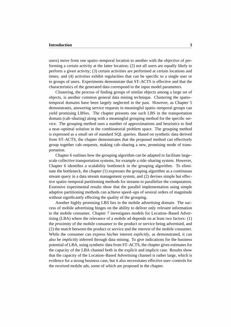
Introduction 3
users) move from one spatio–temporal location to another with the objective of per-forming a certain activity at the latter location; (2) not all users are equally likely toperform a given activity; (3) certain activities are performed at certainlocations andtimes; and (4) activities exhibit regularities that can be specific to a single user orto groups of users. Experiments demonstrate that ST–ACTS is effective and that thecharacteristics of the generated data correspond to the input model parameters.
Clustering, the process of finding groups of similar objects among a large set ofobjects, is another common general data mining technique. Clustering the spatio–temporal domains have been largely neglected in the past. However, as Chapter 5demonstrates, answering service requests in meaningful spatio–temporalgroups canyield promising LBSes. The chapter presents one such LBS in the transportationdomain (cab–sharing) along with a meaningful grouping method for the specific ser-vice. The grouping method uses a number of approximations and heuristics tofinda near–optimal solution in the combinatorial problem space. The grouping methodis expressed as a small set of standard SQL queries. Based on syntheticdata derivedfrom ST–ACTS, the chapter demonstrates that the proposed method can effectivelygroup together cab–requests, making cab–sharing a new, promising modeof trans-portation.
Chapter 6 outlines how the grouping algorithm can be adapted to facilitate large–scale collective transportation systems, for example a ride–sharing system.However,Chapter 6 identifies a scalability bottleneck in the grouping algorithm. To elimi-nate the bottleneck, the chapter (1) expresses the grouping algorithm as acontinuousstream query in a data stream management system, and (2) devises simple buteffec-tive spatio–temporal partitioning methods for streams to parallelize the computation.Extensive experimental results show that the parallel implementation using simpleadaptive partitioning methods can achieve speed–ups of several orders of magnitudewithout significantly effecting the quality of the grouping.
Another highly promising LBS lies in the mobile advertising domain. The suc-cess of mobile advertising hinges on the ability to deliver onlyrelevantinformationto the mobile consumer. Chapter 7 investigates models for Location–Based Adver-tising (LBA) where the relevance of a mobile ad depends on at least two factors: (1)theproximityof the mobile consumer to the product or service being advertised, and(2) thematchbetween the product or service and theinterestof the mobile consumer.While the consumer can express his/her interestexplicitly, as demonstrated, it canalso beimplicitly inferred through data mining. To give indications for the businesspotential of LBA, using synthetic data from ST–ACTS, the chapter gives estimates forthe capacity of the LBA channel both in the explicit and implicit case. Results showthat the capacity of the Location–Based Advertising channel is rather large, which isevidence for a strong business case, but it also necessitates effective user–controls forthe received mobile ads, some of which are proposed in the chapter.
4 Introduction
To receive LBSes, users have to be willing to disclose their current, historical,or future locations. Such a disclosure naturally raises concerns among the usersabout potentially being tracked and followed. Hence, to assure user acceptance ofLBSes, the privacy of users is of great importance. To this extent, Chapters 8 and 9address location privacy concerns in connection with data mining of user locations.More specifically, Chapter 8 proposes a privacy–preserving locationdata collectionand mining system. The system uses a general framework that allows user locationdata to be anonymized through spatio–temporal generalization, thus preserving pri-vacy. The data mining component of the system mines anonymized location dataand derives probabilistic spatio–temporal patterns. A privacy–preserving method isproposed for the core data mining task offinding dense spatio–temporal regions. Anextensive set of experiments evaluate the method, comparing it to its non–privacy–preserving equivalent. The experiments show that the framework allows most pat-terns to be found, even when privacy is preserved.
The anonymization process proposed in Chapter 8 introduces some uncertainty inthe patterns. To eliminate this uncertainty in patterns, Chapter 9 first adopts and com-bines existing privacy definitions to derive privacy definitions of various strengths forlocation data. Then the chapter presents a complete system for the privacy–preservingcollection ofexacttrajectories. The system is composed of an untrusted server andclients communicating in a P2P network. Location data is anonymized in the systemusing data cloaking and data swapping techniques. Experiments on simulated but re-alistic movement data indicate that the proposed system is effective under reasonableconditions and privacy / anonymity settings.
The contents of this thesis are based on the contents of papers that have eitherbeen published, are to appear, or are under consideration for publication.
Since Chapters 2 to 9 are based on individual publications, they are self containedand can be read in isolation. Since some of these chapters are closely related, this en-tails a certain amount of overlap. In particular, some of the methods and the basedata used in the data generator, ST–ACTS, in Chapter 3, are also used in the estima-tions in Chapter 7. Hence, there is a strong correspondence between Sections 3.4 and3.5.4, and Sections 7.5.3 and 7.4, respectively. Furthermore, since ST–ACTS is usedto generate synthetic data for experiments in most of the papers and is referencedextensively throughout the chapters, it is placed early in the thesis. Similarly, sinceChapter 6 provides a scalable implementation of the algorithm presented in Chapter5, the motivation in Section 5.1, the problem definition in Section 5.2, the servicedescription in Section 5.3, and the description of the basic algorithm in Section 5.4closely correspond to Sections 6.1, 6.3.1, 6.3.2, and 6.3.3, respectively.Finally, sinceboth Chapters 8 and 9 consider location privacy in connection with data miningoftrajectories, the motivations and review of related work in Section 8.1 are similartothat presented in Sections 9.1 and 9.2.

Introduction 5
The papers that the thesis is based on are listed below. Papers 3 and 6 areextendedjournal versions of the conference papers 9 and 10, respectively.Chapters 2 to 9 arebased on papers 1 to 8, respectively.
1. G. Gidofalvi and T. B. Pedersen. Spatio–Temporal Rule Mining: Issues andTechniques. InProc. of the 7th International Conference on Data Warehousingand Knowledge Discovery, DaWaK, volume 3589 of Lecture Notes in computerScience, pp. 275–284, Springer, 2005.
2. G. Gidofalvi and T. B. Pedersen. ST–ACTS: A Spatio–Temporal Activity Sim-ulator. In Proc. of the 14th ACM International Symposium on GeographicInformation Systems, ACM–GIS, pp. 155–162, ACM, 2006.
3. G. Gidofalvi and T. B. Pedersen. Mining Long, Sharable Patterns in Trajecto-ries of Moving Objects. To appear inGeoinformatica, 35 pages, 2008.
4. G. Gidofalvi and T. B. Pedersen. Cab–Sharing: An Effective, Door–To–Door,On–Demand Transportation Service. InProc. of the 6th European Congressand Exhibition on Intelligent Transport Systems and Services, ITS, 2007.
5. G. Gidofalvi, T. B. Pedersen, T. Risch, and E. Zeitler. Highly Scalable TripGrouping for Large–Scale Collective Transportation Systems. To appear inProc. of the 11th International Conference on Extending Database Technology,EDBT, 12 pages, 2008.
6. G. Gidofalvi, H. R. Larsen, and T. B. Pedersen. Estimating the Capacity of theLocation–Based Advertising Channel. To appear inInternational Journal ofMobile Communications, IJMC, 18 pages, Inderscience Publishers, 2008.
7. G. Gidofalvi, X. Huang, and T. B. Pedersen. Privacy–Preserving Data Miningon Moving Object Trajectories. InProc. of the 8th International Conferenceon Mobile Data Management, MDM, 2007.
8. G. Gidofalvi, X. Huang, and T. B. Pedersen. Privacy–Preserving TrajectoryCollection. Submitted tothe 2008 ACM SIGMOD International Conferenceon Management of Data, SIGMOD, 12 pages, 2008.
9. G. Gidofalvi and T. B. Pedersen. Mining Long, Sharable Patterns in Trajec-tories of Moving Objects. InProc. of the 3rd Workshop on Spatio–TemporalDatabase Management, STDBM, volume 174 of Online Proceedings of CEUR–WS, pp. 49–58, CEUR–WS, 2006.
10. G. Gidofalvi, H. R. Larsen, and T. B. Pedersen. Estimating the Capacity ofthe Location–Based Advertising Channel. InProc. of the 2007 InternationalConference on Mobile Business, ICMB, pp. 2, IEEE Computer Society, 2007.


Chapter 2
Spatio–Temporal Rule Mining:Issues and Techniques
Recent advances in communication and information technology, such as the increas-ing accuracy of GPS technology and the miniaturization of wireless communicationdevices pave the road for Location–Based Services (LBS). To achieve high qualityfor such services, spatio–temporal data mining techniques are needed. This paper de-scribes experiences with spatio–temporal rule mining in a Danish data mining com-pany. First, a number of real world spatio–temporal data sets are described, leading toa taxonomy of spatio–temporal data. Second, the paper describes a general method-ology that transforms the spatio–temporal rule mining task to the traditional marketbasket analysis task and applies it to the described data sets, enabling traditional as-sociation rule mining methods to discover spatio–temporal rules for LBS. Finally,unique issues in spatio–temporal rule mining are identified and discussed.
2.1 Introduction
Several trends in hardware technologies such as display devices and wireless com-munication combine to enable the deployment of mobile, Location–Based Services(LBS). Perhaps most importantly, global positioning systems (GPS) are becomingincreasingly available and accurate. In the coming years, we will witness very largequantities of wirelessly Internet–worked objects that are location–enabledand capa-ble of movement to varying degrees. These objects include consumers using GPRSand GPS enabled mobile–phone terminals and personal digital assistants, tourists
7

8 Spatio–Temporal Rule Mining: Issues and Techniques
carrying on–line and position–aware cameras and wrist watches, vehicles with com-puting and navigation equipment, etc.
These developments pave the way to a range of qualitatively new types of Internet–based services [56]. These types of services, which either make little sense or are oflimited interest in the context of fixed–location, desktop computing, include: trafficcoordination and management, way–finding, location–aware advertising, integratedinformation services, e.g., tourist services.
A single generic scenario may be envisioned for these location–based services.Moving service users disclose their positional information to services, which use thisand other information to provide specific functionality. To customize the interactionsbetween the services and users, data mining techniques can be applied to discoverinteresting knowledge about the behavior of users. For example, groups of users canbe identified exhibiting similar behavior. These groups can be characterized basedon various attributes of the group members or the requested services. Sequences ofservice requests can also be analyzed to discover regularities in such sequences. Laterthese regularities can be exploited to make intelligent predictions about user’s futurebehavior given the requests the user made in the past. In addition, this knowledge canalso be used for delayed modification of the services, and for longer–term strategicdecision making [57].
An intuitively easy to understand representation of this knowledge is in termsof rules. A rule is an implication of the formA ⇒ B, whereA andB are setsof attributes. The idea of mining association rules and the subproblem of miningfrequent itemset was introduced by Agrawal et al. for the analysis of market basketdata [1]. Informally, the task of mining frequent itemsets can be defined as findingall sets of items that co–occur in user purchases more than a user–defined number oftimes. The number of times items in an itemset co–occur in user purchases is definedto be thesupportof the itemset. Once the set of high–support, so calledfrequentitemsets have been identified, the task of mining association rules can be defined asfinding disjoint subsetsA andB of each frequent itemset such that the conditionalprobability of items inB given the items inA is higher than a user–defined threshold.The conditional probability ofB givenA is referred to as theconfidenceof the ruleA ⇒ B. Given that coffee and cream are frequently purchased together, ahigh–confidence rule might be that “60% of the people who buy coffee also buycream.”Association rule mining is an active research area. For a detailed review thereader isreferred to [40].
Spatio–temporal (ST) rules can be eitherexplicit or implicit. Explicit ST ruleshave a pronounced ST component. Implicit ST rules encode dependencies betweenentities that are defined by spatial (north–of, within, close–to,. . . ) and/ortemporal(after, before, during,. . . ) predicates. An example of an explicit ST rule is: “Busi-nessmen drink coffee at noon in the pedestrian street district.” An exampleof an

2.1 Introduction 9
implicit ST rule is: “Middle–aged single men often co–occur in space and time withyounger women.” This paper describes experiences with ST rule mining in the Dan-ish spatial data mining company, Geomatic.
The task of finding ST rules is challenging because of the high cardinality ofthetwo added dimensions: space and time. Additionally, straight–forward application ofassociation rule mining methods cannot always extract all the interesting knowledgein ST data. For example, consider the previous implicit ST rule example, whichextracts knowledge about entities (people) with different attributes (gender, age) thatinteract in space and time. Such interaction will not be detected when associationrule mining is applied in straight–forward manner. This creates a need to explore thespecial properties of ST data in relation to rule mining, which is the focus of thispaper.
The contributions of the paper are as follows. First, a number of real world STdata sets are described, and a taxonomy for ST data is derived. Second, havingthe taxonomy, the described data sets, and the desirable LBSes in mind, a generalmethodology is devised that projects the ST rule mining task to traditional marketbasket analysis. The proposed method can in many cases efficiently eliminatetheabove mentioned explosion of the search space, and allows for the discovery of bothimplicit and explicit ST rules. Third, the projection method is applied to a numberof different type of ST data such that traditional association rule mining methods areable to find ST rules which are useful for LBSes. Fourth, as a natural extension to theproposed method, spatio–temporally restricted mining is described, which in somecases allows for further quantitative and qualitative mining improvements. Finally,a number of issues in ST rule mining are identified, which point to possible futureresearch directions.
Despite the abundance of ST data, the number of algorithms that mine such datais small. Since the pioneering work of [2], association rule mining methods wereextended to the spatial [21, 22, 48, 63], and later to the temporal dimension [67].Other than in [70, 95], there has been no attempts to handle the combination of thetwo dimensions. In [95] an efficient depth–first search style algorithm is given todiscover ST sequential patterns in weather data. The method does not fullyexplorethe spatial dimension as no spatial component is present in the rules, and nogeneralspatial predicate defines the dependencies between the entities. In [70],a bottom–up, level–wise, and a faster top–down mining algorithm is presented to discover STperiodic patterns in ST trajectories. While the technique can naturally be appliedto discover ST event sequences, the patterns found are only within a single eventsequence.
The remainder of the paper is organized as follows. Section 2.2 introducesa num-ber of real world ST data sets, along with a taxonomy of ST data. In Section 2.3, ageneral methodology is introduced that projects the ST rule mining task to the tradi-

10 Spatio–Temporal Rule Mining: Issues and Techniques
tional market basket analysis or frequent itemset mining task. The proposed problemprojection method is also applied to the example data sets such that traditional associ-ation rule mining methods are able to discover ST rules for LBSes. Finally, Sections2.4 and 2.5 identify unique issues in ST rule mining, conclude, and point to futurework.
2.2 Spatio–Temporal Data
Data is obtained by measuring some attributes of an entity/phenomena. When theseattributes depend on the place and time the measurements are taken, the data is referto as ST data. Hence such ST measurements not only include the measured attributevalues about the entity or phenomena, but also two special attribute values:a locationvalue,wherethe measurement was taken, and a time value,whenthe measurementwas taken. Disregarding these attributes, the non–ST rule “Businessmen drink cof-fee” would result in annoying advertisements sent to businessmen who arein themiddle of an important meeting.
2.2.1 Examples of ST Data Sets
The first ST data set comes from the “Space, Time, and Man” (STM) project [86]—a multi–disciplinary project at Aalborg University. In the STM project activities ofthousands of individuals are continuously registered through GPS–enabled mobilephones, referred to as mobile terminals. These mobile terminals, integrated withvarious GIS services, are used to determine close–by services such asshops. Basedon this information in certain time intervals the individual is prompted to select fromthe set of available services, which s/he currently might be using. Upon thisselection,answers to subsequent questions can provide a more detailed information about thenature of the used service. Some of the attributes collected include: location and timeattributes, demographic user attributes, and attributes about the services used. Thisdata set will be referred to as STM in the following.
The second ST data set is a result of a project carried out by the Greater Copen-hagen Development Council (Hovedstadens Udviklings Rad (HUR)). The HUR pro-ject involves a number of city busses each equipped with a GPS receiver,a laptop,and infrared sensors for counting the passengers getting on and off at each bus stop.While the busses are running, their GPS positions are continuously sampled toobtaindetailed location information. The next big project of HUR will be to employ chipcards as payment for the travel. Each passenger must have an individual chip cardthat is read when getting on and off the bus. In this way an individual payment de-pendent on the person and the length of the travel can be obtained. The data recordedfrom the chip cards can provide valuable passenger information. When analyzed, the

2.2 Spatio–Temporal Data 11
data can reveal general travel patterns that can be used for suggesting new and betterbus routes. The chip cards also reveal individual travel patterns which can be usedto provide a customized LBS that suggests which bus to take, taking capacitiesandcorrect delays into account. In the following, the data sets from the first and secondprojects of HUR will be referred to as HUR1 and HUR2, respectively.
The third ST data set is the publicly available INFATI data set [53], which comesfrom the intelligent speed adaptation (INtelligent FArtTIlpasning (INFATI)) projectconducted by the Traffic Research Group at Aalborg University. Thisdata set recordscars moving around in the road network of Aalborg, Denmark over a period of sev-eral months. During this period, periodically the location and speeds of the cars aresampled and matched to corresponding speed limits. This data set is interesting,as itcaptures the movement of private cars on a day–to–day basis, i.e., the dailyactivitypatterns of the drivers. Additional information about the project can be found in [58].This data set will be referred to as INFATI in the following.
Finally, the last example data set comes from the Danish Meteorology Institute(DMI) and records at fixed time intervals atmospheric measurements like tempera-ture, humidity, and pressure for Denmark for 5 km grid cells. This data setis uniquein that unlike the other data sets it does not capture ST characteristics of moving ob-jects, but nonetheless is ST. This data set will be referred to as DMI in the following.
2.2.2 A Taxonomy of ST Data
Data mining in the ST domain is yet largely unexplored. There does not even existany generally accepted taxonomy of ST data. To analyze such data it is important toestablish a taxonomy.
Perhaps the most important criterion for this categorization is whether the mea-sured entities aremobileor immobile. The ST data in the DMI data set is immobilein the sense that the temperature or the amount of sunshine does not move from onelocation to the other, but rather, as a continuous phenomenon, changes itsattributevalue over time at a given location. On the other hand, the observed entities intheother four data sets are rather mobile.
Another important criterion for categorization is whether the attribute values ofthe measured entities arestatic or dynamic. There are many examples of static at-tributes values but perhaps one that all entities possess is a unique identifier. Dy-namic attributes values change over time. This change can be slow and gradual, likein the case of the age of an observed entity, or swift and abrupt, like in the case ofan activity performed by the observed entity, which starts at a particular time and lastfor a well–specified time interval only.

12 Spatio–Temporal Rule Mining: Issues and Techniques
2.3 Spatio–Temporal Baskets
Following the methodology of market basket analysis, to extract ST rules for a givendata set, one needs to define STitemsandbaskets. This task is important, since anypossible knowledge that one can extract using association rule mining methods willbe about the possible dependencies of the items within the baskets.
2.3.1 Mobile Entities with Static and Dynamic Attributes
Consider the STM data; it is mobile in nature and has several static and dynamicattributes. Base data contains the identity and some demographic attributes of theuser, and the activity performed by user at a particular location and time. Furtherattributes of the locations where the activity is performed are also available. Byapplying association rule mining on this base data one can find possible dependenciesbetween the activities of the users, the demographics of the users, the characteristicsof the locations there the activities are performed, and the location and time of theactivities. Since the location and time attributes are items in the baskets one may findStrøget,noon,businessman,cafe as a frequent itemset and from it the associationruleStrøget,noon,businessman⇒ cafe. Strøget being a famous pedestrian streetdistrict in central Copenhagen in Denmark, this rule clearly has both a spatial andtemporal component and can be used to advertise special deals of a cafe shop onStrøget to businessmen who are in the area around noon.
In the INFATI data set, a record in the base data contains a location, a time, adriver identifier, and the current speed of the car along with the maximum allowedspeed at the particular location. The possible knowledge one can discover by apply-ing association rule mining on the base data is where and when drivers or a particulardriver occur(s) and/or speed(s) frequently. However, one may in asense pivot this ta-ble of base data records such that each new row represents an ST region and recordsthe car identifiers that happen to be in that region. Applying association rulemin-ing on these ST baskets one may find which cars co–occur frequently in space andtime. Such knowledge can be used to aid intelligent rideshare services. It can also bevaluable information for constructing traffic flow models and for discovering travelpatterns. While the possible knowledge discovered may be valuable for certain appli-cations, the extracted rules are not clearly ST, i.e.: there is noexplicit ST componentin them. In fact the same set of cars may frequently co–occur at severalST regionswhich may be scattered in space and time. Nonetheless, it can be argued thatsincethe “co–occurrence” between the items in the ST baskets is actually an ST predicatein itself, the extracted rules areimplicitly ST.
An alternative to this approach might be to restrict the mining of the ST basketsto larger ST regions. While this may seem useless at first, since the baskets them-selves already define more fine–grained ST regions, it has several advantages. First,

2.3 Spatio–Temporal Baskets 13
Location Time CarID
1 07:30 A
1 07:30 B
2 07:31 A
2 07:31 B
2 07:31 C
3 07:32 A
3 07:32 C
3 16:20 A
3 16:20 B
2 16:21 A
2 16:21 B
1 16:22 A
1 16:22 B
Location Time CarIDs
1 07:30 A,B
2 07:31 A,B,C
3 07:32 A,C
3 16:20 A,B
2 16:21 A.B
1 16:22 A,B
Base Data Records from INFATI
Spatio-temporal Baskets
Pivoting
Figure 2.1: Process of Pivoting to Obtain ST Baskets from INFATI Base Data.
it allows the attachment of an explicit ST component to each extracted rule. Second,it enhances the quality of the extracted rules. Finally, it significantly speedsup themining process, as no two itemsets from different regions are combined andtriedas a candidate. Figure 2.1 shows the process of pivoting of some example recordsabstracted from the INFATI data set. Figure 2.2 shows the process and results ofspatio–temporally restricted and unrestricted mining of the ST baskets. In this ex-ample the shown frequent itemsets are based on an absolute minimum support of 2in both cases, however in the restricted case specifying a relative minimum supportwould yield more meaningful results. Naturally the adjective “relative” refers to thenumber of baskets in each of the ST regions. Figure 2.2 also shows the above men-tioned qualitative differences in the result obtained from spatio–temporally restrictedvs. unrestricted mining. While the frequent co–occurrence of cars A and B, andcars A and C are detected by unrestricted mining, the information that cars A andB are approximately equally likely to co–occur in area A1 in the morning as in theafternoon, and that cars A and C only co–occur in area A1 in the morning ismissed.
Similar pivoting techniques based on other attributes can also reveal interestinginformation. Consider the data set in HUR2 and the task of finding frequentlytrav-elled routes originating from a given ST region. In the HUR2 data set a record isgenerated every time a user starts and finishes using a transportation service. Thisrecord contains the identifier of the user, the transportation line used, andthe locationand time of the usage. For simplicity assume that a trip is defined to last at most 2hours. As a first step of the mining, one can retrieve all the records that fall withinthe ST region of the origin. Following, one can retrieve all the records within2 hoursof the users that belonged to the first set. By pivoting on the user–identifiers, one canderive ST baskets that contain locations where the user generated a record by making

14 Spatio–Temporal Rule Mining: Issues and Techniques
Location Time CarIDs
1 07:30 A,B
2 07:31 A,B,C
3 07:32 A,C
3 16:20 A,B
2 16:21 A.B
1 16:22 A,B
Spatio-temporal region 1:Area = A1 Period = 07:30-07:40
Spatio-temporal region 2:Area = A1 Period = 16:20-16:30
Spatio-temporal Baskets
Spatio-temporallyUnrestricted Mining
Spatio-temporallyRestricted Mining
Itemset Support
A 6
B 5
C 2
A,B 5
A,C 2
Area Period Itemset Support
A1 7:30-7:40 A 3
A1 7:30-7:40 B 2
A1 7:30-7:40 C 2
A1 7:30-7:40 A,B 2
A1 7:30-7:40 A,C 2
A1 16:20-16:30 A 3
A1 16:20-16:30 B 3
A1 16:20-16:30 A,B 3
Figure 2.2: Process and Results of Spatio–Temporally Restricted vs. UnrestrictedMining of ST Baskets.
use of a transportation service. Applying association rule mining to the so–derivedST baskets one may find frequently travelled routes originating from a specific STregion. The pivoting process for obtaining such ST baskets and the results of miningsuch baskets is illustrated in a simple example in the light bordered box of Figure2.3. Naturally, the frequent itemset mining is only applied to the ”Unique Locations”column of the ST baskets. As before the minimum support is set to 2. Consideringthe spatial relation between the locations one might consider altering the bus routesto better meet customer needs. For example, if locations A and C are close by on theroad network, but no bus line exists with a suitable schedule between A and C, thenin light of the evidence, i.e., support of A,B,C is 2, such a line can be added.Notethat while the discovered frequent location sets do not encode any temporal relationbetween the locations, one can achieve this by simply placing ST regions into theSTbaskets as items. The pivoting process and the results of mining are shown inthedark bordered box of Figure 2.3. The discovered ST itemsets can help in adjustingtimetables of busses to best meet customer needs.
2.3.2 Immobile Entities with Static and Dynamic Attributes
So far the examples considered data sets that are mobile and have either static, dy-namic, or both types of attribute values. Now consider an immobile ST data withmostly dynamic attribute values, as the DMI data set. The base data can be viewed astransactions in a relational table with a timestamp, a location identifier and some at-mospheric measurements like temperature, humidity, and pressure. Considering the
2.3 Spatio–Temporal Baskets 15
Base Data Records from HUR2
User Location Time Line ON/OFF
X A 08:00 7 ON
X B 08:15 7 OFF
X B 08:20 14 ON
X C 08:25 14 OFF
Y A 08:00 7 ON
Y B 08:15 7 OFF
Y D 08:18 18 ON
Y E 08:25 18 OFF
Z A 08:00 7 ON
Z B 08:15 7 OFF
Z B 08:20 14 ON
Z C 08:25 14 OFF
Pivoting
User Locations Unique Locations
X A,B,B,C A,B,C
Y A,B,D,E A,B,D,E
Z A,B,B,C A,B,C
Spatio-temporal Baskets
Frequent ItemsetMining
Itemset Support
A 3
B 3
C 2
A,B 3
A,C 2
A,B,C 2
Pivoting
User Spatio-temporal Regions
X A_0800, B_0815, B_0820, C_0825
Y A_0800, B_0815, D_0818, E_0825
Z A_0800, B_0815, B_0820, C_0825
Spatio-temporal Baskets
FrequentItemsetMining
Itemset Support
A_0800 3
B_0815 3
C_0825 3
A_0800,B_0815 3
A_0800,C_0825 2
A_0800,B_0815,C_0825 2
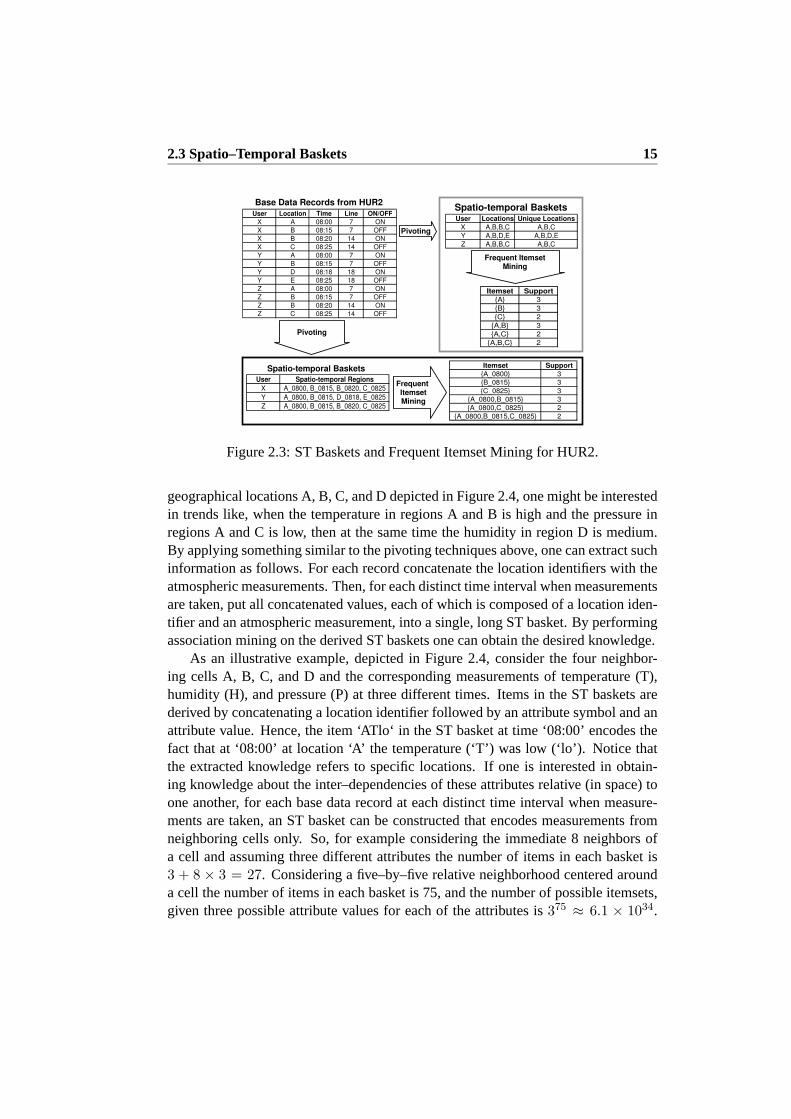
Figure 2.3: ST Baskets and Frequent Itemset Mining for HUR2.
geographical locations A, B, C, and D depicted in Figure 2.4, one might be interestedin trends like, when the temperature in regions A and B is high and the pressure inregions A and C is low, then at the same time the humidity in region D is medium.By applying something similar to the pivoting techniques above, one can extract suchinformation as follows. For each record concatenate the location identifierswith theatmospheric measurements. Then, for each distinct time interval when measurementsare taken, put all concatenated values, each of which is composed of a location iden-tifier and an atmospheric measurement, into a single, long ST basket. By performingassociation mining on the derived ST baskets one can obtain the desired knowledge.
As an illustrative example, depicted in Figure 2.4, consider the four neighbor-ing cells A, B, C, and D and the corresponding measurements of temperature(T),humidity (H), and pressure (P) at three different times. Items in the ST baskets arederived by concatenating a location identifier followed by an attribute symboland anattribute value. Hence, the item ‘ATlo‘ in the ST basket at time ‘08:00’ encodes thefact that at ‘08:00’ at location ‘A’ the temperature (‘T’) was low (‘lo’).Notice thatthe extracted knowledge refers to specific locations. If one is interested inobtain-ing knowledge about the inter–dependencies of these attributes relative (in space) toone another, for each base data record at each distinct time interval when measure-ments are taken, an ST basket can be constructed that encodes measurements fromneighboring cells only. So, for example considering the immediate 8 neighborsofa cell and assuming three different attributes the number of items in each basket is3 + 8 × 3 = 27. Considering a five–by–five relative neighborhood centered arounda cell the number of items in each basket is 75, and the number of possible itemsets,given three possible attribute values for each of the attributes is375 ≈ 6.1 × 1034.

16 Spatio–Temporal Rule Mining: Issues and Techniques
Location Time T H P
A 08:00 lo hi hi
B 08:00 lo hi hi
C 08:00 hi me me
D 08:00 me me me
A 09:00 me hi me
B 09:00 hi lo lo
C 09:00 lo lo me
D 09:00 lo hi hi
A 10:00 lo hi hi
B 10:00 hi lo lo
C 10:00 hi hi me
D 10:00 lo hi hi
Time Spatial Measurements
08:00 ATlo,AHhi,APhi,BTlo,BHhi,BPhi,CThi,CHme,CPme,DTme,DHme,DPme
09:00 ATme,AThi,APme,BThi,BHlo,BPlo,CTlo,CHlo,CPme,DTlo,DHhi,DPhi
10:00 ATlo,AHhi,APhi,BThi,BHlo,BPlo,CThi,CHhi,CPme,DTlo,DHhi,DPhi
Pivoting
Base Data Records from DMI
Spatio-temporalBasketsFrequent Itemset Mining
Geographical Locations
A
DC
B
Longest Frequent Itemset (out of 157)
BThi,BHlo,BPlo,CPme,DTlo,DHhi,DPhi
Figure 2.4: ST Baskets and Frequent Itemset Mining of DMI.
To reduce complexity, top–down and bottom–up mining can occur at different spatialand temporal granularities.
While in the above examples the type of ST data that was analyzed and the typeof ST knowledge that was extracted is quite different the underlying problem trans-formation method—referred to aspivoting—is the same. In general, one is givenbase records with two sets of attributesA andB, which are selected by a data miningexpert and can contain either spatial, temporal and/or ordinary attributes.Pivotingis then performed by grouping all the base records based on theA–attribute valuesand assigning theB–attribute values of base records in the same group to a singlebasket. Bellow, attributes inA are referred to aspivoting attributes orpredicates,and attributes inB are referred to aspivotedattributes oritems. Depending on thetype of the pivoting attributes and the type of the pivoted attributes the obtainedbas-kets can be eitherordinary, spatial, temporal, or ST baskets. Table 2.1 shows thedifferent types of baskets as a function of the different types of predicates used toconstruct the baskets and the different types of items placed in the baskets. The sym-
pred/item type s–i t–i st–i ordinary–i
s–predicate s–b st–b s–bt–predicate st–b t–b t–bst–predicate st–b st–b st–b st–b
other–predicate s–b t–b st–b ordinary–b
Table 2.1: Types of Baskets as a Function of Predicate Type and Item Type.

2.4 Issues in Spatio–Temporal Rule Mining 17
basket/mining type s–r t–r st–r unr
s–basket X Xt–basket X Xst–basket X X X X
other–basket X
Table 2.2: Possible Mining Types of Different Types of Baskets.
bols s, t, st, i, and b in the table are used to abbreviate the terms ‘spatial’, ‘temporal’,‘spatio–temporal’, ‘items’, and ‘baskets’ respectively.
In the “co–occurrence” mining task, which was earlier illustrated on the INFATIdata, the concept of restricted mining is introduced. This restriction is possible dueto a side effect of the pivoting technique. When a particular basket is constructed,the basket is assigned the value of the pivoting attribute as an implicit label. Whenthis implicit basket label contains a spatial, temporal, or ST component, restrictingthe mining to a particular spatial, temporal, or ST subregion becomes a natural possi-bility. It is clear that not all basket types can be mined using spatial, temporal,or STrestrictions. Table 2.2 shows for each basket type the type of restrictionsfor miningthat are possible. The symbols s, t, st, r, and unr in the table are used to abbrevi-ate the terms ‘spatial’, ‘temporal’, ‘spatio–temporal’, ‘restricted’, and ‘unrestricted’respectively.
2.4 Issues in Spatio–Temporal Rule Mining
The proposed pivoting method naturally brings up questions about feasibility andefficiency. In cases where the pivoted attributes include spatial and/or temporal com-ponents, the number of items in the baskets is expected to be large. Thus, the numberand length of frequent itemsets or rules is expected to grow. Bottom–up, level–wisealgorithms are expected to suffer from excessive candidate generation, thus top–downmining methods seem more feasible. Furthermore, due to the presence of very longpatterns, the extraction of all frequent patterns has limited use for analysis. In suchcases closed or maximal frequent itemsets can be mined.
Useful patterns for LBSes are expected to be present only in ST subregions,hence spatio–temporally restricted rule mining will not only make the proposed me-thod computationally more feasible, but will also increase the quality of the result.Finding and merging patterns in close–by ST subregions is also expected to improveefficiency of the proposed method and the quality of results.
Placing concatenated location and time attribute values about individual entitiesas items into an ST basket allows traditional association rule mining methods to ex-

18 Spatio–Temporal Rule Mining: Issues and Techniques
tract ST rules that represent ST event sequences. ST event sequences can have nu-merous applications, for example an intelligent ride–sharing application, which findscommon routes for a set of commuters and suggests rideshare possibilities to them.Such an application poses a new requirement on the discovered itemsets, namely,they primarily need to be “long” rather than frequent (only a few people willsharea given ride, but preferably for a long distance). This has the followingimplicationsand consequences. First, all subsets of frequent and long itemsets arealso frequent,but not necessarily long and of interest. Second, due to the low supportrequirementa traditional association rule mining algorithm, disregarding the length requirement,would explore an excessive number of itemsets, which are frequent butcan never bepart of a long and frequent itemset. Hence, simply filtering out “short” itemsets afterthe mining process is inefficient and infeasible. New mining methods are needed thatefficiently use the length criterion during the mining process.
2.5 Conclusions and Future Work
Motivated by the need for ST rule mining methods, this paper established a taxonomyfor ST data. A general problem transformation method was introduced, called piv-oting, which when applied to ST data sets allows traditional association rule miningmethods to discover ST rules. Pivoting was applied to a number of ST data setsal-lowing the extraction of both explicit and implicit ST rules useful for LBSes. Finally,some unique issues in ST rule mining were identified, pointing out possible researchdirections.
Future work will devise and empirically evaluate algorithms for both general andspatio–temporally restricted mining, and more specialized types of mining such astheride–sharing suggestions. Especially, algorithms that take advantage of the above–mentioned “long rather than frequent” property of rideshare rules will beinterestingto explore.
Chapter 3
ST–ACTS: A Spatio–TemporalActivity Simulator
Creating complex spatio–temporal simulation models is a hot issue in the area ofspatio–temporal databases [80]. While existing Moving Object Simulators (MOSs)address differentphysicalaspects of mobility, they neglect the importantsocialandgeo–demographicalaspects of it. This paper presents ST–ACTS, a Spatio–TemporalACTivity Simulator that, using various geo–statistical data sources and intuitive prin-ciples, models the so far neglected aspects. ST–ACTS considers that (1)objects (rep-resenting mobile users) move from one spatio–temporal location to another withtheobjective of performing a certain activity at the latter location; (2) not all users areequally likely to perform a given activity; (3) certain activities are performed at cer-tain locations and times; and (4) activities exhibit regularities that can be specific to asingle user or to groups of users. Experimental results show that ST–ACTS is able toeffectively generate realistic spatio–temporal distributions of activities, which makeit essential for the development of adequate spatio–temporal data management anddata mining techniques.
3.1 Introduction
Simulation is widely accepted in database research as a low–cost method to providesynthetic data for designing and testing novel data types and access methods. Movingobjects databases are a particular case of databases that represent and manage changesrelated to the movement of objects. To aid the development in moving object database
19

20 ST–ACTS: A Spatio–Temporal Activity Simulator
research, a number of Moving Object Simulators (MOSs) have been developed [8,51,77,81,83,91].
The so far developed MOSs have been using parameterizable random functionsand road networks to model different physical aspects of the moving objects–suchas their extent, environment and mobility–but they all neglect some important facts.When moving objects represent mobile users, most of the time the reason for move-ment is due to a clear objective. Namely, users move from one spatio–temporal loca-tion to another to accomplish some task, from hereon termed as perform an activity,at the latter location. For example, people do not just spend most of their nights ata particular location, they comehometo be with their loved ones, to relax, eat andsleep. Similarly, people do not just spend most of their working days at anypartic-ular location, they go to a real–world facility, theirwork place, with the intention ofworking. Finally, based on their habits and likes, in their spare time, people (more orless regularly) go to other real–world facilities, which they like and are nearby.
To model the above mentioned social aspects of mobility is important for tworeasons. First, the locations and times where activities can be performed and thepatterns in these performed activities define a unique spatio–temporal distributionof moving objects that is essential for spatio–temporal database management.Sec-ond, the social aspects of mobility are essential when one wishes to extractspatio–temporal knowledge about the regularities in the behavior of mobile users. The fieldof spatio–temporal data mining is concerned with finding these regularities or pat-terns. To develop efficient and effective spatio–temporal data management and datamining techniques, large sets of spatio–temporal data is needed; and while location–enabled mobile terminals are increasingly available on the market, such data setsarenot readily available.
Hence, to aid the development in spatio–temporal data management and datamining techniques, this paper presents ST–ACTS, a probabilistic, parameterizable,spatio–temporal activity simulator, which is based on a number of real–world datasources consisting of:
• fine–grained geo–demographic population,• information about businesses and facilities, and• related consumer surveys.
The importance of the use of real–world data sources in ST–ACTS lies in thefact, that they form a realistic base for simulation. Concretely, variables within anygiven data source are dependent, and perhaps most importantly geo–dependent. Forexample, there is a strong dependence between the education and the personal in-come of people. The variables are also geo–dependent, due to the fact that similarpeople or similar businesses tend to form clusters in the geographical space. Further-more, variables are geo–dependent across the different data sources. For example,

3.2 Related Work 21
people working in bio–technology tend to try to find homes close to work placesinthat business branch. Using real–world data from various commercial geo–statisticaldatabases and common sense principles, ST–ACTS captures some of the to date notmodelled, yet important, characteristics of spatio–temporal activity data.
The remainder of this paper is organized as follows. Section 3.2 reviews re-lated work. Section 3.3 defines the objectives of the simulation model. Section 3.4describes in detail the source data that forms the basis for the simulation model.Sec-tion 3.5 describes each component of the simulator and how the source data isused ineach component. Section 3.6 evaluates the simulation model in terms of its efficiencyand its simulation objectives by examining the characteristics of some simulated data.Finally Section 3.7 concludes and points to future research directions.
3.2 Related Work
Due to the short history of spatio–temporal data management, scientific work onspatio–temporal simulation can be restricted to a handful of publications. Thefirst,significant spatio–temporal simulator is GSTD (Generate Spatio–Temporal Data) [91].Starting with a distribution of points or rectangular objects, at every time step GSTDrecalculates positional and shape changes of objects based on parameterized randomfunctions. Through the introduction of a new parameter for controlling the change ofdirection and the use of rectangular objects to model obstacles, GSTD is extended tosimulate more realistic movements, such aspreferred movement, group movementsandobstructed movement[77]. Since most objects use a network to get from onelocation to the other, Brinkhoff presents a framework for network–based moving ob-ject simulation [8]. The behavior of a moving object in this framework is influencedby (1) the attributes of the object having a particular object class, (2) the combinedeffects of the locations of other objects and the network capacity, and (3)the loca-tion of external objects that are independent of the network. These simulators andframeworks primarily model the physical aspects of mobility. While they can all beextended to model the social aspects, i.e., the objective for movement and theregu-larities in these objectives, they do not pursue to do so.
Nonetheless, the importance of modelling these social aspects of mobility ispointed out in [8]. In comparison, ST–ACTS focuses on these social aspects of mo-bility while placing only limited constrains on the physical aspects of mobility. Ineffect, the problem solved by the above MOSs is orthogonal to the problemsolvedby ST–ACTS.
In Oporto [81]–a realistic scenario generator for moving objects motivatedby afishing application–the moving behavior of objects is influenced by other, either sta-tionary or moving, objects of various object types. The influence betweenobjectsof different types can either be attraction or repulsion. While the repulsive and at-

22 ST–ACTS: A Spatio–Temporal Activity Simulator
tractive influence of other objects is an objective for movement, unlike ST–ACTS,Oporto does not allow the modelling of regularities in these objectives.
The GAMMA [51] (Generating Artificial Modeless Movement by genetic– Algo-rithm) framework represents moving object behavior as a trajectory in the location–temporal space and proposes two generic metrics to evaluate trajectory datasets. Thegeneration of trajectories is treated as an optimization problem and is solved byagenetic algorithm. With appropriately modified genetic operators and fitness criteriathe framework is used to generate cellular network trajectories that as frequently aspossible cross cell boarders, and symbolic location trajectories that (1) exhibit mo-bility patterns similar to those present in a set of real–life sample trajectories givenas input, (2) conform to real–life constraints and heuristics. Based on sample ac-tivity trajectories, the GAMMA framework can be configured to generate activitytrajectories that contain real–life activity patterns. While the generated trajectorieswill be similar to the input trajectories, since they are symbolic, they will, as the in-put trajectories implicitly assume a location–dependent context, (see third andfourthprinciple in Section 3.3). To simulate spatio–temporal activities of an entire pop-ulation, a representative sample of context–dependent trajectories is needed, but ishard to obtain. In comparison, ST–ACTS, based on intuitive principles anda numberof real–life geo–statistical data sources, is able to generate realistic, spatio–temporalactivity data that takes this location–dependent context of activities into account.
Time geography [46] is a conceptual basis/paradigm for human space–timebe-havior which considers (1) the indivisibility or corporeality of the human condition;(2) that humans typically operate over finite intervals of space and time; (3) the natu-ral laws and social conventions that partially constrain space–time behavior; and (4)that humans are purposive. ST–ACTS models some aspects of this paradigm in aconcrete, implemented data generator.
3.3 Problem Statement
Existing MOSs capture onlyphysicalaspects of mobility, i.e., themovementof theobjects, adequately. However, to aid the development of spatio–temporal data man-agement and data mining methods,socialaspects of mobility that arise from humanbehavioral patterns should be captured by a model. The most important principlesthat govern these social aspects of mobility are:
First Principle: People move from a given location to another location with anob-jective of performing some activityat the latter location.
Second Principle: Not all people are equally likely to perform a given activity. Thelikelihood of performing an activitydepends on the interest of a given person,which in turn depends on a number of demographic variables.

3.3 Problem Statement 23
Third Principle: Theactivities performed by a given person are highly context de-pendent. Some of the more important parts of this context are: the currentlocation of the person, the set of possible locations where a given activitycanbe performed, the current time, and the recent history of activities that theper-son has performed.
Fourth Principle: The locations of facilities, where a given activity can be per-formed, arenot randomly distributed, but are influenced by the locations ofother facilities and the locations of the users those facilities serve.
The first principle can be thought of as an axiom that is in relation to Newton’sfirst law of motion. Movement that is motivated by the sole purpose of movementanddoes not obey this principle–for example movement arising from outdoor exerciseactivities–are not modelled.
The second principle can be rectified by many examples from real life. Twoof these examples are that elderly people are more likely to go to a pharmacy thanyounger people and younger people are more likely to go to a pop or rock concertthan elderly people.
The third, perhaps most important principle, is due to several factors. First, move-ment is a necessary (not always pleasurable) requirement to performsome activity,and hence in most cases the amount of movement required to do so is minimized bythe actor, i.e., people tend to go to a cafe that is near by. Second, activities are notperformed with equal likelihood at different times. For example, most peopletend togo to work in the morning hours as opposed to other parts of the day; consequentlythe likelihood of performing that activity during in the morning is higher than dur-ing other periods of the day. Furthermore, due to their nature, differentactivitieshave different durations. The duration of a given activity puts a natural constrainton the possibility of performing another activity while the previous activity lasts.For example, people tend to start to work from the morning hours for a duration ofapproximately 8 hours; consequently the likelihood of grocery shopping during thesame period is lower than otherwise. Finally, while a person may perform an activitywith a very high likelihood, the activities performed by the person are not temporallyindependent. For example, it is very unlikely that even a person who likes pop androck concerts a lot, goes to several performances during the same Saturday evening.
The fourth principle is mainly a result of the supply–and–demand laws of eco-nomics. Locations of facilities are mainly influenced by competition, market cost,and market potential. For example, even though the cost of establishing a solariumsalon on the outskirts of town might be low, the market potential might not evencompensate this low cost. Hence it is very unlikely that one will finds severalso-larium salons on one city block. The spatial process that gives rise to locations offacilities is a complex, dynamic process with feed–back, which is governed by the
24 ST–ACTS: A Spatio–Temporal Activity Simulator
laws of competitive markets. Hence, using a snapshot of the spatial distribution ofreal–world facilities as contextual information forms a reasonable basis forconstruct-ing a realistically model of spatio–temporal activities that can be performed atthosefacilities.
The primaryqualitativeobjective of the simulation model is to capture the abovedescribed governing principles of human behavioral patterns and is referred to as thevalidity of the simulation model. In addition, the simulation model has to achieve anumber ofquantitativeobjectives. First, the simulation model has to beeffective, i.e.,it has to be able to generate large amounts of synthetic data within a reasonabletime.Second, the simulation model has to beparameterizable, i.e., based on user–definedparameters it has to be able to generate synthetic data sets with different sizes andcharacteristics. Finally, the simulation model has to becorrect, i.e., the syntheticdata produced by model has to have the same statistical properties with respect topatterns as it is defined by the model parameters and inputs.
3.4 Source Data
The source data used in the simulation model are commercial products of Geomatic,a Danish company specializing in geo–demographic data and analysis for market seg-mentation, business intelligence, and direct marketing [28]. Due to the commercialnature of these data sets, the methods of their exact derivations are not tobe describedherein. Nonetheless, concepts and principles used in the derivation process and theresulting relevant contents of the databases are explained below.
3.4.1 conzoomR© Demographic Data
conzoomR© is a commercial database product that contains fine–grained, geo–demo-graphic information about Denmark’s population [28]. The variables thatdescribe thestatistical characteristics of the population can be divided into three groups: person,housing unit, andhouseholdvariables. These variables and the number of categoriesfor each is shown in Table 3.1.
In Table 3.1, variables that have “type” in their names are categorical variables;variables that have “count” in their name are counts of the correspondingentitieswithin a 100–meter grid cell; and finally, the rest of the variables are continuousvariables that have been categorized into categories that are meaningfulfor marketsegmentation.
Since, for example in the countryside, the number of persons, households or unitscould be very low in a 100–meter grid cell, grid cells are grouped together intomean-ingful, large enough clusters to comply with social and ethical norms and preservethe privacy of individuals. The basis for clustering is twofold: geography and the

3.4 Source Data 25
referred entity conzoomR© variable categories
person
person count 1age 9education type 9employment status type 12employment branch type 12
housing unit
unit count 1house type 6house ownership type 4house area 5
household
household count 1family type 5fortune 6personal income 5
Table 3.1: Variables in conzoomR©.
publicly available one–to–one housing information. The intuition behind the basis isalso twofold. First, people living in a given geographical region (be thata state, acounty, a postal district) are similar in some sense; for example, they might have amore similar political orientation from people living in another geographical region.Second, people living in similar houses are likely to be similar in other demographicvariables; for example an established family with a stable source of income is morelikely to be able to buy a larger, more expensive house than a person who just startedhis/her career. As mentioned earlier, to preserve the privacy of individuals, the clus-ters are constrained to contain at least some fixed number of households.Statisticsfor the variables, depending on the sensitivity of the information contained inthem,are obtained from Statistics Denmark [85] for clusters constructed at an appropriatelevel of cluster size constraint, for example 20, 50, 100, and 150 households per clus-ter. In case of a continuous variable, for example age, counts of the correspondingentities (in this case persons in the cluster) are obtained for the categories of the givenvariable.
Due to this constrained geo–clustering method, the conzoomR© clusters obtainedcomply with the social and ethical norms and preserve the privacy of the individ-ual, yet the statistics obtained are accurate enough for effective marketsegmenta-tion. This segmentation results in grouping the Danish population into 29 conzoom R©
types, which are defined for each 100–meter grid cell. Cosmopolitan (type 3) is oneexample of the 29 conzoomR© types. Comparing the demographics of type 3 to thedemographics of the rest of Denmark’s population gives thedemographic profileofthe type. This profile is partially shown in Figure 3.1. It roughly describes individu-als that are more likely: to be middle aged (30–59 years old), to live in larger citiesin larger, multi–family houses that are either owned by them or are private rentals, to
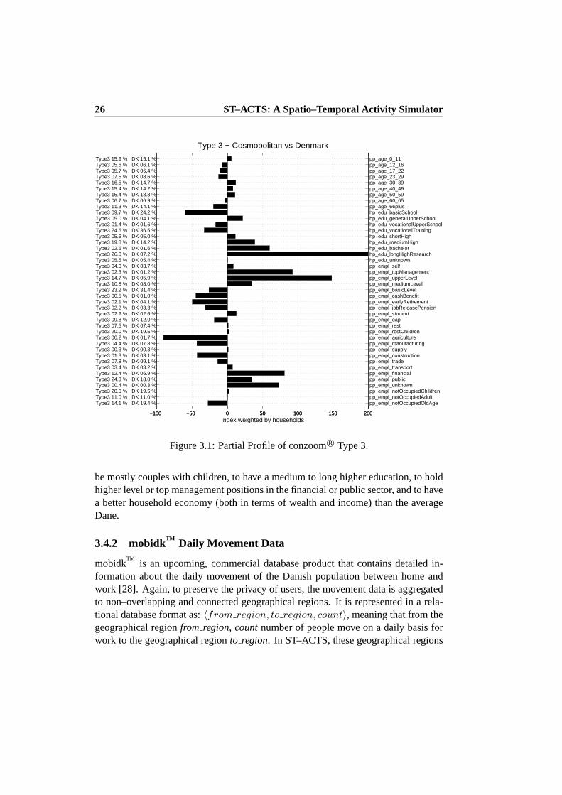
26 ST–ACTS: A Spatio–Temporal Activity Simulator
−100 −50 0 50 100 150 200
pp_age_0_11pp_age_12_16pp_age_17_22pp_age_23_29pp_age_30_39pp_age_40_49pp_age_50_59pp_age_60_65pp_age_66plushp_edu_basicSchoolhp_edu_generalUpperSchoolhp_edu_vocationalUpperSchoolhp_edu_vocationalTraininghp_edu_shortHighhp_edu_mediumHighhp_edu_bachelorhp_edu_longHighResearchhp_edu_unknownpp_empl_selfpp_empl_topManagementpp_empl_upperLevelpp_empl_mediumLevelpp_empl_basicLevelpp_empl_cashBenefitpp_empl_earlyRetirementpp_empl_jobReleasePensionpp_empl_studentpp_empl_oappp_empl_restpp_empl_restChildrenpp_empl_agriculturepp_empl_manufacturingpp_empl_supplypp_empl_constructionpp_empl_tradepp_empl_transportpp_empl_financialpp_empl_publicpp_empl_unknownpp_empl_notOccupiedChildrenpp_empl_notOccupiedAdultpp_empl_notOccupiedOldAge
Type 3 − Cosmopolitan vs Denmark
Index weighted by households−100 −50 0 50 100 150 200
Type3 15.9 % DK 15.1 %Type3 05.6 % DK 06.1 %Type3 05.7 % DK 06.4 %Type3 07.5 % DK 08.6 %Type3 16.5 % DK 14.7 %Type3 15.4 % DK 14.2 %Type3 15.4 % DK 13.8 %Type3 06.7 % DK 06.9 %Type3 11.3 % DK 14.1 %Type3 09.7 % DK 24.2 %Type3 05.0 % DK 04.1 %Type3 01.4 % DK 01.6 %Type3 24.5 % DK 36.5 %Type3 05.6 % DK 05.0 %Type3 19.8 % DK 14.2 %Type3 02.6 % DK 01.6 %Type3 26.0 % DK 07.2 %Type3 05.5 % DK 05.4 %Type3 04.0 % DK 03.7 %Type3 02.3 % DK 01.2 %Type3 14.7 % DK 05.9 %Type3 10.8 % DK 08.0 %Type3 23.2 % DK 31.4 %Type3 00.5 % DK 01.0 %Type3 02.1 % DK 04.1 %Type3 02.2 % DK 03.3 %Type3 02.9 % DK 02.6 %Type3 09.8 % DK 12.0 %Type3 07.5 % DK 07.4 %Type3 20.0 % DK 19.5 %Type3 00.2 % DK 01.7 %Type3 04.4 % DK 07.8 %Type3 00.3 % DK 00.3 %Type3 01.8 % DK 03.1 %Type3 07.8 % DK 09.1 %Type3 03.4 % DK 03.2 %Type3 12.4 % DK 06.9 %Type3 24.3 % DK 18.0 %Type3 00.4 % DK 00.3 %Type3 20.0 % DK 19.5 %Type3 11.0 % DK 11.0 %Type3 14.1 % DK 19.4 %
Figure 3.1: Partial Profile of conzoomR© Type 3.
be mostly couples with children, to have a medium to long higher education, to holdhigher level or top management positions in the financial or public sector, and to havea better household economy (both in terms of wealth and income) than the averageDane.
3.4.2 mobidkTM
Daily Movement Data
mobidkTM
is an upcoming, commercial database product that contains detailed in-formation about the daily movement of the Danish population between home andwork [28]. Again, to preserve the privacy of users, the movement datais aggregatedto non–overlapping and connected geographical regions. It is represented in a rela-tional database format as:〈from region, to region, count〉, meaning that from thegeographical regionfrom region, countnumber of people move on a daily basis forwork to the geographical regionto region. In ST–ACTS, these geographical regions

3.5 ST–ACTS: Spatio–Temporal ACTivity Simulator 27
are parishes, which on average contain 1176 households, and 195 100–meter gridcells1.
3.4.3 bizmarkTM
Business Data
bizmarkTM
is a commercial database product that contains detailed information aboutDanish businesses both in the public and the private sector [28]. Some of the one–to–one information that is available about businesses is their location, the number ofemployees working in them, the physical size of the business facility, and the inter-national branch codes the businesses fall under. Detailed but aggregated informationabout the employees within businesses is also available for appropriate bizmark
TM
clusters, which are constructed taking into account geography, business branch, busi-ness size in term of number of employees and physical size of the businessfacility,and various other descriptive business variables.
3.4.4 GallupPCR© Consumer Survey Data
GallupPCR© is a commercial database product and as the name suggests, it containsdetailed survey responses of consumers about their demographics; interests such asculture, hobbies, and sports; household consumptions, purchasing habits; transporta-tion habits; views on various subjects; attitudes and exposure to various advertise-ment media [26]. The questions in the surveys are yes/no questions. To measure themagnitude of the response of an individual survey subject to a specific question, theoriginal yes/no question is re–phrased with a reference to a time–frequency interval.For example the original yes/no question “Do you go to the library?” is re–phrasedto 7 yes/no questions using the following time–frequency intervals: daily / almostdaily; 3-4 times a week; 1-2 times a week; 1-3 times a month; 1-5 times every 6month; seldom, and never.
3.5 ST–ACTS: Spatio–Temporal ACTivity Simulator
In this section, main components of ST–ACTS and their use of the source dataisdescribed. In the description a simulated person, who performs activities intimeand space, will be abbreviated as a simperson. A MATLAB toolbox for ST–ACTScan be downloaded for research purposes fromhttp://www.geomatic.dk/research/ST--ACTS/ .
1The commercial version of mobidkTM
contains the same information for smaller, neighborhoodclusters that on average contain 230 households and 38 100–meter gridcells.

28 ST–ACTS: A Spatio–Temporal Activity Simulator
hp_persIncome_0_20
hp_persIncome_20_40
hp_persIncome_40_60
hp_persIncome_60_80
hp_persIncome_80_100
hp_edu_basicSchool
hp_edu_generalUpperSchool
hp_edu_vocationalUpperSchool
hp_edu_vocationalTraining
hp_edu_shortHigh
hp_edu_mediumHigh
hp_edu_bachelor
hp_edu_longHighResearch
hp_edu_unknown −0.6
−0.4
−0.2
0
0.2
0.4
0.6
Figure 3.2: Correlation between education and income.
3.5.1 Drawing Demographic Variables for Simpersons
The conzoomR© source data contains accurate, detailed demographic informationabout the population aggregated to a cluster level. As described in Section 3.4.1,continuous variables are discretized into categories. Clusters contain counts for allcategories for all variables. Having the exact number of persons, housing units, andhouseholds at a grid cell level, and assuming the same distribution of variables in theindividual grid cells as in the cluster they belong to, counts for all categories for allvariables are calculated at a grid cell level. A simperson is assigned a category fora given variable proportional to the counts of the categories for the given variable inthe grid cell the simperson lives in. In short, a category for the variable is assigned tothe simperson according to the distribution of the variable. To draw assign categoriesfor variables without replacement, corresponding counts in the given grid cell aredecremented. Since counts of some of the variables in the grid cell refer to entitiesother than persons, but are variables that are part of the demographicvariables thatdescribe a person, these counts are adjusted to sum to the number of persons in thecell.
3.5.2 Skewing Distributions Based on Correlations
The above described method for assigning categories for demographic variables hasone major flaw: demographic variables are not independent. For example the edu-cation type variable has a strong correlation with the personal income variable. Thiscorrelation is illustrated in Figure 3.2. Correlations are calculated between theper-centages of the categorized variables, and samples are weighted by the number ofpersons in the cells. From the colorbar on the side one can see that darker shadesmean stronger negative correlations and lighter shades mean stronger positive corre-

3.5 ST–ACTS: Spatio–Temporal ACTivity Simulator 29
1 2 3 4 5 6 7 8 905
10Distribution of variable group: p_age −− [Selected: 5]
1 2 3 4 5 6 7 8 90
0.2
Distribution of variable group: p_edu
1 2 3 4 5 6 7 8 9−0.5
00.5
Raw correlations for p_edu given p_age = 5
1 2 3 4 5 6 7 8 9012
Normalized correlations for p_edu given p_age = 5
1 2 3 4 5 6 7 8 90
0.2
Skewed distribution for p_edu given p_age = 5 −− [Selected: 4]
1 2 3 4 5 6 7 8 9 10 11 120
0.2
Distribution of variable group: p_emplState
1 2 3 4 5 6 7 8 9 10 11 12012
Normalized correlations for p_emplState given p_edu = 4
1 2 3 4 5 6 7 8 9 10 11 12012
Joint normalized correlations for p_emplState given p_age = 5, p_edu = 4
1 2 3 4 5 6 7 8 9 10 11 120
0.2
Skewed distribution for p_emplState given p_age = 5, p_edu = 4 −− [Selected: 11]
Figure 3.3: Drawing Samples Without Replacement from Correlated, MultivariateDistributions.
lations. The correlations support the common knowledge that people havinghighereducation levels tend to have better paying jobs. Similar correlations exist betweenother variables.
To remedy the above described flaw, which could result in unrealistic assignmentof categories for variables to simpersons, the assignment is modified by drawing cat-egories from skewed variable distributions that try to embed the correlationsbetweenthe variables as follows. For a given simperson, the category for the first variable,age, is drawn without replacement from unskewed distribution of the age variable.An example of this distribution and the result of the draw is shown in the top mostleft subgraph of Figure 3.3, where for the age variable the category 5 was drawn,which represents that the simperson is in the age group 30–39. The distribution ofthe second variable, education, is shown in the second–from–top left subgraph ofFigure 3.3. Given this distribution, categories 4, 6 and 8 are most likely to be as-signed to the simperson for the education variable. However, the correlations (shownin the third left subfigure of Figure 3.3) between the age category 5 and educationvariable reveal positive correlations for categories 1 and 4, and a negative correlationfor category 8 for the education variable. After normalizing (shifting to mean1) thecorrelations, the original distribution of the education variable is skewed bypair–wisemultiplying the raw counts of categories of the education variable and the normalizedcorrelations for the education variable given that the age category of thesimpersonis 5. This skewed distribution is shown in the bottom left subgraph of Figure 3.3 andis used for sampling the education variable, resulting in the education category 4,vocational training. Values for further variables are drawn from skewed distributions

30 ST–ACTS: A Spatio–Temporal Activity Simulator
that take into account the categories for the previously drawn variables,by skewingthe distribution of the current variable by the average of the normalized correlationsfor the so far drawn categories. This process is shown from top to bottomon the rightsubfigures of Figure 3.3, where given that the age category a the simperson is 5 andthe education category is 4 for the third variable, employment state, the category 11is drawn.
3.5.3 Assigning Simpersons to Work Places / Schools
Activities can be divided into two groups:free time activitiesandmandatory activ-ities. While the notion of “mandatory” activity may differ from person to person,for the purposes of simulation, ST–ACTS considers going toschooland work asmandatory activities. The rest of the activities in ST–ACTS are consideredfree timeactivities.
With respect to mandatory activities, simpersons can be divided into three groups:retired, worker, and student. For the retired simpersons, it can be assumed that theyenjoy the fruits of a hard–working life and have no mandatory activities. Conse-quently, they spend the majority of the time either at home or performing free timeactivities. The following paragraphs describe the methods in ST–ACTS (and theirusage of the base data) for assigning simpersons in the worker and student groups totheir work places and schools respectively.
Assigning Worker Simpersons to Work Places:Simpersons in the worker groupare assigned towork placesin two steps. In the first step, given thehome parishand employment branch of the simperson, the parish–to–parish commuting probabil-ities, and the spatial distribution of businesses in branches, awork parishis assignedto the simperson. In the second step, given the employment branch that the sim-person works in, businesses in the same branch that are located in the work parishof the simperson are retrieved from bizmark
TM. Finally, proportional to the number
of employees that work in the selected businesses, the simperson is probabilisticallyassigned to one of the businesses / work places.
Assigning Student Simpersons to Schools:Simpersons in the student group areassigned to schools in two steps. In the first step, depending on the age group of thesimperson, he or she is assigned to either one of the four educational institution types,or is assigned to be “not in school” and hence is considered to a member of the workergroup. In the second step, educational institutions of the simpersons’s educationalinstitution type are retrieved from bizmark
TM, and the simperson is assigned to the
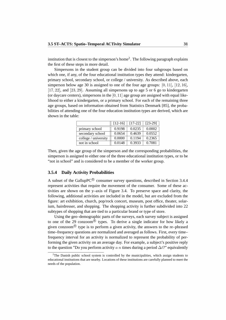
3.5 ST–ACTS: Spatio–Temporal ACTivity Simulator 31
institution that is closest to the simperson’s home2. The following paragraph explainsthe first of these steps in more detail.
Simpersons in the student group can be divided into four subgroups based onwhich one, if any, of the four educational institution types they attend: kindergarten,primary school, secondary school, or college / university. As described above, eachsimperson below age 30 is assigned to one of the four age groups:[0, 11], [12, 16],[17, 22], and[23, 29]. Assuming all simpersons up to age 5 or 6 go to kindergarten(or daycare centers), simpersons in the[0, 11] age group are assigned with equal like-lihood to either a kindergarten, or a primary school. For each of the remaining threeage groups, based on information obtained from Statistics Denmark [85], the proba-bilities of attending one of the four education institution types are derived, which areshown in the table:
[12-16] [17-22] [23-29]
primary school 0.9198 0.0235 0.0002secondary school 0.0654 0.4639 0.0552college / university 0.0000 0.1194 0.2365not in school 0.0148 0.3933 0.7081
Then, given the age group of the simperson and the corresponding probabilities, thesimperson is assigned to either one of the three educational institution types, or to be“not in school” and is considered to be a member of the worker group.
3.5.4 Daily Activity Probabilities
A subset of the GallupPCR© consumer survey questions, described in Section 3.4.4represent activities that require the movement of the consumer. Some of these ac-tivities are shown on the y–axis of Figure 3.4. To preserve space and clarity, thefollowing, additional activities are included in the model, but are excluded from thefigure: art exhibition, church, pop/rock concert, museum, post office, theater, solar-ium, hairdresser, and shopping. The shopping activity is further subdivided into 22subtypes of shopping that are tied to a particular brand or type of store.
Using the geo–demographic parts of the surveys, each survey subjectis assignedto one of the 29 conzoomR© types. To derive a single indicator for how likely agiven conzoomR© type is to perform a given activity, the answers to the re–phrasedtime–frequency questions are normalized and averaged as follows. First,every time–frequency interval for an activity is normalized to represent the probability of per-forming the given activity on an average day. For example, a subject’s positive replyto the question ”Do you perform activitya n times during a period∆t?” equivalently
2The Danish public school system is controlled by the municipalities, which assign students toeducational institutions that are nearby. Locations of these institutions are carefully planned to meet theneeds of the population.

32 ST–ACTS: A Spatio–Temporal Activity Simulator
fitness classical discotheque cinema library0
0.002
0.004
0.006
0.008
0.01
0.012pr
obab
ility
Average DaneMulticultural metropolitanCareer starterMulticultural suburbianActive senior citizenRetired farmerCollege / student hostel
Figure 3.4: Sample Daily Activity Probabilities.
means that the probability of that subject to perform activitya on any given day isP (a) = n/day(∆t), whereday is a function that returns the number of days inperiod∆t. P (a) is equivalently referred to as theDaily Activity Probability(DAP)of activity a. Second, these daily activity probabilities of individual subjects of agiven conzoomR© type are averaged. Figure 3.4 shows a sample of these daily ac-tivity probabilities for a subset of the conzoomR© types. From the figure it can beseen, for example, that a college student is most likely to go to a library, a cinema, adiscotheque, or a fitness center; while a retired farmer is the least likely to performthese activities. Since the figure has the same probability scale, it also reveals that,depending on type, going to a fitness center is about a 7 to 22 times more frequentor popular activity as going to classical concerts. As mentioned before, ST–ACTSincludes the daily activity probabilities of 35 activities for 29 conzoomR© types.
3.5.5 Activity Simulation with Spatio–Temporal Constraints
A simple, random, discrete event activity simulator can be constructed as follows. Atevery time step, a random subset of the simpersons is chosen to perform an activity.Then, for each selected simperson, given his/her conzoomR© type and the associateddaily activity probabilities, an activity is assigned. Then, each selected simperson ismoved to the closest facility, where his/her assigned activity can be performed. Thissimple simulator does not model several spatio–temporal constraints on the activi-ties. In the following, these constraints are discussed, and for each, theproposedmodelling solution that ST–ACTS implements is presented.

3.5 ST–ACTS: Spatio–Temporal ACTivity Simulator 33
Temporal Activity Constraint: Certain activities are more likely to be performedduring specific periods than others. For example, people in the work force tend toleave their homes for work at the beginning of a workday. Consequently,the samepeople are less likely to go to a discotheque, which is presumably closed, during thesame period. To model theTemporal Activity Constraint(TAC), ST–ACTS allowsthe user to define for each of the three population groups the probabilities for eachof the activities for every hour of every day of the week. These probabilities areused to limit the ability of the simperson to perform certain activities during certaintime periods. They are not to be confused with the conzoomR© type dependentdailyactivity probabilities, which encode the activity preference of each type. Throughthe TACs ST–ACTS allows the modelling of opening hours, and to some degreesequential patterns. The TACs of an activity are defined by a 7 by 24 matrix, wherecolumns represent hours of the day, and rows represent days of theweek.
Activity Duration Constraint: Not all activities take the same amount of time. Forexample people usually work 6-10 hours, spend about 2 hours in a cinema, and 30minutes in a grocery store. To model this, from the starting timestamp of an ac-tivity a that is assigned to a simpersons, s becomesoccupiedfor δoccupied (a) timesteps. During this periods is not assigned any other activities. In ST–ACTS,Activ-ity Duration Constraint(ADC) for each activity are probabilistically drawn from theuser–defined activity duration distributions, which is normally distributed with meanµδoccupied (a) and varianceσδoccupied (a).
Minimum Elapsed Time Between Activity Repetition Constraint: While peopleprefer some activities over others, it is very unlikely that they would repeat the same,even if preferred, activity many times, one–after–the–other within a shortperiod. Forexample, it is very unlikely, that even a very active simperson, right afterfinishing hisworkout at the fitness center, decides to go to a fitness center again. Thisconstraint ismodelled in ST–ACTS through the user–definedδelapsed(a), activity–dependentMin-imum Elapsed Time Constraint(METC). The constraint is enforced by maintaining arecent history of activities for each simperson and validating newly drawnactivitiesagainst it.
Maximum Distance Constraint: For most activities there is amaximum distanceaperson is willing to travel. This maximum distance represents a spatial constraint onthe activities that a simpersons will perform, given the current location ofs and thelocations of facilities, where a selected activitya can be performed. Hence, duringthe simulation if there is no suitable facility fora within maximum distance of thecurrent location ofs, the activity is considered invalid fors, ands becomes idle.TheMaximum Distance Constraint(MDC) is controlled by a user–defined, activity–dependent parameter in ST–ACTS.

34 ST–ACTS: A Spatio–Temporal Activity Simulator
(0) //geo–demographic data (conzoomR©): D
(0) //population movement data (mobidkTM
): M
(0) //business data (bizmarkTM
): B
(1) procedureST–ACTS(T ,∆T ,DAP ,TAC ,ADC ,METC ,MDC )
(2) s.dem ← drawDemographicVariables(D)(3) s.work ← simpsToWork(s,B,M )(4) s.acts ← initSimpsActs(s,t=1)(5) for t = 1. . .T(6) free ← unoccupiedSimps(s.acts ,t)(7) a ← validActsToFreeSimps(s,DAP ,TAC ,METC ,t)(8) [f, d] ← facilitiesForActs(a,s,MDC ,B)(9) δoccupied ← durationsOfActs(a,ADC )(10) δtrans ← transitionTimes(d,speed(d))(11) s.acts ← updateSimps(a,f .loc,δoccupied,δtrans,t)
Figure 3.5: Discrete Event Simulation in ST–ACTS.
Physical Mobility Constraint: To move from one location to another takes time.While detailed simulation of this movement is not an objective of ST–ACTS, ba-sic physical mobility constraints are modelled. After a facilityf for an activityais selected for a simpersons, s is moved afterδtrans time steps to the new loca-tion. δtrans is calculated based on the Euclidian distanced in km between the currentlocation ofs and the location of facilityf , assuming a constant speed. This con-stant speed, in km/h, is probabilistically drawn from the distributionspeed(d) =max(5, N(3d, d2)). speed(d) assigns lower speeds to shorter, and higher speeds(with larger variance) to longer distances. It, to some extent, captures common modesof transportation, i.e., people tend to walk on shorter trips, use public transportationor bicycle on slightly longer trips, and use a car or commuting train on even longertrips.
3.5.6 Discrete Event Simulation
Using the conceptual building blocks presented so far, the discrete event simulationperformed in ST–ACTS can be summarized as shown in Figure 3.5. The firstthreecomments indicate that named data sets are used in the simulation, but are not user–defined parameters of it. Arguments to ST–ACTS, shown on line 1, are the user–defined parameters that have been described in the previous paragraphs. On line 2demographic variables are assigned to simpersons based on skewed variable distri-butions. On line 3 simpersons are assigned to work places and schools. Online 4,at time stept = 1 (Monday, 00:00) all simpersons are initialized to be at “home”

3.6 Evaluation of the Simulation 35
0 0.5 1 1.5 2 2.5 3
x 105
0
20
number of simpersons
min
utes
0 0.5 1 1.5 2 2.5 3
x 105
0
5
I/O time
CPU time
Figure 3.6: CPU and I/O Times for Simulations.
doing activity “home to stay” until the early morning hours. Following these prepro-cessing steps, at every time stept, on line 6, currently unoccupied (free) simpersonsare found. Then, on line 7 for each free simperson a valid action is foundaccord-ing to the daily activity probabilities (DAP) of actions for the conzoomR© type ofthe simperson. Actions are valid, if they both meet the temporal activity constraint(TAC) and the minimum elapsed time constraint (METC). On line 8 valid facilitiesare found for these valid activities. Facilities are valid if they meet the maximum dis-tance constraint (MDC). On line 9, activity durations are drawn that meet the activityduration constraint (ADC). On line 10, according to the distances to the assignedactivities, transition times are calculated. Finally, on line 11, information about thenewly assigned activities are stored and the activity histories are updated for the af-fected simpersons.
3.6 Evaluation of the Simulation
ST–ACTS was implemented and tested in MATLAB running on Windows XP on a3.6GHz Pentium 4 processor with 1.5 GB main memory. The geographical extentof ST–ACTS was restricted to the municipalities of Copenhagen and Frederiksbergin Denmark. In this extent, the number of simpersons is 590,050 (178,826 retired,268,615 workers, and 142,609 students), the number of working placesis 1,264,129in 193,299 businesses, and the number of facilities is 10,544. Simulation experimentswere performed for a time step length of∆T = 5 minutes. To test the performanceof ST–ACTS, in all experiments “strict” TACs were set on the two most likely activ-ities, go “home to visit” and go “home to stay”. TACs of other activities were settomodel opening hours of corresponding facilities. As a result a simpersonperformson average9.6 ± 3.2 activities per day.
To evaluate the effectiveness of ST–ACTS, simulations were performed for vary-ing sizes of randomly selected subsets of simpersons during the course ofa single day(24 hours). Figure 3.6 shows both the CPU times (right y–axis) and the I/O timefor

36 ST–ACTS: A Spatio–Temporal Activity Simulator
logging the events (left y–axis). Both of these quantities scale approximatelylinearlywith the number of simpersons. In short, the simulation is fast and scales well.
In a larger experiment activities of the total population for the course of a fullweek have been simulated. The table below shows the output of ST–ACTS for acosmopolitan type simperson during the course of a day.
a.begin a.loc(x) a.loc(y) a.end a.name
8:35 722941 6172634 15:50 work / school17:05 720408 6173933 17:45 Fakta18:55 721350 6177550 20:20 home to visit20:45 723555 6175390 21:10 solarium21:50 723483 6175299 23:30 cinema23:40 721350 6177550 8:25 home to stay
The simulation, without logging the individual events and only keeping statisticsabout activities, took 98 minutes. To evaluate the validity of ST–ACTS, the gath-ered statistics have been analyzed. Due to space limitation, only some results ofthisanalysis are discussed in detail, while others are only summarized.
To evaluate ST–ACTS’s ability to generate the correct distribution of activities,the input DAPs have been compared to the simulated DAPs, shown in Figure 3.7.While, due to the previously mentioned “strict” TACs, the simulated DAPs are about4 times higher than the input DAPs, the relative simulated DAPs among activities issimilar to the input DAPs. By using less “strict” TACs, i.e.: allowing simpersons togo home earlier after work, the scale of simulated DAPs match that of the input DAPs.Differences in the relative DAPs can be explained by the effects of spatio–temporalconstraints on activities.
0
0.02
0.04
0.06
0.08
0.1
0.12
0
0.005
0.01
0.015
0.02
0.025
0.03
Aldi
Bilk
aBo
dy S
hop
Dag
li’ Br
ugse
nfit
ness
cen
ter
Fakt
aFø
tex
sola
rium
art e
xhib
ition
chur
ch
clas
sica
l con
cert
pop
/ roc
k co
ncer
tdi
scot
eque
mus
eum
post
offi
ceci
nem
aha
irdre
sser
libra
ryth
eatre
Gul
dbag
eren
Illum Irm
aIS
OKv
ickl
yKv
ickl
y Xt
raM
agas
inM
atas
Net
toPh
arm
acy
Sallin
gSc
hlec
ker
Spar
/Sup
ersp
ar
Supe
r Bru
gsen
Supe
rBes
t
shop
ping
cen
ter
input DAPssimulated, spatio−temporally constrained DAPs
Figure 3.7: Input and Simulated DAPs.
To evaluate ST–ACTS’s ability to control temporal constraints on activities, countsfor each assigned activity for every hour–of–day and day–of–week were maintained.Figure 3.8 shows the average number of assigned activities for each hour–of–day av-eraged over the days–of–week. Due to the large variation in frequencycounts for

3.6 Evaluation of the Simulation 37
Log−frequency counts for group retired averaged for a week
hour
of t
he d
ay
Aldi
Bilk
aBo
dy S
hop
Dag
li’ Br
ugse
nfit
ness
cen
ter
Fakt
aFø
tex
sola
rium
art e
xhib
ition
chur
ch
clas
sica
l con
cert
pop
/ roc
k co
ncer
tdi
scot
eque
mus
eum
post
offi
ceci
nem
aha
irdre
sser
libra
ryth
eatre
Gul
dbag
eren
Illum Irm
aIS
OKv
ickl
yKv
ickl
y Xt
raM
agas
inM
atas
Net
toPh
arm
acy
Sallin
gSc
hlec
ker
Spar
/Sup
ersp
arSu
per B
rugs
enSu
perB
est
shop
ping
cen
ter
wor
k / s
choo
lho
me
to v
isit
hom
e to
sta
yin
tran
sitio
nid
le
5
101520
Log−frequency counts for group student averaged for a week
hour
of t
he d
ay
Aldi
Bilk
aBo
dy S
hop
Dag
li’ Br
ugse
nfit
ness
cen
ter
Fakt
aFø
tex
sola
rium
art e
xhib
ition
chur
ch
clas
sica
l con
cert
pop
/ roc
k co
ncer
tdi
scot
eque
mus
eum
post
offi
ceci
nem
aha
irdre
sser
libra
ryth
eatre
Gul
dbag
eren
Illum Irm
aIS
OKv
ickl
yKv
ickl
y Xt
raM
agas
inM
atas
Net
toPh
arm
acy
Sallin
gSc
hlec
ker
Spar
/Sup
ersp
arSu
per B
rugs
enSu
perB
est
shop
ping
cen
ter
wor
k / s
choo
lho
me
to v
isit
hom
e to
sta
yin
tran
sitio
nid
le
5
10
15
20
Log−frequency counts for group worker averaged for a week
hour
of t
he d
ay
Aldi
Bilk
aBo
dy S
hop
Dag
li’ Br
ugse
nfit
ness
cen
ter
Fakt
aFø
tex
sola
rium
art e
xhib
ition
chur
ch
clas
sica
l con
cert
pop
/ roc
k co
ncer
tdi
scot
eque
mus
eum
post
offi
ceci
nem
aha
irdre
sser
libra
ryth
eatre
Gul
dbag
eren
Illum Irm
aIS
OKv
ickl
yKv
ickl
y Xt
raM
agas
inM
atas
Net
toPh
arm
acy
Sallin
gSc
hlec
ker
Spar
/Sup
ersp
arSu
per B
rugs
enSu
perB
est
shop
ping
cen
ter
wor
k / s
choo
lho
me
to v
isit
hom
e to
sta
yin
tran
sitio
nid
le
5
10
15
20
0
5
10
0
5
10
0
5
10
Figure 3.8: Validity of ST–ACTS in Terms of TACs.
different activities in different periods of the day, the base 2 logarithm of frequencycounts are shown. From the figure it can be seen that certain groups perform certainactivities at certain times of the day more frequently than other groups. For exam-ple, it can be seen that the retired group is more likely to perform activities duringworking hours, simply because they are free to do so. Opening and closing timesof facilities is also controlled by the parameters. For example, no one goes to dis-cotheques during the day, and no one goes to shopping centers in the middleof thenight.
To evaluate ST–ACTS’s ability to control spatial constraints on activities, thedaily distance travelled to work by an average simperson (2.7±2.3 km) was comparedto the total daily distance travelled by an average simperson (8.3 ± 3.6 km). Whilefor the same numbers no ground truth was available to evaluate against, consideringthe average 9.6 activities per day the numbers seem reasonable. The simulated datahas also been verified that no trips violate the activity–dependent maximum distancecriteria.
38 ST–ACTS: A Spatio–Temporal Activity Simulator
3.7 Conclusions and Future Work
Realistic models that simulate the spatio–temporal activities of users, and hencethedistribution of moving objects, are essential to facilitate the development of ade-quate spatio–temporal data management and data mining techniques. In this paper,ST–ACTS, the first of such simulators is presented. Experimental results show that,using a number of real–world geo–statistical data sources and intuitive principles,ST–ACTS is able to effectively generate realistic spatio–temporal activity data. Itis also demonstrated that the generated data has the same characteristics as itis de-fined by the user–controllable model parameters. ST–ACTS has been implementedin MATLAB and is available for research purposes.
While the correspondence between the characteristics of the generated data andthe model parameters is demonstrated, the accuracy of the simulation has to be nec-essarily affected by the limited modelling of physical aspects of mobility. Hence infuture work, integrating the output of ST–ACTS as an input to sophisticatednetwork–based moving object simulation as in [8] is planned. Such a more complex simulatorwill provide synthetic data sets that can aid the development in telematics, intelligenttransportation systems, and location–based services.
Chapter 4
Mining Long, Sharable Patterns inTrajectories of Moving Objects
The efficient analysis of spatio–temporal data, generated by moving objects, is anessential requirement for intelligent location–based services. Spatio–temporal rulescan be found by constructing spatio–temporal baskets, from which traditional associ-ation rule mining methods can discover spatio–temporal rules. When the items in thebaskets are spatio–temporal identifiers and are derived from trajectories of movingobjects, the discovered rules represent frequently travelled routes. For some applica-tions, e.g., an intelligent ride–sharing application, these frequent routes are only in-teresting if they are long and sharable, i.e., can potentially be shared by several users.This paper presents a database projection based method for efficiently extracting suchlong, sharable frequent routes. The method prunes the search spaceby making useof the minimum length and sharable requirements and avoids the generation of theexponential number of sub–routes of long routes. Considering alternative modellingoptions for trajectories, leads to the development of two effective variantsof the me-thod. SQL–based implementations are described, and extensive experiments on bothreal life– and large–scale synthetic data show the effectiveness of the method and itsvariants.
4.1 Introduction
In recent years Global Positioning Systems (GPS) have become increasingly avail-able and accurate in mobile devices. As a result large amounts of spatio–temporaldata is being generated by users of such mobile devices, referred to asmoving ob-
39

40 Mining Long, Sharable Patterns in Trajectories of Moving Objects
jects in the following. Trajectories of moving objects, or trajectories for short, con-tain regularities or patterns. For example, a person tends to drive almost every week-day to work approximately at the same time using the same route. The benefits offinding such regularities or patterns is many–fold. First, such patterns canhelp theefficient management of trajectories. Second, they can be used to facilitatevariousLocation–Based Services (LBS). One LBS example is an intelligent rideshare appli-cation, which finds sharable routes for a set of commuters and suggests ridesharepossibilities to them, is considered. Such a rideshare application can be one possiblesolution to the ever increasing congestion problems of urban transportationnetworks.
Patterns in trajectories for an intelligent rideshare application are only interest-ing if those patterns are sharable by multiple commuters, are reoccurring frequently,and are worthwhile pursuing, i.e., are long enough for the savings to compensate forthe coordination efforts. The discovery of Long, Sharable Patterns (LSP) in trajec-tories is difficult for several reasons. Patterns do not usually exist along the wholetrajectory. As a example, consider two commutersA andB living in the same areaof town, leaving for work approximately the same time, and working in the samepart of town. Given the underlying road network and traffic conditions,for a givensupport threshold the middle part of the trips of the two commuters may be frequent,the initial and final parts may not. In recent work [30] a general problemtransforma-tion method, calledpivoting, was proposed for the analysis of spatio–temporal data.Pivoting is the process of grouping a set of records based on a set ofattributes andassigning the values of likely another set of attributes to groups or baskets. Pivotingapplied to spatio–temporal data allows the construction of spatio–temporal baskets,which can be mined with traditional association rule mining algorithms. When theitems in the baskets are spatio–temporal identifiers and are derived from trajectories,the discovered rules represent frequently travelled routes. While thereexist severalefficient association rule mining methods [40], the straight–forward application ofthese algorithms to spatio–temporal baskets representing trajectories is infeasible fortwo reasons. First, all sub–patterns of frequent patterns are also frequent, but notinteresting, as longer patterns are preferred. Second, the support criterion used inassociation rule mining algorithms is inadequate for a rideshare application, i.e.,afrequent itemset representing a frequent trajectory pattern, may be supported by asingle commuter on many occasions and hence presents no rideshare opportunity.
In this paper, to overcome the above difficulties of finding LSPs in trajectories, anovel method is given. According to a new support criterion, the proposed methodfirst efficiently filters the trajectories to contain only sub–trajectories that are fre-quent. Next, it removes trajectories that do not meet the minimum length criterion.Then it alternates two steps until there are undiscovered LSPs. The firststep entailsthe discovery of a LSP. The second step entails the filtering of trajectories by thepreviously discovered pattern. An advantage of the proposed method is the ease of

4.2 Related Work 41
implementation in commercial Relational Database Management Systems (RDBM-Ses). To demonstrate this, a SQL–based implementation is described. Consideringthe global modelling of trajectories, leads to the development of two other effectivevariants of the proposed method. The effectiveness of the method and its variants aredemonstrated on the publicly available INFATI data, which contains trajectories ofcars driving on a road network, and on a number of large–scale synthetic data sets.
The herein presented work is novel in several aspects. It is the first toconsider theproblem of mining LSPs in trajectories. It describes a novel transformation, and therelationship between the problem of mining LSPs in trajectories and mining frequentitemsets. Finally, it describes an effective method with a simple SQL–implementationto mine such LSPs in trajectories.
The remainder of the paper is organized as follows. Section 4.2 reviews relatedwork. Section 4.3 describes the transformation, the use of the framework infre-quent itemset mining, and formally defines the task of mining LSPs in trajectories.Section 4.4 discusses a naıve method for mining LSPs and points out its shortcom-ings. Section 4.5 describes the proposed algorithm and a SQL–based implementationfor mining LSPs. Section 4.6 presents alternative modelling of trajectories andde-rives variants of the proposed method based on these modelling options. Section 4.7presents detailed experimental results. Finally, Section 4.8 concludes and points tofuture research.
4.2 Related Work
Frequent pattern mining is a core field in data mining research. Since the firstsolu-tion to the problem of frequent itemset mining [1,2], various specialized in–memorydata structures have been proposed to improve the mining efficiency, see [40] for anoverview. It has been recognized that the set of all frequent itemsets istoo large foranalytical purposes and the information they contain is redundant. To remedy this,two modification to the task have been proposed: mining of Closed Frequent Itemsets(CFI) and mining of maximal frequent itemsets. A frequent itemsetX is closedif noitemsetY exists with the same support asX such thatX ⊂ Y . A frequent itemsetXis maximalif no frequent itemsetY exists such thatX ⊂ Y . Prominent methods thatefficiently exploit these modifications to the problem are MAFIA [9], GenMax[42],CLOSET [76], CLOSET(+) [98], and CHARM [104]. Later in the paper, a rela-tionship between the problems of mining LSPs in trajectories and mining CFIs aredescribed. While CFI mining methods can be modified to find the desired solutionthat meets thesharablecriterion, they employ complex data structures and their im-plementation is quite involved; hence their augmentation is difficult. In particular,aprojection–based CFI mining algorithm that employs an in–memory FP–tree to rep-resent itemsets, would need to be modified at every node to maintain a set of distinct

42 Mining Long, Sharable Patterns in Trajectories of Moving Objects
objects at that have transactions associated with them that support the itemset thatis represented by the node. In comparison, the herein presented method –buildingon work presented in [84]–exploits the power of commercial RDBMSs, yielding asimple, but effective solution.
Since trajectories are temporally ordered sequences of locations, sequential pat-tern mining [3] naturally comes to mind. However, a straight forward interpretationof trips as transactions and application of a state–of–the–art closed frequent sequen-tial pattern mining algorithm [103] does not yield the desired solution, since in thiscase sequences of frequent sub–trajectories would be found. Furthermore, since thetrajectories can contain hundreds of items, closedness checking of frequent itemsetseven for prominent methods would be computationally expensive. Interpreting singleelements of trajectories as transactions and applying closed sequential pattern miningcould find frequent sub–trajectories. However a number of problems arise. First, tomeet the sharable criterion, the in–memory data structures would need similar, non–trivial augmentation as described above. Second, since patterns in trajectories couldbe extremely long, even state–of–the–art sequential mining methods [95,103] wouldhave a difficulties handling patterns of such lengths. Third, patterns in trajectoriesrepeat themselves, which cannot be handled by traditional sequential pattern miningalgorithms. The extraction of spatio–temporal periodic patterns from trajectories isstudied in [70], where a bottom–up, level–wise, and a faster top–down miningalgo-rithm is presented. Although the technique is effective, the patterns foundare withinthe trajectory of a single moving object. In comparison, the herein presentedmethodeffectively discovers long, sharable, periodic patterns.
Moving objects databases are particular cases of spatio–temporal databases thatrepresent and manage changes related to the movement of objects. A necessary com-ponent to such databases are specialized spatio–temporal indices such as the Spatio–Temporal R–tree (STR–tree) and Trajectory–Bundle tree (TB–tree) [55]. An STR–tree organizes line segments of a trajectory according to both their spatial propertiesand the trajectories they belong to, while a TB–tree only preserves trajectories. Iftrajectories are projected to the time–of–day domain, STR–tree index values on theprojected trajectories could be used as an alternative representation of trajectories.While this approach would reduce the size of the problem of mining LSPs in tra-jectories, it would not solve it. In comparison, the herein presented method solvesthe problem of mining LSPs in trajectories, which is orthogonal, but not unrelated toindexing of trajectories.
In [97] a way to effectively retrieve trajectories in the presence of noiseis pre-sented. Similarity functions, based on the longest sharable subsequence, are defined,facilitating an intuitive notion of similarity between trajectories. While such an effi-cient similarity search between the trajectories will discover similar trajectories,theusefulness of this similarity in terms of length and support would not be explicit.

4.3 Long, Sharable Patterns in Trajectories 43
0 5 10 15 20 25 30 35 400
5
10
15Mon 8:00
Tu 8:00
Wed 8:00
x−dimension
y−dimension
time−
dim
ensi
on /
date
−tim
e do
mai
n trip 1
trip 2
trip 3
dk > δ → start of trip 1
dk < δ → end of trip 1
(a) Identification of Trips in Raw Trajectories.
0 5 10 15 20 25 30 35 40
0
5
10
158:00
8:05
8:10
8:15
8:00
8:00
8:30
8:35
x−dimensiony−dimension
time−
dim
ensi
on /
time−
of−
day
dom
ain
spatio−temporal region
(b) Time–Of–Day Projection and Spatio–TemporalRegion Substitution.
Figure 4.1: From Trajectories to Transactions.
In comparison, there herein proposed method returns only patterns that meet theuser–specified support and length constraints. Furthermore, the trajectory patternsreturned by the proposed method are explicit, as opposed to the only implicit patternscontained in similar trajectories.
4.3 Long, Sharable Patterns in Trajectories
The following section describes a novel transformation of raw trajectories. This trans-formation allows (1) the formulation of the problem of mining LSPs in trajectoriesin a framework similar to that used in frequent itemset mining, (2) to establish arelationship between the two problems.
4.3.1 From Trajectories to Transactions
The proposed transformation of raw trajectories consists of three steps:identificationof trips, projection of the temporal dimension, and spatio–temporal region substitu-tion. It is assumed that locations of moving objects are sampled over a long history.That is, a raw trajectory is a long sequence of(x, y, t) measurements at regular timeintervals.
Identification of TripsA trip is a temporally consecutive set or sequence of measurements such that for
any measurementmi in the sequence, the sum of spatial displacement during thek measurements immediately followingmi, denoteddk, is larger than some user–defined displacement,δ. Trips can be identified in a straight–forward manner by lin-early scanning through a trajectory, and calculatingdk using a look–ahead window

44 Mining Long, Sharable Patterns in Trajectories of Moving Objects
of k measurements. That is, scanning through the total trajectory from the begin-ning, the first measurement for whichdk > δ, signals the beginning of the first trip.Consecutive measurements are part of this trip until a measurement is reached forwhich dk ≤ δ, which signals the end of the first trajectory. Trips following the firsttrip are detected in the same fashion from the remaining part of the total trajectory.Figure 4.1(a) shows three example trips that are derived from the total trajectory ofone moving object.
Projection of the Temporal DimensionSince frequent patterns within a single object’s trajectory are expected to repeat
themselves daily, the temporal dimension of the so identified trips is projected downto the time–of–day domain. This projection is essential to discover the daily periodicnature of patterns in trajectories. Mining patterns with other periodicity can befa-cilitated by projections of the temporal domain to appropriate finer, or coarser levelsof granularity. Finer levels of granularity can be used to detect patterns with shorterperiodicity. For example, a delivery person might use a different route depending onthe time–of–hour knowing that at the given time of the hour certain traffic conditionsarise, which make an otherwise optimal delivery route sub–optimal. The detectionof these patterns in delivery routes requires the projection of the temporaldimen-sion to the time–of–hour domain. Conversely, coarser levels of granularitycan beused to detect patterns with longer periodicity. For example, a person might visit hisbank only at the end of pay periods. The detection of this pattern requiresthe pro-jection of the temporal dimension to the day–of–month domain. Finally, to discoverthe pattern that the above mentioned person makes these visits to his bank Saturdaymornings following the end of pay periods, requires the projection of the temporaldomain to a combination of the day–of–month, the day–of–week, and the part–of–day domains. Performing different projections is part of the inherently iterative andonly semi–automatic process of doing data mining when the exact format of the pat-terns searched for is not known beforehand. Figure 4.1(b) shows the projection ofthe temporal dimension to the time–of–day domain for the three trips identified inFigure 4.1(a). Since the projection of a single database record is a constant time op-eration, the total processing time of this transformation step is optimal and linear inthe number of database records.
Spatio–Temporal Generalization and SubstitutionTrajectories are noisy. One source of this noise is due to imprecise GPS mea-
surements. From the point of view of patterns in such trajectories, slight deviationof trajectories from the patterns can be viewed as noise. Examples of suchdevia-tions could be due to a few minute delay, or to the usage of different lanes ontheroute. Hence, while a person might be driving from home to work at approximatelythe same time of day using approximately the same route, the chance of two identi-
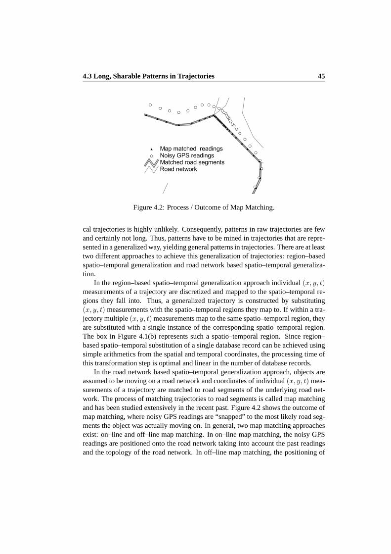
4.3 Long, Sharable Patterns in Trajectories 45
Figure 4.2: Process / Outcome of Map Matching.
cal trajectories is highly unlikely. Consequently, patterns in raw trajectoriesare fewand certainly not long. Thus, patterns have to be mined in trajectories that are repre-sented in a generalized way, yielding general patterns in trajectories. There are at leasttwo different approaches to achieve this generalization of trajectories: region–basedspatio–temporal generalization and road network based spatio–temporal generaliza-tion.
In the region–based spatio–temporal generalization approach individual (x, y, t)measurements of a trajectory are discretized and mapped to the spatio–temporal re-gions they fall into. Thus, a generalized trajectory is constructed by substituting(x, y, t) measurements with the spatio–temporal regions they map to. If within a tra-jectory multiple(x, y, t) measurements map to the same spatio–temporal region, theyare substituted with a single instance of the corresponding spatio–temporal region.The box in Figure 4.1(b) represents such a spatio–temporal region. Since region–based spatio–temporal substitution of a single database record can be achieved usingsimple arithmetics from the spatial and temporal coordinates, the processing timeofthis transformation step is optimal and linear in the number of database records.
In the road network based spatio–temporal generalization approach, objects areassumed to be moving on a road network and coordinates of individual(x, y, t) mea-surements of a trajectory are matched to road segments of the underlying road net-work. The process of matching trajectories to road segments is called map matchingand has been studied extensively in the recent past. Figure 4.2 shows theoutcome ofmap matching, where noisy GPS readings are “snapped” to the most likely road seg-ments the object was actually moving on. In general, two map matching approachesexist: on–line and off–line map matching. In on–line map matching, the noisy GPSreadings are positioned onto the road network taking into account the pastreadingsand the topology of the road network. In off–line map matching, the positioningof
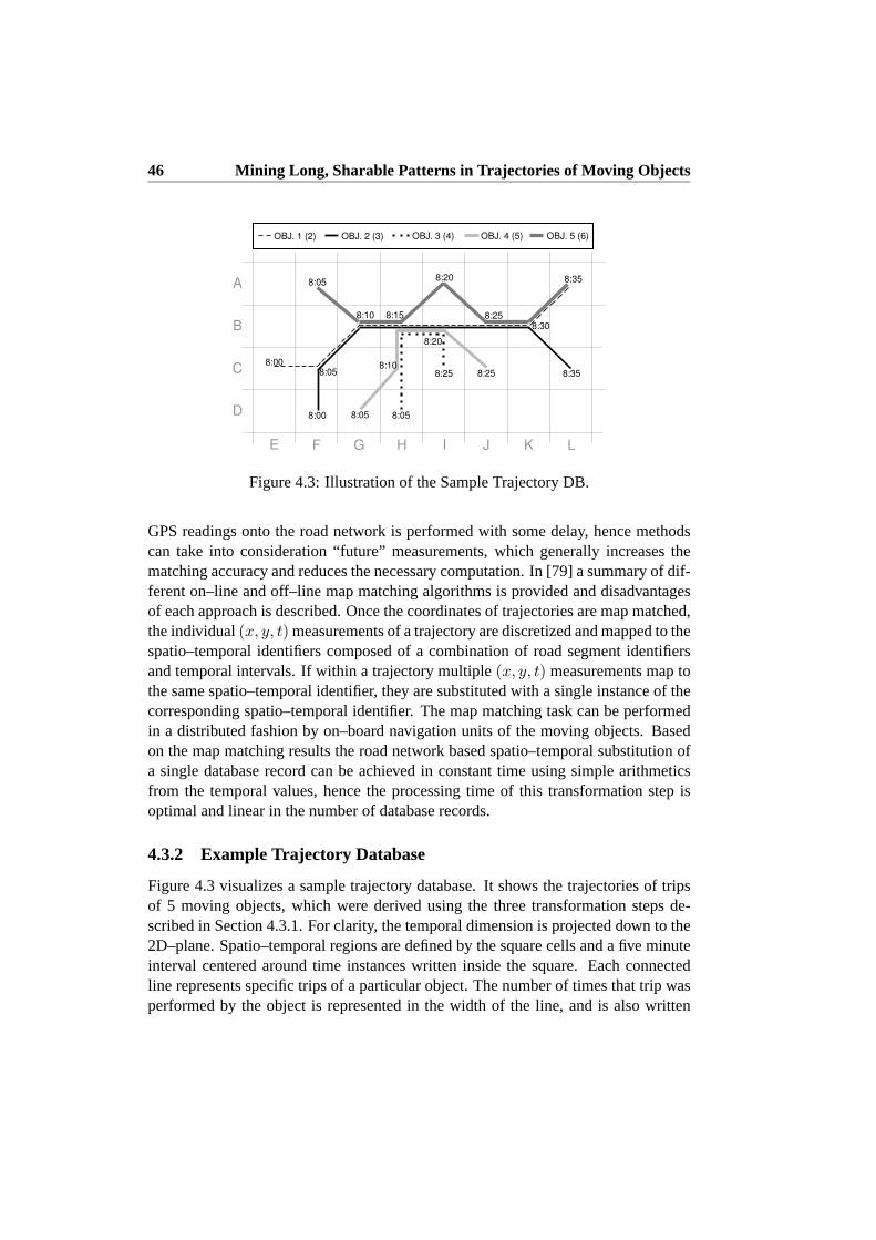
46 Mining Long, Sharable Patterns in Trajectories of Moving Objects
A
C
B
GFE
D
KJIH L
8:00
8:158:10
8:00
8:05
8:058:05
8:10
8:25
8:20
8:25
8:20
8:25
8:35
8:30
8:35
OBJ. 1 (2) OBJ. 5 (6)OBJ. 4 (5)OBJ. 3 (4)OBJ. 2 (3)
8:05
Figure 4.3: Illustration of the Sample Trajectory DB.
GPS readings onto the road network is performed with some delay, hence methodscan take into consideration “future” measurements, which generally increases thematching accuracy and reduces the necessary computation. In [79] a summary of dif-ferent on–line and off–line map matching algorithms is provided and disadvantagesof each approach is described. Once the coordinates of trajectories are map matched,the individual(x, y, t) measurements of a trajectory are discretized and mapped to thespatio–temporal identifiers composed of a combination of road segment identifiersand temporal intervals. If within a trajectory multiple(x, y, t) measurements map tothe same spatio–temporal identifier, they are substituted with a single instance ofthecorresponding spatio–temporal identifier. The map matching task can be performedin a distributed fashion by on–board navigation units of the moving objects. Basedon the map matching results the road network based spatio–temporal substitutionofa single database record can be achieved in constant time using simple arithmeticsfrom the temporal values, hence the processing time of this transformation step isoptimal and linear in the number of database records.
4.3.2 Example Trajectory Database
Figure 4.3 visualizes a sample trajectory database. It shows the trajectoriesof tripsof 5 moving objects, which were derived using the three transformation steps de-scribed in Section 4.3.1. For clarity, the temporal dimension is projected down tothe2D–plane. Spatio–temporal regions are defined by the square cells and afive minuteinterval centered around time instances written inside the square. Each connectedline represents specific trips of a particular object. The number of times that trip wasperformed by the object is represented in the width of the line, and is also written

4.3 Long, Sharable Patterns in Trajectories 47
in parenthesis next to the object name in the legend. For example, the trip trajectoryassociated with object3 was performed4 times by the object. The object was inspatial regions HD, HC, HB, IB, and IC during time intervals8:05 ± 2.5 minutes,8:10± 2.5 minutes,8:15± 2.5 minutes,8:20± 2.5 minutes, and8:25± 2.5 minutes,respectively. In the following a spatio–temporal region will be referred toby its con-catenated values of the cell identifiers along the x– and y–axis, and the correspondingtime instance denoting the center of the time interval of the spatio–temporal region.Hence, trips associated with object3 will be denoted by the a sequenceHD8:05,HC8:10, HB8:15, IB8:20, IC8:25. Furthermore, the trajectory databaseT is as-sumed to be in a relational format with schema〈oid, tid, item〉, whereitem is asingle item, that is part of the transactiontid associated with objectoid. Hence, eachof the four trips of object3 is represented by5 unique rows inT .
4.3.3 Problem Statement
After performing the three above transformation steps, the data set can berepresentedin a databaseT containing tuples〈oid, tid, s〉, whereoid is an object identifier,tidis a trip identifier, ands is a sequence of spatio–temporal region identifiers. Sincespatio–temporal region identifiers contain a temporal component, the sequences can,without loss of information, be represented as asetof spatio–temporal region iden-tifiers. Conforming to the naming convention used in the frequent itemset miningframework, a spatio–temporal region identifier will be equivalently referred to as anitem, and a sequence of spatio–temporal region identifiers will be equivalentlyre-ferred to as atransaction. Let X be a set of items, called anitemset. A transactiontsatisfiesan itemsetX iff X ⊆ t. Let STX denote the set of transactions that satisfyX. The following definitions are emphasized to point out the differences between thefrequent itemset mining framework and the one established here.
Definition 1 Then–support of an itemsetX in T , denoted asX.supp(n), is definedas the number of transactions inSTX if the number of distinctoids associated withthe transactions inSTX is greater than or equal ton, and 0 otherwise. Then–support of an itemi in T , denoted asi.supp(n), is equal to then–support of theitemset that contains onlyi.
Definition 2 Thelength of an itemsetX, denoted as|X|, is defined as the numberof items inX.
Definition 3 An itemsetX is n–frequent in T if X.supp(n) ≥ MinSupp, andXis long if |X| ≥ MinLength, whereMinLength, MinSupp, andn are user–definedvalues.
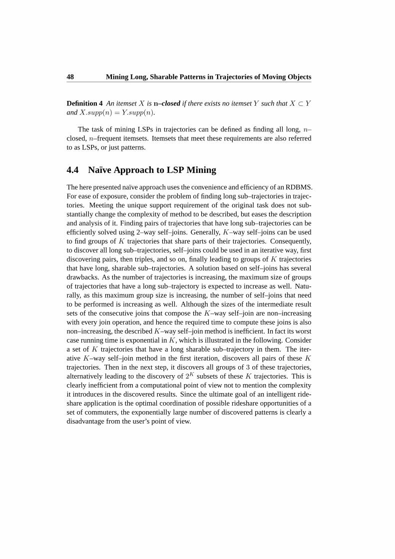
48 Mining Long, Sharable Patterns in Trajectories of Moving Objects
Definition 4 An itemsetX is n–closedif there exists no itemsetY such thatX ⊂ YandX.supp(n) = Y.supp(n).
The task of mining LSPs in trajectories can be defined as finding all long,n–closed,n–frequent itemsets. Itemsets that meet these requirements are also referredto as LSPs, or just patterns.
4.4 Naıve Approach to LSP Mining
The here presented naıve approach uses the convenience and efficiency of an RDBMS.For ease of exposure, consider the problem of finding long sub–trajectories in trajec-tories. Meeting the unique support requirement of the original task does not sub-stantially change the complexity of method to be described, but eases the descriptionand analysis of it. Finding pairs of trajectories that have long sub–trajectories can beefficiently solved using 2–way self–joins. Generally,K–way self–joins can be usedto find groups ofK trajectories that share parts of their trajectories. Consequently,to discover all long sub–trajectories, self–joins could be used in an iterative way, firstdiscovering pairs, then triples, and so on, finally leading to groups ofK trajectoriesthat have long, sharable sub–trajectories. A solution based on self–joinshas severaldrawbacks. As the number of trajectories is increasing, the maximum size of groupsof trajectories that have a long sub–trajectory is expected to increase as well. Natu-rally, as this maximum group size is increasing, the number of self–joins that needto be performed is increasing as well. Although the sizes of the intermediate resultsets of the consecutive joins that compose theK–way self–join are non–increasingwith every join operation, and hence the required time to compute these joins is alsonon–increasing, the describedK–way self–join method is inefficient. In fact its worstcase running time is exponential inK, which is illustrated in the following. Considera set ofK trajectories that have a long sharable sub–trajectory in them. The iter-ative K–way self–join method in the first iteration, discovers all pairs of theseKtrajectories. Then in the next step, it discovers all groups of3 of these trajectories,alternatively leading to the discovery of2K subsets of theseK trajectories. This isclearly inefficient from a computational point of view not to mention the complexityit introduces in the discovered results. Since the ultimate goal of an intelligent ride-share application is the optimal coordination of possible rideshare opportunities of aset of commuters, the exponentially large number of discovered patterns is clearly adisadvantage from the user’s point of view.

4.5 Projection–Based LSP Mining 49
4.5 Projection–Based LSP Mining
Now let us turn to the description of the proposed method for mining LSPs in tra-jectories. This description is based on a number of observations, each ofwhich isassociated with a particular step in the method. These observations are also statedas lemmas, and their corresponding proofs show the correctness and completeness ofthe method. To demonstrate the simplicity of the implementation in a RDBMS, foreach step a simple SQL–statement is given. The effect of each step is also illustratedon the previously introduced sample trajectory database assumingMinLength = 4,MinSupp = 2, andn = 2.
4.5.1 STEP 1: Filtering of Infrequent Items
Items, i.e., spatio–temporal regions that are not frequent inT cannot be part of aLSP. Hence as first step of the method,T is filtered such that it contains items withn–support larger than or equal toMinSupp.
Lemma 1 An itemi with i.supp(n) < MinSupp cannot appear in a LSPp.
Proof 1 The proof trivially follows from the minimum requirement of then–supportof a patternp. If i appears in a patternp, then the set of transactions satisfyingp mustbe a subset of the transactions satisfyingi. Consequently,p.supp(n) ≤ i.supp(n).For p to be a patternp.supp(n) ≥ MinSupp. This is a clear contradiction, henceicannot appear in a pattern.
The first step can be formulated in two SQL statements. The first statement findsitems that meet the unique support criterion. The second statement constructs a fil-tered view ofT , calledTFV, in which transactions only contain the items found bythe previous statement.
INSERT INTO F (item, i_cnt)SELECT item, count(*) i_cnt FROM TGROUP BY itemHAVING COUNT(DISTINCT oid)>=n AND COUNT(*)>=MinSupp
CREATE VIEW TFV ASSELECT T.oid, T.tid, T.item FROM T, F WHERE T.item=F.item
The effects of the first step are illustrated in Figure 4.4. Spatio–temporal regions,which are part of trajectories that belong to less than2 distinct objects, are removedfrom trajectories. From the point of view of an intelligent rideshare application thesespatio–temporal regions are uninteresting, since these parts of the trajectories cannotbe shared by any objects, i.e., are not sharable.
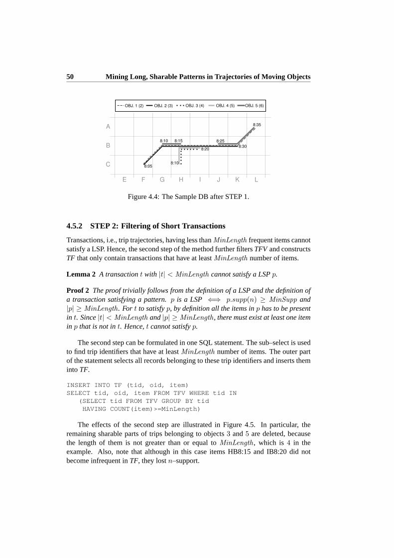
50 Mining Long, Sharable Patterns in Trajectories of Moving Objects
A
C
B
GFE KJIH L
8:158:10
8:10
8:25
8:20
8:35
8:30
OBJ. 1 (2) OBJ. 5 (6)OBJ. 4 (5)OBJ. 3 (4)OBJ. 2 (3)
8:05
Figure 4.4: The Sample DB after STEP 1.
4.5.2 STEP 2: Filtering of Short Transactions
Transactions, i.e., trip trajectories, having less thanMinLength frequent items cannotsatisfy a LSP. Hence, the second step of the method further filtersTFV and constructsTF that only contain transactions that have at leastMinLength number of items.
Lemma 2 A transactiont with |t| < MinLength cannot satisfy a LSPp.
Proof 2 The proof trivially follows from the definition of a LSP and the definition ofa transaction satisfying a pattern.p is a LSP ⇐⇒ p.supp(n) ≥ MinSupp and|p| ≥ MinLength. For t to satisfyp, by definition all the items inp has to be presentin t. Since|t| < MinLength and|p| ≥ MinLength, there must exist at least one itemin p that is not int. Hence,t cannot satisfyp.
The second step can be formulated in one SQL statement. The sub–select is usedto find trip identifiers that have at leastMinLength number of items. The outer partof the statement selects all records belonging to these trip identifiers and inserts theminto TF.
INSERT INTO TF (tid, oid, item)SELECT tid, oid, item FROM TFV WHERE tid IN
(SELECT tid FROM TFV GROUP BY tidHAVING COUNT(item)>=MinLength)
The effects of the second step are illustrated in Figure 4.5. In particular, theremaining sharable parts of trips belonging to objects3 and5 are deleted, becausethe length of them is not greater than or equal toMinLength, which is 4 in theexample. Also, note that although in this case items HB8:15 and IB8:20 did notbecome infrequent inTF, they lostn–support.
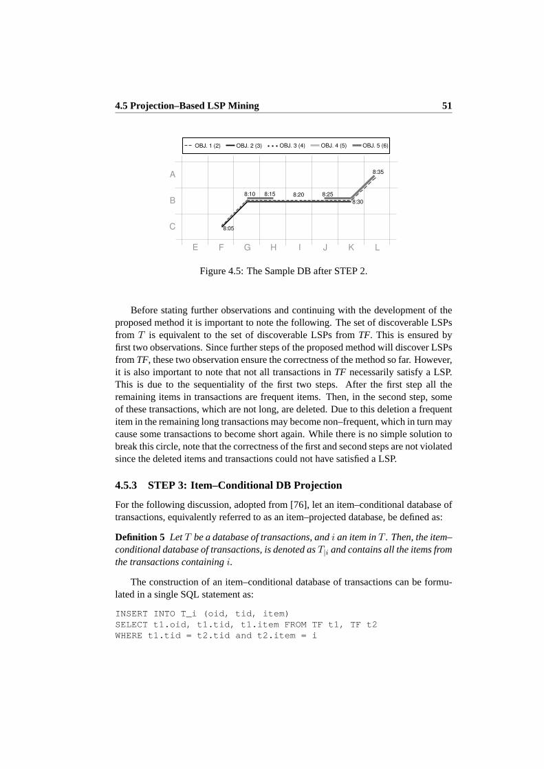
4.5 Projection–Based LSP Mining 51
A
C
B
GFE KJIH L
8:158:10 8:258:20
8:35
8:30
OBJ. 1 (2) OBJ. 5 (6)OBJ. 4 (5)OBJ. 3 (4)OBJ. 2 (3)
8:05
Figure 4.5: The Sample DB after STEP 2.
Before stating further observations and continuing with the development oftheproposed method it is important to note the following. The set of discoverableLSPsfrom T is equivalent to the set of discoverable LSPs fromTF. This is ensured byfirst two observations. Since further steps of the proposed method will discover LSPsfrom TF, these two observation ensure the correctness of the method so far. However,it is also important to note that not all transactions inTF necessarily satisfy a LSP.This is due to the sequentiality of the first two steps. After the first step all theremaining items in transactions are frequent items. Then, in the second step, someof these transactions, which are not long, are deleted. Due to this deletion afrequentitem in the remaining long transactions may become non–frequent, which in turn maycause some transactions to become short again. While there is no simple solutiontobreak this circle, note that the correctness of the first and second stepsare not violatedsince the deleted items and transactions could not have satisfied a LSP.
4.5.3 STEP 3: Item–Conditional DB Projection
For the following discussion, adopted from [76], let an item–conditional database oftransactions, equivalently referred to as an item–projected database, bedefined as:
Definition 5 LetT be a database of transactions, andi an item inT . Then, the item–conditional database of transactions, is denoted asT|i and contains all the items fromthe transactions containingi.
The construction of an item–conditional database of transactions can be formu-lated in a single SQL statement as:
INSERT INTO T_i (oid, tid, item)SELECT t1.oid, t1.tid, t1.item FROM TF t1, TF t2WHERE t1.tid = t2.tid and t2.item = i

52 Mining Long, Sharable Patterns in Trajectories of Moving Objects
Given n frequent items inT , the problem of finding CFIs can be divided inton subproblems of finding the CFIs in each of then item–projected databases [76].Using the divide–and–conquer paradigm, each of thesen subproblems can be solvedby recursively mining the item–projected databases as necessary.
4.5.4 STEP 4: Discovery of the Single Most Frequent Closed Itemset
Since i is in every transaction of the item–projected databaseT|i, and hence hasmaximumn–support, the items inT|i can be grouped in two: items that have thesamen–support asi, and items that haven–support less than that ofi. The set ofitems that have the samen–support in theT|i asi is the Single Most Frequent ClosedItemset (SMFCI) inT|i. The fourth step of the method discovers this SMFCI.
Lemma 3 Let i be an item andTF |i its corresponding item–projected database. LetA be the set of items that have the samen–support inTF |i asi. ThenA is the SMFCIin TF |i.
Proof 3 Complementary toA, let B be a set of items that haven–support less thani in TF |i. For A to be closed there should not exist an itemsetX such thatA ⊂ XandA.supp(n) = X.supp(n). This implies that there should not exist an extra itemie that is present in all transactions in whichi is present. These transactions areexactly the set of transactions that make upTF |i. The only remaining items that arenot in A and are present inTF |i are items inB. Since items inB haven–supportless than the items inA they could not be added toA to form an itemsetX suchthat A.supp(n) = X.supp(n). HenceA is a closed itemset. ThatA is the SMFCItrivially follows from the fact that the number of transaction inTF |i is A.supp(n).
The fourth step can be formulated in two SQL statements. The first statementderives then–support ofn–frequent of items inTF |i,while the second statementselects those items from thesen–frequent items that have maximumn–support.
INSERT INTO FT_i (item, i_cnt)SELECT item, COUNT(*) i_cnt FROM T_iGROUP BY item HAVING COUNT(DISTINCT oid)>=n
SELECT item FROM FT_iWHERE i_cnt = (SELECT MAX(i_cnt) FROM FT_i)
Figure 4.6 shows the effects of projectingTF based on the item FC8:05. Thenumbers in parentheses show then–support of the items inTF |FC8:05 and TF re-spectively. The SMFCI that is immediately discovered fromTF |FC8:05 is FC8:05,GB8:10, HB8:15, IB8:20, JB8:25, KB8:30. LA8:35 is the only item that is in

4.5 Projection–Based LSP Mining 53
A
C
B
GFE KJIH L
8:158:10 8:258:20
8:35
8:30
OBJ. 1 (2) OBJ. 5 (6)OBJ. 4 (5)OBJ. 3 (4)OBJ. 2 (3)
8:05
(5,5)
(5,11)
(0,8)
(5,11)(5,11)(5,5)(5,11)
Figure 4.6: Item–Conditional Sample DBTF |FC8:05and Pattern Discovery.
TF |FC8:05, but is not in the discovered SMFCI. Since further projectingTF |FC8:05
on LA8:35 yields a database of transactions where no item meets the minimumn–support criterion, the discovered SMFCI is the only CFI present inTF |FC8:05. Sincethe discovered SMFCI meets both the minimum length and an minimumn–supportcriteria it is a pattern.
Lemma 4 Given an item–projected databaseTF |i and a partitioning of items in itinto a set of most frequent itemsA, and a complementary set of itemsB, the recursiveapplication of item–projection based on items inB followed by the discovery of themost frequent closed itemsets in the respective projected databases findsall CFIs inthe item–projected databaseTF |i.
Proof 4 Given any CFIX with X.supp(n) < A.supp(n) in TF |i, X contains atleast1 item b ∈ B. If not, thenX contains only items inA, henceX.supp(n) ≥A.supp(n), which is a clear contradiction. Then by Lemma 3,X will be found asthe SMFCI inTF |i|b, sinceTF |i|b contains all, and only those transaction fromTF |i
that satisfyb.
4.5.5 STEP 5: Deletion of Unnecessary Items
The subproblems that are recursively solved by the method presented sofar are over-lapping. That is to say, viewed from a top level, a CFI that hasn items is at least oncediscovered in each of then corresponding item–projected databases. To eliminatethis redundancy, both in the mining process and the result set, observe that an itemjcan be deleted fromTF if it has the samen–support inTF |i as inTF. The intuitionbehind the observation is the following. Ifj has the samen–support inTF |i as inTF, it implies that all the transactions inTF that satisfyj are also present inTF |i.

54 Mining Long, Sharable Patterns in Trajectories of Moving Objects
A
C
B
GFE KJIH L
8:158:10 8:25
8:35
8:30
OBJ. 1 (2) OBJ. 5 (6)OBJ. 4 (5)OBJ. 3 (4)OBJ. 2 (3)
Figure 4.7: The Sample DB after STEP 5.
Thus, the set of patterns containingj, which can be discovered fromTF, can also bediscovered fromTF |i.
Lemma 5 After the construction ofTF |i, an itemj can and must be deleted fromTFif it has the samen–support inTF |i as inTF.
Proof 5 If j has the samen–support inTF as inTF |i, then the set of transactionsthat satisfyj in TF is exactly the same set of transactions that satisfyj in TF |i.Since Lemma 4 guarantees that all closed frequent itemsets will be found inTF |i,including those thatj participates in, it is needless and incorrect to construct andmineTF |j at a later point to find same CFIs thatj participates in again. Hence,jcan and must be deleted fromTF .
The fifth step can be formulated in one SQL statement. The statement deletes allitems inTF that have the samen–support inTF as inTF |i.
DELETE FROM TF WHERE TF.item IN(SELECT F.item FROM F, FT_i
WHERE F.item = FT_i.itemAND F.i_cnt = FT_i.i_cnt)
Figure 4.7 shows the effects of deleting the unnecessary items after the miningof TF |FC8:05. Since items FC:8:05 and IB8:20 have the samen–support inTF |FC8:05
as inTF, shown in Figure 4.6, they are deleted fromTF. Items remaining inTF areshown in Figure 4.7.
4.5.6 Item–Projection Ordered by Increasingn–Support
A LSPp in T , containing itemsi1 . . . ik, can be discovered from any one of the item–projected databasesT|i1 , . . . , T|ik . Steps 4 and 5 of the proposed method assure that

4.5 Projection–Based LSP Mining 55
A
C
B
GFE KJIH L
8:158:10 8:25
8:35
8:30
OBJ. 1 (2) OBJ. 5 (6)OBJ. 4 (5)OBJ. 3 (4)OBJ. 2 (3)
(8,11)
(8,8)
(8,11)(8,11)(8,11)
Figure 4.8: Item–Conditional DBTF |LA8:35 and Pattern Discovery.
p will be discovered from exactly one of these item–projected databases, but the me-thod presented so far does not specify which one. While this point is irrelevant fromthe point of view of correctness, it is crucial from the point of view of effectiveness.
To illustrate this, assume thati1.supp(n) < i2.supp(n) < . . . < ik.supp(n).If projections are performed in decreasing order of itemn–support, then, firstT|ik isconstructed, thenT|ik|ik−1
is constructed from it, and so on, all the way toT|ik|ik−1|...|i1 ,from which finallyp is discovered. If on the other hand, projections are performed inincreasing order of itemn–support, thenp is discovered from the first item–projecteddatabase that is constructed, namelyT|i1 .
Assume thatp and its qualifying(k − l + 1) (at leastl–long) sub–patterns arethe only LSPs inT . Then during the whole mining process, the total number ofprojections in the decreasing processing order isPdec = k, whereas in the increasingprocessing order the total number of projections is onlyPinc = k − l + 1. If k andlare comparable and large, thenPdec ≫ Pinc . Similar statements can be made aboutthe total size of the projected databases in both cases. Hence, item–projection shouldbe performed in increasing order of itemn-support.
4.5.7 Alternating Pattern Discovery and Deletion
Alternating steps 3, 4 and 5, all patterns can be discovered in a recursive fashion.The sequential application of these steps is referred to as aPattern Discovery andDeletion phase(PDD). Mining terminates when all items have been deleted fromTF.
Figures 4.6 and 4.7 shows the effects of the first of these PDD phases. Figures 4.8and 4.9 show the effect of the next pattern PDD phase. Since after the first PDD phaseLA8:35 has the lowestn–support inTF, namely 8, it is chosen as the next item tobase the database projection on. Figure 4.8 showTF |LA8:35 with the correspondingn–support of the items inTF |FC8:05 andTF respectively. Since all the items havethe samen–support inTF |FC8:05as LA8:35, namely 8, the closed itemsetGB8:10,

56 Mining Long, Sharable Patterns in Trajectories of Moving Objects
A
C
B
GFE KJIH L
8:158:10 8:25 8:30
OBJ. 1 (2) OBJ. 5 (6)OBJ. 4 (5)OBJ. 3 (4)OBJ. 2 (3)
Figure 4.9: The Sample DB after the Second PDD Phase.
HB8:15, JB8:25, KB8:30, LA8:35 is discovered. Since this closed itemset bothmeets the minimum length andn–support requirements it is recorded as a pattern. Inthe deletion part of this PDD phase, item LA8:35 is deleted fromTF as the only itemthat have the samen–support inTF |LA8:35 as inTF. The results of this deletion areshown on Figure 4.9.
The third and final PDD phase is implicitly shown in Figure 4.9. Since after thesecond PDD phase all the items inTF have the samen–support, the next projectionis performed on any one of the items,i, and the resulting item–projected database,TF |i, is identical to the current state ofTF, depicted on Figure 4.9. Since all the itemsin TF |i have the samen–support asi, the closed itemsetGB8:10, HB8:15, JB8:25,KB8:30 is discovered. Since this closed itemset meets both the minimum length andn–support requirements, it is recorded as a pattern. Finally, items having thesamen–support inTF |i as inTF, which in this case means all the items inTF |i, are deletedfrom TF. After this deletion part of the final PDD phase,TF becomes empty and the
A
C
B
GFE KJIH L
8:158:10 8:258:20
8:35
8:30
PAT. 1: O(1,2), S(5), L(6)
8:05
PAT. 2: O(1,5), S(8), L(5) PAT. 3: O(1,2,5), S(11), L(4)
Figure 4.10: Three Patterns in the Sample DB.
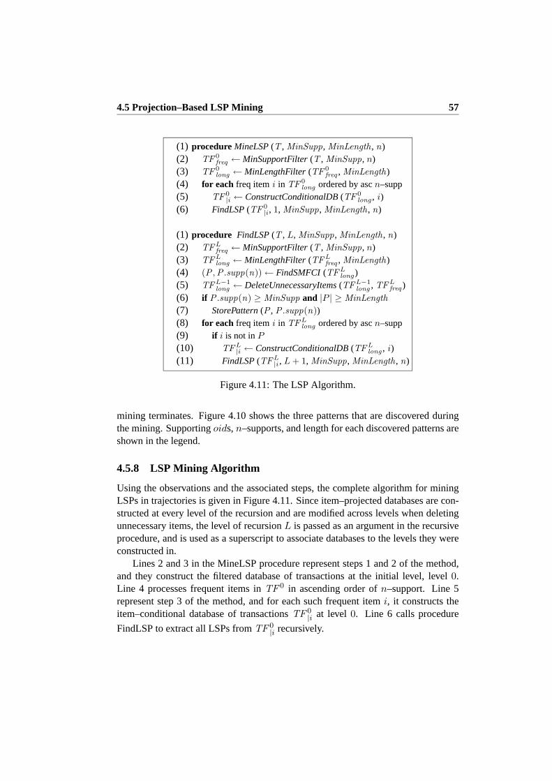
4.5 Projection–Based LSP Mining 57
(1) procedureMineLSP(T , MinSupp, MinLength, n)(2) TF 0
freq ← MinSupportFilter(T , MinSupp, n)(3) TF 0
long ← MinLengthFilter(TF 0freq , MinLength)
(4) for each freq itemi in TF 0long ordered by ascn–supp
(5) TF 0|i ← ConstructConditionalDB(TF 0
long , i )(6) FindLSP(TF 0
|i, 1, MinSupp, MinLength, n)
(1) procedure FindLSP(T , L, MinSupp, MinLength, n)(2) TFL
freq ← MinSupportFilter(T , MinSupp, n)(3) TFL
long ← MinLengthFilter(TFLfreq , MinLength)
(4) (P ,P .supp(n)) ← FindSMFCI(TFLlong )
(5) TFL−1long ← DeleteUnnecessaryItems(TFL−1
long , TFLfreq )
(6) if P .supp(n) ≥ MinSupp and |P | ≥ MinLength
(7) StorePattern(P , P .supp(n))(8) for each freq itemi in TFL
long ordered by ascn–supp(9) if i is not inP
(10) TFL|i ← ConstructConditionalDB(TFL
long , i )(11) FindLSP(TFL
|i, L + 1, MinSupp, MinLength, n)
Figure 4.11: The LSP Algorithm.
mining terminates. Figure 4.10 shows the three patterns that are discovered duringthe mining. Supportingoids,n–supports, and length for each discovered patterns areshown in the legend.
4.5.8 LSP Mining Algorithm
Using the observations and the associated steps, the complete algorithm for miningLSPs in trajectories is given in Figure 4.11. Since item–projected databases are con-structed at every level of the recursion and are modified across levels when deletingunnecessary items, the level of recursionL is passed as an argument in the recursiveprocedure, and is used as a superscript to associate databases to the levels they wereconstructed in.
Lines 2 and 3 in the MineLSP procedure represent steps 1 and 2 of the method,and they construct the filtered database of transactions at the initial level, level 0.Line 4 processes frequent items inTF 0 in ascending order ofn–support. Line 5represent step 3 of the method, and for each such frequent itemi, it constructs theitem–conditional database of transactionsTF 0
|i at level0. Line 6 calls procedure
FindLSP to extract all LSPs fromTF 0|i recursively.

58 Mining Long, Sharable Patterns in Trajectories of Moving Objects
Lines 2 and 3 in the FindLSP procedure represent steps 1 and 2 of the method,and they construct the filtered database of transactions at the current level L. Line4 represents step 4 of the method, and it finds the SMFCIP in TFL
long . Line 5represents step 5 of the method, and it deletes all items from the filtered database oftransactions of the previous level,TFL−1
long , that have the samen-support inTFL−1long
as inTFLfreq , the current level. Lines 6 and 7 check if the single most frequent closed
itemsetP meets the minimum requirements and store it accordingly. Lines 8 and 9processes frequent items inTFL
long , which are not inP , in ascending order ofn–support. Line 10 represent step 3 of the method, and for each such frequent itemi itconstructs the item–conditional database of transactionsTFL
|i at the current levelL.
Finally, line 11 recursively calls procedure FindLSP to find LSPs inTFL|i at the next
level.The structure and functionality of procedures MineLSP and FindLSP have a sig-
nificant overlap. While the two functions can be merged into one, the separation ofthe two is used to emphasize the facts that (1) DeleteUnnecessaryItems presumes theexistence of databases constructed at the previous level, and (2) FindSMFCI correctlyoperates only on an item–projected database, and hence it can only be applied at level1 and above.
Several implementation details are worth mentioning. First, DeleteUnneces-saryItems deletes items fromTFL−1
long based on then–support of items inTFLfreq ,
notTFLlong . This is important, as it was noted that MinLengthFilter decreases then–
support of items inTFLfreq , thereby possibly making an unnecessary item appear to
be necessary. Second, arguments to functions and operands in statements are logical,i.e., the functions and statements can be more efficiently implemented using previ-ously derived tables. For example, both FindSMFCI and DeleteUnnecessaryItemsare implemented using previously derivedn–support count tables not the actual tra-jectory tables. Third, simple shortcuts can significantly improve the efficiencyofthe method. For example, during the derivation ofTFL
freq , if the number of unique
frequent items inTFLfreq is less thanMinLength, no further processing is required
at that level, since none of the CFIs that can be derived fromTFLfreq are long. To
preserve clarity, these simple shortcuts are omitted from Figure 4.11.
4.6 Alternative Modelling of Trajectories and Mining of LSPs
The region–based and the road network based spatio–temporal generalization ap-proaches, presented in Section 4.3, model trajectories at a local (micro) level. Con-sequently, the method presented in Section 4.5 analyzes the trajectories at thelo-cal level and derives local (micro) patterns. Alternatively, trajectoriescan also bemodelled at the global (macro) level, whereby trips in trajectories are represented as
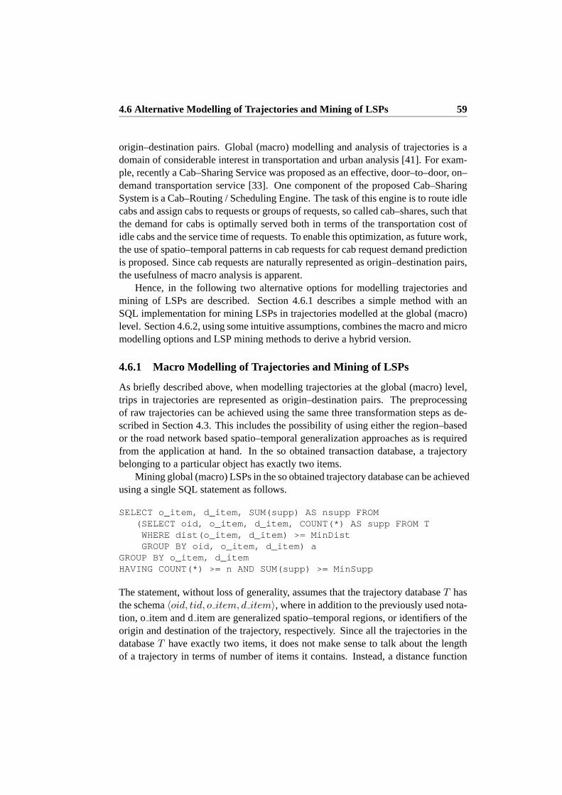
4.6 Alternative Modelling of Trajectories and Mining of LSPs 59
origin–destination pairs. Global (macro) modelling and analysis of trajectories is adomain of considerable interest in transportation and urban analysis [41]. For exam-ple, recently a Cab–Sharing Service was proposed as an effective, door–to–door, on–demand transportation service [33]. One component of the proposed Cab–SharingSystem is a Cab–Routing / Scheduling Engine. The task of this engine is to route idlecabs and assign cabs to requests or groups of requests, so called cab–shares, such thatthe demand for cabs is optimally served both in terms of the transportation cost ofidle cabs and the service time of requests. To enable this optimization, as futurework,the use of spatio–temporal patterns in cab requests for cab request demand predictionis proposed. Since cab requests are naturally represented as origin–destination pairs,the usefulness of macro analysis is apparent.
Hence, in the following two alternative options for modelling trajectories andmining of LSPs are described. Section 4.6.1 describes a simple method with anSQL implementation for mining LSPs in trajectories modelled at the global (macro)level. Section 4.6.2, using some intuitive assumptions, combines the macro and micromodelling options and LSP mining methods to derive a hybrid version.
4.6.1 Macro Modelling of Trajectories and Mining of LSPs
As briefly described above, when modelling trajectories at the global (macro) level,trips in trajectories are represented as origin–destination pairs. The preprocessingof raw trajectories can be achieved using the same three transformation steps as de-scribed in Section 4.3. This includes the possibility of using either the region–basedor the road network based spatio–temporal generalization approaches as is requiredfrom the application at hand. In the so obtained transaction database, a trajectorybelonging to a particular object has exactly two items.
Mining global (macro) LSPs in the so obtained trajectory database can be achievedusing a single SQL statement as follows.
SELECT o_item, d_item, SUM(supp) AS nsupp FROM(SELECT oid, o_item, d_item, COUNT(*) AS supp FROM T
WHERE dist(o_item, d_item) >= MinDistGROUP BY oid, o_item, d_item) a
GROUP BY o_item, d_itemHAVING COUNT(*) >= n AND SUM(supp) >= MinSupp
The statement, without loss of generality, assumes that the trajectory databaseT hasthe schema〈oid, tid, o item, d item〉, where in addition to the previously used nota-tion, o item and ditem are generalized spatio–temporal regions, or identifiers of theorigin and destination of the trajectory, respectively. Since all the trajectories in thedatabaseT have exactly two items, it does not make sense to talk about the lengthof a trajectory in terms of number of items it contains. Instead, a distance function

60 Mining Long, Sharable Patterns in Trajectories of Moving Objects
A
C
B
GF KJIH L
8:00
8:158:05 8:10 8:20 8:25
8:30
8:00 8:30
Figure 4.12: Loss of Local (Micro) LSP.
dist() between two locations or items can be defined, and patterns can be evaluatedagainst aMinDist criterion. The inner select statement calculates the supports forobject–specific origin–destination item combinations that satisfy theMinDist crite-rion. The outer select statement aggregates the results of the inner selectstatement,and identifies origin–destination item combinations that meet then–support criterion,i.e., global (macro) LSPs, and calculates their correspondingn–supports.
4.6.2 Hybrid Modelling of Trajectories and Mining of LSPs
The proposed global (macro) modelling approach of trajectories, the global (macro)LSP mining method and the SQL implementation given for it are likely to be very ef-ficient due to the indexing and aggregation support provided by RDBMSs. However,the discovered global (macro) LSPs, will have very little relation to each other. Forexample, a set of individual global (macro) LSPs, considering the underlying roadnetwork, might give rise to local (micro) LSPs that do not exist in the macro model,but have a support that is equal to the sum of then-supports of the individual patterns.As an illustrative example consider the road network represented by the solid blacklines in Figure 4.12. Assume that for a particular setting of the parameters, theglobal(macro) LSP mining method finds two global (macro) LSPs,FA8:00, LA8:30 andFC8:00, LC8:30, with n–supports 10 for each. Assuming that the spatial regionsFA, LA, FC, and LC cover the only four cities in the area, and hence trajectoriesonly start and finish in these regions, the global (macro) LSP mining method willnotdiscover the local (micro) LSPGB8:05, HB8:10, IB8:15, JB8:20, KB8:25 withn–support 20.
To overcome this deficiency of the global (macro) LSP mining method, the global(macro) and the local (micro) modelling approaches and LSP mining methods can becombined into a hybrid modelling and LSP mining method as follows. First, performglobal (macro) LSP mining on the spatio–temporally generalized input trajectories.

4.6 Alternative Modelling of Trajectories and Mining of LSPs 61
(1) procedureHybridMineLSP(Traj I , MinDist , MinSupp, MinLength, n)(2) TrajG ← STGeneralize(Traj I )(3) LSPmacro ← MacroMineLSP(TrajG, MinDist , MinSupp, n)(4) TrajA ← ApproximateTraj(LSPmacro)(5) TrajGA ← STGeneralize(TrajA)(6) LSPmicro ← MineLSP(TrajGA, MinLength, MinSupp = 1, n = 1)
Figure 4.13: The Hybrid LSP Mining Method.
Then, using the global (macro) LSPs and the underlying road network,approximatetrajectories for the global (macro) LSPs, i.e., find shortest paths betweenorigin–destination pairs. Then, spatio–temporally generalize the approximated trajectoriesand mine local (micro) LSPs in them, taking into account the global (macro)n–supports of the approximated trajectories. Taking into accountn–supports of theapproximated trajectories can either be achieved by slightly modifying the local(mi-cro) LSP mining method in Section 4.5, or simply the original version of it can becalled with parametersn = 1 andMinSupp = 1. The latter is necessary and suffi-cient to ensure that (1) the approximated trajectories belonging to the global(macro)LSPs are found as local (micro) LSPs as well, and (2) the local (micro) LSPs foundmeet the originaln–support criterion. Note that the spatio–temporal generalizationof the input and approximated trajectories can either be regions–based orroad net-work based. Figure 4.13 gives the pseudo code of the hybrid LSP mining method, asdescribed above.
While the hybrid LSP mining method is likely to reduce the number of input tra-jectories to the local (micro) LSP mining method called internally, thereby achievinga significant speed–up in running time, it does not findall the local (micro) LSPs.As an example consider the trajectories in Figure 4.12. IfMinSupp = 20, then thehybrid LSP mining method will not find any patterns in the global (macro) LSP min-ing phase, and consequently will not find any local (micro) LSPs, even though thelocal (micro) LSPGB8:05, HB8:10, IB8:15, JB8:20, KB8:25 has ann–support of20. Similarly, it can be argued that the hybrid LSP mining method will not find anyLSPs in the example trajectory database in Section 4.3.2, for the parameters used inthe running example in Section 4.5. However, as the spatio–temporal generalizationgranularity used in the mining is decreased the chances not identifying global (macro)LSPs that give rise to local (micro) LSPs is decreased. In summary, the hybrid LSPmining method is likely an effective alternative that provides lossy and approximateresults when compared to the local (micro) LSP mining method.
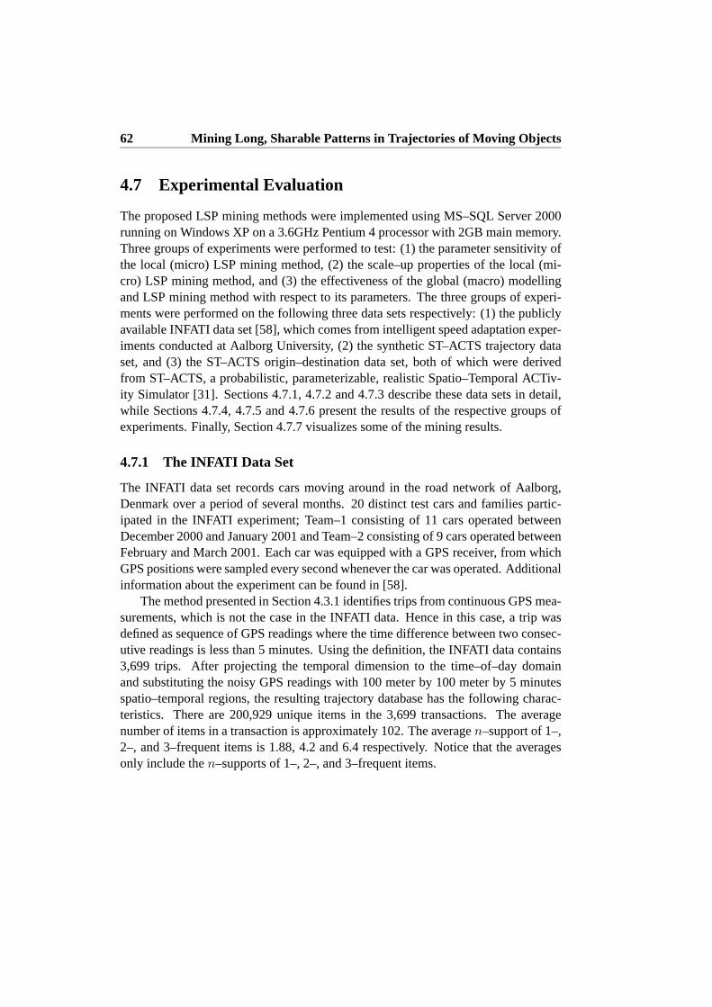
62 Mining Long, Sharable Patterns in Trajectories of Moving Objects
4.7 Experimental Evaluation
The proposed LSP mining methods were implemented using MS–SQL Server 2000running on Windows XP on a 3.6GHz Pentium 4 processor with 2GB main memory.Three groups of experiments were performed to test: (1) the parameter sensitivity ofthe local (micro) LSP mining method, (2) the scale–up properties of the local (mi-cro) LSP mining method, and (3) the effectiveness of the global (macro) modellingand LSP mining method with respect to its parameters. The three groups of experi-ments were performed on the following three data sets respectively: (1) thepubliclyavailable INFATI data set [58], which comes from intelligent speed adaptation exper-iments conducted at Aalborg University, (2) the synthetic ST–ACTS trajectory dataset, and (3) the ST–ACTS origin–destination data set, both of which were derivedfrom ST–ACTS, a probabilistic, parameterizable, realistic Spatio–TemporalACTiv-ity Simulator [31]. Sections 4.7.1, 4.7.2 and 4.7.3 describe these data sets in detail,while Sections 4.7.4, 4.7.5 and 4.7.6 present the results of the respective groups ofexperiments. Finally, Section 4.7.7 visualizes some of the mining results.
4.7.1 The INFATI Data Set
The INFATI data set records cars moving around in the road network ofAalborg,Denmark over a period of several months. 20 distinct test cars and familiespartic-ipated in the INFATI experiment; Team–1 consisting of 11 cars operated betweenDecember 2000 and January 2001 and Team–2 consisting of 9 cars operated betweenFebruary and March 2001. Each car was equipped with a GPS receiver, from whichGPS positions were sampled every second whenever the car was operated. Additionalinformation about the experiment can be found in [58].
The method presented in Section 4.3.1 identifies trips from continuous GPS mea-surements, which is not the case in the INFATI data. Hence in this case, a tripwasdefined as sequence of GPS readings where the time difference betweentwo consec-utive readings is less than 5 minutes. Using the definition, the INFATI data contains3,699 trips. After projecting the temporal dimension to the time–of–day domainand substituting the noisy GPS readings with 100 meter by 100 meter by 5 minutesspatio–temporal regions, the resulting trajectory database has the followingcharac-teristics. There are 200,929 unique items in the 3,699 transactions. The averagenumber of items in a transaction is approximately 102. The averagen–support of 1–,2–, and 3–frequent items is 1.88, 4.2 and 6.4 respectively. Notice that the averagesonly include then–supports of 1–, 2–, and 3–frequent items.

4.7 Experimental Evaluation 63
4.7.2 The ST–ACTS Trajectory Data Set
The ST–ACTS trajectory data set is based on the output of ST–ACTS, a probabilis-tic, parameterizable, realistic Spatio–Temporal ACTivity Simulator [31]. Based ona number of real world data sources and a set of principles that try to model thesocial and some of thephysicalaspects of mobility, ST–ACTS simulates realisticspatio–temporal activity sequences of approximately 600,000 individuals inthe cityof Copenhagen, Denmark. Since the aim of ST–ACTS is to simulate realistic spatio–temporal activities of individuals that contain patterns, rather than to simulate detailedmovements of individuals, the output of the ST–ACTS for each simulated individualis a sequence of timestamped locations and activities. Two consecutive locations insuch a sequence can be seen as the origin and the destination of a trip’s trajectory.To obtain a realistic approximation for the missing part of the trajectories, usingtheunderlying road network, segment–based shortest path calculations were performedbetween the origin–destination pairs of the trips. The so obtained trip trajectories areanalogous in form and semantics to the trajectories that can be obtained usingtheroad network based spatio–temporal generalization approach as explained in Section4.3.1.
For the period of three working days, spatio–temporal activities of 5,000 individ-uals were simulated, resulting in a total of 64,144 trips. Using segment–based routingbetween origin–destination pairs, an average trip is 1,850 meters long with a standarddeviation of 1,937 meters, and is made up of 28 road segments with a standard devia-tion of 27 road segments. An average road segment is 66 meters long with a standarddeviation of 64 meters. After projecting the temporal dimension to the time–of–daydomain and using the road segments as spatial–, and a 15–minute interval as tem-poral, generalization units, the resulting trajectory database has the following char-acteristics. There are 330,940 unique items in the 64,144 transactions. The averagenumber of items in a transactions is approximately 28. To test the scale–up proper-ties of the proposed method, varying sized subsets of the ST–ACTS trajectory dataset were constructed. Figure 4.14 summarizes the characteristics of thesesubsets interms of the number (Figure 4.14(a)) andn–support (Figure 4.14(b)) ofn–frequentitems. While not shown in Figure 4.14, the number of trajectories linearly scaleswiththe number of objects in the data sets between 6,601 trajectories for 500 objects and64,144 trajectories for 5,000 objects. Similar linear relationships exist between thenumber of objects and the averagen–support ofn–frequent items, Figure 4.14(b).The logarithmic like relationships between the number of objects and the number ofn–frequent items is due to the fact that the increasing number of trajectories traverse,and maken–frequent, an increasing fraction of road segments of the total road net-work, see Figure 4.14(a). In other words, the number ofn–frequent items naturallysaturates as the density of the trajectories increases.

64 Mining Long, Sharable Patterns in Trajectories of Moving Objects
500 1000 1500 2000 2500 3000 3500 4000 4500 50000
0.5
1
1.5
2
2.5
3
3.5x 10
5
number of objects
coun
t of n
−fr
eque
nt it
ems
1−freq
2−freq
3−freq
4−freq
5−freq
(a) Number ofn–Frequent Items.
500 1000 1500 2000 2500 3000 3500 4000 4500 50000
2
4
6
8
10
12
14
number of objects
aver
age
n−su
ppor
t of n
−fr
eque
nt it
ems
1−freq
2−freq
3−freq
4−freq
5−freq
(b) Averagen–Support ofn–Frequent Items.
Figure 4.14: Data Characteristics of Varying Sized Subsets of the ST–ACTS Trajec-tory Data Set.
4.7.3 The ST–ACTS Origin–Destination Data Set
The ST–ACTS origin–destination data set, similarly to the ST–ACTS trajectory dataset, is also based on the output of ST–ACTS. However, it includes the spatio–temporalactivities of 50,000 individuals for a period of three working days, resulting in a totalof 835,806 trips. The average Euclidean distance between the origins anddestina-tions of the trips is 1,199 meters with a standard deviation of 1.555 meters. Afterprojecting the temporal dimension to the time–of–day domain and substituting theorigins and destinations of trips with 100 meter by 100 meter by 15–minute spatio–temporal regions, the resulting trajectory database has the following characteristics.There are 139,480 unique items in the 1,671,612 transactions. The number ofitemsin every transactions is exactly 2, which correspond to an origin and a destinationspatio–temporal region. The averagen–support (and count) of 1–, 2–, 3–, and 4–frequent items is 1.12 (1,497,871), 2.14 (152,255), 3.24 (17,267), and 4.09 (3854)respectively. Notice that the averages only include then–supports of 1–, 2–, 3–, and4–frequent items.
4.7.4 Sensitivity Experiments forMinSupp and MinLength Parameters
The first group of experiments was performed to test the sensitivity of local (micro)LSP mining method with respect to theMinSupp andMinLength parameters, andwas using the INFATI data set as input. Two sets of experiments were performed,each varying one of the two parameters of the algorithm,MinSupp andMinLength.The performance of the algorithm was measured in terms of processing time andworking space required, where the working space required by the algorithm was ap-proximated by the sum of the rows in the projected tables that were constructed by
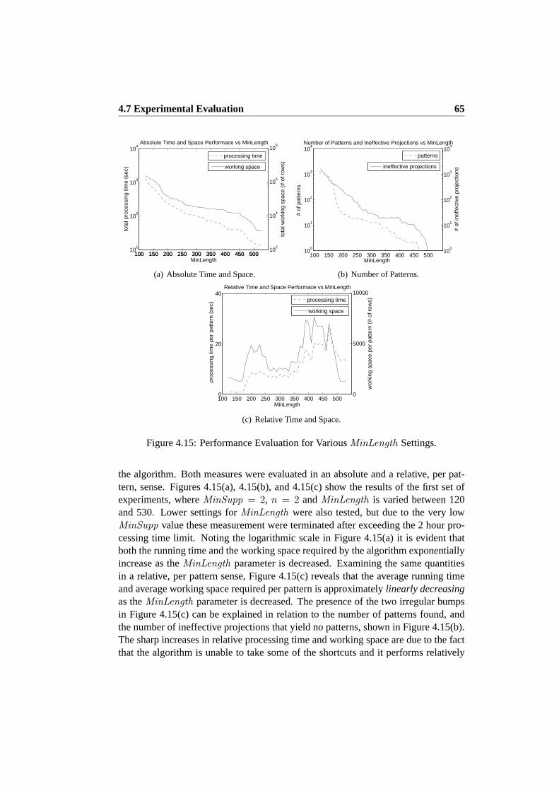
4.7 Experimental Evaluation 65
100 150 200 250 300 350 400 450 50010
1
102
103
104
MinLength
tota
l pro
cess
ing
time
(sec
)
Absolute Time and Space Performace vs MinLength
100 150 200 250 300 350 400 450 50010
2
104
106
108
tota
l wor
king
spa
ce (
# of
row
s)working space
processing time
(a) Absolute Time and Space.
100
101
102
103
104
Number of Patterns and Ineffective Projections vs MinLength
# of
pat
tern
s
MinLength100 150 200 250 300 350 400 450 500
100
101
102
103
104
# of
inef
fect
ive
proj
ectio
ns
ineffective projections
patterns
(b) Number of Patterns.
100 150 200 250 300 350 400 450 5000
20
40Relative Time and Space Performace vs MinLength
proc
essi
ng ti
me
per
patte
rn (
sec)
MinLength
0
5000
10000
wor
king
spa
ce p
er p
atte
rn (
# of
row
s)processing time
working space
(c) Relative Time and Space.
Figure 4.15: Performance Evaluation for VariousMinLength Settings.
the algorithm. Both measures were evaluated in an absolute and a relative, per pat-tern, sense. Figures 4.15(a), 4.15(b), and 4.15(c) show the results of the first set ofexperiments, whereMinSupp = 2, n = 2 andMinLength is varied between 120and 530. Lower settings forMinLength were also tested, but due to the very lowMinSupp value these measurement were terminated after exceeding the 2 hour pro-cessing time limit. Noting the logarithmic scale in Figure 4.15(a) it is evident thatboth the running time and the working space required by the algorithm exponentiallyincrease as theMinLength parameter is decreased. Examining the same quantitiesin a relative, per pattern sense, Figure 4.15(c) reveals that the average running timeand average working space required per pattern is approximatelylinearly decreasingas theMinLength parameter is decreased. The presence of the two irregular bumpsin Figure 4.15(c) can be explained in relation to the number of patterns found, andthe number of ineffective projections that yield no patterns, shown in Figure 4.15(b).The sharp increases in relative processing time and working space are due to the factthat the algorithm is unable to take some of the shortcuts and it performs relatively
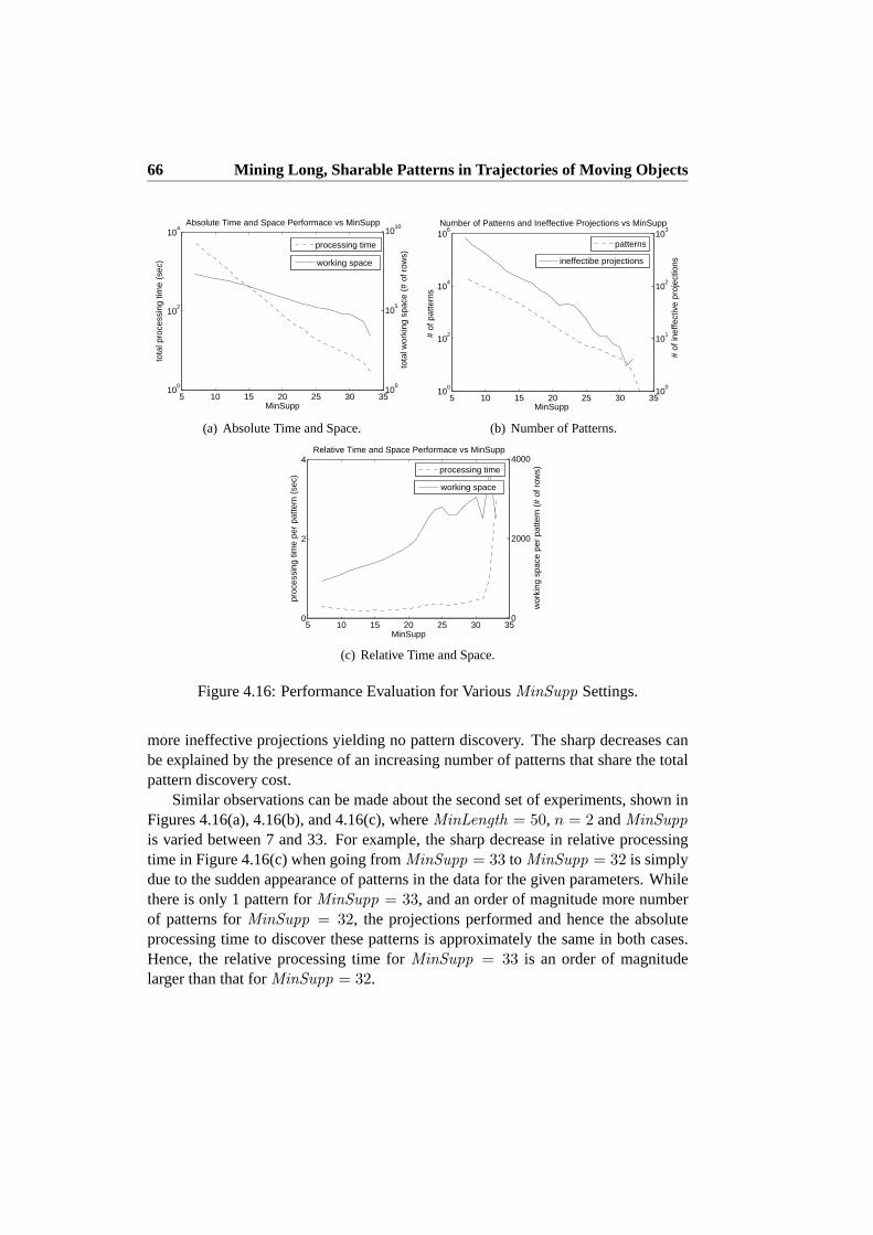
66 Mining Long, Sharable Patterns in Trajectories of Moving Objects
5 10 15 20 25 30 3510
0
102
104
Absolute Time and Space Performace vs MinSupp
tota
l pro
cess
ing
time
(sec
)
MinSupp
100
105
1010
tota
l wor
king
spa
ce (
# of
row
s)
processing time
working space
(a) Absolute Time and Space.
100
102
104
106
Number of Patterns and Ineffective Projections vs MinSupp
# of
pat
tern
s
MinSupp5 10 15 20 25 30 35
100
101
102
103
# of
inef
fect
ive
proj
ectio
nsineffectibe projections
patterns
(b) Number of Patterns.
5 10 15 20 25 30 350
2
4Relative Time and Space Performace vs MinSupp
proc
essi
ng ti
me
per
patte
rn (
sec)
MinSupp
0
2000
4000
wor
king
spa
ce p
er p
atte
rn (
# of
row
s)processing time
working space
(c) Relative Time and Space.
Figure 4.16: Performance Evaluation for VariousMinSupp Settings.
more ineffective projections yielding no pattern discovery. The sharp decreases canbe explained by the presence of an increasing number of patterns that share the totalpattern discovery cost.
Similar observations can be made about the second set of experiments, shown inFigures 4.16(a), 4.16(b), and 4.16(c), whereMinLength = 50, n = 2 andMinSupp
is varied between 7 and 33. For example, the sharp decrease in relative processingtime in Figure 4.16(c) when going fromMinSupp = 33 to MinSupp = 32 is simplydue to the sudden appearance of patterns in the data for the given parameters. Whilethere is only 1 pattern forMinSupp = 33, and an order of magnitude more numberof patterns forMinSupp = 32, the projections performed and hence the absoluteprocessing time to discover these patterns is approximately the same in both cases.Hence, the relative processing time forMinSupp = 33 is an order of magnitudelarger than that forMinSupp = 32.

4.7 Experimental Evaluation 67
1000 1500 2000 2500 3000 3500 400010
1
102
103
104
105Absolute Time and Space Performance vs. # Objects
tota
l pro
cess
ing
time
(sec
)
number of objects
1000 1500 2000 2500 3000 3500 400010
4
105
106
107
tota
l wor
king
spa
ce (
# of
row
s)
processing time
working space
(a) Absolute Time and Space.
1000 1500 2000 2500 3000 3500 400010
0
105
Number of Patterns and Ineffective Projections vs. # Objects
# of
pat
tern
s
number of objects
1000 1500 2000 2500 3000 3500 400010
0
105
# of
inef
fect
ive
proj
ectio
ns
patterns
ineffective projections
(b) Number of Patterns.
1000 1500 2000 2500 3000 3500 40000
10
20Relative Time and Space Performace vs. # Objects
proc
essi
ng ti
me
per
patte
rn (
sec)
number of objects
1000 1500 2000 2500 3000 3500 40000
10K
wor
king
spa
ce p
er p
atte
rn (
# of
row
s)
processing time
working space
(c) Relative Time and Space.
Figure 4.17: Performance Evaluation for Various Sized Data Sets, i.e., Number ofObjects.
4.7.5 Scale–up Experiments for Various Input Data Sizes
The second group of experiments was performed to test the scale–up properties ofthe local (micro) LSP mining method for varying size input data, and was performedusing the ST–ACTS trajectory data set. For this group of experiments the algorithm’sparameters were kept constant atn = 4, MinSupp = 8 andMinLength = 25. Inother words, the patterns sought for were sub–trajectories with a minimum length of25 road segments that were supported by at least 4 objects on average at least twotimes per object. The evaluation measures used in the experiments were the sameas in the sensitivity experiments described in Section 4.7.4. Figure 4.17 showstheresults of this group of experiments. The results can be summarized as follows. Asthe number of objects increases linearly, i.e. the density of the trajectories increaseslinearly, the number of patterns increases sub–exponentially, see Figure4.17(b). Thisnaturally leads to a sub–exponential increase in absolute running time (Figure 4.17(a)

68 Mining Long, Sharable Patterns in Trajectories of Moving Objects
left) and working space (Figure 4.17(a) right). However, the examinationof the samequantities in a relative, per pattern sense, see Figure 4.17(c), reveals that the averagerunning time required per pattern gradually decreases to a close to constant value ofa few seconds as the density of the trajectories increases. This is due to thefact thatas the density of the trajectories is increasing, the number of ineffective projectionsrelative to the number of patterns, i.e., the gap between the two, is decreasing, seeFigure 4.17(c). Similar observations can be made about the average working spacerequired per pattern. In summary, the scale–up experiments show that boththe run-ning time of, and working space required by the local (macro) LSP mining methodscale sub–exponentially with the input data size and linearly with the output datasize.
2 4 6 8 10
0.5
1
1.5
2
2.5
x 104
n
# of
pat
tern
s
grid size = 100mgrid size = 250mgrid size = 500mgrid size = 750mgrid size = 1000m
(a) Varyingn.
5 10 15 20
0.5
1
1.5
2
2.5
x 104
MinSupp
# of
pat
tern
s
grid size = 100mgrid size = 250mgrid size = 500mgrid size = 750mgrid size = 1000m
(b) VaryingMinSupp.
1000 2000 3000 4000 5000
1
2
3
4
5
x 104
MinDist
# of
pat
tern
s
grid size = 100mgrid size = 250mgrid size = 500mgrid size = 750mgrid size = 1000m
(c) VaryingMinDist .
Figure 4.18: Number of Global (Macro) LSPs for Varying Spatio–Temporal Granu-larities and Parameter Settings.

4.7 Experimental Evaluation 69
45005000
55006000
6500
6.1
6.2
6.3
6.4
x 104
0
1
2
3
4
x 104
X−coor (100m)
Trajectories of 20 moving objects in INFATI
Y−coor (100m)
Tim
e (5
min
)
(a) Moving Object Trajectories.
50005200
54005600
58006000
6.2
6.25
6.3
6.35
6.4
x 104
800
1000
1200
1400
1600
1800
2000
X−coor (100m)
28 long, common patterns in real−world trajectories
Y−coor (100m)
Tim
e−of
−da
y (5
min
)
(b) 28 Discovered LSPs.
Figure 4.19: LSP Discovery Results in the INFATI Data Set.
4.7.6 Global (Macro) Modelling and LSP Mining Experiments
The third group of experiments was performed to test the effectiveness of the global(macro) modelling and LSP mining method, as presented in Section 4.6.1. The ex-periments were performed for varying spatio–temporal generalization granularitiesfor varying n, MinSupp andMinDist parameters, and were using the ST–ACTSorigin–destination data set. Figure 4.18 shows the results of this group of experi-ments. The trends in the results are as expected. As the values for the parametersn, MinSupp andMinDist increases the number of global (macro) LSPs decreases,shown in Figures 4.18(a), 4.18(b), and 4.18(c), respectively. Similarly, all experi-ments show that as the spatio–temporal regions become coarser the number of pat-terns found increases. Perhaps more notable is the fact that for the rather large dataset, with appropriate indexing the running time of the global (macro) LSP miningmethod is independent of the parameters and is under 2 seconds.
4.7.7 Visualization of Patterns
To see the benefits of mining LSPs, the mining results of two mining tasks are visual-ized in the following. Figure 4.19 presents the mining results of finding local (micro)patterns in the region–based spatio–temporally generalized INFATI data using theLSP algorithm from Section 4.5. Figure 4.19(a) shows a 50–fold down–sampled ver-sion of the trajectories of the 20 moving objects in the INFATI data set. While someregularities are apparent in it to the human eye, to find LSPs in it seems like a daunt-ing task. Figure 4.19(b) shows 28 LSPs in it that are at least 200 long, sharable for atleast 2 distinct objects, and have a support of at least 2.
Figure 4.20 presents the mining results of finding local (micro) patterns in theroad network based spatio–temporally generalized ST–ACTS origin–destination data
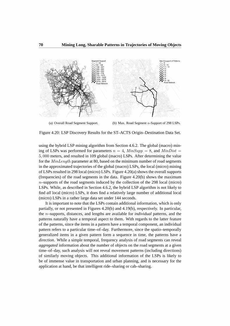
70 Mining Long, Sharable Patterns in Trajectories of Moving Objects
Road Network
Segment Support1 - 5455 - 138139 - 247248 - 383384 - 555556 - 778779 - 10731074 - 15291530 - 22782279 - 3610
(a) Overall Road Segment Support.
Road Network
Max N-support of Patterns89 - 1011 - 1213141516171819 - 30
(b) Max. Road Segmentn-Support of 298 LSPs.
Figure 4.20: LSP Discovery Results for the ST–ACTS Origin–Destination Data Set.
using the hybrid LSP mining algorithm from Section 4.6.2. The global (macro) min-ing of LSPs was performed for parametersn = 4, MinSupp = 8, andMinDist =5, 000 meters, and resulted in 109 global (macro) LSPs. After determining the valuefor theMinLength parameter at 80, based on the minimum number of road segmentsin the approximated trajectories of the global (macro) LSPs, the local (micro)miningof LSPs resulted in 298 local (micro) LSPs. Figure 4.20(a) shows the overall supports(frequencies) of the road segments in the data. Figure 4.20(b) shows themaximumn–supports of the road segments induced by the collection of the 298 local (micro)LSPs. While, as described in Section 4.6.2, the hybrid LSP algorithm is not likely tofind all local (micro) LSPs, it does find a relatively large number of additional local(micro) LSPs in a rather large data set under 144 seconds.
It is important to note that the LSPs contain additional information, which is onlypartially, or not presented in Figures 4.20(b) and 4.19(b), respectively. In particular,then–supports, distances, and lengths are available forindividual patterns, and thepatterns naturally have a temporal aspect to them. With regards to the latter featureof the patterns, since the items in a pattern have a temporal component, an individualpattern refers to a particular time–of–day. Furthermore, since the spatio–temporallygeneralized items in a given pattern form a sequence in time, the patterns haveadirection. While a simple temporal, frequency analysis of road segments can revealaggregatedinformation about the number of objects on the road segments at a giventime–of–day, such analysis will not reveal movement patterns (including directions)of similarly moving objects. This additional information of the LSPs is likely tobe of immense value in transportation and urban planning, and is necessaryfor theapplication at hand, be that intelligent ride–sharing or cab–sharing.

4.8 Conclusions and Future Work 71
4.7.8 Summary of Experimental Results
In conclusion, the experimental evaluations can be summarized as follows. First, thesensitivity experiments show that the LSP mining method, presented in Section 4.5, iseffective and is robust to changes in the user–defined parameter settings,MinLength
andMinSupp, and is a useful analysis tool for finding LSPs in moving object tra-jectories. Second, the scale–up experiments show that while the absolute runningtime and space required to find LSPs scales exponentially with the input data size,this is mainly due to the fact that the number of LSPs that are present in the inputdata, i.e., the output data size, also scales exponentially with the input data size. Thescale–up experiments also demonstrate that the relative, per pattern, performance ofthe LSP mining method gradually decreases to a constant value as the input data sizeis increased. This later property of the LSP method is due to the fact that as the in-put size is increased, i.e., the density of the trajectories is increased, the effects oftheMinLength andMinSupp pruning criteria become more dominant and relativelyless and less ineffective projections are performed. Third, the experiments relating toglobal (macro) modelling and LSP mining, show that this modelling option and LSPmining method is extremely effective on large data sets, and is rather insensitive tothe user–defined parameter settings,n, MinDist andMinSupp. Finally, brief exper-iments show that the hybrid modelling and LSP mining method, while missing somelocal (micro) LSPs due to the partial global (macro) modelling, is able to find local(micro) LSPs in large data sets effectively.
4.8 Conclusions and Future Work
The herein presented work, for the first time, considers the problem of mining LSPsin trajectories and transforms it to a framework similar to that used in frequentitem-set mining. The transformation allows both region–based and road networkbasedspatio–temporal generalizations of trajectories. Two methods and their simple SQL–implementations are presented for mining either local (micro) or global (macro)LSPsin such spatio–temporally generalized trajectories. In an attempt to speed up the local(micro) LSP mining method, the two methods are combined to a hybrid LSP miningmethod, which is able to rapidly find most of the local (micro) LSPs. The effective-ness of the different LSP methods is demonstrated through extensive experiments onboth a real world data set, and a number of large–scale, synthetic data sets.
Future work is planed along several directions. First, as discussed, thehybrid LSPmethod, while is able to achieve significant speed–up compared to the local (micro)LSP mining method, it does not find all the local (micro) LSPs in the trajectories.Hence future work will consider to quantify (1) the speed–up of the hybrid LSPmethod, and (2) the fraction of the local (micro) LSPs found by the hybrid LSP

72 Mining Long, Sharable Patterns in Trajectories of Moving Objects
method. Second, the large number of patterns discovered are difficult to analyze. Toreduce this number, future work will consider the mining of a compressed patterns intrajectories [101]. Finally, future work will consider the partitioning of trajectoriesusing index structures designed for trajectories, like in [55], to allow the distributed /parallel mining of LSPs.
Chapter 5
Cab–Sharing: An Effective,Door–To–Door, On–DemandTransportation Service
City transportation is an increasing problem. Public transportation is costeffective,but do not provide doortodoor transportation; This makes the far more expensivecabs attractive and scarce. This paper proposes a location–based Cab–Sharing Ser-vice (CSS), which reduces cab fare costs and effectively utilizes available cabs. TheCSS accepts cab requests from mobile devices in the form of origin–destination pairs.Then it automatically groups closeby requests to minimize the cost, utilize cab space,and service cab requests in a timely manner. Simulation–based experiments showthat the CSS can group cab requests in a way that effectively utilizes resources andachieves significant savings, making cab–sharing a new, promising mode of trans-portation.
5.1 Introduction
Transportation in larger cities, including parking, is an ever increasing problem thataffects the environment, the economy, and last but not least our lives. Traffic jamsand the hustle of parking take up a significant portion of our daily lives andcausemajor headaches. Solving the problem by extending the road network is a costlyand non–scalable solution. A more feasible solution to the problem is to reducethenumber of cars on the existing road network. To achieve this, collective / publictransportation tries to satisfy the general transportation needs of larger groups in a
73

74 Cab–Sharing: An Effective, On–Demand Transportation Service
cost–effective manner. While being cost–effective, the services offered by publictransportation often (1) do not meet the exact, door–to–door transportation needsof individuals, (2) require multiple transfers and detours that significantlylengthentravel times, and (3) are limited in off–peak hours. For these reasons, thefar moreexpensive service offered by cabs / taxis, which meet the exact transportation needs ofindividuals and also eliminates the problem of parking, are in great demand.To bettersatisfy this demand, this paper presents an LBS that makes use of simple technologiesand tools to offer a new cost– and resource–effective, door–to–door transportationmeans, namelycab–sharing.
Collective transportation is not a new concept. It is encouraged and subsidizedby transportation authorities all over the world. The optimization of collective trans-portation has also been considered. For an extensive list of researchpapers in thisarea, the reader is referred to [92]. Two papers, however, are worth highlighting.First, in [32], where the idea of the present research originates from, inan off–linefashion, long, shareable patterns are sought in historical trajectories of moving ob-jects to aid an intelligent ride–sharing application. Second, in [17] an almost “per-sonalized” transportation system is proposed that alters the fixed–line buss service toinclude variable itineraries and timetables. In comparison, the herein proposed CSStreats the optimization of collective transportation as a truly online process, and altersthe inherently routeless transportation service offered by cabs.
5.2 Problem Statement
Let R2 denote the 2-dimensional Euclidean space, and letT ≡ N
+ denote the totallyordered time domain. LetR = r1, . . . , rn be a set ofcab requests, such thatri = 〈tr, lo, ld, te〉, wheretr ∈ T is therequest timeof the cab request,lo ∈ R
2 andld ∈ R
2 are theorigin anddestination locationsof the cab request, andte ≥ tr ∈ T
is theexpiration timeof the cab request, i.e., the latest time by which the cab requestmust be serviced. A cab requestri =< tr, lo, ld, te > is valid at timet if tr ≤ t ≤ te.Let ∆t = te − tr be called thewait timeof the cab request. Let acab–shares ⊆ Rbe a subset of the cab requests. A cab–share is valid at timet if all cab requestsin s are valid at timet. Let |s| denote the number of cab request in the cab–share.Let d(l1, l2) be a distance measure between two locationsl1 andl2. Let m(s, d(., .))be a method that constructs a valid and optimal pick–up and drop–off sequence ofrequests for a cab–shares and assigns a unique distance to this sequence based ond(., .). Let thesavingsp for a cab requestri ∈ s bep(ri, s) = 1− m(s,d(.,.))/|s|
m(ri,d(.,.)) . Then,thecab–sharing problemis to find a disjoint partitioningS = s1 ⊎ s2 ⊎ . . . of R,such that∀sj ∈ S, sj is valid, |sj | ≤ K, and the expression
∑
sj∈S
∑
ri∈sjp(ri, sj)
is maximized.

5.3 Cab–Sharing Service 75
Premium SMSCab-Sharing
Service
GeocodingService
Cab-SharingEngine
User Accounts DB
Cab-Scheduling /Cab-Routing
Engine
Text Msg:To: 1234From Addr.To Addr.
[From/To addr.]
[From/To coord.]
SMS: cab request
SMS: fare info[cost, schedule]
Check fu
nds
[uid
, cost]F
unds O
K
[From/To coord., uid]
Cab-share info[uids, cost, shares]
Cab-s
hare
info
Cab-f
are
info
[cabid
, schedule
]
Figure 5.1: Cab–Sharing Service Components and Process.
5.3 Cab–Sharing Service
The Cab–Sharing Service (CSS) is depicted in Figure 5.1. Before using the CSS, auser signs up with the CSS and creates a prepaid user account to pay forthe service.A registered user sends a cab request in the form of an origin–destination pair andan optional validity period of the request. In case no validity period is specified, thecab request is assumed to be valid from the time it is received until some defaulttime limit has been reached. The requests are submitted via a mobile device bysending two address lines to a premium SMS service, called Premium Cab–SharingService. A more user–friendly specification of requests could include GPS–basedlocalization of origins and/or the ability of users selecting origins and/or destinationsfrom a list of frequent addresses, or even a voice–recognition–enabled, automatic callcenter. In either case, once received, the Premium Cab–Sharing Service sends thetwo address lines to a Geocoding Service, which validates them and returnsthe exactcoordinates for them. Then these origin and destination coordinates, alongwith auser identifier are sent to a Cab–Sharing Engine. The Cab–Sharing Engine then, in anonline fashion, automatically groups “closeby” requests into a cab–shareto minimizethe total transportation cost, thereby providing significant savings to the users of theservice. Once a cab–share is constructed, the cost of the share is deducted from theaccount of every participant of the cab–share. Then, after receiving the informationabout the cab–share, the CSS forwards the information to the Cab–Scheduling / Cab–Routing Engine, which assigns cabs to cab–shares so that cab space is utilized andcab requests are serviced in a timely manner. Finally, the CSS sends an SMS totheuser about the cab fare, such as cost and schedule of the fare. A web–demo of theCSS is available at:http://www.cs.aau.dk/˜gyg/CSS/ .
76 Cab–Sharing: An Effective, On–Demand Transportation Service
5.4 Grouping of Cab Requests
Cab requests can be viewed as data points in spatio–temporal space. Partitioning ndata points intok groups based on pairwise similarity of the data points according toa distance measure is referred to as the clustering problem, an extensivelyresearchedproblem of computer science. Clustering is known to be NP–hard [49]. However,there are a number of efficient bottom–up and top–down methods that approximatethe optimal solution within a constant factor in terms of a clustering criterion, whichis expressed in terms of the distance measure.
Hence it is only natural to approach the cab–sharing problem as a clustering prob-lem and adopt efficient approximations to the task at hand. For these approximationalgorithms to converge to a local optima, an appropriate distance metricd(., .) be-tween two cab requests and/or cab–shares needs to be devised. Ford(., .) to be ametric for any three cab requests or cab–sharesi, j, k is has to satisfy the followingfour conditions:d(., .) ≥ 0 (non–negativity),d(i, i) = 0 (identity),d(i, j) = d(j, i)(symmetry), andd(i, j) + d(j, k) ≥ d(i, k) (triangular inequality).
While a clustering approach may find a near–optimal cab–sharing solution, ithasseveral drawbacks. Since a cab request is only valid during a specifictime interval,the set of valid cab request that can be considered for clustering is changing overtime. While a hard time–constraint can be incorporated into a distance measure,the measure will not satisfy the triangular inequality requirement. An alternativeapproach could at every time stept retrieve the set of valid cab requests, and perform apartitioning–based clustering on the set according to some distance metric. However,since at any time instancet the number of valid cab requestsnt and the number ofpossibleK-sized valid cab–shares are comparable, an iterative partitioning–basedclustering approach would entailO(n2
t ) distance calculations per iteration at everytime instancet, making it infeasible in practice.
Since a cab requestri has a request timetr and an expiration timete it is natu-ral to view it as a part of a data stream. When finding cab–shares in such astream,two opposite approaches are obvious. In the first approach, referred to as thelazyapproach, the grouping of requests is delayed as long as possible to findcab–shareswith higher savings. In the second approach, referred to as theeagerapproach, re-quest are grouped into cab–shares as early as possible to deliver a timelyservice.Next, the lazy version of a greedy, bottom–up grouping of cab requests isdescribed.For ease of presentation, the described grouping method instead of maximizing sav-ings, solves the equivalent problem of minimizing total travel cost; it is showninFigure 5.2.
At any timet, valid cab requests can be divided into two sets:Rx, the set of validrequests that expire at time stept, andRq, the rest of the valid requests that expire

5.5 A Simple SQL Implementation 77
(1) procedurecabShare(R, K, min saving )(2) S ← ∅(3) for t = 1 . . . T
(4) Rx, Rq ← getValidRequests(R, t)(5) E ← calculateE(Rx, Rx ∪ Rq)(6) while (|Rx| > 0)
(7) emin ← mini mink≤K
∑
k
1E(i,k)
k
(8) i, k ← argmini argmink≤K
∑
k
1E(i,k)
k
(9) s ← r1i , r2
i , . . . rki
(10) if p(ri, s) < min saving then break(11) S ← S ∪ s(12) E ← removeSfromE(E, s)(13) S ← S∪ addRestAsSingles(Rx)
Figure 5.2: Lazy Version of a Greedy, Bottom–Up Grouping of Cab Requests.
some time aftert (line 3). Given two cab requestsri andrj , let
e(ri, rj) =m(ri, rj, d(., .)) − m(ri, d(., .))
m(ri, d(., .))
be thefractional extra costof includingrj in ri’s cab fare. Using the pairwise frac-tional extra costs, the fractional extra cost of a cab shares w.r.t. ri is estimated ase(s) =
∑
rj∈s e(ri, rj), and the average savings for a cab requestrj ∈ s is estimated
as p(rj , s) = 1 − 1+e(s)|s| . Furthermore, letrk
i be the cab request that has thek-thlowest fractional extra cost w.r.t.ri. In line 4, these fractional extra costs are calcu-lated between cab requests inRx andRx ∪Rq and for allri ∈ Rx these fractionalextra costs are stored in a 2–dimensional arrayE, such thatE[i, k] = e(ri, r
ki ), i.e.,
E is sorted increasingly in row major order. Then, using only the lowestK entriesfor each cab request inE, in an iterative fashion the currently best (lowest amortizedcost / highest savings) cab–shares is found (lines 7–9) and request in it are removedfrom consideration (line 12) by settingE[rj , .] andE[., rj ] to some large value forall rj ∈ s. This process continues until the currently best savingspmax is less thanmin saving , at which point all the remaining cab request inRx are assigned totheir own “cab–share” resulting in no savings for them (line 13).
5.5 A Simple SQL Implementation
The grouping method for parametersmax k andmin saving can be easily imple-mented in a few SQL statements as described bellow. First, after geocoding, valid

78 Cab–Sharing: An Effective, On–Demand Transportation Service
requests are stored in a tableR q = 〈rid,tr,te,xo,yo,xd,yd 〉, whereridis a unique identifier for the request,tr and te are request and expiration times,and (xo,yo ) and (xd,yd ) are origin and destination coordinates. Then, using atemporal predicate, expiring requests are selected fromR q and stored in a tableR xwith the same schema. Finally, a distance functiond(x1,y1,x2,y2) is definedbetween two 2D coordinates. Then, the fractional extra cost functione for the originand destination coordinates of the requestsri andrj can be defined in SQL–99 [87]as follows.
CREATE FUNCTION e(rixo FLOAT, riyo FLOAT,rixd FLOAT, riyd FLOAT,rjxo FLOAT, rjyo FLOAT,rjxd FLOAT, rjyd FLOAT)
RETURNS FLOATBEGIN
DECLARE ri_dist, ed FLOATSET ri_dist = d(rixo, riyo, rixd, riyd)SET ed = d(rjxo, rjyo, rixo, riyo)
+ d(rjxd, rjyd, rixd, riyd)RETURN (ed / ri_dist)
END
5.5.1 STEP 1: Calculating Fractional Extra Costs
After creating a tableE = 〈ri,rj,e 〉 to store the fractional extra costs, the frac-tional extra costs between the requestsri in R x andrj in R q can be calculated inSQL–99 as follows.
INSERT INTO E (ri, rj, e)SELECT x.rid ri, q.rid rj,
e(x.xo,x.yo,x.xd,x.yd,q.xo,q.yo,q.xd,q.yd)FROM R_x x, R_q qWHERE x.rid <> q.rid
AND e(x.xo,x.yo,x.xd,x.yd,q.xo,q.yo,q.xd,q.yd) <= 1
The first condition in theWHEREclause excludes the fractional extra cost ofriwith itself, which is 0 by definition. The reason for doing so is to avoid falselyidentifying ri on its own as the currently best (lowest amortized cost = 0 / highestsavings = 1) “cab–share” in the processing steps to follow. The secondcondition intheWHEREclause is a pruning heuristic that excludes(ri ,rj ) request combinationsfrom E where the fractional extra cost exceeds 1, in which case neitherri nor anycab–share containingri can benefit from includingrj .
5.5 A Simple SQL Implementation 79
5.5.2 STEP 2: Calculating Amortized Costs
Relational Database Management Systems (RDBMSs) areset oriented and the in-herently declarative SQL language does not provide adequate support to implementoperations onsequences, e.g., cumulative sum. Procedural language constructs thatallow iteration over the elements of a sequence do exist in SQL, but are implementedless efficiently. Hence, programmers normally revert to other procedural languagesto perform such operations. Nevertheless, the calculation of cumulative sum can beimplemented in SQL in a declarative fashion using a self–join. Hence, after creat-ing a tableAE = 〈ri,rj,ae,k 〉, the summations on line 7 and 8 of the groupingmethod in Figure 5.2, i.e. the amortized costs can be calculated in a single SQL–99statement as follows.
INSERT INTO AE (ri, rj, ae, k)SELECT a.ri, a.rj, (SUM(b.e)+1)/(COUNT(*)+1) ae, COUNT(* )+1 kFROM E a, E bWHERE a.ri = b.ri AND a.e >= b.eGROUP BY a.ri, a.rjHAVING COUNT(*)+1 <= max_k
TheWHEREclause for every(ri ,rj ) combination from the tablea assigns asetof (ri ,rj ) combinations from the tableb, such thatri ’s match in the two tables andthe fractional extra costs values (e) in tableb are less than or equal to the values intablea. The latter condition in a sense imposes anorder on theset. The aggregationfor each such(ri ,rj ) combination (set) is achieved through theGROUP BYclause.The corresponding aggregatesae andk are calculated by the two expressions in theSELECTstatement, whereae is the amortized cost of the best cab–share of sizekthat contains requestsri andrj . Finally, theHAVINGclause excludes cab–shareslarger than sizemax k from further consideration. Note that, while the calculationsof sequence–oriented cumulative aggregates, for example amortized cost (ae) aresimple to express in SQL, the computation performed is not optimal. While thecomputational complexity of sequence–oriented cumulative aggregates isO(n), fora sequence of lengthn, the complexity of the above method based on self–joins isO(n2). Nevertheless, the self–join based simple SQL implementation can process inreal–time up to 100,000 requests per day.
5.5.3 STEP 3: Selecting the Best Cab–Share
After creating a tableCS = 〈sid,rid 〉 to store the cab–shares, one can selectthe savings,b savings , the size,b k , and, conditioned on themin savingsparameter, store the requests of the currently best cab–share (with ID =s) in twoSQL–99 statements as follows.
80 Cab–Sharing: An Effective, On–Demand Transportation Service
SELECT ri, (1-ae), k INTO b_rid, b_savings, b_kFROM AE ORDER BY ae LIMIT 1
INSERT INTO CS (sid, rid)SELECT s sid, b_rid rid FROM AEUNIONSELECT s sid, rj rid FROM AE WHERE k <= b_k AND ri = b_rid
5.5.4 STEP 4: Pruning the Search Space
Since a cab request can only be part of a single cab–share, if the current best cab–share meets the minimum saving requirement, and is added toCS, the requests in ithave to be discarded from further considerations for finding cab–shares in the future.This can be achieved by deleting tuples from theE table that refer to the requests inquestion. The SQL–99 statement for this is as follows.
DELETE FROM EWHERE ri IN (SELECT rid FROM CS WHERE sid = s)
OR rj IN (SELECT rid FROM CS WHERE sid = s)
5.5.5 Periodic, Iterative Scheduling of Cab Requests
All cab requests inR x are grouped in an iterative fashion by executing steps 2through 4 until (1) there are no more cab–shares that meet the minimum savings re-quirement, or (2) all requests inR x has been assigned to some cab–share. The loopiterating through these steps is placed in a stored procedure. Using the automatic taskscheduling facilities of the operating system,cron in Linux or Task Schedulerin Windows, this stored procedure is executed periodically. Keeping the period of theexecutions of the stored procedure short (frequency of executionshigh) has severaladvantages. First, the shorter the period, the longer requests can be delayed until theyhave to begrouped into cab–shares, giving the requests more opportunities to end upin a good cab–share. In effect, the set of expiring requests is composed of requeststhat will expire before the next scheduled execution of the stored procedure. Second,smaller sets of expiring requests means smallerE andAE tables, which are cheaperto maintain during the iterations of a single execution of the stored procedure.
5.6 Experiments
To test the proposed methods, cab request data was simulated using ST–ACTS, aspatio–temporal activity simulator [31]. Based on a number of real world data sources,ST–ACTS simulates realistic trips of approximately 600,000 individuals in the city ofCopenhagen, Denmark. For the course of a workday, out of the approximately 1.55

5.6 Experiments 81
0 0.5 1 1.5 2 2.5 3
x 104
0
0.2
0.4
0.6
0.8
number of requests
fraction of unshared cab faresavg. savings for all cab faresavg. savings for shared cab fares only
(a) Average Savings and Fraction of Unshared Cab Fares.
0 0.5 1 1.5 2 2.5 3
x 104
2
2.5
3
3.5
4
number of requests
avg. number of passengers for for all cab faresavg. number of passengers for shared cab fares only
(b) Cab Space Utilization.
Figure 5.3: Performance Evaluations for Varying Number of Cab Requests.
million generated trips, approximately 251,000 trips of at least 3–kilometer lengthwere selected and considered as potential cab requests. Experiments were performedfor various maximum cab–share sizesK ∈ [2, 8], wait times∆t ∈ [1, 20], and cab re-quest densities, i.e., various–sized, random subsets of the set of potential cab requests.Figures [5.3(a), 5.3(b)], in which the units on the x scale is 10,000 cab requests, showsome of the results for parameter settingsK = 4, min saving = 0.3, and∆t = 15minutes (common for all cab requests).
Figure 5.3(a) shows (1) the fraction of unshared cab requests, and (2) the averagesavings forall fares, and for theshared fares only. As the density of cab requests in-creases, and hence the likelihood of two individuals wanting to travel around the sametime from approximately the same origin location to approximately the same desti-nation location increases, the number of cab–shares, meeting the requiredminimumsavings also increases. Consequently, the fraction of unshared requests decreases toa point where only about 2% of the cab requests cannot be combined into cab–sharesthat meet the required minimum savings. Similarly, as the density of the cab requestsincreases, the average savings for fares also increases up to a pointwhere the averagesavings per fares is0.66 ± 0.11 considering all the fares, and is0.68 ± 0.06 con-sidering shared fares only. In other words, the CSS is able to group cabrequests in

82 Cab–Sharing: An Effective, On–Demand Transportation Service
a way such that the cost of 97.5% of the cab fares can be reduced by twothirds onaverage. Figure 5.3(b) shows how well cab space is utilized. As the density of cabrequests increases, the average number of passengers per cab alsoincreases up to apoint where the average number of passengers per cab is3.89 ± 0.49 considering allthe fares, and is3.94 ± 0.27 considering shared fares only.
Due to space limitations, the detailed results of the experiments showing the ef-fects of parameters∆t andK are omitted, but they can be summarized as follows.The∆t experiments confirm that due to the linear relationship between∆t and theresulting spatio–temporal density ofvalid cab requests, there exists a correspondencebetween the above results and the omitted results, i.e., since the spatio–temporalden-sity of valid cab requests for 15,000 requests with∆t = 15 minutes are about thesame as for 30,000 requests with∆t = 7.5 minutes, the average savings and cabutilization are approximately the same in both cases. TheK experiments confirmthat under a fixed cab request density, both the savings and cab utilizations saturate.In the case of 30,000 requests forK ∈ [2, 8], the average savings for shares grad-ually increases from0.47 to 0.79 and the average number of passengers for sharesgradually increases from2 to 6.1.
The savings come at the expense of some delay in the CSS when meeting theend–to–end transportation needs of its users. There are three sources for this delay.First, thegrouping time, i.e., the time that a user has to wait until his/her requestsis grouped into a cab–share, which is upper bounded by thewait timeparameter ofthe requests. Second, thepickup time, i.e., the extra time a user has to wait becausesome of the other members of the cab–share need to be picked up before him/her.Finally, theadditional travel time, i.e., the extra time the cab–fare takes due to theincreased length of the shared part of the cab–fare. Because no realistic simulationof the transportation phase of the CSS was performed, the delay incurreddue tothe latter two sources has been evaluated in terms of extra distances relativeto thelength of the original requests. Due to the close to constant results for various cabrequest densities, the measurements on the delay due to the above three sources canbe (independently from the cab request density) summarized as follows. The averagegrouping time is11.7 minutes with a standard deviation of5.9 minutes. The aver-age pickup time is equivalent to10.7 ± 13.5% of the length of the original request.Given the average length of requests of4.95 kilometers, and assuming an averagetransportation speed of 40 km/h in the city, the average pickup time is approximately0.8 ± 1.1 minutes. The average additional travel time is equivalent to7.9 ± 10.1%of the length of the original request, or is approximately0.6 ± 0.9 minutes. Hencein total, the approximate additional service delay an average CSS user experiencescompared to using a conventional cab service is approximately12.1 ± 7.9 minutes,arguably a small price to pay for the savings.

5.7 Conclusions and Future Work 83
5.7 Conclusions and Future Work
Motivated by the need for a novel transportation alternative that is convenient, yetaffordable, this paper proposes a new LBS, namely a Cab–Sharing Service (CSS).To achieve the desired reduction in transportation cost, the paper proposes a greedygrouping algorithm, along with a simple but effective SQL implementation, that op-timally groups “close by” requests into cab–shares. Experiments on simulated, butrealistic cab request data show that in exchange of a short (5–15 minute)wait time,the CSS can group together requests in a way that effectively utilizes resources andprovides significant savings to the user.
Future work is planned along several directions. First, since it is naturalto viewthe incoming requests as a data stream, the CSS is being implemented using an in–memory Data Stream Management System (DSMS) [106]. Second, the cab–sharingproblem is a hard optimization problem, hence investigating new heuristics for itis planned. Third, while the proposed greedy method is computationally efficient, anumber of improvements to it are possible, for example to use spatial indices to prunethe search space of possible cab–share candidates. Finally, while not considered here,the optimization of the Cab–Scheduling / Routing Engine through spatio–temporalcab request demand prediction is planned.


Chapter 6
Highly Scalable Trip Grouping forLarge–Scale CollectiveTransportation Systems
Transportation–related problems, like road congestion, parking, and pollution are in-creasing in most cities. In order to reduce traffic, recent work has proposed methodsfor vehicle sharing, for example for sharing cabs by grouping “closeby” cab requestsand thus minimizing transportation cost and utilizing cab space. However, the meth-ods proposed so far do not scale to large data volumes, which is necessary to facili-tate large–scale collective transportation systems, e.g., ride–sharing systems for largecities.
This paper presents highly scalabletrip grouping algorithms, which generalizeprevious techniques and support input rates that can be orders of magnitude larger.The following three contributions make the grouping algorithms scalable. First,thebasic grouping algorithm is expressed as a continuous stream query in a data streammanagement system to allow for a very large flow of requests. Second, followingthe divide–and–conquer paradigm, four space–partitioning policies fordividing theinput data stream into sub–streams are developed and implemented using continu-ous stream queries. Third, using the partitioning policies, parallel implementationsof the grouping algorithm in a parallel computing environment are described. Exten-sive experimental results show that the parallel implementation using simple adaptivepartitioning methods can achieve speed–ups of several orders of magnitude withoutsignificantly effecting the quality of the grouping.
85

86 Highly Scalable Trip Grouping for Large–Scale CT Systems
6.1 Introduction
Transportation–related problems, like congestion, parking, and pollution are increas-ing in most cities. Waiting in traffic jams not only degrades the quality of social life,but according to estimates, the economic loss caused by traffic jams in most coun-tries is measured in billions of US dollars yearly. Parking is also a serious problem.According to estimates, in the inner cities of some larger cities as high as 25% of thedrivers on the road are only looking for empty parking places; which again causes un-necessary congestion. Finally, the increasing number of vehicles idling onthe roadsresults in an unprecedented carbon emission, which has unquestionably negative ef-fects on the environment.
By reducing the number of vehicles on the roads, Collective Transportation (CT)clearly provides a solution to these problems. Public transportation, the most com-mon form of CT, tries to meet the general transportation demands of the populationat large. By generalizing the transportation needs, the individual is ofteninconve-nienced by long wait times at off–peak hours or between connections, and a lim-ited number of access points (bus / metro / train stops) from which the individualis forced to use other methods of transportation (walking / bicycling / using apri-vate car). Ride–sharing, or car pooling, another form of CT is becomingwidespreadin metropolitan areas. In almost all cases, ride–sharing is encouraged bylocal trans-portation authorities by facilitating car pool lanes that are only accessible to multiple–occupancy vehicles and by eliminating tolls on bridges and highways for these ve-hicles. Despite the encouragement there is a tremendous amount of unusedtrans-portation capacity in the form of unoccupied seats in private vehicles. Thisfact canmainly be attributed to the lack of effective systems that facilitate large–scale ride–sharing operations. The systems that do exist [10, 52, 94] are either 1)offered froma limited number access points due to the system infrastructure constraints, 2)haveinadequate methods for the positioning of trip requests and / or vehicles, or3) haveeither inefficient or ineffective methods for matching or grouping trip requests andtrip offers.
In a recent paper [33], yet another form of CT, namely cab–sharingwas proposedto use unoccupied cab space to reduce the cost of transportation, ultimatelyresultingin direct savings to the individual. The described Cab–Sharing System (CSS) over-comes most of the above limitations of existing ride–sharing systems. In particular,at the heart of the system is a trip grouping algorithm that is able to find subsets ofcloseby trip requests, which can be grouped into collective cab fares to minimize thetransportation cost, or equivalently maximize the savings to the user. Using a sim-ple implementation in standard SQL, assuming a reasonable number (high spatio–temporal density) of trip requests, the trip grouping algorithm was demonstrated tobe able to group trip requests effectively. The trip grouping algorithm canbe gen-

6.2 Related Work 87
eralized to facilitate other CT systems, e.g., a ride–sharing system. However,as itis demonstrated in the present paper, due to its algorithmic complexity, the groupingalgorithm scales poorly as the volume of trip requests increases. This limits its appli-cability to facilitate large–scale CT systems, such as a metropolitan or nation–wideride–sharing system.
To make the trip grouping algorithm scale to input rates several orders of mag-nitude larger than in a typical cab–sharing application, this paper makes the follow-ing three contributions. First, using a Data Stream Management System (DSMS),SCSQ [106], the trip grouping algorithm is expressed as a continuous stream queryto allow for continuous processing of large trip request streams. Second, follow-ing the divide–and–conquer paradigm,static and adaptiveversions of two space–partitioning policies (point quadand KD partitioning) for dividing the input datastream into sub–streams are developed and implemented using continuous streamqueries. Finally, using the partitioning policies, the grouping algorithm is imple-mented using a data stream management system in a parallel computing environment.The parallelization of the implementation is facilitated by using an extension of thequery language in which processes are query language objects. Extensive experimen-tal results show that the parallel implementation using simple partitioning methodscan achieve speed–ups of several orders of magnitude without significantly affect-ing the quality of the grouping. In particular, an adaptive partitioning method calledadaptive KD partitioningachieves the best overall performance and grouping quality.
The remainder of this paper is organized as follows. Section 6.2 reviews relatedwork. Section 6.3 defines the vehicle–sharing problem, reviews the operational as-pects of a recently proposed Cab–Sharing System (CSS), describes and analyzes atrip grouping algorithm that solves the vehicle–sharing problem and is employed tofacilitate the CSS. Furthermore, a new Ride–Sharing System (RSS) is proposed, andthe trip grouping algorithm is adapted to meet the application requirements of theproposed RSS. Section 6.4, describes the main contributions of the paper inmak-ing the trip grouping algorithm highly scalable, hence applicable in large–scale CTsystem, such as an RSS. Section 6.6 describes and analyzes the results ofthe ex-periments that were conducted to measure the performance of the proposed highlyscalable trip grouping algorithm. Finally, Section 6.7 concludes and points to futureresearch directions.
6.2 Related Work
The optimization of CT has been studied in the scientific community for years [17,92]. However, with the exception of the work presented in [33], on whichthe presentpaper is based, it is believed that no previous research has considered the onlinegrouping of trip requests. The problem of groupingn objects into a number of groups

88 Highly Scalable Trip Grouping for Large–Scale CT Systems
is in general referred to as the clustering problem, which is an extensivelyresearchedproblem in computer science. However, the unique requirements of the problem ofvehicle–sharing mean that general clustering techniques have limited applicability.
Vehicle–sharing as a form of CT has been considered in industrial and commer-cial settings. For example, most taxi companies in larger cities have been offeringthe possibility of shared transportation between a limited number of frequent originsand destinations. Scientifically very little is known about the computational aspectsof these vehicle–share operations. However, the computer systems supporting suchoperations are likely to be semi–automatic, to perform batch–grouping of requests,and to suffer from scalability problems. In comparison, the trip grouping algorithmproposed in this paper is automatic, performs online–grouping or requests, and ishighly scalable.
More automatic systems that perform online optimization of vehicle–sharing alsoexist [10, 52, 94]. These systems however perform a computationally easier task.They either match pairs of trip requests only [52] or are offered from / between alimited set of locations [10, 52, 94]. Additionally, the high volume scalability ofthese systems has not been demonstrated. Nonetheless, the analysis in [93] and theexistence of these systems are evidence that the problem considered by the paper isreal and has industrial applications.
Parallel processing of high volume data streams has been considered by sev-eral papers [11, 54, 64, 68, 102, 105, 106]. To parallelize continuous stream queries,[54,105,106] decompose the computation of a single continuous stream query into apartition, a compute, and a combine phase. In [54], the distributed executionstrate-gies are expressed asdata flow distribution templates, and queries implementing thethree phases are specified in separate scripts. In contrast, in [106], through the useof stream operators, the implementations of the three phases become part ofa singleparallel, continuous stream query, which is elegantly expressed in the query language.The present work utilizes the stream processing engine and query language in [106]to express and evaluate different (parallel) stream processing strategies for an RSS.
In [54], two different stream partitioning strategies are considered:window dis-tribute (WD) andwindow split(WS). In WD, entire logical windows are distributedamong compute nodes. In WS, an operator dependent stream split function splitslogical windows into smaller ones and assigns them to particular compute nodesforprocessing. WS has several advantages over WD. First, in applicationswhere theexecution time of the stream query scales superlinearly with the size of the logicalwindow, WS provides superior parallel execution performance over WD. Second, inreal–time response systems, where the query scales superlinearly, WD is not appli-cable as it can introduce severe delays in the result stream. Third, in systems wherethe quality of the results that are computed in parallel are highly dependent on thetuples inside the logical windows of the compute nodes, WD provides inferiorre-

6.2 Related Work 89
sults in quality over WS, because individual tuples are not considered in the partitionphase. As all of the above three conditions hold in the case of vehicle–sharing, WDis clearly not of interest. WS is similar to the spatial stream partitioning methodspresented in this paper in the sense that both presented partitioning methods considerindividual tuples in the partitioning process. However, in the static cases nowindowsare formed over the stream, but rather tuples are assigned to compute nodes based ona general partitioning table. In contrast, in the adaptive cases windows are formedover the stream, the partitioning table is periodically updated based on the tuplesin awindow, and then tuples are assigned to compute nodes the same way as in the staticcase.
Database indices support the efficient management and retrieval of datain largedatabases. In particular, spatial indices support efficient retrieval of spatial objects,i.e., objects that have physical properties such as location and extent. Spatial indicescan be divided into two types:data partitioningandspace partitioningspatial in-dices [82]. The partitioning mechanisms used in spatial indices have a close relationto the partitioning performed in the present paper.
Data partitioning indices usually decompose the space based on Minimum Bound-ing Rectangles (MBRs). A primary example is the R–tree that splits space with hier-archically nested, and possibly overlapping Minimum Bounding Rectangles (MBRs)[45]. However, for the application at hand, data partitioning schemes arenot wellsuited for several reasons. They often use a non–disjoint decomposition of space.Consequently, a naıve partitioning based on MBRs could either assign requests toseveral partitions, and hence later to several shares, or could assignrequests from aregion where several MBRs overlap to several partitions, thereby potentially elimi-nating good matches. While a disjoint partitioning of space could be derived basedon the MBRs, the computation to derive such a partitioning would be complex andpotentially expensive, and the derived partitions will, most likely not be balanced.
On the other hand, space partitioning indices decompose the entire space intodisjoint cells. These disjoint cells can be based on a regular grid, or on anadaptivegrid. Regular grids can result in empty partitions because of skewed data distribu-tions. Hence, a regular grid is not well–suited for the application at hand asit doesnot support load–balancing.
Quad–trees partition the space into four quadrants in a recursive fashion [23].Quad–trees divide each region into four equally sized regions, whilepoint quad treesallow the size of the regions to be dynamic. Quad–trees have been extendedto higherdimensions also. One of the space partitioning methods used in this paper is quitesimilar to a 1–level deep, four dimensional so–called “Point Quad–tree” [82] withthe exception that in the herein considered space partitioning method a split point isnot necessarily a data point. Thek–d–tree is a space partitioning spatial index thathierarchically divides each dimension into two along each of thek dimensions [6,7].

90 Highly Scalable Trip Grouping for Large–Scale CT Systems
The other partitioning method used in this paper corresponds to a 1–level deep, fourdimensionalk–d–tree.
6.3 Vehicle–Sharing
Large–scale, personalized, on–demand CT systems need efficient andeffective com-puter support. Systems providing this support have two aspects. First, anoperationalaspect as to how information is communicated between the user and the servicepro-vided by the system, and how trip requests are processed. Second, a computational oralgorithmic aspect as to how the optimization of CT is performed. The following sub-sections study an existing CT system and propose a new one. Section 6.3.1 formalizesthe vehicle–sharing problem, adopted from [33]. Section 6.3.2 describesthe opera-tional aspects of a Cab–Sharing System (CSS)–an instance of a CT system in whichthe shared vehicles are cabs. Section 6.3.3 describes the computational oralgorithmicaspects of the trip grouping algorithm employed in the CSS. Section 6.3.4 describesthe problems that arise when the trip grouping algorithm is applied in larger scaleCT systems. Section 6.3.5 proposes a Ride–Sharing Service (RSS) and describesits operational requirements. Finally, Section 6.3.6 describes how the trip groupingalgorithm in Section 6.3.3 can be modified to meet these requirements.
6.3.1 The Vehicle–Sharing Problem
Let R2 denote the 2-dimensional Euclidean space, and letT ≡ N
+ denote the to-tally ordered time domain. LetR = r1, . . . , rn be a set oftrip requestsri =〈tr, lo, ld, te〉, wheretr ∈ T is therequest time, lo ∈ R
2 andld ∈ R2 are theorigin
anddestination locations, andte ≥ tr ∈ T is theexpiration time, i.e., the latest timeby which the trip request must be accommodated. A trip requestri =< tr, lo, ld, te >is valid at timet if tr ≤ t ≤ te. ∆t = te − tr is called thewait timeof the trip re-quest. Avehicle–shares ⊆ R is a subset of the trip requests. A vehicle–share isvalid at timet if all trip requests ins are valid at timet. Let |s| denote the numberof trip request in the vehicle–share. Letd(l1, l2) be a distance measure between twolocationsl1 andl2. Let m(s, d(., .)) be a method that constructs a valid and optimalpick–up and drop–off sequence of requests for a vehicle–shares and assigns a uniquedistance to this sequence based ond(., .). Let thesavingsp for a trip requestri ∈ s bep(ri, s) = 1− m(s,d(.,.))/|s|
m(ri,d(.,.)) . Then thevehicle–sharing problemis defined as follows.
Definition 6 For a givenmaximum vehicle–share sizeK, and minimum savingsmin savings∈ [0, 1], the vehicle–sharing problem is to find a disjoint partitioningS = s1 ⊎ s2 ⊎ . . . of R, such that∀sj ∈ S, sj is valid, |sj | ≤ K, and theexpression
∑
sj∈S
∑
ri∈sjp(ri, sj) is maximized under the condition that∀ri ∈ sj
p(ri, sj) ≥ min savings or ri = sj .

6.3 Vehicle–Sharing 91
Premium SMSCab-Sharing
Service
GeocodingService
Cab-SharingEngine
User Accounts DB
Cab-Scheduling /Cab-Routing
Engine
Text Msg:To: 1234From Addr.To Addr.
[From/To addr.]
[From/To coord.]
SMS: cab request
SMS: fare info[cost, schedule]
Check fu
nds
[uid
, cost]F
unds O
K
[From/To coord., uid]
Cab-share info[uids, cost, shares]
Cab-s
hare
info
Cab-f
are
info
[cabid
, schedule
]
Figure 6.1: Cab–Sharing Service Components and Process.
6.3.2 Overview of the Cab–Sharing System
The Cab–Sharing System (CSS) proposed in [33] is a Location–Based Service (LBS)in the transportation domain. In its most simple form, it is accessible to the user viaa mobile phone through an SMS interface. The components and operation oftheCSS is depicted in Figure 6.1 and can be described as follows. The user inputs twoaddresses with an optional maximum time that s/he is willing to wait. The service inturn then:
1. geocodes the addresses,2. calculates an upper bound on the cost of the fare,3. validates the user’s account for sufficient funds,4. submits the geocoded request to a pool of pending requests,5. within the maximum wait time period finds a nearly optimal set of “closeby”
requests using a number of heuristics (described in Section 6.3.3),6. delivers the information about the set (request end points, and suggested pickup
order) to the back–end cab dispatch system,7. delivers information about the fare (estimated time or arrival, cost, savings,
etc...) to the involved users.
6.3.3 A Trip Grouping Algorithm
Finding the optimal solution to the vehicle–sharing problem is computationally diffi-cult. Givenn requests, the number of possible disjoint partitionings, where the size

92 Highly Scalable Trip Grouping for Large–Scale CT Systems
of the vehicle–shares is exactlyK is:(
n
K
)
×(
n − K
K
)
× · · · ×(
2K
k
)
×(
k
k
)
=n!
⌈n/K⌉ × K!.
In the case ofn = 100 andK = 4, this expression evaluates to a number that has155 digits. The number of possible disjoint partitions, where the size of the vehicle–shares is at mostK = 4 is even larger. Clearly, evaluating all possible options andselecting the most optimal one is not a feasible approach. Instead, the Trip Grouping(TG) algorithm at the heart of the CSS tries to derive a nearly optimal solutionbyemploying a number of heuristics and approximations. The steps of the TG algorithmalong with the applied heuristics and approximations are described next.
1. Distinguish between the set of expiring trip requests (Rx) and all valid re-quests (Rq). Wait with mandatory grouping of trip requests until expirationtime. Since a request can also be grouped into a vehicle–share before its ex-piration time with another expiring request, thislazyheuristic, does not makethe algorithm miss out on an early, cost–effective grouping for the request, butrather gives the requests more opportunities to be part of one.
2. Based on the distance measured(., .), define a pair–wisefractional extra cost(FEC) between two requests and calculate it for every pair of expiring and validrequests. In the TG algorithm the fractional extra cost between two requestsri
andrj (w.r.t. ri) is defined asFEC (ri, rj) =d(ri.lo,rj .lo)+d(ri.ld,rj .ld)
d(ri.lo,ri.ld) . In thecase when the distance measured(., .) is the Euclidean distance, the calcula-tions of fractional extra costs between three requestsr1, r2, andr3 (w.r.t. r1)are shown in Figure 6.2. Note that the defined fractional extra cost is an upperbound on the true fractional extra cost, as there may be a shorter route than toserve the requests in the order assumed by the fractional extra cost calculation,i.e.,rj .lo → ri.lo → ri.ld → rj .ld.
3. Consider the bestK–sized vehicle–share for an expiring requestri ∈ Rx tobe composed of the firstK requests with lowest FEC forri. This heuristicassumes that pair–wise fractional extra costs are additive.
4. Estimate the Amortized Cost (AC) of a vehicle–shares (w.r.t. ri) as the nor-
malized cumulative sum of FECs as:AC (ri, s) =1+
∑
rj∈s FEC (ri,rj)
|s| . Thisheuristic assumes that there exists an optimal pick–up and drop–off sequencefor requests ins, such the cost of this sequencem(s, d(., .)) ≤ AC (ri, s) ∗d(ri.lo, ri.ld).
5. Greedily group the “best”, maximumK-sized vehicle–share that has the min-imum amortized cost over all expiring trip requests. This heuristic is greedybecause it possibly assigns a not–yet–expiring requestrj to a vehicle share of

6.3 Vehicle–Sharing 93
FEC(r1,r2) = (d2’ + d2’’) / d1
FEC(r1,r3) = (d3’ + d3’’) / d1
AC(r1,r2,r3)=
(1 + FEC(r1,r2) + FEC(r1,r3)) / 3r1_orig
r2_orig
r1_dest
r2_dest
d1
d2’’
d2’
r3_dest
d3’
d3’’
r3_orig
Figure 6.2: Illustration of Fractional Extra Cost (FEC) and Amortized Cost(AC)Calculations w.r.t. Request r1.
an expiring request, without considering what the current or even future bestvehicle–share would be forrj .
6. Remove requests that are part of the “best” vehicle–share from further consid-eration.
7. Repeat steps 2 through 7 as long as the “best” vehicle–share meets the mini-mum savings requirement.
8. Assign remaining trip requests to their own (single person) “vehicle–shares”.
Even though the TG algorithm is based on heuristics, estimations and assump-tions, in [33], it has been found to effectively optimize the vehicle–sharingproblem.Furthermore, while some assumptions about extra costs for vehicle–shares do nothold in all cases, the combination of the approximations and assumptions resultin anestimated cost for the vehicle–shares that is higher than the true minimum cost iftheoptimal pick–up and drop–off sequence is considered.
6.3.4 Problems with Large–Scale CT Systems
Unfortunately, the TG algorithm cannot be naively applied to facilitate a large–scaleCT system, such as a ride–sharing system. Since the TG algorithm needs to calculatethe pairwise fractional extra costs between expiring requests and all requests in thequeue, the algorithmic complexity of the TG algorithm isΩ(n2). In [33] an simplebut effective implementation of the TG algorithm was able to handle loads of up to50,000 requests per day, during which at peak traffic hours the numberof requestswithin 10 minutes was at most 2,500. However as input sizes increase the executiontimes of any serial implementation of the TG algorithm will reach a point where con-tinuous grouping is not possible, i.e., the algorithm is not able to find nearly optimalgroups for all the expiring request before they actually expire. This is demonstrated

94 Highly Scalable Trip Grouping for Large–Scale CT Systems
0 5000 10000 150000
500
1000
1500
number of pending requests in the queue
exec
utio
n tim
e (s
ec)
y = 7.4E−10x3 − 4.8E−6x2 + 1.4E−2x − 7.4
real time execution limit (60 sec)
Figure 6.3: Scalability Problems of the General Trip Grouping Algorithm.
in Figure 6.3, where, using a highly efficient implementation of the TG algorithm, aload of 250,000 requests with common wait times of 10 minutes are grouped minute–by–minute. This efficient implementation of the TG algorithm is able to keep up withthe request flow most of the time, but when the number of pending requests exceedsabout 5,200 (during rush hour), it is not able to find groups for the expiring requestswithin the allowed execution time of 60 seconds. In the example thegrouping cycletimeof the TG algorithm is 60 seconds, i.e. the algorithm is responsible for groupingthe request that will expire within the next 60 seconds. Altering this grouping cycletime does not eliminate the lagging of the algorithm in case of large input sizes. Infact, independent of the grouping cycle time, throughout the validity periodof a re-quest, the request is considered as an expiring request exactly once,at which point iscompared to all other requests. Figure 6.3 also reveals that the computational com-plexity of the implementation of the TG algorithm isO(n3). This is due to the factthat, as described by the third heuristic in Section 6.3.3, the bestK–sized vehicle–share is composed of the firstK requests with lowest FEC for an expiring request.This necessitates a linear–time top–K selection for each expiring request, making thealgorithmic complexity of the TG algorithmΩ(n3). Consequently, the above de-scribed scalability problems severely limit the applicability of the TG algorithm in alarge–scale CT system.

6.3 Vehicle–Sharing 95
6.3.5 Ride–Sharing Application Requirements
Ride–sharing is a type of vehicle–sharing, where private vehicles are used as trans-portation. This fact represents additional requirements on solution to the generaltrip–sharing problem. In the context of ride–sharing there areride–requestsandride–offers. Ride–requests are synonymous to trip requests both in form and semantics,with the exception that ride–requests do not necessarily have to be served. Ride–offers in addition to the attributes of a trip request have at least three more importantattributes. The first attribute specifies whether or not the offering person is willing toleave his / her vehicle behind. A person offering a ride with willingness of leaving his/ her vehicle behind is either willing to take alternate modes of transportation or relieson the efficient operation of the ride–sharing system for future trips untilhe / she re-turns to his / her vehicle. A person not willing to leave his her vehicle behind valuesor needs his / her independence throughout the day. The second attribute specifiesa maximum relative extra costthe offering person is prepared to incur. Finally, thethird attribute specifies themaximum number of additional passengersthe offeringperson’s vehicle can accommodate.
6.3.6 Application of the TG Algorithm in an RSS
It is clear that the TG algorithm cannot be applied in its current form for a ride–sharing application. However, a few simple modifications can make it applicable.First, in the context of ride–sharing the ride offering person would like to leave assoon as the “best” vehicle–share that can be constructed meets the maximum relativeextra cost requirements of the ride–offer. Hence, it makes sense to prioritize theorder of greedy grouping based on the time the ride–offers have been present in thesystem. Second, because maximum relative extra cost requirements are defined byride–offers individually, in every grouping cycle (execution of the TG algorithm) the“best” vehicle–share forall ride–offers needs to be considered. Third, every vehicle–share needs to fulfill the following two conditions: 1) it can contain only one ride–offer where the offering person is not willing to leave his / her vehicle behind, and 2)it has to contain at least one ride–offer of any type. To fulfill the above conditions itis enough to distinguish between two different sets: 1) the set of ride–offers of eithertypeRo
o∪Roo, and 2) the joint set of ride–request and ride–offers where the offering
person is willing to leave his / her vehicle behindRr ∪ Roo. Associating these sets
to sets used by the TG algorithm asRx = Roo ∪ Ro
o andRq = Rr ∪ Roo, the
vehicle shares constructed by the TG algorithm fulfill the above two conditions.Obviously, the modifications to the TG algorithm that are necessary to facilitate
the proposed RSS are straight–forward. However, to preserve clarityin represen-tation, the remainder of the paper considers only the implementation of a highlyscalable TG algorithm.

96 Highly Scalable Trip Grouping for Large–Scale CT Systems
6.4 Highly Scalable Trip Grouping
Although the TG algorithm can be modified to meet the unique requirements of theproposed RSS, as it was demonstrated in Section 6.3.4, the algorithm in its presentform does not scale with the input size and hence cannot be applied in large scale CTsystems, such as the proposed RSS. This section describes a parallel implementationof the TG algorithm in the SCSQ Data Stream Management System.
Queries and procedures in SCSQ [105] (pronouncedsis–queue) are specified inthe query language SCSQL [106] (pronouncedsis-kel). SCSQL is similar to SQL, butis extended with streams as first–class objects. SCSQ also features a main memorydatabase. This database is used to keep the trip requests that are waiting along withstatistics about the data distributions, which are used by the partitioners. Thewaitingrequests are processed by the TG algorithm.
Details of the implementations are organized as follows: Section 6.4.1 describeshow the trip grouping algorithm is implemented as a stored procedure in SCSQL.Section 6.4.2 outlines how SCSQ allows parallelization of the continuous streamquery implementation of the TG algorithm. Section 6.4.3 describes four spatial parti-tioning methods that are used to partition the stream of trip requests into sub–streamsfor parallelization purposes.
6.4.1 Processing of a Request Stream
The TG algorithm is expressed as a procedure in SCSQL. Thetg procedure takesan input window of the most recently arrived trip requests, and the three algo-rithm parametersK, min savings , andwait time The output oftg is a vectorof best vehicle–shares,bcss . tg executes as follows. First, on line 6, all requests ininput window are added to the main memory table of waiting requestsq. Then, online 7, based on thewait time parameter and the current timect (indicated by theend of theinput window ), expiring requests,ex , are selected fromq. The foreach loop on line 10 iterates over each requestr in ex as follows. On line 12, therequestr is removed from theq. Then, in a compound query on lines 13–18, the best,maximumK–sized vehicle–share forr is found. The first part of the compound query,on line 16, calculates the fractional extra costscalc FEC(r)=<r,ri,fec> be-tweenr and all other requests inq, and selects the tuples for theK requests withthe lowest fractional extra costs. The remaining parts of the compound query, onlines 17–18, calculates the amortized costscalc AC(fec)=<r,ri,ac> basedon the top–K fractional extra costs, and selects the lowest of these costs.The bestvehicle–share that corresponds to this lowest amortized cost is assignedto s on line13. Finally, if thesavings of s is greater than equal tomin savings , then themembers of s are added to the best vehicle–shares,bcss (line 21), and are removedfrom q (line 22). Otherwise,r could not share its trip, and will be the only one in its

6.4 Highly Scalable Trip Grouping 97
vehicle–share (line 25). The implementations of the derived functionsinsert q,get end , select ex q, remove q, subvector , calc FEC, savings , andmembers are omitted to preserve brevity. For efficiency reasons, core functionsthatneed to iterate over a set, such astopk andcalc ACare implemented as foreignfunctions in LISP. Foreign functions allow subroutines defined in C/C++, Lisp, orJava to be called from SCSQL queries. The implementation of these functions arealso omitted. The following is the listing of thetg procedure in SCSQL:
(1) create function tg(vector input_window,(2) integer K, real min_savings,(3) integer wait_time)->vector(4) as begin(5) declare vector ex, vector bcss, timeval ct;(6) insert_q(in(input_window));(7) set ct = get_end(input_window);(8) set ex = select_ex_q(curr_time, wait_time);(9) set bcss = ;(10) for each vector r where r = in(ex)(11) begin(12) remove_q(r);(13) set s = select subvector(ac,0,i)(14) from vector fec, vector ac,(15) integer i, integer k(16) where fec = topk(calc_FEC(r),2,K)(17) and ac = calc_AC(fec,2)(18) and i = min(ac,2);(19) if savings(s) >= min_savings(20) begin(21) set bcss = concat(bcss,members(s));(22) remove_q(members(s));(23) end;(24) else(25) set bcss = concat(bcss,r);(26) end;(27) result bcss;(28)end;
6.4.2 Parallel Stream Processing in SCSQ
Apart from streams and tables, SCSQL also includes Stream Processes (SPs) as first–class objects in queries. SPs allows dynamic parallelization of continuous queries,

98 Highly Scalable Trip Grouping for Large–Scale CT Systems
S2Combine
S1Partition Compute
Compute
Compute
Figure 6.4: Communication Pattern of TGs Working in Parallel.
which is used in this paper to divide the incoming trip requests. The user associatessubqueries with SPs. Massively parallel computations are defined in terms of sets ofparallel subqueries, executing on sets of SPs.
The output of an SP is sent to one or more other SPs, which are calledsubscribersof that SP. The user can control which tuples are sent to which subscriber using apostfilter. The postfilter is expressed in SCSQL, and can be any function that operateson the output stream of its SP. For each output tuple from the SP, the postfilter is calledonce per subscriber. Hence, the postfilter can transform and filter the output of an SPto determine whether a tuple should be sent to a subscriber. Postfilters wereused inthe experiments to partition the input stream between the SPs that are carryingoutTG.
The divide–and–conquer experiments are expressed as queries in SCSQL. Allthese queries have the same communication pattern between SPs, as shown in Fig-ure 6.4. A Partition SP reads a stream of incoming trip requests (S1). That stream ispartitioned into partial streams, which are sent to the Compute SPs. Each ComputeSP executes thetg procedure on its partial stream. Also, each Compute SP evaluatesthe savings achieved, by comparing the total cost of all trips with the total cost of theshared trips. The results of all Compute SPs are merged together by a Combine SP.The resulting stream of cab requests (S2) is sent to the user.
6.4.3 Spatial Partitioning Methods
Section 6.3.4 showed that the TG algorithm does not scale well enough for large–scale CT systems. The key idea to overcome the scaling issue is a divide–and–conquer approach. All requestsri = 〈tr, lo, ld, te〉 are characterized by its originand destination locations,lo ∈ R
2 andld ∈ R2. Hence, a request can be geographi-
cally characterized by a point inlo × ld. In other words, a request is geographicallycharacterized by a point inR4. The divide–and–conquer approach is to partitionthis space and assign each partition to one TG. Intuitively, this approach willgain inexecution time since each TG has less workload, but will lose some of the vehicle–sharing opportunities since none of the partitions are able to probe all combinations

6.4 Highly Scalable Trip Grouping 99
that a serial implementation can do. The goal is to find a partitioner that executesefficiently and achieves maximum savings. The following partitioning strategiesareimplemented in SCSQL and investigated experimentally.
6.4.3.1 Baseline Queries
Two baseline queries are executed; the unpartitioned query and the round robin query.These queries form a performance baseline of the best and worst possible savingsand execution speeds. All other methods should be compared to the measurementsof these two queries.
Theunpartitionedquery applies a single TG on the entire request stream withoutany partitioning. Since all requests are going to a single TG, all possible sharingopportunities will be investigated. The unpartitioned approach will give the bestsavings, but it will also take the longest time to execute because all burden will beplaced on a single node. The unpartitioned query is expressed in SCSQL as follows:
select tg(v, 4, 0.8, 600, 60)from vector v, charstring filewhere v = twinagg(streamfile(file), 60.0, 60.0)and file in"L16.dat","L8.dat","L4.dat","L2.dat","L1.dat";
The streamfile(file) function reads tuples that are stored infile , andstreams them out. Thetwinagg(inputstream, size, stride) function istaking a stream as the first argument and emits a time window over the lastsize sec-onds, everystride seconds. Hence, ifsize =stride , twinagg emits tumbling(consecutive and non–overlapping) windows of the input stream. Thistwinagg()makes sure thattg() always will get one minute worth of requests each time.Hence, tg() will get called once per minute. If no requests have arrived dur-ing a certain minute,twinagg() will emit an empty window for that minute.tg(input window, K, min savings, wait time) performs the tripgrouping algorithm. The query is executing once per file in the collection of file-names given on the last line of the query.
TheRound–Robinpartitioner will send the first request to one working SP. Thenext request will be sent to another working SP, and so on. Each SP is given ex-actly 1/n of the total load, so the load balance is perfect. Since the Round–Robinpartitioning scheme is perfectly load balanced, it will achieve the maximum possibleexecution speed. On the other hand, an SP that is operating on a Round–Robin datapartition can be expected to give inferior savings since nearby requestsnot necessar-ily go to the same SP. Thus, the Round–Robin partitioner is expected to achievetheleast savings. It is expressed in SCSQL as:

100 Highly Scalable Trip Grouping for Large–Scale CT Systems
select merge(b)from bag of sp b, sp c, integer n, charstring filewhere b = spv(select streamof(tg(twinagg(stract(c),
60.0, 60.0), 4, 0.8, 600)))from integer i where i=iota(1,n))
and c = sp(winagg(streamfile(file),n,n),n,’rr’)and n in 16,8,4,2and file in"L16.dat","L8.dat","L4.dat","L2.dat","L1.dat";
In this query, the output ofstreamfile is passed intowinagg(inputstream, size, stride) , which is forming tumbling windows of sizen, nbeing the number of subscribers to the Partition SPc . Each window is an ordered setof tuples, so it is represented as a vector. The round robin functionrr , is applied onceper subscriber. For subscriberi, rr picks up thei-th element in the vector emittedfrom winagg. TheSP(stream, nsubscribers, postfilter) is assign-ing stream andpostfilter to a new SP, which should expectn subscribers.Thus, a combination of awinagg on a stream and a vector dereference in the post-filter function results in a round robin partitioner.
iota(m,n) generates all integers from m to n. Hence, the query in the call tospv(bag of stream) , createsn duplicates of the query:streamof(tg(twinagg(stract(c),60.0, 60.0), 4, 0.8, 600) ) ,wherestract(sp) is extracting the stream from stream processsp . Each one ofthese queries will be assigned to a stream process. Finally, the output of all the streamprocesses in b will be merged. Refer to Figure 6.4 for a graphical representation ofthe communication pattern: The partition is done at SPc , compute is performed bythe SPs inb, and the combination is done in themerge at top level.
6.4.3.2 Static, Point Quad Partitioning
Static point quad partitioning (SPQ) calculates from historical data the mediansofeach dimension of the trip requests. Each dimension of the four–dimensionaltriprequest data space split once along the median of each dimension. Figure 6.5(a)shows the SPQ partitions for some data points in two dimensions. By splitting eachdimension once, SPQ partitions the four–dimensional trip request data space into 16regions. One or more regions can be assigned to one SP, executing a TG for thatregion. This SCSQL query executes SPQ:
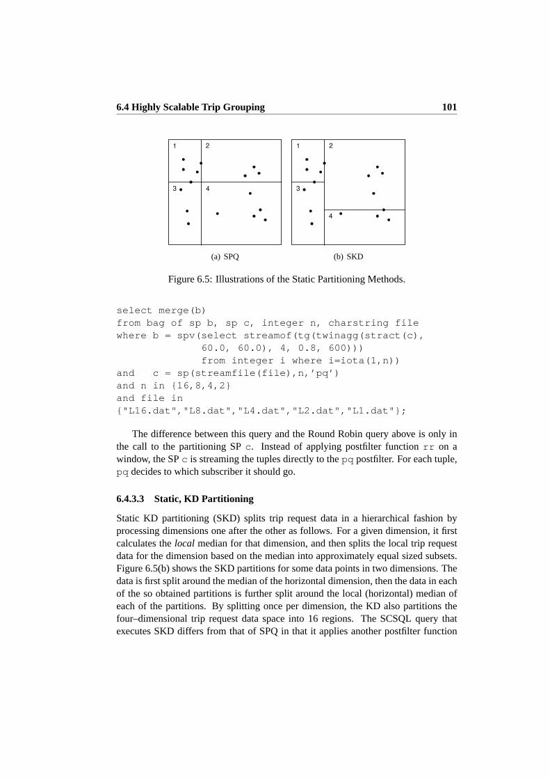
6.4 Highly Scalable Trip Grouping 101
1 2
3 4
(a) SPQ
1 2
3
4
(b) SKD
Figure 6.5: Illustrations of the Static Partitioning Methods.
select merge(b)from bag of sp b, sp c, integer n, charstring filewhere b = spv(select streamof(tg(twinagg(stract(c),
60.0, 60.0), 4, 0.8, 600)))from integer i where i=iota(1,n))
and c = sp(streamfile(file),n,’pq’)and n in 16,8,4,2and file in"L16.dat","L8.dat","L4.dat","L2.dat","L1.dat";
The difference between this query and the Round Robin query above is only inthe call to the partitioning SPc . Instead of applying postfilter functionrr on awindow, the SPc is streaming the tuples directly to thepq postfilter. For each tuple,pq decides to which subscriber it should go.
6.4.3.3 Static, KD Partitioning
Static KD partitioning (SKD) splits trip request data in a hierarchical fashion byprocessing dimensions one after the other as follows. For a given dimension, it firstcalculates thelocal median for that dimension, and then splits the local trip requestdata for the dimension based on the median into approximately equal sized subsets.Figure 6.5(b) shows the SKD partitions for some data points in two dimensions. Thedata is first split around the median of the horizontal dimension, then the data ineachof the so obtained partitions is further split around the local (horizontal) median ofeach of the partitions. By splitting once per dimension, the KD also partitions thefour–dimensional trip request data space into 16 regions. The SCSQL query thatexecutes SKD differs from that of SPQ in that it applies another postfilter function
102 Highly Scalable Trip Grouping for Large–Scale CT Systems
at the partitioning SP, namelykd instead ofpq . Since the difference is so small, theSCSQL query is omitted.
6.4.3.4 Adaptive, Point Quad Partitioning
In many applications, the distribution of the data changes over time, as it is the casefor trip requests. These changes can be minor or major changes. For example, duringthe morning rush hours people want to move from their homes (residential district)to their work (business and industrial districts). During the evening rush hours theopposite is true. The trip requests that correspond to the morning rush hour move-ments are likely to fall in different partitions than the trip requests that correspond tothe evening rush hour movements. Consequently, the “morning rush hour”partitionswill be densely populated in the morning hours, and the “evening rush hour” parti-tions will be densely populated in the evening hours. Clearly, a static partitioningmethod does not consider these changes in data distribution and is likely to result intemporally unbalanced partitions.
The adaptive point quad partitioning (APQ) adjusts the boundaries of the parti-tions periodically, based on statistics obtained from a recent history buffer of the triprequest stream, and distributes the newly arriving trip requests according the newlyadjusted partitions. Figure 6.6(a) shows two consecutive partitionings thatare con-structed by the APQ partitioning for some data points in two dimensions. Hollowdots represent data points that were present when the previous partitioning was con-structed, but are not present or are not relevant for the construction of the currentpartitioning. In contrast, solid rectangular markers represent data pointsthat werenot present when the previous partitioning was constructed, but are relevant for theconstruction of the current partitioning. Solid and dashed lines represent current andprevious partition boundaries. The following SCSQL query executes APQ:
select merge(b)from bag of sp b, sp c, integer n, charstring filewhere b = spv(select streamof(tg(twinagg(stract(c),
60.0, 60.0), 4, 0.8, 600)))from integer i where i=iota(1,n))
and c = sp(pqstat(streamfile(file),600.0, 60.0, 10),n,’pq’)
and n in 16,8,4,2and file in"L16.dat","L8.dat","L4.dat","L2.dat","L1.dat";
This query differs from the SPQ query in the call to the partitioning SPc . Thestreamfile function is wrapped by pqstat(inputstream, size,

6.4 Highly Scalable Trip Grouping 103
1 2
3 4
(a) APQ
1 2
3
4
(b) AKD
Figure 6.6: Illustrations of the Dynamic Partitioning Methods.
stride, samplefreq) . This function emits the same stream as its input stream,and maintains statistics in a main memory table of SCSQ. Everystride ×samplefreq seconds,pqstat computes medians in each dimension oflo × ldacross the tuples seen in the lastsize seconds. These median values are then usedin the pq postfilter. This way, the partitioning decisions are always done on recentdata.
6.4.3.5 Adaptive, KD Partitioning
The adaptive KD partitioning (AKD) adjusts the boundaries of the partitions peri-odically, based on statistics obtained from a recent history buffer of the trip requeststream. and distributes the newly arriving trip requests according the newlyadjustedpartitions. Figure 6.6(b) shows two consecutive partitionings that are constructed bythe AKD partitioning for some data points in two dimensions. The semantics of thesymbols used in the figure are the same as in the case of the APQ partitioning. How-ever, Figure 6.6(b) depicts a situation that can happen in either one of the adaptivespatial partitioning methods. Consider the data point inside the triangle. Since itwaspresent when the previous partition was constructed it has been assigned to computenode 2 for processing. According to the newly constructed partitions however, itshould be assigned to compute node 4. To avoid communication between computenodes, the following design choice is made: once a data point is assigned to apar-tition (compute node), it is never reassigned to another partition, even if the newlyadjusted partitions would suggest this.
The SCSQL query that executes SKD differs from SPQ in that it applies an-other statistics wrapper function and another postfilter function at the partitioning SP,namelykdstat instead ofpqstat andkd instead ofpq . kdstat works analo-gously topqstat with the difference that it maintains dynamical versions of local

104 Highly Scalable Trip Grouping for Large–Scale CT Systems
dimension splits of the kind that SKD has. Since the difference between this queryand the APQ query is so small, the SCSQL AKD query is omitted here.
6.5 Density–Based Spatial Stream Partitioning
The main objective of the four proposed partitioning methods is to load balancetheparallel versions of the computationally intensive TG algorithm. The planes for sub-dividing the space of requests is determined by the medians of request data. Thesesplitting planes potentially eliminate the discovery of good shares, when membersofthe good shares are distributed to different partitions. This naturally leadsto somedegradation in the overall grouping. The degradation is larger when the planes arecutting through denser regions of the request space with many sharing opportunities,than when the planes are cutting through sparser regions of the requestspace. Sinceneither of the proposed partitioning methods consider other characteristicsof the dis-tribution of the requests, the degradation of grouping quality due to boundary effectsis expected to be approximately the same for all four partitioning methods. However,as Section 6.6 demonstrates, this degradation is rather small.
No matter how small the degradation is, simple spatial partitioning methods thattake into account the density of the data could reduce the degradation. Theobjec-tive of such a density–based partitioning is to determine the positions of the splittingplanes so that they pass through regions where data is sparse. To achieve this, a simplebut effective clustering method [29] can be used to find local minima in the multi-modal data distributions along each dimension, and place splitting planes at thoselocations. Figure 6.7 shows the distributions for each dimension of the request dataduring morning peak hours and off–peak hours. In the figure letters “f” and “t” standfor “from” and “to”, respectively. Hence, fx and fy are request origin dimensions,while tx and ty are request destination dimensions. During the morning peak hours,there does not seem to be any regions where the request data is very sparse. However,during off–peak hours, when people who are not working are most likely to be in oneof the larger shopping malls, the distributions of the destination dimensions (tx, ty)are clearly multimodal. In this later situation, ensuring that splitting planes are cho-sen correctly at local minima would minimize the boundary effects. However, sincemost of the requests are during peak hours, the overall average grouping achieved bythe parallel TG algorithm would not be substantially improved.
Since the local minima are likely not to be at the median values of the dimensions,there exists a trade–off between equal–sized partitions and partitions with minimalboundary effects. A dual–objective partitioning that takes this trade–offinto con-sideration could weigh the expected degradation against the imbalance between thecreated partitions. Although the implementation of the density–based and the dual–

6.6 Experiments 105
7.18 7.2 7.22 7.24 7.26 7.28
x 105
0
0.5
1
1.5
2x 10
4
fx6.17 6.175 6.18
x 106
0
0.5
1
1.5
2x 10
4
fy7.2 7.25 7.3
x 105
0
1
2
3
4
5
x 104
tx6.17 6.175 6.18 6.185
x 106
0
0.5
1
1.5
2
2.5
3
3.5
4
x 104
ty
(a) Morning Peak Hours.
7.18 7.2 7.22 7.24 7.26 7.28
x 105
0
2000
4000
6000
8000
10000
12000
fx6.17 6.175 6.18
x 106
0
2000
4000
6000
8000
10000
fy7.2 7.22 7.24 7.26
x 105
0
5000
10000
15000
20000
tx6.17 6.172 6.174 6.176 6.178
x 106
0
5000
10000
15000
ty
(b) Off–Peak Hours.
Figure 6.7: Request Data Distributions Along Each Dimension.
objective spatial stream partitioning methods is straight–forward, it is left for futureresearch.
The proposed spatial stream partitioning methods are devised to scale the TGal-gorithm to very large flows of requests. However, they can be considered as a generalapproach to make computationally intensive spatial analysis tasks scalable throughparallelization. For example, the density–based and the dual–objective spatial streampartitioning methods can be applied to speed up spatial clustering of streams, spatio–temporal rule mining [30], or the processing of high–resolution image streams.
6.6 Experiments
The parallel implementations of the TG algorithm were tested on a cluster of IntelR©
PentiumR© 4 CPU 2.80GHz PCs. Each SP was executing on a separate PC to allow formaximum parallelism. TCP/IP over Fast Ethernet was used to carry streams betweenthe nodes.
Trip request data was simulated using ST–ACTS, a spatio–temporal activity sim-ulator [31]. Based on a number of real world data sources, ST–ACTS simulatesrealistic trips of approximately 600,000 individuals in the city of Copenhagen,Den-
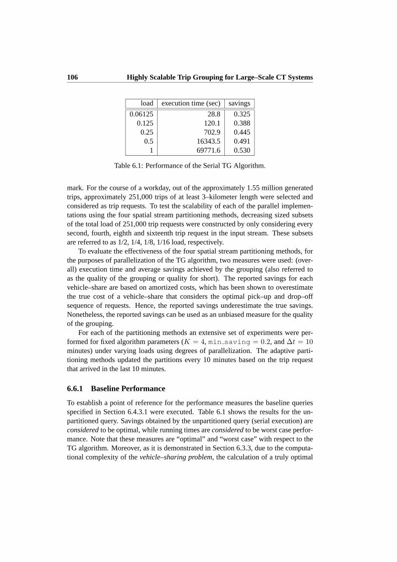
106 Highly Scalable Trip Grouping for Large–Scale CT Systems
load execution time (sec) savings
0.06125 28.8 0.3250.125 120.1 0.3880.25 702.9 0.4450.5 16343.5 0.491
1 69771.6 0.530
Table 6.1: Performance of the Serial TG Algorithm.
mark. For the course of a workday, out of the approximately 1.55 million generatedtrips, approximately 251,000 trips of at least 3–kilometer length were selectedandconsidered as trip requests. To test the scalability of each of the parallel implemen-tations using the four spatial stream partitioning methods, decreasing sized subsetsof the total load of 251,000 trip requests were constructed by only considering everysecond, fourth, eighth and sixteenth trip request in the input stream. These subsetsare referred to as 1/2, 1/4, 1/8, 1/16 load, respectively.
To evaluate the effectiveness of the four spatial stream partitioning methods, forthe purposes of parallelization of the TG algorithm, two measures were used:(over-all) execution time and average savings achieved by the grouping (also referred toas the quality of the grouping or quality for short). The reported savings for eachvehicle–share are based on amortized costs, which has been shown to overestimatethe true cost of a vehicle–share that considers the optimal pick–up and drop–offsequence of requests. Hence, the reported savings underestimate the true savings.Nonetheless, the reported savings can be used as an unbiased measurefor the qualityof the grouping.
For each of the partitioning methods an extensive set of experiments were per-formed for fixed algorithm parameters (K = 4, min saving = 0.2, and∆t = 10minutes) under varying loads using degrees of parallelization. The adaptive parti-tioning methods updated the partitions every 10 minutes based on the trip requestthat arrived in the last 10 minutes.
6.6.1 Baseline Performance
To establish a point of reference for the performance measures the baseline queriesspecified in Section 6.4.3.1 were executed. Table 6.1 shows the results for the un-partitioned query. Savings obtained by the unpartitioned query (serial execution) areconsideredto be optimal, while running times areconsideredto be worst case perfor-mance. Note that these measures are “optimal” and “worst case” with respect to theTG algorithm. Moreover, as it is demonstrated in Section 6.3.3, due to the computa-tional complexity of thevehicle–sharing problem, the calculation of a truly optimal

6.6 Experiments 107
grouping, even in the case of a few requests, is infeasible. Due to the large differ-ence in scale between serial and parallel execution times, serial executiontimes arenot shown in subsequent figures. Savings achieved by the unpartitioned query (serialexecution) are also not shown in subsequent figures, but are used toreport relativeperformance of the parallel executions in terms of savings / quality.
In comparison, the round robin query was executed to obtain optimal executiontimes due to perfect load balancing and worst case savings due to the query indepen-dent distribution of data between query processors. The results of these experimentsare shown in Figures 6.8 and 6.9 as RR, however it is emphasized that RR isnot oneof the proposed spatial stream partitioning methods, but isonlyused as a reference.
6.6.2 Absolute Performance of the Parallel TG Algorithms
Figures 6.8 and 6.9 show the absolute performance of the parallel TG algorithm forvarying load and degrees of parallelization using different spatial stream partitioningmethods. From Figure 6.8(a) it can be seen that the execution times of all of themethods decrease as the parallelism is increased. Figure 6.8(a) also reveals that theadaptive versions of the spatial partitioning methods adjust well to the changing spa-tial distribution of the requests, resulting in more balanced partitions and ultimatelyfaster execution times when compared to their static version. The improvement inexecution time due to adaptive partitioning is most evident for the SPQ partitioning.Figure 6.8(b) shows that while the execution time of the TG algorithms can be scaled,the underlying algorithmic complexity of the TG algorithm executed on the computenodes does not change. The effect of the underlying algorithmic complexity is moreobservable for spatial partitioning methods that construct less balanced partitionings,in particular SPQ.
Figure 6.9(a) shows that in general the quality of the grouping decreases as thedegree of parallelization is increased. However in the case of non–spatial partitioning(RR) this degradation is significant, while in the case of either one of the fourspatialpartitioning methods it is negligible. Figure 6.9(b) shows that as the load is increasedthe grouping quality increases. This is due to the simple fact that the spatio–temporaldensity of the trip requests increases. As a consequence, the likelihood that a requestbecomes part of a “good” vehicle share increases. The almost negligibledifferencesbetween the qualities achieved by the four partitioning methods, as explained inSec-tion 6.5, is due to the fact that since neither of the partitioning methods considerthedata densities, but only the medians of the dimensions, the total degradation due toboundary effects is approximately the same for the four partitioning methods.

108 Highly Scalable Trip Grouping for Large–Scale CT Systems
2 4 8 160
5000
10000
15000
20000
25000
30000
# of processors
exec
utio
n tim
e (s
ec)
Execution time full load
RRSPQSKDAPQAKD
(a) Performance for Full Load.
0.0625 0.125 0.25 0.5 10
500
1000
1500
2000
load
exec
utio
n tim
e (s
ec)
Execution time 16 processors
RRSPQSKDAPQAKD
(b) Performance for 16 Processors.
Figure 6.8: Execution Times for the Parallel TG Algorithm for Different PartitioningMethods for Varying Parallelization and Load.

6.6 Experiments 109
2 4 8 160
0.1
0.2
0.3
0.4
0.5
0.6
0.7
# of processors
savi
ngs
Savings full load
RRSPQSKDAPQAKD
(a) Quality for Full Load.
0.0625 0.125 0.25 0.5 10
0.1
0.2
0.3
0.4
0.5
0.6
0.7
load
savi
ngs
Savings 16 processors
RRSPQSKDAPQAKD
(b) Quality for 16 Processors.
Figure 6.9: Savings for the Parallel TG Algorithm for Different PartitioningMethodsfor Varying Parallelization and Load.

110 Highly Scalable Trip Grouping for Large–Scale CT Systems
2 4 8 160
10
20
30
40
50
# of processors
exec
tim
e / o
ptim
al p
aral
lel
exec
tim
e Relative execution time full load
SPQSKDAPQAKD
Figure 6.10: Relative Performance for the Parallel TG Algorithm (Compared to RRPartitioning) for Different Partitioning Methods for Varying Parallelization.
6.6.3 Relative Performance of the Parallel TG Algorithms
Figure 6.10 shows relative execution times of the parallel TG algorithms when com-pared to the optimal execution time that is achieved by RR partitioning due to perfectload balancing. With the exception of the SPQ partitioning all other partitioningmethods result in parallel execution times that are within the same order of magni-tude as the optimal. There are potentially two sources for this slowdown: the cost ofpartitioning and the extended execution times due to improper load balancing. Sinceadaptive partitioning methods have to maintain a limited history of the stream andperiodically recompute partition boundaries based on this history, they do additionalwork compared to their static counterparts. Yet, in Figure 6.10 execution times re-sulting from adaptive partitioning are significantly lower than the execution timesachieved by static partitioning. Hence, it is clear that the additional time neededtoperform the spatially partitioned parallel queries can mainly be attributed to unbal-anced partitions.
Finally, comparing the savings in Figure 6.9(b) to the savings in Table 6.1 revealsthat the grouping quality achieved by either one of the partitioning methods is withinthe 95% of the optimal quality for the full load. Even if the load is decreased to 1/16of the total load, all the spatial partitioning methods still achieve approximately 90%of the maximum possible savings.

6.7 Conclusions and Future Work 111
The experiments can be summarized as follows. First, RR partitioning has per-fect load balance and is a very simple partitioning method, hence it has the fastestexecution time. However, RR partitions the space badly and achieves a bad groupingquality. Second, using a spatial partitioning method improves grouping quality.Allspatial partitioning methods achieve at least 95% of the maximum possible savings incase of the full load. Third, the adaptive partitioning methods always execute fasterthan their static equivalents. That is because the adaptive methods constantly adaptthe partitioning according to the last tuples observed, which will lead to better loadbalance. At the same time, the savings are approximately the same for both the staticand dynamic partitionings. Adaptive partitioning is also preferred from an operationpoint of view, since it does not need any prior knowledge about the datadistribution.Finally, since all partitioning methods (except RR) achieve about the same savings,the preferred method is the one with the fastest execution time of SPQ, SKD, APQ,and AKD. Thus, AKD is the best partitioning method.
6.7 Conclusions and Future Work
The paper proposed highly scalable algorithms for trip grouping to facilitate large–scale collective transportation systems. The algorithms are implemented using a par-allel data stream management system, SCSQ. First, the basic trip grouping algorithmis expressed as a continuous stream query in a data stream management system toallow for a very large flow of requests. Second, following the divide–and–conquerparadigm, four spatial stream partitioning methods are developed and implementedto divide the input request stream into sub–streams. Third, using the infrastructureof SCSQ and the partitioning methods, parallel implementations of the grouping al-gorithm are executed in a parallel computing environment. Extensive experimen-tal results show that the parallel implementation using simple, adaptive partitioningmethods can achieve speed–ups of several orders of magnitude withoutsignificantlyaffecting the quality of the grouping. As discussed in Section 6.5, spatial partitioningis not only appropriate for the given application, but it is applicable to parallelizecomputationally expensive spatial analysis tasks. As it was demonstrated, SCSQ caneasily accommodate the parallel implementations of such tasks.
Future work will be along four paths. First, for the adaptive partitioning methods,the effects of keeping a longer history versus sampling more frequently willbe in-vestigated. Second, the density–based and dual–objective spatial stream partitioningmethods will be implemented and their effectiveness evaluated. Third, the proposedpartitioning methods, independent of the rate of flow, always construct afixed num-ber of partitions. While not substantially, but as the number of partitions increasesthe grouping quality decreases. Hence, an adaptive partitioning approach in whichthe number of partitions is increased / decreased depending on the rate offlow will

112 Highly Scalable Trip Grouping for Large–Scale CT Systems
be devised and tested. Finally, to preserve clarity the paper presented thegeneric TGalgorithm in its simplest form. In particular, in the presented version all vehicles areassumed to have the same passenger capacity and all requests have a common min-imum savings parameter. Furthermore, in–route grouping, i.e., assigning requeststo already active but not fully–occupied vehicle–shares, is not handled by the simpleversion of the TG algorithm. Future work will consider the implementation of a morecomplex version of the TG algorithm that addresses the above issues.

Chapter 7
Estimating the Capacity of theLocation–Based AdvertisingChannel
Delivering “relevant” advertisements to consumers carrying mobile devices is re-garded by many as one of the most promising mobile business opportunities. Therelevance of a mobile ad depends on at least two factors: (1) theproximity of themobile consumer to the product or service being advertised, and (2) the match be-tween the product or service and theinterestof the mobile consumer. The interestof the mobile consumer can be eitherexplicit (expressed by the mobile consumer)or implicit (inferred from user characteristics). This paper tries to empirically esti-mate the capacity of the mobile advertising channel, i.e., the number of relevant adsthat can be delivered to mobile consumers. The estimations are based on a simu-lated mobile consumer population and simulated mobile ads. Both of the simulateddata sets are realistic and derived based on real world data sources about populationgeo–demographics, businesses offering products or services, andrelated consumersurveys. The estimations take into consideration both the proximity and interestre-quirements of mobile ads, i.e., ads are only delivered to mobile consumers that areclose–by and are interested, where interest is either explicit or implicit. Results showthat the capacity of the Location–Based Advertising channel is rather large, which isevidence for a strong business case, but it also indicates the need for user–control ofthe received mobile ads.
113
114 Estimating the Capacity of the Location–Based Advertising Channel
7.1 Introduction
Mobile or Location–Based Advertising (MA or LBA), i.e., sending electronicadver-tisements to consumers carrying mobile devices, is considered by many as oneof themost promising business opportunities amongst Location–Based Services (LBS) [62].A recent mobile marketing survey suggests that about 7% of the mobile consumerswould be willing to receive promotional text messages “if they were relevant”[27].According to other surveys, an even larger percentage of the mobile consumers are in-terested if they are rewarded in some way [66]. In this paper, mobile ads are regardedas a means of presenting relevant information to a recipient, be it a commercialofferon an item on sale, traffic information, or a piece of public information. To manypeople, the world seems to be more and more difficult to guide oneself through, thusthe art of targeting information and services will prove to be of immense value.Only,efficient business cases have so far been very few, in spite of the market’s expecta-tions.
A broad range of aspects, or variables, determine the relevance and context of amobile ad: distance to the mobile user, explicit or implicit interest of the mobile user,uniqueness (do not send ad twice within some interval), time and place of delivery,etc. To this extent, this paper describes an LBA framework and an LBA database thatcan be used for the management of mobile advertisements.
In lack of comprehensive, real data on the movements and behavior of thepopu-lation, estimation or simulation is extremely useful, bringing the models to life withreal and well–documented consumption patterns. Using a simulated but realisticmo-bile consumer population and a set of mobile ads, the LBA database is used to esti-mate the capacity of the mobile advertising channel, i.e., the number of relevant adsthat can be delivered to mobile consumers. Apart from this use, the LBA databaseand the estimates derived from it can also be used in mobile catchment area analysisto estimate business exposure. Results show that the capacity of the LBA channelis rather large (approx. 100 mobile ads per user within a single day), giving strongsupport for a business case. The same results can also be viewed as alarming, andindicate the need to incorporate user–control of the received mobile ads inthe LBAframework, as suggested by the Mobile Marketing Association [73].
The remainder of this paper is organized as follows. Section 7.2 reviews relatedwork. Section 7.3 defines the estimation problem both in case of explicit and implicitinterest. Section 7.4 describes the simulated data sets and their derivations fromreal–world data sources. Section 7.5 describes the method and technical foundationsfor delivering mobile ads while taking into account both the advertisers’ andmobileusers’ interests. Section 7.6 proposes a revenue model for LBA. Section 7.7 describesthe experiments and discusses the estimates resulting from them. Finally, Section7.8concludes and points to future research directions.

7.2 Related Work 115
7.2 Related Work
The estimations in this work are based on simulated movements of mobile users.Movements of users are influenced by physical, social and geo–demographical as-pects of mobility. To aid the development in mobile data management, a number ofmoving object simulators have been proposed in the literature that model primarilythe physical aspects of mobility to various extents. Since most objects use a networkto get from one location to the other, a state–of–the–art framework for network–basedmoving object simulation is presented in [8]. The behavior of a moving object inthisframework is influenced by (1) the attributes of the object having a particular objectclass, (2) the combined effects of the locations of other objects and the network ca-pacity, and (3) the location of external objects that are independent of the network.For a review of other moving object simulators the reader is referred to [31].
Moving object simulators generally neglect the social and geo–demographical as-pects of mobility. These social and geo–demographical aspects of mobility introducepatterns in the movement of users and give rise to a unique spatio–temporal (ST)distribution of users. ST–ACTS is a Spatio–Temporal ACTivity Simulator that usingreal–world data sources models some of these neglected aspects of mobility [31]. Tomake the estimations in this work as realistic as possible, movements of mobile usersare obtained from ST–ACTS, which is further described in Section 7.4.4.
Database indices allow the effective management and retrieval of data in largedatabases. Spatial and geographical databases manage information about spatial ob-jects, i.e., objects that have physical properties such as location and extent. An R–treeis a widely used index structure that allows the effective management and retrievalof spatial objects [45]. An R–tree splits space with hierarchically nested, and pos-sibly overlapping Minimum Bounding Rectangles (MBRs). Search algorithms thattest spatial relationships (for example; intersection, containment, nearest)betweenspatial objects can effectively use the MBRs to decide whether or not objects in twoMBRs satisfy a specific spatial search criterion.
The location of a moving object changes over time. Thus, the path of a mov-ing object is commonly described as a sequence of coordinate and timestamp pairsand is referred to as the trajectory of the moving object. Moving objects databasesare databases that represent and manage changes related to the movement of ob-jects. Spatio–temporal indices such as the Spatio–Temporal R–tree (STR–tree) andTrajectory–Bundle tree (TB–tree) allow the effective management and retrieval ofinformation about moving objects [55]. An STR–tree organizes line segmentsof atrajectory according to both their spatial properties and the trajectories theybelong to,while a TB–tree only preserves trajectories. While these spatio–temporal indices aredesigned to effectively manage trajectories, they are not available in commercially

116 Estimating the Capacity of the Location–Based Advertising Channel
available Relational Database Management Systems (RDBMSs). Hence, thehereinpresented method uses the widely available R–trees.
Time geography [46] is a conceptual basis / paradigm for human space–time be-havior which considers (1) the indivisibility or corporeality of the human condition;(2) that humans typically operate over finite intervals of space and time; (3) the natu-ral laws and social conventions that partially constrain space–time behavior; and (4)that humans are purposive. The movements of mobile users used in the estimationsare derived from ST–ACTS [31], which models some aspects of this paradigm.
Research has shown that LBSes have not yet been as widely used as expected [60].In opposition to earlier forecasts and market expectations, technology has not beenready until now. Furthermore, and no less important, is that the user and theuserneeds have not been fully understood. Recent research shows thatin order to suc-ceed with location–based ads, content is imperative [61], as well as takingthe con-sumers’ permission, acceptance and responsiveness into account is crucial [5, 50].Being aware of this, the concept proposed in the present paper takes off from a pointwhere any user will benefit directly from the use of the system, thus leadingto anincreased opt–in readiness.
Ensuring full user responsiveness is by no means trivial; research indicates thatbehavioral intention to use mobile commerce can be greater for mobile commerce–nonusers than for users. Those most used to mobile commerce are not as prone to takeaction on it. However, although this documents that the triggers of mobile commerceacceptance is not yet fully understood [65], mobile users are found to be eager tomake use of their phones in new ways, and methodologies are proposed to modeluser willingness [24, 66, 78]. In the present paper, by targeting content to the rightrecipients, the setup is realistic and should be attractive for the typical future user.
Market research document a significant increase in sales to customers who wereexposed to mobile advertising compared to those who were not exposed [72]. Inother words, it works, if only the above mentioned issues are treated seriously. It isthe intention with the present paper to contribute in furthering the spread of LBSes.
7.3 Problem Statement
Let A = a1, . . . an be the set of ads. Each ada has a locationadloc(a) and is fora certain productprod(a). Let U = u1, . . . un be the set of (moving) users. Eachuseru has a locationuloc(u, t) depending on the timet, an explicit interest profileexpint(u) containing a set of products, and an implicit interest profileimpint(u),containing a set of demographic variable values. Also assume a scoring functionscore(u, a) that given a useru and an ada returns a value between 0 (no match) and1 (perfect match) that predicts how interested useru is in productprod(a) based onthe values inimpint(u).

7.4 Data 117
referred entity conzoomR© variable categories
person
person count 1age 9education type 9employment status type 12employment branch type 12
housing unit
unit count 1house type 6house ownership type 4house area 5
household
household count 1family type 5fortune 6personal income 5
Table 7.1: Variables in conzoomR©.
Given a maximum distancemaxdistbetween user locations and ad locations, anda timespanT = [tstart : tend], the explicit location–based ad delivery estimationproblem is to estimate how many times a useru has a locationuloc(u, t) withinmaxdistfromadloc(a) for an ada in A and a timet in T whereprod(a) ∈ expint(u).
Given amaxdistbetween user locations and ad locations, aminscore, and a times-panT = [tstart : tend], the implicit location–based ad delivery estimation problemis to estimate how many times a useru has a locationuloc(u, t) within maxdistfromadloc(a) for an ada in A and a timet in T wherescore(u, a) ≥ minscore.
7.4 Data
The estimations stated in Section 7.3 are based on a number of real–world datasources. The use of real–world data sources is important to derive realistic esti-mates. While the data sources refer to the Danish market and population, similardatasources are available for other major markets [18, 19]. The following subsectionsdescribe in detail the data sources used to derive the estimates.
7.4.1 conzoomR© Demographic Data
conzoomR© is a commercial database product that contains fine–grained, geo–demo-graphic information about Denmark’s population [28]. The variables thatdescribe thestatistical characteristics of the population can be divided into three groups: person,housing unit, and household variables. These variables and the number of categoriesfor each are shown in Table 7.1.

118 Estimating the Capacity of the Location–Based Advertising Channel
In Table 7.1, variables that have “type” in their names are categorical variables;variables that have “count” in their name are counts of the correspondingentitieswithin a 100–meter grid cell; and finally, the rest of the variables are continuousvariables that have been categorized into categories that are meaningfulfor marketsegmentation. Since, for example in the countryside, the number of persons, house-holds or units could be very low in a 100–meter grid cell, grid cells are groupedtogether into meaningful, large enough clusters to comply with social and ethicalnorms and preserve the privacy of individuals. The basis for clustering is twofold:geography and the publicly available one–to–one housing information. Theintuitionbehind the basis is also twofold. First, people living in a given geographical region(be that a state, a county, or a postal district) are similar in some sense; for example,they might be more likely to have a certain political orientation than people livingin another geographical region. Second, people living in similar houses are likely tobe similar in other demographic variables; for example an established family witha stable source of income is more likely to be able to buy a larger, more expensivehouse than a person who just started his/her career.
As mentioned earlier, to preserve the privacy of individuals, the clustersare con-strained to contain at least some fixed number of households. Statistics for the vari-ables, depending on the sensitivity of the information contained in them, are obtainedfrom Statistics Denmark [85] for clusters constructed at an appropriate level of clus-ter size constraint, for example 20, 50, 100, and 150 households per cluster. In case ofa continuous variable, for example age, counts of the corresponding entities (in thiscase persons in the cluster) are obtained for the categories of the givenvariable. Dueto this constrained geo–clustering method, the conzoomR© clusters obtained complywith the social and ethical norms and preserve the privacy of the individual, yet thestatistics obtained are accurate enough for effective market segmentation. This seg-mentation results in a grouping of the Danish population into 29 conzoomR© types,one of which is defined for each 100–meter grid cell. Cosmopolitan (type 3) isoneexample of the 29 conzoomR© types. Comparing the demographics of type 3 to thedemographics of the rest of Denmark’s population gives the demographicprofile ofthe type. This profile is partially shown in Figure 7.1. It roughly describes individu-als that are more likely: to be middle aged (30–59 years old), to live in larger citiesin larger, multi–family houses that are either owned by them or are private rentals, tobe mostly couples with children, to have a medium to long higher education, to holdhigher level or top management positions in the financial or public sector, and to havea better household economy (in terms of wealth and income) than the average Dane.
7.4.2 GallupPCR© Consumer Survey Data
GallupPCR© is a commercial database product and as the name suggests, it containsdetailed survey responses of consumers about their demographics; interests such as

7.4 Data 119
−100 −50 0 50 100 150 200
pp_age_0_11pp_age_12_16pp_age_17_22pp_age_23_29pp_age_30_39pp_age_40_49pp_age_50_59pp_age_60_65pp_age_66plushp_edu_basicSchoolhp_edu_generalUpperSchoolhp_edu_vocationalUpperSchoolhp_edu_vocationalTraininghp_edu_shortHighhp_edu_mediumHighhp_edu_bachelorhp_edu_longHighResearchhp_edu_unknownpp_empl_selfpp_empl_topManagementpp_empl_upperLevelpp_empl_mediumLevelpp_empl_basicLevelpp_empl_cashBenefitpp_empl_earlyRetirementpp_empl_jobReleasePensionpp_empl_studentpp_empl_oappp_empl_restpp_empl_restChildrenpp_empl_agriculturepp_empl_manufacturingpp_empl_supplypp_empl_constructionpp_empl_tradepp_empl_transportpp_empl_financialpp_empl_publicpp_empl_unknownpp_empl_notOccupiedChildrenpp_empl_notOccupiedAdultpp_empl_notOccupiedOldAge
Type 3 − Cosmopolitan vs Denmark
Index weighted by households−100 −50 0 50 100 150 200
Type3 15.9 % DK 15.1 %Type3 05.6 % DK 06.1 %Type3 05.7 % DK 06.4 %Type3 07.5 % DK 08.6 %Type3 16.5 % DK 14.7 %Type3 15.4 % DK 14.2 %Type3 15.4 % DK 13.8 %Type3 06.7 % DK 06.9 %Type3 11.3 % DK 14.1 %Type3 09.7 % DK 24.2 %Type3 05.0 % DK 04.1 %Type3 01.4 % DK 01.6 %Type3 24.5 % DK 36.5 %Type3 05.6 % DK 05.0 %Type3 19.8 % DK 14.2 %Type3 02.6 % DK 01.6 %Type3 26.0 % DK 07.2 %Type3 05.5 % DK 05.4 %Type3 04.0 % DK 03.7 %Type3 02.3 % DK 01.2 %Type3 14.7 % DK 05.9 %Type3 10.8 % DK 08.0 %Type3 23.2 % DK 31.4 %Type3 00.5 % DK 01.0 %Type3 02.1 % DK 04.1 %Type3 02.2 % DK 03.3 %Type3 02.9 % DK 02.6 %Type3 09.8 % DK 12.0 %Type3 07.5 % DK 07.4 %Type3 20.0 % DK 19.5 %Type3 00.2 % DK 01.7 %Type3 04.4 % DK 07.8 %Type3 00.3 % DK 00.3 %Type3 01.8 % DK 03.1 %Type3 07.8 % DK 09.1 %Type3 03.4 % DK 03.2 %Type3 12.4 % DK 06.9 %Type3 24.3 % DK 18.0 %Type3 00.4 % DK 00.3 %Type3 20.0 % DK 19.5 %Type3 11.0 % DK 11.0 %Type3 14.1 % DK 19.4 %
Figure 7.1: Partial Profile of conzoomR© Type 3.
culture, hobbies, and sports household consumptions, purchasing habits; transporta-tion habits; views on various subjects; attitudes and exposure to various advertise-ment media [26]. The questions in the surveys are yes/no questions. To measure themagnitude of the consumer’s interest in a specific area, the original yes/noquestionis re–phrased as categorical questions. For example the original yes/noquestion “Areyou interested in fashion?” is re–phrased to 5 yes/no questions using the followinganswer possibilities: very, rather, somewhat, not very, or not interested.
7.4.3 bizmarkTM
Products and Services
bizmarkTM
is a commercial database product that contains detailed information aboutDanish businesses both in the public and the private sector [28]. Some of the one–to–one information that is available about businesses is their location, the numberof employees working in them, the physical size of the business facility, and theinternational branch codes the businesses fall under. Using the hierarchy of inter-

120 Estimating the Capacity of the Location–Based Advertising Channel
national branch codes 40 product and service categories were identified for whichrelated consumer surveys were also available. The product and service categories areas follows: classical concert; pop/rock concert; discotheque; art exhibition; museum;cinema; theater; pharmacy; bicycle / moped; car, stereo/HI–FI; CDs/DVDs; com-puter/internet; new technologies/telecommunication; do–it–yourself; fashion; cos-metics/skincare; glasses/contacts; hairdresser; jeweler/watches; interior design; travel;pets, fast–food; and 14 brand specific supermarkets. Based on the internationalbranch codes a one–to–many relationship has been established between asubset ofthe businesses in bizmark
TMand the 40 product / service categories.
7.4.4 Simulating Mobile Users with ST–ACTS
ST–ACTS is a probabilistic, parameterizable, realistic Spatio–Temporal ACTivitySimulator [31]. ST–ACTS is realistic in the sense that it is based on a number ofreal–world data sources (among others, the data sources described above) and a setof principals that try to model thesocial and some of thephysicalaspects of mo-bility. The modelled principles that govern the social aspects of mobility are: (1)People move from a given location to another location with anobjectiveof perform-ing some activity at the latter location; (2) Not all are equally likely to perform agiven activity. The likelihood of performing an activity depends on theinterestof agiven person, which in turn depends on a number of demographic variables; (3) Theactivities performed by a given person are highlycontext dependent. Some importantparts of context are: the current person location, the set of locations where a givenactivity can be performed, the current time, and the recent history of activities of theperson; (4) The locations of facilities where a given activity can be performed, arenot randomly distributed, but areinfluencedby the locationsof other facilities andthe locationsof the users of those facilities.
The output of ST–ACTS is a population of simulated persons, each describedby a set of demographic variables and associated with a trajectory. The trajectoriesare sequences of time–stamped activities performed at particular physicallocations,i.e., coordinates. In addition to the four principles above, the simulated activitiesalso obey the following constraints. First, thetemporal activity constraint, whichstates that certain activities are more likely to be performed during some periods thanothers. Second, theactivity duration constraint, which states that not all activitiestake the same amount of time. Third, themaximum distance constraint, which statesthat for most activities there is a maximum distance a person is willing to travel.Finally, the trajectories assume linear movement between two consecutive activities,i.e. locations, but obey somephysical mobility constraints, namely, that it takestime to move from one location to another. The time it takes to move from onelocation to another is calculated based on the distance between the two locationsand
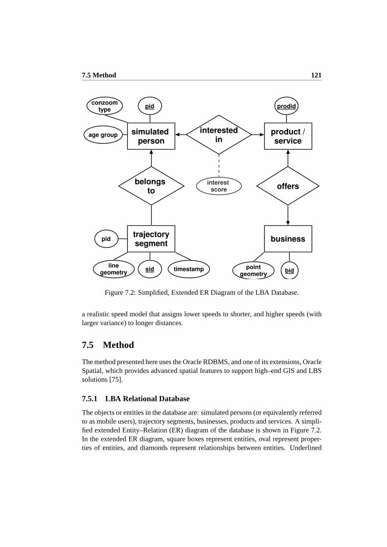
7.5 Method 121
simulated person
trajectorysegment
business
product /service
belongs to
offers
interestedin
linegeometry
pointgeometry
bid
prodidpid
sid
pid
timestamp
conzoomtype
age group
interest score
Figure 7.2: Simplified, Extended ER Diagram of the LBA Database.
a realistic speed model that assigns lower speeds to shorter, and higher speeds (withlarger variance) to longer distances.
7.5 Method
The method presented here uses the Oracle RDBMS, and one of its extensions, OracleSpatial, which provides advanced spatial features to support high–endGIS and LBSsolutions [75].
7.5.1 LBA Relational Database
The objects or entities in the database are: simulated persons (or equivalently referredto as mobile users), trajectory segments, businesses, products and services. A simpli-fied extended Entity–Relation (ER) diagram of the database is shown in Figure 7.2.In the extended ER diagram, square boxes represent entities, oval represent proper-ties of entities, and diamonds represent relationships between entities. Underlined

122 Estimating the Capacity of the Location–Based Advertising Channel
properties represent primary constraints. The arrows between entities encode con-nectivity of relationships, i.e., and arrow represents “one” and no arrow represents“many”. For example, the “belong to” relationship is a many–to–one relationship be-tween trajectory segments and simulated persons, i.e. one trajectory segmentbelongsto exactly one simulated person, but many trajectory segments can belong to one sim-ulated person. Mobile ads are indirectly modelled by in the relational databasethemany–to–many “offers” relationship between businesses and products or services.Through this relationship, a mobile ad can be thought of as an entity having a uniqueidentifier composed of a unique combination ofbid and prodid , and having alocationspecified by thepoint geometryof the business offering the advertisement.
As it was introduced earlier, in the implicit case, the interest of a mobile useru and a mobile ada about a product or serviceprod(a) is not a Boolean functionor binary relation. Rather, it is a continuous function that given the demographiccharacteristicimpint(u) of u, assigns a real valued interest scorescore(u, a), usuallyfrom 0 (not interested) to 1 (very interested), forprod(a). In direct marketing thisfunction is termed a scoring function, which encodes a particular scoring model.This real valued scoring function is untraditionally represented as a property of the“interested in” relationship in the ER diagram.
7.5.2 Proximity Requirements on Mobile Ads
A mobile ada is likely to be considered relevant to a mobile useru only if at thetime of deliveryt, u is (or at some foreseeable future time point will be) within amaximum distance,maxdist, to the origin of the mobile adadloc(a), i.e. the locationof the business. Using the spatial features of Oracle Spatial, this proximity criterionbetween mobile ads and mobile users is tested as follows. The geometries of the busi-nesses, equivalently mobile ads, are buffered to a maximum distance, and tested forany spatial interaction with the geometries of the trajectory segments, by performinga spatial join operation in the database. To make the join operation as fast as possible,geometries are indexed using R–trees.
7.5.3 Interests Based on Demography
The relevance of a mobile ad for a particular product or service is naturally influencedby the interest of the user for the given product or service. As described above, a sub-set of the GallupPCR© consumer survey questions are related to products or servicesthat can be directly linked to businesses in bizmark
TM, and measure the interests of
the consumer in the products or services.Using the geo–demographic parts of the surveys, each survey subjectis assigned
to one of the 29 conzoomR© types. To derive a single indicator, an interest score, forhow interested a given conzoomR© type is in a given product or service, the answers
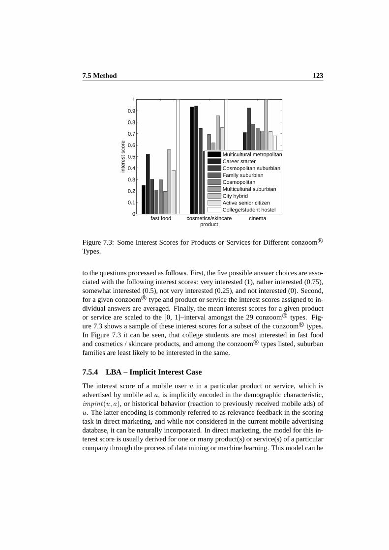
7.5 Method 123
fast food cosmetics/skincare cinema0
0.1
0.2
0.3
0.4
0.5
0.6
0.7
0.8
0.9
1
product
inte
rest
sco
re
Multicultural metropolitanCareer starterCosmopolitan suburbianFamily suburbianCosmopolitanMulticultural suburbianCity hybridActive senior citizenCollege/student hostel
Figure 7.3: Some Interest Scores for Products or Services for Different conzoomR©
Types.
to the questions processed as follows. First, the five possible answer choices are asso-ciated with the following interest scores: very interested (1), rather interested (0.75),somewhat interested (0.5), not very interested (0.25), and not interested (0). Second,for a given conzoomR© type and product or service the interest scores assigned to in-dividual answers are averaged. Finally, the mean interest scores fora given productor service are scaled to the [0, 1]–interval amongst the 29 conzoomR© types. Fig-ure 7.3 shows a sample of these interest scores for a subset of the conzoomR© types.In Figure 7.3 it can be seen, that college students are most interested in fast foodand cosmetics / skincare products, and among the conzoomR© types listed, suburbanfamilies are least likely to be interested in the same.
7.5.4 LBA – Implicit Interest Case
The interest score of a mobile useru in a particular product or service, which isadvertised by mobile ada, is implicitly encoded in the demographic characteristic,impint(u, a), or historical behavior (reaction to previously received mobile ads) ofu. The latter encoding is commonly referred to as relevance feedback in the scoringtask in direct marketing, and while not considered in the current mobile advertisingdatabase, it can be naturally incorporated. In direct marketing, the modelfor this in-terest score is usually derived for one or many product(s) or service(s) of a particularcompany through the process of data mining or machine learning. This model can be

124 Estimating the Capacity of the Location–Based Advertising Channel
represented as acompany–specific interest score functionin the mobile advertisingdatabase that for given user–demographics and historical user–behavior, see Section7.5.8, assigns an interest score to the user. In the estimations however, these interestscore functions are not company– but rather only product– and service–specific. Fur-thermore, due to their simplicity, they are implemented as table with the followingschema:interest score = 〈conzoom type, prodid, score 〉.
7.5.5 LBA – Explicit Interest Case
Mobile users can also explicitly state their interest in certain products and services.In this case the “interested in” relationship is a binary relationship in the mobileadvertising database. To provide a realistic estimates, the explicit interests ofusersare probabilistically simulated by randomly drawing a fixed number of productsforevery mobile user according to the distribution of interest scores given theconzoomR©
type of the user.
7.5.6 Uniqueness and User–Defined Quantitative Constraints on MobileAds
Receiving the same ad multiple times naturally decreases the relevance of the adasthe therein presented information is not new. Primary key constrains in RDBMSsare an effective mechanism for guaranteeing that only unique combinationof mobileusers and mobile ads are considered for delivery. In the mobile marketing data-base the delivered ads are stored in amobile ad delivery table with the fol-lowing schema:〈pid, bid, prodid, delivery time 〉. Placing a primarykey constrain on the first three columns guarantees that a mobile ad is delivered atmost once to a mobile user. Recording thedelivery timeallows the control of there–delivery of mobile ads after a certain period of time has passed. For clarity, themobile ad delivery table is omitted from the ER diagram in Figure 7.2.
As the number of mobile ads increases, or the other constraints on the deliveryof mobile ads weaken, the number of mobile ads delivered to a mobile user willnaturally increase. After a certain number of ads have been delivered tothe user, anyadditionally delivered ad, while maybe relevant, will likely be perceived as annoying.Hence, the mobile user’s ability to limit the number of delivered ads is important.This user–control can be effectively facilitated by the top–k query mechanism whichis provided in most RDBMSs.
7.5.7 User–Defined ST Constraints on Mobile Ads
Time and location are important aspects of the context of mobile ads. Most userswould consider receiving a mobile ad as intrusive or disturbing when receiving it

7.5 Method 125
during work hours or after a certain time in the evening in their homes. Hence,the mobile user’s ability to prevent the delivery of mobile ads in certain regionsofspace and time are important. While the user–control of spatio–temporal constraintson mobile ads is not present in the mobile advertising database, the database canbe easily extended to accommodate for this feature as follows. Users can specifymobile ad profilesby restricting certain spatial and / or temporal regions for mobilead delivery. Then, spatio–temporal joins between the mobile ad profiles andmobileads can be performed to further control the delivery of mobile ads.
7.5.8 Inferring Personal Interests and Relevance Based on HistoricalUser–Behavior
Geo–demographic variables can be used to predict the general interestsof an indi-vidual user, as explained in Section 7.5.3. However, since an individualuser cannotbe perfectly characterized by a few geo–demographic variables, it is likely that thepredicted general interests differ slightly from the true,personal interestsof the indi-vidual user. In the following, two methods are proposed to infer the personal interestsof individual users.
The first method uses the locations that an individual user visits to infer the user’spersonal interests. A subset of the locations a user visits are commercial innature,i.e., are businesses that offer products or services. During the lifetime ofa user, thefrequencies of how often the user visits particular businesses or types of businessesthat offer particular products or services, can be recorded. Furthermore, periodicalpatterns can also be easily detected in the sequence of visits. An example of sucha simple periodical pattern would be that a user visits a hairdresser approximatelyevery second month. Basing the delivery of mobile ads on the personal frequen-cies of visited locations and periodic patterns ensures a closer match between themobile ad and the true personal interest of the mobile user. The storage, mainte-nance, and derivation of the frequencies of visited locations and periodic patterns inthose visits can either be done on the server or the client side. For the server sidemanagement, information about the frequencies of visits to particular types ofbusi-nesses, offering specific products or services, are stored in a table with the followingschema:visit frequency = 〈pid, prodid, num visits 〉. Simple peri-odic patterns are stored in a table with the following schema:pattern period= 〈pid, prodid, last visit time, period 〉. To preserve clarity, thesetwo tables are omitted from the ER diagram in Figure 7.2. The same informationabout personal interests can also be managed on the client side by a clientapplica-tion. Such a client side application, based on the current location of the mobileuser,would have to be able to infer the type of business (product or service) that the useris currently visiting. This inference can either be aided by the server, or smart trans-

126 Estimating the Capacity of the Location–Based Advertising Channel
mitters located at the businesses could communicate the required information to theclient application.
The second method uses the information about how an individual user hasreactedto mobile ads received in the past. More specifically, assume that a mobile useru re-ceived mobile ada at timet. If at any timet′ within a time periodδt after timet themobile useru visits the business that offered mobile ada, i.e.,uloc(u, t′) = adloc(a)andt′ − t ≤ δt, it is considered as a strong indication of interest of the user towardsthe mobile ad. Similarly, if the user does not visit the offering business within theδt period, it is considered as a weak indication of the user’s indifference towardsthe mobile ad. The two events mentioned above can thus be considered as positiveand negative feedback in an active control loop, respectively. The positive and neg-ative feedback values can be quantified and summed over the lifetime of the userfor specific businesses or types of businesses, i.e., products or services. After thecontrol loop sum for a particular business or a product or service goes below a cer-tain (user–defined) threshold, the business or product or service is “black–listed”for the user, i.e., no more ads are delivered from the business or for theproductand service to the user. The information needed to manage the control loopsis al-ready stored in the LBA database. In particular, the locations of users attime t arestored in thetrajectory segment table, and the received ads are stored in themobile ad delivery table. Positive feedback conditions in the control loopscan be checked by joining the recently changed location of mobile user to the loca-tions of the locations of mobile ads that have been delivered within the lastδt period.Negative feedback conditions in the control loops are indicated by the ageing of de-livered mobile ads, i.e. a tuple〈pid, bid, prodid, delivery time 〉 in themobile ad delivery table indicates a negative feedback condition for mobileuser with IDpid , for a particular business with IDbid , or product or service withID prodid if delivery time + δt is less than or equal to the current time. Thesame information can also be stored and managed in a similar fashion on the clientside.
For both methods, both the server side and the client side approaches have advan-tages and disadvantages. The server side approach requires that personal behavioraldata is stored on the server. This raises questions about scalability and privacy–related issues. In comparison, the client side approach requires a clientapplicationthat manages the personal behavioral data on the client device. The client side ap-proach seems to be more scalable and privacy–protecting, but in the caseof loss ortheft of the device, issues regarding the misuse of the sensitive personal informationcan arise.

7.6 Proposal for a Revenue Model for LBA 127
7.5.9 An Operational LBA Database
The so far presented LBA database was developed for simulation and estimation pur-poses. As it is presented it can be commercially used as a tool to forecast LBAexposure and penetration. However, the LBA database can easily be altered to sup-port the online management of location–based advertising. In an online, operationalsetting it is assumed that the mobile units of the mobile users periodically, but notnecessarily at regular time intervals, communicate their position to the server. Insuch an operational setting the only necessary alteration to the LBA database is thatinstead of storing the historical trajectories of mobile users, the current locations ofmobile users are stored. These locations can be represented as point geometries in theLBA database. Spatial queries to determine proximity between locations of mobileuser and mobile ads can be implemented much in the same way using spatial joins.To manage mobile ads, periodically, relevant mobile ads are selected and deliveredto mobile users who recently changed their location.
7.6 Proposal for a Revenue Model for LBA
A viable revenue model is a necessary prerequisite for successful, commercial LBA.There are essentially three parties involved in LBA: 1) the advertiser, 2) the consumer(mobile user), and 3) the LBA service provider or operator.
As in most other advertising media, and in LBA too, the advertiser pays for themajority of cost of advertising. These costs are for paying the other two parties forthe participation in (consumer) and the facilitation of (operator) LBA. The incentivein doing so is clear: to increase the revenue of the business doing the advertising.
Most people do not like advertising. Some advertisements, such as advertise-ments on billboards, they cannot escape. Some they are willing to endure in return ofother services, for example newspapers and commercial TV. Finally, some, such asdirect mail or commercial fliers, they may choose to opt–out from. Since, accordingto EU law, conducting LBA requires the informed consent of the consumer1 [15], theneed for a clear consumer incentive is eminent. One way to motivate the consumeris to provide her/him with value–added services. One example of such a value addedservice could be a recently proposed Location–Aware Mobile Messenger that facil-itates user–friendly communication and coordination between users [15]. Anotherpossible value–added service can be the free delivery of non–commercial informa-tion, such as for example information about traffic or weather. The consumer canalso be financially motivated through electronic coupons or reward programs.
1Directive on privacy and electronic communications (2002/58/EC, article13(1)) involves askingthe users’ permission to send unsolicited advertising messages via all electronic communications formarketing purposes. Most countries outside of the EU also enforce similar legislative regulations.

128 Estimating the Capacity of the Location–Based Advertising Channel
0 200 400 600 800 10000
1
2
3
4
5
6
7
8x 10
5
maximum distance between users and ads (meters)
num
ber
of d
eliv
ered
ads
LBA − Implicit Interest
minscore = 0.50minscore = 0.55minscore = 0.60minscore = 0.65minscore = 0.70minscore = 0.75minscore = 0.80minscore = 0.85minscore = 0.90minscore = 0.95minscore = 1.0
(a) Larger Values formaxdist.
20 30 40 50 60 70 80 90 1000
10
20
30
40
50
60
70
80
90
maximum distance between users and ads (meters)a
ve
rag
e n
um
be
r o
f a
ds /
use
r
LBA - Implicit Interest (close range)
minscore = 0.50minscore = 0.55
minscore = 0.60
minscore = 0.65minscore = 0.70
minscore = 0.75
minscore = 0.80minscore = 0.85
minscore = 0.90
minscore = 0.95minscore = 1.0
(b) Smaller Values formaxdist.
Figure 7.4: Number of Delivered Ads (Implicit Interest) to a Population of 1000Mobile Users for Variousminscoreandmaxdist.
The operator charges the advertiser for the services provided. The cost for theseservices can be determined based on 1) a flat rate per LBA campaign, 2) the numberof delivered mobile ads, 3) the weighted number of delivered mobile ads taking intoaccount the interests scores, or 4) the weighted number of delivered mobile ads takinginto account the reactions of the mobile users to the received mobile ads, i.e., stronginterest or indifference. An accounting module for either one of the service costschemes can easily be facilitated by the so far presented LBA database.
7.7 Experiments and Results
Two sets of experiments (implicit and explicit interest case) were performedto mea-sure the capacity of the mobile advertising channel under variousmaxdistandmin-scoresettings. The estimation are based on (1) 4,314 businesses in Copenhagen,Denmark offering one or many of the 40 hand–selected products or services, (2) thesimulated movements of 1000 randomly selected simulated mobile users during thecourse of seven days (on average 3,800 trajectory segments per day). Scores for im-plicit interests were modelled as described above. To simulate explicit interests, 1product or service of interest was assigned to every simulated mobile user, as de-scribed above.
Figure 7.4(a) shows the number of delivered ads during the course of the first dayin the implicit case. As expected, the number of delivered mobile ads increases astheminscoreis decreased or themaxdistis increased. The rather surprising, close tolinear relationship between the number of deliverable ads and the maximum distancecriteria is due to the following facts. Simulated mobile users move from one location

7.7 Experiments and Results 129
0 200 400 600 800 10000
2
4
6x 10
4
nr o
f del
iver
ed a
ds
maximum distance between users and ads (meters)
0 200 400 600 800 10000
500
1000
nr o
f use
rs r
each
ed
maximum distance between users and ads (meters)
0 200 400 600 800 10000
20
40
60
avg.
nr
of a
ds /
user
maximum distance between users and ads (meters)
LBA − Explicit Interest
Figure 7.5: Statistics About the Delivered Ads (Explicit Interest) for Variousmaxdist.
to another with the objective to perform an activity. These activities are tied toa sub-set of the businesses that advertise. Hence, the businesses that advertise the productsor services often lie on the actual streets that the trajectories follow. If businessesare assumed to be uniformly distributed on those streets, then the relationship isin-deed expected to be linear, as the number of businesses “reachable” along a streetgrows linearly withmaxdist. Another, rather interesting result is the sheer numberof mobile ads that can be delivered to a small set of 1000 users within a course of aday. Even formaxdist = 500 meters (arguably a worthwhile detour for the mobileuser) andminscore= 0.9 (quite high match in direct marketing) the average numberof delivered ads to a user is about 100. This represents a huge marketing potential.
The same numbers are likely to be viewed as alarming by many mobile users. Asit is shown in Figure 7.4(b), even for rather high minimum interest scores for verylow maxdistranges the average number of ads delivered to a mobile user during thecourse of the first day is in the range of 6 to 40. This is a rather large number of adsto be received on a small, by many considered as extremely personal, mobile device.Hence, to avoid bad reputation, businesses interested in employing or facilitatingmobile advertising should make great efforts to provide simple yet effectiveuser–controls on the number of received mobile ads, as suggested in Sections 7.5.6 and7.5.7.
Figure 7.5 shows some statistics about the number of delivered mobile ads inthe explicit interest case. Similar observations can be made about the relationship

130 Estimating the Capacity of the Location–Based Advertising Channel
1 2 3 4 5 6 70
0.5
1
1.5
2
2.5
3
3.5
4x 10
5
day
num
ber
of d
eliv
ered
ads
dur
ing
the
day
Number of delivered unique ads over time
mindist = 100mindist = 200mindist = 300mindist = 400mindist = 500mindist = 600mindist = 700mindist = 800mindist = 900mindist = 1000
(a) Number of Deliverable Ads by the Day.
1 2 3 4 5 6 7500
550
600
650
700
750
800
850
900
950
1000
day
tota
l num
ber
of u
sers
rea
ched
up
to to
the
day
Number of users reached over time
mindist = 100mindist = 200mindist = 300mindist = 400mindist = 500mindist = 600mindist = 700mindist = 800mindist = 900mindist = 1000
(b) Number of Reached Mobile Users Over Time.
Figure 7.6: Effects of the Uniqueness Constraint on the Number of Delivered Ads toa Population of 1000 Mobile Users Over a Period of Seven Days for Variousmaxdist.
between themaxdistandminscoreparameters and the number of delivered mobileads as in the implicit case. However, it is surprising that even though everymobileuser is only interested in exactly 1 of the 40 products or services, due to thepresenceof a large number of businesses offering those products and services, the number ofdeliverable ads is rather high even for small values ofmaxdist. It is also important tonote, that formaxdist < 100, over half of the mobile users do not receive any mobileads (middle graph). Hence the mobile users who are interested in getting gooddealson products or services of their interest, have to set theirmaxdistvalues appropriatelyhigh.
Since most mobile users need to perform mandatory activities at specific loca-tions, such as going to work or coming home daily, and since they tend to performtheir other activities either around, or along the way in–between, these specific loca-tions, they tend to move around in approximately the same space from day to day.Hence, because of the uniqueness constraints on mobile ads, for a fixedset of staticmobile ads, the number of deliverable mobile ads per day is expected to decreaseover time. This decrease is shown in Figure 7.6(a) for the implicit case for aninterestscore of 0.75 for variousmindist for a period of seven days. As it can be seen inFigure 7.6(a), the rate of decrease is also decreasing with time. This is due tothe factthat the number of infrequent and less regular (non–daily) destinations of an individ-ual mobile user are limited, and over time are eventually visited by the mobile user,at which time all the relevant mobile ads are delivered. Since the number of suchirregular destination are limited, and the number of unvisited ones are decreasing astime progresses, the chance of a mobile user visiting an unvisited irregular destina-tion is also decreasing with time. Consequently, the number of deliverable mobileadsper day also decreases with time. At the same time, because of the slight variation

7.8 Conclusions and Future Work 131
in day–to–day movements of mobile users, the penetration rates of LBA increase.More specifically, in the explicit interest case, Figure 7.6(b) shows that the numberof reached users increases over time.
User–defined ST constraints on mobile ads are used to disallow the deliveryofmobile ads at specific locations and/or times. To test the reduction in deliverablemobile ads, in a set of experiments the delivery of mobile ads was not permittedwhen mobile users were either at home or at work2. Somewhat counter intuitively,no reduction in deliverable mobile ads was observed. This result can be explained bythe following two facts. First, in the LBA database movements of mobile users arerepresented as continuous trajectories. Second, the set of mobile ads used in the esti-mation were constant during the estimation period, i.e., all mobile ads were effectiveduring the course of the whole simulation. Hence, after mobile users left theirhomefor thefirst time, and travelled a short distance away from home, they received all therelevant mobile ads, and similarly they received all the relevant mobile ads astheyfor the first time approached their work place. The effects of user–defined ST con-straints on mobile ads would be more observable in LBA environments where mobileads are dynamic and have short lifetimes. For example a cinema, after realizing thatover 90% of the seats are empty 30 minutes prior to the movie, might want to run a“50% off” LBA campaign for 30 minutes only. Such dynamic mobile ads with shortlifetimes will be filtered out by user–defined ST constraints, if applicable. Extensionsto the LBA database to handle such dynamic LBA conditions are trivial and are leftfor future work.
In summary, the experiments show that the capacity of the location–based ad-vertising channel is very high indeed, even for relatively small settings for minimumdistance, and relatively specific interest settings. This is good news for LBA adver-tisers, as they can expect to reach a large set of potential customers.
7.8 Conclusions and Future Work
The aim of this paper was to investigate the capacity of the Location–Based Adver-tising (LBA) channel. The paper proposed two types of LBA models (implicit vs.explicit interest) and described a relational database for the effective management ofboth types of LBA. Using a number of real–world data sources and simulatedbutrealistic movement data of mobile users, the paper gave estimates on the number ofdeliverable mobile ads in both the implicit and the explicit interest cases. Experi-mental results show that the capacity of the LBA channel is rather large implying ahuge marketing potential. At the same time, the potentially large number of mobileads could be alarming to mobile users, hence the paper warns businesses interested
2Home and work places for mobile users have been identified by slightly altering the output ofST–ACTS.

132 Estimating the Capacity of the Location–Based Advertising Channel
in LBA to provide the mobile users with adequate means to control the number ofdelivered ads and the time and place of delivery.
Future work is planned along two paths. First, while the presented LBA frame-work considers LBA both from the mobile users’ and advertisers’ perspective, theprovided estimates are valid only if mobile users are willing to accept unlimited mo-bile ads at all times and places. Incorporating user–defined constraints on mobileads, as described in Sections 7.5.6 and 7.5.7, will provide better estimates on the trueaudience size of LBA. Second, in the implicit interest case, the relevance of a mobilead is estimated using a simple scoring model which is based on a consumer segmen-tation that divides users into 29 different consumer groups. However,as it is pointedout in Section 7.5.8, in real life, no two users’ interests areexactlythe same, hencea given mobile ad does not have the same relevance to them. Hence, altering thescoring model to include the personal interests of the individual mobile user, whichare derived from historical behavior of the mobile user – such as the typebusinessesthe user has previously visited or the user’s reactions to previously received mobileads – will allow targeting the individual mobile user with even morerelevantandpersonalizedmobile ads. Since, in the current simulation of mobile user movements,the possible influence of mobile ads on the future movements of mobile users is notaccounted for, the evaluation of the effects of personal interest scoring are left forfuture research.

Chapter 8
Privacy–Preserving Data Miningon Moving Object Trajectories
The popularity of embedded positioning technologies in mobile devices and the de-velopment of mobile communication technology have paved the way for powerfulLocation–Based Services (LBS). To make LBSes useful and user–friendly, heavyuse is made of context information, including patterns in user location data which areextracted by data mining methods. However, there is a potential conflict of interest:the data mining methods want as precise data as possible, while the users wanttoprotect their privacy by not disclosing their exact movements. This paperaims toresolve this conflict by proposing a general framework that allows userlocation datato be anonymized, thus preserving privacy, while still allowing interesting patternsto be discovered. The framework allows users to specify individual desired levelsof privacy that the data collection and mining system will then meet. A privacy–preserving method is proposed for a core data mining task offinding dense spatio–temporal regions. An extensive set of experiments evaluate the method, comparing itto its non–privacy–preserving equivalent. The experiments show that the frameworkstill allows most patterns to be found, even when privacy is preserved.
8.1 Introduction
The efficient management of moving object databases has gained much interest inrecent years due to the development of mobile communication and positioning tech-nologies. A typical way of representing moving objects is to use the trajectories.Much work has focused on the topics of indexing, query processing and data mining
133

134 Privacy–Preserving Data Mining on Moving Object Trajectories
of moving object trajectories, but little attention has been paid to the preservationof privacy in this setting. In many applications such as intelligent transport systems(ITS) and fleet management, floating car data (FCD), i.e., tracked vehicle locations,are collected, and used for mining traffic patterns. For instance, mining vehicle tra-jectories in urban transportation networks over time can easily identify denseareas(roads, junctions, etc.), and use this for predicting traffic congestion. By data min-ing the periodic movement patterns (objects follow similar routes at similar times)for individual drivers, personalized, context–aware services canbe delivered. How-ever, exposing location/trajectory data of moving objects to application servers cancause threats to thelocation privacyof individual users. For example, a serviceprovider with access to trajectory data can study a user’s personal habits. It is notenough to keep the user ID secret, since common locations such as the home andoffice address can be found by correlating historical trajectories, followed by cross–referencing these locations with, e.g., Yellow Pages, to reveal user identity. Privacy–preserving data mining of moving object trajectories has not been addressed in theliterature. The challenge of obtaining detailed, accurate patterns from anonymizedlocation and trajectory data is the motivation for this paper.
This paper makes a number of novel contributions that together constitutes an ef-fective method for trajectory data collection and mining that preserves userlocationprivacy. First, the paper proposes a novelanonymization modelfor preservation oflocation privacy on moving object trajectories. Here, the users specify their require-ments of location privacy, based on the notions ofanonymization rectanglesandlo-cation probabilities, intuitively saying how precisely they want to be located in whichareas. Second, the paper shows acommon problemwith existing methods based onthe notion ofk–anonymity. This problem allows an adversary to infer a commonly oc-curring location of a user, e.g., the home address, by correlating several observations.Third, the paper presents an effectivegrid–based frameworkfor data collection andmining over the anonymized trajectory data. The framework is based on the notionsof anonymization gridsandanonymization partitioningswhich allow effective man-agement of both the user–specified location privacy requirements and theanonymizedtrajectory data. Along with the framework, threepoliciesfor constructinganonymiza-tion rectangles, calledcommon regular partitioning, individual regular partitioning,and individual irregular partitioningare presented. These policies avoid the prob-lems in existing methods. Fourth, the paper presents aclient–server architectureforan efficient implementation of the system. A distinguishing feature of the architec-ture is that anonymization is performed solely on the client, thus removing the needfor trusted middleware. Fifth, the paper presents techniques for solving abasic tra-jectory data mining operation, namelyfinding dense spatio–temporal areas. In anextended technical report [36], the same framework and techniques are also evalu-ated on a more complex data mining operation, namelyfinding frequent routes. The

8.1 Introduction 135
techniques are based on probabilistic counting. Finally,extensive experimentswith aprototype implementation show the effectiveness of the approach, by comparing thepresented solutions to their non–privacy–preserving equivalents. The experimentsshow that the framework still allows most patterns to be found, even when privacy ispreserved. In summary, this paper it believed to be the first to consider thetopic ofdata mining on anonymized trajectory data.
Privacy protection in databases has been a core area in the database researchcommunity and many related topics have appeared in the literature, such as accesscontrol, inference control and statistical databases. To protect the privacy of LBSesusers, three existing solutions [43, 44, 74] propose to use a trusted middleware (ananonymizer) that maintains location updates and queries between the LBS users andLBS server. Each time a query request is sent from a LBS user, the anonymizer, inthe spirit ofk–anonymity[89], encloses the query location in a “cloaking” rectanglethat includes both the query location and the locations ofk−1 other users, and sendsthe query to the LBS server with the cloaking rectangle. The LBS server returns asuperset of the results and the final results are filtered by the anonymizerand sentback to each LBS user.
This method for anonymizing locations and trajectories has several problems.First, it requires trusted middleware. Second, while [74] provides an effective so-lution for finding locations of the otherk − 1 users in the presence of such trustedmiddleware, a solution to the same task in an environment that contains only un-trusted components is unknown and likely to be computationally prohibitive. Third,the notion of location privacy that is guaranteed byk–anonymitymay not be satisfac-tory in the case where a large number of moving objects stay in a small area whereusers do not want to be observed (such as a red light district). This problem can beeliminated by requiring cloaking rectangles to have a minimum area [74]. Fourth,the cloaking rectangles calculated for the same user for the same location at differenttimes depends on locations of the otherk − 1 users, and hence may vary in extentand location. This, in a sensenon–deterministicor probabilisticnature of cloakingrectangles sacrifices location privacy, as demonstrated later. Finally, traditional min-ing methods cannot be easily and effectively adapted to the anonymized location ortrajectory.
As a result, the present paper does not considerk–anonymityand doesnot as-sume the existence of trusted middleware for providing thek–anonymityrectangles.Instead, it focuses on novel ways to conceal the actual moving object trajectorieswhile still allow the data mining algorithms on the LBS server to extract detailed,accurate traffic patterns and rules from the anonymized trajectory data. Note that theproposed solution doesnot even aimto providek–anonymity. The reason is that forsome applications, e.g., traffic services in remote areas, even a rather smallk willcause the reported rectangles to become extremely large, and thus worthless for the
136 Privacy–Preserving Data Mining on Moving Object Trajectories
purpose of mining. Instead, the proposed solution performs aspatial anonymizationthat meets the user’s requirements for location privacy.
Spatio–temporal data mining is an on–going topic in the database community.Approaches have appeared for finding dense areas of moving objects[47,59,90] andextracting spatio–temporal rules and patterns [30, 95]. The present paper is focusedon discovering areas with potential traffic jams and roads that are frequently usedby drivers. Two very related papers [47, 59] study the querying of spatio–temporalregions with a high concentration of moving objects. The first paper [47] dividesthe data space into a uniform grid so that the density query is simplified as reportingcells that satisfy the density conditions. This solution provides fast answers, but canlead toanswer loss(as termed in the second paper [59]), such as regions that coverboundaries of several cells with a high density of objects (but each individual celldoes not contain enough number of objects to be dense). The second paper [59]provides a new definition of density query that eliminates answer loss and proposesa two–phase filter–and–refinement algorithm for computing the density queries. Amethod to provide approximate answers todistinct spatio–temporal aggregation isproposed in [90], where aggregation is grid–based, and the distinct criterion is time–and space–effectively solved by combining a spatio–temporal index (aRB–tree) andsketches.
A lot of recent research work has focused on techniques for privacy–preservingdata mining [4]. This topic has appeared due to the advances in data collectionanddissemination technologies which force existing data mining algorithms to be re-considered from the point of view of privacy preservation. Various papers have re-cently addressed privacy–preserving data mining. Important techniques include per-turbation, condensation, and data hiding with conceptual reconstruction.Paper [96]presents a good review of these techniques. The techniques proposedin this pa-per follow the spirit of a common strategy used for privacy–preserving data mining,namelygeneralization.
The rest of this paper is organized as follows. Section 8.2 discusses anonymiza-tion models of trajectory data. Section 8.3 presents the grid–based framework, whileSection 8.4 presents an empirical evaluation. Finally, Section 8.5 concludes andpoints out future directions for research.
8.2 Spatio–Temporal Anonymization
For the simplicity of the discussion, assume that the time domainT is totally or-dered and use the non–negative numbers as the time domain. Let the trajectory ofa moving object in 2–dimensional (2D) space be described by a sequenceof tuplesS = 〈(loc1, t1), . . . , (locn, tn)〉 whereloci ∈ R
2 (i = 1, . . . , n) describe locations,
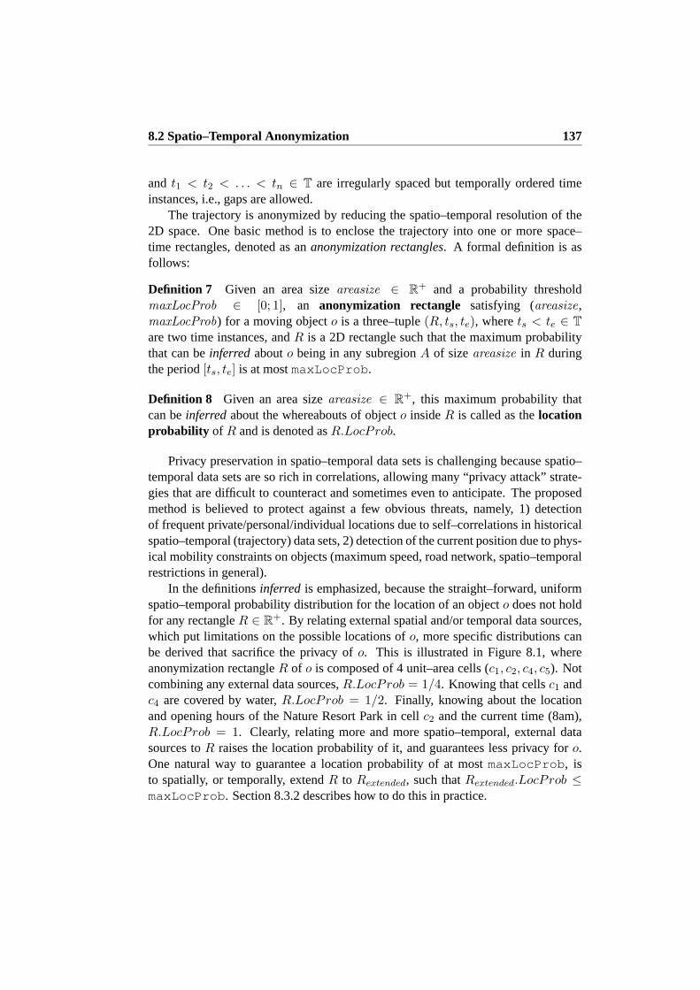
8.2 Spatio–Temporal Anonymization 137
and t1 < t2 < . . . < tn ∈ T are irregularly spaced but temporally ordered timeinstances, i.e., gaps are allowed.
The trajectory is anonymized by reducing the spatio–temporal resolution of the2D space. One basic method is to enclose the trajectory into one or more space–time rectangles, denoted as ananonymization rectangles. A formal definition is asfollows:
Definition 7 Given an area sizeareasize ∈ R+ and a probability threshold
maxLocProb ∈ [0; 1], an anonymization rectangle satisfying (areasize,maxLocProb) for a moving objecto is a three–tuple(R, ts, te), wherets < te ∈ T
are two time instances, andR is a 2D rectangle such that the maximum probabilitythat can beinferred abouto being in any subregionA of sizeareasize in R duringthe period[ts, te] is at mostmaxLocProb .
Definition 8 Given an area sizeareasize ∈ R+, this maximum probability that
can beinferred about the whereabouts of objecto insideR is called as thelocationprobability of R and is denoted asR.LocProb.
Privacy preservation in spatio–temporal data sets is challenging becausespatio–temporal data sets are so rich in correlations, allowing many “privacy attack” strate-gies that are difficult to counteract and sometimes even to anticipate. The proposedmethod is believed to protect against a few obvious threats, namely, 1) detectionof frequent private/personal/individual locations due to self–correlations in historicalspatio–temporal (trajectory) data sets, 2) detection of the current positiondue to phys-ical mobility constraints on objects (maximum speed, road network, spatio–temporalrestrictions in general).
In the definitionsinferred is emphasized, because the straight–forward, uniformspatio–temporal probability distribution for the location of an objecto does not holdfor any rectangleR ∈ R
+. By relating external spatial and/or temporal data sources,which put limitations on the possible locations ofo, more specific distributions canbe derived that sacrifice the privacy ofo. This is illustrated in Figure 8.1, whereanonymization rectangleR of o is composed of 4 unit–area cells (c1, c2, c4, c5). Notcombining any external data sources,R.LocProb = 1/4. Knowing that cellsc1 andc4 are covered by water,R.LocProb = 1/2. Finally, knowing about the locationand opening hours of the Nature Resort Park in cellc2 and the current time (8am),R.LocProb = 1. Clearly, relating more and more spatio–temporal, external datasources toR raises the location probability of it, and guarantees less privacy foro.One natural way to guarantee a location probability of at mostmaxLocProb , isto spatially, or temporally, extendR to Rextended, such thatRextended.LocProb ≤maxLocProb . Section 8.3.2 describes how to do this in practice.
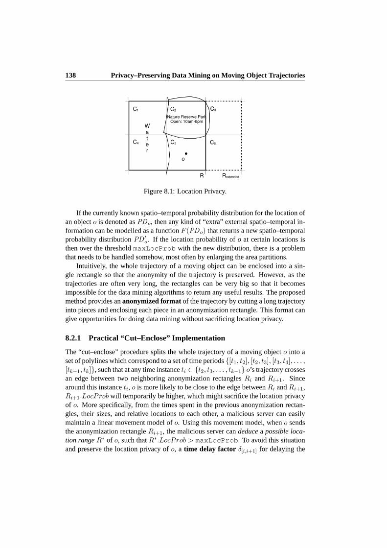
138 Privacy–Preserving Data Mining on Moving Object Trajectories
Nature Reserve ParkOpen: 10am-6pm
C1 C2 C3
C4 C5 C6
R Rextended
o
Water
Figure 8.1: Location Privacy.
If the currently known spatio–temporal probability distribution for the locationofan objecto is denoted asPDo, then any kind of “extra” external spatio–temporal in-formation can be modelled as a functionF (PDo) that returns a new spatio–temporalprobability distributionPD ′
o. If the location probability ofo at certain locations isthen over the thresholdmaxLocProb with the new distribution, there is a problemthat needs to be handled somehow, most often by enlarging the area partitions.
Intuitively, the whole trajectory of a moving object can be enclosed into a sin-gle rectangle so that the anonymity of the trajectory is preserved. However, as thetrajectories are often very long, the rectangles can be very big so that it becomesimpossible for the data mining algorithms to return any useful results. The proposedmethod provides ananonymized formatof the trajectory by cutting a long trajectoryinto pieces and enclosing each piece in an anonymization rectangle. This format cangive opportunities for doing data mining without sacrificing location privacy.
8.2.1 Practical “Cut–Enclose” Implementation
The “cut–enclose” procedure splits the whole trajectory of a moving objecto into aset of polylines which correspond to a set of time periods[t1, t2], [t2, t3], [t3, t4], . . . ,[tk−1, tk], such that at any time instanceti ∈ t2, t3, . . . , tk−1 o’s trajectory crossesan edge between two neighboring anonymization rectanglesRi and Ri+1. Sincearound this instanceti, o is more likely to be close to the edge betweenRi andRi+1,Ri+1.LocProb will temporarily be higher, which might sacrifice the location privacyof o. More specifically, from the times spent in the previous anonymization rectan-gles, their sizes, and relative locations to each other, a malicious server can easilymaintain a linear movement model ofo. Using this movement model, wheno sendsthe anonymization rectangleRi+1, the malicious server candeducea possible loca-tion rangeR∗ of o, such thatR∗.LocProb > maxLocProb . To avoid this situationand preserve the location privacy ofo, a time delay factor δ[i,i+1] for delaying the

8.2 Spatio–Temporal Anonymization 139
i i+1Ri
i+1(t )δ[i, i+1]i+1(t + )
δ[i, i+1]
R*ab
Ri+1
dc
i+1 i+2: [t , t ] :[t + ,t ]
Figure 8.2: Time Delay Factor.
sending of the anonymous rectangleRi+1 after leavingRi is introduced. The factorδ[i,i+1] can be calculated as follows. Objecto can maintain the same linear move-ment model about its own movement as the malicious server can. Hence, at anytime instancet∗ > ti, having enteredRi+1, o can calculateR∗ andR∗.LocProb.As time progresses, the size ofR∗ is monotonically increasing andR∗.LocProb ismonotonically decreasing. Hence, at some time pointts > ti, when the associatedR∗.LocProb ≤ maxLocProb it is safefor o to sendRi+1 to the server. The timedelay factor is thenδ[i,i+1] = ts − ti.
Most moving objects are confined to road networks. In the presence of roadnetworks, more sophisticated movement models are possible. Actual values for thetime delay factor have been investigated for a number of network–based movementmodels on real–world data sets in [14], but this work had a different aim, namely toaid tracking.
8.2.2 Problems with Existing Methods
To construct an anonymization rectangle for a given piece of trajectory,one naivemethod is to randomly choose a location in the vicinity of the trajectory and use thislocation as the center to build the anonymization rectangle based on a pre–definedsize. Another method, motivated from the discussion oflocation k–anonymityin theliterature [43, 44, 74], is to build the anonymization rectangle that enclose thispiecewith trajectory pieces ofk − 1 other moving objects.
However, these two methods can lead to an undesiredloss of location privacy.Sensitive locations that need to be kept private, or trajectory pieces thatlead to these,are often re–visited by the objects many times, at a similar time of day. For example,objects (users), in the evening hours return to theirhomeusing the same path (trajec-tory piece). If on different occasions the anonymization rectangles forthis trajectorypiece are constructed in anon–deterministicway, the location of the trajectory piececan be narrowed down to the intersection of these anonymization rectangles. Thisleads to an undesirable loss of privacy. In the example on Figure 8.3, object o returnsto its homeb using the same trajectory piece[a, b] on three different occasion at thesame time of the day. On the three occasions, three anonymization rectanglesRA,RB, andRC are constructed, such that they contain both the trajectory piece[a, b]

140 Privacy–Preserving Data Mining on Moving Object Trajectories
a B2B1
RC: [t , t ]C1 C2
R : [t , t ]A2A1
RA
B
b
: [t , t ]
Figure 8.3: Overlapping Area.
and the locationb. Based on the multiple visits, the location of[a, b] can be narroweddown to the small overlapping area of the anonymization rectangles.
The next section presents a grid–based solution and several methods for con-structing anonymization rectangles in adeterministicway on this grid, thereby avoid-ing the privacy loss described above. The grid–based framework alsoallows for anefficient implementation of the “cut–enclose” procedure described in Section 8.2.1.
8.3 A Grid–Based Solution
A basic method to anonymize location is to reduce the spatial resolution. Thus, in-stead of randomly constructing the anonymization rectangles or building the rectan-gles based on trajectories of other moving objects, the anonymization rectangles forall moving objects is built based on a single, pre–defined 2D grid. The followingsubsections discuss the solution in detail.
8.3.1 Grid–Based Anonymization
Denote the whole 2D Euclidean space asR2 and proceed to define an anonymization
grid and anonymization partitioning as follows.
Definition 8.3.1 An anonymization grid (briefly, a grid)G is a uniform grid ofR2
with a pre–definedO ∈ R2 as the starting point and a side lengthl. An anonymiza-
tion partitioning (briefly, a partitioning) is a set of pairwise disjoint sets of grid cellscovering all ofG.
As illustrated in Figure 8.4(a), given a starting pointO ∈ R2, the anonymiza-
tion grid (briefly, the grid)Guniformly divides the whole space into square–shapedgrid cells, each of which has side lengthl. Each grid cell has an ID value, such asc1, c2, · · · in Figure 8.4(a). Apartition of a partitioning that is defined on the grid isa set of grid cells.

8.3 A Grid–Based Solution 141
Ol
l
... ...1 2 3 4 5 6c c c c c c
partition partition partition1p p2 3
p
(a) Anonymization Grid and Partitioning.
4p 5p 6p
1t
2t3t 4t
5t
6t
7t
O
a
b d
e
fc
g
1
hp
2p 3p
(b) Anonymized Trajectory.
Figure 8.4: Grid–Based Anonymization of Trajectories.
Next, several methods for constructinganonymization partitionings based onthe anonymization grid are developed. All of the partitionings are constructed deter-ministically, thereby avoiding the privacy loss due to overlapping partitions.
Common Regular Partitioning (CRP): The simplest method is to define a single,regular partitioning that is used by all the objects. A partitioning is calledregular ifall the partitions are rectangles with side lengthsix × l andiy × l, whereix andiyare integers.
Such a regular partitioning can be seen as a coarser grid on the 2D space. Asillustrated in Figure 8.4(a), given the grid (the grid of thin lines), the partitioning(the grid of thick lines) is defined by an originO and ix = 3, iy = 3. In the ex-ample the grid cellsc1, c2, c3 belong to the partitionp1. With the grid and parti-tioning, a moving object trajectory can be transformed to a set of non–overlappinganonymization rectangles to preserve anonymity. For instance, given the trajectory〈(a, t1), (b, t2), · · · , (h, t7)〉 in Figure 8.4(b), a grid on the 2D space is built and thepartitioning on the grid is made. The partitions are denoted asp1, · · · , p6 in the fig-ure and they are non–overlapping rectangles. As described in Section 8.2.1, given thetime delay factorδ, the whole trajectory is cut into several pieces witht4−t3 = δ andt6 − t5 = δ. Then, the whole trajectory is transformed into a list of anonymizationrectangles〈(p4, t1, t3), (p5, t4, t5), (p2, t6, t7)〉.
The above described partitioning guarantees the same minimal level of privacy forall users in any region of the space. This method of partitioning is termed CommonRegular Partitioning (CRP).
Fundamental spatio–temporal data mining tasks, like finding dense spatio–tempo-ral regions, are based on simple counts or identities of the users that are present in agiven spatio–temporal region. Since in the CRP model all users report thesame set of
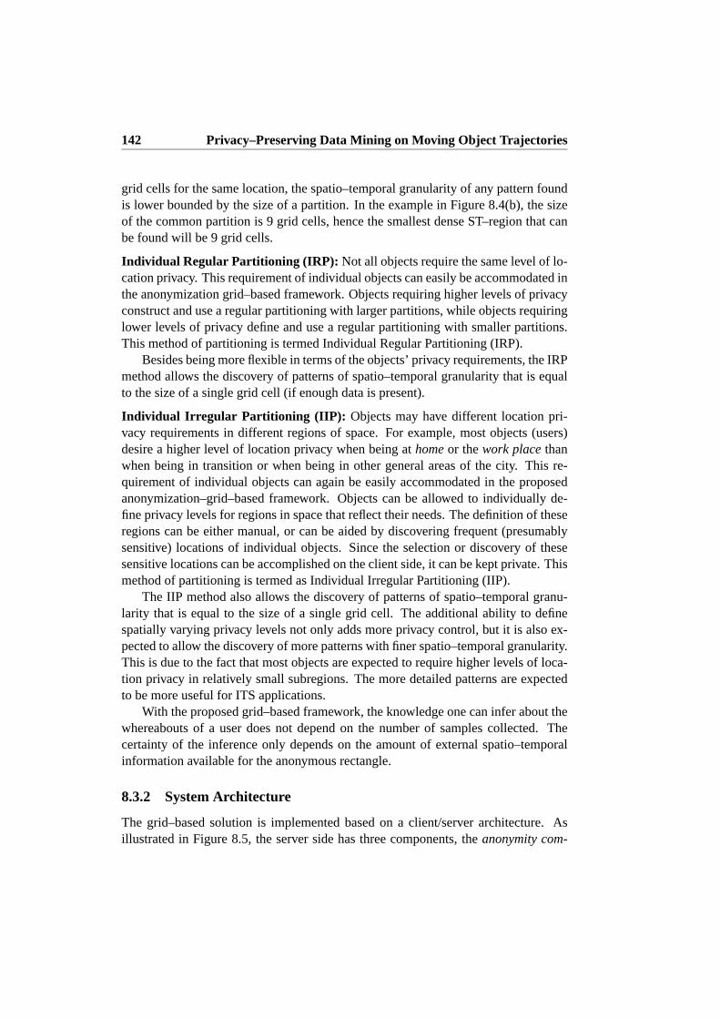
142 Privacy–Preserving Data Mining on Moving Object Trajectories
grid cells for the same location, the spatio–temporal granularity of any patternfoundis lower bounded by the size of a partition. In the example in Figure 8.4(b), thesizeof the common partition is 9 grid cells, hence the smallest dense ST–region that canbe found will be 9 grid cells.
Individual Regular Partitioning (IRP): Not all objects require the same level of lo-cation privacy. This requirement of individual objects can easily be accommodated inthe anonymization grid–based framework. Objects requiring higher levels of privacyconstruct and use a regular partitioning with larger partitions, while objects requiringlower levels of privacy define and use a regular partitioning with smaller partitions.This method of partitioning is termed Individual Regular Partitioning (IRP).
Besides being more flexible in terms of the objects’ privacy requirements, theIRPmethod allows the discovery of patterns of spatio–temporal granularity that isequalto the size of a single grid cell (if enough data is present).
Individual Irregular Partitioning (IIP): Objects may have different location pri-vacy requirements in different regions of space. For example, most objects (users)desire a higher level of location privacy when being athomeor thework placethanwhen being in transition or when being in other general areas of the city. This re-quirement of individual objects can again be easily accommodated in the proposedanonymization–grid–based framework. Objects can be allowed to individually de-fine privacy levels for regions in space that reflect their needs. The definition of theseregions can be either manual, or can be aided by discovering frequent (presumablysensitive) locations of individual objects. Since the selection or discovery of thesesensitive locations can be accomplished on the client side, it can be kept private. Thismethod of partitioning is termed as Individual Irregular Partitioning (IIP).
The IIP method also allows the discovery of patterns of spatio–temporal granu-larity that is equal to the size of a single grid cell. The additional ability to definespatially varying privacy levels not only adds more privacy control, butit is also ex-pected to allow the discovery of more patterns with finer spatio–temporal granularity.This is due to the fact that most objects are expected to require higher levelsof loca-tion privacy in relatively small subregions. The more detailed patterns are expectedto be more useful for ITS applications.
With the proposed grid–based framework, the knowledge one can infer about thewhereabouts of a user does not depend on the number of samples collected. Thecertainty of the inference only depends on the amount of external spatio–temporalinformation available for the anonymous rectangle.
8.3.2 System Architecture
The grid–based solution is implemented based on a client/server architecture.Asillustrated in Figure 8.5, the server side has three components, theanonymity com-
8.3 A Grid–Based Solution 143
ComponentTIR−treeStorage
... ...
ServerPre−definedGrids
Clients
ExpiredData
Historical Data Recent Data
Anonymity Anonymization GridComponent
Data MiningComponent
Data Mining Grid
G
G’
Cache
Paritioning 1
Client 1
Client 2AnonymizationParitioning 2
Rectangles
Anonymization
Anonymization
Figure 8.5: System Architecture.
ponentwhich defines one or more grids and communicates them to the client, thestorage componentwhich collects the anonymization rectangles sent from the clientsand stores the data on disk, and thedata mining componentwhich discovers certainpatterns and rules either directly from the incoming data stream or from the historicaldata retrieved from the storage component.
The clients are responsible for accepting an anonymization grid and developinga partitioning based on the grid. In practice, the partitioning will be made in one oftwo ways: a) the user selects among a small number of pre–computed partitioningsto find one that meets their privacy requirements, or b) the partitioning is computedby a dedicated program on the
client, based on user input about privacy requirements. Both a) and b)take avail-able background knowledge into account. The framework can also handle the pres-ence of road networks. If road networks are dense compared to the partition size,the framework can be used without modification. If not, the partitions have to beenlarged so that each partition contains enough road to get a location probability thatis comparable to those of the other partitions.
These client– and grid–specific partitionings are stored on the clients and onlyanonymization rectangles (in the form of sets of grid cells), which are computedatthe clients, are transmitted to the server. It is assumed that the client has a fair amountof storage and CPU power, but not more than what can be found in most currentlyavailable smartphones or PDAs.
Saving a partitioning at the client side does not take much space. For a regularpartitioning, where partitions form a regular grid, it is enough to store the startingpoint and the side length of the partitioning. Finding the partition that correspondsto a location is a matter of simple arithmetic. For a non–regular partitioning, wherepartitions do not form a regular grid, i.e., are of different size and/or shape, partitionscan be kept in an R–tree. Finding the partition that corresponds to a locationcan be

144 Privacy–Preserving Data Mining on Moving Object Trajectories
done by issuing a stabbing query on the R–tree for the location. The communicationcost between the clients and the server is very low since the grids can be describedwith the starting point and side lengthl of the grid, and the anonymization rectanglesonly involves a few data fields (i.e., coordinates of the client’s current partition andthe time instances).
The clients always send their current anonymization rectangle, i.e., partition, tothe server. When the anonymized data is transmitted to the server, it is stored itintwo places. To be able to perform data mining on historical data, the data is firststored in a time–interval R–tree (TIR–tree in Figure 8.5) on disk. The TIR–tree is a1–dimensional R–tree that indexes the data on the time intervals. To be able to per-form online data mining on the current data, the data is also stored in acache, with aFIFO replacement policy as follows. According to the size of the cache, when a newanonymization rectangle of a moving object arrives, either the previous anonymiza-tion rectangle of this moving object (if in the cache) or the oldest data in the cache isdeleted.
The system architecture in Figure 8.5 supports data mining on both historicaltrajectories and recent data. Each anonymization grid in the anonymity componentcorresponds to an in–memory instance of the same grid in the data mining compo-nent. For instance, the anonymization gridG in Figure 8.5 corresponds to the datamining gridG’ (it is assumed that the data mining component has enough memoryto storeG’ ). Based on this architecture, in the following, algorithms for discoveringdense ST–areason the anonymized trajectory data is presented.
8.3.3 Finding Dense Spatio–Temporal Areas
Discovering dense areas is one of the most common topics for spatial and spatio–temporal data mining. Existing research work has explored density clustering [20],spatio–temporal dense area discovery [95], and density queries [59]. For dense areadiscovery on the anonymized trajectory data, the most basic operation is to find thosegrid cells that contain a large amount of moving objects during specified time inter-vals. In the anonymized format, objects are present in a grid cell with someprob-ability only. Hence, atime interval probabilistically dense spatio–temporal areaquery, or dense ST–area queryfor short is proposed, which can be seen as a basic,atomic operation for advanced dense area mining algorithms over the anonymizationgrid. Such advanced and complex data mining algorithms can be made by assemblingthis operations with other basic query types.
Specifically, suppose a moving objecto corresponds to a partitionP on a givenanonymization gridG, a partition cellp ∈ P containso’s trajectory during timeinterval [ts, te], andp includes grid cellsc1, c2, . . . , ck. p is used as the anonymiza-tion rectangle foro’s trajectory and each grid cellci ∈ p has the location proba-bility co
i .LocProb = 1/k for o at any time instance during[ts, te]. Let Oci be the

8.3 A Grid–Based Solution 145
set of moving objects whose anonymization rectangles include the grid cellci in atleast one time instance during the time interval[ts, te]. Thenci.count = |Oci | andci.prob =
∑
o∈Oci coi .LocProb/|Oci |. Intuitively, ci.count is themaximumnum-
ber of objects thatcan be insideci during [ts, te], while ci.prob is theaveragelo-cation probability of the objects that can be insideci during [ts, te]. Consequently,ci.prob×ci.count is theexpectednumber of objects insideci during[ts, te]. Further-more, thepattern certaintyci.cert =
∏
o∈Oci coi .LocProb is defined as the probabil-
ity of actuallyhavingci.count number of moving objects inside ofci during[ts, te].A grid cell ci is said to beprobabilistically denseduring [ts, te] if ci.count ≥
min count andci.prob ≥ min prob , for some given threshold valuesmin countandmin prob . Thus, thedense ST–area queryis formulated as follows:
Definition 8.3.2 A dense ST–area queryQ = ([ts, te], min count , min prob )retrieves all the grid cells whose correspondingcount andprob values during[ts, te]are greater than or equal tomin count andmin prob , respectively.
To process a dense ST–area query, the first step is to compute thecount andprobvalues for each grid cellci for the specified time interval[ts, te]. Based on the systemarchitecture in Figure 8.5, a range query over the TIR–tree needs to be issued to findall the anonymization rectangles whose time periods have intersections with[ts, te].Results of the range query are used to fill in thecount andprob values for each cellci of the data mining gridG’ . Then the set of dense ST–grid cells is:
D = ci : ci.count ≥ min count ∧ ci.prob ≥ min prob
During the query time interval[ts, te] a moving object can leave and later reenter agiven grid cellci. To avoid counting such an object multiple times forci, a hash arrayof object IDs is maintained and values forci.count and ci.prob are only updatedwhen an object ID is encountered forci for the first time. If only approximate countsare considered, these can be more effectively obtained using the methodsfrom [90].
As it will be seen in Section 8.4, the cut–off criteria for dense areas presentedabove is in some cases not strict enough, thus generating too many dense areas (falsepositives). To remedy this, the alternativesteepest slopecut–off criteria is introduced,which is calculated by first sorting the expected counts for dense areas passing thefirst criteria in descending order, finding the deltas between any two consecutive val-ues, and making the cut–off where the (negative) delta is the smallest, i.e., where the“slope” is steepest.
The above method is simple to implement but can not discover all the dense areasthat have the size of a single grid cell. As illustrated in Figure 8.6(a), grid cellsc1, c2, c3, c4 have several moving objects (big dots in the figure) and the thresholdmin count = 4. None of the four cells are reported as dense since thecountvalueof each is less than 4.
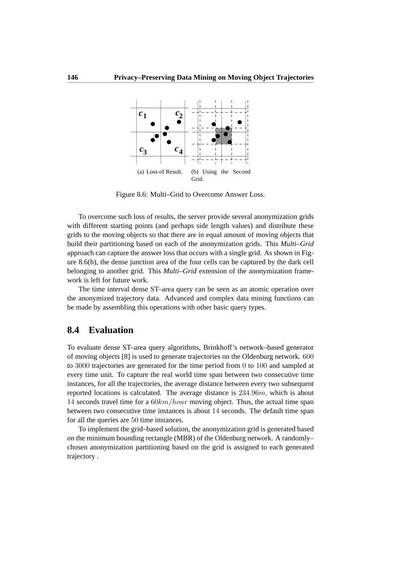
146 Privacy–Preserving Data Mining on Moving Object Trajectories
c
c1 c2
4c3
(a) Loss of Result. (b) Using the SecondGrid.
Figure 8.6: Multi–Grid to Overcome Answer Loss.
To overcome such loss of results, the server provide several anonymization gridswith different starting points (and perhaps side length values) and distribute thesegrids to the moving objects so that there are in equal amount of moving objects thatbuild their partitioning based on each of the anonymization grids. ThisMulti–Gridapproach can capture the answer loss that occurs with a single grid. As shown in Fig-ure 8.6(b), the dense junction area of the four cells can be captured by the dark cellbelonging to another grid. ThisMulti–Grid extension of the anonymization frame-work is left for future work.
The time interval dense ST–area query can be seen as an atomic operation overthe anonymized trajectory data. Advanced and complex data mining functions canbe made by assembling this operations with other basic query types.
8.4 Evaluation
To evaluate dense ST–area query algorithms, Brinkhoff’s network–based generatorof moving objects [8] is used to generate trajectories on the Oldenburg network. 600to 3000 trajectories are generated for the time period from0 to 100 and sampled atevery time unit. To capture the real world time span between two consecutive timeinstances, for all the trajectories, the average distance between every two subsequentreported locations is calculated. The average distance is234.96m, which is about14 seconds travel time for a60km/hour moving object. Thus, the actual time spanbetween two consecutive time instances is about14 seconds. The default time spanfor all the queries are50 time instances.
To implement the grid–based solution, the anonymization grid is generated basedon the minimum bounding rectangle (MBR) of the Oldenburg network. A randomly–chosen anonymization partitioning based on the grid is assigned to each generatedtrajectory .

8.4 Evaluation 147
The default grid is a40× 40 partitioning on the MBR of the Oldenburg network.Based on the Oldenburg network data, the size of each grid cell is589m × 672.9m.In the experiments, the grid partitioning is also tuned from20 × 20 to 50 × 50 toobserve the performance. The three policies are applied on the trajectories with theanonymization grid. To implement the CRP policy, two fixed partitionings are made,where each user has2 × 2 or 4 × 4 grid cells. In the IRP policy, every user partitioncontains at most4×4 grid cells. In the IIP policy, each moving object is set to use theanonymization partition (each partition contains at most4 × 4 grid cells) that coversthe start location of the moving object. After the object is out of this partition, it usesthe lowest level of privacy so that each partition equals to a grid cell.
The experiments focus on evaluating the accuracy of the algorithms, i.e., theamount of false positives and false negatives. A false negative, is the error of notfinding a pattern that does exist in the data. A false positive, is the error offinding a“pattern” that does not exist in the data. To compare the algorithms, the algorithmsare also applied on an ideal case, where the partitioning of every user equals theanonymization grid, and use the results of this case as the evaluation target. Supposethe actual amount of dense grid cells isD, the number of false positivesP and falsenegativesN are collected for every algorithm and the ratio between these values andD are reported, called thefalse positive rate(FPR) andfalse negative rate(FNR), re-spectively. The choice of these measures over the precision and recallmeasures usedin information retrieval is because of conceptual simplicity. In the present case differ-ent kinds of errors are related to the same reference set (D), whereas in informationretrieval the same set of correctly retrieved patterns are related to the setof all truepatterns (recall) and to the set of retrieved patterns (precision). Hence, more accurateresults are characterized by lower error rates rather than by higher recall and preci-sion. However, it holds that Recall=1-FNR and Precision=(1-FNR)/(1-FNR+FPR).
In the experiments, thecountandprobvalues are tuned to observe the amount offalse positives and false negatives. Experiments have also been conducted to test theeffect of grid size, time span and amount of trajectories on the accuracy.As seen inFigure 8.7(a) to Figure 8.7(e), there are very few false negatives andthe amount offalse positives grows in certain cases. In particular, based on Figure 8.7(a), with thegrowth ofcountvalues, more false positives appear. With the experiment on theprobvalue (Figure 8.7(b)), it is possible to reach an optimal situation by tuning thisprobvalue for each policy. For instance, the IRP policy has fewer false positives whenprob= 0.1 and so has IIP whenprob= 0.3. An observation from Figure 8.7(c) is thatthe amount of false positives grows with the grid size. The explanation for this is asfollows. As the grid becomes denser, there are fewer really dense grid cells, but theamount of dense cells found through the three policies does not decrease very much,so the reported ratio value becomes larger. Figure 8.7(d) and Figure 8.7(e) show that
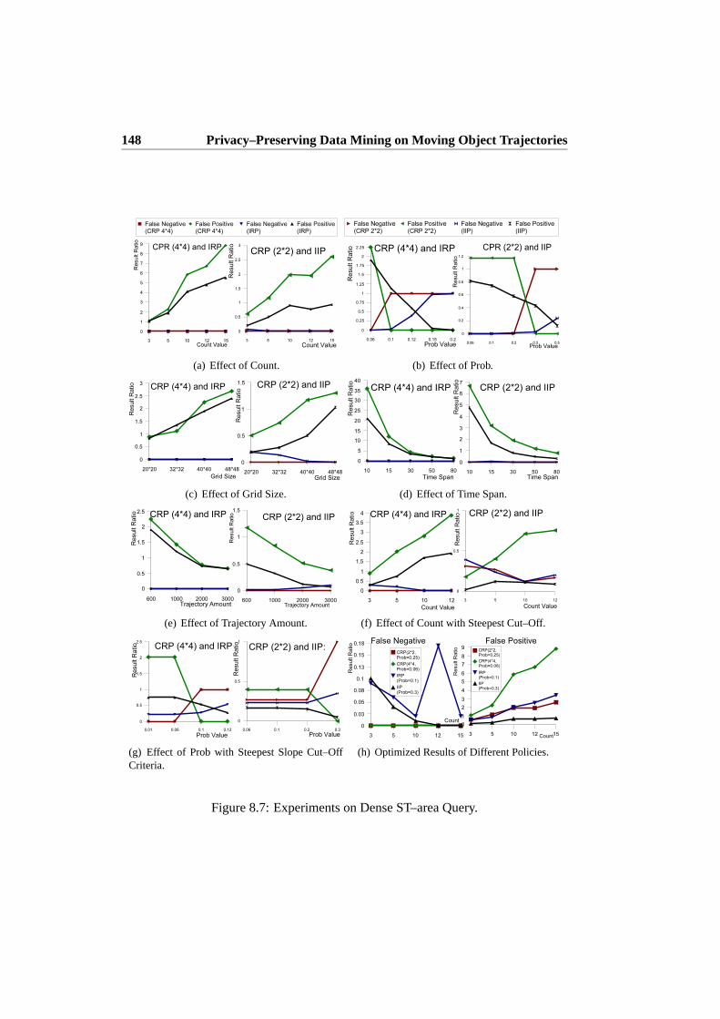
148 Privacy–Preserving Data Mining on Moving Object Trajectories
(a) Effect of Count. (b) Effect of Prob.
(c) Effect of Grid Size. (d) Effect of Time Span.
(e) Effect of Trajectory Amount. (f) Effect of Count with Steepest Cut–Off.
(g) Effect of Prob with Steepest Slope Cut–OffCriteria.
(h) Optimized Results of Different Policies.
Figure 8.7: Experiments on Dense ST–area Query.

8.5 Conclusions and Future Work 149
the increase of the time span and the amount of trajectories reduces the amount offalse positives for all the policies.
To test how the steepest slope cut–off criteria influences the algorithms, thecountandprobvalues are tuned to observe the amount of false positives and false negativeson the different policies. As illustrated in Figure 8.7(f) and Figure 8.7(g),the cut–offcriteria decreases the amount of false positives but, compared to the same settings inFigure 8.7(a) and Figure 8.7(b), brings more false negatives. Thus, considering allthe parameters for the three policies, the following are therecommendationsettingsfor the dense ST–area query:
The IIP is the most effective policy for doing dense ST–area query with privacyprotection. The second and third best choice is the CRP policy with2×2 partitioningand the IRP policy. For all the policies, certain optimal situation on the amountof false positives and false negatives can be reached by tuning the prob value. Toincrease the time span and amount of trajectories will improve the performance ofall approaches.
Based on therecommendation, an experiment is conducted to compare the dif-ferent policies with their optimal settings. In this experiment, the amount of trajec-tories is increased to1000 and optimalprob values are used for each policy. Fig-ure 8.7(h) presents the results. The CRP policy with each partition containing2 × 2cells and the IIP policy shows the most promising performance. These two policiesguarantee a precision level that makes them useful for most applications.
8.5 Conclusions and Future Work
Motivated by the possible loss of location privacy for LBS users, this paper proposeda general grid–based framework that allowed user location data to be anonymized.Thus, privacy is preserved, but interesting patterns could still be discovered. Theframework allowed users to specify individual desired levels of privacy and devel-oped three policies for implementing that. Privacy–preserving methods werepro-posed for a core data mining task, namelyfinding dense spatio–temporal regions. Anextensive set of experiments evaluated the methods and showed that the frameworkstill allowed most patterns to be found, even when privacy was preserved.
Future work will be along three paths. First, theMulti–Grid approach will be fur-ther investigated as it offers a direction for getting more detailed data mining resultswithout violating the privacy. Second, in addition to the CRP, IRP and IIP policies,it is possible to develop more policies for creating anonymization rectangles suitablefor different real world situations. Third, since the grid–based solutioncan be seen asa simple and general framework for privacy preserving data mining on moving objecttrajectories, hance the framework is planned to be extended to support more kinds ofspatio–temporal data mining algorithms.

Chapter 9
Privacy–Preserving TrajectoryCollection
Context awareness is one of the most important features of user–friendly Location–Based Services (LBS). To support context awareness in LBSes, real location data ofmobile users has to be collected so that spatio–temporal patterns can be extracted bydata mining methods. This brings a new conflict of interest: the data mining meth-ods want precise location data, while the mobile users want to protect their privacyby not disclosing their exact movements (trajectories). To resolve the conflict, thepaper first formally defines novel location privacy requirements. Then, it presentsa system for privacy–preserving trajectory collection that meet these requirements.The system is composed of an untrusted server and clients communicating in a P2Pnetwork. Location data is anonymized in the system using data cloaking and dataswapping techniques. The proposed system is empirically evaluated on realistic sim-ulated movement data and is found to be effective under reasonable conditions andprivacy/anonymity settings.
9.1 Introduction
The convergence among mobile services and positioning technologies paves the wayfor a range of new, innovative services, which are commonly referredto as Location–Based Services (LBSes). Emergence of LBSes creates a demand for novel data man-agement technologies to efficiently support new data types, operations, and work-loads. Context awareness, as one of the most important features of LBSes, is inte-grated in mobile devices so that these devices have information about the circum-
151

152 Privacy–Preserving Trajectory Collection
stances under which they operate and can react accordingly. To support contextawareness in LBSes, real location data of mobile users has to be collected so thatspatio–temporal patterns can be extracted by data mining methods. This bringsanew conflict of interest: the data mining methods want precise location data, whilethe mobile users want to protect their privacy by not disclosing their exactmove-ments. The following example describes the problem scenario.
A large shopping center wants to do data mining on the activities of customers inbusiness hours. One type of customer activity is where and when customers were inthe shopping center. To collect the activity information, it is assumed that a position-ing system such as GPS, radiolocationing, or RFID detects the locations of the cus-tomers’ mobile phones. Customers locations are recorded in the phones andsent toa central server. The central server then collects and analyzes the customers’ spatio–temporal location data. However, it is a violation of privacy foranyone, includingthe server, to know exactly when and where an individual customer was.Thus, a so-lution that can collect the activity information from mobile phones without exposingthe privacy of users is desirable.
Movements of mobile users are often modelled as trajectories in 2D space. Datamining on the trajectory data has many applications, not only in LBSes, but alsointelematics and Intelligent Transportation System (ITS). Methods have beenproposedto extract patterns, such as dense regions [47, 59] and frequent routes [32] from thetrajectory data. An existing solution for protecting the location and trajectory datain LBSes is to anonymize the users’ location data by decreasing the spatio–temporalresolution of the locations. After this “anonymization” step, the exact locationdatabecomes a set of spatio–temporal rectangles. Although such ambiguity protects themobile users’ privacy, it also reduces the accuracy of the data mining results.
Motivated by these observations, this paper defines new privacy requirements forlocation/trajectory data and presents a system for collecting mobile users’ trajectorydata in a privacy–preserving manner. Compared to existing solutions, the proposedsystem does not require trusted components, yet it protects the privacyof mobile usersand preserves the accuracy of data mining by keeping the spatio–temporaldata in-tact. The proposed solution assumes that clients on mobile phones can communicatethrough a wireless P2P network. The process of trajectory collection is divided in fivestages as follows. First, in theclient registrationstage, a group ofk clients obtainspermission and parameters from the server for executing thetrajectory sampling andanonymization–, the trajectory exchange–, and thedata reportingstages in a multi-threaded fashion. In thetrajectory sampling and anonymizationstage, clients recordtheir private trajectories and generate a set ofk “cloaking” trajectories to anonymizetheir actual trajectory. In thetrajectory exchangestage, clients exchange sets ofkpartial trajectory pieces with other clients in the P2P network. Finally, in thedatareportingstage, clients send anonymous partial trajectory pieces to the server. In the

9.2 Related Work 153
meanwhile, in thedata summarizationstage, the server continuously listens to datareports from clients, assembles the trajectory pieces and filters out the “cloaked” tra-jectories. An extensive experimental evaluation, based on realistic simulatedtrajec-tory data, shows that the proposed approach is effective under reasonable conditionsand privacy/anonymity settings.
The contributions of this paper are believed to be as follows. First, the paperadapts and combines previous general privacy definitions to derive privacy defini-tions of various strengths for location data. More specifically, the paper definesk–anonymity, α–diversity, requiring spatial diversity, andk–α–anonymityfor locationdata. Second, the paper proposes a complete system, including algorithms and imple-mentation details, for thelosslesscollection ofexacttrajectories of moving objects.The proposed system does not require trusted components, yet it guarantees at leastk–anonymityin all parts of the collection process. The proposed system isscalableas the process of anonymization is performed in a distributed fashion by clients inter-acting via a P2P network. The security of the proposed system is evaluatedand thesystem is found to be robust against a wide variety of attacks by malicious clients ora malicious server (if it is hacked). In particular, the system is shown to guarantee theanonymity of the client data on both the client and the server side and any time duringtransmission in the air. Finally, the paper demonstrates through an extensiveempiri-cal evaluation that the proposed system is effective under reasonableconditions andprivacy/anonymity settings.
The rest of this paper is organized as follows. Section 9.2 explores related work.Section 9.3 discusses the basic concepts relating to location privacy. Section 9.4 de-scribes the proposed solution in detail, while Section 9.5 analyzes the privacy guaran-tee of the solution. Section 9.6 presents the empirical evaluation. Finally, Section 9.7concludes and points out future directions for research.
9.2 Related Work
The topic of privacy preserving data mining [4] has appeared due to the concern ofprotecting privacy in the data collection and dissemination steps of data mining pro-cess. The database and data mining research communities have been very active in thediscussion of privacy–preserving data mining. Important techniques include pertur-bation, condensation, and data hiding with conceptual reconstruction. The paper [96]presents a good review of these techniques. The techniques behind the proposed so-lution follow the spirit of two common strategies used for privacy–preserving datamining, namely datacloakingand dataswapping.
Several papers [12, 43, 44, 74] have addressed the topic of privacy–preservinglocation–based services. These papers assume an architecture wherea piece of trustedmiddleware, often termed ananonymizer, exists between mobile users and LBS
154 Privacy–Preserving Trajectory Collection
servers. Based on the query requests from mobile users, the anonymizer constructsanonymity rectangles that include the locations ofk users and sends a query to theLBS server with this rectangle as the location. The LBS server returns a supersetof the results and final results are filtered by the anonymizer and sent back to eachLBS user. Compared to these papers, the architecture proposed in this paper does notrequire a piece of trusted middleware. In fact, the anonymization process isdone atthe client side through the P2P network.
The proposed solution is focused on the data modification of the collected userdata. In the existing papers, the data modification techniques used in the anonymizerare based on the ideas of aggregation and perturbation. In particular, papers [43, 44]extend thek–anonymity model [89] in relational databases to aggregate the locationsof k mobile users so that the location of an individual user is not distinguishable.Theadaptive location anonymizer discussed in [74] uses a grid–based pyramid structureto put the exact location of mobile users into cloaking rectangles made of grid cells.Paper [12] suggests a data model to augment uncertainty to location data, and proposeimprecise queries that hide the location of the query issuer and yield probabilisticresults. Compared to these existing techniques, the architecture in this paperdoes notuse an anonymizer but distributes the anonymization step to client–side computationand communication. In previous work [35], a grid–based framework forprivacy–preserving data collection is proposed. This framework protects the privacy of mobileusers but also blurs the exact collected spatio–temporal locations which influencesthe accuracy of data mining results. To keep the quality of the collected data withoutviolating the privacy, this paper proposes a novel data modification approach based onthe idea ofswapping[96]. Similar to the architecture described in [13], the presentsolution assumes the existence of a P2P network. As it will be shown later, thetechnique behind the present solution, compared to the aggregation and perturbationtechniques, does not introduce any ambiguity into the location data, which ultimatelyguarantees the precision and quality of the data mining results.
9.3 Preliminaries
For the simplicity of the discussion, assume that the time domainT is totally orderedand use the non–negative numbers as the time domain. Denote each moving object asadata item. A data item is modelled as a two tupledi = (id, S) whereid is the iden-tity attribute value of the data item andS is the trajectory ofdi. It is modelled as a se-quence of tuplesS = 〈(loc1, t1), . . . , (locn, tn)〉 whereloci ∈ R
2 (i = 1, . . . , n) arelocations, andt1 < t2 < . . . < tn ∈ T are (possibly irregularly spaced) temporallyordered time instances. Next, atrajectory pieceis defined as a subset of a trajectoryordered on the time domain. For instance,S1 = 〈(loc1, t1), (loc2, t2), . . . , (lock, tk)〉andS2 = 〈(lock+1, tk+1), (lock+2, tk+2), . . . , (locn, tn)〉 are two trajectory pieces

9.3 Preliminaries 155
of S = 〈(loc1, t1), . . . , (locn, tn)〉. For a given data itemdi = (id, S), bothdi1 =(id, S1) anddi2 = (id, S2) (with di1.id = di2.id = di.id) can represent part of thetrajectory ofdi. di1 anddi2 are calledpartial data items, or itemsfor short.
A simple way of protecting trajectories of mobile users is to hide the identity ofusers in the data items. Specifically, given a data item(id, S), by hiding the identity(e.g., encoding theid value), it is impossible to deduce the mobile user from theidvalue. However, an adversary can still study if a given data item corresponds to aspecific user by cross–referencing from other public information about the user (e.g.,work address, home address, etc.). If a trajectoryS covers many relevant addressesof a user, it is possible that the data item(id, S) describes the trajectory of this user.
As described in related works, a dominant technique for protecting the spatialand spatio–temporal locations of users is to keep each user’s locations anonymousamong a set of other users. This so–calledk–anonymitytechnique is also applicableto protect the trajectories (and, trajectory pieces) of mobile users. The followingdefines thek–anonymity of data items.
Definition 9 (k–anonymity of data items) For a set of moving objectsMO =o1, . . . , om and a set of data itemsDI = (id1, S1), . . . , (idn, Sn), m ≤ n whereid1, . . . , idn are encoded identity values andS1, . . . , Sn are trajectory pieces, themoving objects and the data items are said to preservek–anonymityif both of thefollowing conditions are true:
1. For any objecto, there are at leastk data items(id′1, S′1), . . . , (id′k, S
′k) that
correspond to this object with equal probability.
2. For any data item(id, S), there are at leastk objectso′1, . . . , o′k that correspond
to the data item with equal probability.
Thek–anonymity of data itemspreserves the anonymity when an adversary matchestrajectories to specific moving objects. However, in an extreme case, when the tra-jectories of moving objects are almost identical (e.g., cars moving on the same roadsin the road network), the spatial and spatio–temporal privacy of these objects is stillexposed as the possible locations of each object can be narrowed downto the com-mon parts of the trajectories. To improve the protection of the trajectories of movingobjects, as in the general privacy protection framework [69], it is necessary to re-quire that these trajectories possess a certain spatial diversity. Hence,the definitionof α–diversityis introduced in the following.
Definition 10 (α–diversity of data items) For a set of data itemsDI = (id1, S1), . . . ,(idn, Sn) whereid1 6= id2 6= . . . 6= idn, a given thresholdα, these data items pre-serveα–diversityif AREA(MBR(S1, . . . , Sn)) ≥ α, whereMBRis the minimumbounding rectangle ofS1, . . . , Sn andAREAreturns the area size of an MBR.
156 Privacy–Preserving Trajectory Collection
Next, combining the definitions ofk–anonymityandα–diversity, a more strictsetting to protect the privacy the data items is presented, namely thek–α–anonymity.
Definition 11 (k–α–anonymity of data items) For a set of moving objectsMO =o1, . . . , om and a set of data itemsDI = (id1, S1), . . . , (idn, Sn), k ≤ m ≤ nthat preservek–anonymity, and a threshold valueα, the moving objects and dataitems satisfyk–α–anonymityif the following condition is true. For anyk data items(id′1, S
′1), . . . , (id
′k, S
′k) ∈ DI, these data items preserveα–diversity.
Thek–α–anonymityis a more restrictive requirement to preserve the privacy ofmoving object trajectories. In particular, given anα value, it is not guaranteed thatthek–α–anonymitycan be achieved by the sets ofk–anonymousmoving objects anddata items. For example, consider a group ofk drivers living in the same suburb areaand working in the city center. The set ofk drivers and their corresponding set oftrajectories isk–anonymous. However, since it is very likely that the trajectories ofthese drivers are quite alike, the MBR of these trajectories is likely to have anareathat is smaller than any reasonable value forα. Hence, the set of drivers and theircorresponding set of trajectories do not satisfyk–α–anonymityfor any reasonablevalue ofα. The diversity of spatial and spatio–temporal locations is decided by themobile users.
The aim of the herein proposed data collection solution is to preserve anonymityof data items (or partial data items) in any set of data being stored, transmitted orcollected in the system. As described later, the solution preservesk–anonymityinall sections of the system and achievesα–diversityor k–α–anonymityin the partsthat are more vulnerable to privacy threats. In the following details of the proposedsolution are described.
9.4 Solution
The proposed solution is for a scenario in which users have mobile phonesequippedwith a positioning device and these mobile phones can communicate with each otherthrough a P2P network. Such a scenario is very reasonable in real–world applicationsthat are fuelled by technical advances such as the development of smartphones withembedded GPS devices and the widespread availability of WiFi and Bluetooth,andthe scalability and robustness of the P2P application design paradigm. Assuming thatthe solution aims to preservek–anonymity, α–diversityandk–α–anonymity(with kandα as concrete values) in all aspects of trajectory data collection, the followingsubsections describe the architecture of the proposed system and its detailed privacypreserving procedures.
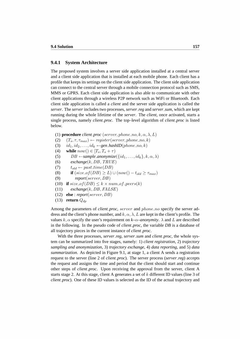
9.4 Solution 157
9.4.1 System Architecture
The proposed system involves a server side application installed at a central serverand a client side application that is installed at each mobile phone. Each client has aprofile that keeps its settings on the client side application. The client side applicationcan connect to the central server through a mobile connection protocol such as SMS,MMS or GPRS. Each client side application is also able to communicate with otherclient applications through a wireless P2P network such as WiFi or Bluetooth. Eachclient side application is called aclient and the server side application is called theserver. Theserverincludes two processes,serverregandserversum, which are keptrunning during the whole lifetime of theserver. Theclient, once activated, starts asingle process, namelyclient proc. The top–level algorithm ofclient proc is listedbelow.
(1) procedureclient proc (server, phone no, k, α, λ, L)(2) (Ts, τ, τmax) ← register(server, phone no, k)(3) id1, id2, . . . , idk ←genhashID(phone no, k)(4) while now() ∈ [Ts, Ts + τ)(5) DB ←sampleanonymize(id1, . . . , idk, k, α, λ)(6) exchange(k,DB ,TRUE )(7) told ← past time(DB)(8) if (size of(DB) ≥ L) ∪ (now() − told ≥ τmax)(9) report(server,DB)(10) if size of(DB) ≤ k × num of peers(k)(11) exchange(k,DB ,FALSE )(12) else: report(server,DB)(13) return Qdp
Among the parameters ofclient proc, server andphone no specify the server ad-dress and the client’s phone number, andk, α, λ, L are kept in the client’s profile. Thevaluesk, α specify the user’s requirement onk–α–anonymity. λ andL are describedin the following. In the pseudo code ofclient proc, the variableDB is a database ofall trajectory pieces in the current instance ofclient proc.
With the three processes,serverreg, serversumandclient proc, the whole sys-tem can be summarized into five stages, namely: 1)client registration, 2) trajectorysampling and anonymization, 3) trajectory exchange, 4) data reporting, and 5)datasummarization. As depicted in Figure 9.1, at stage 1, a client A sends a registrationrequest to the server (line 2 ofclient proc). The server process (serverreg) acceptsthe request and assigns the time and period that the client should start and continueother steps ofclient proc. Upon receiving the approval from the server, client Astarts stage 2. At this stage, client A generates a set ofk different ID values (line 3 ofclient proc). One of these ID values is selected as the ID of the actual trajectory and

158 Privacy–Preserving Trajectory Collection
Client C
5. Data Summarization
1. Client Registration
Server2. Trajectory Sampling
and Anonymization
3. Trajectory Exchange
Client ARequest
Approval
Server Side Client Side
Client B
4. Data Reporting
Figure 9.1: System Architecture.
the others are used as the ID values of synthetic trajectories (explained later). Thesynthetic trajectories with these ID values are called thecloaking trajectory data.Client A begins to record its trajectory data and generate the cloaking trajectory data(line 5 of client proc). The parameterλ of client proc specifies the time interval forcutting the collected trajectory and the cloaking data into trajectory pieces. Thepa-rameterC is used in thetrajectory sampling and anonymizationstage to specify howthe synthetic trajectories should be generated. Then, at stage 3, throughthe P2P net-work, client A communicates with clients B and C to exchange the anonymized data(line 6 of client proc). The trajectory sampling and anonymizationand trajectoryexchangesteps are kept running until the period specified by the server is reached(the while–loop ofclient proc). At stage 4, when aclient has reached its storagelimit (specified by the parameterL of theclient proc) or if it has a very “old” pieceof trajectory data, this client reports its data to the server (line 9 ofclient proc). Thestage ofdata reportingalso happens when clients are at the end of the activation pe-riod (lines 10–12 ofclient proc). In Figure 9.1, clients A, B choose to transmit theircollected data to other peers in the P2P network (line 11 ofclient proc) and client Csends its the data to the server (line 12 ofclient proc). Finally, at stage 5, the serverprocessserversumsummarizes the data from the clients, filters out the synthetic tra-jectory data and computes the real trajectory data. The next subsections describesdetails of these stages.

9.4 Solution 159
m=max(k , ..., k )
... ...(A , k )nn
(A , k )11
Client Am
Client A1
Client A2
Client An
(A , k )11
(A , k )22
(A , k )mm
(A , k )nn
sτ τmax(T , , )
sτ τmax(T , , )
sτ τmax(T , , )
sτ τmax(T , , )
... ...(A , k )m m
FIFO Buffer
... ...
First m tuples
... ...
Server Clients
m1
Figure 9.2: Client Registration.
9.4.2 Client Registration
Each client must start with theclient registrationstep. At this step, the functionregis-ter(server, phone no, k) sends a registration request message to theserver, togetherwith its phone number and thek value.
At the server side, when the processserverreg receives a request message, itsaves the request in a FIFO buffer. This process also maintains the maximalk valueof all these requests, denoted askmax. When the FIFO buffer haskmax elements, theserverregprocess sends out messages to each of the firstkmax registration requests,removes all elements from the buffer, and setskmax = 0. As illustrated in Figure 9.2,each of the clientsA1, . . . , An sends a message withphone no, k. When the amountof tuples in the buffer is equal tokmax, i.e., m = max(k1, k2, . . . , km), the serversends approval messages to thesem mobile phones. An example approval messagecan beTs, τ, τmax whereTs denotes the time that the client should continue withother steps ofclient proc, τ describes how long each client should keep running thesesteps, andτmax specifies a time period that will be used in theclient proc to start thedata reportingstage. In reality, the value ofτ reflects the average time period that aclient is active, e.g., the average time span that customers spend at a shopping center.Without loss of generalityτ is a static threshold value stored at the server. However, itis possible to implementτ as a dynamic value. For instance, each client can send theregistration request message with an anticipated active time period. Then the server

160 Privacy–Preserving Trajectory Collection
can organizek clients into a group if they have similar active time periods and usethe maximal of these time periods asτ for clients of this group.
9.4.3 Trajectory Sampling and Anonymization
At this stage, a set ofk different ID values are generated at the client. To ensure thatthe k values are unique among the other ID values generated at different instancesof the clients, in the functiongenhashID (line 3 of client proc), the Secure HashAlgorithm (SHA) [88] is used to generate the ID values. The input to the SHAfunction is a combination of the phone numberphone no and the current timestamp.If the input values are unique, based on the properties of the SHA functions, thegenerated hash values are also unique among all instances of the clients. Althoughrecent research [99] has found an attack in which two separate messages could befound that deliver the same SHA–1 hash using269 operations, stronger versions ofSHA, such as SHA–256 and SHA–512, can be used to further improve thesecurityof the hash function.
Take client A in Figure 9.1 as an example. Suppose thesek ID values generatedat client A areid1, id2, . . . , idk. Client A randomly decides one of thesek values asthe ID value of the collected trajectory. In thesampleanonymizefunction started atthe trajectory sampling and anonymizationstage (line 5 ofclient proc), without lossof generality,id1 is used for the collected trajectory, denoted byS1, and the other IDvalues are used for the synthetic trajectoriesS2, . . . , Sk. This function collects thetrajectory of the client and adds synthetic trajectories for anonymizing the collecteddata. The pseudo code is listed in the following.
(1) proceduresampleanonymize(id1, . . . , idk, k, α, λ, C)(2) S1 ←sampletrajectory()(3) S2, . . . , Sk ← gen trajectory(k, α, C)(4) at everyλ interval:(5) for eachSi, i = 1, . . . , k(6) S′
i ←get piece(Si, now() − λ, now())(7) n1 ← 2z; n2, . . . , nk ← 2z + 1 : z ∈ Z
+
(8) add(id1, S′1), . . . , (idk, S
′k) to DB
(9) return DB
In this algorithm, while the trajectory dataS1 is being sampled by thesampletrajectoryfunction (line 2), client A also generatesn−1 synthetic trajectoriesS2, . . . , Sk (func-tion gen trajectory in line 3). Thesampletrajectory function collects the actual lo-cations at every unit time instance. Then, at every time intervalλ, client A appliestheget piecefunction on the trajectoriesS1, . . . , Sk and gets the trajectories piecesfor time [now() − λ, now()). The intervalλ is one or more time units and functionnow() gives the current unit time instance.

9.4 Solution 161
λ
1 S3 S2
1S’
1p
3S’ 2S’
2p
3p
1q 2
q3
q
x
t
y
now()
S
Figure 9.3: Theget pieceFunction.
As illustrated in Figure 9.3, theget piecefunction cuts the pieces during timeinterval[now()−λ, now()) on each of the three trajectoriesS1, S2, S3. The trajectorypieces between(p1, q1), (p2, q2), (p3, q3) are denoted byS′
1, S′2, S′
3. Tuples(id1, S′1),
(id2, S′2), (id3, S
′3) are added toDB (line 8). The tuple(id1, S
′1), whereid1 is the ID
value of the actual trajectoryS1 andS′1 is obtained fromS1, is called thereal data
item. The other data items(id2, S′2), . . . , (idk, S
′k), are calledcloaking data items.
To distinguish the real data item among all the data items, the client generatesan even number of copies of the real data item and an odd numbers of copies of thecloaking items. The idea of having copy amounts of the data items with differentparity is to hide the real data items in exchanges between clients, but to be able toidentify them at the server. Specifically, given an instance ofk data items, one withan even andk − 1 with an odd number of copies, it is impossible for a client holdingsome, but not necessarily all, copies of a data item to decide whether the dataitemis real or cloaked. Accordingly, on line 7, one even (n1) andk − 1 odd(n2, . . . , nk)copy amounts are calculated; each valueni determines the number of copies of a dataitem (idi, S
′i). Finally, copies of the data items(id1, S
′1), . . . , (idk, S
′k) are added to
the trajectory databaseDB (line 8).In thegen trajectory function, synthetic trajectoriesS2, . . . , Sk are generated in
two steps, i.e., generating locations at the current time instance and generating lo-cations at the next time instance. Suppose the collected location inS1 at the firsttime instance is(x1, y1) in the 2D space. As illustrated in Figure 9.4(a), two line–sweeping processes are running at both the X and Y axes. Each process randomlychooses an X or Y value outside the interval[x1 − √
α, x1 +√
α] on the X axisor [y1 − √
α, y1 +√
α] on the Y axis. The intersection of the two sweeping lines,
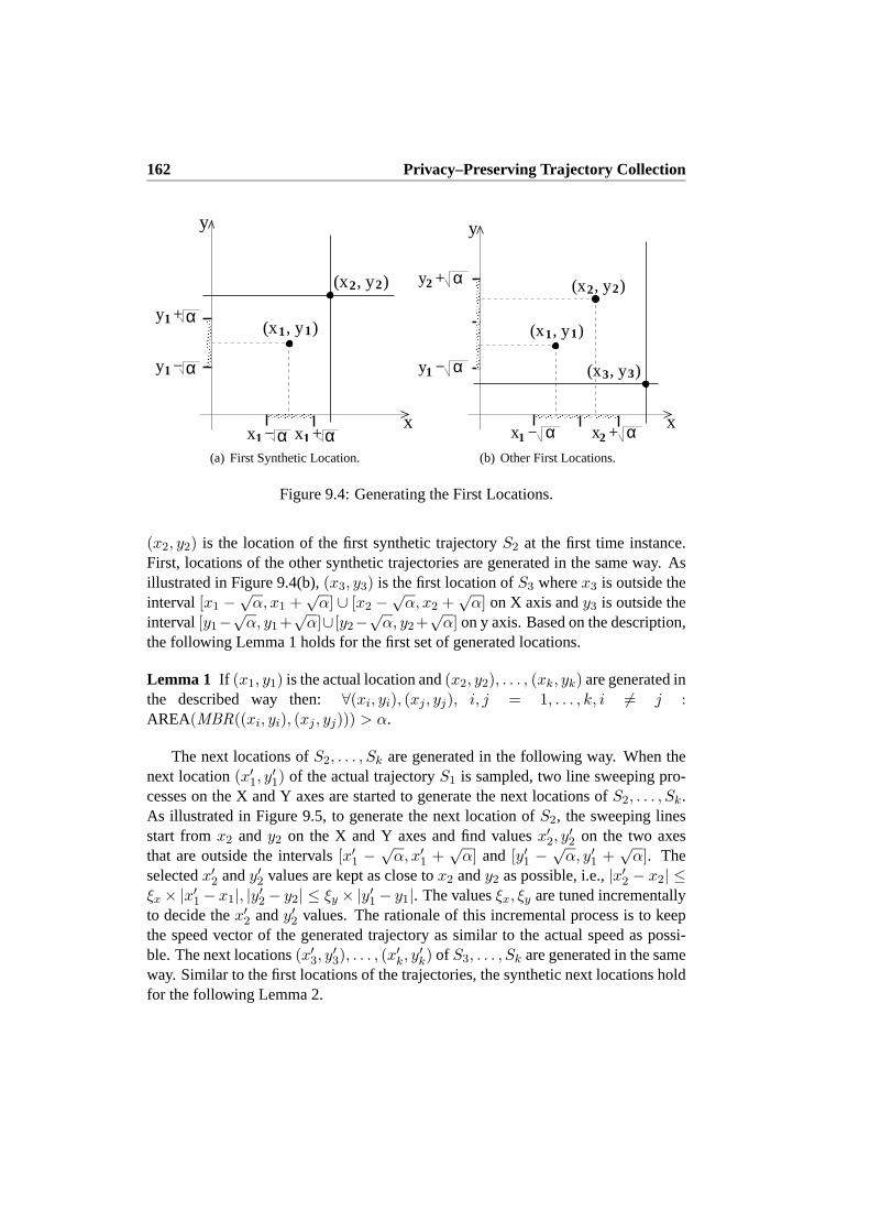
162 Privacy–Preserving Trajectory Collection
1 1
αx +1αx −1
αy −1
αy +1
(x , y )2 2
x
(x , y )
y
(a) First Synthetic Location.
1
(x , y )2 2
(x , y )3 3
2 αx +
αy −1
α1x −
αy +2
x
(x , y )
y
1
(b) Other First Locations.
Figure 9.4: Generating the First Locations.
(x2, y2) is the location of the first synthetic trajectoryS2 at the first time instance.First, locations of the other synthetic trajectories are generated in the same way. Asillustrated in Figure 9.4(b),(x3, y3) is the first location ofS3 wherex3 is outside theinterval [x1 −
√α, x1 +
√α] ∪ [x2 −
√α, x2 +
√α] on X axis andy3 is outside the
interval[y1−√
α, y1+√
α]∪ [y2−√
α, y2+√
α] on y axis. Based on the description,the following Lemma 1 holds for the first set of generated locations.
Lemma 1 If (x1, y1) is the actual location and(x2, y2), . . . , (xk, yk) are generated inthe described way then: ∀(xi, yi), (xj , yj), i, j = 1, . . . , k, i 6= j :AREA(MBR((xi, yi), (xj , yj))) > α.
The next locations ofS2, . . . , Sk are generated in the following way. When thenext location(x′
1, y′1) of the actual trajectoryS1 is sampled, two line sweeping pro-
cesses on the X and Y axes are started to generate the next locations ofS2, . . . , Sk.As illustrated in Figure 9.5, to generate the next location ofS2, the sweeping linesstart fromx2 andy2 on the X and Y axes and find valuesx′
2, y′2 on the two axes
that are outside the intervals[x′1 − √
α, x′1 +
√α] and [y′1 − √
α, y′1 +√
α]. Theselectedx′
2 andy′2 values are kept as close tox2 andy2 as possible, i.e.,|x′2 − x2| ≤
ξx × |x′1 − x1|, |y′2 − y2| ≤ ξy × |y′1 − y1|. The valuesξx, ξy are tuned incrementally
to decide thex′2 andy′2 values. The rationale of this incremental process is to keep
the speed vector of the generated trajectory as similar to the actual speed aspossi-ble. The next locations(x′
3, y′3), . . . , (x
′k, y
′k) of S3, . . . , Sk are generated in the same
way. Similar to the first locations of the trajectories, the synthetic next locationsholdfor the following Lemma 2.
9.4 Solution 163
1
(x , y )2 2(x’ , y’ )22
(x , y )3 3
(x , y )1 1
(x’ , y’ )33
y
(x’ , y’ )
x
1
Figure 9.5: Generating the Next Locations of Synthetic Trajectories.
Lemma 2 Assume the second locations(x′1, y
′1), . . . , (x
′k, y
′k) of each trajectory
S1, . . . , Sk where(x′1, y
′1) is the actual location and(x′
2, y′2), . . . , (x
′k, y
′k) are gen-
erated in the described way, then:∀(x′i, y
′i), (x
′j , y
′j), i, j = 1, . . . , k, i 6= j such that:
AREA(MBR((x′i, y
′i), (x
′j , y
′j))) > α.
Following the same way, subsequent locations of the synthetic trajectories are gen-erated. Based on Lemma 2, the area size of the MBR on every two locations oftrajectoriesS1, . . . , Sk at the same time instance is greater thanα. With Lemmas 1and 2, the area size of the MBR on all the trajectoriesS1, . . . , Sk is greater thanα.When the functionget pieceexecutes on the trajectoriesS1, . . . , Sk, the collectedtrajectories piecesS′
1, . . . , S′2 satisfy the following lemma.
Lemma 3 Assume the data items(id1, S′1), . . . , (idk, S
′k) are generated by function
get piece, then the area sizes for all of the MBRs of the trajectory piecesS′1, . . . , S
′k
is greater thanα and for any two trajectory piecesS′i, S
′j , i, j = 1, . . . , k, i 6= j, the
area size AREA(MBR(S′i, S
′j)) > α.
Based on Lemma 3, when the data items are added to the trajectory databaseDB, theMBR of all the trajectory pieces has an area size bigger thanα. Since there are atleastk data items in theDB and these data items havek different ID values, all thedata items atDB preservek–anonymityas well asα–diversitywhen a new group ofdata items are added toDB.
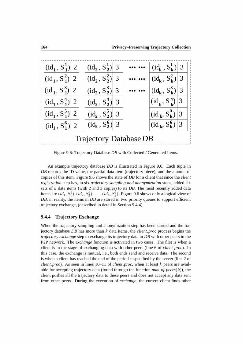
164 Privacy–Preserving Trajectory Collection
DB
2 2
2 24
2 23
2 22
2 21
(id , S ) 3
(id , S ) 3
(id , S ) 3
5
k k1
k k2
k k3
k k4
1 11
1 12
1 13
1 14
1 15
1 16
(id , S ) 2
262
k
k k
k5
(id , S ) 3
(id , S ) 26
(id , S ) 2
(id , S ) 2
(id , S ) 2
(id , S ) 2
(id , S ) 3
(id , S ) 3
(id , S ) 3
(id , S ) 3
(id , S ) 3
(id , S ) 3
(id , S ) 3
(id , S ) 3
... ...
... ...
... ...
Trajectory Database
Figure 9.6: Trajectory DatabaseDB with Collected / Generated Items.
An example trajectory databaseDB is illustrated in Figure 9.6. Each tuple inDB records the ID value, the partial data item (trajectory piece), and the amount ofcopies of this item. Figure 9.6 shows the state ofDB for a client that since theclientregistrationstep has, in sixtrajectory sampling and anonymizationsteps, added sixsets ofk data items (with 2 and 3 copies) to itsDB. The most recently added dataitems are(id1, S
61), (id2, S
62), . . . , (idk, S
6k). Figure 9.6 shows only a logical view of
DB, in reality, the items inDB are stored in two priority queues to support efficienttrajectory exchange, (described in detail in Section 9.4.4).
9.4.4 Trajectory Exchange
When the trajectory sampling and anonymization step has been started and the tra-jectory databaseDB has more thank data items, theclient proc process begins thetrajectory exchangestep to exchange its trajectory data inDB with other peers in theP2P network. Theexchangefunction is activated in two cases. The first is when aclient is in the stage of exchanging data with other peers (line 6 ofclient proc). Inthis case, the exchange is mutual, i.e., both ends send and receive data. The secondis when a client has reached the end of the periodτ specified by the server (line 2 ofclient proc). As seen in lines 10–11 ofclient proc, when at leastk peers are avail-able for accepting trajectory data (found through the functionnumof peers(k)), theclient pushes all the trajectory data to these peers and does not accept any data sentfrom other peers. During the execution ofexchange, the current client finds other

9.4 Solution 165
clients running the same function and exchanges the trajectory data from its databaseDB. The parameterstateof function exchangespecifies whether the current clientwants mutual data exchange (state = TRUE ) or to only push data to other peers(state = FALSE ). The pseudo code ofexchangeis listed bellow.
(1) procedureexchange(k,DB , state)(2) p1, . . . , pm ←find peers(k)(3) for eachpi, i = 1, . . . , m(4) DB in,DBout ← ∅(5) t ←get state(pi)(6) if t = TRUE
(7) DBout ←pick items(k,DB)(8) DB←DB\DBout
(9) send(pi,DBout)(10) if state = TRUE
(11) get(pi,DB in) // DB in : di′1, . . . , di′ki
(12) else:get(pi,DB in)(13) DB← DB ∪ DB in
(14) return
The algorithm first searches for peers from the P2P network (line 2). Then, theclient starts a while–loop to communicate with each of the peers (lines 3–14). Whena peerpi is connected, the algorithm first readspi’s state (line 5), i.e., whetherpi
wants mutual exchange or only wants to push its data to other peers. Ifpi wantsmutual exchange, the current client selectsk items fromDB, puts the items into a setDBout, and uses functionsend to send the data to peerpi (lines 7–9). If the currentclient wants mutual exchange, the functionget is called to accept data frompi (sentby thesend function atpi) to a local setDB in (lines 10–12). Ifpi only wants topush its data to the current client, the functionget is also called to accept the data toDB in (line 13). Finally, the data items inDBout are removed fromDB (line 8) andthe fresh items frompi are read intoDB (line 14).
The functionfind peers(k) finds nearby mobile clients in the P2P network thathave at leastk clients in their respective vicinities. To protect a client from sendingtoo much data to a single and perhaps malicious peer, the function uses a small FIFObuffer that keeps a list of the recently–contacted peers and avoids sending too muchdata to these peers.
The functionpick items is used for pickingk partial data items from the tra-jectory database. It works as follows. First, it picks two collected/generated items.Then, it picksk − 2 items that were received in previous exchanges. To ensure thatthere are always at least two collected/generated items to pick from, when thenumberof such items is very small, extra copies of them are generated without alteringthe

166 Privacy–Preserving Trajectory Collection
DB
2 2
2 24
2 23
2 22
2 21
(id , S ) 35
k k1
k k2
k k3
k k4
1 11
1 12
13
1 14
1 15
1 16
262
k
k k
k5
(id , S ) 3
(id , S ) 26
(id , S ) 2
(id , S ) 2
(id , S ) 3
(id , S ) 3
(id , S ) 3
(id , S ) 3
(id , S ) 3
... ...(id , S ) 0
(id , S ) 0
(id , S ) 1 (id , S ) 0
(id , S ) 3
k+2’
(id , S ) 0 k+1’
k+3’
k+4’
k+m’
k+4’4
k+m’6
k+3’3k+2’3k+1’1
... ...(id , S ) 1
(id , S ) 1
(id , S ) 1
(id , S ) 1
(id , S ) 0
Data Itemsfrom PreviousExchanges
... ...
... ...(id , S ) 21
(id , S ) 1
22Items Ready for Exchange2(id , S ) k k
3(id , S ) (id , S )k+1’ k+1’1 (id , S )k+2’ k+2’
3
Maximal Anonymity Set
Trajectory Database
Figure 9.7: State ofDB After Several Exchanges.
parities, i.e., always an even number of extra copies are generated. If there are notenough previously exchanged items to pick from, the function picks the remainingitems from the collected/generated items. All of the items are picked in order of ageand number of copies, i.e. the oldest item with the most number of copies first; tiesare broken at random. All of the picked items have different ID values. When anitem is picked, the corresponding copy amount of the item is reduced in the trajec-tory databaseDB. For each item inDB, if the copy amount is reduced to 0, the itemis erased fromDB.
A concrete example of the item selection is shown in Figure 9.7. Since the sixinitial trajectory sampling and anonymizationsteps, the client has performed severalexchange steps in which it receivedm data items with IDsidk+1′ , . . . , idk+m′ , andsent all copies of some of its collected/generated items, f.ex.,(id1, S
11), shown in
shaded cells. According to “the oldest with the most copies” selection criteria, thepick items function picks two collected/generated items(id2, S
22), (idk, S
3k) and two
previously exchanged items(idk+1′ , S1k+1′), (idk+2′ , S
3k+2′) for exchange. The copy
amounts of the selected items are only updated after the items have been successfullyexchanged.
The above selection can be easily accommodated by storing the collected/generat-ed and previously exchanged items in two priority queuesPQcg andPQex , respec-tively. Items are prioritized according to their age and copy amount (oldestwith mostcopies first) in their respective queues. The queues support the following four oper-

9.4 Solution 167
ations: insert, delete, increase/decreasethe priority of an element, andpeekat thetop k elements. Using a Fibonacci heap implementation, most of the operation canbe supported in amortized constant time (deletions are still O(log n)) [16]. Using thequeue operations, thepick items function can be implemented as follows.Peekatthe top 2 elements ofPQcg , and the topk − 2 elements ofPQex ; consider the itemsin these elements for exchange. After a successful exchange of the items, dependingon the copy amount of the exchanged items prior to the exchange, eitherdecreasethepriority of an element based on the updated copy amount, ordeletethe item from thequeue if the last copy has been exchanged.
A number of aspects of the selection process performed by thepick items func-tion is important to emphasize. First, the items picked by thepick items functionhavek different ID values and the MBR of at least two items has an area size largerthanα. Hence, the items picked for exchange satisfyk–α–anonymity.Second, theselected collected/generated items are the oldest amongst all such items and corre-spond to trajectory pieces from the past. Hence, the trajectory pieces described bythese items are spatially disconnected from the location where the exchange istakingplace, which prevents a malicious client from making inferences based on such a con-nection. Third, the selection process ensures that the oldest items are exchanged firstand that the distribution of the number of remaining items for different IDs is ascloseto uniform as possible. These latter aspects are important for reaching / maintaininganonymity state, which is defined next.
When theexchangeprocess has been started for a while, and the client has re-ceived data items form ≫ k ID values from other clients, identification of the actualtrajectory of the client becomes less trivial. Nonetheless, if the entireDB was re-ported to the server, the server, based on the number of data items for each ID, couldwith high probability associate a set ofk IDs with the client. Later, during thedatasummarizationstage, the server could identify the actual trajectory of the client by fil-tering out synthetic trajectories. To study when a part ofDB is k–anonymoustowardsthe server, theanonymity stateof a subset of data items is defined as follows.
Definition 12 (Anonymity state) A given subsetS of the data at a clientc is inanonymity stateif there are at leastk − 1 IDs from other clients and the distribu-tion of the number of partial data items for the different IDs is statistically equaltothe uniform distribution according to the Kolmogorov–Smirnov One–Sample testfora given critical valueαKS
1.
1The Kolmogorov–Smirnov One–Sample (KS–1) test is a goodness–of–fit test between an empiricaldistributione and a known distributionu [71]. According to the KS–1 test the null hypothesis,e notbeing significantly different fromu, can be rejected at a confidence levelp = 0.05 if the maximumabsolute difference between the cumulative distribution ofe andu is larger than a critical valueαKS =
1.36/√
n for a sample size ofn > 35.

168 Privacy–Preserving Trajectory Collection
The subsetS in practice contains collected/generated items ranging from the oldestuntil the most recent collected/generated item that can be included while still main-taining anonymity state. The exchanged items in the subsetS span a time period thatincludes the time period that is spanned by the collected/generated items in the sub-set. The largest possible subset of the data in anonymity state is called themaximalanonymity set. In Figure 9.7, items in cells with think borders comprise the maximalanonymity set .
Given the way items are picked for exchange, the way FIFO buffers areem-ployed at each client to avoid sending data too many times to the same client, andthe likelihood of re–encountering the same client, the likelihood of receiving severaldata items for the same ID is very low. Hence, for practical purposes, the entiretrajectory databaseDB of client c is in anonymity state if it contains at leastk − 1items from other clients, and it contains on average at most one data item for eachof c’s IDs. To achieve anonymity state, a client has to exchange most of its col-lected/generated data items. There areni ∈ 2z, 2z + 1 : z ∈ Z
+ copies ofk dataitems collected/generated per sampling (λ) period. Since in one exchange process,with the exception of the initial conditions, two of these items are selected for ex-change,⌈k × ni/2⌉ exchanges are necessary to send all of the client’s own data topeers. Assume that the client’s entireDB was in anonymity state at timeta, and nodata exchange occurred up to timetnow = ta+n∗λ. Then, the client needs to partici-pate in at least⌈n×k×ni/2⌉ exchanges during the period[ta+n×λ, ta+(n+1)×λ)for its entireDB to be in anonymity state again. Assuming the number of possibleexchanges a client can perform is uniform over time, a client is said tomaintainanonymity state if it participates, on average, in at least⌈k × ni/2⌉ exchanges persampling period. In a concrete example, if the client collects/generates 2 and3 copiesof k = 5 items per sampling period, the client maintains anonymity state if it partici-pates, on average, in at least⌈5 × 3/2⌉ = 8 exchanges per sampling period.
Based on the above discussion, anonymity state may not be achieved if the clientdoes not have a good amount of data exchange with peers. The empiricalstudy inSection 9.6 investigates under what conditions and privacy settings the amount ofdata exchanges performed by clients is sufficient for clients to reach andmaintainanonymity state.
9.4.5 Data Reporting
Thedata reportingstep is activated in two cases. First, when theclient proc processis in the periodτ , and the size of the trajectory databaseDB is close to the storagelimit or the DB has partial data items that are too old (line 8 ofclient proc). Second,when a client has reached the end of the periodτ , in which case the client can eithersend out its data via exchange processes to other peers in the P2P network or continuewith thedata reportingstep.
9.4 Solution 169
The report function is started at thedata reportingstep. If thereport functionis invoked in the first case, it sends all of the data items obtained from other peersto the server and keeps the other data items. If thereport function is invoked in thesecond case, it sends the maximal anonymity set to the server and erases rest of the(collected/generated) data items at the client.
By erasing some of the most recently collected/generated data items, the recentpieces of a trajectory are lost. To reduce the extent of this loss before it occurs, theclient can dynamically, depending on the current time and the end of the period τ , inthetrajectory exchangestep increase the number of collected/generated data items inthe set ofk items that are selected for exchange. The empirical evaluations in Sec-tion 9.6 show that, even without clients performing the above outlined loss reductionstrategy, the loss is negligible. Ultimately, the loss can also be entirely eliminated,if the client at the end of the periodτ saves the remaining collected/generated itemsand restarts theclient proc at theclients registrationstage. Since the saved itemsare the oldest items amongst the newly collected/generated data items, they will beselected first by thepick items function in future exchanges. Hence, the probabilitythat the client re–reports items for one or more of its previous IDs in the nextdatareporting stage, thereby sacrificing its privacy towards the server, isvery low. Tocompletely eliminate the above probability the client can optionally flag the saveditems and ensure that no flagged items are reported to the server. This flagging tech-nique effectively trades a slim probability for the loss of privacy againsta negligibleloss in the trajectory.
In the very unlikely event when a clientc is not able to perform a single ex-change within theτ period, and hence has an empty maximal anonymity set, theentire trajectory of a client is erased and not reported to the server. Even in this casethek–anonymityof the otherk − 1 clients started at the same time asc will not bechanged. Specifically, if there is only one client that reports data and the otherk − 1clients erase their collected/generated data, the server still does not knowwho thistrajectory refers to among thek clients.
9.4.6 Data Summarization
Thedata summarizationstep starts theserversumprocess. This process keeps run-ning to collect data from clients and summarizes the data into trajectories. Specif-ically, when the server receives data from clients, theserversumprocess maintainsa temporary tablethat arranges the received partial data items into groups based onthe ID values of the items. As illustrated in Figure 9.8, thetemporary tableputs allpartial data items with the same ID values under the same row .
Theserversumprocess also records the timestamps when the first data item ofeach column is received (t1, t2, t3, . . . in Figure 9.8. These timestamps are used todetermine when the items under each ID value have been fully received. Specifically,

170 Privacy–Preserving Trajectory Collection
2
id : 15S
12id :
45S
212S1
12S 312S 4
12S
35S2
5S
Summary Table Temporary Table
Process at the Server Sideserver_sum Client Data...... ...
2
...
...
...... ... ... ...
S S Sid :1 11
12
1S314 1
11
t 3
t 2
t 1
21
2
11
5
333
1 13
2
3
5 52
62
33
4
5
7
9
5
7
93
7
6
6
(id ,S )
(id ,S )
(id ,S )
(id ,S )
(id ,S )
(id ,S )
3 3
51
1(id ,S )
(id ,S )
(id ,S )
(id ,S )
(id ,S )
(id ,S )(id ,S )
2
32
5
Figure 9.8: Data Summarization.
suppose the first data item of a column in the summarization table is received at timet1. Then theserversumprocesses waits for a2τmax time period to wait for the restof the data items of the same ID value to be sent from the clients. Since data itemsolder thanτmax at every client are required to be sent to the server, all the data itemsof the column should have been received after a2τmax time period sincet1. Afterthis period, theserversumprocess checks the amounts of copies of the data items ineach group. If the parities of the amounts in a group are odd, the group is removed asit represents cloaking data items. If the parities in the group are even, the trajectorypieces in this group are merged into a whole trajectory based on the timestamps ofthe trajectory pieces. Finally, as illustrated in Figure 9.8, the actual trajectories arerecorded in asummary tableand saved at the server database.
It is possible that not all copies of a data item are reported to the server. Forexample the missing copies could be part of the loss described in Section 9.4.5.Thecopies could also be missing because a malicious client deliberately deleted or alteredthe copies. In these cases, checking the parity of the amount of copies ofa single dataitem alone would be misleading. Hence, instead of performing parity checks of copyamounts of individual data items, a check for the majority parity of copy amountswithin a group is performed.

9.5 Discussion 171
9.4.7 Neighborhood Detection in P2P Networks
The functionfind peers(k), on line 2 of theexchangefunction, finds nearby mobileclients in the P2P network that have at leastk clients in their respective vicinities. Itis executed in order to ensure that exchanges satisfy the second condition of thek–anonymitydefinition (Definition 9). In a trusted P2P environment, where clients canbe trusted, thefind peers(k)–query can be answered in a straight forward fashion, i.e.,the client asks its neighbors about their neighbors and decides based onthe answers.In an untrusted P2P environment, where potentially malicious clients might try to lieabout their neighbors, answers from individual peers can still be verified based onthe totality of the answers as follows. First, the acquiring clientci asks its neighborsCn = cl, . . . , cm for their neighbors’ IDsIn = Il, . . . , Im. Then, clientci
summarizes the ID sets,In, and retains the IDs,Iv, that are present in more thanmin verif cnt number of ID sets. Assuming that there are at mostmin verif cnt −1 malicious andcooperatingclients among the clientsCn, theverifiable IDs of anID setIj ∈ In areIj ∩ Iv. Consequently, a clientcj ∈ Cn is part of the answer setto theverified findpeers(k)–query if |Ij ∩ Iv| ≥ k. Naturally, if there is very littleoverlap between thetrue ID sets, i.e., the size ofIv is very small, then this verificationmethod will reject answers from non–malicious clients and thereby limit the numberof possible exchanges. However, the fraction of thetrue answers that are rejected bythe proposed verification method turns out to be very small in practice, as is shownby the experiments in Section 9.6.
9.5 Discussion
The proposed solution aims to collect trajectory data while keeping each mobileuser’s trajectory anonymous among other trajectories. The anonymity settings arekept in the privacy profile of each client. Due to the big variety of privacythreats, thepossible privacy risks are generalized into three categories: privacyrisk at the serverside, the client side, and in the air. In the following each of these risks is discussed.
9.5.1 Privacy at the Server
In the server side application, in accordance with each set ofkmax mobile users(kmax is the maximalk value sent by all these users) that start data collection atthe same time, there will be the same or less amount of trajectories returned by thedata summarizationstep. Since the ID values are generated at the client side, it isimpossible to link a moving object with a specific trajectory. Thus, the requirementof k–anonymityof the clients is preserved at the server side.

172 Privacy–Preserving Trajectory Collection
9.5.2 Privacy at Clients
Each client, after starting thetrajectory sampling and anonymizationand thetrajec-tory exchangesteps, has at leastk (k is defined by its own privacy profile) groups ofdata items with different ID values. After a client has achievedanonymity state, thedata items at this client satisfyk–anonymity. Based on Lemma 3, the area size of theMBR of all the data items inDB can always be kept overα. Thus, the data items atthe client also satisfyα–diversity.
9.5.3 Privacy in the Air
Data is transmitted in the air in two cases. The first is when the data is exchangedbetween peers in the P2P network. As described in thetrajectory exchangestep,each client sendsk data items with different ID values and the area size is kept overα. Thus, the data transmitted between peers preservesk–α–anonymity. The secondcase happens when a client reports the data to the server. Based on the description ofSection 9.4.5, this client sends either only the exchanged data from other peers or themaximal anonymity set to the server. Thus, the data in the air satisfiesk–anonymityandα–diversityin this case.
The proposed solution for trajectory collection preserves thek–anonymityin all as-pects of the data collection process. The solution does not change the actual trajec-tory data, but usescloaking data itemsto preserve the anonymity, the accuracy of theoriginal data is guaranteed. Since the server can have more safety protections such asfirewalls and many other softwares to safeguard the data, the clients and thedata be-ing transmitted are more fragile under various forms of privacy threats. The proposedsolution have further anonymity protection, such asα–diversityandk–α–anonymity,at the clients and the data in the air. To summarize, the proposed solution preservesthe accuracy of the collected data and achieves anonymity requirements by taking theadvantage of the P2P network to swap and anonymize the data at the clients.
9.6 Empirical Evaluation
The effectiveness of the proposed privacy preserving trajectory collection methodwas empirically evaluated for a simulated shopping mall environment. A grid–basedshopping movement simulator was developed to generate realistic movements ofclients in a 177,200m2 large shopping mall with 16 shops. In the simulation, clientsmove from a 5×5–meter grid cell to a neighboring grid cell at a speed of 1 m/sec. Asimulation step is 5 seconds long, i.e., a client can only move at most one grid cellinone simulation step. The movements of clients are random, but obey the followingrules:

9.6 Empirical Evaluation 173
Figure 9.9: Layout of the Shopping Mall with a Sample Shopping Trajectory.
1. A client never crosses a wall.2. A client at each step picks a random direction obeying rule 1) and preferring
a direction that was the same as its previous direction of movement. Thispreference is defined by aheading factor parameter which for higher valuesmakes clients move more in a straight line. This parameter is different for thecorridor environment and the shop environment, in order to simulate transitionlike movement between shops and browsing like movement within shops.
3. A client never visits a shop twice.4. A client becomes idle with probabilitybrowsing prob inside shops, this essen-
tially slows down the average speed of the client inside a shop.5. A client, obeying rule 3), is drawn with a certain strength into a shop as it
passes the door of the shop, the strength of this drawing force is controlled bya parameterentrance factor .
The layout of the shopping mall used in the simulations and a two hour longsample trajectory of a simulated client is shown in Figure 9.9. In the example shownand in all of the simulations theheadingf actor was twice as large in the corridorenvironment than in the shop environment, and thebrowsingprob parameter was setto 0.25, resulting in an average speed during browsing that is1/4 of the normalwalking speed.
The effectiveness of the proposed method was evaluated using four measures: 1)the fraction of clients that reached anonymity state at some point during the simula-tion period, 2) the fraction of collected/generated data items that are held by clientsresponsible for collection/generating them, 3) the number of exchanges performed
174 Privacy–Preserving Trajectory Collection
by clients per sampling (λ) period, and 4) the ages of the oldest collected/generateddata items that are held by clients responsible for collection/generating them. Threegroups of 20–minute long simulations were performed varying the number of clientsm, the anonymity parameterk, and the communication ranger in the P2P network.The sampling period in all of the experiments was fixed atλ = 60 seconds, duringwhich each client collected/generatedn ∈ 2, 3 copies ofk data items. Duringan exchange a client, if possible, sent2 of its oldest collected/generated data itemsandk − 2 of its previously received data items. In all the experiments, each client’sFIFO buffer for recording recently–contacted peers was 10 elements long. The re-sults of the three groups of experiments are shown in Figures 9.10, 9.11, and 9.12,respectively.
Figures 9.10(a)–9.10(c) show the four effectiveness measures foranonymity pa-rameterk = 5 and communication ranger = 10 meters, for varying number ofclients. As the number of clients increases, i.e., the spatial density of clients in-creases, the average number of exchanges an average client can perform during asampling (λ) period also increases, see Figure 9.10(b). Given the particular settingsfor k andn, the average number of exchanges a client needs to perform per samplingperiod to reach (maintain) anonymity state is about 7.5 (5), which is achieved bymost clients in the case of 2,000 clients. Under these conditions, most of the clientssuccessfully have managed to exchange most of their old collected/generated dataitems and only hold own data items that have been collected/generated in the last fewsampling periods, see Figure 9.10(c). The same results, viewed at a system level, areshown in Figure 9.10(a), where it can be seen that as the number of clients, i.e., thespatial density of the clients increases, the fraction of clients that reach, and with asufficiently high likelihood, maintain anonymity state during the simulation periodalso increases. Similarly, due to the increasing number of exchanges, an increasingfraction of the total amount of colected/generated data items have been passed ontoother clients and consequently a decreasing fraction of the data items is present in thesystem in a less anonymized state, held by the producing client.
Figures 9.11(a)–9.11(c) show the four effectiveness measures foranonymity pa-rameterk = 5 andm = 1, 000 clients for varying communication ranger. Theresults are similar to the previous results. That is, as the communication range isincreased, the number of exchanges increases (Figure 9.11(b)), theages of the oldestdata items held by the producing clients decreases (Figure 9.11(c)), the fraction of theclients that reach (maintain) anonymity state increases, and the fraction of thetotaldata items that is in a less anonymized state decreases (Figure 9.11(a)). It isimportantto note that the effects of the communication range parameter are more pronounceddue to the quadratic relationship between the communication range and the numberof exchanges (Figure 9.11(b)).

9.6 Empirical Evaluation 175
250 500 750 1000 1250 1500 1750 20000
0.2
0.4
0.6
0.8
1
number of clients
fraction of data items that are held by clientsfraction of clients that reached anonymity state
(a) Anonymity State and Data Dissemination.
250 500 750 1000 1250 1500 1750 20000
2
4
6
8
10
12
number of clients
avg
# of
exc
hang
es /
λ p
erio
d medianmean with std errorminimummaximum
(b) Number of Exchanges per Sampling Period.
250 500 750 1000 1250 1500 1750 20000
5
10
15
20
number of clients
age
of th
e ol
dest
dat
a ite
m (
in λ
per
iods
)
medianmean with std errorminimummaximum
(c) Age of Oldest Data Item.
Figure 9.10: Efficiency Evaluation for Varying Number of Clients.
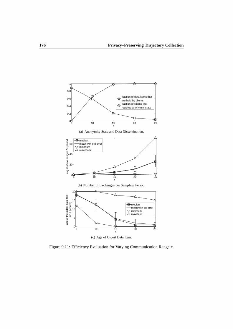
176 Privacy–Preserving Trajectory Collection
5 10 15 20 250
0.2
0.4
0.6
0.8
1
r
fraction of data items that are held by clientsfraction of clients that reached anonymity state
(a) Anonymity State and Data Dissemination.
5 10 15 20 250
20
40
60
r
avg
# of
exc
hang
es /
λ p
erio
d medianmean with std errorminimummaximum
(b) Number of Exchanges per Sampling Period.
5 10 15 20 250
5
10
15
20
r
age
of th
e ol
dest
dat
a ite
m
(inλ p
erio
ds)
medianmean with std errorminimummaximum
(c) Age of Oldest Data Item.
Figure 9.11: Efficiency Evaluation for Varying Communication Ranger.

9.6 Empirical Evaluation 177
3 4 5 6 7 8 9 100
0.2
0.4
0.6
0.8
1
k
fraction of data items that are held by clientsfraction of clients that reached anonymity state
(a) Anonymity State and Data Dissemination.
3 4 5 6 7 8 9 100
5
10
15
k
avg
# of
exc
hang
es /
λ p
erio
d medianmean with std errorminimummaximum
(b) Number of Exchanges per Sampling Period.
3 4 5 6 7 8 9 100
5
10
15
20
k
age
of th
e ol
dest
dat
a ite
m
(inλ p
erio
ds)
medianmean with std errorminimummaximum
(c) Age of Oldest Data Item.
Figure 9.12: Efficiency Evaluation for Varyingk–Anonymity.
Figures 9.12(a)–9.12(c) show the four effectiveness measures forcommunicationranger = 5 meters andm = 2, 000 clients for varying anonymity parameter valuesr. Increasing values for anonymity parameter valuek results in decreasing numberof possibilities for exchange and increasing amount of colected/generated data itemsto be exchanged. Hence the total effect of these changes affect the effectivenessmeasures in an inverse manner to the effects of the parametersm andr.

178 Privacy–Preserving Trajectory Collection
2 3 4 5 6 7 8 9 100.4
0.5
0.6
0.7
0.8
0.9
1
k
true
/ ve
rifia
ble
find_
peer
s(k)
min_verif_cnt = 2min_verif_cnt = 3min_verif_cnt = 4min_verif_cnt = 5min_verif_cnt = 6min_verif_cnt = 7min_verif_cnt = 8min_verif_cnt = 9min_verif_cnt = 10
Figure 9.13: Fraction offind peers(k) Answers that are Verifiable for Varying Valuesof k andmin verif cnt .
In all of the so far presented experimental results, thefind peers(k)–queries wereexecuted assuming that there are no malicious clients. As proposed in Section9.4.7,with a rather simple method the answers to thefind peers(k)–queries can easilybe verified by the clients even in case of multiple and potentially cooperating ma-licious clients. To determine the effectiveness of the proposed verificationmethod,500 uniform random points were generated in the unit square, representing locationsof clients, and the true versus verifiable answer sets tofind peers(k)–queries havebeen compared for all the points for varyingk andmin verif cnt parameters and afixed communication range ofr = 0.1. To eliminate the effects of randomness, themeasurements are based on 100 independent test runs. The results of these exper-iments are shown in Figure 9.13. The trends in the results are as expected, i.e., asthe values of thek andmin verif cnt parameters increase the fraction of answersthat are verifiable using the proposed method decreases. However, it isinteresting tosee that for rather high values ofk andmin verif cnt the fraction is relatively high.In particular, assuming there is at most one malicious client near the client issuingthefind peers(k)–query, the client can verify over 90% of the answers even in thecase of largek parameter values. Consequently, using the proposed verification me-thod, even in an untrusted environment clients can perform most of the exchangesand hence reach and maintain anonymity state.
In summary, the experimental results show that the proposed privacy preservingtrajectory collection method is effective, i.e., under reasonable conditions (m, r) andfor anonymity parameter values (k), clients are able to perform exchanges frequentlyenough, so that within a short period of time (1 - 5 minutes) most clients are in

9.7 Conclusions and Future Work 179
anonymity state and only a small fraction of the data items is in a less anonymizedstate, held by the producing client.
9.7 Conclusions and Future Work
The paper considered the problem of collecting trajectories of moving objects in aprivacy–preserving manner. As a premiss for studying the problem, the paper firstadapted and combined previously proposed general data privacy definitions to derivedefinitions for location privacy. The derived location privacy definitions in increas-ing strength are:k–anonymity, α–diversity(requiring spatial diversity), andk–α–anonymityof location data. To solve the problem, the paper proposed a completesystem for thelossless, privacy–preserving collection ofexacttrajectories of movingobjects. The proposed system is based on a client–server architecture and the collec-tion process can be summarized into five stages, namely: 1)client registration, 2) tra-jectory sampling and anonymization, 3) trajectory exchange, 4) data reporting, and5) data summarization. The proposed system does not require trusted components,yet it guarantees at leastk–anonymityin all stages of the collection process. Theproposed system isscalableas the process of anonymization is performed in a dis-tributed fashion by clients interacting via an assumed wireless P2P network. Finally,through an extensive empirical evaluation, the paper demonstrated that theproposedsystem is effective under reasonable conditions and privacy/anonymitysettings.
Future work will be along four paths. First, different kinds of system architec-tures will be considered. For example, as is common in wireless P2P network re-search [100], the addition of hotspots to the P2P network will be considered. Thesehotspots will further reduce the chance of isolated clients and could potentially beused to distribute theclient registrationanddata summarizationstages. Second, fu-ture work will consider the implementation of a full system and the large–scale real–world deployment of the system. Third, satisfying thek–anonymityof exchangeseven in the presence of malicious clients is essential to the proposed system. Initialexperiments indicate that the proposed method to verifyfind peers(k)–query resultsin a P2P network is effective. Nonetheless, it is only one possible solution toan-swer the query in a P2P network with malicious clients. Future work will considerother methods that guarantee even higher accuracy or security. Finally,a theoreticalline of work will consider 1) proving the robustness of the system, and 2) finding atheoretical model of the system performance in relation to privacy protection.


Chapter 10
Summary
Several hardware trends in mobile technology, in particular the increasingavailabilityand accuracy of mobile position technologies, pave the road for LBSes. InnovativeLBSes integrate knowledge about the mobile user into the service. Much knowledgecan be gained about users by analyzing the location data of users. To thisextent,this thesis 1) devised effective spatio–temporal data mining methods for the desiredanalysis, 2) demonstrated the usefulness of the spatio–temporal data mining methodsin promising LBS examples, and 3) devised privacy–preserving systems for trajectorycollection and analysis.
10.1 Summary of Conclusions
The conclusions from Chapters 2 to 9 are the following. Chapter 2 proposed pivotingas a general methodology to extend a popular data mining method, namely rule min-ing. By considering a number of different types of data sources, the chapter deriveda taxonomy of spatio–temporal data and investigated the types of knowledge that canbe extracted using the extended spatio–temporal rule mining method.
Chapter 4 used pivoting to extend a frequent itemset mining method to find longsharable routes in trajectories. Considering different modelling options for trajec-tories led to the development of two variants of the method that can analyze largeamounts of trajectories. High–level SQL–based implementations are described, andextensive experiments on both real–life- and large–scale synthetic data show the ef-fectiveness of the method and its variants. The knowledge that the method and itsvariants can discover are believed to be useful for traffic planning andoptimizationand LBSes in the transportation domain.
Since real–world data sets about large populations of moving objects are difficultto obtain, to aid the development in spatio–temporal data management and analysis,Chapter 3 developed ST–ACTS, a Spatio–Temporal ACTivity Simulator. By using a
181
182 Summary
number of real–world data sources and intuitive principles, ST–ACTS models someof the so far neglected social and geo–demographical aspects of mobility.Experi-mental results showed that ST–ACTS is able to effectively generate realisticspatio–temporal activities of a large population.
Some LBSes only make sense or are most effective if spatio–temporally closebyservice requests are served in a group. Chapter 5 presented one example of such anLBS, namely a cab–sharing service. To provide an effective service the chapter pro-posed an algorithm for grouping closeby cab requests into a cab–shareto minimizethe total transportation cost, or equivalently maximize the savings. The algorithmwas expressed as a sequence of simple SQL statements. Experiments basedon sim-ulated request data demonstrated that the proposed algorithm can effectively grouptogether requests and thereby achieve significant savings.
In Chapter 6, the grouping algorithm was suggested as a generic building blockto optimize large–scale collective transportation systems. To scale the algorithmto alarge request stream, it was expressed as a continuous query in a Data Stream Man-agement System (DSMS), the problem was sub–divided through static andadaptivespatial stream partitioning methods, and the computation was parallelized using thepartitioning methods and the facilities of the DSMS. Experimental results showedthat using the adaptive partitioning methods, the parallel implementations executeseveral orders of magnitude faster, yet achieve almost the same quality ofgroupingas their serial equivalent.
Location–Based Advertising (LBA), i.e., deliveringrelevantcommercial infor-mation to mobile consumers, is regarded by many as one of the most lucrative busi-ness opportunities in LBSes. In order to give an indicator for the magnitudeof thisopportunity, in Chapter 7 an LBA framework and database was developedand usedto estimate the capacity of the LBA channel. The proposed framework modelsrele-vanceas a function of theproximityof the consumer to the service/product and theinterestof the consumer. Two interest cases were considered:explicit and implicit.The chapter outlined several data mining techniques to infer the latter implicit inter-est. Experimental results showed that the channel capacity is indeed extremely large,which not only supports a business case, but also indicates the necessityof adequateuser controls.
Whenever data about users is collected and analyzed, privacy naturally becomesa concern. To eliminate this concern, Chapter 8 proposed a grid–based framework toanonymize, collect, and analyze location data. Since the proposed anonymization isthrough spatio–temporal generalization, i.e., the locations of users can be narroweddown to sub–regions with a certain probability only, the analysis results are alsoprobabilistic. To demonstrate the analysis component of the framework, the coredata mining task offinding dense spatio–temporal regionswas implemented. Experi-mental evaluations compared the results of the privacy–preserving mining method to
10.2 Summary of Research Directions 183
its non–privacy–preserving equivalent, and found that the privacy–preserving miningmethod can find most of the patterns.
To entirely eliminate the uncertainty in the mining results, Chapter 9 presenteda system for the privacy–preserving collection ofexacttrajectories. The system iscomposed of an untrusted server and clients communication via a P2P network. Lo-cation data is anonymized by the clients through data cloaking and data swappingtechniques. Experimental results based on simulated movements of mobile usersdemonstrated that the proposed system is effective under reasonable conditions andanonymity/privacy settings.
In summary, Chapters 2 through 9 demonstrated that common data mining meth-ods can be effectively extended to the spatio–temporal domain. The usefulness of theknowledge that the extended data mining methods can extract was demonstrated intwo promising LBSes: cab/ride–sharing service and location–based advertising. Fi-nally, to eliminate privacy concerns, systems were proposed for the privacy–preservingcollection and analysis of location data. Thus, the thesis has shown that commondata mining methods can be effectively extended to the spatio–temporal domain todiscover useful knowledge for LBSes in a privacy–preserving manner.
10.2 Summary of Research Directions
Several directions for future work remain. As Chapter 2 demonstrated, pivoting is ageneral methodology that can extend rule mining methods to discover usefulspatio–temporal rules. Spatio–temporally restricted rule mining was proposed to speed upthe mining process by processing meaningful spatio–temporal subregionsin isola-tion. Devising an automatic or semi–automatic system to determine these subregionsis believed to be an interesting research direction.
As Chapter 4 demonstrated, spatio–temporal generalization is an effectiveme-thod to discretize the spatio–temporal domain. Frequent itemset mining methods caneffectively discover patterns in sets of generalized spatio–temporal items.Such amethodology however does have some shortcomings. First, closeby locationmea-surements may fall in neighboring, butdifferentspatio–temporal regions. This re-duces the support of some patterns and potentially eliminate their discovery. Assuggested in Chapter 4, road network based spatio–temporal generalizations is oneapproach to overcome this problem. In situations where the movements of objects isnot confined to a road network, future work could consider the multi–grid approach,outlined in Chapter 8, as a way of reducing or eliminating the pattern support loss.Second, frequent itemset mining methods treat two spatio–temporally generalizeditems irrespective of their spatio–temporal proximity. As a consequence, mining re-sults will likely contain several spatio–temporally very similar patterns, which couldbe represented by a single pattern. While post–analysis can aggregate thesimilar pat-

184 Summary
terns, it is not an optimal approach as considering spatio–temporal item–proximityduring the mining can speed up the mining process and eliminate some of the pat-tern support loss. Hence, devising effective frequent itemset mining methods thatconsider spatio–temporal item–proximity is believed to be an interesting future re-search direction. Mining based on dimensional hierarchies could be helpful to deter-mine spatio–temporal item–proximity. The hybrid method to discover long, sharableroutes in trajectories was demonstrated to be an effective trajectory analysis tool.However, as it was demonstrated on simple examples, due to the hybrid modellingof trajectories the method might not discover all patterns, or due to the approximatedtrajectories might discover false patterns. Evaluating the accuracy of the hybrid me-thod is considered to be a valuable extension to the results of Chapter 4.
The simulator in Chapter 3 models only some of the physical aspects of mobil-ity. Integrating the output of ST–ACTS as an input to a sophisticated network–basedmoving object simulator is believed to yield synthetic data sets that could aid the de-velopment in telematics, intelligent transportation systems, and location–based ser-vices. Furthermore, the modelling capabilities of ST–ACTS can be extended togen-erate even more realistic activities of users. Some possible extensions are as follows.First, given the available real–world data sets, ST–ACTS models activities in terms ofdaily activity probabilities and spatio–temporal activity constraints. While this mod-elling approach allows ST–ACTS to generate data with spatio–temporal activitydis-tributions that correspond to the probabilities and obey the constraints, the generatedactivity sequences only exhibit limited temporal regularities. Extending ST–ACTSto model such temporalsequentialregularities, for example through hidden Markovmodels or sequential patterns, is believed to be a useful extension to ST–ACTS. Sec-ond, since daily activity probabilities are derived for conzoomR© types, i.e., groupsof simulated persons, personal preferences are not modelled. Since data mining canbe applied to personalize LBSes, modelling personal preferences is believed to be auseful extension to ST–ACTS.
Chapters 5 and 6 considered the vehicle–sharing problem and proposed a generictrip grouping algorithm and implementations that can be applied to optimize col-lective, door–to–door transportation systems. The proposed trip grouping algorithmuses a number of heuristic and approximation to derive near–optimal solutions tothe vehicle–sharing problem. Devising new heuristic–based algorithms or applyingcommon optimization methods (clustering, genetic algorithms) to derive even closerto optimal solutions is believed to be an interesting direction for research. Mainly topreserve clarity, the proposed trip grouping algorithm was presented in itssimplestform, however the following improvements could be considered in a more complexversion. First, the current equal–share cost model could be altered to take into ac-count the costs of the shared trip parts versus the costs of “detours”. Second, thebasic algorithm could be altered to accommodate for individually defined passenger

10.2 Summary of Research Directions 185
capacities of vehicles and minimum savings of requests. Third, the basic algorithmcould be altered to handle in–route grouping, i.e., assigning requests to already activebut not fully–occupied vehicle–shares. Finally, the grouping algorithm when appliedto facilitate a real–world application should perform the optimizations based on roadnetwork distances.
In Chapter 6, parallelization through spatial partitioning of the request stream wasan effective method to scale the computationally intensive trip grouping algorithm.In general, parallelization through spatial partitioning of streams, especiallythroughdensity–based spatial partitioning, is believed to be an effective method to scale upcomputationally demanding spatial analysis tasks. Hence, implementing density–based spatial partitioning methods and testing their effectiveness is believedto be ainteresting future research direction.
The LBA framework and database, proposed in Chapter 7, models implicit rel-evance through a simple scoring model which is based on a consumer segmentationthat divides users into 29 different consumer groups. However, in real life, no twousers’ interests areexactlythe same. Hence, altering the scoring model to includethepersonal interestsof the individual mobile user, which are derived from his/herhistorical behavior, would allow targeting the individual user with even morerelevantandpersonalizedmobile ads. As outlined in the chapter, such personal interests caneasily be captured by analyzing for example the type of businesses the user has previ-ously visited or the user’s reactions to previously received mobile ads. Toevaluate theeffects of personal interest scoring, the simulations of mobile user movements have tomodel personal interests and the possible influence of mobile ads on the future move-ments of mobile users. Hence, a full, bi–directional integration of ST–ACTS and theLBA framework is believed to be a fruitful research direction. Such an integrationwould allow to evaluate the accuracy of several different scoring models.
Chapter 8 proposed a grid–based framework to anonymize, collect, and analyzelocation data. The framework can be extended in a number of ways. First, addi-tional grid–based anonymization policies can be devised. Second, the dataminingcomponent of the framework can be extended to include other, more complexdatamining tasks. Finally, the multi–grid approach outlined in the chapter would have thefollowing advantages. First, it would reduce or eliminate the boundary effects due tospatio–temporal generalization. Second, it would increase the spatio–temporal res-olution of patterns while guaranteeing the same privacy to the users as the currentsingle–grid based anonymization framework. Extending the framework in any of theabove ways are believed to be interesting future research directions.
While Chapter 9 proposed a complete system for the privacy–preservingcollec-tion of exacttrajectories, several future directions remain. First, different kinds ofsystem architectures could be considered, for example a P2P network withhotspots.Second, the implementation and the large–scale real–world deployment of a full sys-

186 Summary
tem could be considered. Third, devising effective methods for neighborhood de-tection in untrusted P2P network could be considered. Finally, the proposed systemcould be theoretically evaluated from the point of view of robustness and systemperformance in relation to privacy protection.
Based on the findings of and the topics investigated by the thesis, the followingare high–level ideas for future research directions. Spatio–temporal generalizationis an effective way to discretize the spatio–temporal domain, which in turn canbeanalyzed by common data mining techniques. A major drawback of the approachis the pattern support loss due to boundary effects. Addressing this shortcoming ofthe approach, through for example a multi–grid approach, or multi–level miningofdimensional hierarchies, are believed to be two promising future researchdirections.
The thesis mainly considered the extension of frequent itemset mining and rulemining methods to the spatio–temporal domain. Future research could considerex-tending clustering, another core data mining method, to the spatio–temporal domain.The clustering of trajectories, or, in relation to LBA, the clustering of activityse-quences, could be considered. While spatio–temporal generalization could be appliedprior to clustering, the so generalized trajectories / activity sequences have at least oneunique characteristic: they are not of equal length. Two possible approaches to nor-malize such sequences are via Hidden Markov Models (HMM) and frequent itemsetmining. In the HMM approach, an HMM could be constructed for every sequence,and using a meaningful distance metric between two HMMs, the HMMs could beclustered. In the frequent itemset mining approach, patterns could be minedamongsequences. Then, using the patterns as positive / negative indicators,sequences couldbe mapped to a high–dimensional feature space for clustering. Using eitherone ofthe normalization approaches prior to clustering are believed to be interestingfuturedirections.
While spatio–temporal activity sequences of mobile users contain mobility pat-terns that can be analyzed by some of the methods proposed in this thesis, they alsocontainconsumerandsocialpatterns. Methods to extract these latter patterns couldconsider the following. First, while a particular activity performed by a mobile userin Copenhagen, such as “bar–hopping” can be tied to a specific location inspace, per-forming such an activity describes a consumer / social behavior that is independent ofwhere the activity is performed, i.e., a person doing the same in Aalborg is similartothe person in Copenhagen. Hence, the analysis ofsemanticlocations, i.e., places, arebelieved to be an interesting direction for future research. Second, whilethe thingswe do certainly define to some degree who we are,whomwe do those things withare equally influential. Analyzing the interactions between mobile users in relationto the activities or places could not only have several interesting applications in so-cial LBSes, but could provide valuable knowledge to social sciences, and hence it isbelieved to be an extremely interesting future research direction.

Bibliography
[1] R. Agrawal, T. Imilienski, and A. Swami. Mining Association Rules betweenSets of Items in Large Databases. InProc. of the International Conference onManagement of Data, SIGMOD, pp. 207–216, SIGMOD Record 22(2), 1993.
[2] R. Agrawal and R. Srikant. Fast Algorithms for Mining Association Rules. InProc. of the 20th International Conference on Very Large Data Bases,VLDB,pp. 487–499, Morgan Kaufmann, 1994.
[3] R. Agrawal and R. Srikant. Mining Sequential Patterns. InProc. of the 11thInternational Conference on Data Engineering, ICDE, pp. 3–14, IEEE Com-puter Society, 1995.
[4] R. Agrawal and R. Srikant. Privacy–Preserving Data Mining. InProc. of theInternational Conference on Management of Data, SIGMOD, pp. 439–450,SIGMOD Record 29(2), 2000.
[5] S. J. Barnes and E. Scornavacca. Mobile Marketing: The Role of Permis-sion and Acceptance.International Journal of Mobile Communications, IJMC,2(2):128-139, Inderscience Publishers, 2004
[6] J. L. Bentley. Multidimensional Binary Search Trees Used for AssociativeSearching.Communications of the ACM, 18(9):509–517, ACM, 1975.
[7] J. L. Bentley and M. I. Shamos. Divide–and–Conquer in MultidimensionalSpace. InProc. of the 8th Annual ACM Symposium on Theory of Computing,ACM–STOC, pp. 220–230, ACM, 1976.
[8] T. Brinkhoff. A Framework for Generating Network–Based MovingObjects.Geoinformatica, 6(2):153–180, Springer, 2002.
[9] D. Burdick, M. Calimlim, and J. Gehrke. MAFIA: A Maximal Frequent Item-set Algorithm for Transactional Databases. InProc. of the 17th InternationalConference on Data Engineering, ICDE, pp. 443-452, IEEE Computer Soci-ety, 2001.
187
188 BIBLIOGRAPHY
[10] CARLOS Ride–Sharing System:http://www.carlos.ch/ (last accessed20/11/2007)
[11] M. Cherniack, H. Balakrishnan, M. Balazinska, D. Carney, et al. Scalable Dis-tributed Stream Processing. InProc. of the 1st Biennial Conference on Inno-vative Data Systems Research, CIDR, Online Proceedings, 2003.
[12] R. Cheng, Y. Zhang, E. Bertino, and S. Prabhakar. Preserving User LocationPrivacy in Mobile Data Management Infrastructures. InProc. of the 6th Work-shop on Privacy Enhancing Technologies, PET, volume 4258/2006 of LectureNotes in Computer Science, Springer, 2006.
[13] C. -Y. Chow, M. F. Mokbel, and X. Liu. A Peer–to–Peer Spatial CloakingAlgorithm for Anonymous Location–based Services. InProc. of the 14th ACMInternational Symposium on Geographic Information Systems, ACM–GIS, pp.171–178, ACM, 2006.
[14] A. Civilis, C. S. Jensen, and S. Pakalnis. Techniques for Efficient Road–Network–Based Tracking of Moving Objects.IEEE Transactions on Knowl-edge and Data Engineering, TKDE, 17(5):698–712, IEEE Educational Activ-ities Department, 2005.
[15] E. B. Cleff and G. Gidofalvi. Legal Aspects of a Location–Based Mobile Ad-vertising Platform. To appear in theInternational Journal of Intellectual Prop-erty Management, IJIPM, 18 pages, 2008.
[16] T. H. Cormen, et. al.Introduction to Algorithms.(2nd Ed.). MIT Press andMcGraw–Hill, 2001.
[17] T. G. Crainic, F. Malucelli, and M. Nonato. Flexible Many–to–Few + Few–to–Many = An Almost Personalized Transit System. InProc. of the 4th TriennialSymposium on Transportation Aanlysis, TRISTAN, pp. 435–440, 2001.
[18] ESRI Business Analyst: http://www.esri.com/businessanalyst/
(last accessed 20/11/2007)
[19] Experian:http://www.experiangroup.com/ (last accessed 20/11/2007)
[20] M. Ester, H. P. Kriegel, J. Sander, and X. Xu. A Density–Based Algorithmfor Discovering Clusters in Large Spatial Databases with Noise. InProc. ofthe 2nd International Conference on Knowledge Discovery and Data Mining,KDD, pp. 226–231, AAAI Press, 1996.
BIBLIOGRAPHY 189
[21] M. Ester, H.-P. Kriegel, and J. Sander. Spatial Data Mining: A Database Ap-proach. InProc. of the 5th International Symposium on Spatial Databases,SSD, pp. 47–66, Springer, 1997.
[22] M. Ester, A. Frommelt, H.-P. Kriegel, and J. Sander. Algorithms for Charac-terization and Trend Detection in Spatial Databases. InProc. of the 4th In-ternational Conference on Knowledge Discovery and Data Mining, KDD, pp.44–50, AAAI Press, 1998.
[23] R. Finkel and J.L. Bentley. Quad Trees: A Data Structure for Retrieval onComposite Keys.Acta Informatica, 4(1):1–9, Springer, 1974.
[24] P. Fox, D. Rezania, J. Wareham, and E. Christiaanse. Will Mobiles Dream ofElectric Sheep? Expectations of the New Generation of Mobile Users: Misfitswith Practice and Research. InProc. of the 2006 International Conference onMobile Business, ICMB, p. 44, IEEE Computer Society, 2006.
[25] G. A. Frank and D. F. Stanat. Parallel Architecture for k–d Trees. Technicalreport, North Carolina University at Chapel Hill Dept. of Computer Science,May 1988.
[26] The Gallup Organization: http://www.gallup.com/ (last accessed20/11/2007)
[27] J. M. Gartenberg, C. Matiesanu, and N. Scevak. US Mobile Marketing Fore-cast, 2006 to 2011, Vision Report, JupiterResearch, USA, October 2006.
[28] Geomatic ApS – Center for Geoinformatik:http://www.geomatic.dk/
(last accessed 20/11/2007)
[29] M. Gebski and R. K. Wong. A New Approach for Cluster Detection for LargeDatasets with High Dimensionality. InProc. of the 7th International Confer-ence on Data Warehousing and Knowledge Discovery, DaWaK, volume 3589of Lecture Notes in computer Science, pp. 498–508, Springer, 2005.
[30] G. Gidofalvi and T. B. Pedersen. Spatio–Temporal Rule Mining: Issues andTechniques. InProc. of the 7th International Conference on Data Warehous-ing and Knowledge Discovery, DaWaK, volume 3589 of Lecture Notes in com-puter Science, pp. 275–284, Springer, 2005.
[31] G. Gidofalvi and T. B. Pedersen. ST–ACTS: A Spatio–Temporal Activity Sim-ulator. InProc. of the 14th ACM International Symposium on Geographic In-formation Systems, ACM–GIS, pp. 155–162, ACM, 2006.

190 BIBLIOGRAPHY
[32] G. Gidofalvi and T. B. Pedersen. Mining Long, Sharable Patterns in Tra-jectories of Moving Objects. InProc. of the 3rd Workshop on Spatio–Temporal Database Management, STDBM, volume 174 of Online Proceedingsof CEUR–WS, pp. 49–58, CEUR–WS, 2006.
[33] G. Gidofalvi and T. B. Pedersen. Cab–Sharing: An Effective, Door–To–Door,On–Demand Transportation Service. InProc. of the 6th European Congressand Exhibition on Intelligent Transport Systems and Services, ITS, 2007.
[34] G. Gidofalvi, H. R. Larsen, and T. B. Pedersen. Estimating the Capacity ofthe Location–Based Advertising Channel. InProc. of the 2007 InternationalConference on Mobile Business, ICMB, pp. 2, IEEE Computer Society, 2007.
[35] G. Gidofalvi, X. Huang, and T. B. Pedersen. Privacy–Preserving Data Miningon Moving Object Trajectories. InProc. of the 8th International Conferenceon Mobile Data Management, MDM, 2007.
[36] G. Gidofalvi, X. Huang, and T. B. Pedersen. Privacy–Preserving DataMining on Moving Object Trajectories. A DB Technical Report, 2007:http://www.cs.aau.dk/DBTR/DBPublications/DBTR--19.p df (lastaccessed 20/11/2007)
[37] G. Gidofalvi, T. B. Pedersen, T. Risch, and E. Zeitler. Highly Scalable TripGrouping for Large–Scale Collective Transportation Systems. To appear inProc. of the 11th International Conference on Extending Database Technol-ogy, EDBT, 12 pages, 2008.
[38] G. Gidofalvi, H. R. Larsen, and T. B. Pedersen. Estimating the Capacity of theLocation–Based Advertising Channel. To appear inInternational Journal ofMobile Communications, IJMC, 18 pages, Inderscience Publishers, 2008.
[39] G. Gidofalvi and T. B. Pedersen. Mining Long, Sharable Patterns in Trajecto-ries of Moving Objects. To apear inGeoinformatica, 35 pages, 2008.
[40] B. Goethals. Survey on Frequent Pattern Mining. Online at:http://citeseer.ist.psu.edu/goethals03survey.html (last ac-cessed 20/11/2007)
[41] M.L Gosseling and S. Doherty, eds.,Integrated Land–Use and TransportationModels – Behavioural Foundations, Elsevier, 2005.
[42] K. Gouda and M. J. Zaki. GenMax: An Efficient Algorithm for MiningMax-imal Frequent Itemsets.Data Mining and Knowledge Discovery, 11(3):223–242, Springer, 2005.

BIBLIOGRAPHY 191
[43] B. Gedik and L. Liu. Location Privacy in Mobile Systems: A PersonalizedAnonymization Model. InProc. of the 25th International Conference on Dis-tributed Computing Systems , ICDCS, pp. 620–629, IEEE Computer Society,2005.
[44] M. Gruteser and D. Grunwald. Anonymous Usage of Location–Based ServicesThrough Spatial and Temporal Cloaking. InProc. of the 1st International Con-ference on Mobile Systems, Applications and Services, MobiSys, pp. 31–42,ACM, 2003.
[45] A. Guttman. R–trees: A Dynamic Index Structure for Spatial Searching. InProc. of the International Conference on Management of Data, SIGMOD, pp.47–57, SIGMOD Record 14(2), 1984.
[46] T. Hagerstrand. “Space, Time and Human Conditions.” InDynamic allocationof urban space, eds. A. Karlqvist et al. Lexington: Saxon House LexingtonBook, 1975.
[47] M. Hadjieleftheriou, G. Kollios, D. Gunopulos, and V. J. Tsotras. On–LineDiscovery of Dense Areas in Spatio–Temporal Databases. InProc. of the 8thInternational Symposium on Spatial and Temporal Databases, SSTD, volume2750 of Lecture Notes in Computer Science, pp. 306–324, Springer, 2003.
[48] J. Han, K. Koperski, N. Stefanovic. GeoMiner: A System Prototype for Spa-tial Data Mining. InProc. of the International Conference on Management ofData, SIGMOD, pp. 553–556, SIGMOD Record 26(2), 1997.
[49] J. Han and M. Kamber.Data Mining: Concepts and Techniques(2nd Ed.).Morgan Kaufmann, 2006.
[50] K. Heinonen and T. Strandvik. Consumer Responsiveness to Mobile Market-ing. International Journal of Mobile Communications, IJMC, 5(6):603–617,Inderscience Publishers, 2007.
[51] H. Hu and D. L. Lee. GAMMA: A Framework for Moving Object Simulation.In Proc. of the 9th International Symposium on Spatial and Temporal Data-bases, SSTD, volume 3633 of Lecture Notes in Computer Science, pp. 37–54,Springer, 2005.
[52] Hitchsters:http://www.hitchsters.com/ (last accessed 20/11/2007)
[53] INFATI. The INFATI Project Web Site:http://www.infati.dk/uk (lastaccessed 20/11/2007)

192 BIBLIOGRAPHY
[54] M. Ivanove and T. Risch. Customizable Parallel Execution of Scientific StreamQueries. InProc. of the 31st International Conference on Very Large DataBases, VLDB, pp. 157–168, ACM, 2005.
[55] C. S. Jensen, D. Pfoser, and Y. Theodoridis. Novel Approaches to the Indexingof Moving Object Trajectories. InProc. of the 26th International Conferenceon Very Large Data Bases, VLDB, pp. 395–406, ACM, 2000.
[56] C. S. Jensen. Research Challenges in Location–Enabled M–Services. InProc.of the 4th International Conference on Mobile Data Management, MDM, vol-ume 2574 of Lecture Notes in Computer Science, pp. 3–7, Springer, 2003.
[57] C. S. Jensen, A. Kligys, T. B. Pedersen, and I. Timko. Multidimensional DataModeling for Location–Based Services.International Journal on Very LargeData Bases, VLDB, 13(1):1–21, Springer, 2004.
[58] C. S. Jensen, H. Lahrmann, S. Pakalnis, and S. Runge. The INFATI data. TimeCenter TR-79, 2004:http://www.cs.aau.dk/TimeCenter/ (last ac-cessed 20/11/2007)
[59] C. S. Jensen, D. Lin, B. C. Ooi, and R. Zhang. Effective DensityQueries onContinuously Moving Objects. InProc. of the 22nd International Conferenceon Data Engineering, ICDE, pp. 71–81, IEEE Computer Society, 2006.
[60] M. Kaplan. Mobile Advertising and Marketing: Market Analysis and Fore-casts 2006–2011. Vision report, visiongain
TM, March 2006.
[61] H. Komulainen, A. Ristola, and J. Still. Mobile Advertising in the Eyes ofRetailers and Consumers – Empirical Evidence from a Real–Life Experiment.In Proc. of the 2006 International Conference on Mobile Business, ICMB, p.37, IEEE Computer Society, 2006.
[62] B. Kolmel. Location Based Advertising. InProc. of the 2002 InternationalConference on Mobile Business, ICMB, IEEE Computer Society, 2002.
[63] K. Koperski and J. Han. Discovery of Spatial Association Rules inGeographicInformation Databases. InProc. of the 4th International Symposium on SpatialDatabases, SSD, volume 951 of Lecture Notes in Computer Science, pp. 47–66, Springer, 1995.
[64] R. Kuntschke, B. Stegmaier, A. Kemper, and A. Reiser. StreamGlobe: Pro-cessing and Sharing Data Streams in Grid–based P2P Infrastructures. In Proc.of the 31st International Conference on Very Large Data Bases, VLDB, pp.1259–1262, ACM, 2005.

BIBLIOGRAPHY 193
[65] T. Lee and J. Jun. The Role of Contextual Marketing Offer in MobileCommerce Acceptance: Comparison between Mobile Commerce Users andNonusers.International Journal of Mobile Communications, 5(3):339–356,Inderscience Publishers, 2007.
[66] M. Leppaniemi and H. Karjaluoto. Factors Influencing Consumers’Willing-ness to Accept Mobile Advertising: A Conceptual Model.International Jour-nal of Mobile Communications, IJMC, 3(3):197–213, Inderscience Publishers,2005.
[67] Y. Li, X. S. Wang, and S. Jajodia. Discovering Temporal Patterns inMultipleGranularities. InProc. of the 1st International Workshop on Temporal, Spatial,and Spatio–Temporal Data Mining, TSDM, volume 2007 of Lecture Notes incomputer Science, pp. 5–19, Springer, 2000.
[68] B. Liu, Y. Zhu, M. Jbantova, B. Momberger, and E. A. Rundensteiner. A Dy-namically Adaptive Distributed System for Processing Complex ContinuousQueries. InProc. of the 31st International Conference on Very Large DataBases, VLDB, pp. 1338–1341, ACM, 2005.
[69] A. Machanavajjhala, J. Gehrke, D. Kifer, and M. Venkitasubramaniam. l–Diversity: Privacy Beyondk–Anonymity. InProc. of the 22nd InternationalConference on Data Engineering, ICDE, p. 26, IEEE Computer Society, 2006.
[70] N. Mamoulis, H. Cao, G. Kollios, M. Hadjieleftheriou, Y. Tao, and D. W. Che-ung. Mining, Indexing, and Querying Historical Spatiotemporal Data. InProc.of the 10th ACM SIGKDD International Conference on Knowledge Discoveryand Data Mining, KDD, pp. 236–245, ACM, 2004.
[71] F. J. Massey. The Kolmogorov–Smirnov Test of Goodness of Fit.Journal ofthe American Statistical Association, JASA, 46(253):68–78, American Statis-tical Association, 1951.
[72] M. Merisavo, J. Vesanen, A. Arponen, Ss Kajalo, and M. Raulas. The Ef-fectiveness of Targeted Mobile Advertising in Selling Mobile Services: AnEmpirical Study.International Journal of Mobile Communications, IJMC,4(2):119–127, Inderscience Publishers, 2006.
[73] Mobile Marketing Association:http://www.mmaglobal.com/ (last ac-cessed 20/11/2007)
[74] M. F. Mokbel, C.-Y. Chow, and W. G. Aref. The New Casper: Query Pro-cessing for Location Services without Compromising Privacy. InProc. of the

194 BIBLIOGRAPHY
32nd International Conference on Very Large Data Bases, VLDB, pp. 763–774, ACM, 2006.
[75] Oracle Spatial & Oracle Locator: Location Features for Oracle Database 10g:http://www.oracle.com/technology/products/spatial/ (last ac-cessed 20/11/2007)
[76] J. Pei, J. Han, and R. Mao. CLOSET: An Efficient Algorithm for Mining Fre-quent Closed Itemsets. InProc. of the 2000 ACM SIGMOD Workshop on Re-search Issues in Data Mining and Knowledge Discovery, DMKD, pp. 11-20,ACM, 2000.
[77] D. Pfoser and Y. Theodoridis. Generating Semantics–Based Trajectories ofMoving Objects. InProc. of International Workshop on Emerging Technolo-gies for Geo–Based Applications, pp. 59–76, 2000.
[78] K. Pousttchi, D. G. Wiedemann. A Contribution to Theory Building for MobileMarketing: Categorizing Mobile Marketing Campaigns through Case StudyResearch. InProc. of the 2006 International Conference on Mobile Business,ICMB, p. 1, IEEE Computer Society, 2006.
[79] M. Quddus, W. Ochieng, L. Zhao, and R. Noland. A General MapMatch-ing Algorithm for Transport Telematics Applications.GPS Solutions Journal,7(3):157-167, 2003.
[80] J. F. Roddick, M. J. Egenhofer, E. Hoel, D. Papadias, and B. Salzberg. Spatial,Temporal and Spatio–Temporal Databases–Hot Issues and Directions for PhDResearch. InProc. of the 8th International Symposium on Spatial and Tem-poral Databases, SSTD, volume 2750 of Lecture Notes in Computer Science,pp. 1–6, Springer, 2003.
[81] J.-M. Saglio and J. Moreira. Oporto: A Realistic Scenario Generatorfor Mov-ing Objects. InProc. of the 10th Invernational Workshop on Database andExpert Systems Applications, DEXA, volume 1677 of Lecture Notes In Com-puter Science, pp. 426–432, Springer, 1999.
[82] H. Samet.Foundations of Multidimensional and Metric Data Structures. Mor-gan Kaufmann, 2006.
[83] T. Sellis. Research Issues in Spatio–temporal Database Systems. InProc. of the6th International Symposium on Spatial Databases, SSD, pp. 5–11, Springer,1999.

BIBLIOGRAPHY 195
[84] X. Shang, K.-U. Sattler, and I. Geist. Efficient Frequent Pattern Mining in Re-lational Databases. InProc. of the Workshops on “Learning, Knowledge Dis-covery, and Adaptivity” (Lernen, Wissensentdeckung und Adaptivitat), LWA,pp. 84–91, 2004.
[85] Statistics Denmark:http://www.dst.dk/ (last accessed 20/11/2007)
[86] STM. Space, Time Man Project Web Site:http://www.plan.aau.dk/
˜hhh/ (last accessed 20/11/2007)
[87] Standard SQL 1999, ISO/IEC 9075:1999.
[88] W. Stallings.Cryptography and Network Security Principles and Practices(4th Ed.). Prentice Hall. 2005.
[89] L. Sweeney. K–Anonymity: A Model for Protecting Privacy.InternationalJournal of Uncertainty, Fuzziness and Knowledge–Based Systems, IJUFKS,10(5):557–570, World Scientific Publishing, 2002.
[90] Y. Tao, G. Kollios, J. Considine, F. Li, and D. Papadias. Spatio–TemporalAggregation Using Sketches. InProc. of the 19th International Conference onData Engineering, ICDE, pp. 214–226, IEEE Computer Society, 2004.
[91] Y. Theodoridis, J. R. O. Silva, and M. A. Nascimento. On the Generation ofSpatiotemporal Datasets. InProc. of the 6th International Symposium on Spa-tial Databases, SSD, pp. 147–164, Springer, 1999.
[92] Transportation Problems: http://www.di.unipi.it/optimize/
transpo.html (last accessed 20/11/2007)
[93] Taxibus – Intelligent Group Transportation.http://www.taxibus.org.
uk/index.html (last accessed 20/11/2007)
[94] texxi – Transit Exchange XXIst Century.http://www.taxxi.com (last ac-cessed 20/11/2007)
[95] I. Tsoukatos and D. Gunopulos. Efficient Mining of SpatiotemporalPatterns.In Proc. of the 7th International Symposium on Spatial and Temporal Data-bases, SSTD, volume 2121 of Lecture Notes in Computer Science, pp. 425–442, Springer, 2001.
[96] V. S. Verykios, E. Bertino, I. N. Fovino, L. P. Provenza, Y. Saygin, and Y.Theodoridis. State–of–the–art in Privacy Preserving Data Mining.SIGMODRecord, 33(1):50–57, ACM, 2004.
196 BIBLIOGRAPHY
[97] M. Vlachos, D. Gunopoulos, and G. Kollios. Discovering Similar Multidi-mensional Trajectories. InProc. of the 18th International Conference on DataEngineering, ICDE, pp. 673–685, IEEE Computer Society, 2002.
[98] J. Wang, J. Han, and J. Pei. CLOSET+: Searching for the Best Strategies forMining Frequent Closed Itemsets. InProc. of the 9th ACM SIGKDD Inter-national Conference on Knowledge Discovery and Data Mining, KDD, pp.236–245, ACM, 2003.
[99] X. Wang, Y. Yin, and H. Yu. Finding Collisions in the Full SHA–1. InProc. ofthe 25th Annual International Cryptology Conference, CRYPTO, volume 3621of Lecture Notes in Computer Science, pp. 17–36, Springer, 2005.
[100] O. Wolfson, B. Xu, and H. Yin. Dissemination of Spatial–Temporal Infor-mation in Mobile Networks with Hotspots. InProc. of the 2nd InternationalWorkshop on Databases, Information Systems, and Peer–to–Peer Computing,DBISP2P, volume 3367 of Lecture Notes in Computer Science, pp. 185–199,Springer, 2004.
[101] D. Xin, J. Han, X. Yan, and H. Cheng. Mining Compressed Frequent–PatternSets. InProc. of the 31st International Conference on Very Large Data Bases,VLDB, pp. 709–720, ACM, 2005.
[102] Y. Xing, S. B. Zdonik, and J.-H. Hwang. Dynamic Load Distribution intheBorealis Stream Processor. InProc. of the 21st International Conference onData Engineering, ICDE, pp. 791–802, IEEE Computer Society, 2005.
[103] X. Yan, J. Han, and R. Afshar. CloSpan: Mining Closed Sequential Patternsin Large Datasets. InProc. of the 3rd SIAM International Conference on DataMining, SDM, pp. 166–177, SIAM, 2003.
[104] M. J. Zaki and C.J. Hsiao. CHARM: An Efficient Algorithm for Closed Item-set Mining. InProc. of the 2nd SIAM International Conference on Data Min-ing, SDM, pp. 71–80, SIAM, 2002.
[105] E. Zeitler and T. Risch. Processing High–Volume Stream Queries ona Super-computer. InProc. of the 22nd International Conference on Data EngineeringWorkshops, ICDEW, pp. 147, IEEE Computer Society, 2006.
[106] E. Zeitler and T. Risch. Using Stream Queries to Measure CommunicationPerformance of a Parallel Computing Environment. InProc. of the 27th IEEEInternational Conference on Distributed Computing Systems Workshop, ICD-CSW, pp. 65–74, IEEE, Computer Society, 2007.

Summary in Danish
Danish Title: Spatio–Temporal Vidensopdagelse i Lokationsbaserede ServicesDe sakaldte Lokationsbaserede Services (LBS) vinder frem overalt, hjulpet af
massive landvindinger inden for kommunikations– og informationsteknologi, sasomden voksende udbredelse af og præcision i GPS–enheder og udviklingen af mindreog mindre enheder til tradløs kommunikation. Innovative LBS’er integrerer videnom brugerne i de udbudte services. En sadan viden kan udledes ved at analysereoplysninger om hvor brugerne befinder sig. De data som anvendes, har to dimen-sioner,stedog tid, som begge er genstand for analyse.
Malsætningen for denne afhandling er tredelt: For det første at overføre udbredtevidensopdagelse–metoder til det spatio–temporale domæne. For det andetat demon-strere anvendeligheden og nytteværdien af disse metoder og den deraf afledte vi-den for to lovende LBS–eksempler. For det tredje at eliminere frygten forat afslørepersonfølsomme oplysninger via spatio–temporal vidensopdagelse – det kan undgasigennem systemer som netop sikrer og beskytter privatsfæren omkring brugerne idataindsamling og vidensopdagelse–delen.
Kapitel 2 introducerer en general metode, pivottering, som overføreren bredt an-erkendt og anvendt vidensopdagelse–metode, regelopdagelse, til det spatio–temporaledomæne. Med afsæt i en karakteristik af en vifte af reelle, konkrete datakilderudleder kapitel 2 desuden en taksonomi for spatio–temporale data, og eksemplerpa nytteværdien og anvendeligheden af disse regler gives. I kapitel 4 anvendes denspatio–temporale variant med henblik pa at finde mønstre af lange, fælles rejseruterfor objekter i bevægelse. Evalueringer af empiriske data viser at metoderne imple-menteret via højniveau SQL udgør effektive værktøjer til en analyse af lange, fællesrejsemønstre.
Virklige rejsedatasæt for en større population af objekter som rejser inden for etafgrænset geografisk omrade, er vanskeligt tilgængelige. Til at kompensere herforredegør kapitel 3 for udviklingen af en Spatio–Temporal ACTivity Simulator(ST–ACTS). ST–ACTS inddrager en mængde reelle geostatistiske datakilder og intuitiveprincipper for rumlige sammenhænge for effektivt at generere realistiske spatio–temporale aktivitetsmønstre for mobile brugere.
197

198 Summary in Danish
Kapitel 5 foreslar en konkret LBS til transportsektoren, nemlig taxideling. Eneffektiv løsning bygger pa en unik spatio–temporal grupperingsalgoritme som imple-menteres som en sekvens af SQL–sætninger. Kapitel 6 identificerer en skalerings-flaskehals for denne algoritme. For at eliminere denne flaskehals omformesgrupper-ingsalgoritmen sadan at den udtrykkes som en kontinuert strøm af forespørgsler til etsystem som specifikt handterer datastrømme. Enkle og dog effektive spatio–temporalpartitioneringsmetoder angives, som parallelliserer de nødvendige strømmeaf bereg-ninger. Eksperimentelle resultater viser at parallellisering igennem adaptivparti-tionering fører til massive tidsbesparelser uden væsentlig pavirkning af kvalitetenaf grupperingen (af de rejsende objekter). Spatio–temporal datastrøm–partitioneringforventes at udgøre en effektiv platform til skalering af beregningsintensive spatialeforespørgsler og analyser pa datastrømme.
Lokationsbaseret Reklamering (Location–Based Advertising, LBA), distributionaf relevant kommerciel information til mobile forbrugere, betragtes som en af demest lovende forretningsmuligheder blandt LBS’er. I sahenseende beskriver kapitel7 en udviklingsramme for en LBA platform og en LBA–database som kan byggestil at støtte og drifte handteringen af mobile (lokationsbaseret) reklamer. Igennemen simuleret, men realistisk population af mobile forbrugere og et univers afmobilereklamer bruges LBA–databasen til at estimere kapaciteten af og dermed potentialeti den mobile reklame som distributionskanal. Estimaterne er lovende for formulerin-gen af en stærk forretningsplan, men afdækker samtidig nødvendighedenaf at kunnehandtere brugerspecifikke profiler, ønsker og hensyn.
Sa snart data om brugere indsamles og analyseres, bliver beskyttelse afperson-følsomme oplysninger en nødvendighed. En tilgang til at imødekomme dette præsen-teres i kapitel 8 – en cellebaseret aggregering sikrer, at stedfæstelsen af brugerneanonymiseres via spatio–temporal generalisering; dernæst formuleres et system tilindsamling af og vidensopdagelse pa anonyme, stedbestemte data. Eksperimentelleresultater viser, at beskyttelsen af brugernes privatsfære ikke forhindrer, at nyttigemønstre kan identificeres der – selv om de hviler pa sandsynlighedsmodeller – vilvære tilstrækkelig præcise til mange LBS’er.
Med henblik pa at eliminere enhver usikkerhed om de igennem vidensopdagelseudledte resultater opstilles i kapitel 9 en tilgang til indsamling af eksakte rejsemønstrefor objekter i bevægelse der bevarer brugernes privatsfære og anonymitet. Den fore-slaede tilgang inddrager ingen betroede komponenter, og anonymisering foretagesaf klienterne i et P2P–netværk via datageneralisering og dataombytning. Realistiskesimuleringer viser, at inden for rimelige rammer og med en beskyttelse af privats-færen og anonymitet viser systemet sig at være effektivt.