SpatioTemporal: An R Package for Spatio-Temporal

Modelling of Air-Pollution

Johan LindstromLund University & University of Washington

Adam SzpiroUniversity of Washington

Paul D. SampsonUniversity of Washington

Silas BergenUniversity of Washington

Lianne SheppardUniversity of Washington

Abstract

Modelling of Gaussian spatio-temporal processes provide ample opportunity for dif-ferent model formulations, however two principal directions have emerged. The data canbe modelled either as a set of spatially varying temporal basis functions or as spatialfields evolving in time. This package provides maximum-likelihood estimation and cross-validation tools for the first case. Development of the package was motivated by the needto provide accurate spatio-temporal predictions of ambient air pollution at small spatialscales for a health effects study.

The package provides tools for extracting temporal basis functions from the data. Ithandles incomplete and highly unbalanced spatio-temporal sampling designs and allowsfor a flexible set of covariates and covariance structures to capture the spatial variability inthe temporal basis functions and in the spatio-temporal residuals. Further, the packageprovides bias corrected predictions for log-transformed data, cross-validation tools andrudimentary MCMC-routines to asses the modelfit.

Here we describe the package, providing a brief summary of the theory, but focusingour attention on an example illustrating how the package can be used for model fittingand cross-validation analysis; the example is based on data included in the package.

Keywords: Spatio-temporal modelling, likelihood based estimation, cross-validation, air pol-lution, NOx smooth EOFs, log-Gaussian process, unbalanced data.

1. Introduction

R (R Core Team 2013) package SpatioTemporal provides functions for fitting and evaluationof a class of Gaussian spatio-temporal processes that are based on spatially varying temporalbasis functions, with spatially correlated residuals.

Development of SpatioTemporal was motivated by the need, in the Multi-Ethnic Study ofAtherosclerosis and Air Pollution (MESA Air), for accurate predictions of ambient air pollu-tion. MESA Air is a cohort study funded by the Environmental Protection Agency (EPA)with the aim of assessing the relationship between chronic exposure to air pollution and theprogression of sub-clinical cardiovascular disease (Kaufman et al. 2012). A primary focus ofthe MESA Air study is the development of accurate predictions of ambient air pollution (Bild

2 SpatioTemporal: Spatio-Temporal Modelling of Air-Pollution

et al. 2002; Kaufman et al. 2012) — primarily gaseous oxides of nitrogen (NOx) and partic-ulate matter with aerodynamic diameter less than 2.5 µm (PM2.5) — at the home locationsof study participants in six major US metropolitan areas: Los Angeles, CA; New York, NY;Chicago, IL; Minneapolis-St. Paul, MN; Winston-Salem, NC; and Baltimore, MD.

To fullfill the prediction needs of MESA Air the spatio-temporal model implemented in thispackage has been developed in a series of papers (Szpiro et al. 2010; Sampson et al. 2011;Lindstrom et al. 2011, 2013). The model is based on the notion of spatially varying smoothtemporal basis functions (see e.g. Sec. 3 in Fuentes et al. 2006), and represents one of manydifferent ways that spatio-temporal dependencies can be modelled.

Several general overviews of statistical modeling approaches for spatially and spatio-temporallycorrelated data exist (Banerjee et al. 2004; Cressie and Wikle 2011), including non-separablespatio-temporal covariance functions (Gneiting and Guttorp 2010) and dynamic model for-mulations (Gamerman 2010). There are also several methods developed specifically for themodelling of air pollution data (Smith et al. 2003; Sahu et al. 2006; Calder 2008; Fanshaweet al. 2008; Paciorek et al. 2009; De Iaco and Posa 2012). Additionally, other R packages thathandle spatio-temporal models and data are summarised in the relevant task view (http://CRAN.R-project.org/view=SpatioTemporal) on the Comprehensive R Archive Network(CRAN) http://CRAN.R-project.org

The main purposes of this paper are to: 1) introduce SpatioTemporal to R users, 2) presentdetails regarding the model and its implementation necessary for users to fully understandand analys output from the package, 3) demonstrate the use of SpatioTemporal by analysingan example data-set, and 4) provide an outlook of future features that may be added to thepackage.

This paper starts with an outline of the model and theory in Section 2, including detailsregarding the smooth temporal basis functions (Section 2.1), estimation (Section 2.2), predic-tion (Section 2.3), and cross-validation (Section 2.4). This is followed by a description of keypackage features and assumptions in Section 3 and an example analysis of Los Angeles NOx

data in Section 4. Section 5 concludes with an outlook towards possible future features.

Results in this paper were obtained using version 1.1.7 of SpatioTemporal. The current ver-sion of the package can be obtained from CRAN at http://CRAN.R-project.org/package=SpatioTemporal.

A longer vignette providing detailed descriptions of function outputs and elaborating on fea-tures not covered here (e.g. simulation) is included as vignette("ST_tutorial", package="SpatioTemporal").

2. Model and Theory

We are interested in models of the form

y(s, t) = µ(s, t) + ν(s, t), (1)

where y(s, t) denotes the spatio-temporal observations, µ(s, t) is the structured mean field,and ν(s, t) is the space-time residual field.

The mean field is modelled as

µ(s, t) =L∑l=1

γlMl(s, t) +m∑i=1

βi(s)fi(t), (2)

Johan Lindstrom, Adam Szpiro, Paul D. Sampson, Silas Bergen, Lianne Sheppard 3

where the Ml(s, t) are spatio-temporal covariates; γl are coefficients for the spatio-temporalcovariates; {fi(t)}mi=1 is a set of (smooth) temporal basis functions, with f1(t) ≡ 1; and theβi(s) are spatially varying coefficients for the temporal functions.

The βi(s)-coefficients in (2) are treated as spatial fields with a universal kriging structure,allowing the temporal structure to vary between locations:

βi(s) ∈ N (Xiαi,Σβi(θi)) for i = 1, . . . ,m, (3)

where Xi are n × pi design matrices, αi are pi × 1 matrices of regression coefficients, andΣβi(θi) are n × n covariance matrices. The Xi matrices often contain geographical covariatesand we dentote this component a “land use” regression (LUR). This structure allows fordifferent covariates and covariance structures in the each of the βi(s) fields; the fields areassumed to be apriori independent of each other.

The residual space-time field, ν(s, t), is assumed to be independent in time with stationary,parametric spatial covariance

ν(s, t) ∈ N

0,

Σ1ν(θν) 0 0

0. . . 0

0 0 ΣTν (θν)

︸ ︷︷ ︸

Σν(θν)

, (4)

or

ν(s, t) ∈ N(0,Σt

ν(θν))

for t = 1, . . . , T and ν(s1, t1) ⊥ ν(s2, t2), t1 6= t2.

Here the size of each block matrix, Σtν(θν), is the number of observations, nt, at each time-

point. Conceptually the ν-field consists of a correlated component, ν∗, and an uncorrelatednugget-effect comprising small-scale variability and measurement errors, νnugget, i.e.:

ν(s, t) = ν∗(s, t) + νnugget(s, t) and Σν = Σ∗ν + Σν,nugget, (5)

where Σν,nugget is a diagonal matrix.

The temporal independence in (4) is based on the assumption that the temporal basis,{fi(t)}mi=1, in (2) accounts for the temporal correlation in data. A summary of the nota-tion can be found in Table 1.

To simplify the model we introduce a sparse N × mn-matrix F = (fst,is′) with elements

fst,is′ =

{fi(t) s = s′,

0 otherwise,(6)

along with the N × 1-vectors Y = y(s, t), V = ν(s, t), and Ml(s, t) by stacking the elementsinto single vectors varying first s and then t, i.e. (assuming that the corresponding observationsexist)

Y =[y(s1, 1) y(s2, 1) · · · y(s1, 2) y(s2, 2) · · · y(sn, T )

]>.

4 SpatioTemporal: Spatio-Temporal Modelling of Air-Pollution

Table 1: Important notation and symbolsSymbol Meaning

y(s, t) Spatio-temporal observations.yu(s, t) Spatio-temporal process at the un-observed loca-

tions/times.y∗(s, t) Smoothed version of the spatio-temporal process (i.e.

excl. nugget).z(s, t) The log-Gaussian process, z(s, t) = exp(y(s, y)).µ(s, t) Mean field part of y(s, t).ν(s, t) Space-time residual part of y(s, t).fi(t) Smooth temporal basis functions.βi(s) Spatially varying regression coefficients, weighing the

i:th temporal basis differently at each location.Xi Land use regression (LUR) basis functions for the spa-

tially varying regression coefficients in βi(s).αi Regression coefficients for the i:th LUR-basis.

Ml(s, t) Spatio-temporally varying covariates.γl Regression coefficient for the spatio-temporally vary-

ing covariates.N No. of observations.T No. of observed time-points.n No. of observed locations.

nt No. of observations at time t (N =∑T

t=1 nt and nt ≤n ∀t.

m No. of temporal basis functions (incl. intercept).L No. of spatio-temporal model outputs.pi No. of LUR-basis functions for the i:th temporal-basis.

The unknown regression and covariance parameters of the model are are collected into columnvectors

γ =[γ1 · · · γL

]>, α =

[α>1 · · · α>m

]>, θB = {θi}mi=1, Ψ = {θB, θν},

and all spatio-temporal covariates are gathered in a N × L-matrix, M =[M1 · · · ML

].

Components of the βi-fields are assembled into block matrices as

B =

β1(s)...

βm(s)

, X =

X1 0 0

0. . . 0

0 0 Xm

, ΣB(θB) =

Σ1(θ1) 0 0

0. . . 0

0 0 Σm(θm)

. (7)

Using these matrices (1) can be written as

Y =Mγ + FB + V, where B ∈ N (Xα,ΣB(θB)) and V ∈ N (0,Σν(θν)) . (8)

Since (8) is a linear combinations of independent Gaussians we introduce the matrices

X =[M FX

]and Σ(Ψ) = Σν(θν) + FΣB(θB)F>, (9)

Johan Lindstrom, Adam Szpiro, Paul D. Sampson, Silas Bergen, Lianne Sheppard 5

and write the distribution of Y as

[Y |Ψ,γ,α] ∈ N

(X

[γα

], Σ(Ψ)

). (10)

Having defined the model the following Sections discuss: 2.1) specification of the (smooth)temporal basis functions, 2.2) parameter estimation, 2.3) prediction, and 2.4) model evalu-ation through cross-validation.

2.1. Smooth Temporal Functions

The objective of the smooth temporal basis functions, fi(t), is to capture the temporal vari-ability in the data. These functions can either be specified as deterministic functions, orobtained as smoothed singular vectors (See Fuentes et al. 2006, for details.).

To derive the m− 1 smoothed singular vectors (m− 1 since f1(t) ≡ 1) we first construct theT × n data matrix

D(t, s) =

{y(t, s), if the observation y(t, s) exists,

NA, otherwise,(11)

and fill in missing observations using the algorithm described by Fuentes et al. (2006):

Step 0 Centre and scale each column (to mean zero, variance one) and compute the mean ofall available observations for each time-point, u1(t). Missing values in D(t, s) are thenimputed using fitted values from a linear regression where each column of D(t, s) isregressed onto u1. For this step to be well defined the data matrix must have at leastone observation in each row and column.

Step 1. Compute the SVD (singular value decomposition) of the new data matrix with themissing values imputed.

Step 2. Do regression of each column of the new data matrix on the first m−1 orthogonal basisfunctions from Step 1. The missing values are then replaced by the fitted values of thisregression.

Step 3. Repeat from Step 1 until convergence; convergence being measured by the change inthe imputed values between iterations.

Having imputed the missing values in D(t, s) we then use splines to smooth the leading m−1singular vectors, i.e. the m− 1 first columns of U in the SVD: D = USV >.

Cross-validation can be used to determine the number of smooth temporal basis functionsneeded to capture the temporal variability in data. In a cross-validation the jth columnof D(t, s) is held out, smooth temporal functions are computed for the reduced matrix asabove, and the functions are evaluated by how well they explain the held out jth column ofD(t, s). Repeating for all columns in D(t, s) we obtain a set of regression statistics describinghow well the left out columns are explained by smooth temporal functions based on theremaining columns. The computed statistics — mean squared errors (MSE), R2, AIC (Akaikeinformation criterion), and BIC (Bayesian information criterion) – together with correlationanalysis of temporal residuals (recall the assumption of temporal independence in (4)) are

6 SpatioTemporal: Spatio-Temporal Modelling of Air-Pollution

used to determine a suitable number of temporal basis functions; an example is provided inSection 4.3.

2.2. Parameter Estimation

Parameter estimates are obtained by maximising the log-likelihood of (10)

2l(Ψ, α, γ|Y ) =−N log(2π)− log∣∣∣Σ(Ψ)

∣∣∣−(Y − X

[γα

])>Σ−1(Ψ)

(Y − X

[γα

]).

(12)

Here Σ is a dense N × N -matrix and to obtain a computationaly feasable solution thatutlizes the block diagonal structure of Σν and ΣB Lindstrom et al. (2011, 2013) simplified thelog-likelihood by application of various matrix identities, including the Woodbury identity(Thm. 18.2.8 Harville 1997)

Σ−1 = Σ−1ν − Σ−1

ν F(

Σ−1B + F>Σ−1

ν F)−1

F>Σ−1ν , (13)

and replaced γ, α with the generalised least squares estimates[γα

]=(X>Σ−1X

)−1 (X>Σ−1Y

). (14)

Introducing the matrices

Σ−1B|Y =Σ−1

B + F>Σ−1ν F, (15a)

Σ−1α|Y =X>Σ−1

B X −X>Σ−1B ΣB|Y Σ−1

B X, (15b)

Σ =Σ−1ν − Σ−1

ν FΣB|Y F>Σ−1

ν

− Σ−1ν FΣB|Y Σ−1

B XΣα|YX>Σ−1

B ΣB|Y F>Σ−1

ν ,(15c)

and using (14) the log-likelihood (12) can be replaced by the corresponding profile or restrictedmaximum log-likelihood (REML):

2lprof(Ψ|Y ) =− log |Σν(θν)| − log |ΣB(θB)| − log∣∣∣Σ−1

B|Y (Ψ)∣∣∣− Y >Σ(Ψ)Y

+ Y >Σ(Ψ)M(M>Σ(Ψ)M

)−1M>Σ(Ψ)Y + const.

(16)

or2lreml(Ψ|Y ) = 2lprof(Ψ|Y )− log

∣∣∣M>Σ(Ψ)M∣∣∣− log

∣∣∣Σ−1α|Y (Ψ)

∣∣∣ (17)

respectively. Parameter estimates are obtained by maximisation of either (16) or (17) as

Ψprof = argmaxΨ

lprof(Ψ|Y ), or Ψreml = argmaxΨ

lreml(Ψ|Y ). (18)

2.3. Predictions

Johan Lindstrom, Adam Szpiro, Paul D. Sampson, Silas Bergen, Lianne Sheppard 7

Given the structure of the model (1) with a mean component (2) and β-fields (3) the contribu-tion to any predictions of unobserved Y ’s can be decomposed in to parts due to the regressionmodel: Mγ + FXα, the β-fields: Mγ + FB, and the full predictions. These different pre-dictions are illustrated in Figure 1, using data from the example in Section 4. The differentpredicitons play an important part in model evaluation by highlighting at which level of themodel different featurs of the data are captured.

First, given observations, Y , and estimates of the covariance parameters, Ψ, the regressioncoefficients are given by (14) with variances

VAR

([γα

]∣∣∣∣Y,Ψ) =(X>Σ−1X

)−1.

Before providing predictions for β and Y some notation is needed. LetMu, Xu and Fu denotespatio-temporal covariates, geographic covariates, and temporal basis funcions at unobservedlocations/times. Further, Bu denotes the collection of β-fields at the unobserved locations,ΣB,uo and Σν,uo are the cross-covariance matrices between observed and unobserved points,and ΣB,uu and Σν,uu are the covariance matrices for unobserved points. Using this notationrelevant variations on the matrices in (9) are

Xu =[Mu FuXu

]and Σuo = Σν,uo + FuΣB,uoF

>. (19)

Prediction of β-fields

Treating (8) as a hierarchical model straight forward but tedious calculations give predictionsfor the β-fields as

E (Bu|Y,Ψ) = Xuα + ΣB,uoF>Σ−1

(Y − X

[γα

]), (20)

with variance

VAR (Bu|Y,Ψ,α,γ) =ΣB,uu − ΣB,uoΣ−1B ΣB,ou + ΣB,uoΣ

−1B ΣB|Y Σ−1

B ΣB,ou

=ΣB,uu − ΣB,uoF>Σ−1

ν FΣB|Y Σ−1B ΣB,ou.

(21)

Here, the first two terms in the top line of (21) contain the standard spatial predictionuncertainty for β, the last term is the added uncertainty from estimating β at the observedlocations given Y . The variance in (21) is conditional on both regression and covarianceparameters, adding the uncertainty in the regression coefficients the variance becomes

VAR (Bu|Y,Ψ) =VAR (Bu|Y,Ψ,α,γ) +([

0 Xu

]− ΣB,uoF

>Σ−1X)·(

X>Σ−1X)−1 ([

0 Xu

]− ΣB,uoF

>Σ−1X)>

.(22)

For β-fields at observed locations (20) and (21) simplify to

E (B|Y,Ψ) =Xα + ΣB|Y F>Σ−1

ν

(Y − X

[γα

]),

VAR (B|Y,Ψ,α,γ) =ΣB|Y .

8 SpatioTemporal: Spatio-Temporal Modelling of Air-Pollution

Prediction of Y

The model (10) is multivariate Normal and the full predictions of unobserved Y’s are inprincipal standard kriging estimates. For the predictions we are primarily interested in thesmooth underlying field, denoted Y ∗; this can also been interpreted as smoothing over thenugget in (5) (Cressie 1993, Ch. 3.2.1). The predictions of Y ∗ and Y differ only at observedlocations.

Using (9) and (19) predictions for Y ∗u are

E (Y ∗u |Y,Ψ) = Xu

[γα

]+ Σ∗uoΣ

−1

(Y − X

[γα

]), (23)

with variances

VAR (Y ∗u |Y,Ψ,α,γ) =Σ∗uu − Σ∗uoΣ−1Σ∗ou (24a)

VAR (Yu|Y,Ψ,α,γ) =Σuu − Σ∗uoΣ−1Σ∗ou (24b)

Here Σ∗uo is the cross-covariance matrix excluding the nugget in ν, cf. (5); this distinctionis only relevant when Y ∗u includes observed points. For the prediction variances, (24a) givesthe uncertainty in the prediction of the underlying y∗-field, while (24b) gives the uncertaintyfor a new observations at this point; the difference is similar to that between confidence andprediction intervals in regression (Ch. 11.3.5 in Casella and Berger 2002) and is of importancefor the cross-validation. As for (21), (24) is conditional on both regression and covarianceparameters, accounting for uncertainty in the regression coefficients gives

VAR (Y ∗u |Y,Ψ) =VAR (Y ∗u |Y,Ψ,α,γ) +(Xu − Σ∗uoΣ

−1X)(

X>Σ−1X)−1 (

Xu − Σ∗uoΣ−1X

)> (25)

for (24a) and similarly for (24b).

For unobserved time-points it should be noted that the lack of temporal correlation in νimplies that predictions of y(s, tu) are identical to the contribution from the β-fields in (20)(see Figure 1),

E (y(s, tu)|Y,Ψ) =Muγ + FuE (Bu|Y,Ψ) .

The prediciton variance for unobserved time-points,

VAR (y(s, tu)|Y,Ψ,α,γ) = Fu VAR (Bu|Y,Ψ,α,γ)F>u + Σν,uu,

will typically be much larger than for observed time-points due to the added uncertainty fromthe completely unknown ν(s, tu)-field.

Temporal averages

A primary interest in MESA Air is the health effects of chronic exposure to air pollution. Thuswe are interested in the long term average exposure at each location, y(s) = (

∑t y(s, t)) /T .

Johan Lindstrom, Adam Szpiro, Paul D. Sampson, Silas Bergen, Lianne Sheppard 9

Predictions and uncertainties of temporal averages are given by

E(y∗(s)

∣∣Y,Ψ) =1

T

T∑t=1

E (y∗(s, t)|Y,Ψ) , (26a)

VAR(y∗(s)

∣∣Y,Ψ) =1

T 2

T∑t1=1

T∑t2=1

COV (y∗(s, t1), y∗(s, t2)|Y,Ψ) , (26b)

where COV (y∗(s, t1), y∗(s, t2)|Y,Ψ) is the matrix form of (25).

log-Gaussian fields

Transformation of data is commonly used to facilitate the modelling of non-Gaussian dataunder Gaussian assumptions (Tukey 1957; Box and Cox 1964). The log-transformation hasbeen successfully applied to environmental data, including, but not limited to, air-pollution(e.g. PM10, PM2.5 and NOx; see Paciorek et al. 2009; Szpiro et al. 2010; Sampson et al. 2011)and precipitation (Damian et al. 2003). For log-transformed data exact expressions exist forboth bias-corrected estimates and their associated mean squared prediction errors (MSPE)(Cressie 1993, 2006; De Oliveira 2006). This stands in contrast to the approximate δ-methoddescribed in Ch. 3.2.2 of Cressie (1993) for general trans-Gaussian Kriging.

To accomondate log-transformed data both point and temporal average predictions for log-Gaussian processes, as described below, are implemented in SpatioTemporal. Figure 1 illus-trates the difference between predictions of the log-Gaussian process (original data) and ofthe Gaussian process (transformed data).

If y(s, t) is a Gaussian random process (10) then the corresponding log-Gaussian random pro-cess (i.e. the original, untransformed, data) is given by z(s, t) = exp (y(s, t)) with expectation

µz(s, t) = E (z(s, t)) = exp

(E (y(s, t)) +

VAR (y(s, t))

2

).

Assuming that both covariance (Ψ) and regression (α,γ) parameters are known the bestunbiased predictor of an unobserved part of the log-Gaussian field is (Cressie 1993, Ch. 3.2.2)

Z∗u = exp

(E (Y ∗u |Y,Ψ) +

VAR (Y ∗u |Y,Ψ,α,γ)

2

). (27)

Here we are, just as in (23), interested in the underlying smooth field excluding the nugget

(see Appendix A in Cressie 2006); to obtain a predictor, Zu, that includes the nugget, the

variance from (24a) is replaced by the variance from (24b) in (27). The MSPE of Z∗u is,

MSPE(Z∗u

)= µz(su, tu)2

(exp

(Σ∗uu

)− exp

(Σ∗uoΣ

−1Σ∗ou

))≈ Z∗u

2exp

(Σ∗uu

)[1− exp

(−VAR (Y ∗u |Y,Ψ,α,γ)

)],

(28)

where the approximation follows since Z∗u is an unbiased estimator of µz(s, t). Prediction andconfidence intervals for z(s, t) are obtained by transformation of the corresponding intervalsobtained for y(s, t).

10 SpatioTemporal: Spatio-Temporal Modelling of Air-Pollution

2.5

3.5

4.5

Predictions at AQS 60590007N

Ox

(log

pbb)

Jul Sep Nov Jan

050

100

150

NO

x (p

bb)

ObservationsPredictionsPredictions, incl. nuggetContribution from betaContribution from mean95% CI

Figure 1: Example of predictions on the Gaussian (top) and on the original scale (bottom) atan AQS site (60590007) given data at all other locations. The black line gives the predictions

(E (Y ∗u |Y ) or Z∗u); the orange line is Zu, i.e. predictions incl. the nugget (lower pane only); thedashed green line gives the contribution from the β-fields, Mγ + FE (Bu|Y ); and the dottedline is the contribution from the mean, Mγ + FXα. For the lower pane, the last two aresimply transformed as exp [·] without bias correction. Observations occur every 14-days (red×), predictions at these time-points (black +) are close to the observations while observationsat un-observed time-points co-incide with (top), or are close to (bottom), the dashed greenline. Three different 95% intervals are given: a confidence interval for observed time-points(white), prediction interval for observed time-points (dark grey), and prediction interval forthe additional un-observed time-points (light grey).

The distinction between predictions with and without nugget is much more important for thelog-Gaussian case (27) than for the Gaussian case (23). In general Z∗u 6= Zu, since

VAR (Y ∗u |Y,Ψ,α,γ) 6= VAR (Yu|Y,Ψ,α,γ) , whereas E (Y ∗u |Y,Ψ) 6= E (Yu|Y,Ψ)

only at observed locations. The difference between Z∗u and Zu is important when comparingpredictions to left-out observations in cross-validation.

For the case with unknown regression parameters two possible predictors exist, either the un-

biased predictorZ∗u

ub

(De Oliveira 2006; Cressie 2006) or the biased, minimum mean squared

Johan Lindstrom, Adam Szpiro, Paul D. Sampson, Silas Bergen, Lianne Sheppard 11

error predictorZ∗u

me

(De Oliveira 2006),Z∗u

ub

= exp

(E (Y ∗u |Y,Ψ) +

VAR (Y ∗u |Y,Ψ)

2− Λz

), (29a)

Z∗u

me

= exp

(E (Y ∗u |Y,Ψ) +

VAR (Y ∗u |Y,Ψ)

2− 2Λz

). (29b)

Here Λz is the Lagrange multiplier for the Kriging predictor in (23),

Λz =(Xu − Σ∗uoΣ

−1X)(

X>Σ−1X)−1

X>u . (30)

The MSPE of the predictors in (29) are

MSPE

(Z∗u

ub)≈(Z∗u

ub)2

exp(

Σ∗uu

)[1− exp

(−VAR (Y ∗u |Y,Ψ)

)(2eΛz − e2Λz

)], (31a)

MSPE

(Z∗u

me)≈(Z∗u

ub)2

exp(

Σ∗uu

)[1− exp

(−VAR (Y ∗u |Y,Ψ)

)], (31b)

where we have used thatZ∗u

ub

is an unbiased estimator of µz(s, t). We note that

MSPE

(Z∗u

me)≤ MSPE

(Z∗u

ub)

in accordance with De Oliveira (2006)

Following the discussion of block prediction for log-Gaussian processes in De Oliveira (2006)and Cressie (2006), estimates of temporal averages are computed as

z∗(s) =1

T

T∑t=1

z∗u(s, t), (32)

and similarly forz∗

ub

(s) andz∗

me

(s). The MSPE for these predictors are

MSPE(z∗(s)

)≈ 1

T 2

T∑t1=1

T∑t2=1

z∗(s, t1)z∗(s, t2)[exp

([Σ∗uu

]st1,st2

)− exp

([Σ∗uoΣ

−1Σ∗ou

]st1,st2

)] (33a)

MSPE

( z∗

ub

(s)

)≈ 1

T 2

T∑t1=1

T∑t2=1

z∗ub(s, t1) z∗ub(s, t2) exp

([Σ∗uu

]st1,st2

)[1− exp

(−COV (y∗(s, t1), y∗(s, t2)|Y,Ψ)

)(e

[Λz

]st1,st2 + e

[Λ>z

]st1,st2 − e

[Λz

]st1,st2

+[Λ>z

]st1,st2

)](33b)

MSPE

( z∗

me

(s)

)≈ 1

T 2

T∑t1=1

T∑t2=1

z∗ub(s, t1) z∗ub(s, t2) exp

([Σ∗uu

]st1,st2

)[1− exp

(−COV (y∗(s, t1), y∗(s, t2)|Y,Ψ)

)] (33c)

12 SpatioTemporal: Spatio-Temporal Modelling of Air-Pollution

Here[•]st1,st2

denotes elements in the •-matrix; to make Λz a T × T -matrix Xu and Σ∗uo in

(30) should now contain covariates for all times over which we are averaging.

2.4. Cross-Validation

The model’s predictive accuracy can be assessed through cross-validation. In Lindstrom et al.(2013) a cross-validation setup is presented; the setup, implemented in this package, handlesthe highly unbalanced sampling design and the MESA Air study’s interest in predicting longterm average exposures.

Dividing the observed locations into groups, n-fold cross-validation, consisting of parameterestimation and predictions, is performed as usual (Hastie et al. 2001, Ch. 7.10). Given thepredictions and prediction variances, coverage of 95% prediction intervals, root mean squarederror (RMSE) and cross-validated R2’s,

R2 = max

(0, 1− RMSE2

VAR(y(s, t))

), (34)

can be computed.

When assessing predictions of temporal averages at each location, the possibility of missingobservations and the resulting missmatch between averages over available observations andaverages over all predictions must be considered. To account for this, the averages in (26) areadjusted to include only observed time-points

y(s) =∑

t∈{τ : ∃y(s,τ)}

y(s, t)

‖{τ : ∃y(s, τ)}‖. (35)

For locations with only a few observations a large part of the R2 may be attributable tothe temporal variability. In Lindstrom et al. (2013) the temporal and spatial effects wereseparated by replacing VAR(y(s, t)) in (34) with the MSE of a reference model. Suggestedreference models were: 1) the spatial average at each time-point based on observations from alllocations with good temporal coverage; 2) the observation from the closest available locationwith good temporal coverage; 3) smooth temporal trends fitted to data from the closestlocation with good temporal coverage. The resulting R2’s represent the improvement inpredictions provided by this model, compared to central location or nearest neighbour schemescommonly used in epidemiology studies (Pope et al. 1995; Miller et al. 2007).

3. Package Features

The R-package SpatioTemporal includes functions for estimation (estimate.STmodel andMCMC.STmodel), prediction (predict.STmodel), cross-validation (estimateCV.STmodel andpredictCV.STmodel), and simulation (simulate.STmodel) of the model described in Sec-tion 2. In addition to these functions the package also contains functions for construction(createSTdata and createSTmodel) of objects encapsulating model definition and data; plot-ting and evaluation of both data and results; and functions (see Section 4.3) that computeand evaluate the smooth temporal basis functions described in Section 2.1.

To reduce computational times matrix identities, such as (13), have been used when appro-priate and functions from the Matrix-package (Bates and Maechler 2013) as well as somecustom C-functions have been utilized for sparse and block matrix computations.

Johan Lindstrom, Adam Szpiro, Paul D. Sampson, Silas Bergen, Lianne Sheppard 13

3.1. Key Assumptions

By construction, the model contains several key assumptions, including: 1) All temporalstructure is captured by the smooth temporal basis functions, 2) Spatial dependencies (in thecoefficients of the temporal functions) can be described using stationary universal Kriging3) The residual ν(s, t)-field is homoscedastic and independent in time; this will often requireroughly equidistant temporal sampling, with occasional missing time points included for pre-diction but treated as unobserved. 4) When computing temporal averages the addition ofmany unobserved times-points will result in an average that tends to

y(s) =1

T

m∑i=1

βi(s)

∫ T

0fi(t) dt,

eliminating any contribution from the ν(s, t)-field; this is an effect of the assumption oftemporal independence in the ν(s, t)-field.

4. Example: Analysis of Los Angeles NOx Data

An example analysis of a small NOx data set from Los Angeles is used to illustrate featuresof the SpatioTemporal-package. The data, which is included as an example in the pacakge,is a subset of data available to the MESA Air study; a detailed description of the full datasetcan be found in Cohen et al. (2009).

Following a short description of the data (Section 4.1), we illustrate how to: 4.2) collect datainto the S3-structure used by the package, 4.3) construct and evaluate the smooth temporalbasis functions, 4.4) specify the covariates and covariances structures of the model in (3)and (4), 4.5) estimate parameters and do predictions, and 4.6) evaluate the model usingcross-validation.

4.1. Data

NOx Observations

The data used in this example consists of log-transformed 2-week average NOx concentrations(ppb) in Los Angelse; observed at 20 locations from the national AQS (Air Quality System)network of regulatory monitors as well as at 5 locations from the supplementary MESA Airmonitoring.

The national AQS network of regulatory monitors consists of a modest number of fixed sitesthat measure ambient concentrations of several different air pollutants including NOx. TheMESA Air supplementary monitoring consists of three sub-campaigns, (see Cohen et al. 2009,for details): “fixed sites”, “home outdoor”, and “community snapshot”. Only data from the“fixed sites” have been included in this tutorial; this campaign consisted of five fixed sitemonitors that provided 2-week averages during the entire MESA Air monitoring period. Toallow for comparison of the different monitoring protocols, one of the MESA Air fixed sitesin coastal Los Angeles was colocated with an existing AQS monitor.

Covariates

To model the NOx data, and to predict at unobserved locations, a number of geographic and

14 SpatioTemporal: Spatio-Temporal Modelling of Air-Pollution

spatio-temporal covariates will be utilized. Geographic covariates used in this example are:1) distance to major roads, i.e. census feature class code A1–A3 (distances truncated to be≥10m and log-transformed); 2) distance to the closest road, i.e. the minimum of distances in1) above; 3) distance to coast (truncated to be ≤15km); and 4) average population density ina 2 km buffer. Here census feature class code A1 roads refer to interstates and other limitedaccess highways; A2 are primary roads without limited access; and A3 are secondary roads,e.g. state highways (see pp. 3–27 in US Census Bureau 2002). For details on the variableselection process that lead to these covariates as well as a more complete list of the covariatesavailable to MESA Air the reader is referred to Mercer et al. (2011).

In addition to the geographic covariates a spatio-temporal covariate in the form of outputfrom a deterministic air pollution model is also available. The spatio-temporal covariate is theoutput from a slightly modified version of Caline3QHC (EPA 1992; Wilton et al. 2010; MESAAir Data Team 2010). Caline is a line dispersion model for air pollution. Given locationsof major (road) sources and local meteorology Caline uses a Gaussian model dispersion topredict how nonreactive pollutants travel with the wind away from sources; providing hourlyestimates of air pollution at distinct points. The hourly contributions from Caline have beenaveraged to produce a 2-week average spatio-temporal covariate. The Caline predictions inthis tutorial only includes air pollution due to traffic on major roads (A1, A2, and large A3).

4.2. Creating an STdata-Object

To get started we load the package, along with a few additional packages and the data usedin this example:

> library(SpatioTemporal)

> library(Matrix)

> library(plotrix)

> library(maps)

> data(mesa.data.raw, package="SpatioTemporal")

Here the raw data contains observations along with geographic and spatio-temporal covariates.

The first step is to create an STdata S3-object from the raw data. This object collectsobservations, covariates and temporal trends and is used as input to several of the functionsin SpatioTemporal.

> mesa.data <- createSTdata(obs=mesa.data.raw$obs, covars=mesa.data.raw$X,

+ SpatioTemporal=list(lax.conc.1500=mesa.data.raw$lax.conc.1500))

Here the observations, mesa.data.raw$obs, can be given either as a (number of time-points)– by – (number of locations) matrix, where the location and time of each observation is givenby row- and columnames of the matrix and missing observations are denote by NA; or as adata.frame with fields date, ID and obs.

Geographic covariates and locations of the observation are given as a data.frame, mesa.data.raw$X,and matched to the observations through either 1) a field named ID, or 2) the rownames of thedata.frame. All observations must be associated with a row in mesa.data.raw$X; additionalrows giving covariates for unobserved locations at which we want predictions may be includedin mesa.data.raw$X. If a field type exists in mesa.data.raw$X it is used to denote whichtype of monitoring system each location belongs to. In this example:

Johan Lindstrom, Adam Szpiro, Paul D. Sampson, Silas Bergen, Lianne Sheppard 15

> table(mesa.data.raw$X$type)

AQS FIXED

20 5

The spatio-temporal covariates can be given either as a list of matrices or as a 3D-array.The row- and column names should provide the dates and locations of the spatio-temporalcovariates.

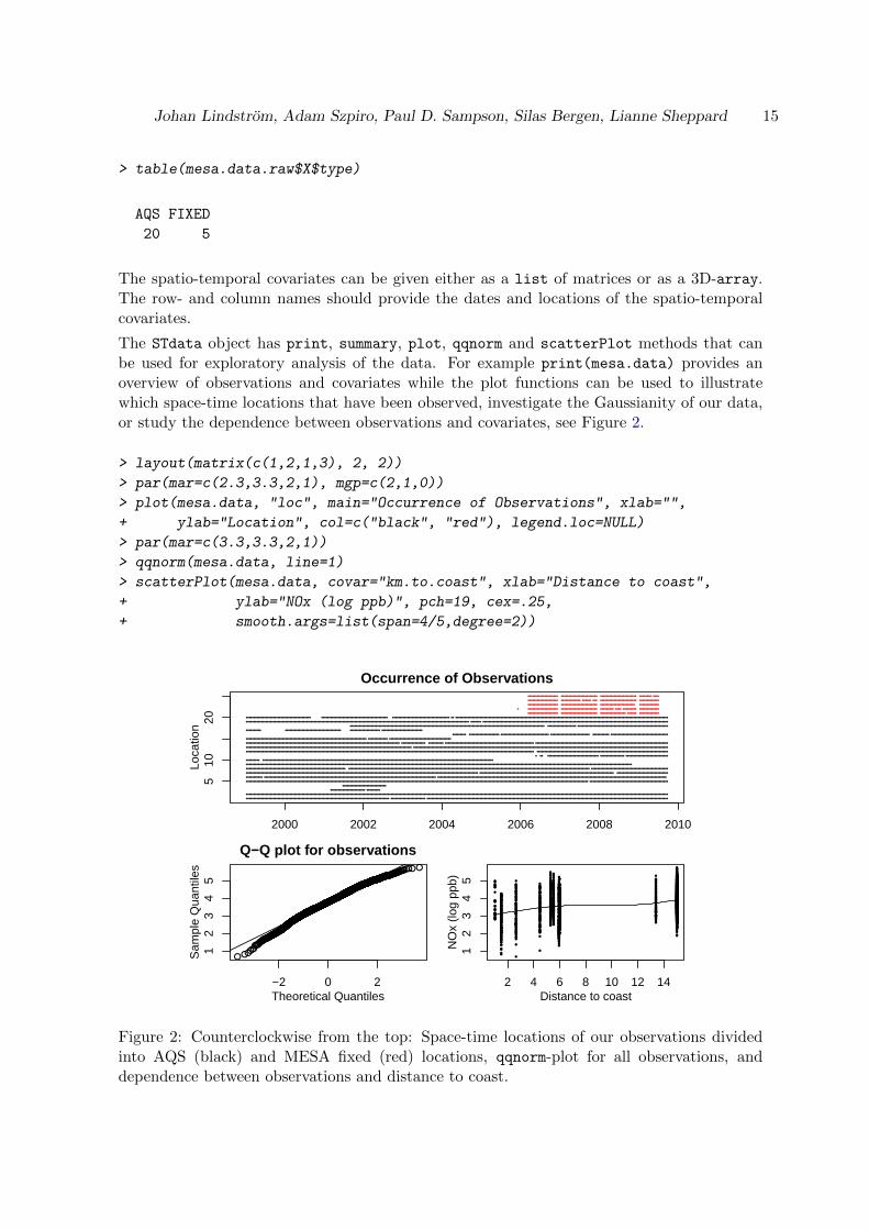
The STdata object has print, summary, plot, qqnorm and scatterPlot methods that canbe used for exploratory analysis of the data. For example print(mesa.data) provides anoverview of observations and covariates while the plot functions can be used to illustratewhich space-time locations that have been observed, investigate the Gaussianity of our data,or study the dependence between observations and covariates, see Figure 2.

> layout(matrix(c(1,2,1,3), 2, 2))

> par(mar=c(2.3,3.3,2,1), mgp=c(2,1,0))

> plot(mesa.data, "loc", main="Occurrence of Observations", xlab="",

+ ylab="Location", col=c("black", "red"), legend.loc=NULL)

> par(mar=c(3.3,3.3,2,1))

> qqnorm(mesa.data, line=1)

> scatterPlot(mesa.data, covar="km.to.coast", xlab="Distance to coast",

+ ylab="NOx (log ppb)", pch=19, cex=.25,

+ smooth.args=list(span=4/5,degree=2))

2000 2002 2004 2006 2008 2010

510

20

Occurrence of Observations

Loca

tion

● ● ● ● ● ● ● ● ● ● ● ● ● ● ● ● ● ● ● ● ● ● ● ● ● ● ● ● ● ● ● ● ● ● ● ● ● ● ● ● ● ● ● ● ● ● ● ● ● ● ● ● ● ● ● ● ● ● ● ● ● ● ● ● ● ● ● ● ● ● ● ● ● ● ● ● ● ● ● ● ● ● ● ● ● ● ● ● ● ● ● ● ● ● ● ● ● ● ● ● ● ● ● ● ● ● ● ● ● ● ● ● ● ● ● ● ● ● ● ● ● ● ● ● ● ● ● ● ● ● ● ● ● ● ● ● ● ● ● ● ● ● ● ● ● ● ● ● ● ● ● ● ● ● ● ● ● ● ● ● ● ● ● ● ● ● ● ● ● ● ● ● ● ● ● ● ● ● ● ● ● ● ● ● ● ● ● ● ● ● ● ● ● ● ● ● ● ● ● ● ● ● ● ● ● ● ● ● ● ● ● ● ● ● ● ● ● ● ● ● ● ● ● ● ● ● ● ● ● ● ● ● ● ● ● ● ● ● ● ● ● ● ● ● ● ● ● ● ● ● ● ● ● ● ● ● ● ● ● ● ● ● ● ● ● ● ● ● ● ● ● ● ● ● ● ● ● ●

● ● ● ● ● ● ● ● ● ● ● ● ● ● ● ● ● ● ● ● ● ● ● ● ● ● ● ● ● ● ● ● ● ● ● ● ● ● ● ● ● ● ● ● ● ● ● ● ● ● ● ● ● ● ● ● ● ● ● ● ● ● ● ● ● ● ● ● ● ● ● ● ● ● ● ● ● ● ● ● ● ● ● ● ● ● ● ● ● ● ● ● ● ● ● ● ● ● ● ● ● ● ● ● ● ● ● ● ● ● ● ● ● ● ● ● ● ● ● ● ● ● ● ● ● ● ● ● ● ● ● ● ● ● ● ● ● ● ● ● ● ● ● ● ● ● ● ● ● ● ● ● ● ● ● ● ● ● ● ● ● ● ● ● ● ● ● ● ● ● ● ● ● ● ● ● ● ● ● ● ● ● ● ● ● ● ● ● ● ● ● ● ● ● ● ● ● ● ● ● ● ● ● ● ● ● ● ● ● ● ● ● ● ● ● ● ● ● ● ● ● ● ● ● ● ● ● ● ● ● ● ● ● ● ● ● ● ● ● ● ● ● ● ● ● ● ● ● ● ● ● ● ● ● ● ● ● ● ● ● ● ● ● ● ● ● ● ● ● ● ● ● ● ● ● ● ● ● ● ●

● ● ● ● ● ● ● ● ● ● ● ● ● ● ● ● ● ● ● ● ● ● ● ● ● ● ● ● ● ● ● ●

● ● ● ● ● ● ● ● ● ● ● ● ● ● ● ● ● ● ● ● ● ● ● ● ● ● ● ● ●

● ● ● ● ● ● ● ● ● ● ● ● ● ● ● ● ● ● ● ● ● ● ● ● ● ● ● ● ● ● ● ● ● ● ● ● ● ● ● ● ● ● ● ● ● ● ● ● ● ● ● ● ● ● ● ● ● ● ● ● ● ● ● ● ● ● ● ● ● ● ● ● ● ● ● ● ● ● ● ● ● ● ● ● ● ● ● ● ● ● ● ● ● ● ● ● ● ● ● ● ● ● ● ● ● ● ● ● ● ● ● ● ● ● ● ● ● ● ● ● ● ● ● ● ● ● ● ● ● ● ● ● ● ● ● ● ● ● ● ● ● ● ● ● ● ● ● ● ● ● ● ● ● ● ● ● ● ● ● ● ● ● ● ● ● ● ● ● ● ● ● ● ● ● ● ● ● ● ● ● ● ● ● ● ● ● ● ● ● ● ● ● ● ● ● ● ● ● ● ● ● ● ● ● ● ● ● ● ● ● ● ● ● ● ● ● ● ● ● ● ● ● ● ● ● ● ● ● ● ● ● ● ● ● ● ● ● ● ● ● ● ● ● ● ● ● ● ● ● ● ● ● ● ● ● ● ● ● ● ● ● ● ● ● ● ● ● ● ● ● ● ● ● ● ● ● ● ● ●

● ● ● ● ● ● ● ● ● ● ● ● ● ● ● ● ● ● ● ● ● ● ● ● ● ● ● ● ● ● ● ● ● ● ● ● ● ● ● ● ● ● ● ● ● ● ● ● ● ● ● ● ● ● ● ● ● ● ● ● ● ● ● ● ● ● ● ● ● ● ● ● ● ● ● ● ● ● ● ● ● ● ● ● ● ● ● ● ● ● ● ● ● ● ● ● ● ● ● ● ● ● ● ● ● ● ● ● ● ● ● ● ● ● ● ● ● ● ● ● ● ● ● ● ● ● ● ● ● ● ● ● ● ● ● ● ● ● ● ● ● ● ● ● ● ● ● ● ● ● ● ● ● ● ● ● ● ● ● ● ● ● ● ● ● ● ● ● ● ● ● ● ● ● ● ● ● ● ● ● ● ● ● ● ● ● ● ● ● ● ● ● ● ● ● ● ● ● ● ● ● ● ● ● ● ● ● ● ● ● ● ● ● ● ● ● ● ● ● ● ● ● ● ● ● ● ● ● ● ● ● ● ● ● ● ● ● ● ● ● ● ● ● ● ● ● ● ● ● ● ● ● ● ● ● ● ● ● ● ● ● ● ● ● ● ● ● ● ● ● ● ● ● ● ● ● ●

● ● ● ● ● ● ● ● ● ● ● ● ● ● ● ● ● ● ● ● ● ● ● ● ● ● ● ● ● ● ● ● ● ● ● ● ● ● ● ● ● ● ● ● ● ● ● ● ● ● ● ● ● ● ● ● ● ● ● ● ● ● ● ● ● ● ● ● ● ● ● ● ● ● ● ● ● ● ● ● ● ● ● ● ● ● ● ● ● ● ● ● ● ● ● ● ● ● ● ● ● ● ● ● ● ● ● ● ● ● ● ● ● ● ● ● ● ● ● ● ● ● ● ● ● ● ● ● ● ● ● ● ● ● ● ● ● ● ● ● ● ● ● ● ● ● ● ● ● ● ● ● ● ● ● ● ● ● ● ● ● ● ● ● ● ● ● ● ● ● ● ● ● ● ● ● ● ● ● ● ● ● ● ● ● ● ● ● ● ● ● ● ● ● ● ● ● ● ● ● ● ● ● ● ● ● ● ● ● ● ● ● ● ● ● ● ● ● ● ● ● ● ● ● ● ● ● ● ● ● ● ● ● ● ● ● ● ● ● ● ● ● ● ● ● ● ● ● ● ● ● ● ● ● ● ● ● ● ● ● ● ● ● ● ● ● ● ● ● ● ● ● ● ● ● ● ●

● ● ● ● ● ● ● ● ● ● ● ● ● ● ● ● ● ● ● ● ● ● ● ● ● ● ● ● ● ● ● ● ● ● ● ● ● ● ● ● ● ● ● ● ● ● ● ● ● ● ● ● ● ● ● ● ● ● ● ● ● ● ● ● ● ● ● ● ● ● ● ● ● ● ● ● ● ● ● ● ● ● ● ● ● ● ● ● ● ● ● ● ● ● ● ● ● ● ● ● ● ● ● ● ● ● ● ● ● ● ● ● ● ● ● ● ● ● ● ● ● ● ● ● ● ● ● ● ● ● ● ● ● ● ● ● ● ● ● ● ● ● ● ● ● ● ● ● ● ● ● ● ● ● ● ● ● ● ● ● ● ● ● ● ● ● ● ● ● ● ● ● ● ● ● ● ● ● ● ● ● ● ● ● ● ● ● ● ● ● ● ● ● ● ● ● ● ● ● ● ● ● ● ● ● ● ● ● ● ● ● ● ● ● ● ● ● ● ● ● ● ● ● ● ● ● ● ● ● ● ● ● ● ● ● ● ● ● ● ● ● ● ● ● ● ● ● ● ● ● ● ● ● ● ● ● ● ● ● ● ● ● ● ● ● ● ● ● ● ● ● ● ● ● ● ● ●

● ● ● ● ● ● ● ● ● ● ● ● ● ● ● ● ● ● ● ● ● ● ● ● ● ● ● ● ● ● ● ● ● ● ● ● ● ● ● ● ● ● ● ● ● ● ● ● ● ● ● ● ● ● ● ● ● ● ● ● ● ● ● ● ● ● ● ● ● ● ● ● ● ● ● ● ● ● ● ● ● ● ● ● ● ● ● ● ● ● ● ● ● ● ● ● ● ● ● ● ● ● ● ● ● ● ● ● ● ● ● ● ● ● ● ● ● ● ● ● ● ● ● ● ● ● ● ● ● ● ● ● ● ● ● ● ● ● ● ● ● ● ● ● ● ● ● ● ● ● ● ● ● ● ● ● ● ● ● ● ● ● ● ● ● ● ● ● ● ● ● ● ● ● ● ● ● ● ● ● ● ● ● ● ● ● ● ● ● ● ● ● ● ● ● ● ● ● ● ● ● ● ● ● ● ● ● ● ● ● ● ● ● ● ● ● ● ● ● ● ● ● ● ● ● ● ● ● ● ● ● ● ● ● ● ● ● ● ● ● ● ● ● ● ● ● ● ● ● ● ● ● ● ● ● ●

● ● ● ● ● ● ● ● ● ● ● ● ● ● ● ● ● ● ● ● ● ● ● ● ● ● ● ● ● ● ● ● ● ● ● ● ● ● ● ● ● ● ● ● ● ● ● ● ● ● ● ● ● ● ● ● ● ● ● ● ● ● ● ● ● ● ● ● ● ● ● ● ● ● ● ● ● ● ● ● ● ● ● ● ● ● ● ● ● ● ● ● ● ● ● ● ● ● ● ● ● ● ● ● ● ● ● ● ● ● ● ● ● ● ● ● ● ● ● ● ● ● ● ● ● ● ● ● ● ● ● ● ● ● ● ● ● ● ● ● ● ● ● ● ● ● ● ● ● ● ● ● ● ● ● ● ● ● ● ● ● ●

● ● ● ● ● ● ● ● ● ● ● ● ● ● ● ● ● ● ● ● ● ● ● ● ● ● ● ● ● ● ● ● ● ● ● ● ● ● ● ● ● ● ● ● ● ● ● ● ● ● ● ● ● ● ● ● ● ● ● ● ● ● ● ● ● ● ● ● ● ● ● ● ● ● ● ● ● ● ● ● ●

● ● ● ● ● ● ● ● ● ● ● ● ● ● ● ● ● ● ● ● ● ● ● ● ● ● ● ● ● ● ● ● ● ● ● ● ● ● ● ● ● ● ● ● ● ● ● ● ● ● ● ● ● ● ● ● ● ● ● ● ● ● ● ● ● ● ● ● ● ● ● ● ● ● ● ● ● ● ● ● ● ● ● ● ● ● ● ● ● ● ● ● ● ● ● ● ● ● ● ● ● ● ● ● ● ● ● ● ● ● ● ● ● ● ● ● ● ● ● ● ● ● ● ● ● ● ● ● ● ● ● ● ● ● ● ● ● ● ● ● ● ● ● ● ● ● ● ● ● ● ● ● ● ● ● ● ● ● ● ● ● ● ● ● ● ● ● ● ● ● ● ● ● ● ● ● ● ● ● ● ● ● ● ● ● ● ● ● ● ● ● ● ● ● ● ● ● ● ● ● ● ● ● ● ● ● ● ● ● ● ● ● ● ● ● ● ● ● ● ● ● ● ● ● ● ● ● ● ● ● ● ● ● ● ● ● ● ● ● ● ● ● ● ● ● ● ● ● ● ● ● ● ● ● ● ● ● ● ● ● ● ● ● ● ● ● ● ● ● ● ● ● ● ● ● ● ● ●

● ● ● ● ● ● ● ● ● ● ● ● ● ● ● ● ● ● ● ● ● ● ● ● ● ● ● ● ● ● ● ● ● ● ● ● ● ● ● ● ● ● ● ● ● ● ● ● ● ● ● ● ● ● ● ● ● ● ● ● ● ● ● ● ● ● ● ● ● ● ● ● ● ● ● ● ● ● ● ● ● ● ● ● ● ● ● ● ● ● ● ● ● ● ● ● ● ● ● ● ● ● ● ● ● ● ● ● ● ● ● ● ● ● ● ● ● ● ● ● ● ● ● ● ● ● ● ● ● ● ● ● ● ● ● ● ● ● ● ● ● ● ● ● ● ● ● ● ● ● ● ● ● ● ● ● ● ● ● ● ● ● ● ● ● ● ● ● ● ● ● ● ● ● ● ● ● ● ● ● ● ● ● ● ● ● ● ● ● ● ● ● ● ● ● ● ● ● ● ● ● ● ● ● ● ● ● ● ● ● ● ● ● ● ● ● ● ● ● ● ● ● ● ● ● ● ● ● ● ● ● ● ● ● ● ● ● ● ● ● ● ● ● ● ● ● ● ● ● ● ● ● ● ● ● ● ● ● ● ● ● ● ● ● ● ● ● ● ● ● ● ● ● ● ● ● ● ● ●

● ● ● ● ● ● ● ● ● ● ● ● ● ● ● ● ● ● ● ● ● ● ● ● ● ● ● ● ● ● ● ● ● ● ● ● ● ● ● ● ● ● ● ● ● ● ● ● ● ● ● ● ● ● ● ● ● ● ● ● ● ● ● ● ● ● ● ● ● ● ● ● ● ● ● ● ● ● ● ● ● ● ● ● ● ● ● ● ● ● ● ● ● ● ● ● ● ● ● ● ● ● ● ● ● ● ● ● ● ● ● ● ● ● ● ● ● ● ● ● ● ● ● ● ● ● ● ● ● ● ● ● ● ● ● ● ● ● ● ● ● ● ● ● ● ● ● ● ● ● ● ● ● ● ● ● ● ● ● ● ● ● ● ● ● ● ● ● ● ● ● ● ● ● ● ● ● ● ● ● ● ● ● ● ● ● ● ● ● ● ● ● ● ● ● ● ● ● ● ● ● ● ● ● ● ● ● ● ● ● ● ● ● ● ● ● ● ● ● ● ● ● ● ● ● ● ● ● ● ● ● ● ● ● ● ● ● ● ● ● ● ● ● ● ● ● ● ● ● ● ● ● ● ● ● ● ● ● ● ● ● ● ● ● ● ● ● ● ● ● ● ● ● ● ●

● ● ● ● ● ● ● ● ● ● ● ● ● ● ● ● ● ● ● ● ● ● ● ● ● ● ● ● ● ● ● ● ● ● ● ● ● ● ● ● ● ● ● ● ● ● ● ● ● ● ● ● ● ● ● ● ● ● ● ● ● ● ● ● ● ● ● ● ● ● ● ● ● ● ● ● ● ● ● ● ● ● ● ● ● ● ● ● ● ● ● ● ● ● ● ● ● ● ● ● ● ● ● ● ● ● ● ● ● ● ● ● ● ● ● ● ● ● ● ● ● ● ● ● ● ● ● ● ● ● ● ● ● ●

● ● ● ● ● ● ● ● ● ● ● ● ● ● ● ● ● ● ● ● ● ● ● ● ● ● ● ● ● ● ● ● ● ● ● ● ● ● ● ● ● ● ● ● ● ● ● ● ● ● ● ● ● ● ● ● ● ● ● ● ● ● ● ● ● ● ● ● ● ● ● ● ● ● ● ● ● ● ● ● ● ● ● ● ● ● ● ● ● ● ● ● ● ● ● ● ● ● ● ● ● ● ● ● ● ● ● ● ● ● ● ● ● ● ● ● ● ● ● ● ● ● ● ● ● ● ● ● ● ● ● ● ● ● ● ●

● ● ● ● ● ● ● ● ● ● ● ● ● ● ● ● ● ● ● ● ● ● ● ● ● ● ● ● ● ● ● ● ● ● ● ● ● ● ● ● ● ● ● ● ● ● ● ● ● ● ● ● ● ● ● ● ● ● ● ● ● ● ● ● ● ● ● ● ● ● ● ● ● ● ● ● ● ● ● ● ● ● ● ● ● ● ● ● ● ● ● ● ● ●

● ● ● ● ● ● ● ● ● ● ● ● ● ● ● ● ● ● ● ● ● ● ● ● ● ● ● ● ● ● ● ● ● ● ● ● ● ● ● ● ● ● ● ● ● ● ● ● ● ● ● ● ● ● ● ● ● ● ● ● ● ● ● ● ● ● ● ● ● ● ● ● ● ● ● ● ● ● ● ● ● ● ● ● ● ● ● ● ● ● ● ● ● ● ● ● ● ● ● ● ● ● ● ● ● ● ● ● ● ● ● ● ● ● ● ● ● ● ● ● ● ● ● ● ● ● ● ● ● ● ● ● ● ● ● ● ● ● ● ● ● ● ● ● ● ● ● ● ● ● ● ● ● ● ● ● ● ● ● ● ● ● ● ● ● ● ● ● ● ● ● ● ● ● ● ● ● ● ● ● ● ● ● ● ● ● ● ● ● ● ● ● ● ● ● ● ● ● ● ● ● ● ● ● ● ● ● ●

● ● ● ● ● ● ● ● ● ● ● ● ● ● ● ● ● ● ● ● ● ● ● ● ● ● ● ● ● ● ● ● ● ● ● ● ● ● ● ● ● ● ● ● ● ● ● ● ● ● ● ● ● ● ● ● ● ● ● ● ● ● ● ● ● ● ● ● ● ● ● ● ● ● ● ● ● ● ● ● ● ● ● ● ● ● ● ● ● ● ● ● ● ● ● ● ● ● ● ● ● ● ● ● ● ● ● ● ● ● ● ● ● ● ● ● ● ● ● ● ● ● ● ● ● ● ● ● ● ● ● ● ● ● ● ● ● ● ● ● ● ● ● ● ● ● ● ● ● ● ● ● ● ● ● ● ● ● ● ● ● ● ● ● ● ● ● ● ● ● ● ● ● ● ● ● ● ● ● ● ● ● ● ● ● ● ● ● ● ● ● ● ● ● ● ● ● ● ● ● ● ● ● ● ● ● ● ● ● ● ● ● ● ● ● ● ● ● ● ● ● ● ● ● ● ● ● ● ● ● ● ● ● ● ● ● ● ● ● ● ● ● ● ● ● ● ● ● ● ● ● ● ● ● ● ● ● ● ● ● ● ● ● ● ● ● ● ● ● ● ● ● ● ● ● ● ● ●

● ● ● ● ● ● ● ● ● ● ● ● ● ● ● ● ● ● ● ● ● ● ● ● ● ● ● ● ● ● ● ● ● ● ● ● ● ● ● ● ● ● ● ● ● ● ● ● ● ● ● ● ● ● ● ● ● ● ● ● ● ● ● ● ● ● ● ● ● ● ● ● ● ● ● ● ● ● ● ● ● ● ● ● ● ● ● ● ● ● ● ● ● ● ● ● ● ● ● ● ● ● ● ● ● ● ● ● ● ● ● ● ● ● ● ● ● ● ● ● ● ● ● ● ● ● ● ● ● ● ● ● ● ● ● ● ● ● ● ● ● ● ● ● ● ● ● ● ● ● ● ● ● ● ● ● ● ● ● ● ● ● ● ● ● ● ● ● ● ● ● ● ● ● ● ● ● ● ● ● ● ● ● ● ● ● ● ● ● ● ● ● ● ● ● ● ● ● ● ● ● ● ● ● ● ● ● ● ● ● ● ● ● ● ● ● ● ● ● ● ● ● ● ● ● ● ● ● ● ● ● ● ● ● ● ● ● ● ● ● ● ● ● ● ● ● ● ● ● ● ● ● ● ● ● ● ● ● ● ● ● ● ● ● ● ● ● ●

● ● ● ● ● ● ● ● ● ● ● ● ● ● ● ● ● ● ● ● ● ● ● ● ● ● ● ● ● ● ● ● ● ● ● ● ● ● ● ● ● ● ● ● ● ● ● ● ● ● ● ● ● ● ● ● ● ● ● ● ● ● ● ● ● ● ● ● ● ● ● ● ● ● ● ● ● ● ● ●

● ● ● ● ● ● ● ● ● ● ● ● ● ● ● ● ● ● ● ● ● ● ● ● ● ● ● ● ● ● ● ● ● ● ● ● ● ● ● ● ● ● ● ● ● ● ● ● ● ● ● ● ● ● ● ● ● ● ● ● ● ● ● ● ● ● ● ● ● ● ● ● ● ● ● ● ● ● ● ●

● ● ● ● ● ● ● ● ● ● ● ● ● ● ● ● ● ● ● ● ● ● ● ● ● ● ● ● ● ● ● ● ● ● ● ● ● ● ● ● ● ● ● ● ● ● ● ● ● ● ● ● ● ● ● ● ● ● ● ● ● ● ● ● ● ● ● ● ● ● ● ● ● ● ● ● ● ● ● ●

● ● ● ● ● ● ● ● ● ● ● ● ● ● ● ● ● ● ● ● ● ● ● ● ● ● ● ● ● ● ● ● ● ● ● ● ● ● ● ● ● ● ● ● ● ● ● ● ● ● ● ● ● ● ● ● ● ● ● ● ● ● ● ● ● ● ● ● ● ● ● ● ● ● ● ● ● ● ●

● ● ● ● ● ● ● ● ● ● ● ● ● ● ● ● ● ● ● ● ● ● ● ● ● ● ● ● ● ● ● ● ● ● ● ● ● ● ● ● ● ● ● ● ● ● ● ● ● ● ● ● ● ● ● ● ● ● ● ● ● ● ● ● ● ● ● ● ● ● ● ● ● ● ● ● ● ● ● ●

●

●●●●●

●

●

●●●●●

●●●

●●

●●●●●●●

●

●●●

●●●●●●●●●●●

●●●●●●

●●●

●

●

●

●●

●●●

●

●●

●●●●●

●●●●

●

●●●●●

●●●●

●●●●●●●●●●●●●●●

●

●●●●●

●●

●

●●

●●

●●●●●

●●●

●●●●●●

●●●

●●●

●●

●●●

●

●

●●●

●

●●

●●

●

●●

●

●

●●

●

●●●●

●

●

●●

●●

●

●●●

●●

●●●●

●●

●

●●●●●●

●●●

●●●

●●

●●●●●●●●

●●

●●

●

●●●●

●●●●

●●

●

●●●●●

●●●●●●

●●●●●●●●

●●●

●

●

●●

●●●●●●●

●●●●●●

●●

●

●

●

●●

●●●

●

●

●

●●

●●●●

●●●●●●

●●●

●

●●●

●●

●●●●●

●●●●●●

●●

●●●●●

●●

●●●

●●●●●●●

●●●●●

●●●●●●●●

●●●

●●

●●●

●

●●●●●

●●●●●●

●●●

●●●

●●●●

●●●●

●●●●●

●●●●

●●●● ●

●●●●●

●

●

●●●●●●

●●●

●●●●●●

●●●●●●●●●●

●●●

●●

●

●

●●●

●●

●●●●●●●●●●

● ●●●●

●

●●●

●●

●●●●

●●●●●●

●●●●

●●●●●

●●●●

●●

●●●●●●●

●●●●

●●●

●●

●●●

●●

●●●●

●

●●●●●●●

●●●●●●●

●●●

●●

●●●●

●

●●●●

●●●●●

●●●●●●●●

●

●●

●●

●●●●

●

●●●

●●

●●●●●●●

●●●●

●●

●

●●●●

●●●●

●●●

●●●●

●●

●●●●●

●●

●●

●●●

●●●●●

●

●●●●

●●●

●●●●

●●●

●●●

●●●●

●●

●

●●●

●●●

●●

●●

●●

●●

●●●●

●●●●● ●●●

●●●●●●●●●

●●

●

●●●●

●●

●

●●●

●●

●

●●●●

●●●

●●

●●●●

●●●●

●

●●●●

●

●●

●●●

●●●

●

●●●●●●

●●●

●●●●●

●

●●●

●

●●

●●

●●

●●●

●●●

●●●

●

●●●●●

●●●●●

●●●

●●

●● ●●●

●

●

●●

●

●●●

●●

●●

●●●●●

●

●●

●●●●●

●●●

●

●

●

●

●●

●●

●●●●●●●●●●●●

●●

●●

●●●●

●●●●

●●●●

●●●●●●●●●

●●●

●●●

●

●●●●

●

●●●●

●

●

●●●●

●

●

●

●●●●

●●

●●●●

●●●●●

●●

●

●

●

●●●●●

●●

●●●●●

●●●●●●●

●●

●

●●● ●

●●

●

●●●●●●

●●●

●●

● ●●●●●

●●

●●●●●●●●●●●●●

●●●

●●●

●●

●●

●

●

●●●●

●●

●●●●●●●

●●●●

●

●●●●

●●

●●●●

●●

●●

●●

●●●●●●●●

●●

●●●

●

●●

●●

●●●

●●

●●●●

●●

●●

●●●●●●

●

●●●●

● ●●

●●●●

●●

●●●

●●

●●●●●

●

●●●●●

●●

●

●

●●●●●●

●●●●

●●●●●

●●●●●●

●●●●●●●

●

●●●●●●●

●●●

●●

●●●●

●●●●●●●●

●●●

●●●●

●●

●●●●

●●●●●

●●

●●●●

●

●

●●●●

●●●

●●●

●●●●●●●●

●●

●●●●

●●

●

●

● ●●●●●

●●●

●●●

●●

●●●●

●●●

●

●●●●●●

●●●

●●

● ●●●●

●●●

●●●●●●●●●

●●●●

●●●●●

●

●●●

●●

●

●●●

●●

●

●

●●●●

●●●● ●

●

●

●●●●

●●

●●●●●

●●

●

●●

●●●●●

●●●

●●●●

●

●

●● ●

●● ●●

●●

●●

●●●●

●●

●●

●●●●●

● ●●

●●

●●●●●●●●

●●

●●●●●

●●●

●●●●●●●

●

●

●●

●●●●●

●●●●

●●●●●

●●

●●●

●●●

●●●●●●

●●

●●

●●●●

●●

●●

●●

●●

●●●●●●●●

●●●

●●●●

●●

●●●●

●●●●●

●●

●●●●

●

●

●●●●

●●

●

●●●●●●

●

●●

●●

●

●●●

●●

●

●

●●●●●

●●●●

●●

●

●●

●

●

●●●

●●●

●●●●●●●●●

●●●

●●●

●●●●

●

●●●

●●●●●●●●

●●●●●●●

●

●●

●

●

●

●

●●●●

●●

●●●

●●●●

●

●●●●

●●

●●●●

●●●●

●

●●●●●●●●●●

●●●●

●●●

●●●

●●●●

●●

●●●●

●●●

●●●●●●●●

●●●●●●●

●●

●●●

●●●●

●●

●●

●●●●

●

●●●●●

●

●●

●

●●●●

●●

●●●

●●●●●●

●●●●

●●

●●●

●●●●●

●●●●

●●●●

●●

●●

●●●

●

●●●

●●●●●

●●

●●

●●●●●

●●●●

●●●●

●●

●●●●●

●

●

●●●

●●●●●

●●●

●●●●●●

●

●

●●●●●●●

●

●●●●●●●●●●

●●●

●●

●●●●

●●●●

●●●●●●●●●

●●

●●

●●

●●

●●

●●●●●●●●●●●●●

●●●●●

●

●●

●●

●●

●●●

●●

●

●●

●●●●●●●●●

●●●

●●

●●●●●

●●

●●●

●●●●●●●●●●●

●●●●

●

●●●●●

●●

●●

●●●

●●

●●●●●●●●●●

●●● ● ●●●●●●

●●●

●●

●●●●

●●●●●●

●●●

●●●●

●

●●

●●●●●●●

●●●●●●●●●

●●●●●●●●●

●●●

●●●●●●●●●●

●●●●●●

●●●●●●●●

●●●●

●●●

●●●●●●●●●

●●

●

●● ●●

●●

●

●●●●●●

●●●●●●●●●●●

●●

●●

● ●

●●●

●●

●●●

●●●●●

● ●●

● ●●

● ●

●●●●●●●●

●●●●●●●●

●●●

●●●

●●

●●●

●●

●●

●

●●

●●●

●●●

●●●

●●●●

●●

●●●●●

●●●

●●

●●●●●●●●●

●●●●

●

●●

●

●●

●●

●●●●

●●●●●●●●

●●●●●

●●●●

●● ●●●●

●●●●

●●

●●●

●●●●

●●●●

●●●● ●

●

●●

●●●●●

●●●●

●●

●●●●●●●●●

●●●

●●●

●●

●●●●

●●●●●

●

●●●●

●

●

●●

●●

●●

●●

●●

●●●●

●●●

●●

●

●●●

●●

●●

●●●●

●●●●

●●●●

●●

●

●●●

●●●●●

●●●

●●●●●

●●●●●● ● ●●●

●

● ●●●●●●●●●●●●●●●

●●●

●●

●●

●●

●●●●●●

●●●

●●●●

●●●●

●

●●●

●●

●●●●

●●

●●●●●

●●●●●●●

●●

●●

●●●●

●●

●●●

●

●●●●

●●●●

●●●●

●●●●

●

●●●●●● ●

●●●●●

●●●

●●●●

●●●●●●

●●●● ●●●

●

●

●●●●●●

●●●●

●●●●●●

●●●●●

●●●●●●●●

●●●●●●●●

●●

●●●

●

●●●●●●●●●●

●●

●●●●●

●●●●●●●●●

●●●●●●●

●●

●●●●●

● ●●●●●●●● ●

●●●

●●

●●●●

●●

●

●●●●●●

●●●●

●●

●●

●

●

●●●

●●

●

●●●●

●●

●●●●

●●

●●●●

●●

●●

●●●●●●

●●●

●●●●

●●●●●●

●●

●

●●

●

●●●

●●●

●●●

●●●●

●●●●

●

●●●●

●●

●●●●

●●

●●●●

●●●●●●

●●●●

●●●

●●

●●

●●

●●

●●

●●●

●●●●●●●●●●

●

●●●

●●

●●●●●

●●

●●●●

●●●●

●●●●●●●●

●●●●

●

●

●

●●●

●●

●●●●

●●●●

●●

●

●●●●

●●●●●●●●

● ●●●●●●

●●●

●●

●●●

●●

●●●●●●●●●●

●●●●●●

●●●●●●●●●

●●●●●

●●

●

●●●●

●●●●●

●●●●●●●●●

●●

●●●●

●●

●

●

● ●

●●●●●●

●●●●●

●●

●●

●●●●

●●

●●●●●●●●●

●●

●●

●●

●●

● ●

●●

●●

●●●●●●

●●●●●●

●●●

●●

● ●●

●●●

●●

●●●

●●

●●●●●●

●●●●●●●

●●●●●

●●●

●●●●●●●●●●●●●

●●●●●

●●●●●●

●●

●●

●●

●●●●●●●●●

●●●●

●●●●●●

●●

●

●●●●●●●●●

●●●●

●●●●●

●

●●

●●●●●●●●●●●●●●●●

●●●●

●●●●●●●●

●●●●

●●●●●●●●●●●

●●●●●●●●

●●

●●

●●●

●●●●●●

●●●●●

●●

●●●●

●

●

●

●●●●●

●●●●●●●●

●●

●●

●●

●

●●●

●●

●●

●●●●

●●●●

●

●●●

●●

●

●●●●

●●●

●●

●●

●●●

●●●●●

● ●●●●

●●●

●●●●

●●●●●

●●●

●●●●

●●

●

●●

●●●

●●●●

●●●

●

●

●

●●●●

●●●

●●

●●●

●

●●

●●●●●

●●

●

●

●●●●

●●●

●●●

●

●

●

●●●●●

●●

●●

●●

●●●●

●●

●

●

●●●●

●

●

●●● ●●●

●●●●

●●

●

●

●

●●

●●

●

●●

●

●●●●●

●

●●

●●●●

●

●●●

●●

●●●

●●

●●●●

●●●●●●●●

●●●

●●

●●●●●

●●

●

●●

●●●●●●●

●●●

●●

●●●

●

●●●●●

●●●●

●

●●●

●

●

●

●

●●●●

●●

●●●

●●●

●●

●

●●●

●

●●●

●●

●●

●●●

●●

●●

●●●●●

●●

●

●●

●●

●●●

●

●●

●

●●●●●●

●●●●●●● ●●●

●●●

●●

●●●

●●●

●●

●●

●

●●

●●●

●

●

●●

●●

●●●●

●●

●●

●●●●●●●●

●●

●●●●

●

●●

●●

● ●●

●●●●

●●

●●

●●●

●●

●●

●●

●●●●

●●

●●

●●●

●●●

●●●●●

●●●●

●

●●

●●

● ●●

●●●●

●●

●●

●●●●

●●●●

●

●●●●●●●

●●●●

●●

●

●

●

●●●

●●●●

●●

●●

●●●

●●

●

●●

●●●●●

●●●

●●●●●●

●●

●●●●

●●●●●●●●

●●●

●●●●

●●●●

●●●

●●●●●

●●●●

●●●

●●●

●●●●●

●●●

●●

●●

●●●

●

●

●●

●●●

●●

●●

●●

●●●●●

●

●●

●●

●

●●●●

●

●

●

●●●●

●●●●

●●●●

●

●●

●●●●

●●●

●

●●

●●●●●●●●●

●●

●●

●

●●

●

●●●●

●●

●●●

●●●

●●●●

●●

●

●●

●●●●●●

●●

●●

●

●

●●●●

●●

●●●●

●●●

●

●●

●●●●

●

●

●●

●●●

●●●●●●

●●

●●●

●

●

●●

●●●

●●

●●

●●

●●●●●●●●

●●●●

●

●●

●●●

●●

●●●●

●●

●

●

●●●●

●●●●

●

● ●●●●

●●

●

●●

●●●●

●●●●●

●●●●

●●

●●●●

●●●●●

●●●

●●●

●●

●●●●●

●●

●●●●

●●●

●●●●●

●●

●●

●●●

●●●●●●

●●●

●●

●●

●●●

●●

●

●

●●

●●●

●●

●●

●●●●●●

●●

●●●

●●●

●●

●

●

●●●●

●●●●

●●●●

●

●●

●●

●●

●●●

●

●●●●●●●●

●●●

●●

●● ● ●●

●

●●●●

●●●

●●●●●

●●●●

●●

●●

●

●●●

●●●

●●●●●●●●●

●●●●

●●

●●●●●

●●●

●●●●●●●●●

●

●●

●

●●

●●

●●

●

●●

●●●●●

●●●●●●●●

●●

●●●●

●●●●●●

●●

●●●

●●●●●

●●

●●●

●●●●●

●

●●

●●●●●●●●

●●●

●●●●●

●●●●

●●●●●●●

●

●●●●

●●●●●

●●

●●●

●●

●●●●●●●●

●●●

●●

●●

●●●●●●

●●●●●

●●

●●●●

●

●

●

●●●●●

●●●

●●●●●●

●●●

●●

●●

●●●

●

●●

●●●●

●●●●●●

●●

●●

●●●

●●●●●●●

●●●

●●●

●

●●● ●●●

●●●●

●●●

●●●●●●

●●●●●

●●

●●●

●●

●●●●●

●●

●●●●●●●

●●●●

●●●

●

●●

●●●

●●●●●●

●

●●●●●●●●●●●●●●

●●

●●●●●●●

●●●●●●●●●

●●●●● ●●●

●●

●●●

●●

●●●●●●

●●●●●●●●

●●

●

●●

●●●●

●●●●●●●●●●●●

●

●

●●●●●

●

●

●●

●●

●●

●●●●

●●

●●

●●●

●

●●●●

●

●●

●●

●

●

●

●●●

●

●●●

●●●

●●●●●

●●●●

●

●

●●●

●●

●

●●●

●●●

●

●

●●●

●●●●

●●●●●●●

●

●●●●

●●●

●●●●

●●

●●●●

●●

●●●

●●

●●

●●●

●●

●

●●●

●●●

●●●

●●●●●●

●

●●

●●

●

●

●●

●●

●●●●

●●

●●●

●●●

●

●

●

●

●●●●

●

●●

●●

●●

●●●●

●●●

●●●●

●

●●●●

●

●●●●

●

●

●

●●●

●●

●●●

●●●●●●

●●●●

●●

●

●●●

●●

●●

●●●●

●●

●●

●●

−2 0 2

12

34

5

Q−Q plot for observations

Theoretical Quantiles

Sam

ple

Qua

ntile

s

2 4 6 8 10 12 14

12

34

5

Distance to coast

NO

x (lo

g pp

b)

●

●●●

●●

●

●

●

●

●

●●

●

●

●

●

●

●●●●●●●

●

●

●●

●●

●●●●

●●

●

●●

●●

●

●●

●

●

●●

●

●

●

●●

●●●

●

●

●

●

●

●

●

●

●●

●●

●

●●

●

●●

●

●

●●

●●●

●●

●●●●●●●

●

●

●

●

●

●●●

●

●

●

●

●

●

●

●

●●

●●

●

●●

●

●●●●

●

●

●

●●

●●

●

●

●

●●

●

●

●

●

●●

●

●

●

●

●

●

●

●

●

●

●

●

●

●

●●●

●

●

●

●

●●

●

●

●

●

●

●

●

●

●●

●

●

●

●

●

●

●●●

●

●●

●

●●

●

●

●

●

●●●

●●●

●

●

●

●

●

●

●●●

●

●

●

●

●●

●

●

●●●●

●

●

●●

●●

●●●

●●

●●●

●

●●

●

●

●

●

●●

●●

●

●

●

●

●●●●●

●

●

●

●

●

●

●

●

●●

●

●

●

●

●

●●

●●

●●

●

●

●●

●

●

●

●

●●

●

●

●

●

●●

●●

●●●

●●

●

●

●

●●

●●

●

●

●

●

●●

●●

●●

●

●●

●●●●

●

●●

●●●

●

●●

●

●

●

●

●

●●●

●

●●

●●●

●●●●

●●

●

●●

●●

●

●●

●●

●

●

●●

●

●●

●●

●●●

●

●

●

●

●

●

●

●

●

●

●

●

●

●●

●●●

●

●●●

●●

●

●●

●

●●

●

●

●●

●●●

●

●

●

●

●

●

●

●

●●

●

●

●

●●●

●●●

●●

●

●

●

●●●●

●

●

●●

●

●

●

●●

●

●

●

●

●●●

●●●

●

●

●●

●●

●

●●●

●

●

●

●

●

●

●

●●

●●●

●

●

●

●

●

●

●

●●

●

●

●●

●●

●

●

●●●●

●●

●●●●

●●

●

●●

●

●●

●●●

●

●

●

●

●●

●

●●●

●

●●●●●●●

●

●

●

●

●●

●

●●

●

●

●

●

●

●●

●●

●●

●●

●

●

●●

●

●

●

●

●●

●●

●

●

●●

●

●

●

●

●●●

●

●

●

●●●

●

●

●

●

●

●

●●

●

●●

●●

●

●●

●●

●●

●

●●

●

●

●

●●

●

●

●

●

●●●

●●

●

●●

●

●●

●

●

●

●

●

●

●

●

●

●●●

●

●●

●●

●

●

●

●

●

●●●

●

●●●●

●●

●

●●

●

●

●●

●

●●●

●

●

●

●●

●●

●●

●

●

●

●●

●

●

●●

●

●

●

●

●●●

●

●

●

●●

●

●●

●

●

●

●

●●

●●

●●

●

●●

●●

●

●

●

●●

●

●

●

●●

●

●

●

●●

●●

●

●●

●

●

●

●

●

●

●

●

●

●●

●

●

●

●

●

●

●

●

●

●●

●

●

●

●

●

●

●●

●

●

●

●

●

●

●●

●

●

●

●

●●●●

●

●

●●

●

●

●

●

●●

●●

●●

●

●

●●●

●

●●

●●

●

●

●

●

●

●●●

●

●

●

●

●

●

●

●

●●●

●●

●

●

●

●

●

●

●

●

●●

●

●

●●●

●

●

●

●●

●

●

●●

●

●

●

●

●

●

●

●

●

●

●

●

●

●

●

●●●●

●

●

●

●

●

●

●●●

●

●

●

●

●

●

●●

●

●

●●●

●●

●

●

●

●

●

●

●

●

●●

●

●

●●

●●

●

●●

●

●

●

●

●●●

●●

●●

●●

●●

●●

●●●●

●●●

●●

●

●●

●

●●

●

●

●

●

●●

●

●

●

●

●

●●

●

●

●

●

●●

●●

●

●●

●

●

●

●

●●

●

●

●

●

●

●

●

●

●

●●●

●

●●

●

●

●

●

●

●

●

●

●

●

●

●

●

●

●

●

●●

●●

●●

●

●

●

●

●●●●

●

●

●

●

●

●

●

●

●

●

●

●

●

●

●

●

●

●

●

●

●●●

●

●

●●●

●

●

●●

●

●

●

●●●

●●

●●●

●

●●

●

●

●

●●

●●

●

●

●●

●●

●●●

●

●

●

●

●●●

●

●

●●

●

●

●

●

●

●

●●●

●

●

●●

●

●

●

●

●

●●

●

●

●

●●●

●

●●

●

●●

●

●

●●●

●

●

●

●

●●

●

●

●

●

●●

●

●●●●

●●

●●

●

●

●

●●●

●

●

●

●

●

●

●●●

●

●

●

●

●

●●

●

●

●

●

●

●

●●

●

●

●

●

●

●●

●

●

●

●

●

●

●

●

●●

●

●

●●

●●

●●

●●●●●

●

●

●

●

●●●

●●

●

●●

●

●

●

●

●●

●

●

●

●

●

●●

●●

●

●

●●

●

●

●

●

●

●

●

●

●

●●●

●

●

●

●

●

●

●

●

●●●

●

●

●

●

●

●

●●

●

●

●

●

●

●

●

●

●

●

●

●●

●●

●●

●

●

●

●

●●

●●

●

●

●

●

●

●

●●

●●●

●●●

●

●

●

●●

●

●

●

●●

●●

●●

●●●

●

●

●

●

●●●●

●

●●●

●

●

●

●

●

●

●

●

●

●

●

●

●●

●●

●●●

●

●

●

●

●

●

●

●●

●

●

●

●

●

●

●

●

●

●●

●

●●●●

●

●●

●

●●●

●

●

●●●●

●●●●●

●

●

●●

●

●

●

●

●

●●

●

●

●

●

●

●

●●●●

●

●●

●

●

●

●●●

●

●

●

●

●●

●●●

●

●●

●

●

●

●

●

●

●

●

●●

●

●●

●

●

●

●

●

●

●

●●●

●

●●

●●

●

●

●●

●

●

●●

●

●●●

●●●●●

●

●

●●●

●●

●

●●

●

●

●

●

●

●

●●

●

●

●

●

●

●

●

●●

●

●

●

●●

●

●

●

●

●

●

●

●●●

●

●

●

●

●

●

●●

●●●

●●

●

●

●●

●

●

●

●

●●

●

●

●

●

●

●

●●

●●

●

●

●

●●●

●

●

●

●

●●

●

●●

●

●

●

●

●

●

●●

●

●

●

●

●

●

●

●●

●

●

●

●

●

●

●

●

●

●

●

●●●●

●

●

●

●

●

●

●

●

●

●●

●

●

●●

●

●

●●

●

●●●●●

●●

●

●

●●●

●

●●

●

●

●●

●

●

●●

●

●●

●●

●

●

●

●

●

●

●●

●●

●●

●

●

●●●●

●

●

●

●●

●

●

●

●

●●

●

●●

●

●●

●

●

●

●●●

●

●●

●

●

●●●●

●

●

●

●

●

●

●●

●

●

●●

●

●

●●

●

●

●

●

●

●●

●●

●

●

●●

●

●●

●●●

●

●

●

●

●

●

●

●

●

●

●

●

●

●●

●●●●●●

●●●

●●●

●

●

●

●

●

●

●

●

●

●●

●

●

●

●

●

●

●

●●●●

●●

●●

●

●●

●●

●

●

●●●

●

●

●

●●

●●

●●●●●●●

●●

●●

●

●

●

●●●

●

●

●

●

●

●

●

●

●

●

●

●

●

●●

●

●●●●

●

●

●●

●

●●●

●●

●

●

●●

●

●

●

●●

●

●

●●●

●●

●

●

●

●

●●

●

●

●

●

●●●●●

●●

●●●●

●●

●

●●

●●●

●

●●

●●●

●●

●

●●●

●●

●●●●

●

●●

●●●●

●●

●

●●●●

●

●

●

●

●

●

●●

●●●●●●

●

●●

●●

●

●

●

●●

●

●

●

●

●●

●

●

●

●●

●●

●●●●●

●

●

●

●

●

●

●

●

●

●

●

●

●

●

●

●

●●

●

●●

●

●

●

●

●

●

●

●

●

●

●●

●●

●●

●

●

●●

●

●●●

●●

●

●●

●

●

●

●

●●

●

●

●

●

●

●

●

●●

●

●

●●

●●

●

●●

●

●

●

●

●●●

●

●

●

●●

●

●

●●

●●●●●

●●

●

●●

●

●

●

●

●

●

●

●

●

●

●

●

●

●●

●

●

●

●●●

●●●●

●

●

●

●●

●

●

●

●●

●

●

●●

●

●

●

●●

●

●

●●

●

●●

●

●

●

●●●

●

●

●

●

●●●●●

●

●●

●

●

●

●

●●

●●●●

●●

●

●

●

●●

●

●

●

●

●●

●

●

●

●

●●

●

●

●●●

●

●

●

●

●

●

●

●

●

●

●

●

●●●

●

●

●●

●

●

●

●

●●

●

●

●

●

●●

●●

●

●●●

●

●●●

●

●

●

●

●●

●

●●

●

●

●

●●

●●

●●

●

●

●●

●●●

●

●●

●

●

●

●

●●●●

●●●●●●●

●●

●

●●

●

●

●

●

●

●

●

●●

●

●

●

●

●

●●

●●

●

●

●●

●●

●

●●

●

●

●

●

●●●

●

●

●

●●

●

●

●●●●●

●●

●

●

●

●

●●

●

●

●

●

●●

●

●

●

●

●●

●

●

●●

●

●

●●

●●●

●

●

●●●●

●

●

●

●●●

●

●

●●

●

●

●●

●

●

●

●●

●

●

●●●

●

●●

●

●

●

●

●●

●●●

●●●

●

●●

●●

●

●

●

●●●

●

●●●

●●●

●●

●

●

●●●

●●●

●

●

●

●

●

●

●●●●●

●●●●

●

●

●

●

●●

●●

●●●●

●●●●●

●

●

●

●●●

●

●

●

●

●

●

●

●

●

●

●

●

●●●●●

●

●

●

●

●

●

●●●

●

●

●

●

●●

●●●

●

●●

●

●

●●

●

●

●

●

●

●

●

●●

●

●

●●●

●

●

●●

●

●

●

●

●

●●●

●

●

●

●

●

●

●●●●

●

●●

●

●●●

●●

●

●●

●

●

●

●

●

●

●

●●

●

●●

●

●

●

●

●●

●

●

●●

●●

●

●●

●●

●

●

●●●

●

●

●

●

●

●

●

●●

●●●

●

●

●●

●

●

●●

●

●

●

●

●

●

●

●

●

●

●

●●

●●

●

●●●●●●●

●

●

●

●

●

●

●

●

●●●

●

●

●

●●●

●

●

●

●

●●●●

●

●●

●

●●

●●

●

●

●

●

●●

●

●

●●

●

●

●●

●●

●

●

●

●●

●

●

●

●●

●●●

●

●

●

●

●●●●●

●●●

●

●

●●

●

●

●

●●

●●●●●●

●●

●●●

●

●●

●●●●

●●●●●

●

●

●

●●

●

●

●

●

●●●

●●

●

●●

●

●●●●●●

●

●

●

●

●

●

●

●

●

●

●

●

●

●

●●●●

●●

●

●

●●

●

●

●

●

●

●●

●●

●

●

●

●●●●

●●

●

●

●

●

●

●

●

●

●

●

●

●

●

●

●

●

●●

●●●●

●●

●

●●●

●

●

●

●

●

●

●

●

●

●●

●

●

●

●

●

●

●

●●●

●

●●

●

●

●

●●●●

●●

●●●

●

●

●

●●

●●

●●●●●●●

●●

●●

●●

●

●●

●●

●

●

●

●

●

●

●

●

●

●

●●●

●

●●

●

●

●●●

●●●

●●

●

●●

●

●

●●

●●

●●●●

●●

●●

●

●●

●●

●

●

●

●●●●●

●●

●●

●●●●●

●●

●

●

●●

●●

●●●

●●

●

●●

●

●

●

●●

●●

●●

●●●●

●●●

●●●

●

●

●

●

●

●

●

●

●

●

●●●●●

●

●●

●●

●

●

●●●

●

●

●

●

●●

●

●●

●●

●

●

●

●

●●

●

●

●

●

●

●

●

●

●

●

●

●

●

●

●●

●

●

●●

●●

●

●

●

●

●

●

●

●

●●●

●

●

●

●

●

●

●

●

●●

●●●

●

●

●

●

●●

●

●

●●

●

●●●

●

●●●●

●●

●

●

●●

●

●●

●

●

●

●

●

●

●

●●●

●

●

●

●

●

●

●

●

●●

●

●

●

●

●

●

●

●

●

●

●

●●●

●

●

●

●

●

●

●

●●●

●

●●

●

●●

●

●

●

●●●

●

●

●

●

●

●

●

●

●

●●●

●●

●

●

●

●●

●

●

●

●●

●

●●●

●●

●

●

●

●

●

●

●

●

●

●●

●

●

●

●

●

●

●●

●

●

●

●

●●

●●

●

●

●

●

●●

●

●

●

●

●

●

●●

●

●

●

●●●●

●●

●

●

●

●

●

●

●●●

●

●

●

●

●●

●

●●●●●

●

●●

●

●

●

●●●

●

●●●●

●

●●

●●

●

●

●

●

●

●

●

●

●

●

●●

●

●

●

●

●

●

●

●

●●

●

●

●

●

●

●

●●

●

●

●

●

●●

●

●

●

●

●

●●●

●

●

●

●

●

●

●

●

●

●●

●

●

●

●

●

●●

●●

●●

●●●

●

●●

●

●●●

●

●

●

●●

●

●

●

●

●●

●

●

●

●

●

●

●

●●

●

●

●

●●

●

●

●●

●

●

●

●

●●

●

●

●●●●

●●

●●

●●●

●

●

●

●

●

●

●

●

●

●●

●●

●

●

●

●

●

●●

●●

●●

●

●

●●

●

●

●

●

●●

●

●

●

●

●

●

●

●●

●●

●●●

●

●

●

●

●

●

●

●

●

●●

●●

●

●

●

●

●

●

●

●

●

●●

●

●

●

●●

●●●

●

●●●

●

●

●

●

●

●

●

●●

●●●

●

●

●

●

●

●

●

●

●

●

●

●

●

●

●●●●

●●

●

●

●

●

●●●

●

●

●●●●

●

●

●

●●●●

●

●●

●

●

●

●●

●●

●

●

●

●

●

●

●●

●●

●●●

●

●●

●

●

●●

●●●●

●

●●

●

●●

●

●

●

●●

●

●

●

●

●

●

●

●

●

●

●

●

●

●●●

●●

●

●

●

●

●

●

●●●

●

●

●

●

●●

●●

●

●●

●

●●

●●

●

●

●

●

●

●

●

●●

●

●

●

●

●●●●

●

●

●

●

●

●

●

●

●

●

●

●

●

●

●

●

●

●

●

●

●

●

●

●●

●

●●●

●

●

●

●

●

●●●

●

●●

●

●

●

●

●

●

●

●●●

●

●

●

●

●●

●

●

●

●

●●

●

●●

●

●

●

●

●

●

●

●

●●●●

●●

●●

●●

●

●

●

●

●

●

●

●

●

●

●●

●

●

●

●

●●

●

●●●

●●●

●

●

●

●

●

●●

●●

●

●

●

●

●

●

●

●

●

●

●●

●●●●

●

●

●

●●

●

●

●

●

●●

●●

●●

●●

●

●

●

●

●●●

●

●

●

●●●

●●

●●●

●●●

●●

●

●

●

●●

●

●●

●

●

●

●●●

●

●

●

●●

●

●

●

●

●

●

●

●

●

●

●●●●

●

●

●

●●

●

●

●

●

●

●●

●

●

●

●

●●

●●

●

●

●

●

●

●

●●●●

●

●

●

●

●

●

●

●●

●

●

●

●

●

●

●●

●

●

●●

●●

●

●

●

●

●

●

●

●

●

●●

●

●

●

●

●

●●

●●●

●

●

●

●

●

●

●

●

●

●

●

●●

●●

●●

●

●●

●

●●

●

●●

●

●

●

●

●

●

●●●

●

●

●

●●

●

●

●●●

●

●

●●

●●

●

●

●●●

●

●

●

●●

●

●

●●

●●●●●

●

●

●

●

●

●

●

●

●

●

●

●

●

●●

●

●

●

●

●

●●●

●●●

●

●

●

●●●

●●

●

●●

●

●

●

●

●●

●

●●

●●

●

●

●

●●

●

●

●

●●

●

●

●

●●●

●●

●

●

●

●

●●

●●●

●●

●●●●

●●●

●

●●●

●

●●

●

●

●●●

●●

●

●

●

●●

●

●

●●●

●●●●●

●

●●

●

●

●

●

●●

●●●●

●●

●

●●

●

●

●●●

●

●

●

●

●●

●

●

●

●

●

●

●

●●●

●●

●

●●

●

●

●

●

●

●

●

●

●

●

●●

●

●

●

●●

●

●●

●●

●

●

●

●●

●

●

●●●

●

●

●

●●

●●

●

●

●

●●

●

●●

●

●●

●

●●●

●

●●●●

●

●

●

●●●

●

●

●

●

●

●

●

●●

●

●

●

●

●

●●●●●

●●

●●

●●

●

●

●

●

●

●

●●

●

●●

●●

●●

●

●

●

●●

●●●●●●

●●

●

●

●

●

●

●●●●●●

●●

●

●●●●●

●

●●

●

●●

●●●

●

●

●●

●

●

●

●●

●

●●

●

●●●●●●●

●

●

●

●

●

●

●

●

●●

●●

●

●●●●●●

●●

●

●

●

●

●

●●●

●

●

●

●

●

●

●

●

●

●●

●

●

●

●

●

●●●

●

●●●●

●

●

●

●

●

●

●

●

●

●●

●

●

●●

●

●●

●●

●●

●

●●●

●

●

●

●

●●

●

●

●

●

●

●

●

●●

●

●

●

●

●

●●●

●

●●

●●●

●●

●

●

●

●

●

●

●●

●●

●

●

●

●

●

●●

●

●

●

●

●

●

●

●

●

●

●

●

●

●●

●

●

●●

●

●●

●●

●

●

●

●●

●

●

●

●

●

●●

●

●

●

●

●

●

●

●

●●

●

●

●●●

●●

●

●

●

●

●

●●

●●

●

●

●

●●

●

●

●

●●●

●

●

●

●

●●

●

●

●●

●

●

●

●

●

●●

●

●

●

●●

●

●

●

●●

●

●●●

●

●●

●

●●●

●

●

●

●

●

●

●

●

●

●

●

●

●

●

●●

●

●

●

●

Figure 2: Counterclockwise from the top: Space-time locations of our observations dividedinto AQS (black) and MESA fixed (red) locations, qqnorm-plot for all observations, anddependence between observations and distance to coast.

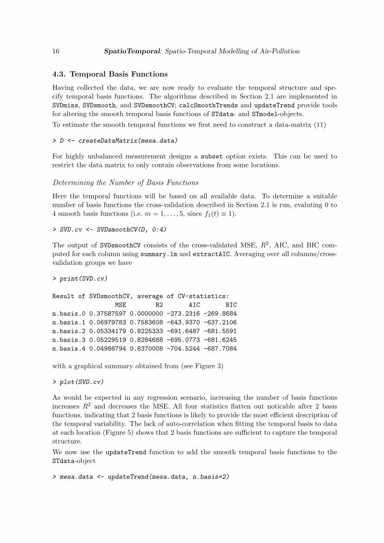
16 SpatioTemporal: Spatio-Temporal Modelling of Air-Pollution

4.3. Temporal Basis Functions

Having collected the data, we are now ready to evaluate the temporal structure and spe-cify temporal basis functions. The algorithms described in Section 2.1 are implemented inSVDmiss, SVDsmooth, and SVDsmoothCV; calcSmoothTrends and updateTrend provide toolsfor altering the smooth temporal basis functions of STdata- and STmodel-objects.

To estimate the smooth temporal functions we first need to construct a data-matrix (11)

> D <- createDataMatrix(mesa.data)

For highly unbalanced measurement designs a subset option exists. This can be used torestrict the data matrix to only contain observations from some locations.

Determining the Number of Basis Functions

Here the temporal functions will be based on all available data. To determine a suitablenumber of basis functions the cross-validation described in Section 2.1 is run, evaluting 0 to4 smooth basis functions (i.e. m = 1, . . . , 5, since f1(t) ≡ 1).

> SVD.cv <- SVDsmoothCV(D, 0:4)

The output of SVDsmoothCV consists of the cross-validated MSE, R2, AIC, and BIC com-puted for each column using summary.lm and extractAIC. Averaging over all columns/cross-validation groups we have

> print(SVD.cv)

Result of SVDsmoothCV, average of CV-statistics:

MSE R2 AIC BIC

n.basis.0 0.37587597 0.0000000 -273.2316 -269.8684

n.basis.1 0.06979783 0.7583608 -643.9370 -637.2106

n.basis.2 0.05334179 0.8225333 -691.6487 -681.5591

n.basis.3 0.05229519 0.8284688 -695.0773 -681.6245

n.basis.4 0.04988794 0.8370008 -704.5244 -687.7084

with a graphical summary obtained from (see Figure 3)

> plot(SVD.cv)

As would be expected in any regression scenario, increasing the number of basis functionsincreases R2 and decreases the MSE. All four statistics flatten out noticable after 2 basisfunctions, indicating that 2 basis functions is likely to provide the most efficient description ofthe temporal variability. The lack of auto-correlation when fitting the temporal basis to dataat each location (Figure 5) shows that 2 basis functions are sufficient to capture the temporalstructure.

We now use the updateTrend function to add the smooth temporal basis functions to theSTdata-object

> mesa.data <- updateTrend(mesa.data, n.basis=2)

Johan Lindstrom, Adam Szpiro, Paul D. Sampson, Silas Bergen, Lianne Sheppard 17

0 1 2 3 4

0.05

0.20

0.35

n.basis

MS

E

0 1 2 3 4

0.0

0.4

0.8

n.basis

R2

0 1 2 3 4

−70

0−

500

−30

0

n.basis

AIC

0 1 2 3 4−

700

−50

0−

300

n.basis

BIC

Figure 3: Cross-validation results for different numbers of smooth temporal trends

Alternatively calcSmoothTrends can be used to compute both the basis functions based onall data and those obtained when excluding each column in the data-matrix

> smooth.trend <- calcSmoothTrends(mesa.data, n.basis=2, cv=TRUE)

This allows for a sensitivity analysis of the temporal basis functions. Here we illustrate this bythe fit at one location (Figure 4), but the different temporal basis functions could be carriedthrough the entire analysis.

> mesa.data.cv <- vector("list", length(smooth.trend$trend.fnc.cv))

> for(i in 1:length(mesa.data.cv)){

+ suppressMessages(mesa.data.cv[[i]] <- updateTrend(mesa.data,

+ fnc=smooth.trend$trend.fnc.cv[[i]]))

+ }

> plot(mesa.data, main="Possible temporal trends",

+ xlab="", ylab="NOx (log ppb)", pch=c(19,NA), cex=.25)

> for(i in 1:length(mesa.data.cv)){

+ plot(mesa.data.cv[[i]], add=TRUE, col=i, pch=NA, lty=c(NA,2))

+ }

Evaluating the Basis Functions

The plot.STdata function can now be used to evaluate how well the temporal basis functionscapture the temporal structure, see Figure 5. plot.STdata fits a linear regression of observa-tions for a particular location of the smooth basis functions, and plots fitted values, residuals,auto-correlation, or partial auto-correlation functions. Here the two temporal basis func-

18 SpatioTemporal: Spatio-Temporal Modelling of Air-Pollution

2000 2002 2004 2006 2008 2010

3.0

4.0

Possible temporal trendsN

Ox

(log

ppb)

●

●

●

●

●●

●

●

●

●

●

●

●

●

●

●

●

●

●

●●

●●

●

●

●

●

●

●

●

●

●●

●

●

●

●

●

●

●

●●

●

●

●

●

●

●

●

●

●

●

●

●

●

●●

●

●

●

●

●

●

●

●

●●

●

●

●

●

●

●

●

●

●

●

●●

●

●

●

●

●

●●

●

●

●

●

●

●

●

●

●

●

●●

●

●

●

●

●

●

●

●

●

●●

●●

●

●●

●

●●

●●

●

●

●

●

●

●●

●

●

●

●

●

●

●

●

●

●

●

●

●

●

●

●

●

●

●

●

●

●

●

●

●

●●

●

●

●

●

●

●

●

●

●

●

●

●

●

●

●

●●

●

●

●

●

●

●

●

●●

●

●

●

●

●

●

●

●

●

●

●

●

●

●

●

●

●

●

●

●

●

●

●

●

●

●

●

●

●

●

●

●

●

●

●●

●

●

●

●

●

●

●

●●●

●●

●

●

●

●

●

●

●

●

●

●

●●

●●

●

●

●

●

●●

●

●

●

●

●

●

●

●

●

●

●

●

●

●

●

●

●

●

●●

●

●

●●

●

●

●

●

●

●

●

Figure 4: Cross-validated temporal basis functions. The solid line is the regression fit of 2basis functions, based on all data, to observations at AQS site 60370002, the dashed lines arethe corresponding fits of basis functions obtained when excluding one column at a time fromthe data-matrix.

tions capture the temporal variability in the data, as illustrated by residuals and correlationfunctions.

> par(mar=c(3.3,3.3,1.5,1), mgp=c(2,1,0))

> layout(matrix(c(1,1,2,2,3,4), 3, 2, byrow=TRUE))

> plot(mesa.data, "obs", ID="60370113",

+ xlab="", ylab="NOx (log ppb)",

+ main="Temporal trend 60370113")

> plot(mesa.data, "res", ID="60370113",

+ xlab="", ylab="NOx (log ppb)")

> plot(mesa.data, "acf", ID="60370113")

> plot(mesa.data, "pacf", ID="60370113")

Deterministic Basis Functions

In lieu of the SVD based basis functions we could use a set of deterministic temporal functions,e.g. f1(t) = 1, f2(t) = 2πt/365, f3(t) = sin(2πt/365), and f4(t) = cos(2πt/365). Specifyingthese and comparing to the data driven smooths extrated above (see Figure 6) we note that,for this data, three deterministic basis functions achieve a slightly worse fit than the twofunctions based on smoothed SVDs.

> mesa.data.fnc <- updateTrend(mesa.data, fnc=function(x){

+ x = 2*pi*as.numeric(x)/365;

+ return( cbind(x, sin(x), cos(x)) )})

> par(mfrow=c(2,1), mar=c(2.3,3.3,1.5,1), mgp=c(2,1,0))

> for(i in c("60370016","60371103")){

+ plot(mesa.data, ID=i, pch=c(19,NA), cex=.25, xlab="",

+ ylab="NOx (log ppb)", main=paste("AQS site",i))

+ plot(mesa.data.fnc, ID=i, add=TRUE, col=2, pch=NA)

+ }

Johan Lindstrom, Adam Szpiro, Paul D. Sampson, Silas Bergen, Lianne Sheppard 19

2000 2002 2004 2006 2008 2010

2.0

3.0

4.0

5.0

Temporal trend 60370113

NO

x (lo

g pp

b)●

●●

●

●●

●

●

●●●●

●●

●

●●●●

●●●●●●●●

●

●●●●●●●●

●●

●

●●

●●

●●

●

●●●

●

●

●

●●●●

●●

●

●●

●●

●●

●●●

●

●

●●●●

●

●

●●●

●

●●

●●

●●●●●●

●●●

●●

●●●

●

●

●●

●

●●●●

●

●

●●●

●●

●

●●

●

●

●●●●●

●

●●●●

●●●●

●

●

●●●●

●

●

●

●

●

●●●

●●

●

●●

●●●●

●

●

●

●●●●

●

●●●

●

●

●

●

●●

●●

●●●

●●●●

●●●●●

●

●

●

●●

●●●

●●

●●

●●

●●

●●●

●●●●●●

●●

●

●●●

●

●●●●

●

●●●●

●

●

●●

●●

●

●

●

●●●

●

●

●

●●●

●●●●

●●

●●

●

●

●

●●●●●

●

●

●●

●●●

●●●●

●●●

●

●

●

2000 2002 2004 2006 2008 2010

−0.

50.

00.

5

Residuals 60370113

NO

x (lo

g pp

b)

●

●●

●

●

●

●

●

●

●

●

●

●

●

●

●●●

●

●●

●

●

●

●

●

●

●●●

●●●●●●

●●

●

●●

●

●

●●

●

●

●

●

●

●

●

●●●

●●

●

●

●

●

●●

●

●

●

●●

●

●

●●●

●

●

●

●

●●

●

●●

●●

●

●●●

●●

●●

●

●

●

●●●

●

●

●

●

●

●

●

●

●

●

●

●

●●

●●

●

●●

●

●

●

●

●

●●

●

●

●●●

●

●

●●

●

●

●

●●

●

●

●

●

●

●

●

●

●

●

●

●

●●

●●●●

●

●

●

●

●●●

●

●

●●

●

●

●

●

●

●

●

●

●

●

●

●●●

●

●

●

●●

●

●

●

●

●

●

●●●

●

●

●●

●

●

●

●

●●●

●●

●

●

●●

●

●

●

●

●●

●

●

●●

●

●

●

●●

●

●

●

●●

●

●

●

●

●

●

●●

●

●

●

●●

●

●

●●●●●

●●

●

●

●

●●●

●●

●

●

●

●

●

●●

●●●●

●●

●

●

●

●

0 5 10 15 20

0.0

0.4

0.8

Lag

AC

F

ACF for 60370113

5 10 15 20

−0.

100.

000.

10

Lag

Par

tial A

CF

PACF for 60370113

Figure 5: The smooth temporal trends fitted to data at site 60370113. Fitted trends, residuals,auto-correlation, and partial auto-correlation functions are shown.

2000 2002 2004 2006 2008 2010

2.5

3.5

AQS site 60370016

NO

x (lo

g pp

b)

●

●

●

●

●

●

●

●

●

●

●

●●●

●

●

●

●

●

●●

●●

●

●

●

●

●●

●●

●

●

●

●●

●

●

●●

●

●●

●●●

●

●●

●

●

●

●

●

●

●●

●

●●

●●

●

●

●

●●

●

●

●

●●

●●

●

●●

●●

●

●

●

●

●

●

●

●●

●●

●

●

●

●

●

●

●

●

●

●

●

●

●

●

●●

●

●●

●

●

●

●

●●

●

●●

●

●●

●

●

●●

●●

●

●

●

●

●

●

●

●

●

●●

●

●

●

●●

●

●

●

●

●●

●

●

●

●●●

●

●

●

●

●

●

●

●

●●

●

●

●

●

●

●●

●●

●

●

●

●●

●

●

●

●●

●

●

●

●

●

●

●

●

●●

●●

●

●

●

●

●

●

●

●

●

●

●

●

●●

●●

●

●

●●●

●

●●

●

●

●●

●●

●

●●

●

●●

●●●

●

●

●

●

●●

●

●

●●

●

●●

●●●

●●

●

●

●

●

●●

●

●

●

●

●

●

●

●

●●

●●

●

●

●●

●

●

●●

●

2000 2002 2004 2006 2008 2010

3.0

5.0

AQS site 60371103

NO

x (lo

g pp

b)

●

●

●

●

●●

●

●

●

●

●

●●

●

●

●

●

●

●

●

●

●●

●

●

●●

●●

●●

●●●●●

●

●

●

●

●●●

●●

●

●●

●

●

●

●

●●

●

●

●

●

●

●●

●●

●

●

●●

●

●

●

●

●

●

●

●

●

●●●

●

●

●

●

●

●

●

●

●●●

●

●

●

●

●

●

●●

●

●

●

●

●

●

●

●

●

●

●

●●

●●

●●

●

●

●

●

●●

●●

●

●

●

●

●

●

●●

●●●

●●●

●

●

●

●●

●

●

●

●●

●●

●●

●●

●

●

●

●

●

●●●●

●

●●

●

●

●

●

●

●

●

●

●

●

●

●

●

●●

●●

●●

●

●

●

●

●

●

●

●●●

●

●

●

●

●

●

●

●

●

●●

●

●●●●

●

●●

●

●●●

●

●

●●●●

●●

●●

●

●

●

●●

●

●

●

●

●

●●

●

●

●

●

●

●

●●

●●

●

●●

●

●

●

●●●

●

●

●

●

●●

●●●

●

●●

●

●

●

●

●

●

●

Figure 6: Comparing the fit of 2 smooth (black) and 3 deterministic (red) basis functions attwo locations.

4.4. Specifying the Model

Having constructed a STdata-object with suitable temporal basis functions we are now readyto create a STmodel-object that can be used by the estimation and prediction functions of

20 SpatioTemporal: Spatio-Temporal Modelling of Air-Pollution

SpatioTemporal. A STmodel-object is created through createSTmodel, by adding covarianceand covariate specifications for the β- and ν-fields to a STdata-object.

Suitable covariates and covariance structures for the β-fields in (3) can be determined byconsidering the empirical estimates of these fields obtained by regressing the observationsat each location on the temporal basis functions. The resulting regression coefficients canbe analysed using standard geo-statistical software, e.g. provided by the R-packages geoR(Ribeiro and Diggle 2001) or fields (Furrer et al. 2012), to determine suitable mean andcovariance models (see also Mercer et al. 2011).

Here we briefly illustrate the point by computing the regression coefficents and comparingthem to a few possible covariates (Figure 7).

> beta.lm <- estimateBetaFields(mesa.data)

> par(mfrow=c(1,2), mar=c(3.3,2.3,1.5,1), mgp=c(2,1,0))

> plotCI(mesa.data$covars$log10.m.to.a1, beta.lm$beta[,1],

+ uiw=1.96*beta.lm$beta.sd[,1], ylab="", xlab="Distance to A1-road",

+ main="Beta-field for f1(t)")

> plotCI(mesa.data$covars$km.to.coast, beta.lm$beta[,2],

+ uiw=1.96*beta.lm$beta.sd[,2], ylab="", xlab="Distance to coast",

+ main="Beta-field for f2(t)")

To simplify the analysis of unbalanced measurement designs estimateBetaFields providesa subset option that restricts the evaluated locations.

2.0 2.5 3.0 3.5

3.0

3.5

4.0

Beta−field for f1(t)

Distance to A1−road

●

●

●

●

●

● ●

●

●●

●

●

●●

●

●

●●

●

●

●

●

●

●

●

2 4 6 8 10 14

−1.

0−

0.6

−0.

2

Beta−field for f2(t)

Distance to coast

●

●

●

●

●●●●●●●

●●

●

●●

●●

●

●●

●

●

●

●

Figure 7: Regression estimates of β1(s) and β2(s) at each location, with 95% confidenceintervals, as a function of the distance to A1 roads or the distance to coast.

Partially based on Figure 7 we specify different mean models for the three β-fields, butuse an exponential covariance function without nugget for all fields; it is possible to specifydifferent covariance functions for each β-field. Possible covariance functions are describe bythe functions namesCovFuns and parsCovFuns, while updateCovf can be used to alter thecovariance structure of an existing STmodel.

> LUR <- list(~log10.m.to.a1+s2000.pop.div.10000+km.to.coast,

Johan Lindstrom, Adam Szpiro, Paul D. Sampson, Silas Bergen, Lianne Sheppard 21

+ ~km.to.coast, ~km.to.coast)

> cov.beta <- list(covf="exp", nugget=FALSE)

For the ν-field we use an exponential covariance with a nugget that can differ between AQSand MESA fixed sites.

> cov.nu <- list(covf="exp", nugget=~type, random.effect=FALSE)

In this specification the log-nugget will be given by a linear model

log σ2nugget(s) = θν,const + θν,type1(s ∈ MESA fixed sites). (36)

The random.effect=FALSE option specifies that we do not want a random mean for eachν(·, t) field. A random effect in time provides a way of capturing temporally uncorrelatedlarge scale deviations from the smooth temporal basis functions. Using both a regressionmodel for log-nugget (36) and a temporal random effect the full spatio-temporal covariancefor the ν-field would be

rν(s1, t1; s2, t2) =

σ2

nugget(s1) + g(0) + τ2, if s1 = s2, t1 = t2,

g(s1 − s2) + τ2, if s1 6= s2, t1 = t2,

0, if t1 6= t2,

(37)

where σ2nugget(s) is a (spatially varying) nugget, g(s) is a stationary covariance function, and

τ2 is the variance of a temporal random effect.

The final step is to specify coordinates for the observations and create the STmodel-object:

> locations <- list(coords=c("x","y"), long.lat=c("long","lat"),

+ others="type")

> mesa.model <- createSTmodel(mesa.data, LUR=LUR, ST="lax.conc.1500",

+ cov.beta=cov.beta, cov.nu=cov.nu,

+ locations=locations)

In locations the element coords specifies which components of mesa.data$covars to usewhen computing distances between observation locations; the elements long.lat and others

give additional fields that are carried over from mesa.data$covars to mesa.model$locations,e.g. data that could be useful for plotting. All variables referenced in the LUR and cov.nu$nugget

formulas, and in the locations-list must be found in mesa.data$covars.

Most of the S3-methods available for STdata-objects also exists for STmodel-objects.

4.5. Parameter Estimation and Prediciton

Parameters of the spatio-temporal model (10) can by obtained by maximising (16) throughestimate.STmodel. Given (estimated) parameters predictions are obtained from predict.STmodel.

Estimation

To avoid potential numerical optimisation issues, the estimation function allows for multiplestarting points, returning all optima found. The functions loglikeSTdim and loglikeSTnames

gives the number of parameters (and other model dimension) and the names, i.e. expectedorder, of the parameters. Using this information a two column matrix, where each columnrepresents a different optimisation starting point, is constructed

22 SpatioTemporal: Spatio-Temporal Modelling of Air-Pollution

> dim <- loglikeSTdim(mesa.model)

> x.init <- cbind(c( rep(2, dim$nparam.cov-1), 0),

+ c( rep(c(1,-3), dim$m+1), -3, 0))

> rownames(x.init) <- loglikeSTnames(mesa.model, all=FALSE)

Model parameters are then estimated through

> est.mesa.model <- estimate(mesa.model, x.init, type="p", hessian.all=TRUE)

where type allows us to use either the f(ull), p(rofile) (16), or r(eml) (17) log-likelihoods.Since the estimation takes time (10–15 minutes, depending on the computer) the packagecontains precomputed results which we load and examine.

> data(est.mesa.model, package="SpatioTemporal")

> print(est.mesa.model)

Optimisation for STmodel with 2 starting points.

Results: 2 converged, 0 not converged, 0 failed.

Best result for starting point 1, optimisation has converged

No fixed parameters.

Estimated parameters for all starting point(s):

[,1] [,2]

gamma.lax.conc.1500 0.0008975546 0.0009008652

alpha.const.(Intercept) 3.7402698246 3.7406058853

alpha.const.log10.m.to.a1 -0.2021288763 -0.2022633497

alpha.const.s2000.pop.div.10000 0.0402182221 0.0401923686

alpha.const.km.to.coast 0.0374363255 0.0374629689

alpha.V1.(Intercept) -0.7429226257 -0.7411611359

alpha.V1.km.to.coast 0.0174017754 0.0172645957

alpha.V2.(Intercept) -0.1292573245 -0.1281826343

alpha.V2.km.to.coast 0.0155467684 0.0154883000

log.range.const.exp 2.4245453422 2.4205527321

log.sill.const.exp -2.7522202309 -2.7568455241

log.range.V1.exp 2.9175969067 2.9484089871

log.sill.V1.exp -3.5231738064 -3.5086290882

log.range.V2.exp 1.7816565861 1.8062154010

log.sill.V2.exp -4.6812486307 -4.6730245593

nu.log.range.exp 4.3836003026 4.3839197279

nu.log.sill.exp -3.2126038230 -3.2123312163

nu.log.nugget.(Intercept).exp -4.4121007058 -4.4118479775

nu.log.nugget.typeFIXED.exp 0.6766505805 0.6748262774

Function value(s):

[1] 5748.563 5748.561

Johan Lindstrom, Adam Szpiro, Paul D. Sampson, Silas Bergen, Lianne Sheppard 23

The estimation results indicate that the optimisation for both starting points have converged,starting point 1 being marginally better, with very similar parameter estimates and functionvalues.

Plots of the estimated parameters together with approximate 95%-confidence intervals com-puted using the Hessian, i.e. the observed information matrix (Casella and Berger 2002,Ch. 10), can be seen in Figure 10 below; this Figure also includes parameter estimates fromthe cross-validation. Confidence intervals for covariance parameters of the residual ν-field aremuch smaller than the corresponding intervals for the covariance parameters characterisingthe β-fields. This is due to us having only one replicate of each β-field — in principal givenby the regression of observations on the smooth temporal basis functions — but T = 280replicates of the residual ν-field, one for each timepoint — in principal given by the residualsfrom the regression.

Predictions

Given estimated parameters, predictions can be computed for the Gaussian model using (23);for log-Gaussian processes using (27) or (29); and for the temporal averages using (26a) or(32).

> pred <- predict(mesa.model, est.mesa.model, LTA=TRUE, type="p")

> pred.log <- predict(mesa.model, est.mesa.model, LTA=TRUE,

+ transform="unbiased", type="p")

Here the type option controls the computation of variances, with type="p" (or type="f")the regression parameters are assumed known resulting in variances/MSPEs according to (24)or (28); for type="r" regression parameters are assumed unknown and variances/MSPEs aregiven by (25) or (31). Items computed include predictions of y(s, t), contributions to thepredictions from different parts of the model (see Figure 1 above), prediction variances (orMSPE), and predictions of the β-fields; print.predictSTmodel can be used to display allcomputed components.

The latent β-fields (20) can be compared to the empirical, regression based, estimates presen-ted in Figure 7. Comparing these two estimates (see Figure 8) we see that they are close, withthe largest discrepancies occuring for β’s associated with the second temporal trend, f3(t).However, the uncertainty for these β’s are substantial.

> par(mfrow=c(2,2), mar=c(3.3,3.3,1.5,1), mgp=c(2,1,0), pty="s")

> for(i in 1:3){

+ plotCI(x=beta.lm$beta[,i], y=pred$beta$EX[,i],

+ uiw=1.96*beta.lm$beta.sd[,i], err="x",

+ pch=NA, sfrac=0.005,

+ main=paste("Beta-field for f", i, "(t)", sep=""),

+ xlab="Empirical estimate",

+ ylab="Spatio-Temporal Model")

+ plotCI(x=beta.lm$beta[,i], y=pred$beta$EX[,i],

+ uiw=1.96*sqrt(pred$beta$VX[,i]),

+ add=TRUE, pch=NA, sfrac=0.005)

+ abline(0, 1, col="grey")

+ }

24 SpatioTemporal: Spatio-Temporal Modelling of Air-Pollution

3.0 3.5 4.0

3.0

3.4

3.8

4.2

Beta−field for f1(t)

Empirical estimate

Spa

tio−

Tem

pora

l Mod

el

−1.0 −0.8 −0.6 −0.4 −0.2

−0.

8−

0.6

−0.

4−

0.2

Beta−field for f2(t)

Empirical estimate

Spa

tio−

Tem

pora

l Mod

el

−0.4 −0.2 0.0 0.2

−0.

20.

00.

10.

2

Beta−field for f3(t)

Empirical estimate

Spa

tio−

Tem

pora

l Mod

el

Figure 8: Comparison of the regression based and full (20) estimates of the β–field, includingthe uncertainties in both estimates.

The predictions also include the temporal averages at each location. In Figure 9 these predic-tions are compared to the temporal averages of observations at each site. A minor issue (seealso Section 2.4) with this comparison is the temporal miss-match between predictions (aver-aged over 10-years) and the observations (averaged over 1 to 10 years depending on availabledata).

> par(mfrow=c(1,2), mar=c(3.3,3.3,1.5,1), mgp=c(2,1,0))

> with(pred$LTA, plotCI(colMeans(D, na.rm=TRUE), EX, uiw=1.96*sqrt(VX.pred),

+ xlim=c(2.9,4.4), ylim=c(2.9,4.4),

+ ylab="Predictions", xlab="Observations",

+ main="Average NOx (log ppb)"))

> abline(0, 1, col="grey")

> with(pred.log$LTA, plotCI(colMeans(exp(D), na.rm=TRUE),

+ EX, uiw=1.96*sqrt(VX.pred),

+ xlim=c(25,95), ylim=c(25,95),

+ ylab="Predictions", xlab="Observations",

+ main="Average NOx (ppb)"))

Johan Lindstrom, Adam Szpiro, Paul D. Sampson, Silas Bergen, Lianne Sheppard 25

> abline(0, 1, col="grey")

3.0 3.5 4.0

3.0

3.5

4.0

Average NOx (log ppb)

Observations

Pre

dict

ions

●

●

●

●

●

●●

●

●

●●

●

●●

●

●

●●

●

●

●

●

●

●

●

30 50 70 90

3050

7090

Average NOx (ppb)

ObservationsP

redi

ctio

ns

●

●

●

●

●

●●

●

●

●

●●

●

●●

●

●●

●

●

●

●

●

●

●

Figure 9: Observed and predicted temporal averages at each location, both for the Gaussian(left) and log-Gaussian (right) processes. The difference between observed and predictedvalues is (partially) due to temporally incomplete observations, i.e. the predicted average isover the entire 10-year period, regardless of when we have observations.

4.6. Cross-validation and Model Evaluation

The model’s predictive ability can be evaluated through cross-validataion (Lindstrom et al.2013). The first step is to define a vector that splits the observations into CV-groups

> Ind.cv <- createCV(mesa.model, groups=10, min.dist=.1)

For the ith CV-group observations for which Ind.cv = i are predicted using parameter es-timates and conditional expectations based on the observations where Ind.cv 6= i. Since theprimary focus when constructing the package was spatial prediction the number of locationsin each group will be roughly even

> ID.cv <- sapply(split(mesa.model$obs$ID, Ind.cv), unique)

> print( sapply(ID.cv, length) )

1 2 3 4 5 6 7 8 9 10

3 3 3 2 2 2 2 2 2 4

although the number of observations in each grup may differ substantially

> table(Ind.cv)

Ind.cv

1 2 3 4 5 6 7 8 9 10

438 389 811 556 546 165 228 487 160 797

26 SpatioTemporal: Spatio-Temporal Modelling of Air-Pollution

Having four locations in the 10th group is due to the fact that AQS site 60371103 is colocatedwith MESA Air site L001.

> print(mesa.model$D.beta[ID.cv[[10]],ID.cv[[10]]])

60371103 60371601 60371701 L001

60371103 0.00000000 16.36527 43.75141 0.08363892

60371601 16.36527030 0.00000 29.06447 16.44669372

60371701 43.75141252 29.06447 0.00000 43.83429713

L001 0.08363892 16.44669 43.83430 0.00000000

As seen from the distance matrix above, the two stations are only 0.084 km apart (less thanmin.dist=.1) causing createCV to treat them as “one” location.

For cases where the primary interest is in temporal predictions suitable Ind.cv vectors couldbe construted with the help of elements in mesa.model$obs.

Estimation and Prediciton

For the estimation part of the cross-validation a set of starting point(s) is needed; here weuse the optimum found in the optimisation and the starting point, of the two possible, whichlead to the optimum.

> x.init <- coef(est.mesa.model, pars="cov")[,c("par","init")]

As before the estimation is computationally expensive

> est.cv.mesa <- estimateCV(mesa.model, x.init, Ind.cv)

and we load precomputed results.

> data(est.cv.mesa, package="SpatioTemporal")

Studying results from print(est.cv.mesa) (not shown) it can be seen that all 10 of the estim-ations have converged, and comparing these estimates (available through coef(est.cv.mesa))to those obtained for the entire data set shows reasonable agrement, both with regards tovalues and uncertainties (Figure 10).

> par(mfrow=c(1,1), mar=c(13.5,2.5,.5,.5), las=2)

> with(coef(est.mesa.model, pars="all"),

+ plotCI((1:length(par))+.3, par, uiw=1.96*sd,

+ col=2, xlab="", xaxt="n", ylab=""))

> boxplot(est.cv.mesa, "all", boxwex=.4, col="grey", add=TRUE)

Given parameter estimates the prediction part of the cross-validation can be carried out foreither Gaussian or log-Gaussian models. In both cases temporal averages are computed basedon only the observed time-points, as in (35).

Johan Lindstrom, Adam Szpiro, Paul D. Sampson, Silas Bergen, Lianne Sheppard 27

−4

−2

0

2

4

●

●

●● ●

●

● ● ●

●

●

●

●

●

●

●

●

●

●

●●● ● ●●●●●

●

●

●

●

gam

ma.

lax.

conc

.150

0

alph

a.co

nst.(

Inte

rcep

t)

alph

a.co

nst.l

og10

.m.to

.a1

alph

a.co

nst.s

2000

.pop

.div

.100

00

alph

a.co

nst.k

m.to

.coa

st

alph

a.V

1.(I

nter

cept

)

alph

a.V

1.km

.to.c

oast

alph

a.V

2.(I

nter

cept

)

alph

a.V

2.km

.to.c

oast

log.

rang

e.co

nst.e

xp

log.

sill.

cons

t.exp

log.

rang

e.V

1.ex

p

log.

sill.

V1.

exp

log.

rang

e.V

2.ex

p

log.

sill.

V2.

exp

nu.lo

g.ra

nge.

exp

nu.lo

g.si

ll.ex

p

nu.lo

g.nu

gget

.(In

terc

ept)

.exp

nu.lo

g.nu

gget

.type

FIX

ED

.exp

−4

−2

0

2

4

Figure 10: Estimated parameters and approximate 95% confidence intervals (red) comparedto parameter estimates from 10-fold cross-validation (box-plots).

> ##pred.cv.mesa <- predictCV(mesa.model, est.cv.mesa, LTA=TRUE)

> data(pred.cv.mesa, package="SpatioTemporal")

> pred.cv.mesa.log <- predictCV(mesa.model, est.cv.mesa,

+ LTA=TRUE, transform="unbiased")

As for estimateCV the computations take time and precomputed results are included indata(CV.mesa.model) which we loaded previously.

Alternatively the function computeLTA can be applied to the result from predictCV, howeverthis will only compute the temporal averages in (35) and will not include the variances from(26b) or (33a)-(33c).

Model Evaluation

The summary.predCVSTmodel function computes RMSE, R2, and coverage of prediction in-tervals for the cross-validation. For the log-Gaussian data we have:

> summary(pred.cv.mesa.log)

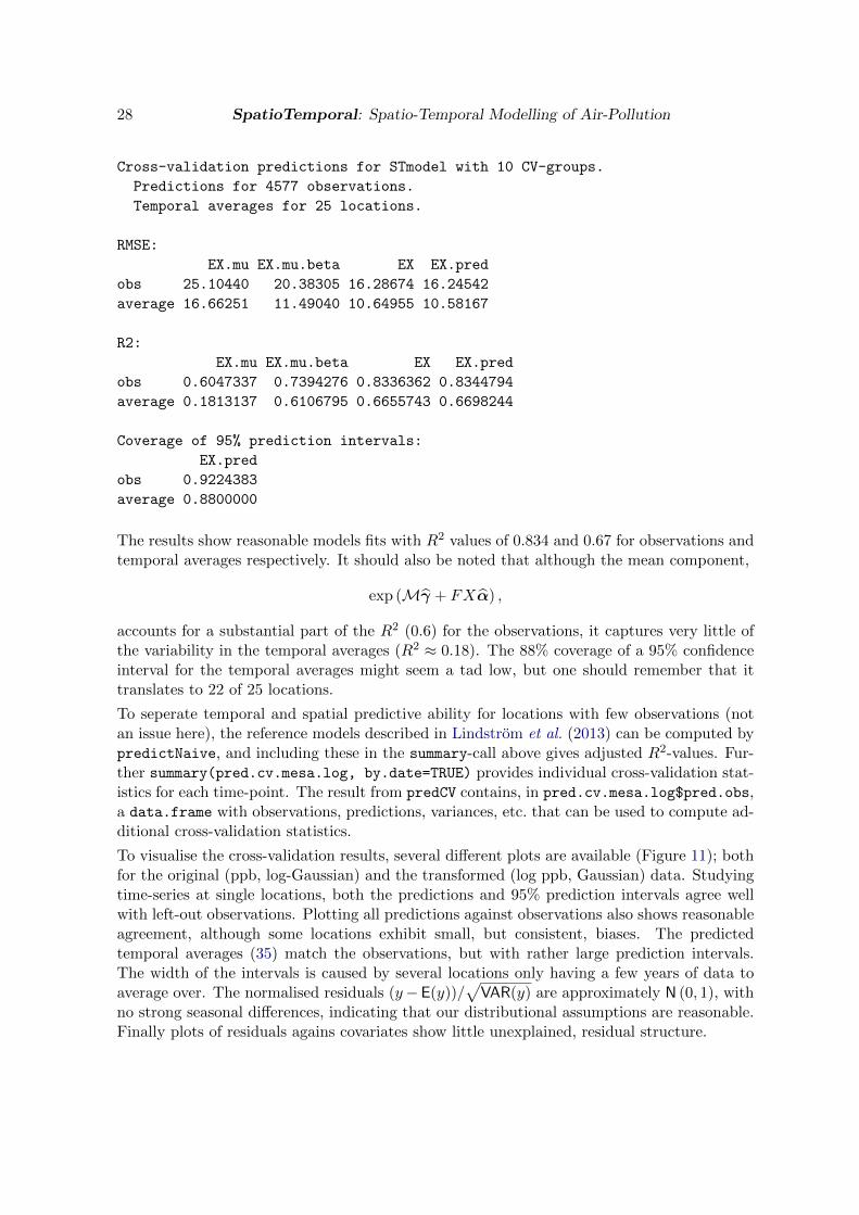
28 SpatioTemporal: Spatio-Temporal Modelling of Air-Pollution

Cross-validation predictions for STmodel with 10 CV-groups.

Predictions for 4577 observations.

Temporal averages for 25 locations.

RMSE:

EX.mu EX.mu.beta EX EX.pred

obs 25.10440 20.38305 16.28674 16.24542

average 16.66251 11.49040 10.64955 10.58167

R2:

EX.mu EX.mu.beta EX EX.pred

obs 0.6047337 0.7394276 0.8336362 0.8344794

average 0.1813137 0.6106795 0.6655743 0.6698244

Coverage of 95% prediction intervals:

EX.pred

obs 0.9224383

average 0.8800000

The results show reasonable models fits with R2 values of 0.834 and 0.67 for observations andtemporal averages respectively. It should also be noted that although the mean component,

exp (Mγ + FXα) ,

accounts for a substantial part of the R2 (0.6) for the observations, it captures very little ofthe variability in the temporal averages (R2 ≈ 0.18). The 88% coverage of a 95% confidenceinterval for the temporal averages might seem a tad low, but one should remember that ittranslates to 22 of 25 locations.

To seperate temporal and spatial predictive ability for locations with few observations (notan issue here), the reference models described in Lindstrom et al. (2013) can be computed bypredictNaive, and including these in the summary-call above gives adjusted R2-values. Fur-ther summary(pred.cv.mesa.log, by.date=TRUE) provides individual cross-validation stat-istics for each time-point. The result from predCV contains, in pred.cv.mesa.log$pred.obs,a data.frame with observations, predictions, variances, etc. that can be used to compute ad-ditional cross-validation statistics.

To visualise the cross-validation results, several different plots are available (Figure 11); bothfor the original (ppb, log-Gaussian) and the transformed (log ppb, Gaussian) data. Studyingtime-series at single locations, both the predictions and 95% prediction intervals agree wellwith left-out observations. Plotting all predictions against observations also shows reasonableagreement, although some locations exhibit small, but consistent, biases. The predictedtemporal averages (35) match the observations, but with rather large prediction intervals.The width of the intervals is caused by several locations only having a few years of data toaverage over. The normalised residuals (y−E(y))/

√VAR(y) are approximately N (0, 1), with

no strong seasonal differences, indicating that our distributional assumptions are reasonable.Finally plots of residuals agains covariates show little unexplained, residual structure.

Johan Lindstrom, Adam Szpiro, Paul D. Sampson, Silas Bergen, Lianne Sheppard 29

> par(mar=c(3.3,3.3,1.5,1), mgp=c(2,1,0))

> layout(matrix(c(1,1,2,2,3,4,5,6), 4, 2, byrow=TRUE))

> plot(pred.cv.mesa, ID="60371601", xlab="", ylab="NOx (log ppb)",

+ main="Predictions for 60371601", lty=c(1,NA), lwd=2,

+ pch=c(NA,19), cex=.75)

> plot(pred.cv.mesa, ID="60371601", pred.type="EX.mu",

+ lty=4, lwd=2, col="blue", add=TRUE)

> plot(pred.cv.mesa, ID="60371601", pred.type="EX.mu.beta",

+ lty=2, lwd=2, col="green", add=TRUE)

> plot(pred.cv.mesa.log, ID="60371601", xlab="", ylab="NOx (ppb)",

+ main="Predictions for 60371601", pred.type="EX.pred",

+ lty=c(1,NA), lwd=2, pch=c(NA,19), cex=.75)

> plot(pred.cv.mesa.log, ID="60371601", pred.type="EX.mu",

+ lty=4, lwd=2, col="blue", add=TRUE)

> plot(pred.cv.mesa.log, ID="60371601", pred.type="EX.mu.beta",

+ lty=2, lwd=2, col="green", add=TRUE)

> legend("topright", c("Observations", "Predictions",

+ "Contribution from beta",

+ "Contribution from mean",

+ "95% CI"), bty="n",

+ lty=c(NA,1,2,4,NA), lwd=c(NA,2,2,2,NA),

+ pch=c(19,NA,NA,NA,15), pt.cex=c(.75,NA,NA,NA,2.5),

+ col=c("red", "black", "green", "blue", "grey"))

> plot(pred.cv.mesa, "obs", ID="all", pch=c(19,NA), cex=.25, lty=c(NA,2),

+ col=c("ID", "black", "grey"), xlab="Observations",

+ ylab="Predictions", main="Cross-validation NOx (log ppb)")

> with(pred.cv.mesa.log$pred.LTA, plotCI(obs, EX.pred, uiw=1.96*sqrt(VX.pred),

+ xlab="Observations", ylab="Predictions",

+ main="Temporal average NOx (ppb)"))

> abline(0, 1, col="grey")

> I.season <- as.factor(as.POSIXlt(pred.cv.mesa$pred.obs$date)$mon+1)

> levels(I.season) <- c(rep("Winter",2), rep("Spring",3),

+ rep("Summer",3), rep("Fall",3), "Winter")

> qqnorm(pred.cv.mesa, norm=TRUE, main="Normalised residuals",

+ col=I.season)

> legend("bottomright", legend=as.character(levels(I.season)),

+ pch=1, col=1:nlevels(I.season), bty="n")

> scatterPlot(pred.cv.mesa, STdata=mesa.model, covar="log10.m.to.a1",

+ group=I.season, col=c(2:5,1), type="res",

+ xlab="Distance to A1-Road", ylab="Residuals",

+ main="Residuals (log ppb)")

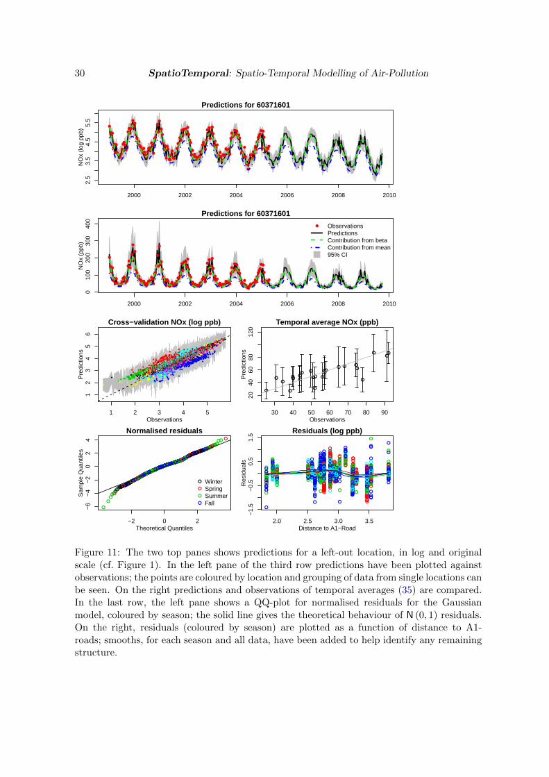
30 SpatioTemporal: Spatio-Temporal Modelling of Air-Pollution

2000 2002 2004 2006 2008 2010

2.5

3.5

4.5

5.5

Predictions for 60371601

NO

x (lo

g pp

b)

●

●

●

●

●

●

●

●

●

●

●

●

●●●

●●

●

●

●

●

●

●

●

●

●●

●●

●●●●

●

●●●

●●●●

●●

●

●●

●

●

●

●

●●

●

●

●

●

●

●●

●●

●

●

●●

●●

●

●●

●●

●

●

●●●●

●

●

●●

●

●

●●●●

●●●

●●

●●●

●

●

●

●

●

●

●

●

●

●

●

●●

●●

●

●

●

●●●

●●●●

●

●

●

●●

●

●●

●●●

●

●●

●

●

●

●●

●

●

●●

●

●●

●●

●

●●●

●

●

●

●

●●●●

●

2000 2002 2004 2006 2008 2010

010

020

030

040

0

Predictions for 60371601

NO

x (p

pb)

●

●

●

●

●●

●

●

●●●●●●●●●

●

●

●

●

●

●

●

●

●

●●●

●●●●

●●●●

●●●●

●●

●

●●

●

●

●

●

●●

●

●

●●

●

●●

●●●●●●

●●●●●

●●

●

●

●●●

●

●

●

●●

●●●●●●●●●

●●

●●●●

●

●

●

●

●

●

●

●

●●

●●

●●●●●

●●●●●●●

●

●

●

●●

●

●

●

●●●

●

●●●

●

●●●●

●●●●

●●

●●

●

●●●

●

●

●

●

●●●●●

● ObservationsPredictionsContribution from betaContribution from mean95% CI

1 2 3 4 5

12

34

56

Cross−validation NOx (log ppb)

Observations

Pre

dict

ions

●● ●

●

●

● ●●

●

●

●

●

●

●●

●

●

●

●

●

●

●●

●

●

●

●

●

●

●●

●

●

●●

●

●

●

●

●

●

●

●

●

●

●●

●

●

●

●

●

●

●

●

●

●

●●●●

●

●

●

●●●

●

●

●●●●●

●

●

●●

●

●

●

●

●

●

●●●

●

●●

●

●

●●

●

●

●

●

●

●

●

●

●●

●●

●

●

●

●

●

●

●

●

●

●

●

●

●

●

●

●

●●●●

●

●

●

●

●

●

●

●

●

●●

●

●

●

●

●●

●

●

●

●

●●

●

●

●

●

●

●

●

●

●

●

●

●

●

●

●

●

●

●●●●

●

●

●

●

●

●

●

●

●

●●

●

●●●

●

●

●

●

●

●

●

●

●

●

●

●●●

●

●

●●

●●●

●

●

●

●

●

●

●

●

●

●

●

●

●

●

●●

●●●

●

●

●●

●

●

●

●

●

●

●

●

●

●

●

●

●

●

●

●

●

●●

●

●

●

●●

●

●

●

●

●

●

●●

●

●

●

●

●

●

●

●

●

●

●

●

●

●

●

●●

●

●

●

●

●

●

●

●●

●

●

●

●

●

●

●

●

●

●

●●

●

●

●

●

●

●

●

●

●

●

●●

●

●

●

●

●

●

●

●

●

●●

●

●

●

●●

●

●

●

●

●

●

●

●

●

●

●

●

●

●

●

●

●●

●

●

●

●

●

●

●

●●

●

●

●●

●

●

●

●●

●

●

●●

●

●

●●

●

●

●

●

●●●

●

●●

●

●

●●●

●

●

●

●

●

●

●

●●

●

●

●

●

●

●

●●●

●

●

●

●●●

●●

●

●

●●

●

●

●

●

●

●

●

●●

●

●

●

●

●

●

●

●

●

●

●

●

●

●

●

●

●

●●

●●●●

●

●

●

●

●

●

●

●

●

●

●

●

●

●

●

●

●

●

●

●●

●

●

●

●

●

●

●

●●

●

●

●

●

●

●

●

●

●

●

●

●

●

●

●

●

●

●

●

●

●

●

●

●

●

●

●

●

●

●

●

●●●

●

●●●

●●

●

●●

●

●

●

●●

●

●

●

●

●●

●●

●

●●

●●

●

●●●

●●

●

●●

●●

●

●

●

●

●

●●●

●

●

●

●

●

●

●

●

●

●●●

●

●●

●

●●

●

●

●

●

●

●

●

●

●

●

●●

●

●

●

●

●●

●●

●

●

●

●

●

●

●

●

●

●

●

●

●

●●

●

●

●

●●

●

●

●

●

●

●

●●

●

●

●

●

●

●

●

●

●●

●

●

●●

●●●

●

●

●

●

●

●

●

●

●

●●●

●

●

●●

●

●

●

●

●

●

●

●

●

●

●

●

●

●

●●

●

●

●

●

●●●

●

●

●

●●●

●

●

●

●

●

●

●●

●

●

●

●

●●

●

●

●

●●

●

●

●

●●

●

●

●

●

●●

●

●

●

●●●

●

●

●

●

●

●

●

●

●●

●

●

●

●

●●

●

●●

●

●

●

●

●●

●●

●

●

●

●●●

●●

●

●

●

●

●

●

●

●

●

●

●

●

●

●

●

●

●

●●

●

●

●

●

●

●●

●

●

●

●

●

●

●

●

●

●

●

●

●

●

●

●

●

●

●

●

●●

●

●●

●

●

●

●

●

●

●

●

●

●

●

●

●

●

●

●

●

●

●

●

●

●

●

●

●●

●

●●

●

●

●

●

●

●

●

●

●

●

●

●

●

●●

●

●

●

●

●

●●

●

●

●

●

●

●

●

●

●

●

●

●

●

●

●

●

●●

●

●

●●

●

●

●

●

●

●

●

●●

●

●

●

●

●●

●●●

●

●

●

●

●●

●

●●

●

●

●

●●●●

●

●

●●

●

●

●

●

●

●●

●

●

●●

●

●

●

●

●

●

●●

●

●●

●

●

●●●

●

●

●

●

●

●

●

●

●●●

●

●

●

●

●

●

●

●●

●●

●

●

●

●

●

●

●

●●

●

●

●●

●●

●

●

●

●

●

●

●

●●

●

●

●●●

●

●

●●●

●

●

●

●

●

●

●

●

●

●

●

●

●

●

●

●

●

●

●

●

●

●●

●

●

●

●

●

●●●●●

●

●

●

●

●

●

●

●

●

●●

●●

●

●

●

●●

●

●●

●

●

●

●

●

●

●

●

●●

●

●

●

●

●●

●

●

●

●

●

●

●

●

●●

●

●●

●●

●

●

●

●

●

●

●

●

●

●

●

●

●

●

●

●

●

●

●

●

●

●

●

●●

●

●

●●

●

●

●●

●

●

●

●

●

●

●

●

●

●

●

●

●

●

●

●●

●

●

●

●●

●

●

●

●

●

●●

●

●

●

●

●●●

●

●●

●

●●●

●

●

●

●●

●

●

●●

●●

●

●

●●

●

●

●●

●

●

●

●●●

●

●

●

●

●

●

●●

●

●

●

●

●

●

●

●

●

●

●

●

●

●

●

●

●

●●

●

●

●

●

●

●

●

●

●

●

●

●

●●

●●

●●

●●

●

●

●

●

●

●

●

●

●

●

●●

●

●

●

●

●

●●

●

●

●

●

●

●

●

●

●

●●

●

●

●

●

●

●●

●

●●

●

●

●

●

●

●

●●●

●

●

●

●●●

●

●

●

●

●

●

●

●

●

●

●●●

●

●

●

●

●

●

●

●

●

●

●

●

●

●

●●●

●

●

●

●

●

●

●●●

●●●●

●

●

●

●

●

●

●

●

●

●●

●

●●

●

●

●

●

●

●

●

●

●

●●

●

●●

●

●

●

●

●

●

●

●

●

●

●

●

●

●

●●

●

●

●

●●

●

●

●

●

●

●

●●

●

●

●

●

●●●

●

●

●

●●

●●

●●

●●

●

●

●

●

●

●

●●

●

●●

●●

●●

●

●

●●●●

●

●

●

●

●

●

●

●

●

●

●

●

●

●

●

●

●

●●●

●

●

●

●

●

●●

●●

●●

●

●

●●

●●●

●

●●

●

●●

●

●

●●

●

●

●

●

●

●●

●

●

●●

●●

●

●

●

●●

●

●

●

●

●

●

●

●

●

●

●

●

●

●

●

●

●

●●●

●●

●

●

●

●

●

●●

●●

●

●

●●

●

●

●

●

●●

●

●

●

●

●

●

●

●

●●

●

●

●

●●

●

●

●

●●

●●

●

●

●

●

●●

●

●●

●

●

●

●

●

●

●

●

●

●

●●●

●

●

●

●

●

●

●

●

●

●

●

●

●

●●

●

●

●

●

●

●●

●

●●●

●

●

●●

●

●

●

●●

●

●

●

●●

●

●

●

●

●

●

●●

●

●

●

●

●

●

●

●

●

●●●

●●

●

●

●

●

●

●●

●●

●

●

●

●

●

●

●

●

●●

●●

●●●●●

●

●

●

●

●

●

●

●●●●●●

●●

●

●

●●

●

●●

●

●

●

●●

●

●●●

●

●●

●●

●

●

●●●

●●

●●

●

●

●

●●

●

●

●

●

●

●

●

●●

●

●

●

●

●

●●

●

●

●

●

●

●

●●

●

●

●

●

●●

●

●

●

●

●

●

●

●

●

●

●

●

●

●

●

●

●●●

●●●

●

●

●

●

●

●

●

●

●

●

●

●

●

●●●

●●●

●

●

●

●

●

●

●

●

●

●

●

●

●●

●●●

●

●

●

●

●

●

●●

●

●●●

●

●

●

●

●●

●

●

●

●

●

●●

●●

●

●

●●●

●

●

●

●

●●

●●

●

●

●

●

●

●●

●

●●

●

●

●

●

●●

●●

●

●

●

●

●

●

●

●

●

●●●

●

●

●

●●

●

●

●●

●●

●

●

●●

●

●

●

●

●

●

●

●

●●

●

●

●●●

●

●

●

●●●●

●

●

●

●

●

●

●

●

●

●

●

●

●

●

●

●

●

●

●

●

●

●

●

●

●

●●

●

●●●●●

●

●

●

●

●

●

●

●

●

●

●●●●

●

●

●

●

●

●

●

●

●

●

●

●

●

●

●

●

●●

●

●●

●●

●

●

●●●●

●

●●

●●

●●

●

●

●

●

●

●

●●●●●

●

●

●

●

●●

●

●

●

●

●

●

●

●●

●

●

●

●

●

●●

●●

●

●

●

●

●●

●●

●

●●

●

●

●●●●

●

●

●

●●●

●

●●●

●

●

●●

●●●●

●●●

●

●●

●

●

●

●●

●

●

●

●

●

●

●

●●

●

●

●

●

●

●●

●

●

●

●

●

●

●

●

●

●

●

●

●

●

●

●●●

●●

●

●

●●

●

●

●

●

●

●

●●●

●

●●

●

●●●

●

●●

●

●

●

●

●

●

●

●

●

●

●●●

●●

●●●

●

●

●

●

●

●●

●

●

●

●

●●

●

●

●

●

●

●

●

●

●●

●

●

●●

●

●

●

●

●

●

●●●

●

●●

●

●

●

●

●●

●

●

●

●

●●

●●●

●

●

●

●

●

●

●

●

●

●

●

●

●●●

●

●●

●

●

●

●

●●●

●

●

●

●

●

●

●

●

●●

●

●●

●●●

●

●

●

●●●

●

●

●

●

●

●●●●

●

●

●

●

●

●

●

●

●

●●

●

●●●

●

●

●●

●●●

●

●

●●

●

●

●

●

●

●

●

●●

●

●

●

●

●●

●

●

●

●

●

●●

●

●●

●

●

●

●

●

●

●●●

●

●

●

●

●

●

●

●

●●●

●●

●

●

●●

●

●

●

●

●

●●

●

●

●

●

●

●●

●

●

●

●●

●

●

●●

●

●

●

●

●

●

●●

●

●●●

●●

●

●

●

●

●

●

●●●

●●

●

●●

●●

●

●

●

●

●

●

●

●

●●

●●

●

●

●

●

●

●●

●●

●

●

●

●

●

●

●

●

●

●●

●

●

●

●

●

●

●

●

●

●

●

●

●

●

●

●

●

●

●

●

●

●

●●

●

●

●

●●

●

●●

●

●

●

●

●

●

●●

●●

●

●●

●

●●●

●●

●

●●

●

●

●

●

●●●

●●●

●

●

●

●

●

●●●

●

●

●

●

●

●

●

●

●●

●

●●

●

●

●●●

●

●

●●●

●

●

●

●●●

●●●

●

●

●●

●

●●

●

●

●●

●

●

●●

●

●

●●

●

●

●

●

●

●

●

●

●

●

●●

●●

●

●●

●

●

●

●

●

●

●●●●●

●

●

●

●

●

●●

●

●

●

●●

●●

●●

●

●

●●

●

●

●●

●

●

●

●

●

●●

●

●

●

●●●

●

●

●

●

●

●●●

●

●●

●●

●●●

●

●

●

●

●

●

●

●

●

●

●

●

●

●

●

●●

●

●

●

●

●●

●

●

●

●●

●

●

●

●

●

●

●●●

●

●

●●

●

●

●

●

●

●

●●●

●

●

●

●

●●

●●

●

●

●

●

●

●

●

●

●

●

●

●

●

●

●

●●

●

●

●●

●

●●

●●

●

●

●

●

●

●

●

●●●

●

●

●●

●

●

●

●

●

●

●

●●

●

●

●

●

●●

●

●

●

●

●

●

●

●

●

●

●

●

●

●●

●

●

●●

●

●

●●●

●●

●

●●●

●●●

●

●●

●

●

●

●

●

●

●●

●

●

●

●

●

●

●

●

●●

●

●

●●

●

●

●

●

●

●

●

●

●●

●

●

●

●

●

●

●●●

●

●

●

●

●

●

●

●

●

●

●

●

●

●●

●

●

●●

●●

●

●

●

●

●

●

●

●

●

●

●

●

●

●

●●

●

●

●

●

●●

●

●

●

●

●

●

●

●

●

●

●

●

●

●

●

●

●

●

●

●

●

●

●

●

●

●

●

●

●

●

●

●

●

●

●

●●

●

●

●

●

●

●●

●

●

●

●

●

●●●

●

●

●

●●

●

●

●

●

●

●

●

●

●

●●●

●●

●

●

●●

●

●

●

●

●

●

●

●

●●

●

●

●

●

●

●

●

●

●

●

●●

●

●

●

●

●●

●●●

●

●

●

●●

●●

●

●●

●●

●

●

●

●

●●

●

●

●

●

●

●

●

●

●

●

●●

●

●●

●

●

●

●

●

●

●

●

●

●

●

●

●

●

●●

●

●

●

●●

●

●

●

●

●

●●

●

●

●

●

●

●●

●

●

●

●

●

●●

●●

●●

●

●

●

●

●

●

●

●

●●

●

●

●

●

●

●

●

●

●●

●

●

●

●

●

●

●

●●●●

●●●

●

●●

●

●●

●

●

●

●●●

●

●

●

●●

●

●

●

●●●

●

●

●

●

●●

●●●●●●

●

●

●

●

●

●

●

●●●●

●

●

●

●

●●●●

●

●●●

●

●●●

●

●

●

●

●

●

●

●

●

●

●●

●

●

●

●

●

●

●

●

●

●

●

●●

●

●

●

●

●

●●●

●

●

●

●

●

●●●

●

●

●

●

●

●

●

●

●

●

●

●

●

●

●

●

●

●

●

●

●●

●

●●

●

●

●

●

●

●●

●

●

●

●

●

●●

●

●

●

●●

●●

●

●

●

●

●

●

●

●

●

●

●

●

●

●●

●

●●●

●

●

●

●●

●●

●

●

●

●

●

●

●

●

●

●

●

●

●

●

●

●

●●●●

●

●

●

●

●

●

●●

●

●

●

●●

●

●

●

●●●●●

●

●

●

●

●

●●

●

●●

●

●

●

●

●

●●●●

●

●

●

●

●●

●

●●

●

●●

●

●

●

●

●

●

●●

●

●

●

●

●

●●

●●

●

●

●●●●

●●

●

●

●

●

●●●●

●

●

●

●

●●●●

●

●

●

●

●●●●

●

●

●●●

●

●

●●

●●

●

●

●

●

●

●

●

●

●●●

●●

●

●●

●

●

●

●

●

●

●

●

●●

●

●

●

●

●

●

●

●●●●

●

●

●

●●

●●●

●

●

●●

●

●

●

●

●

●

●

●

●

●

●

●●●●

●

●

●

●

●

●

●

●●

●

●●

●

●●

●

●●

●●●

●

●

●

●

●

●●●●

●●

●

●

●

●●

●

●●●

●

●●●

●

●

●

●

●

●●

●

●

●

●●●

●

●

●●

●

●

●

●

●

●

●

●

●

●

●

●

●

●

●

●

●

●●

●

●

●

●

●

●●

●

●

●

●

●

●

●

●

●

●

●

●

●

●

●

●●

●

●

●

●

●

●

●

●●

●

●

●

●●

●●●

●

●●

●

●

●

●

●

●

●

●●

●

●

●

●●

●

●

●

●

●

●

●

●

●●●

●

●

●

●

●●

●

●

●

●

●

●●

●

●

●

●

●

●

●

●

●

●

●●●

●

●

●●

●

●

●

●

●

●

●●

●

●

●

●

●

●

●

●

●●

●

●

●●●

●

●

●

●●

●

●

●

●

●●

●

●

●

●

●●

●

●

●

●

●

●

●●

●

●

●

●

●●●

●

●●

●

●

●

●

●

●

●●

●

●

●

●●

●

●

●

●

●

●

●

●

●

●

●

●●●

●●●

●

●

●

●●●●

●

●

●

●

●

●

●

●

●●●●●

●●

●

●

●

●

●

●●●

●

●●●

●

●

●

●●

●

●

●●

●

●

●

●●

●

●

●

●●●

●

●

●

●●

●

●

●

●

●

●

●

●

●

●●●●●

●

●

●

●

●

●

●

●●

●

●●

●

●●●

●●

●●

●

●

●●●

●●

●

●

●●●●●●

●

●●

●●

●

●●●●

●

●

●

●

●

●

●

●●

●

●

●

●

●

●

●

●

●

●

●

●

●

●

●

●

●

●

●●●●●●

●

●

●

●

●

●●

●

●

●●

●

●

●

●

●●

●

●●

●●

●

●

●

●●

●

●

●●●

●●

●●

●

●

●●

●

●●

●

●●

●●●●

●

●

●

●●

●●

●●

●

●●●

●

●

●

●●

●

●●

●

●

●●

●

●●

●

●●

●

●

●

●●●

●

●●

●

●

●●●●

●

●

●

●

●

●

●

●

●●

●

●

●●

●●

●

●

●

●

●

●●●●

●

●

●●

●

●

●

●

●●

●

●

●

●●

●

●●

●

●

●

●

●

●

●

●

●

●

●

●

●

●●

●

●●●

●

●

●●

●●●●

●

●

●●

●

●

●

●

●

●

●

●●●

●●

●

●

●

●●

●

●

●

●

●

●

●

●

●

●

●

●

●●●

●

●

●

●

●

●

●

●

●

●

●

●

●

●

●

●

●

●

●

●

●●●

●

●●

●

●

●

●

●●

●●

●●

●

●

●●

●●

●●

●

●●

●

●

●●

●

●

●

●●

●●

●

●

●

●

●

●

●

●●●●●●

●

●●●

●

●

●

●

●

●

●

●

●

●

●

●

●

●●●

●

●

●

●

●

●

●●

●

●

●●●

●

●

●

●●

●

●

●●●●

●●●

●●●●

●

●

●●●

●●

●

●

●●

●●

●●

●●●

●

●

●●

●

●●

●

●

●

●

●●●

●●

●

●

●

●

●

●

●

●

●

●●

●

●

●●

●

●

●

●●●●

●●●

●

●

●

●

●

●

●

●

●

●●●

●

●

●

●●

●

●

●

●

●

●●●

●

●

●

●

●

●●

●●

●●●

●●

●

●

●

●

●●●

●

●●

●

●

●●

●●

●●

●

●

●

●

●●●

●●

●

●

●

●

●

●●

●

●

●

●●●●●

●

●●●

●

●

●

●●

●

●

●

●

●

●

●

●

●

●

●●

●

●

●●●

●●

●

●

●

●

●

●

●

●

●

●

●●

●

●●

●

●

●●

●

●

●

●

●

●

●

●●

●

●

●●

●

●

●

●

●

●

●●●

●

●

●

●

●

●●●

●

●

●●

●

●

●

●

●

●

●

●

●

●

●●

●●

●●

●

●●●

●●

●

●●

●

●

●●

●

●●

●●

●

●

●

●

●

●●●●

●

●●●●

●

●●

●

●

●

●

●●●

●●

●

●

●

●

●

●

●

●

●

●

●

●

●

●

●

●

●

●

●

●●

●

●●

●

●

●

●

●

●

●●

●●

●●

●

●

●●

●

●●

●

●●

●

●●

●

●

●●

●

●●

●

●●●

●

●

●

●

●

●

●

●●

●

●●

●

●●

●

●

●

●●

●

●

●

●

●

●

●

●

●

●●●●●

●

●

●

●

●

●

30 40 50 60 70 80 90

2040

6080

120

Temporal average NOx (ppb)

Observations

Pre

dict

ions

●

●

●

●

●

●●

●

●● ●

●●

●●

●●

●●

●

●

●

●

●●

●

●●

●●●●

●

●

●●●●●●●

●

●

●●

●

●●

●

●●●

●●●●

●

●

●●

●

●

●

●

●●

●

●● ●

●

●

●●

●●

●●

●

●●

●●● ●●

●

●●

●●

●

●

●

●

●●●

●

●

●●

●

●●

●

●●

●

●

●

●

●●

●

●

●

●

●●●

●

●

●

●

●

●

●

●

●●

●

●●

●

●

●●

●

●

●●

●

●

●●

●

●

●

●

●

●●

●

●

●●●

●

●●

●

●

●

●●

●

●

●

●

●●

●

●●

●

●

●

●●

●●

●

●

●

●

●

●

●

●

●●

●

●

●

●

●●

●

●

●

●

●

●●

●

●●

●

●

●

●

●

●

●

●

●

●●

●

●●

●

●

●

●

●

●

●

●

●

●●

●

●

●

●

●

●

●

●

●●

●

●●

●

●

●

●●

●

●●

●

●

●

●

●●

●●

●●

●

●

●

●

●

●

●

●

●

●

●●

●●

●

●

●●

●

●

●

●●●

●●

●

●

●

●

●

●

●

●

●

●

●

●●

●

●

●

●

●

●

●

● ●●

●

●●●

●

●●

●

●●

●●●●

●●

●●●●●

●

●●●

●●

●

●

●

●●

●

●●

●

●●●●●●

●

●

●●

●

●●

●

●●●

●

●●

●

●

●●

●

●●

●

●●●●●

●

●

●

● ●

●

●●

●

●●

●●●●

●

●

●●●●

●

●

●●●

●

●● ●

●

●

●●●

●

●

●

● ●●●

● ●●

●

●

●●●

●

●

●

●●●●

●●

●

●

●

●●

●

●●

●

●●

●●

●●●

●

●

●●

●

●●

●

●

●●

●●●●

●

● ●●

●

●●

●

●

●●●

●

●

●

●

●●

●

●

●●

●

●

●

●

●

●

●●

●

●

●●

●

●●

●

●●● ●

●

●●

●

●●

●

●

●●

●

●

●●●

●

●●

●

●

●●

●

●

●

●

●

●●●

●

●

●●

●●

●

●

●●●

●

●

●●

●

●

●●

●

●

●

●

●

●

●

●

●●●

●

●

●●●

●

●●

●●

●

●

●●●

●

●

●●

●

●●

●

●

●●

●

●

●●

●

●

●●●

●

●●

●●

●

●

●

●●

●

●

●

●

●

●

●

●

●●

●

●

●

●●

●

●

●

●

●

●●

●

●●

●

●

●

●●

●

●

●

●

●

●●

●

●

●

●

●

●●●

●

●

●

●

●●

●

●

●

●

●

●●●

●

●

●

●

●●

●

●

●

●

●

●

●

●

●

●

●

●

●●

●

●●

●

●

● ●●

●

●

●

●●

●

●

●●

●

●

●●

●●●

●

●

●●●●●

●

●●●●●

●

●

●

●●●

●

●

●

●●

●

●● ●

●●

●●

●

●

●

●

●●

●●

●●●

●

●

●●

●●●

●

●●●

●●●

●

●

●

●●

●●

●

●

●●

●●●●

●

●

●

●●

●

●●

●

●

●

●●●

●

●

●

●

●●

●

●●

●

●●●●●

●

●

●

●

●●

●

●●

●

●

●●

●●●●

●

●●

●●

●

●●

●

●●

●●

●

●●

●●

●● ●

●

●

●

●

●●

●

●

●

●●

●●

●●●

●

●

●

●

●

●

●●

●

●●

●

●

●

●●

●

●●

●

●

● ●●

●

●●

●

●

●

●●

●

● ●

●

●

●

●

●

●

●●

● ●

●●

●

●

●

●

●

●

●

●

●

●

●●●●

●

●

●

●

●

●

●

●

●

●

●

●

●●

●●

●

●

●

●

●●

●

●

●

●

●

●●

●

●

●

●

●

●

●

● ●

●

●

●

●

●

●●●

●

●●

●

●●

●●

●

●

●

●●

●● ●●

●

●

●

● ●●

●

●

●

●

●

●

●● ●

●

●

●

●●●

●

●

●

●●

●

●●

●

●

●

●●

●●●

●

●

●●

●

●●●●

●●

●● ●●

●

●

●

●

●

●

●●

●

●

●

●

●

●

●●

●●

●

●

●

●

●

●

●

●

●

●

●

●

●●

● ●

●●

●

●

●

●●

●

●●

●

●

●

●

●

●●●●●

●

●

●●●●

●

●

●

●

●●

●

●●

●●●

●

●

●●●

●●●

●●

●

●

●

●●

●●

●●

●

●●

●●

●●

●●

●

●

●

●

●

●●

●●

●

● ●●

●●

● ●

●

●

●

●

●

●●

●

●●

●

●●●●

●

●●●

●

●

●

●

●●●

●

●

●

●●

●●●

●●

●

●

●

●

●

●● ●●

●

●

●●●

●● ●

●●

●

●

●

●●

●●

●

●

● ●●●

●

●●

●

●

●

●

●

●

●

●

●●

●

●●●

●

●●●

●

●

●

●●

●●

●●

●

●●●

●●

● ●●

●

●

●

●●●

●

●

●

●

●●

●

●●●

●●

●

●

●

●●●

●

●

●

●

●

●●●

●

●

●●●●

●●

●

●●

●

●

●

●

●

●

●

●

●

●●

●●

●

●●

●

●

●

●

●

●●●

●●

●

●●

●●

●

●

●

●

●

●●●

●

●

●

●●

●

● ●

●

●

●●

●

●●

●

●●

●

●

●●

●●

●●●●

●●

●

●●

● ●●

●

●

●●

●●

●●

●

●●

●

●●

● ●

●

●

●●

●

●

● ●●

●

●●

●●

●●

●

●

●

●●●

●

●●●

●

●●

●●

●●

●

●

●●

●

●

●

●

●●

●

●

●

●●

●●

●

●

●●●

●

●

●

●

●

●

●

●●

●●

●

●●●

●

●

●

●●

●

●

●

●●

●●

●

●

●

●●

●

●

●

●●

●●

●

●

●●

●●

●●

●

●

●●●

●●●

●

●●●

●●

●

●

●

●●

●

●

●●

●

●●

●

●

●●

●

●

●●

●

●●

●

●

●

●

●

●

●

●●

●

●

●

●●●

●

●●

●

●●

●●

●●

●●

●

●

●●

●

●●

●

●●●

●

●

●●●

●

●

●●

●

●●

●

●

●●

●●

●●●

●

●

●●●●●

●

●●●●

●●

●

●

●

●●● ●

●

●

●●

●●

●

●●

●

●●

●●●

●●

●

●●●●●

●●●

●

●

●●

●●●

●

●

●●●

●

●●

●

●

●

●●

●●●

●

●●

●●

●

●●

●

●

●●

●●

●●

●

●●

●●●●

●●

●

●

●●●

●●

●

●●

●●●●

●●

●

●

●

●

●

●●

●

●●

●●

●

●

●

●

●

●●●

●

●

●

●

●

●

●●●

●

●

●

●

●●

●

●●

●

●●

●●●

●

●

●

●

●

●●

●

●

●●

●●

●

●●●

●

●

●

●●●

●

●●

●

●

●

●●●

●

●●

●●

●●

●●●

●

●●

●

●●●

●●●

●●●

●

● ● ●

●

●

●

●●

●

●●

●

●●●

●

●

●●

●

●

●●●

●

●●●

●●

●●●

●

●

●

●

●

●

●

●● ●

●

●

●●

●●●

●

●

●

●

●

●●

●

●●

●●

●●

●

●

●

●

●●●

●

●●

●

●

●

●

●●

●

●

●●

●

●●●

●●

●

●

●

●

●

●

●

●●

●●

●●

●●

●

●

●

●

●

●

●

● ●●●

●●●●

●

●

●●●

●

●

●●

●

●●●

●●

●

●

●●●

●●

●●

●

●●●

● ●

●

●

●●

●

●●

●●

●

●●●

●●

●

●

● ●

●

● ●

●

●

●

●●

●●

●

●

●● ●

●

●●●

●●

●●●●

●

●

●● ●

●

●●

●

●●

●● ●●

●

●

●●●

●

●●

●

●●

●

●●●

●

●

●●●●

●●

●

●●

●●

●●●

●

● ●

●●

●

●

●●

●●

●

●●

●

●

●●

●

● ●●

●

●

●●

●

●●

●

●

●

●●

● ●

●

●

●

●●

●

●●

●

●

●●

●●

●●

●

●

●●

●●

●

●

●

●

●●

●

● ●

●●

●

●

●●

●

●

●

●●

●

●

●● ●

●

●

●

●

●

●

●●

●●

●

●

●

●

●

●

●

●

●●

●

●

●

●

●●●●

●●

●●

●

●

●

●●

●

●

●

●

●

●

●●

●

●●

●

●

●

●

●

●

●

●

●

●

●

●

●

●

●

●

●

●

●

●

●

●

●

●

●

●●

●

●●

●

●

●

●

●

●

●

●

●●

●●

●

●●

●

●

●●

●

●

●

●●

●●●

●

●●

●

●

●

●

●

●

●

●

●

●●

●

●

●●

●

●

●

●

●

●

●

●

●●

●

●

●

●●

●

●

●

●

●

●

●

●

●●

●

●

●●

●

●

●

●

●

●

●

●●●

●

●

●

●

●

●

●

●

●

●

●

●●

●●

●

●

●

●

●●

●

●●

●

●●

●

●●

●●●

●

●●

●

●

● ●

●

●●

●

●

●

●

●

●

●

●●

●

●●

●

●

●

● ●

●

●●

●

●

●●

●●

●

●

●

●

●●●

●●

●

●

●●●

●

●

●

●●

●●●

●

●

●●

●

●●●

●

●●

●

●

●

●●

●

●

●

●

●

●●

●●

●

●●

●

●●

●

●

●

●

●

●

●

●●

●●

● ● ●

●

●●

●

●

●●

●

●

●

●●

●

●●

●

●

●

●

●

●

●

●●

●

●●

●

●

●

●

●

●

●

●●●

●

●●

●●

●

●●

●

●

●

●

●

●

●

●●

●

●●

●

●●

●

●

●

●

●

●

●

●●

●

●●

●

●●

●

●

●●●

●

●●

●

●●

●

●

●

●●

●

●

●

●

●

●●

●

●

●●

●

●●

●

●

●

●

●

●

●●

●

●●

●

●

●

●

●

●●

●

●

●●

●

●●

●

●

●

●

●

●

●●

●

●

●

●

●

●

●

●

●

●

●

●

●●

●●●

●

●

●

●

●

●

●

●

●●

●●●

●

●●

●

●●

●

●

●

●●

●● ●

●

●●

●

●●

●

●

●

●●

● ●●●●

●●

●●

●

●

●

●●

●●●

●●

●●

●●

●

●

●

●●

●●

●

●●

●●

●

●

●

●

●●

●

●●●

●●

●●

●

●

●

●

●●

●

●●

●

●●

●

●

●

●

●

●●●

●

●●

●

●

●●

●

●

●

●

●

●

●●

●●

●●

●

●

●

●

●

●

●●

●●●

●

●●

●●

●

●

●

●●

●

●●

●●

●

●

●●

●●

●

●●●●

●●

●

●●

●

●●●

●

●

●●

●

●●●●

●●

●

●

●●

●

●●●

●● ●

●

●

●

●●

●

●

●

●●

●

●

●●

●●●

●

●

●

●

●

●●

●●●

●●

●●

●●

●

●

●

●●●●

●

●

●

●

●

●●

●

●

●

●●●

●●

●

●

●

●

●●

●

●

●

●●

●

●●

●

●●●

●●

●

●

●

●

●

●

●●

●●●

●

●●

●

●

●●

●

●

●

●

●

●

●

●

●

●●●

●

●

●

●●

●●

●

●

●

●

●

●

●

●

●

●●●

●

●

●●●●●●

●

●●

●

●

●

●

●

●●

●●

●

●

●●●●●

●

●

●●

●

●

●●

●

●●

●

●●

●

●●

●

●

●●

●

●

●

●

●●

●●

●●●

●

●

●●

●

●●

●

● ●

●

●

●●

●

●●

●

●●

●●●●

●●

●

●●

●

●

●●

●●

●●

●

●

●●

●●●

●

●

●

●●

●

●

●●

●●

●

●

●

●

●●

●●●

●

●

●

●

●

●

●

●

●

●●

●

●

●●

●●

●●

●●

●

●

●

●

●

●

●

●

●●

●

●●

●

●

●●

●●

●

●

●

●

●

●

●

●

●

●

●

●

●

●●

●

●

●

●

●

●

●

●

●●

●

●●

●

●

●●●

●

●●

●

●●

●

●●

●

●

●●

●●

●

●

●

●●

●●●

●

●●

●

●

●

●● ●

●●

●

●

●

●●

●

●

●

●

●●●

●●

●

●

●

●

●

●●

●

●

●●

●

●●

●

●●

●

● ●

●

●●

●

●

●●

●●

●●

●

●●

●

●●

●●●

●●●

●

●

●●

●

●●

●●●●

●

●●

●●

●

●●

●

●●

●

●

●●

●●

●

●●

●

●●●

●●●

●

●

●●

●●

●●

●●

●●●

●

●●●●

●●

●

●●

● ●

●

●

●

●

●●●●●

●

●

●

●

●●

●

●●

●

●●●

●●

●●●

●●

●●

●●

●●●

●

●

●

●●

●●●

●●

●

●

●

●

●

●

●

●●

●

●●

●

●●●

●●

●●●

●●

●●

●

●

●●

●

●●

●

● ●

●

●●

●●●

●●

●

●

●

●

●●

●

●●

●

●●

●●

●

●● ●●

●

●

●

●

●

●●

●

●

●

●

●●

●●

●

●●●

●●

●

●

●●

●●

●

●

●

●

●

●

●

●

●

●●

●●

●

●●

●

●●

●

●

●

●

●

●

●

●●

●

●●●

●

●● ●

●

●●●

●

●●

●

●●

●●

●

●●●

●

●●

●

●

●

●

●●

●

●

●

●●

●

●

●

●●

●

●●

●●

●●●●

●

●

●●

●

●●

●

●●

●●

●●

●

●●●

●

●●

●●

●

●

●

●

●

●●

●●

●●

●●

●●●

●

●

●

●

●

●●

●

●

●

●

●●

●●

●

●●● ●

●

●●

●

●

●●

●●

●●●

●

●●

●

●●

●

●

●

●

●

●

●●

●

●

●●

●

●

●

●

●●

●

●

●

●●●

●

●

●●

●

●

●●●

●●●

●●

●●

●

●●

●

●

●●

●●

●

●

●●

●

●●

●

●

●

●

●

●●

●

●

●●

●●

●

●●

●

●

●●

●

●

●●

●

●●

●

●

●●●

●

●●

●

●

●

●

●

●●

●●●●

●

●

●●●

●●

●

●

●

●●

●

●

●●

●

●●

●

●

●

●●

●●●

●

●

●

●

●

●●

●●

●

●

●●

●●●

●●●

●

●

●

●

●●

●●●●

●

●

●● ●●●

●●

●

●

●

●●

●

●

●●

●

●●

●

●●

●●● ●●●

●●

●●

●●

●

●●

●●

●

●●●

●●

●

●

●●

●●●

●

●

●●●●●

●

●

●

●

●●

●

●●

●

●●●●

●

●●

●

●●

●●

●●

● ●

●

●

●

●

●●●

●

●

●

●

●

●●

●●

●

●

●●●

●

●

●

●●●

●●

●●

●

●●

●●

●●

●●

●

●●

●

●●●●

●●

●●

●

●

●●

●

●

●●

●

●●

●

●●

●●

●

●●●

●

●

●●

●

●

●●

●

● ●

●

●●

●●

●

●●●

●●

●●

●●

●●

●

●

●

●

●

●●

●

●● ●

●

●

●●

●

●

●●

●

●●

●

●

●●●

●

● ●●

●

●

●●

●

● ●

●●

●

●

●

●

●

●●

●

● ●

●●

●●

●

●

●●

●

●

●

●

●

●●●

●

●

●●

●

●●●

●●

●

●

●

●

●

●●

●●

●●●

●

●●

●

●

●●●

●

●

●

●

●●

●

●●

●

●●

●

●

●

●●

● ●●

●

●

●

●

●●●

●●

●●

●●

●

●

●●●

●

●●

●

●

●

●●

●

●●

●

●

●●

●

●

●●

●●

●

●

●

●

●

●

●

●●

●

●●

●

●

●

●●

●●●

●

●

●

●

●

●●

●●

●●●

●

●

●

●●●

●

●

●

●

●

●●

●

●●

●

●

●●

●

●

●

●

●●

●●

●

●

●

●●

●●

●

●●●

●

●

●

●

●●●

●

●●

●

●●

●

●

●

●●●

●

●

●

●

●

●●

●

●

●●

●

●

●●

●

●

●●●

●

●

●

●

●

●

●●

●

●

●

●

●●

●●

●

●

●●

●

●

●●

●

●

●●

●

●

●

●●●●

●

●●

●

●

●

●

●

●

●

● ●

●●

●

●

●●

●

●

●●

●

●●

●

●

●●

●●●

●

●

●●

●

●

●

●●

●●

●●

●●

●●●

●

●

●

●

●● ●

●

●

●●

●●●

●

●

●●

●

●●●

●

●●

●●

●

●

●

●●

●●●

●

●

●

●●

●

●

●●

●●

●

●

●

●

●

●

●●

●

●

●

●●

●

●

●

●

●●●

●

●

●

●●●●

●●

●●●

●

●

●●

●●

●●

●

●●●●

●● ●

●

●●

●

●●

●

●●

●

●

●

●●

●

●

●

●●

●

●

●

●●

●

●

●●

●

●

●

●●

●●

●

●●●

●

●

●●

●

●

●●

●

●

●

●●

●●●

●

●●●

●

●

●

●

●●●

●

●

●

●

●

●

●●

●●●

●

●

●●●

●●●

●●

●

●●

●

●

●

●●● ●●

●●●

●●

●●

●

●●

●

●

●

●●

●

●

●

●

●

●●

●

●

●●

●

●

●

●

●

●

●

●

●

●●

●

●●●

●

●

●●

●

●

●

●

●

●

●●

●

● ● ●

● ●●

●●

●

●

●

●●●●

●

●●

●

●●

●

●●

●●

●

●●

●

●

●

●●

●

●●

●●●●

●

●

●

●

●●

●

●

●●

●

●

●

●●

●

●

●

●●

●

●

● ●

●

●●

●

●

●

●

●

●●●

●

●

●

●

●●

●

●●

●

●

●●

●

●

●●

●

●

●

●

●

●

●

● ●●

●

●

−2 0 2

−6

−4

−2

02

4

Normalised residuals

Theoretical Quantiles

Sam

ple

Qua

ntile

s

●

●

●

●

WinterSpringSummerFall

2.0 2.5 3.0 3.5

−1.

5−

0.5

0.5

1.5 Residuals (log ppb)

Distance to A1−Road

Res

idua

ls

●

●

●

●● ●●

●

●

●●●● ● ●

●

●

●

●

●

●

●●

●

●

●●

●● ●●

●

●

●

●

●

●

●

●

●●

●

●● ●

●

●

●●

●●

●●

●

●●

● ● ● ●●

●

●●

●●

●

●

●

●

●● ●

●

●

●●

●● ●

●

●●

●

●

●

●

●

●

●

●

●

●

● ●

●

●

●

●

●

●

●●

●

●●

●

●●

●

●

●

●

●

●

●●

●

●

●●

●

●●

●

●

●

●

●

●

●● ●

●

●●

●

●

●

●

●

●

●

●

●

●●

●

●●

●

●

●

●

●

●

●

●

●

●

●

●

●

●

●

●●

●

●

●

●

●●

●

●

●

●

●● ●

●

●

●

●

●

●

●

●

●

●

●

●

●●

●

●

●

●

●

●

●

●

●

●

●

●

●●

●

●

●

●

●

●

●

●

●

●

●

●●

●

●

●

●

●

●

●●

●

●

●

●

●

●

●●

●

●

●

●

●

●

●

●

●

●

●

●

●●

●●

●

●

●

●

●

●

●

●●●

●●

●

●

●

●

●

●

●

●

●

●

●●

●

●

●

●

●

●

●

●

● ●●

●

●●

●

●

●●

●

●●

● ●●

●

●

●

●●

●●●

●

●●●

● ●

●

●

●

●●

●

●●

●

●●● ● ●

●

●

●

●

●

●

●●

●

●●●

●

●●

●

●

●●

●

●●

●

●●●●

●

●

●

●

● ●

●

●●

●

●

●● ● ●●

●

●

● ● ●●

●

●

●●●

●

●●●

●

●

● ●●

●

●

●

●●● ●

● ●●

●

●

●●

●

●

●

●

●●

● ●●

●

●

●

●

● ●

●

●●

●

●●

●●

● ●●

●

●

●●

●

●●

●

●

●●

● ●●●

●

●●

●●

●●

●

●

●● ●

●

●

●

●

●●

●

●

●●

●

●

●

●●

●

●●

●

●● ●

●

●●

●

●●● ●

●

●●

●

●●●

●

●●

●

●

●● ●

●

●●

●

●

●●

●

●●

●

●

●● ●

●

●

● ●

●●

●

●

●●

●

●

●

●●

●

●

●●

●

●

●

●

●●

●

●

●● ●

●

●

●●

●

●

●

●

●●

●

●

●

● ●

●

●

● ●

●

●

●

●

●●

●

●

●

● ●

●

●

● ●●●

●

●

●●

●

●

●

● ●

●

●

●

●

●

●

●

●

●●

●

●

●

●●

●

●

●

●

●

●

●

●

●●

●

●

●

●●

●

●

●

●

●

● ●

●

●●

●

●

●● ●

●

●

●

●

● ●

●

●●

●

●

●● ●

●

●

●

●

●●

●

●

●

●

●

●

●

●

●

●

●

●● ●

●

●●

●

●

●● ●

●

●

●

●●●

●

●●

●

●

●●

● ●●

●

●

●● ●●●

●

●●●

●●

●

●

●

● ●

●

●●

●

●●

●

●

●●

●

●

● ●

●

●

●

●

●●

●

●● ●●

●

●

● ●●●

●

●

●●●

● ●●

●

●

●

● ●●

●

●

●

●

●● ●

● ●

●

●

●

●●

●

●

●

●

●

●

●

● ●

●

●

●

●

●●

●

●●

●

●●● ● ●

●

●

●

●

● ●

●

●●

●

●

●●

● ● ●●

●

● ●

● ●

●

●●

●

●●

● ●

●

●●

●

●●● ●

●

●

●

●

●●

●

●

●

●●

●

●

●●●

●

●

●

●

●

●

●●

●

●●

●

●

●

● ●

●

●●

●

●

●● ●

●

●●

●

●

●●

●

●

●●

●

●

●

●

●

●

●●

●●

●●

●

●

●

●

●

●

●

●

●

●

●● ●●

●

●

●

●

●

●

●

●

●

●

●

●

●●

●●

●

●

●

●

●●

●

●

●

●

●

●●

●

●

●●

●

●

●

●●

●

●

●

●

●

●● ●

●

●●

●

●

●

●●

●

●

●

●

●

●● ●●

●

●

●

●●

●

●

●

●

●

●

●

●●●

●

●●

●●

●

●

●

●

●

●

●

●●●

●

●

●●

●●●

●

●

●●

●

●● ●●

●

●

●●

●●

●

●

●

●

●

●●

●

●

●

●

●

●

●

● ●

●●

●

●

●

●

●

●

●

●

●

●

●

●

●

●

● ●

●●

●

●

●

●●

●●

●

●

●

●

●

●

●●● ●

●●

●

●●●●

●

●

●

●

●●

●

●●

● ●●

●

●

●●●

●● ●

●●

●

●

●

●●

●●

●●

●

●●

●●

● ●

●●

●

●

●

●

●

● ●

●●

●

●●●

●●

●●

●

●

●

●

●

●

●

●

●●

●

●●●●

●

● ●●

●

●

●

●

●●

●

●

●

●

●●

● ●●

●●

●

●

●

●

●

●

●●●

●

●

●●●

●● ●

●●

●

●

●

●

●●

●●

●

●●●●

●

● ●

●

●

●

●

●

●

●

●

●●

●

●●●●

●●●

●

●

●

●●

●●

●●

●

●●●

●●

●●●

●

●

●

●●

●

●

●●

●

●●

●●●

●

●●

●

●

●

●●

●

●

●●

●

●

●●●

●

●

●● ●●

●

●●

●●

●

●

●

●

●

●

●●

●

●● ●

●

●

●●

●

●

●●

●

●●●

●●

●

●●

●●

●

●

●

●

●

●●

●

●

●

●

●●

●

●●

●

●

●●

●

●

●

●●

●

●

●

● ●

●●

●●●●

●●●

●●

●●

●

●

●

●●

●●

●●

●

●●

●

●●

●●

●

●

●

●

●

●

●● ●

●

●●

● ●

●

●

●

●

●

● ●●

●

●

● ●

●

●

●

●●

●●

●

●

●●

●●

●

●

●●

●

●●

●●

●●

●

●

●●

●●

●

●

●

●

●●

●

●

●●

●

●

●●●

●

●

●●

●

●

●

●●

●●

●

●

●

●●

●

●

●

●●

●

●●

●

●●

● ●

●

●

●

●

●●

●●●

●

●

●●●

●●

●

●

●

●●

●

●

●●

●

●●

●

●

●●

●

●

●●

●

●●

●

●

●

●

●

●

●

●●

●

●

●

●●●

●

●●

●

●●

● ●● ●

●●

●

●

●

●

●

●●

●

●●●

●●

● ●●

●

●

● ●●

●

●

●

●

●●

●●

● ●●

●

●

● ● ●●

●

●

●● ●●

● ●

●

●

●

●●

●●

●

●

●●

●●●

●●

●

●●

●●

●●●

●

●●● ●●

● ●●

●

●

●●

●●●

●

●

●● ●

●

●●

●

●

●

●●

●●●

●

●●

●●

●

●●

●

●

●●

●●

●●

●

●●

● ●●●

●●

●

●● ●

●

●●

●

●●

● ●●

●

●●

●

●

●●

●

●●

●

●●

●●●

●

●

●

●

●●●

●

●

●

●

●

●●

● ●

●

●

●

●

● ●

●

●●

●

●●

● ●●

●

●

●

●

●

●●

●

●●

●

●●

●

●●

●

●

●

●

●● ●

●

●●

●

●

●

● ●●

●

●●

●●

●●

●●●

●

●●

●

●●

●

●● ●

●●●

●

●●

●

●

●

●●●

●

●●

●

●●●

●

●●

●

●

●

● ●● ●

●●●

●●

●●●

●

●

●

●

●

●

●

●● ●

●

●

●●

●●

●

●

●

●

●●

●

●

●

●●

●

●

●

●

●

●

● ●

●●●

●

●

●

●

●●

●

●●

●●

●●

●

●●●

●●●

●

●

●

●

●●

●●

●●

●

●●

●●

●

●

●

●●

●

●● ●●●

● ●●

●

●

●●●

●

●

●●

●

●● ●

●●

●

●

●●●

● ●

●●

●

●● ●

●●

●

●

●●

●

●●

●●

●

●● ●

●●

●

●

●●

●

● ●

●

●

●

●●

●●

●

●

●●●

●

●●●

●●

●●

●●●

●

●●●

●

● ●

●

●●

●

●●●

●

●

●●●

●

●

●●

●●

●

●●●

●

●

●●●●

●●

●

●●

● ●●

●●

●

●●● ●

●

●

●

●

● ●

●

●●

●

●

●●

●

● ●●

●

●

●●

●

●●

●

●

●

●● ● ●

●

●

●

●●

●

●●

●

●

●●

●●

●●

●●

●●

●●

●

●

●

●

● ●

●

●●

●●

●

●

●●

●

●

●

●

●

●

●

●●●

●

●

●●

●

●

● ●

●

●

●

●

●

●

●

●

●

●

●

●

●

●

●

●

●●●●

● ●

●

●

●

●

●

● ●

● ●

●

●

●

●

●

●

●

●●

●

●

●

●

●

●

●

●

●

●

●

●

●

●●

●

●

●

●

●

●

●

●

●

●

●

●

●

●●

●

●

●

●

●

●

●

●

●●

●

●

●

●●

●

●

●●

● ●

●

● ●

●● ●

●

●●

●

●

●

●

● ●

●

●

●

●●

●

●

●●

●

●

●

●

●●

●

●

●●

●

●

●

●●

●

●

●

●

●

●

●

●

●●

●

●

●●

●

●

●

● ●

●

●

●●●

●

●

●●

●

●

●●

●

●

●

●●● ●

●

●●

●

●●

●

● ●

●

●●

●

● ●

●●●

●

●●

●

●

● ●

●

●●

●●

●

●●

●

●

●●

●

●●

●

●

●

● ●

●

●●

●

●

●●

● ●

●

●

●

●

●●

●

●

●

●

●

●●●

●

●

●

●

●

●●●

●

●

●●

●

●

● ●

●

●●

●●

●

●●

●

●

●

●●

●●

●●

●

●●

●

●

●

●

●

●

●

●

●

●

●

●

●●

●●●

●

●●

●

●

● ●

●

●

●

● ●

●

●●

●

●

●

●

●

●

●

●●

●

●●

●

●●

●

●

●

●

● ●●

●

●

●

●●

●

●

●

●

●

●

●

●

●

●

●●

●

● ●

●

●

●

●

●

●

●

●

●

●

●●

●

●●

●

●●

●

●

●●●

●

●●

●

●● ●

●

●●

●

●

●

●

●

●

●●

●

●●

●

●

● ●

●

●

●

●

●

●

●●

●

●●

●

●

●

●

●

●●

●

●

● ●

●

●

●

●

●

●

●

●

●

●

●

●

●

●

●

●

●

●

●

●

●

●

●

●

●

●● ●

●

●

●

●

●

●

●

●

●

●

●●

●

●●

●

●

● ●

●

●

●

●

●

●● ●

●

●

●

●

●

●

●

●

●

●

●

●● ●●

●

● ●

●●

●

●

●●

●

●●●

●

●

● ●

●●

●

●

●

●

●

●●

●

●●

●●

●

●

●

●

●●

●

●●●

●●

●●

●

●

●

●

●●

●

●●

●

●●

●

●

●

●

●

● ●●

●

●●

●

●

●●

●

●

●

●

●

●

● ●

●●

●●

●

●

●

●

●

●

●●

● ●●

●

●●

● ●

●

●

●

●●

●

●●

●●

●

●

●

●

●●

●

●● ●●

● ●

●

●●

●

● ●●

●

●

●●

●

● ●● ●

●●

●

●

●

●

●

●●●

●●

●

●

●●

●

●

●

●

●

●●

●

●

●●

●●●

●

●

●

●

●

●●

●●●

●●

●●

● ●

●

●

●

●●●●

●

●

●

●

●

● ●

●

●

●

●● ●● ●

●

●

●

●

●●

●

●

●

●●

●

● ●

●

●●●

●●

●

●

●

●

●

●

●

●

●●●

●

●

●●

●

●●

●

●

●

●

●

●

●

●

●

●●●

●

●

●

● ●

●●●

●

●

●

●

●

●

●

●

●●●

●

●

● ● ●

●● ●

●

●●

●

●

●●

●

●●

● ●

●

●

● ●●● ●

●

●

●

●

●

●

●●

●

●●

●

●●

●

● ●

●

●

●

●●

●

●

●

●●

●●

●●●

●

●

● ●

●

●●

●

● ●

●

●

●●

●

●●

●

●●

●●● ●

●

●

●

●●

●

●

●●

●●

●●

●

●

●●

● ●●

●

●

●

●●

●

●

●●

● ●

●

●

●

●

●●

●●●

●

●

●

●

●●

●

●

●

● ●

●

●

●●

●●

● ●

●●

●

●

●●

●

●

●

●

●●

●

●●

●

●

● ●

● ●

●

●

●

●

●

●

●

●

●

●

●

●

●

● ●

●

●

●

●

●

●

●

●

●● ●

●●

●

●

●●●

●

● ●

●

●●

●

●●

●

●

●●

●●

●

●

●

● ●

●●●

●

●●

●

●

●

●● ●

●●

●

●

●

● ●

●

●

●

●

●●●

●

●

●

●

●

●

●

●●

●

●

● ●

●

●●

●

●●

●

● ●

●

●●

●

●

●●

●

●

● ●

●

●●

●

●●

●●

●

●●●

●

●

●●

●

●●

● ●●

●

●

●●

●●

●

●●

●

● ●

●

●

●

●

●

●

●

●●

●

●● ●

●● ●

●

●

●●

● ●

●●

●

●●

●●

●

●●

●●●

●

●

●●

● ●

●

●

●

●

●●●●

●

●

●

●

●

● ●

●

●●

●

●● ●

●

●

●●

●

● ●

●●

●

●

● ●●

●

●

●

●●

●●●

●●

●

●●

●

●

●

●

●●

●

● ●

●

●●

●

●●

●●●

● ●

● ●

●

●

● ●

●

● ●

●

●●

●

● ●

●●●

●●

●

●

●

●

● ●

●

●●

●

●●

●●

●

●●●●

●

●

●

●

●

●●

●

●●

●

●●

●●

●

●●●

●●

●

●

●●

●●

●

●

●

●

●

●

●

●

●

●●

●●

●

● ●

●

●●

●

●

●

●

●

●

●

●●

●

●●●

●

●● ●

●

●●●

●

●●

●

●●

●●

●

●●●

●

●●

●

●

●

●

● ●

●

●

●

●●

●

●

●

●●

●

●●

●●

●●●●

●

●

●●

●

●●

●

●●

● ●

●

●●

●●●

●

●

●

●

●

●

●

●

●

●

●●

●

●

●

●●

●●●

●

●

●

●

●

●

●●

●

●

●

●

● ●

●●

●

●●● ●

●

● ●

●

●

●

●

●

●

●●●

●

●●

●●●

●

●

●●

●

●

● ●

●

●

●●

●

●

●

●

●●

●

●●

●●

●

●

●

●●

●

●

●●●

● ●●

●●

●●●

●● ●

●

●●

●●

●

●●

●

●

●●

●

●

●●

●

●●

●

●

●●

●●

●

●●●

●

●●

●

●

●●

●

● ●

●

●

● ●●

●

●●

●

●

●

●

●

●

●

● ●●●

●

●

●● ●

●●

●

●

●

● ●

●

●

● ●

●

● ●

●

●

●● ●

●●●

●

●

●

●●

● ●

●

●

●

●

●●

●● ●

●●●

●●

●

●

●●

●●

●●●

●

●● ●● ●

●●

●

●

●

● ●

●

●

●●

●

●●

●

●●

●● ●●

●●

● ●

●●

●●

●

●●

●

●

●

●●●

●●

●

●

●●

●●

●

●

●

●● ●●●

●

●

●

●

● ●

●

●

●

●

●●●●

●

●●

●

● ●

●

●

●

●

● ●

●

●

●

●

●● ●

●

●

●

●

●

●●

● ●

●

●

● ●●

●

●

●

●●●

●●

●●

●

●●

●●

●

●

●●

●

●●

●

●●●●

●

●●●

●●

● ●

●

●

● ●

●

● ●

●

●●

●●

●

●●●

●

●

●●

●

●

●●

●

● ●

●

●●

●●

●

●●●

●●

● ●

●●

●●

●

●

●

●

●

●●

●

●●●

●●

●●

●

●

● ●

●

●●

●

●

●●

●

●

●●●

●

●

● ●

●

●●

●

●

●

●

●

●

●

●●

●

●●

●●

●●

●

●

●●

●

●

●

●

●

● ●●

●

●

●●

●● ● ●

●●

●

●

●

●

●

●●

●

●

●●

● ●

●●

●

●

●●

●

●

●

●

●

●

●●

●

●

●

●●

●

●

●

● ●

●●

●

●

●

●

●

●● ●

●●

●

●●

●

●

●

● ●●●

● ●

●

●

●

●●

●●

●

●

●

●●

●

●

● ●

●●

●

●

●

●

●

●

●

●●

●

●

●

●

●

●

● ●

●●●

●

●

●

●

●

●●

●

●

●●

●

●

●

●

● ●●

●

●

●

●

●

●●

●

●

●

●

●

●●

●

●

●

●

●●

●●

●

●

●

●●

●●

●

●● ●

●

●

●

●

●● ●

●

● ●

●

●●

●

●

●

●●●

●

●

●

●

●

●● ●

●

●●

●

●

●●

●

●

●●●

●

●

●

●

●

●

●●

●

●

●

●

●●

●●

●

●

●●

●

●

●●

●

●

●

●

●

●

●

●● ●●

●

●●

●

●

●

●●

●

●

● ●

●●

●

●

●●

●

●

●●

●

●●

●

●

●●

● ● ●

●

●

●●

●

●

●

●●

●

●

● ●

●●

●● ●●

●

●

●

●● ●

●

●

●●

●●

●

●

●

●●

●

● ●

●

●

●

●

●●

●

●

●

●●

●● ●

●

●

●

● ●

●

●

●

●

● ●

●

●

●

●

●

●

●●

●

●

●

●●

●

●

●

●

● ●●

●

●

●

●●●

●

●●

●● ●

●

●

●

●

●●

●●

●

●● ●● ●

●●

●

● ●

●

●●

●

● ●

●

●

●

●

●●

●

●

●●

●

●

●

●

●

●

●

●●

●

●

●

●●

●●

●

●●●

●

●

●●

●

●

●●

●

●

●

●●

●●

●

●

●●●

●

●

●

●

●● ●

●

●

●

●

●

●

●

●

●●●

●

●

●

● ●

●●

●

●

●

●

●●

●

●

●

●●● ●●

●

●●

●

●

●●

●

●●

●

●

●

●

●

●

●

●

●

●

●

●

●

●

●

●

●

●

●

●

●

●

●

●

●

● ●

●

●●●

●

●

●

●

●

●

●

●

●

●

●●

●

●●●

●●●

●

●●

●

●

●●

●●

●

●

●

●

● ●

●

●●

●● ●

●●

●

●

●

●

●

●

●●

●●● ●

●

●

●

●

●●

●

●

●●

●

●

●

●

●

●

●

●

●

●

●

●

●●

●

●●

●

●

●

●

●

●●●

●

●

●

●

●●

●

●

●

●

●

●●

●

●

●●

●

●●

●

●

●

●

● ●●

●

●

Figure 11: The two top panes shows predictions for a left-out location, in log and originalscale (cf. Figure 1). In the left pane of the third row predictions have been plotted againstobservations; the points are coloured by location and grouping of data from single locations canbe seen. On the right predictions and observations of temporal averages (35) are compared.In the last row, the left pane shows a QQ-plot for normalised residuals for the Gaussianmodel, coloured by season; the solid line gives the theoretical behaviour of N (0, 1) residuals.On the right, residuals (coloured by season) are plotted as a function of distance to A1-roads; smooths, for each season and all data, have been added to help identify any remainingstructure.

Johan Lindstrom, Adam Szpiro, Paul D. Sampson, Silas Bergen, Lianne Sheppard 31

5. Outlook

Having introduced the R-package SpatioTemporal and illustrated the main features of thepackage, we now discuss one possible future extension of the model.

The computational feasibility of the model implemented here relies on the simplification of(12) using, mainly, the matrix identity in (13). This simplification will only lead to reducedcomputational cost if Σν has a structure, e.g. block-diagonal, that allows for fast computationsof Σ−1

ν . To obtain this block-diagonal structure an assumption of temporal independence inthe residual ν(s, t)-field is required. In the future we hope to relax this assumption, allowingfor a temporally correlated ν(s, t)-field. Computational feasibility can hopefully be retainedby obtaining a sparse Σν matrix through tapering (Furrer et al. 2006).

Acknowledgements

Data used in the example has been provided by the Multi-Ethnic Study of Atheroscler-osis and Air Pollution (MESA Air). Details regarding the data can be found in Cohenet al. (2009); Wilton et al. (2010).

Although this tutorial and development of the package described there in has been fundedwholly or in part by the United States Environmental Protection Agency through assistanceagreement CR-834077101-0 and grant RD831697 to the University of Washington, ithas not been subjected to the Agency’s required peer and policy review and therefore doesnot necessarily reflect the views of the Agency and no official endorsement should be inferred.

Travel for Johan Lindstrom has been paid by STINT Grant IG2005-2047.

Additional funding was provided by grants to the University of Washington from the NationalInstitute of Environmental Health Sciences (P50 ES015915) and the Health EffectsInstitute (4749-RFA05-1A/06-10).

References

Banerjee S, Carlin BP, Gelfand AE (2004). Hierarchical Modeling and Analysis for SpatialData. Chapman & Hall/CRC.

Bates D, Maechler M (2013). Matrix: Sparse and Dense Matrix Classes and Methods. Rpackage version 1.0-11, URL http://CRAN.R-project.org/package=Matrix.

Bild DE, Bluemke DA, Burke GL, R D, Diez Roux AV, Folsom AR, Greenland P, Jacob JrDR, Kronmal R, Liu K, Nelson JC, O’Leary D, Saad MF, Shea S, Szklo M, Tracy RP(2002). “Multi-Ethnic Study of Atherosclerosis: Objectives and Design.” American Journalof Epidemiology, 156(9), 871–881.

Box G, Cox D (1964). “An Analysis of Transformations.” J. Roy. Statist. Soc. Ser. B, 26(2),211–252.

Calder CA (2008). “A Dynamic Process Convolution Approach to Modeling Ambient Partic-ulate Matter Concentrations.” Environmetrics, 19(1), 39–48.

32 SpatioTemporal: Spatio-Temporal Modelling of Air-Pollution

Casella G, Berger RL (2002). Statistical Inference. Second edition. Duxbury.

Cohen MA, Adar SD, Allen RW, Avol E, Curl CL, Gould T, Hardie D, Ho A, Kinney P, LarsonTV, Sampson PD, Sheppard L, Stukovsky KD, Swan SS, Liu LJS, Kaufman JD (2009).“Approach to Estimating Participant Pollutant Exposures in the Multi-Ethnic Study ofAtherosclerosis and Air Pollution (MESA Air).” Environmental Science & Technology,43(13), 4687–4693.

Cressie N (1993). Statistics for Spatial Data. Revised edition. John Wiley & Sons Ltd.

Cressie N (2006). “Block Kriging for Lognormal Spatial Processes.” Math. Geol., 38(4),413–443.

Cressie N, Wikle CK (2011). Statistics for Spatio-Temporal Data. Wiley.

Damian D, Sampson PD, Guttorp P (2003). “Variance Modeling for Nonstationary Processeswith Temporal Replications.” J. Geophys. Res., 108(D24), 8778.

De Iaco S, Posa D (2012). “Predicting Spatio-Temporal Random Fields: Some ComputationalAspects.” Comput. and Geosci., 41(0), 12–24.

De Oliveira V (2006). “On Optimal Point and Block Prediction in Log-Gaussian RandomFields.” Scand. J. Statist., 33(3), 523–540.

EPA (1992). “User’s Guide to CAL3QHC Version 2.0: A Modeling Methodology for PredictingPollutant Concentrations near Roadway Intersections.” Technical Report EPA-454/R-92-006, U.S. Environmental Protection Agency, Research Triangle Park, NC, USA.

Fanshawe TR, Diggle PJ, Rushton S, Sanderson R, Lurz PWW, Glinianaia SV, Pearce MS,Parker L, Charlton M, Pless-Mulloli T (2008). “Modelling Spatio-Temporal Variation inExposure to Particulate Matter: A Two-Stage Approach.” Environmetrics, 19(6), 549–566.

Fuentes M, Guttorp P, Sampson PD (2006). “Using transforms to analyze space-time pro-cesses.” In B Finkenstadt, L Held, V Isham (eds.), Statistical Methods for Spatio-TemporalSystems, pp. 77–150. CRC/Chapman and Hall.

Furrer R, Genton MG, Nychka D (2006). “Covariance Tapering for Interpolation of LargeSpatial Datasets.” J. Comput. Graph. Statist., 15(3), 502–523.

Furrer R, Nychka D, Sain S (2012). fields: Tools for spatial data. R package version 6.7, URLhttp://CRAN.R-project.org/package=fields.

Gamerman D (2010). “Dynamic Spatial Models Including Spatial Time Series.” In AE Gel-fand, P Diggle, P Guttorp, M Fuentes (eds.), Handbook of Spatial Statistics, pp. 437–448.Chapman & Hall/CRC.

Gneiting T, Guttorp P (2010). “Continuous Parameter Spatio-Temporal Processes.” InAE Gelfand, P Diggle, P Guttorp, M Fuentes (eds.), Handbook of Spatial Statistics, pp.427–436. Chapman & Hall/CRC.

Harville DA (1997). Matrix Algebra From a Statistician’s Perspective. first edition. Springer.

Johan Lindstrom, Adam Szpiro, Paul D. Sampson, Silas Bergen, Lianne Sheppard 33

Hastie T, Tibshirani R, Friedman J (2001). The Elements of Statistical Learning. SpringerSeries in Statistics. Springer New York Inc., New York, NY, USA.

Kaufman JD, Adar SD, Allen RW, Barr RG, Budoff MJ, Burke GL, Casillas AM, CohenMA, Curl CL, Daviglus ML, Roux AVD, Jacobs DR, Kronmal RA, Larson TV, Liu SLJ,Lumley T, Navas-Acien A, O’Leary DH, Rotter JI, Sampson PD, Sheppard L, Siscovick DS,Stein JH, Szpiro AA, Tracy RP (2012). “Prospective Study of Particulate Air PollutionExposures, Subclinical Atherosclerosis, and Clinical Cardiovascular Disease: The Multi-Ethnic Study of Atherosclerosis and Air Pollution (MESA Air).” Am. J. Epidemiology,176(9), 825–837.

Lindstrom J, Szpiro AA, Sampson PD, Oron A, Richards M, Larson T, Sheppard L (2013).“A Flexible Spatio-Temporal Model for Air Pollution with Spatial and Spatio-TemporalCovariates.” Under revision for Environmental and Ecological Statistics, TBD, ?–?

Lindstrom J, Szpiro AA, Sampson PD, Sheppard L, Oron A, Richards M, Larson T (2011). “Aflexible spatio-temporal model for air pollution: Allowing for spatio-temporal covariates.”Technical Report Working Paper 370, UW Biostatistics Working Paper Series. URL http:

//www.bepress.com/uwbiostat/paper370.

Mercer LD, Szpiro AA, Sheppard L, Lindstrom J, Adar SD, Allen RW, Avol EL, Oron AP,Larson T, Liu LJS, Kaufman JD (2011). “Comparing Universal Kriging and Land-UseRegression for Predicting Concentrations of Gaseous Oxides of Nitrogen (NOx) for theMulti-Ethnic Study of Atherosclerosis and Air Pollution (MESA Air).” Atmo. Environ.,45(26), 4412–4420.

MESA Air Data Team (2010). “Documentation of MESA Air Implementation of theCaline3QHCR Model.” Technical report, University of Washington, Seattle, WA, USA.

Miller KA, Sicovick DS, Sheppard L, Shepherd K, Sullivan JH, Anderson GL, Kaufman JD(2007). “Long-Term Exposure to Air Pollution and Incidence of Cardiovascular Events inWomen.” N. Engl. J. Med., 356(5), 447–458.

Paciorek CP, Yanosky JD, Puett RC, Laden F, Suh HH (2009). “Practical Large-Scale Spatio-Temporal Modeling of Particulate Matter Concentrations.” Ann. Appl. Statist., 3(1), 370–397.

Pope CA, Thun MJ, Namboodiri MM, Dockery DW, Evans JS, Speizer FE, Heath Jr CW(1995). “Particulate Air Pollution as a Predictor of Mortality in a Prospective Study ofU.S. Adults.” Am. J. Respir. Crit. Care med., 151, 669–674.

R Core Team (2013). R: A Language and Environment for Statistical Computing. R Found-ation for Statistical Computing, Vienna, Austria. URL http://www.R-project.org.

Ribeiro PJJ, Diggle PJ (2001). “geoR: A Package for Geostatistical Analysis.” R-NEWS,1(2), 15–18. URL http://CRAN.R-project.org/package=geoR.

Sahu SK, Gelfand AE, Holland D (2006). “Spatio-Temporal Modeling of Fine ParticulateMatter.” J. Agric. Bio. and Environ. Statist., 11(1), 61–86.

34 SpatioTemporal: Spatio-Temporal Modelling of Air-Pollution

Sampson PD, Szpiro AA, Sheppard L, Lindstrom J, Kaufman JD (2011). “Pragmatic Es-timation of a Spatio-temporal Air Quality Model with Irregular Monitoring Data.” Atmo.Environ., 45(36), 6593–6606.

Smith RL, Kolenikov S, Cox LH (2003). “Spatio-Temporal Modeling of PM2.5 Data withMissing Values.” J. Geophys. Res., 108(D24), 9004.

Szpiro AA, Sampson PD, Sheppard L, Lumley T, Adar S, Kaufman J (2010). “Predictingintra-urban variation in air pollution concentrations with complex spatio-temporal depend-encies.” Environmetrics, 21(6), 606–631.

Tukey JW (1957). “On the Comparative Anatomy of Transformations.” Ann. Math. Statist.,28(3), 602–632.

US Census Bureau (2002). “UA Census 2000 TIGER/Line Files Technical Documentation.”Technical report, U.S. Census Bureau – Washington, DC. URL https://www.census.gov/

geo/www/tiger/tigerua/ua2ktgr.pdf.

Wilton D, Szpiro AA, Gould T, Larson T (2010). “Improving spatial concentration estimatesfor nitrogen oxides using a hybrid meteorological dispersion/land use regression model inLos Angeles, CA and Seattle, WA.” Sci. Total Environ., 408(5), 1120–1130.

Affiliation:

Johan LindstromMathematical StatisticsCentre for Mathematical SciencesLund UniversityBox 118, SE-221 00 Lund, SwedenE-mail: johanl@maths.lth.seURL: http://www.maths.lth.se/~johanl