SPATIO-TEMPORAL VIDEO COPY DETECTION -...
99
SPATIO-TEMPORAL VIDEO COPY DETECTION by R. Cameron Harvey B.A.Sc., University of British Columbia, 1992 B.Sc., Simon Fraser University, 2008 A THESIS SUBMITTED IN PARTIAL FULFILLMENT OF THE REQUIREMENTS FOR THE DEGREE OF MASTER OF SCIENCE in the School of Computing Science Faculty of Applied Sciences R. Cameron Harvey 2011 SIMON FRASER UNIVERSITY Fall 2011 All rights reserved. However, in accordance with the Copyright Act of Canada, this work may be reproduced without authorization under the conditions for “Fair Dealing.” Therefore, limited reproduction of this work for the purposes of private study, research, criticism, review and news reporting is likely to be in accordance with the law, particularly
-
Upload
dinhkhuong -
Category
Documents
-
view
213 -
download
0
Transcript of SPATIO-TEMPORAL VIDEO COPY DETECTION -...

SPATIO-TEMPORAL VIDEO COPY DETECTION
by
R. Cameron Harvey B.A.Sc., University of British Columbia, 1992
B.Sc., Simon Fraser University, 2008
A THESIS SUBMITTED IN PARTIAL FULFILLMENT
OF THE REQUIREMENTS FOR THE DEGREE OF
MASTER OF SCIENCE
in the
School of Computing Science
Faculty of Applied Sciences
R. Cameron Harvey 2011
SIMON FRASER UNIVERSITY
Fall 2011
All rights reserved. However, in accordance with the Copyright Act of Canada, this work may be reproduced without authorization under the conditions for “Fair Dealing.” Therefore, limited reproduction of this work for the purposes of private study, research, criticism, review and news reporting is likely to be in
accordance with the law, particularly

APPROVAL
Name: R. Cameron Harvey
Degree: Master of Science
Title of Thesis: Spatio-Temporal Video Copy Detection
Examining Committee: Dr. Arrvindh Shriraman,
Assistant Professor, Computing Science
Simon Fraser University
Chair
Dr. Mohamed Hefeeda,
Associate Professor, Computing Science
Simon Fraser University
Senior Supervisor
Dr. Alexandra Fedorova,
Assistant Professor, Computing Science
Simon Fraser University
Supervisor
Dr. Jiangchuan Liu,
Associate Professor of Computing Science
Simon Fraser University
Examiner
Date Approved:
ii
thesis
Typewritten Text
15 September 2011
thesis
Typewritten Text

Last revision: Spring 09
Declaration of Partial Copyright Licence The author, whose copyright is declared on the title page of this work, has granted to Simon Fraser University the right to lend this thesis, project or extended essay to users of the Simon Fraser University Library, and to make partial or single copies only for such users or in response to a request from the library of any other university, or other educational institution, on its own behalf or for one of its users.
The author has further granted permission to Simon Fraser University to keep or make a digital copy for use in its circulating collection (currently available to the public at the “Institutional Repository” link of the SFU Library website <www.lib.sfu.ca> at: <http://ir.lib.sfu.ca/handle/1892/112>) and, without changing the content, to translate the thesis/project or extended essays, if technically possible, to any medium or format for the purpose of preservation of the digital work.
The author has further agreed that permission for multiple copying of this work for scholarly purposes may be granted by either the author or the Dean of Graduate Studies.
It is understood that copying or publication of this work for financial gain shall not be allowed without the author’s written permission.
Permission for public performance, or limited permission for private scholarly use, of any multimedia materials forming part of this work, may have been granted by the author. This information may be found on the separately catalogued multimedia material and in the signed Partial Copyright Licence.
While licensing SFU to permit the above uses, the author retains copyright in the thesis, project or extended essays, including the right to change the work for subsequent purposes, including editing and publishing the work in whole or in part, and licensing other parties, as the author may desire.
The original Partial Copyright Licence attesting to these terms, and signed by this author, may be found in the original bound copy of this work, retained in the Simon Fraser University Archive.
Simon Fraser University Library Burnaby, BC, Canada
Abstract
Video Copy Detection is used to detect copies of original content. Features of the content
are used to create a unique and compact description of the video. We present a video
copy detection system which capitalizes on the discriminating ability of Speeded Up Robust
Features (SURF) to find points of interest. We divide selected frames into regions and
count the points within each region. This spatial signature is given a temporal component
by ranking the counts along the time line. The signature requires just 16 bytes per frame. It
was evaluated using TRECVID’s 2009 dataset comprising over 180 hours of video content.
The system could detect copies transformed to the extreme limits of TRECVID’s evaluation
criteria. These transforms included changing contrast, resizing, changing gamma values,
flipping, rotating, shifting, cropping, blurring, stretching, zooming, camcording, and text or
pattern insertion. The proposed system is also computationally efficient.
iii

Contents
Approval ii
Abstract iii
Contents iv
List of Tables vii
List of Figures viii
1 Introduction 1
1.1 Overview . . . . . . . . . . . . . . . . . . . . . . . . . . . . . . . . . . . . . . 1
1.2 Problem Statement and Thesis Contributions . . . . . . . . . . . . . . . . . . 2
1.3 Thesis Organization . . . . . . . . . . . . . . . . . . . . . . . . . . . . . . . . 4
2 Background and Related Work 5
2.1 Background . . . . . . . . . . . . . . . . . . . . . . . . . . . . . . . . . . . . . 5
2.1.1 Video Copy Detection Systems . . . . . . . . . . . . . . . . . . . . . . 5
2.1.2 Video Compression . . . . . . . . . . . . . . . . . . . . . . . . . . . . . 7
2.1.3 Visual Feature Extraction . . . . . . . . . . . . . . . . . . . . . . . . . 9
2.1.4 TRECVID . . . . . . . . . . . . . . . . . . . . . . . . . . . . . . . . . 10
2.1.5 FFmpeg . . . . . . . . . . . . . . . . . . . . . . . . . . . . . . . . . . . 11
2.2 Related Work . . . . . . . . . . . . . . . . . . . . . . . . . . . . . . . . . . . . 12
3 Comparison of Existing Schemes 18
3.1 Transformations . . . . . . . . . . . . . . . . . . . . . . . . . . . . . . . . . . 18
3.1.1 Picture in Picture (PIP) . . . . . . . . . . . . . . . . . . . . . . . . . . 18
iv
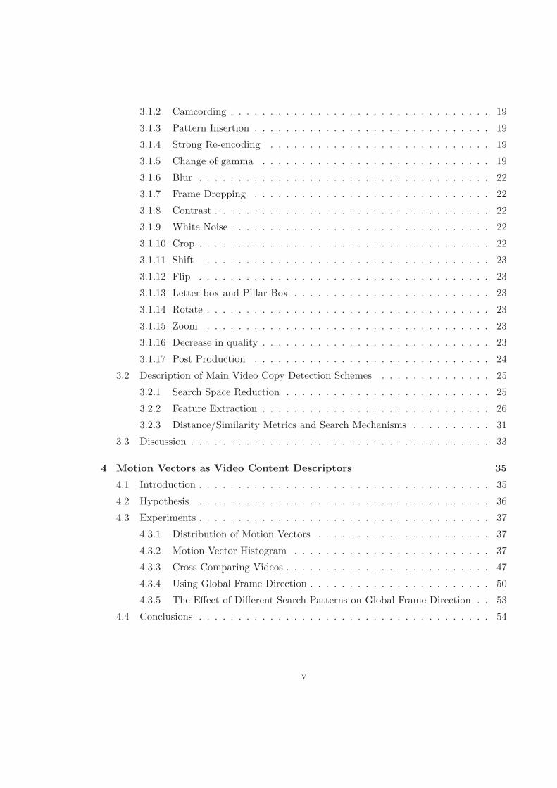
3.1.2 Camcording . . . . . . . . . . . . . . . . . . . . . . . . . . . . . . . . . 19
3.1.3 Pattern Insertion . . . . . . . . . . . . . . . . . . . . . . . . . . . . . . 19
3.1.4 Strong Re-encoding . . . . . . . . . . . . . . . . . . . . . . . . . . . . 19
3.1.5 Change of gamma . . . . . . . . . . . . . . . . . . . . . . . . . . . . . 19
3.1.6 Blur . . . . . . . . . . . . . . . . . . . . . . . . . . . . . . . . . . . . . 22
3.1.7 Frame Dropping . . . . . . . . . . . . . . . . . . . . . . . . . . . . . . 22
3.1.8 Contrast . . . . . . . . . . . . . . . . . . . . . . . . . . . . . . . . . . . 22
3.1.9 White Noise . . . . . . . . . . . . . . . . . . . . . . . . . . . . . . . . . 22
3.1.10 Crop . . . . . . . . . . . . . . . . . . . . . . . . . . . . . . . . . . . . . 22
3.1.11 Shift . . . . . . . . . . . . . . . . . . . . . . . . . . . . . . . . . . . . 23
3.1.12 Flip . . . . . . . . . . . . . . . . . . . . . . . . . . . . . . . . . . . . . 23
3.1.13 Letter-box and Pillar-Box . . . . . . . . . . . . . . . . . . . . . . . . . 23
3.1.14 Rotate . . . . . . . . . . . . . . . . . . . . . . . . . . . . . . . . . . . . 23
3.1.15 Zoom . . . . . . . . . . . . . . . . . . . . . . . . . . . . . . . . . . . . 23
3.1.16 Decrease in quality . . . . . . . . . . . . . . . . . . . . . . . . . . . . . 23
3.1.17 Post Production . . . . . . . . . . . . . . . . . . . . . . . . . . . . . . 24
3.2 Description of Main Video Copy Detection Schemes . . . . . . . . . . . . . . 25
3.2.1 Search Space Reduction . . . . . . . . . . . . . . . . . . . . . . . . . . 25
3.2.2 Feature Extraction . . . . . . . . . . . . . . . . . . . . . . . . . . . . . 26
3.2.3 Distance/Similarity Metrics and Search Mechanisms . . . . . . . . . . 31
3.3 Discussion . . . . . . . . . . . . . . . . . . . . . . . . . . . . . . . . . . . . . . 33
4 Motion Vectors as Video Content Descriptors 35
4.1 Introduction . . . . . . . . . . . . . . . . . . . . . . . . . . . . . . . . . . . . . 35
4.2 Hypothesis . . . . . . . . . . . . . . . . . . . . . . . . . . . . . . . . . . . . . 36
4.3 Experiments . . . . . . . . . . . . . . . . . . . . . . . . . . . . . . . . . . . . . 37
4.3.1 Distribution of Motion Vectors . . . . . . . . . . . . . . . . . . . . . . 37
4.3.2 Motion Vector Histogram . . . . . . . . . . . . . . . . . . . . . . . . . 37
4.3.3 Cross Comparing Videos . . . . . . . . . . . . . . . . . . . . . . . . . . 47
4.3.4 Using Global Frame Direction . . . . . . . . . . . . . . . . . . . . . . . 50
4.3.5 The Effect of Different Search Patterns on Global Frame Direction . . 53
4.4 Conclusions . . . . . . . . . . . . . . . . . . . . . . . . . . . . . . . . . . . . . 54
v

5 Proposed Algorithm 56
5.1 Algorithm Overview . . . . . . . . . . . . . . . . . . . . . . . . . . . . . . . . 56
5.2 Algorithm Details . . . . . . . . . . . . . . . . . . . . . . . . . . . . . . . . . . 57
5.3 Algorithm Analysis . . . . . . . . . . . . . . . . . . . . . . . . . . . . . . . . . 63
6 Evaluation 65
6.1 Implementation of Proposed Algorithm . . . . . . . . . . . . . . . . . . . . . 65
6.2 Video Database . . . . . . . . . . . . . . . . . . . . . . . . . . . . . . . . . . . 69
6.3 Experiments . . . . . . . . . . . . . . . . . . . . . . . . . . . . . . . . . . . . . 69
6.4 Experimental Results . . . . . . . . . . . . . . . . . . . . . . . . . . . . . . . . 72
6.4.1 Base Case . . . . . . . . . . . . . . . . . . . . . . . . . . . . . . . . . . 72
6.4.2 The Effect of Grid Partitioning . . . . . . . . . . . . . . . . . . . . . . 74
6.4.3 System Evaluation for Single Transformations . . . . . . . . . . . . . 74
6.4.4 System Evaluation for Multiple Transformations . . . . . . . . . . . . 75
6.4.5 Effectiveness of Sub-sampling . . . . . . . . . . . . . . . . . . . . . . 76
6.5 Discussion . . . . . . . . . . . . . . . . . . . . . . . . . . . . . . . . . . . . . . 78
7 Conclusions and Future Work 80
7.1 Conclusions . . . . . . . . . . . . . . . . . . . . . . . . . . . . . . . . . . . . . 80
7.2 Future Work . . . . . . . . . . . . . . . . . . . . . . . . . . . . . . . . . . . . 81
Bibliography 85
vi

List of Tables
3.1 Summary of Transformations . . . . . . . . . . . . . . . . . . . . . . . . . . . 24
3.2 TrecVid Transformations . . . . . . . . . . . . . . . . . . . . . . . . . . . . . . 24
3.3 Evaluation of features used in video copy detection. . . . . . . . . . . . . . . 34
4.1 Distance between motion histograms of the source video and transformed
video after resizing. . . . . . . . . . . . . . . . . . . . . . . . . . . . . . . . . . 45
4.2 Distance between motion histograms after blurring. . . . . . . . . . . . . . . . 45
4.3 Distance between motion histograms after cropping. . . . . . . . . . . . . . . 46
4.4 Distance Statistics between Reference Video Under Common Transformations
and Distance Statistics between each of the 399 Video Clips in the TRECVID
2009 Video database. . . . . . . . . . . . . . . . . . . . . . . . . . . . . . . . 49
6.1 Evaluation criteria for multiple transformations applied to a copy. . . . . . . 72
vii

List of Figures
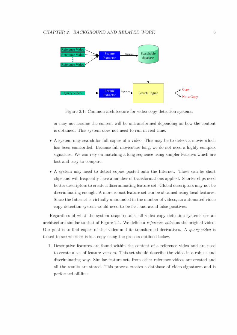
2.1 Common architecture for video copy detection systems. . . . . . . . . . . . . 6
2.2 A simple approximation for the Gaussian second order partial derivative. . . 10
2.3 The partitioning and creation of the ordinal frame signature. . . . . . . . . . 15
3.1 Images of common transformations. . . . . . . . . . . . . . . . . . . . . . . . 21
4.1 Extraction of motion vectors. . . . . . . . . . . . . . . . . . . . . . . . . . . . 38
4.2 Distribution of Motion Vectors in 3 different videos. . . . . . . . . . . . . . . 39
4.3 Screen-shot of Adobe Premiere Pro graphical interface. . . . . . . . . . . . . . 41
4.4 Histograms of various transformations applied to a single video clip. . . . . . 44
4.5 Three different logo insertions. . . . . . . . . . . . . . . . . . . . . . . . . . . 46
4.6 Signatures for two completely different videos. . . . . . . . . . . . . . . . . . . 48
4.7 Global Motion Vector Direction vs. Frame Number for Rotation and Blurring. 51
4.8 The MPEG motion vectors are dependent on the search pattern used. . . . . 54
5.1 The proposed algorithm. . . . . . . . . . . . . . . . . . . . . . . . . . . . . . . 58
5.2 The mask for a combination of PIP and letter-box transformations. . . . . . . 59
5.3 Building the ranking matrix. Each frame is divided into a 2x2 grid. The
number of SURF features are counted for each area of the grid to produce
the matrix S. The ranking matrix, λ, is built as follows: each row stores the
rank of the corresponding frame over the length of the video sequence. . . . 61
5.4 The top two rows show the ranking vectors between a query and a reference
video where the vectors are exactly opposite each other. Here, M=10 is even
and the normalization factor, C(M), is simply twice the sum of the first M/2
odd integers. . . . . . . . . . . . . . . . . . . . . . . . . . . . . . . . . . . . . 63
viii

6.1 Precision and recall curves for untransfromed videos. . . . . . . . . . . . . . . 73
6.2 The distance between queries of varying grid configurations are shown as a
function of their frame sizes. . . . . . . . . . . . . . . . . . . . . . . . . . . . . 73
6.3 Precision and Recall for 30 second query clips. . . . . . . . . . . . . . . . . . 75
6.4 The precision-recall curve for multiple transformations. . . . . . . . . . . . . . 76
6.5 Precision and recall graphs for different sampling ratios. . . . . . . . . . . . 77
ix

Chapter 1
Introduction
1.1 Overview
The first practical video recording device [42] was invented in the 1950’s. It recorded live
television onto a magnetic tape, but a price tag of $50,000 put it out of reach of the common
consumer. The early 1980’s saw the release of consumer video recording equipment in the
form of video cassette recorders (VCRs) and video recording cameras (camcorders). The
early camcorders were in the form of large, bulky, shoulder-mounted units which stored
content information directly onto VHS cassettes. Technological advances have continued
with cameras becoming smaller due mainly to replacing magnetic tape storage with solid
state storage or flash drives. Storage capacity has also increased. The information is now
recorded digitally and compression routines are applied to store the data efficiently. It is not
uncommon to find video recording capabilities bundled with other electronic devices such
as cell phones or personal digital assistants (PDAs). Meanwhile, VCRs have been replaced
by digital video recorders or DVRs. Currently, camcorders and DVR’s are readily available
and easily affordable leading to a proliferation of video recorders.
Virtually all modern video recorders store data digitally. Moreover, they are built with
connection ports to easily connect and upload the recorded content onto a computer. It
is a simple matter to further distribute the content from a computer onto social media
websites such as YouTube or facebook. More and more people are uploading and sharing
video content. This situation creates issues relating to data management.
One issue is database optimization. It is inefficient to store multiple copies of the same
video in a database as it creates needless infrastructure expenses and complicates search
1

CHAPTER 1. INTRODUCTION 2
and retrieval algorithms. If we can detect whether a video already exists in the database,
we can make more effective use of storage.
Another serious issue relates to copyright infringement. It is relatively easy to copy
commercial content and redistribute it over the Internet. This can result in loss of revenue
for a business. It is not feasible for a human to sift through the countless hours of videos
found on the Internet to see if someone has made an illegal copy. There is a real need to
use automated video copy detection techniques to detect copyright violations.
Video copy detection can also be used to monitor usage. For example, a company pays
a television channel for a commercial advertisement. It would like to monitor the channel
for when its advertisement is played and how often. It can use these data to confirm that
contract terms have been met.
There are two fundamental approaches to video copy detection. Watermarking tech-
niques embed information into the video content. This information is unique to the video
and under normal circumstances invisible. Copy detection becomes a matter of search-
ing the video content for this hidden information. This method has several disadvantages.
Legacy films which have been released without a watermark cannot benefit from this pro-
cess. There may be too many un-watermarked copies in existence which can be used as
sources for copying. Also, many video transformations affect the watermark. If the video
is copied and re-encoded in a way which changes the watermark, then it is no longer useful
for copy detection purposes.
A better approach is to extract distinctive features from the content. If the same features
can be found in the content of both videos, then one of the videos may be a copy of the
other. This is known as Content-Based Copy Detection (CBCD). The underlying premise of
Content-Based Copy Detection is that there is enough information within a video to create
a unique fingerprint. Another way to think of it is that the content itself is a watermark.
This research focuses on creating a content based video copy detection system.
1.2 Problem Statement and Thesis Contributions
The goal of the feature extraction process is to create a fingerprint of the video content
which is robust to as many video transformations as possible. The fingerprint must also
uniquely describe the content. If it is not unique, false positives may occur.
Copy detection is not as easy as it first seems. If we want to detect whether a query

CHAPTER 1. INTRODUCTION 3
video is a copy of some reference video, we could naively compare each frame of the query
with every frame of the reference, and for each frame compare corresponding pixels. There
are two problems with this approach. If there were M frames in the query and N frames
in the reference and each frame had P pixels, then the running time would be O(MNP ).
This is unacceptable for any realistic system. The second problem is that copying the videos
often transforms them in some ways. Re-encoding a video introduces quantization errors
and noise. Recording media sensor responses frequently result in gamma shifts and contrast
changes. If the video was copied using a camcorder then the angle of the camera can skew
the recording. Some transformations are intentional. To minimize download and upload
bandwidth, the video may be cropped, resized, or its bitrate may be adjusted. Edit effects
such as text, borders, or logos may be added.
A good video copy detection system will represent the content of the video by features
which are not sensitive to the transformations described above. The feature set must be
robust and discriminating.
Robustness is the ability of the features to remain intact and recognizable in the face of
encoding distortions and edit effects. A discriminable feature is one which is representative
of the video content, but unlikely to be found in videos which do not have the same content.
It will allow us to filter out videos which do not have matching content.
In addition to being robust and discriminating, the feature set extracted should be
compact. A compact signature requires less storage space and requires less computation to
evaluate how closely two signatures match. The evaluation process must be efficient and fast
to effectively determine copies in database which may contain hundreds of hours of video.
The problem statement can be expressed as: How can we describe a video in such a
way that it is discriminating, robust to transformations and edit effects, and has a compact
signature?
The contributions of this thesis can be summarized as follows:
• A comparison of existing copy detection methods is undertaken. Key concepts used
in video copy detection systems are explained. Representative features used to create
a unique signature for video content are discussed. They are categorized and the
advantages and disadvantages of these features are compared and critically evaluated.
Various distance metrics are presented based on the representation of features.
• We investigate a video copy detection system using MPEG motion vectors. These

CHAPTER 1. INTRODUCTION 4
vectors are created during video compression. Video frames are divided into 16x16
pixel blocks called macroblocks. Often there is little difference between one frame and
the next. Instead of coding a block of pixels, we can instead see if there is a similar
block in another frame. If so we can just point to its location in the other frame using
a vector to describe its position. Then the difference between blocks is encoded. This
residual uses much less space than encoding the full macroblock. This process is called
motion compensation and the vectors produced are known as motion vectors.
We discovered that while many systems can exploit motion information effectively,
MPEG motion vectors are too much a product of the encoding parameters to be
useful as a signature in the copy detection process.
• A copy detection system is proposed which leverages the discriminating ability of local
feature detection. It uses a compact signature to avoid high storage computation costs
common when using high dimensional feature vectors. The system extends the work
of Roth et al. [36] by creating a spatial-temporal ordinal signature and adopting an
L1-distance metric to evaluate matches. This system is evaluated for many common
transformations and proves to be robust.
1.3 Thesis Organization
The rest of this thesis is organized as follows. Chapter 2 provides background information
needed to understand the concepts discussed in this thesis. It will also examine other
copy detection schemes and how they are used. Chapter 3 explains common ways video
content can be transformed. It describes the main copy detection schemes as well as voting
algorithms to decide whether a video is a copy. In chapter 4 MPEG motion vectors are
evaluated to see how effectively they can describe video content. A new copy detection
scheme is proposed in chapter 5. Chapter 6 evaluates the proposed copy detection system
and chapter 7 provides conclusions as well as ideas for future work.

Chapter 2
Background and Related Work
In this chapter we begin with an explanation of the key concepts and tools used in the
development of our video copy detection system. We also discuss current algorithms and
techniques used in this research area.
2.1 Background
2.1.1 Video Copy Detection Systems
It is important to describe the content of the video in a compact way to avoid high storage
costs and to speed the search algorithm’s running time. Distinctive characteristics of the
content are described using feature vectors. These vectors are stored in a database. To
detect a copy of a video which is in the database, similar features are extracted from a
query video and compared to those within the database.
Video copy detection systems can be used for different purposes [27].
• A system can be designed to monitor a television channel to detect copies. This would
allow a company which has purchased advertising time to ensure that it is getting the
airtime it has paid for. For this case, we can assume the content will be untransformed
and will be available in its entirety. This system does not need to worry about the
robustness of the signature to transformation, but it must operate in real-time so the
signature extraction and search algorithms must be fast.
• A system may be built to eliminate redundancy within a database. This system may
5
CHAPTER 2. BACKGROUND AND RELATED WORK 6
Searchabledatabase
Feature Extractor
Reference Video
Reference Video
Reference Video
Query Video Search EngineFeature
Extractor
Signature
SignatureCopy
Not a Copy
Figure 2.1: Common architecture for video copy detection systems.
or may not assume the content will be untransformed depending on how the content
is obtained. This system does not need to run in real time.
• A system may search for full copies of a video. This may be to detect a movie which
has been camcorded. Because full movies are long, we do not need a highly complex
signature. We can rely on matching a long sequence using simpler features which are
fast and easy to compare.
• A system may need to detect copies posted onto the Internet. These can be short
clips and will frequently have a number of transformations applied. Shorter clips need
better descriptors to create a discriminating feature set. Global descriptors may not be
discriminating enough. A more robust feature set can be obtained using local features.
Since the Internet is virtually unbounded in the number of videos, an automated video
copy detection system would need to be fast and avoid false positives.
Regardless of what the system usage entails, all video copy detection systems use an
architecture similar to that of Figure 2.1. We define a reference video as the original video.
Our goal is to find copies of this video and its transformed derivatives. A query video is
tested to see whether is is a copy using the process outlined below.
1. Descriptive features are found within the content of a reference video and are used
to create a set of feature vectors. This set should describe the video in a robust and
discriminating way. Similar feature sets from other reference videos are created and
all the results are stored. This process creates a database of video signatures and is
performed off-line.

CHAPTER 2. BACKGROUND AND RELATED WORK 7
2. The query video is analyzed and its feature vectors are extracted using the same
process described above.
3. The feature vector set from the query video is compared with the signatures stored
in the database. A distance or similarity metric is used to evaluate how closely the
query matches the reference.
4. The results are either thresholded or a voting algorithm is used to decide whether or
not to report a copy.
The evaluation metrics for video copy detection are precision (Equation 2.1) and recall
(Equation 2.2).
precision =number of correctly identified copies
total number of reported copies. (2.1)
recall =number of correctly identified copies
actual number of copies. (2.2)
It is not enough to simply identify the query as a copy of the video. We must also
pinpoint its location within the reference video. A correctly identified copy will correctly
name its corresponding reference video as well as where the copy can be found in the source.
The output could look like this:
Query 2 is a copy of Reference 23. This copy is located at time 00:31:17:00.
A 100% recall rate means that all copies are detected. We can achieve this by reporting
all queries as copies. 100% precision indicates that all reported copies are actual copies.
This can be achieved by not reporting any copies. The goal of a good copy detection system
is to maximize both recall and precision. It may not be possible to achieve both 100% recall
and 100% precision. In this case we must decide which is most important: to find all copies,
or to ensure that all reported copies are actual copies.
2.1.2 Video Compression
A movie is composed of a series of frames. Each frame is a still picture. Playing the still
images quickly produces the effect of a moving picture. Typically movies are played at a
frame rate between 25 and 30 frames per second. A 1920 x 1080 picture is often encoded
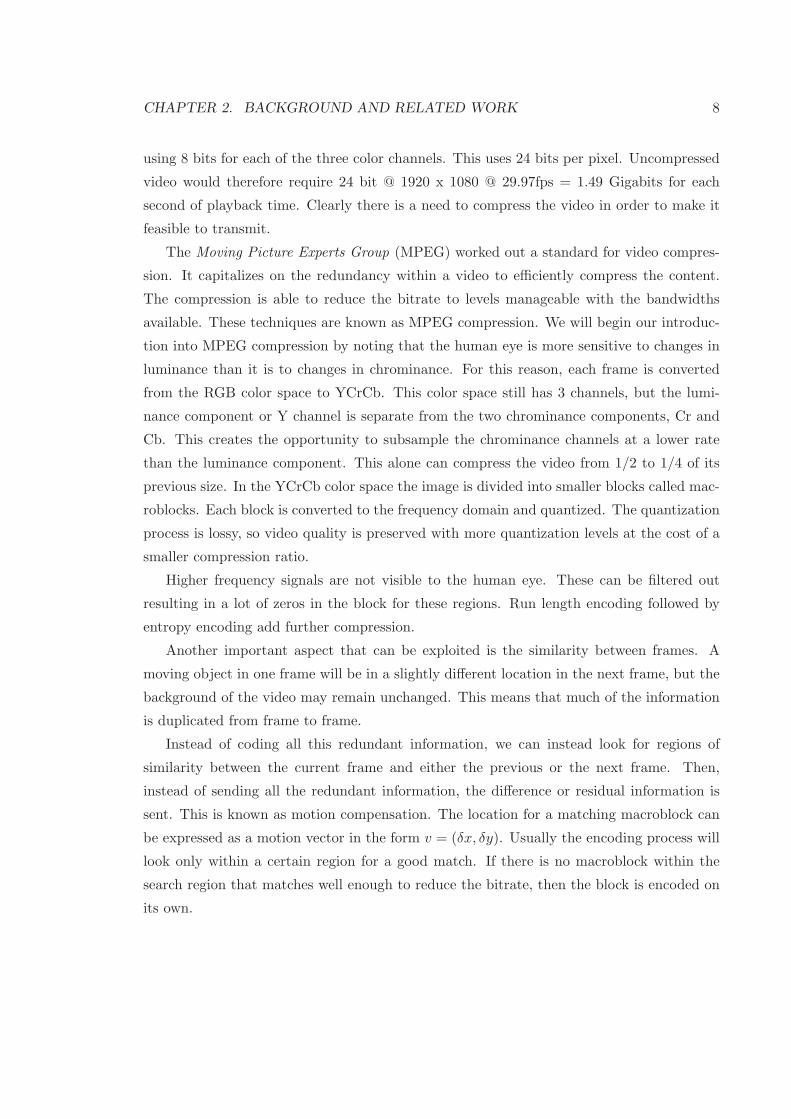
CHAPTER 2. BACKGROUND AND RELATED WORK 8
using 8 bits for each of the three color channels. This uses 24 bits per pixel. Uncompressed
video would therefore require 24 bit @ 1920 x 1080 @ 29.97fps = 1.49 Gigabits for each
second of playback time. Clearly there is a need to compress the video in order to make it
feasible to transmit.
The Moving Picture Experts Group (MPEG) worked out a standard for video compres-
sion. It capitalizes on the redundancy within a video to efficiently compress the content.
The compression is able to reduce the bitrate to levels manageable with the bandwidths
available. These techniques are known as MPEG compression. We will begin our introduc-
tion into MPEG compression by noting that the human eye is more sensitive to changes in
luminance than it is to changes in chrominance. For this reason, each frame is converted
from the RGB color space to YCrCb. This color space still has 3 channels, but the lumi-
nance component or Y channel is separate from the two chrominance components, Cr and
Cb. This creates the opportunity to subsample the chrominance channels at a lower rate
than the luminance component. This alone can compress the video from 1/2 to 1/4 of its
previous size. In the YCrCb color space the image is divided into smaller blocks called mac-
roblocks. Each block is converted to the frequency domain and quantized. The quantization
process is lossy, so video quality is preserved with more quantization levels at the cost of a
smaller compression ratio.
Higher frequency signals are not visible to the human eye. These can be filtered out
resulting in a lot of zeros in the block for these regions. Run length encoding followed by
entropy encoding add further compression.
Another important aspect that can be exploited is the similarity between frames. A
moving object in one frame will be in a slightly different location in the next frame, but the
background of the video may remain unchanged. This means that much of the information
is duplicated from frame to frame.
Instead of coding all this redundant information, we can instead look for regions of
similarity between the current frame and either the previous or the next frame. Then,
instead of sending all the redundant information, the difference or residual information is
sent. This is known as motion compensation. The location for a matching macroblock can
be expressed as a motion vector in the form v = (δx, δy). Usually the encoding process will
look only within a certain region for a good match. If there is no macroblock within the
search region that matches well enough to reduce the bitrate, then the block is encoded on
its own.

CHAPTER 2. BACKGROUND AND RELATED WORK 9
2.1.3 Visual Feature Extraction
In any image, we can define certain features. A high level example of this is if we look at
a picture of a farm, we can identify objects such as a barn, a fence, a house, a cow, etc.
With a comprehensive list of the features found within an image as well as their relative
orientations, it is possible to compare one image to another to see whether the same objects
appear in the same relative orientations. Humans seem to be able to do this instinctively.
Detection and matching of features using computers is a challenging and ongoing area of
research.
The goals in feature extraction are to detect points of interest which are reproducible
even if the image has been scaled, has had noise introduced, has been rotated, or transformed
in some other way. It is not the orientation of the image, but the relative position of the
interest points with respect to each other.
SIFT (Scale Invariant Feature Transform) and SURF (Speeded Up Robust Features) [2]
are two widely accepted feature detection systems. Both are invariant to many common
transformations, but SURF is about 6 times faster [7] in calculating interest points. The
feature vector from SIFT has 128 dimensions, while that of SURF has 64 dimensions. In
general, SIFT features are more discriminating, but harder to compute, require more stor-
age, and are more complex to compare with each other. They are well suited for object
recognition and image retrieval tasks. SURF features are popular because they are faster,
and less complex.
Any feature detection system is composed of three parts: feature selection, feature
description, and comparison of feature vectors between images to see how closely alike
they are. This research uses the SURF feature detector and focuses only on the detection
and localization of interest points.
The SURF feature detector is based on a Hessian matrix to detect blob-like structures.
Blobs are areas which are either darker or lighter than the surrounding region. A blob-like
structure is detected at points where the determinant of the Hessian Matrix is maximum.
For a particular scale, σ, it is defined as
H(x, σ) =
Lxx(x, σ) Lxy(x, σ)
Lxy(x, σ) Lyy(x, σ)
, (2.3)
where Lxx(x, σ) is obtained by convolving the image at point x with the second order

CHAPTER 2. BACKGROUND AND RELATED WORK 10
1
1
-2
1
1
-1
-1
-11 1
Lyy LxxLxy
Figure 2.2: A simple approximation for the Gaussian second order partial derivative.
derivative of the Gaussian function, ∂2
∂x2 g(σ). Points where Lxx is a minimum indicate a
transition. To speed up the calculations, simple filters are used to approximate the second
order Gaussian derivatives. Interest points are calculated at different scales to provide
robustness to scaling. Rather than resize the image, the filter size is increased. The first
iteration uses a 9x9 filter, shown in Figure 2.2 for a Gaussian distribution with σ=1.2.
With the interest points identified, a description of the neighborhood surrounding the
region is made. This description is made robust to rotation by calculating Haar wavelet
responses in the x and y directions, but storing the difference between each value with the
dominant orientation calculated by summing the responses over the neighborhood. The
neighborhood around the interest point consists of a grid of 16 sub regions centered at the
interest point. In each region the Haar wavelet response is summed in the x and y directions
as well as sums of the absolute values of the responses in both directions. Thus each of the
16 regions is described by these 4 sums, resulting in a 64-dimensional description vector.
The distance comparison metric used is simply the Euclidean distance between two vectors.
2.1.4 TRECVID
TRECVID is a conference dedicated to the evaluation of video information retrieval systems.
The name is derived in two parts. The original conference series, Text Retrieval Conference
(TREC) added a video component. According to its website [39]:
The TREC conference series is sponsored by the National Institute of Stan-
dards and Technology (NIST) with additional support from other U.S. govern-
ment agencies. The goal of the conference series is to encourage research in
CHAPTER 2. BACKGROUND AND RELATED WORK 11
information retrieval by providing a large test collection, uniform scoring pro-
cedures, and a forum for organizations interested in comparing their results. In
2001 and 2002 the TREC series sponsored a video ”track” devoted to research in
automatic segmentation, indexing, and content-based retrieval of digital video.
Beginning in 2003, this track became an independent evaluation (TRECVID)
with a workshop taking place just before TREC.
TRECVID has several divisions such as surveillance event detection, high-level feature
extraction, video searching, and content-based copy detection.
2.1.5 FFmpeg
FFmpeg [15] is a complete video processing library. It is open source software available
under the GNU Lesser General Public License or the GNU General Public License. It can
be used to programmatically decode a video and to re-encode the video using the codecs
available in its libavcodec library. This library contains an extensive selection of codecs
which allows us to encode a video to virtually any format. FFmpeg is a cross-platform
solution which is able to run on Windows, OS X, and Linux operating systems.
CHAPTER 2. BACKGROUND AND RELATED WORK 12
2.2 Related Work
A fingerprint can use global descriptors, local descriptors, or some combination of the two.
Global fingerprints are based on an entire frame. Local fingerprints are derived by finding
points of interest inside a particular frame. Law-To et al. [27] show that in general local
descriptors are more robust to transformations, but are computationally more expensive.
In matching full movies, the global descriptors are just as accurate, but much faster.
One natural aspect to exploit for copy detection purposes is the motion within a video.
We can capture the way objects or other features change from frame to frame with the
assumption that a copy would have the same objects and their motion would be similar.
Hampapur et al. [19] describe a signature based on the net motion of the video across
frames. They use optical flow which is a derivative based approach used to approximate
the motion of a local feature through a sequence of images. They select a patch in frame-t
centered at (xt, yt) and look in frame t+1 within a specified search region for a block which
has the minimum Sum of Average Pixel Differences, SAPD. The difference between the patch
location in frame t and the best match in frame t + 1 produces a 2-D displacement vector
(dx, dy), where dx = xt − xt+1 and dy = yt − yt+1. This vector is used to find the direction
of the local optical flow, θ = tan−1(dx/dy). They then convolve the test motion signature
with the motion signature for the reference video and calculate the correlation coefficient at
each point. The point in the convolution which results in the highest correlation coefficient
is considered the best match between the videos.
Since this method looks at the differences of pixels across frames, it is robust to color
changes. It will also work well for resizing since the regions of each block will be similarly
resized and should therefore result in the same or close to the same motion vector. Trans-
formations involving rotation will change the direction of the motion vectors and result in
poor results using this algorithm. Better results may be obtained by finding the global
orientation of the frame, and expressing the direction using this as the reference.
Tasdemir and Cetin [38] also use the motion vectors for the signature for a frame.
The vector is expressed in terms of polar coordinates and consists of a magnitude and a
direction. They obtain a stronger signature than Hampapur et al. [19] by using every nth
frame, n > 1. They found optimum results for n = 5. The signature for each frame is only
2 bytes. One byte for the Mean Magnitude of the Motion Vector (MMMV) and another for
the Mean Phase Angle of the Motion Vector (MPMV). Because they treat the magnitude

CHAPTER 2. BACKGROUND AND RELATED WORK 13
and directions separately, there is some information loss. It might make a better signature
to add all the vectors together and use the magnitude and direction of the resultant vector.
Both the above methods [38] [19] require that each frame be decoded and the motion
vectors between frames be calculated. This is computationally expensive. Some signatures
can be obtained directly from compressed video. This reduces the computational complexity
of the problem as no decoding is needed.
Li and Chen [28] propose a signature which can be extracted from the video while in the
compressed state. They extract I-frames from the video and divide the macroblocks into
regions of low, medium, and high frequency. The total count of non-zero DCT coefficients
for each region is normalized by the total number of macroblocks in the frame to create a
3-D vector of these counts. The vectors are added together for all I frames in the video
sequence and the resultant vector is normalized based on the number of I-frames extracted.
The signature is compared to the original by dividing each video sequence into a number of
clips and comparing them by adding together the absolute difference of the signatures for
each clip normalized to the number of clips. If the result is below a threshold, then a copy
is reported.
Zhang and Zou [53] also work in the compressed domain. They find edges in a macroblock
and use the orientation (θ) and strength (h) of edges for the video signature. They start
by extracting the I-frames of video sequence and then they compute θ and h for each
macroblock in the frame. If several blocks have the same orientation, they are collated into
one by adding the strengths together. The features are then sorted based on their strengths
in descending order. To compensate for any rotation they use the difference of orientations
between frames for the signature. The strengths of the edges based on the sorted differences
form a vector which will be used as the signature. Comparison is based on the normalized
vector difference between frame signatures.
The above two approaches show compressed domain signatures can work and are fast
and efficient. Both systems make some assumptions that limit their usefulness. First, they
both match query videos which are the same length as the reference video. This is useful in
a limited number of situations. Secondly, they assume that the number of I-frames from the
query video and the source video are the same. This is a function of the encoding parameters
and not necessarily the case. If the I-frames became misaligned, these approaches would
fail.
MPEG video compression methods predict future frames using motion vectors from

CHAPTER 2. BACKGROUND AND RELATED WORK 14
other frames. These motion vectors can be parsed from the video without fully decoding
the frame. Moreover, the computationally expensive motion vector calculation is already
done. The possibility of using MPEG motion vectors directly in the compressed domain is
explored further in section 4.
Some of the early video copy detection efforts focused on using color as the discriminatory
feature. Naphade et al. [31] proposed a system which created a histogram in the YUV color
space. The YUV color space is for our purposes used interchangeably with the YCrCb
color space. The luminance, or Y-channel, is quantized into 32 bins and each of the 2
chrominance channels, U and V, are quantized into 16 bins. Recall from section 2.1.2
that because humans are more sensitive to luminance than chrominance that the U and V
channels were sub-sampled, while the Y channel was not. For this reason, the histogram
for the luminance component is given finer granularity. Each frame in the video sequence
is represented by these three histograms. The distance between frames is calculated based
on a sliding window approach and the intersection of the histograms.
Color based signatures are very weak. Encoding or re-encoding often caused global
variations in color do to quantization parameters. Another weakness of color signatures
is that similar colors can be present in very different video clips. An example of this is
two video clips with different ocean scenes. The resultant histograms would have a high
intersection because each histogram would be predominately blue, but they would not be
copies. In general, color signatures are not robust to common color shifts and they are not
discriminating enough.
An improvement on the color histogram was to consider relative intensities of the pixel
responses instead. One such system was developed by Bhat and Nayer [3]. They divided
a frame into N = Nx x Ny blocks. For each block the average grey-scale intensity is
calculated. The results of each region are ranked to produce an N-dimensional vector S(t) =
(r1, r2, ..., rN ) for each frame t. They then ranked each region based on these values. Figure
2.3 shows that the upper right region has the highest average intensity and is assigned a
value of 1. The advantage here is that while different encoders or sensor responses may
change the actual values, the relative ranking of each region remains constant. This is a
clever way to counter the effects of a global color shift, or shifts introduced due to encoder
quantization errors. The distance between vectors in a test video T(t) of length LT and a

CHAPTER 2. BACKGROUND AND RELATED WORK 15
27 12
4514
Rank is 1
65 56
214
123
187
7 8
68
4 5
1
3
2
Figure 2.3: The partitioning and creation of the ordinal frame signature.
reference video R(t) is computed at frame t as:
D(t) =1
LT
t+LT /2∑
i=t−LT /2
‖R(i)− T (i)‖ . (2.4)
The frame, tmin for whichD(t) is minimal is the best match between R(t) and T (t). Dividing
the frames into regions allowed local information within the frame to be captured and
provided a better signature than one which captured only global frame information. This
technique is used in many copy detection schemes.
Chiu et al. [8] extract key frames from the ordinal signatures of the frames using a 9x9
Laplacian Gaussian filter and convolving it over the target video looking for local minima or
maxima. This detects interest points similar to the method of SURF. These interest points
denote signal transitions and when found are used for the key frames. The key frame is
divided into 9 regions and a 9x1 vector is used to represent the ordinal value in each region.
This becomes the fingerprint for the frame. Selection of matching clips is done in two stages.
In the first stage, two passes are made of the target clip to identify matches for the starting
and ending frames respectively. If the magnitude of the signature vector difference between
the query start (or end) frame and some target frame is smaller than some threshold, then
it is added to a list of candidate frames. Candidate clips are selected based on the candidate

CHAPTER 2. BACKGROUND AND RELATED WORK 16
start and end list which meet the criteria that the start frame comes before the end frame,
the selection is the smallest frame set possible and the number of frames is not too much
longer or shorter than the query clip. The candidate clips are evaluated for similarity with
the target based on a time warping algorithm which accounts for video temporal variations.
This provides a nice way to deal with situations involving frame dropping or videos with
different frame rates.
Kim and Vasudev [24] add a temporal component to Bhat and Naher’s ordinal signature.
The spatial signature is the same as that of Bhat and Nayer. When comparing frames
between the query file and the reference file, they use the spatial distance in equation 2.4,
but they also look at the way the distances change between the current frame and the
previous frame. If both the query and reference increase, there is no temporal distance. If
one stays the same while the other increases, the temporal distance is .5, and if one increases
while the other decreases, the distance is 1. The temporal distance between two clips is
obtained as the average temporal distance over all regions, where the temporal distance of
a region is the sum of the temporal distances that region over all frames, normalized to the
number of frames. They define their new spatial temporal distance as a weighting of the
spacial distance in equation 2.4 combined with temporal distance described above.
D = αDspatial + (1− α)Dtemporal. (2.5)
They found that α = .5 gave the best results.
Chen and Stentiford [6] take this one step further and rank blocks temporally rather
than spatially. If λk is the rank of the kth block, the distance between a query video, Vq
and a reference video, Vr is calculated as:
D(Vq, Vpr , t) =
1
N
N∑
k=1
dp(λkT , λ
kR), (2.6)
where
dp(λkq , λ
kr ) =
1
CM
M∑
i=1
|λkq (i)− λi
r(k)(p+ i− 1)|, (2.7)
and p is the frame offset for the region under investigation in the reference video. Cm is a
normalizing factor.
Adding the temporal component gives excellent results for simple transformations such
as contrast, crop, blur, letter-box, pattern insertion and zoom and improved both the recall

CHAPTER 2. BACKGROUND AND RELATED WORK 17
and precision of their test data. With larger transformations and combinations of transfor-
mations, the temporal-ordinal method outperformed the ordinal method with almost double
the precision [27]. It was also able to perform well for clips as small as just 50 frames.
Local information captured by SIFT or SURF features are much more descriptive, but
because of the high dimensionality of each feature vector and the large number of features
detected on a frame, the computational complexity of the distance matching is greatly
increased.
Roth et al. [36] use the robustness of local descriptors in their copy detection algorithm,
but they reduce the high dimensionality of the resultant vectors in the following way. They
take every frame of the source video and divide it into horizontally and vertically by four.
This forms 16 regions for each frame. They then use SURF, a local feature search, to find
local points of interest in the frame. Typical feature extraction algorithms will store for each
point of interest an n-dimensional vector describing the feature. The authors of this paper
instead choose to simply count the number of features identified in each region and use this
as the metric for copy detection. They create a database of videos and store for each video,
the pre-processed SURF count for each frame. To determine whether a query video is a
copy, they perform the same region by region SURF count for each frame in the query video
and compare this to each source video. The comparison metric is the normalize sum of the
differences in SURF counts for each region in the frame. Two frames are considered to be
a match if this normalize sum is below some threshold. A copy is reported if the longest
running subsequence of matches is above another threshold.

Chapter 3
Comparison of Existing Schemes
In this chapter we define many of the common transformations a video may undergo as
it is copied. We describe tools used to speed the detection process and then evaluate
representative video copy detection systems.
3.1 Transformations
A transformation is an operation which alters the content of the video in some way. A
tolerated transformation alters the video, but enough information is preserved that the
main information or content is still recognizable. Examples of tolerated transformations are
listed below.
3.1.1 Picture in Picture (PIP)
Picture in picture is when a still image or video is superimposed on top of another video.
This leads to two different situations:
• Type 1 Original is in front of a background video
• Type 2 Original is in the background with some other video in the foreground
From Table 3.1, these correspond to T1 and T2 transformations. The corresponding
TRECVID transformation from Table 3.2 is TV2.
In Figure 3.1(b), the building in the upper right corner is a T1 transformation, while the
driver would be T2. TRECVID puts limits on the location and the size of the embedded
18

CHAPTER 3. COMPARISON OF EXISTING SCHEMES 19
picture. It is located in one of the four corners of the background video or it is in the center
of the frame. It is also of size between 30% and 50% of the background video.
3.1.2 Camcording
Camcording (T3 from Table 3.1), see Figure 3.1(c) is re-recording video content using a
camcorder. Camcording can be used to illegally copy video by recording films from a movie
theater. It presents a special challenge because the recording may be distorted by the angle
of the camera to the screen. There are two angles to consider. The vertical angle is the
angle between the observer and the center of the film vertically. Similarly, the horizontal
angle measures the relation between the observer and the film horizontally.
3.1.3 Pattern Insertion
One of the most common video transformations is the insertion of logos or text (T4 from
Table 3.1 or TV3 from Table 3.2) onto the content as in Figure 3.1(d). Other patterns can
include putting borders around the movie clip.
3.1.4 Strong Re-encoding
To save space, video content is often re-encoded with higher compression (T5 from Table
3.1 or TV4 from Table 3.2). Typically higher frequency components are dropped and fewer
quantization levels are used resulting a better compression ratio, but with a lower quality
encoding of the content.
3.1.5 Change of gamma
The sensor responses in digital capture media are not linear, but rather exponential. The
intensity of the response is given by
Iout = Iinγ . (3.1)
For example, suppose γ = 2 and sensor1 measured a response of 4 while sensor2 recorded
a response of 16. The actual intensities at sensor1 and sensor2 are 2 and 4 respectively. When
exporting the data for display, the manufacturers automatically adjust for the gamma factor
of their device, but there is often some variance between devices. This variance is called
gamma shift (T6 from Table 3.1 or TV5 from Table 3.2). Example are shown in Figures
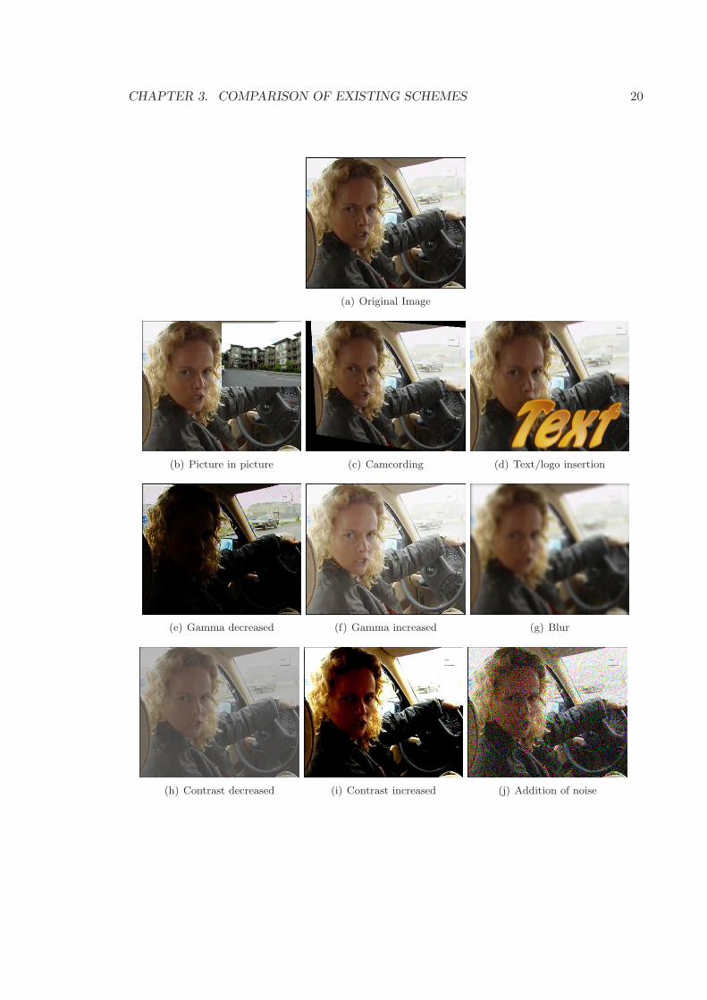
CHAPTER 3. COMPARISON OF EXISTING SCHEMES 20
(a) Original Image
(b) Picture in picture (c) Camcording (d) Text/logo insertion
(e) Gamma decreased (f) Gamma increased (g) Blur
(h) Contrast decreased (i) Contrast increased (j) Addition of noise

CHAPTER 3. COMPARISON OF EXISTING SCHEMES 21
(k) Original Image
(l) Crop (m) Shift (n) Flip
(o) Letter-box effect with stretch (p) Pillar box effect (q) Rotate
(r) Zoom
Figure 3.1: Images of common transformations.

CHAPTER 3. COMPARISON OF EXISTING SCHEMES 22
3.1(e) and 3.1(f). Gamma shifts display as an overall lightening or darkening of the video
content.
3.1.6 Blur
Blurring (T7 from Table 3.1) is often used to smooth out image noise. As we can see in
Figure 3.1(g), it results in a loss of detail. The image is blurred by convolving the image with
some averaging function. Each pixel’s value is set as a weighted average of the surrounding
pixels. Gaussian blur is most frequently used in image processing.
3.1.7 Frame Dropping
Random frames may be omitted (T8 from Table 3.1) when making a copy either intentionally
to avoid detection or as part of re-encoding.
3.1.8 Contrast
Contrast (T9 from Table 3.1) is the property of an object which makes it distinguishable
from other objects. It is affected by the color and brightness of the object relative to other
objects in the field of view. Several mathematical models for defining contrast exist. In
the YCrCb color-space, the luma component (Y) is used as a measure of the light intensity.
Contrast can be calculated as the difference in luminance over the average luminance. Thus
pixels which are close in luminance to surrounding pixels will have low contrast and will not
be as distinguishable. Figures 3.1(h) and 3.1(i) show the effects of changing contrast.
3.1.9 White Noise
White noise (T11 from Table 3.1) is introduced in such a way that it has a flat frequency
distribution. Figure 3.1(j) shows how an image can be affected with this transformation.
3.1.10 Crop
When we crop (T12 from Table 3.1) an image, we define a rectangular area inside an image
frame of the video and removes from the frame pixels which are outside this region. Figure
3.1(l) shows a cropped image. The black border around the image are the pixels which have
been removed or cropped. When cropping, it is also possible to resize the image to minimize
this border.

CHAPTER 3. COMPARISON OF EXISTING SCHEMES 23
3.1.11 Shift
The video copy has been translated (T13 from Table 3.1) either horizontally, vertically, or
both. In Figure 3.1(m), the video has been translated both to the left and up.
3.1.12 Flip
The clip is rotated around a vertical axis (T15 from Table 3.1) in the center of the frame
as shown in Figure 3.1(n)
3.1.13 Letter-box and Pillar-Box
Letter-box and pillar-box (T21 from Table 3.1) effects show up when the proportions of the
video content are different than the background screen. The pillar-box effect is common
when showing standard definition content with a 4:3 aspect ratio on a wide screen with a
16:9 aspect ratio. It is seen as black bars on the sides of the video as Figure 3.1(p) shows.
Letter-box shows as black bars above and below the content and is the result of trying to
show wide screen content in a standard 4:3 aspect ratio
3.1.14 Rotate
In this transformation (T18 from Table 3.1) the video is rotated around a point. Usually
the point of rotation is the center of the image. Figure 3.1(q) shows a rotation of 10 degrees.
3.1.15 Zoom
Zooming (T19 from Table 3.1) magnifies a section of the video so that if fills the screen. A
zoom effect is seen in Figure 3.1(q). This effect can also be accomplished by use of cropping
and scaling in combination.
3.1.16 Decrease in quality
Usually videos are altered by several transformations. A video may first have its contrast
increased 10% and then blurred using a Gaussian blur of radius 2 to smooth it out. Finally,
it can encoded at a lower bitrate to increase compression.

CHAPTER 3. COMPARISON OF EXISTING SCHEMES 24
T1 Picture in Picture — Type I T12 Crop
T2 Picture in Picture — Type II T13 Shift
T3 Camcording T14 Caption
T4 Insertion of Patterns T15 Vertical Flip
T5 Strong Re-encoding T16 Changes in Color
T6 Change in gamma T17 Scaling
T7 Blur T18 Rotation
T8 Frame Dropping T19 Zooming
T9 Contrast T20 Speed Changes
T10 Compression Ratio T21 Letter Box
T11 White Noise T22 Frame Rate Changes
Table 3.1: Summary of Transformations
TV1 Camcording
TV2 Picture in Picture
TV3 Insertion of Patterns
TV4 Strong Re-encoding
TV5 Change in gamma
TV6 Any 3 Decrease in Quality transformations
TV7 Any 5 Decrease in Quality transformations
TV8 Any 3 Post Production transformations
TV9 Any 5 Post Production transformations
TV10 Combination of 5 random transformations
Table 3.2: TrecVid Transformations
TRECVID evaluates decreases in quality by combining three (TV6 from Table 3.2) or
five (TV7 from Table 3.2) of the following transformations: blurring, gamma shifting, frame
dropping, contrast change, increased compression ratio and adding white noise.
3.1.17 Post Production
TRECVID evaluates Post Production transformations using three (TV8 from Table 3.2)
or five (TV9 from Table 3.2) combinations of cropping, shifting, text/pattern insertion,
contrast change, and vertical flipping.
CHAPTER 3. COMPARISON OF EXISTING SCHEMES 25
3.2 Description of Main Video Copy Detection Schemes
In this section we discuss techniques used in video copy detection systems to reduce the size
of the signature and to increase the speed of searching the database. A few representative
systems are categorized based on their signatures and their search algorithms. These systems
are critically examined and their strengths and weaknesses are evaluated.
3.2.1 Search Space Reduction
It is unfeasible to extract features from every frame of a query video and compare these
against every frame of the reference video. All useful copy detection systems employ some
method of reducing the search space to reasonable bounds. Some general approaches include:
1. Extract representative key-frames from the videos. These frames will be the basis of
the signature.
2. Amalgamate many frames into a clip and create a signature using the combined frames.
3. Sub-sample the frames. Use 1 frame out of every n frames for the signature.
Many Systems [28] [51] [44] [53] [14] [40] [16] [25] [11] [14] [10] extract representative
frames from the video. These key-frames are used to create the signature. Using fewer
frames speeds the extraction of features and the creation of the signature. Fewer frames
analyzed also means there is less data to store. The largest benefit is in the search phase.
Fewer frames in both the reference and query signatures can result in a significant savings
when matching video queries against a database.
The difficulty of this approach is in the selection of the key-frames. The key-frame
selection algorithm must ensure that the frame selected in the reference video matches the
key-frame selected in the copy. Failure to come up with similar subsets of frames in both
the reference and the query videos would result in the failure of the system.
Some systems [28] [53] extract just the I-frames from the video. This approach relies on
the distance between I-frames in the reference video and the source video to be the same.
Since this is a parameter which can be set users, it is not a useful method of selection.
Others [25] find frames in which there has been a sudden change in luminance.

CHAPTER 3. COMPARISON OF EXISTING SCHEMES 26
Cho et al. [11] find key-frames for which the ordinal intensity signature [3] differs. Key-
frames can also be extracted from shot boundaries [14] [10]. When shooting videos, fre-
quently the camera is stopped between different scenes or sometimes within the same scene
to show a close-up. A shot consists of all frames within one continuous camera recording
session.
Many shot detection schemes exist. Wu et al. [46] use the first frame in the shot, while
Douze et al. [14] select frames which are a set offset from the shot boundaries. This is to
avoid transitional effects such as fade-in and fade-out. Zhang et al. [51] always take the
first frame of a shot, but they also select others based on several criteria. They look at the
last frame in the shot and add the current frame to the set of key-frames if its color-based
similarity differs too greatly. They also consider common camera motions such as zooming,
where both the first and the last frame will be used as key-frames, and panning where key-
frames are selected whenever a scene is shifted by more than 30% in any direction. Wolf [44]
feels that Zhang et al.’s approach selects too many frames and use optical flow analysis to
measure the motion in a shot. He selects key-frames at the local minima of motion.
Sub-sampling [14] [50] is also often used to decrease processing time. For every time
period t, one frame is extracted and used for the signature creation process.
3.2.2 Feature Extraction
Once a set of frames has been chosen, distinguishable features are extracted from the frame
and used to create a signature for the video. We will categorize and compare several copy
detection systems based on the features they use.
Clip Based Features
Some signatures aggregate many frames into a single clip. The frames within the clip are
used collectively to derive a feature vector.
Wu et al. [46] detect shot boundaries and use the sequence of shot lengths as the sig-
nature. The author claims the sequence of shot durations is unlikely to be the same in
videos which are not copies. This is an example of a clip based approach where rather than
describing a frame, several consecutive frames are combined to produce a single signature.
Coskun et al. [12] perform a discrete cosine transform in three dimension (3D-DCT)
on the luminance component. The typical 2D-DCT transform is given the third dimension

CHAPTER 3. COMPARISON OF EXISTING SCHEMES 27
temporally. They pre-process video sequences into blocks which are 32x32 pixels and 64
frames deep. They perform a 3D-DCT on the resultant cube and extract the low frequency
components in the frequency domain. The result is a 64-dimensional feature vector which
represents all 64 frames of content. This vector can then be hashed. The hash of the
reference video and the transformed video which is a copy should hash to the same value if
their content is the same and to different values otherwise.
Li and Chen [28] extract I-frames from the video and use the DCT coefficients to create
a histogram showing the frequency distribution of the frame. They segment the video into
clips and add the histograms from all I-frames within the clip together. The signature is
the normalized frequency distribution histogram.
Global Features
Global features are used to describe the entire contents of a single frame.
Hsu et al. [20] divided the image of each frame into a number of sub-images. They used
the color histogram of each sub-image as the signature for the frame.
Many copy detection systems [45] [21] [11] [8] [27] [19] [3] [6] [12] use the luminance
or grey-scale image. Most of these systems [45] [21] [11] [8] [27] [19] [3] [6] use an ordinal
measure. They rank the luminance either temporally or spatially.
In Chapter 2.2 we discussed the luminance based ordinal method of Bhat et al. [3]. Their
signature was given a temporal component in [24] and was improved in [6] by ranking the
regions only in the temporal domain.
Law-To et al. [27] also added a temporal component to [3]. They define the global
temporal activity, a(t), as the weighted sum of the squares of the differences of the pixel in
frame t and frame t− 1.
a(t) =N∑
i=1
K(i) (I(i, t)− I(i, t− 1))2 , (3.2)
where K is a weighting factor used to enhance the importance of the central pixels and N
is the number of pixels.
Zhang and Zou [53] find edges within a frame by looking at the AC components of mac-
roblocks in the compressed video. They add the strengths of blocks with similar orientations
and then sort based on the strengths. They created a vector S(i) = (s1, s2, ..., sn), where s1
has the greatest strength.

CHAPTER 3. COMPARISON OF EXISTING SCHEMES 28
The motion signatures of Hampapur et al. [19] and Tasdemir et al. [38] were presented
earlier in Chapter 2.2. Hampapur et al. use a block of pixels and search for the best
matching location in the next frame. The sum of the average pixel differences is used to
evaluate how well blocks match. The best match is the location with the lowest sum. They
express the location of the best match as a motion vector and calculate the direction of the
motion. The signature for the frame is a histogram of these directions.
Tasdemir and Cetin find motion vectors in a way similar to [19], but they get a stronger
signature by considering every 5th frame. For their signature they use the mean magnitude
of the motion vectors (MMMV) and the mean phase angle of the motion vectors (MPMV).
Wu et al. [47] create a Self Similarity Matrix (SSM) and use this to generate a Visual
Character String (VCS). The Self Similarity Matrix provides a distance metric between every
combination of 2 frames in a video sequence. Thus the resulting matrix will be positive with
zeros on the main diagonal. The authors use a distance metric based on the optical flow as
it provides greater discriminative power [4]. They seek the motion vector which minimizes
the difference between blocks across frames. Spatial information is added by dividing the
blocks into sub-blocks and summing the optical flow values in the blocks. These are used
to create a feature vector, T. They calculate 3 SSMs for the x-direction, y-direction, and
both x and y directions using the Euclidean distance between any two vectors. The SSM
is used to create a Visual character string by placing an m x n mask over each point on
the main diagonal in the SSM. The Visual Character String is the concatenation of the
individual characters created by the mask. The length of the string will be the length of the
main diagonal. Copy detection is now based on the edit distance between visual character
strings. A character can be inserted, deleted, or substituted in one string to be transformed
to another. Each operation is assigned a cost. The cost of substitution is weighted by how
similar two characters are. Experiments showed the SSM using x-direction produced better
results which is reasonable since most motion in video’s is horizontal (panning).
Local Features
Algorithms which are based on local features identify points of interest. Points of interest
can be edges, corners or blobs. The SURF feature detector finds blobs. Another often used
feature detector is the Harris detector which detects edges and corners. Once the interest
point is chosen, the local region surrounding it is described.
Chen et al. [7] extract SURF interest points from each frame. They then track the

CHAPTER 3. COMPARISON OF EXISTING SCHEMES 29
trajectories of the points and use the trajectories for the signature. They use LSH (locality
Sensitive Hashing) to speed the search process.
Other systems [14] [10] extract SIFT features from key-frames and treat each descriptor
as a word. Because of the high dimensionality of the SIFT descriptors, the dictionary of
words would be too large to process. They use a clustering algorithm to reduce the size of the
dictionary. The goal of the clustering is to have words which are close together in the high
dimensional SIFT vector space be grouped together into a cluster. A hashing mechanism
then hashes the extracted SIFT word into the cluster of words most similar. The signature
then becomes the histogram of words found in each key-frame. It was suggested in [14] that
the number of clusters be 200,000.
Strengths and Weaknesses
Clip based approaches tend to give a signature which is more compact and therefore
requires a less complex search algorithm. The signatures are less discriminating since more
content is described at once. This makes them less reliable when the query videos are short.
Longer sequences will improve the accuracy of the search. Clip based approaches are still
useful for short queries. They can be used as a filtering stage to quickly reduce the number
of candidates videos from which to perform a more discriminating search.
The approaches of [46] [28] use shot detection to define clip boundaries. These algorithms
do not require much computational complexity, but the accuracy of the video signatures be-
come dependent on the accuracy of the shot boundary detection algorithm. Shot detection
algorithms use color changes, luminance changes, and image edge detection to find bound-
aries. They perform well for sudden shot changes, but they have a low success rate for
shot transitions involving fading or dissolving. Transformation which affect the features
used for shot detection can make these approaches fail. For example, Gaussian blurring will
make edges more difficult to detect. Gamma and contrast shifts will further exacerbate the
difficult task of detecting shots with fades and dissolves.
The shot timing signature of Wu et al. [46] claims that the shot lengths between videos
which are not copies are not likely to match. This is not necessarily true. News programs
often follow a template where they will have 60 seconds for a news story followed a 45 second
weather report, etc.
Coskun et al.’s signature [12] performs well for spatial transformations such as blurring,
changes of contrast, gamma shifts and noise, but it cannot deal with transformation that

CHAPTER 3. COMPARISON OF EXISTING SCHEMES 30
change the spatial temporal structure of the cube used to compute the 3D-DCT. Transfor-
mation such as adding patterns/logos, or picture-in-picture would change the structure and
the resultant hash.
The signature of Li et al. [28] creates a histogram of the frequency distribution. This
would be sensitive to the encoding parameters. If we wished to get a lower bitrate, we can
filter out more of the high frequency components of the video or change the quantization
levels. It is also sensitive to frame dropping or insertion.
Global features provide more discrimination than clip based features, but they require
a little more storage space. The computational cost of searching remains low. Usually
sequence matching techniques are used to determine whether a video is a copy. Law-To et
al. [27] state that using global features is faster than local features. This is because the
signature is less complex to extract and compute and also because the search algorithms
are not as complex. For long video sequences there no loss of performance.
The color signature [20] results in a compact signature and it has simple search routine,
but is sensitive to color shifts. Because color shifts are a common occurrence when copying
videos and because color signatures will not work on black and white video content, most
systems use the luminance component or grey-scale image in their analyses.
Systems can either use the grey-scale value directly [36] or more commonly the values are
ranked using an ordinal [3] [24] [6] measure. Ordinal measures are more stable to background
noise which would affect all pixels equally. There are also more robust to deviations which
affect a small number of pixels. While these few pixels may change the ranking matrix, the
larger portion of it would remain unaffected and the distances between the original and the
transformed ranking matrix would stay relatively the same.
The luminance based methods [3] [24] [6] performed poorly [27] for transformations like
cropping, zooming, pattern insertion, or letter-box and pillar-box effects.
The motion signatures [38] [19] are effective for many applications, but it is easy to see
problems with certain formats. A video clip from a newscast or interview often has little
motion. The camera is fixed and while there may be some zooming, that is likely the only
motion. It would be difficult for motion based approaches to distinguish between these
videos. They are also not robust to pattern insertions or other occlusions which block the
motion from being captured. Transformations involving rotation will change the direction
of the motion vectors and give poor results.
The motion captured in [47] is a viewpoint invariant signature. It performs well for

CHAPTER 3. COMPARISON OF EXISTING SCHEMES 31
transformations such as shift, crop, and rotation. It is also able to handle frame dropping and
does not rely on key-frame matching techniques, but since the distance metric is calculated
from all possible combinations of 2 frames, it is computationally expensive.
Local features are the most discriminating. They perform well for some of the more
difficult transformations like crop, shifting [26], occlusions, and rotations. They have a high
computational cost both in the calculation of points of interest and in searching. The feature
vector describing a local point of interest is larger which means more storage is required.
Features based on local interest points are more accurate and can effectively be used to find
short queries. Because of the high dimensionality of the feature vectors, and the number
of features located within a frame, most algorithms using local signatures try to reduce
the dimensionality through clustering algorithms. Clustering can reduce the dimensionality
while preserving the locality information.
Clustering require a representative training set to initialize the dictionary. The effective-
ness of these systems depends on the effectiveness both of the training set and the clustering
algorithm.
3.2.3 Distance/Similarity Metrics and Search Mechanisms
Signatures composed of histograms [31] will often use the histogram intersection for their
distance metric. It is defined as:
I(Ha, Hb) =L∑
i=1
min(Ha,i, Hb,i), (3.3)
where L is the number of bins in the histogram. The similarity metric is calculated as the
intersection normalized to the number of feature vectors, N , used.
S =1
NI(Ha, Hb). (3.4)
The larger the value of S, the more similar the two histograms are to each other.
Signatures composed of feature vectors are often compared using their L1 distance
(Equation 3.5) or their Euclidean or L2 distance (Equation 3.6). For two feature vectors,
v1 and v2,
DL1 =1
L
L∑
i=1
|v1(i)− v2(i)| (3.5)

CHAPTER 3. COMPARISON OF EXISTING SCHEMES 32
DL2 =
√
√
√
√
L∑
i=1
(v1,i2 + v2,i2), (3.6)
where L represents the dimensionality of the vector space. The distance will be small if the
vectors are close to each other.
Search algorithms detect copies when the similarity metric exceeds a threshold or con-
versely when the distance metric is below a threshold.
Some search algorithms used in large databases [22] [34] [37] use probabilistic search
methods. These generally are comprised of two steps. The first step is a filtering step
and the second is a refinement step. For copy detection schemes, the refinement step uses
the typical distance calculations above and does a sequential scan to discover copies. The
filtering step is used to find all elements in some hyper-volume such that
∫
Vα
p(X|Y )dV ≤ α (3.7)
where p(X|Y ) is the probability density function that the signature of X and the signature
of Y are from the same reference video, given the signature of Y . The refinement step is only
performed on the elements of the set returned by equation 3.7. Multidimensional indexing
of the database is done by partitioning the database. Joly et al. [22] use Hilbert’s space
filling curve while Poullot et al. [34] use a Z-grid partitioning scheme. Both partitionings try
to preserve the neighborhood relationships. Features from the query signatures mapped to a
partition of the database should be close to the other features in the partition. The detailed
search is only performed on the feature vectors in partitions for which a query feature vector
has been mapped. This can greatly reduce the search space if the partitioning is reasonably
uniform. As with any clustering method, there is no guarantee of this.
Gengembre and Berrani [16] do not concentrate on the selection of key-frames, but rather
on the search mechanism. They operate under the premise that if one key-frame is identified
as being similar to a key-frame in the reference video, then it is likely that the next key-
frames of both the reference and query videos will also match. They use a Bayesian filtering
approach for calculating the probabilities. The probability distribution for the kth key-frame
is derived using Bayes conditional probability from (k− 1)th probability distribution. They
call their approach a fusion model as it can be fused to any existing key-frame extraction
method to dramatically increase both precision and recall results. In section 7.2, it is
recommended that this fusion approach be added to the proposed algorithm.

CHAPTER 3. COMPARISON OF EXISTING SCHEMES 33
3.3 Discussion
Signatures which are clip based or use global motion tend to be less discriminating than local
features, but they are less difficult to compute and have simpler search algorithms. Global
signatures are often given a spatial component. Spatial signatures use the relationship of
information within a frame for the signature. This is often achieved by dividing the frame
into grids. They can also have a temporal component. Temporal signatures look at the
relationship of information along the time-line. Better results can be obtained through a
combination of both approaches. The robustness of global signatures varies depending on
the feature extracted.
Local features are more robust and more discriminating, but have high storage costs,
high computational costs, and complex search algorithms.
The type of feature to use depends on the application. To find exact copies, we do not
need to worry about robustness. To find full length movies, global features work just as well
as local features, but are significantly faster and use less storage. To find short clips, local
features are more discriminating and more robust. Table 3.3 gives an overview of some of
the systems discussed and shows their strengths and weaknesses. Refer to Table 3.1 for the
meanings of the transformations.

CHAPTER 3. COMPARISON OF EXISTING SCHEMES 34
Feature type Signature Strengths Weaknesses
Clip
Shot timings [46] T3,T4,T5, T6,T7,T8,T9T10,T12-T19 T11,T20,T22
3D-DCT [12] T6,T7,T9,T11 T1,T2,T4,T12-T15T18,T20,T21
DCT Frequency T6,T7,T9,T11 T1-T5,T8,T10Histogram [28] T22
Global
Color Histogram [20] T7,T15,T18 T1,T4,T5,T9,T11T12,T14,T16,T21
Ordinal Intensity [3] T5-T7 T4,T8,T12,T19[21] [11] [8] [19] T9-T12Temporal Ordinal T5-T7,T9-T13 T4,T8Intensity [6] [24] [27] T17,T21Motion Vector: T3,T5-T10 T4,T12,T14,T15Optical Flow [19] [38] T13,T16,T17 T18,T19,T21Motion Vector: T3,T5-T10,T12 T4,T15,T21SSM [47] T13,T16-T19Edge Analysis [53] T6,T7,T9,T17 T5,T8,T22
T19,T21
Local
SURF Trajectory T3-T14,T21and LSH [7] T16-T19SIFT [10] [14] T3-T14,T21
T16-T19
Table 3.3: Evaluation of features used in video copy detection.

Chapter 4
Motion Vectors as Video Content
Descriptors
In this chapter we investigate using MPEG motion vectors as a signature for a video. The
motion vectors are computed during MPEG compression and can be read directly from the
video file. As a result, there is little computational cost in the signature creation process.
4.1 Introduction
When presenting a moving picture to some audience, it is obvious that the motion of a
car driving across the scene is different from the motion of a ball bouncing up and down.
It makes sense that the motion of the video could be made into a unique signature for
copy detection purposes. Several systems [7] [19] [38] [44] already capitalize on this idea,
but in doing so they need to perform computationally expensive routines to identify and
quantify the motion. In Chapter 2.1, we presented an overview of how MPEG compression
works. The encoding algorithm looks at a particular macroblock and before encoding it,
searches within some reference frames for a similar macroblock. If it finds one, it stores
the location of this macroblock as a vector and encodes the difference between it and the
current macroblock. This avoids storing redundant data.
The computationally expensive search for the motion within the video has already been
performed during this encoding process. These vectors can be extracted from the video file
directly without the need to decode the entire file.
35

CHAPTER 4. MOTION VECTORS AS VIDEO CONTENT DESCRIPTORS 36
We design and conduct extensive experiments to study the feasibility of using MPEG
motion vectors for capturing the underlying motion within a video. Our goal is to use these
data to create a robust, descriptive signature that can be used to detect video copies.
4.2 Hypothesis
We propose to use the motion vector information found within compressed video content to
create a descriptive signature of the video content. These motion vectors can be accessed
without decoding the entire video. Because these motion vectors are already computed, the
computational complexity of the extraction algorithm is greatly decreased which increases
the speed of the detection process. We further propose that the generated signature will be
unique enough to identify it among a database containing signatures of many videos. We
also assume that this signature will be robust to transformations and editing effects common
when processing videos.
To validate these hypotheses, we undertake the following experiments:
• We investigate the distribution of motion vectors. We extract the motion vectors from
several videos and create a histogram of the raw data. We do this to get a sense of
what we are working with and how to use the information to create a signature.
• We create a vector-based signature using histograms. We calculate the difference
between two feature vectors using the L2-distance, which is defined in Equation 3.6.
We compare the distance found between the original video and copies of itself under
several transformations. The purpose of this experiment is to establish that comparing
the original video to a copy of itself results in a small distance.
• We create a vector-based signature using histograms. We compare the distance found
between the original video and that of videos which are not copies. The purpose of this
experiment is to establish that comparing the original video to a completely different
video will result in a large distance. This distance must be significantly larger then
the distance in the previous experiment to show good discrimination between videos
which are copies and videos which are not. We can use the results of this experiment
with the preceding experiment to determine a threshold distance. If the calculated
distance is below a threshold, then a copy is reported.
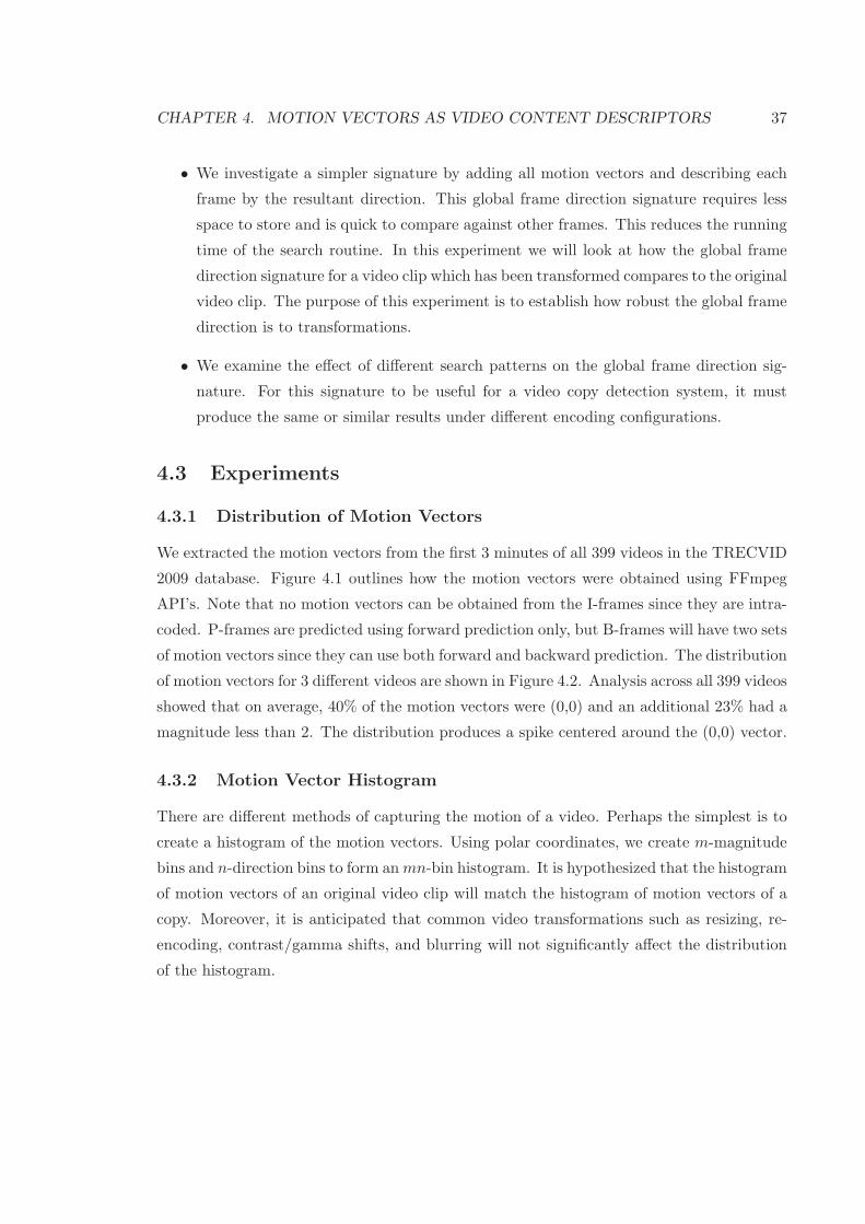
CHAPTER 4. MOTION VECTORS AS VIDEO CONTENT DESCRIPTORS 37
• We investigate a simpler signature by adding all motion vectors and describing each
frame by the resultant direction. This global frame direction signature requires less
space to store and is quick to compare against other frames. This reduces the running
time of the search routine. In this experiment we will look at how the global frame
direction signature for a video clip which has been transformed compares to the original
video clip. The purpose of this experiment is to establish how robust the global frame
direction is to transformations.
• We examine the effect of different search patterns on the global frame direction sig-
nature. For this signature to be useful for a video copy detection system, it must
produce the same or similar results under different encoding configurations.
4.3 Experiments
4.3.1 Distribution of Motion Vectors
We extracted the motion vectors from the first 3 minutes of all 399 videos in the TRECVID
2009 database. Figure 4.1 outlines how the motion vectors were obtained using FFmpeg
API’s. Note that no motion vectors can be obtained from the I-frames since they are intra-
coded. P-frames are predicted using forward prediction only, but B-frames will have two sets
of motion vectors since they can use both forward and backward prediction. The distribution
of motion vectors for 3 different videos are shown in Figure 4.2. Analysis across all 399 videos
showed that on average, 40% of the motion vectors were (0,0) and an additional 23% had a
magnitude less than 2. The distribution produces a spike centered around the (0,0) vector.
4.3.2 Motion Vector Histogram
There are different methods of capturing the motion of a video. Perhaps the simplest is to
create a histogram of the motion vectors. Using polar coordinates, we create m-magnitude
bins and n-direction bins to form anmn-bin histogram. It is hypothesized that the histogram
of motion vectors of an original video clip will match the histogram of motion vectors of a
copy. Moreover, it is anticipated that common video transformations such as resizing, re-
encoding, contrast/gamma shifts, and blurring will not significantly affect the distribution
of the histogram.

CHAPTER 4. MOTION VECTORS AS VIDEO CONTENT DESCRIPTORS 38
Algorithm 1: Motion Vector Extraction Algorithm
Input: V : Video File1 foreach AVFrame:frame in V do
2 if frame.TYPE == P or frame.TYPE == B then
3 table← table of motion vectors4 foreach Macroblock:block in table do
5 // direction==0 means forward prediction6 // direction==1 means backward prediction7 direction ← 08 x ← block.motion val[direction][0]9 y ← block.motion val[direction][1]
10 if frame.TYPE == P then
11 // P-frames only use forward predictionOutput: (x,y)
12 end
13 else
14 // B-frames use both forward and backward prediction15 for direction← 0 to 1 do
16 x ← block.motion val[direction][0]17 y ← block.motion val[direction][1]
Output: (x,y)18 end
19 end
20 end
21 end
22 end
Figure 4.1: Extraction of motion vectors.

CHAPTER 4. MOTION VECTORS AS VIDEO CONTENT DESCRIPTORS 39
−100
−50
0
50
100
−100
−50
0
50
1000
1
2
3
4
5
6
7
8
x 105
x
Distribution of Motion Vectors
y
Cou
nt
(a) Video 1
−100
−50
0
50
100
−100
−50
0
50
1000
1
2
3
4
5
6
7
8
x 105
x
Distribution of Motion Vectors
y
Cou
nt
(b) Video 2
−100
−50
0
50
100
−100
−50
0
50
1000
1
2
3
4
5
6
7
8
x 105
x
Distribution of Motion Vectors
y
Cou
nt
(c) Video 3
Figure 4.2: Distribution of Motion Vectors in 3 different videos.

CHAPTER 4. MOTION VECTORS AS VIDEO CONTENT DESCRIPTORS 40
Using this method we can perform shot detection on the video to segment it, then
aggregate the frames within each shot to create a single histogram for each shot. This results
in relatively compact signature. We will represent the histogram as an mn-dimensional
vector
H = {h1,1, h1,2, ..., h2,1, h2,2, ..., hm,n−1, hm,n}, (4.1)
where hi,j contains a count of the number of motion vectors within the ith magnitude bin
and the jth direction bin. Then we compute the Euclidean or L2-distance between a query
video Hq and a reference video Hr as
d(Hq, Hr) =
√
√
√
√
m∑
i=1
n∑
j=1
(
hqi,j − hri,j
)2. (4.2)
Video sequences which are similar should have similar histograms and result in a small
distance measurement.
Purpose
The purpose of this experiment is to find the distance between the motion vector histograms
of copies of a reference video under different transformations. Videos which are copies should
have small distances between them. We will compare the results of this section with those
in Section 4.3.3 to determine the discriminating power of this approach.
Setup and Results
Three videos from the TRECVID 2009 dataset were used to evaluate the effectiveness of
this approach. The first 3 minutes of each video was extracted and used as query videos.
This was done with FFmpeg using the following command:
ffmpeg -i ref.mpg -g 12 -bf 2 -vframes 4500 -b 1400k ref_3_minutes.mpg
The command takes an input file and applies the specified encoding parameters. Before
it can apply the parameters it must first decode the video. FFmpeg has no way of knowing
if the original encoding parameters are the same as the above. Even if they were, it is
not as simple as just truncating the file at a certain point. The frames close to the end of
the three minute mark may have dependencies on frames which will no longer be included.
Consequently it first decodes all the frames needed and then re-encodes according to the
parameters.

CHAPTER 4. MOTION VECTORS AS VIDEO CONTENT DESCRIPTORS 41
Figure 4.3: Screen-shot of Adobe Premiere Pro graphical interface.

CHAPTER 4. MOTION VECTORS AS VIDEO CONTENT DESCRIPTORS 42
Adobe Premiere Pro was used to apply various transformations to the extracted clips.
This commercially available software made it easy to transform the videos for testing. Figure
4.3 is a screen-shot showing the control for applying a Gaussian Blur to the video. Controls
for other transformations are available and just as simple to use. One downside to this
software is that there is no command line interface for batch processing.
Once the clip has been transformed, it is processed using FFmpeg’s extensive video
processing libraries. The motion vectors are extracted and used to create the histogram
described above. The magnitude and direction of a motion vector vi = (xi, yi) was calculated
as
|vi| =√
x2i + y2i , (4.3)
θ = tan−1
(
yixi
)
. (4.4)
The maximum search radius was assumed to be 80 pixels, so the range of magnitudes
varied from 0 to 80 pixels while the directions ranged from 0 to 360 degrees. The bins of
the histogram were of uniform size. The size of each bin was determined by dividing the
maximum value by the number of bins. In our experiment we used 50 magnitude bins and
8 direction bins. The histograms of the query videos were then compared to the reference
video histograms. All histograms were normalized by dividing the count in each bin by the
total number of macroblocks considered. The transformations performed were:
1. Resizing the image from 50% of its original size to 200% of the original size.
The results are summarized in Table 4.1. Note that the encoding resulted in a distance
of 0.0639 under a scaling factor of 1.0. It is natural to expect the distance to be zero
at this scaling factor, since it should produce an unaltered 3 minute extraction of the
original movie. The discrepancy can be caused by a combination of two factors:
(a) The motion prediction algorithm of our encoder may differ from that of the
source. When the video clip was re-encoded, different motion vectors were cal-
culated than in the original encoding. Different motion vectors do not change
the way the video is rendered. Using a different block for motion compensation
results in a different residual being calculated. The combination of the residual
and the macroblock pointed to by the motion vector is the same in both cases.

CHAPTER 4. MOTION VECTORS AS VIDEO CONTENT DESCRIPTORS 43
(a) Blurred Video
0 50 100 150 200 250 300 350 4000
0.05
0.1
0.15
0.2
0.25
0.3
0.35
0.4
Bin Number
Nor
mal
ized
Cou
nt
Motion Vector Histogram for Blur
(b) Blur Histogram
(c) Rotated Video
0 50 100 150 200 250 300 350 4000
0.05
0.1
0.15
0.2
0.25
0.3
0.35
0.4
Bin Number
Nor
mal
ized
Cou
ntMotion Vector Histogram for Rotation
(d) Rotate Histogram
(e) Cropped Video
0 50 100 150 200 250 300 350 4000
0.05
0.1
0.15
0.2
0.25
0.3
0.35
0.4
Bin Number
Nor
mal
ized
Cou
nt
Motion Vector Histogram for Crop
(f) Crop Histogram

CHAPTER 4. MOTION VECTORS AS VIDEO CONTENT DESCRIPTORS 44
(g) Inserted logo
0 50 100 150 200 250 300 350 4000
0.05
0.1
0.15
0.2
0.25
0.3
0.35
0.4
Bin Number
Nor
mal
ized
Cou
nt
Motion Vector Histogram for Logo
(h) Logo Histogram
Figure 4.4: Histograms of various transformations applied to a single video clip.
(b) Compression is a lossy process. To re-encode at a scaling factor of 1.0 requires
that we decode the original and re-encode it. This results in losses due to quan-
tization levels and may have an impact on the calculation of motion vectors.
We were surprised to discover that at a scaling factor of 1.0, we did not obtain the
smallest distance. While it is reasonable that the distance is not exactly zero, we
would expect that it would be the smallest out of the group.
2. Blurring the video with a Gaussian blur of 5, 10, and 15 pixels in radius.
Figure 4.4(a) shows the original video with a 10 pixel Gaussian blur applied. The
blurring process averages pixels within the specified radius using a weighting function.
In this case the weighting function is a Gaussian curve centered on the pixel being
blurred.
Table 4.2 shows the results. It is expected that blurring should have little effect on
the resultant motion since the underlying motion is not changed. We can see that as
the blurring increases, the distance decreases. This is opposite from what we would
expect.
3. Cropping the image with a border of 10, 20, 30, 40, and 50 pixels in width.
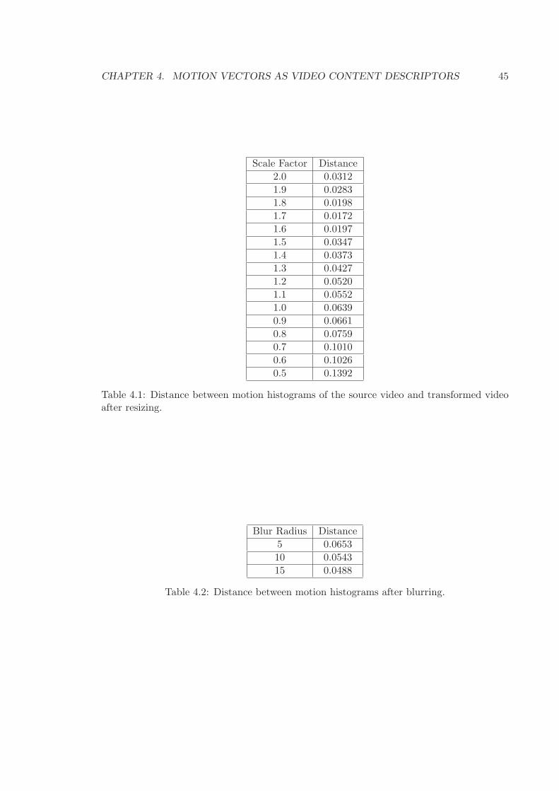
CHAPTER 4. MOTION VECTORS AS VIDEO CONTENT DESCRIPTORS 45
Scale Factor Distance
2.0 0.0312
1.9 0.0283
1.8 0.0198
1.7 0.0172
1.6 0.0197
1.5 0.0347
1.4 0.0373
1.3 0.0427
1.2 0.0520
1.1 0.0552
1.0 0.0639
0.9 0.0661
0.8 0.0759
0.7 0.1010
0.6 0.1026
0.5 0.1392
Table 4.1: Distance between motion histograms of the source video and transformed videoafter resizing.
Blur Radius Distance
5 0.0653
10 0.0543
15 0.0488
Table 4.2: Distance between motion histograms after blurring.

CHAPTER 4. MOTION VECTORS AS VIDEO CONTENT DESCRIPTORS 46
Crop Border Size Black Border Distance Resized Distance
10 0.0988 0.0836
20 0.1606 0.0801
30 0.1620 0.0762
40 0.2326 0.0785
50 0.2572 0.0706
Table 4.3: Distance between motion histograms after cropping.
(a) Logo 1 (b) Logo 2 (c) Logo 3
Figure 4.5: Three different logo insertions.
An example of a 20 pixel crop is shown in Figure 4.4(e). After cropping the video
there are two common options. The first is to simply leave the video size unchanged
by leaving a black border between the cropped area and the original video. The second
option is to resize the image to get rid of this border. In Figure 4.4(e), the video has
not been resized and black borders 20 pixels wide surround the cropped video. Table
4.3 shows that better results are achieved when the video is resized after cropping.
4. Adding a logo to the bottom of the video.
The size of each logo was not quantified in terms of area on the screen, but the first logo
had the smallest text. Logo 2 had the larger text and a small rectangular occlusion.
Logo 3 was a solid rectangle. Figure 4.5 shows an example of each logo. Resulting
distances are much larger than other transformations. This is expected as occluding
the content with a static logo prevents the underlying motion from being detected.
• Logo 1: 0.1517
• Logo 2: 0.1820
• Logo 3: 0.1520

CHAPTER 4. MOTION VECTORS AS VIDEO CONTENT DESCRIPTORS 47
5. Rotating the image from 5o to 45o in 5o increments.
Distances ranged from 0.1279 to 0.1783.
6. Varying the bitrate of the encoded video.
Distances ranged from 0.0429 at 200 kbps to 0.0734 at 8 Mbps. The distance increased
slightly with the bitrate. The source video bitrate was 1.4 Mbps.
In summary, we altered the original video by applying single transformations. The
transformations we considered were resizing, blurring, cropping, addition of a logo, rotating,
and varying the bitrate. The magnitude and direction of the MPEG motion vectors from
the transformed video were used to create a histogram. This was compared to the histogram
of the original using an L2 distance metric.
The distances for rotating the video and adding a logo were highest. This is expected
since adding a logo blocks part of the video and would change the motion vectors for the
occluded parts. Rotating the video would change the direction of all motion in the video
and the resulting MPEG motion vectors.
Cropping achieved larger distances when the region outside the crop was left as a black
border around the video. The black border region occludes the motion of the video in much
the same way as the addition of a logo did above. Resizing the video to remove this border
results in a smaller distance.
Scaling and blurring the video gave anomalous results. A scaling factor of 1.0 means
the clip was not scaled. We expect this distance to be the smallest, but all distances
with a scaling factor greater than 1.0 were smaller. A scaling factor less than 1.0 gave
expected results in that the distance measurement increased as the amount of transformation
increased. With blurring we found that as we increased the radius of the blur, the distance
decreased.
4.3.3 Cross Comparing Videos
Purpose
This experiment will evaluate the distances between different video clips. We expect that
the distance between different clips will be high. We want these data to decide a threshold
value for our system. If the distance between two videos exceeds a threshold, then a copy
is reported.

CHAPTER 4. MOTION VECTORS AS VIDEO CONTENT DESCRIPTORS 48
0 50 100 150 200 250 300 350 4000
0.1
0.2
0.3
0.4
0.5
Motion Vector Histogram for Video 1
Bin Number
Nor
mal
ized
Cou
nt
(a) Signature for Video 1
0 50 100 150 200 250 300 350 4000
0.1
0.2
0.3
0.4
0.5
Motion Vector Histogram for Video 2
Bin Number
Nor
mal
ized
Cou
nt
(b) Signature for Video 2
Figure 4.6: Signatures for two completely different videos.
Setup and Results
The first 3 minutes of the 399 clips in the TRECVID 2009 database were analyzed. The
motion vectors were extracted and used to generate the signature described in Equation 4.1.
These vectors were compared to each other to find the distance between them. Figure 4.6
shows the histograms from 2 different video clips. The Euclidean distance between these
two clips is 0.0914. Unfortunately the distance between these two unrelated clips is smaller
than the distance between many transformed copies of a video clip. There were a total of(
3992
)
= 79, 401 comparisons from which both the Euclidean and Cosine distances between
clips were considered.
We expected the distances between two completely different video clips to be greater
than the distances between the same video clip under common transformations. We can see
from Table 4.4 that this is not the case. Moreover, about 6% of cosine-distances and 5% of
Euclidean distances from completely different clips have distances better than the smallest
distance between the reference video and the transformations considered. If we tried to set
a threshold high enough to catch all the copies, then it would report a large number of false
positives. This makes the current set up unusable for a video copy detection system.
CHAPTER 4. MOTION VECTORS AS VIDEO CONTENT DESCRIPTORS 49
Cosine Distance
Reference vs. Transformed TrekVid 2009 Database
Average .0045 .0148
Minimum .0017 0.00005991
Maximum .0087 .3136
Euclidean Distance
Reference vs. Transformed TrekVid 2009 Database
Average .0985 .1398
Minimum .0017 0.00005991
Maximum .0087 .3136
Table 4.4: Distance Statistics between Reference Video Under Common Transformationsand Distance Statistics between each of the 399 Video Clips in the TRECVID 2009 Videodatabase.
Discussion
The poor results initiated further investigation into the properties of the motion vectors
themselves. To investigate further we compared the motion vectors extracted from the
original clip with ones generated during FFmpeg’s encoding process using the following
command:
ffmpeg -i MyClip.mpg -g 12 -bf 2 -vframes 4500 -b 1400k out.mpg
This command takes a source video and transcodes it to out.mpg using flags to set
encoding parameters.
• -g 12 sets the distance between I-frames to 12.
• -bf 2 sets the number of consecutive B-Frames to 2.
• -vframes sets the number of frames to encode to 4500. At 25 fps this is 3 minutes.
• -b 1400 sets the desired bitrate.
Comparing the motion vectors between clips gave interesting results. In the transcoded
clip there were some really large motion vectors. 565 motion vectors were greater than 100
in magnitude. The average magnitude of all motion vectors went from 3.97 in the original
clip to 6.54 in the transcoded clip. This is an increase of about a 64%. The average motion
CHAPTER 4. MOTION VECTORS AS VIDEO CONTENT DESCRIPTORS 50
direction was 138.90 degrees in the original clip and 145.46 degrees in the transcoded clip.
This is difference of 4.61%.
These data indicate the magnitude of the motion vectors is not a robust feature for a
video copy detection signature. Further investigation revealed that there is an additional
flag which specifies the range to search for a matching macroblock. By adding the parameter
-me_range 5,
all motion vectors were of magnitude 5 or smaller. The average magnitude was reduced to
2.25 pixels. This was a 55% difference. The average direction varied slightly. It was 144.97
degrees for a difference of 4.09%.
There are two issues here. The first is that the average magnitude can change signifi-
cantly when re-encoding a video. The second is that this magnitude is directly affected by
the parameters of the encoder. These parameters are user specified. We cannot know what
the search range is prior to creating our signatures.
Since the magnitudes of the motion vectors are a parameter of the encoding and since
users can decide the maximum magnitude to search for a matching macroblock, the resulting
histogram becomes more a function of the encoding parameters than a function of the un-
derlying motion of the video. We can conclude based on these experiments that a histogram
approach using the motion vector magnitudes from the macroblocks will be unsuccessful for
copy detection purposes
4.3.4 Using Global Frame Direction
While it has been shown above that we cannot use the magnitudes of the MPEG motion
vectors, it is still possible to use the directions.
Purpose
It was found in Section 4.3.3 that while the magnitude of the motion vectors depended on
either the default settings of the encoder or on parameters set by the user, the average
direction of the motion vectors did not change very much. The purpose of this experiment
is to create a descriptive video signature using the net direction of the motion vectors within
the frame to form a signature.

CHAPTER 4. MOTION VECTORS AS VIDEO CONTENT DESCRIPTORS 51
0 5 10 15 20 25 30 35−50
0
50
100
150
200
250
300
350
400Graph of Motion Vector Phase angles With 5 degree and 45 degree Rotation
Frame Number
An
gle
(d
egre
es)
Source Clip
5 degree rotation
45 degree rotation
(a) Rotation
0 5 10 15 20 25 30 350
50
100
150
200
250
300
350
400Graph of Motion Vector Angles with 5 Pixel Blur
Frame Number
An
gle
(d
eg
rees)
Original Clip5 Pixel Blur
(b) Blurring
Figure 4.7: Global Motion Vector Direction vs. Frame Number for Rotation and Blurring.

CHAPTER 4. MOTION VECTORS AS VIDEO CONTENT DESCRIPTORS 52
Setup and Results
If for each frame, we were to add up all the motion vectors within the frame the resultant
vector would have a direction which would represent the global direction of motion within
the frame. A long sequence of frames which matched the source video within some threshold
would indicate that the video is a copy. We define the global motion vector
Vg =(xg, yg) , where
xg =n∑
i=0
xi , and
yg =
n∑
i=0
yi,
(4.5)
where n is the number of macroblocks in the frame. The global direction for the frame is
calculated as
α = tan−1(ygxg
). (4.6)
We extracted the motion vectors from three original video clips and calculated the global
direction for each frame using Equation 4.6. We then calculated the global direction of mo-
tion for the same set of transformations in Section 4.3.2. The transformations depicted in
Figure 4.7 are rotation and blur. It is expected that blurring should have really good per-
formance because virtually nothing in the video is changed motion-wise. It is expected that
the rotated video should track the original, but with an offset roughly equal to the degree of
rotation. We can see from Figures 4.7(a) and 4.7(b) that the global frame directions of the
original video clip are not tracked at all by the global frame directions in the transformed
clips. The data for other transformations showed similar results.
Discussion
The early indications were that this would produce a more robust signature. It was suggested
that re-encoding a video sequence using different parameters for the radius of the search
pattern severely altered the resultant magnitudes, but did not have much effect on the global
frame direction. However, the results of this experiment lead us to conclude that creating a
signature using the global frame direction will not provide a robust description of the video
under common transformations. In Section 4.3.5 we will look into what went wrong.

CHAPTER 4. MOTION VECTORS AS VIDEO CONTENT DESCRIPTORS 53
4.3.5 The Effect of Different Search Patterns on Global Frame Direction
We saw that the global frame direction of transformed videos did not track that of the
original video in spite of early indications. The idea for this approach came from looking
at the directions after re-encoding the video with different search radii. We used the same
decoder/encoder for all the test transformations. As a result, we conjecture that the global
frame directions are affected in some way by the encoding parameters.
Purpose
The purpose of this experiment is to investigate the how different search patterns can affect
the global frame direction used for our signature.
Setup and Results
One way to find the best matching macroblock is to do an exhaustive search. The best
match is chosen by calculating the difference between the current block and blocks at all
other possible locations. This is computationally expensive. We can often achieve satis-
factory results with a non-exhaustive search. There are several algorithms used for motion
compensation. In a non-exhaustive search, not all locations are tested. The block matching
process will find a local minimum and not necessarily the global minimum. If we were to en-
code a video clip using different block matching search patterns, then there is no guarantee
that the resultant motion vectors will be the same. The video itself will appear identical.
If a different block is chosen for a match, then the resultant residual will also be different.
Adding the residual to the matched block will result in a correctly decoded block.
To see the effect different search patterns had on the motion vectors, the original video
was encoded using different search patterns. The patterns used are full search, hex pattern,
funny diamond, and sab diamond [15]. For each of these configurations the global direction
of each frame was calculated. In Figure 4.8 we see that the motion vectors vary significantly
under the different encodings. What we would like to see is a result similar to the first 13
frames between the funny diamond encoding and the sab diamond encoding. Both these
search algorithms produced nearly identical results initially. The overall results mean we
cannot rely on the encoder to provide the same motion vectors for the same clip. Two clips
which appear identical could be encoded using different search patterns and could have an
entirely different set of motion vectors.

CHAPTER 4. MOTION VECTORS AS VIDEO CONTENT DESCRIPTORS 54
0 5 10 15 20 25 30 35−50
0
50
100
150
200
250
300
350
400Graph showing Global Frame Direction for Differing Search Patterns
Frame Number
An
gle
(d
eg
rees)
original ClipFull SearchFunny DiamondHex PatternSab Diamond
Figure 4.8: The MPEG motion vectors are dependent on the search pattern used.
4.4 Conclusions
Using MPEGmotion vectors we quantized the vectors into a histogram of n bins. We created
a vector signature where each element of the signature corresponded to the normalized bin
count. We found that the distance between transformed copies of the same video was not
significantly less than the distances between completely unrelated videos.
While investigating why this was the case, we found that MPEG motion vectors are
affected by the radius of the search area specified in the encoding process. This limits
the radius of the search area and affects the magnitude of the resultant vectors. Thus the
magnitude of the vector becomes a function of the encoding process. Since it is not possible
to know the encoding parameters prior to copy detection, we cannot use the magnitude of
the MPEG motion vectors as part of the signature.
We thought to use the global frame direction instead. We found that the global frame
direction of transformed video clips did not match that of the original. Further investigation
revealed that the direction of the motion vector varies significantly with the search pattern
used. Identical clips encoded using different search algorithms for macroblock matching will
result in different motion vectors. The videos will decode correctly to the original clip (with
some quantization error), but the motion vectors used for prediction will be different and
therefore will point in a different direction. The result of this experiment is that we cannot

CHAPTER 4. MOTION VECTORS AS VIDEO CONTENT DESCRIPTORS 55
use the direction of a macroblock to create a signature for video copy detection.
There are other encoding parameters which may affect the resultant motion vectors.
While we have not investigated their effect, they are worth mentioning. The distance be-
tween I-frames and the number of consecutive B-frames could have an effect. Some compres-
sion routines do not use B-frames at all. This may lead to more intra-coded macroblocks and
change the distribution of motion vectors. Also worth considering is the option to encode
using one or two passes when using a variable bit rate. If there is better compression or
quality to be gained on the second pass, this could affect the distribution of motion vectors
as well.
These results do not mean that the motion of a video clip cannot be used to create a
signature. Just that the motion vectors from the MPEG motion compensation process do
not accurately capture this motion. It is important in creating a signature based on motion
between frames, that the same algorithm for calculating this motion be applied to all video
clips under consideration. In this way we can know that if the motion in one clip matches
the motion of another clip, then they are likely copies. Also, if the motion of one clip does
not match the motion of another clip, they are likely not copies.
We have studied MPEG motion vectors extensively. We conclude that there are many
parameters outside our control which directly or indirectly affect them. We therefore con-
clude that MPEG motion vectors are not useful as a signature in content based video copy
detection systems.
Chapter 5
Proposed Algorithm
In this Chapter we propose a spatio-temporal copy detection scheme which extends the
system of Roth et al. [36] by adding a temporal component to their signature. We first
present a high level overview of the concepts of the system and then delve into the details
of its implementation. Finally we analyze its running time.
5.1 Algorithm Overview
The design of a video copy detection system depends on the purpose for which it is built.
In Chapter 2.1.1 we discussed how the requirements can affect our choice in selecting the
representative features to use.
The algorithm we propose is robust to the common transformations encountered among
videos posted on social media websites such as YouTube. It is effective for databases which
comprise a few hundred hours of video content. Larger databases can benefit from probabilis-
tic approaches [34] [22] which partition the search space and only search among partitions
more likely to contain the query video. The algorithm is well suited for searching queries
which are full length copies of the original as well as for short queries.
Video signatures can be based on spatial information or temporal information. Spatial
information captures the distribution of features within a frame. Temporal information
captures movement of these features from frame to frame. A signature which incorporates
both spatial and temporal information will be more discriminative than either alone.
We propose a video copy detection system which uses a spatial-temporal signature. We
obtain the spatial information by dividing the frames of the video into regions. In each
56

CHAPTER 5. PROPOSED ALGORITHM 57
region we look for local SURF features and count the number within the region. To add
temporal information to the signature, we sort the counts in each region along the time line.
For a video of N frames, the frame with the most interest points is given a rank of 1 while
the frame with the fewest points is given a rank of N . Each region will generate its own
ranking vector, λi = (ri1, ri2, ..., r
iN ), where rij is the rank of the jth frame of the ith region.
This process is discussed more fully in Section 5.2 and can be seen graphically in Figure
5.3. The signature for the video is λ = (λ1, ..., λL), where L is the number of regions within
each frame.
We subsample the videos when creating signatures. Doing this provides smaller signature
to store and speeds the search.
We use an L1 distance metric to evaluate similarities between signatures. We analyze
the space requirements for the signature as well as its running time and we compare these
to other systems.
5.2 Algorithm Details
The proposed algorithm for video copy detection is outlined in Figure 5.1. It comprises the
following steps:
1. Remove static borders, letter-box and pillar-box effects.
This preprocessing step is done by examining how the pixels change throughout the
clip. Pixels with very low variance are likely edit effects added to the video. These
effects include borders, logos, pattern insertion as well as letter-box and pillar-box
effects from resizing.
The variance is calculated using the formula of Mark Hoemmen [41] on each pixel.
The gray-scale value of pixel x in frame i is xi.
Mk =
x1, k = 1
Mk−1 +xk−Mk−1
k , k = 2, ..., n
Qk =
0, k = 1
Qk−1 +(k−1)(xk−Mk−1)2
k , k = 2, ..., n
(5.1)

CHAPTER 5. PROPOSED ALGORITHM 58
Algorithm 2: Spatio-Temporal Video Copy Detection Algorithm
Input: Dbref : Database of signatures of reference videosInput: Vquery Query videoInput: Threshold: Threshold distanceInput: Hr, Vr: Number of Horizontal and Vertical regionsOutput: True if the query is a copy, False otherwiseOutput: Location of best match in the reference video
1 foreach Signature, Sigref in Dbref do
2 M ← Number of frames in the reference video3 N ← Number of frames in in the query video4 R←Hr∗Vr : Number of regions in each signature5 offset← 06 minDist←∞7 foreach Frame in Vquery do
8 Crop the frame to remove static borders, letter-box and pillar-box effects9 Divide into a grid of Hr x Vr regions
10 Calculate percentage of static pixels in each region11 Count the number or SURF interest points in each region12 Rank each region temporally13 Sigquery ← {r0, r1, ..., rR}, where ri is the ranking vector of the M frames of region i
14 end
15 for i← 1 to N −M do
16 foreach Usable region in the grid do
17 regionDist← 1
M
∑M
k=1|rank(Sigref (k + offset)− Sigquery(k)|
18 end
19 dist← 1
R
∑R
k=1regionDist(k)
20 offset← offset+ 121 if dist < minDist then
22 minDist← dist23 minOffset← offset
24 end
25 end
26 if minDist ≤ Threshold thenOutput: TrueOutput: minOffset
27 end
28 else Output: False
29 end
Figure 5.1: The proposed algorithm.

CHAPTER 5. PROPOSED ALGORITHM 59
(a) Video with letter-box transformation and PiP
(b) Mask of static pixels (c) Mask with Borders removed
Figure 5.2: The mask for a combination of PIP and letter-box transformations.
CHAPTER 5. PROPOSED ALGORITHM 60
Once we get to the nth frame and have calculated Qn, the variance is simply Qn/(n).
Figure 5.2(a) is an example of a video with both a letter-box and a picture-in-picture
transformation. Its mask, shown in Figure 5.2(b), is used to remove borders on the
outside of the video. The red regions are pixels whose variance is below threshold. If
all pixels in a row (or column) on the outside border have a variance below threshold,
they are removed from the image. The process is repeated until a row (or column) is
encountered where at least one pixel shows variance above the threshold. The result is
an image which is cropped of borders in which the pixels do not vary. The sub-image
corresponding to the size of the cropped mask in Figure 5.2(c) is used for further
processing. This will remove any pillar-box effects, letter-box effects, and borders
from cropping or shifting.
2. Divide the video into regions.
This is a configurable parameter. We can set the number of regions by specifying the
number of vertical and horizontal partitions. For example, specifying 3 horizontal and
2 vertical partitions would divide the frame into a grid with 3 rows and 2 columns for
a total of 6 regions.
3. Calculate the percentage of static pixels in each region.
Each region is examined for static pixels. The presence of static pixels within the
cropped image can indicate the presence of an image, some text, a logo, or a back-
ground pattern superimposed onto the video. If a significant number of pixels within
a region are masked then too much of the area may be occluded to get useful informa-
tion. If this is the case, the region can be turned off. The distance will be calculated
based on the remaining regions. In Figure 5.2(c), we can detect the presence of a
picture in picture transformation shown in red. If the percentage of red pixels in a
region is too high, then that region is not used in the distance calculation.
4. Get the spatial information for the signature.
The SURF features for the frame are extracted. Each interest point is described using
a 64-dimensional vector, but we are only interested in the location of the interest point
in the frame. We determine which region the interest point belongs to and increment
the count for that region. The top of Figure 5.3 shows how the spatial information
looks for a video with 4 frames divided into 4 regions.

CHAPTER 5. PROPOSED ALGORITHM 61
27 12
214
32 16
527
36 23
125
32 8
321
Frame 1 Frame 4Frame 3Frame 2
Rank is 4 Rank is 2 Rank is 1 Rank is 3
4
3
4
3
2
1
1
1
2
4
4
3
2
λ =
2 1 327
S =
32 36 32
12 16 23 8
14 27 25 21
2 5 1 3
Figure 5.3: Building the ranking matrix. Each frame is divided into a 2x2 grid. The numberof SURF features are counted for each area of the grid to produce the matrix S. The rankingmatrix, λ, is built as follows: each row stores the rank of the corresponding frame over thelength of the video sequence.
5. Add temporal information to the signature.
The temporal aspect of the signature is obtained by sorting the SURF feature counts
in each region along the time-line. The frame with the most SURF interest points
is assigned a rank or ordinal value of 1. The frame with the next highest number of
interest points is assigned a value of 2, and so on. Figure 5.3 provides an example of
the signature creation process. The end result is a matrix where each row corresponds
contains the ranking vector of a particular region.
More formally, for a video consisting of M frames and L regions, each region ti would
result in an M -dimension vector, si = (fi,1, fi,2, ..., fi,M ), where fi,k is the number of
SURF features counted in region i of frame k. The matrix Si = (s1, s2, ..., sL) is used
to produce the ranking matrix, λ=(λ1, λ2, ..., λL). Each λi = (ri1, ri2, ..., r
iL), where rik
is the rank of the ith region of frame k.
For a video with M frames and L regions, the signature for the video will consist of
an LxM matrix.
6. Calculate the distance between two signatures.
CHAPTER 5. PROPOSED ALGORITHM 62
The distance between a reference video and a query video is based the L1 distance
between the two. Our general approach will be this. The number of frames in the
reference video is N and the number of frames in the query video is M , where N ≥M .
We have divided the video into L regions.
We will adopt a sliding window approach. First we will calculated the distance between
the query video and the first M frames of the reference video. We will then slide our
window of M frames over one frame and find the distance between the query video and
M frames in the reference video starting at the second frame. We will keep track of
the minimum distance and the frame offset, p, for which this occurred as we continue
sliding our window. Once we reach the end of the reference video, the best match
occurs at the minimum distance.
If λi is the ranking vector of the ith region, the distance between a query video of M
frames, Vq and a reference video, Vr is calculated as:
D(Vq, Vr) = argminp
( D(Vq, Vpr ) ), (5.2)
where p is the frame offset in the reference video which achieved this minimum and
represents the location of the best match between the query video and the reference.
D(Vq, Vpr ) =
1
L
L∑
i=1
dp(λiq, λ
ir), where
dp(λkq , λ
ir) =
1
C(M)
M∑
j=1
|λkq (j)− λj
r(k)(p+ j)|. (5.3)
C(M) is a normalizing factor which is a function of the size of the query. It represents
the maximum possible distance between the reference video and the query video. This
maximum distance occurs when the ranking of the reference video is exactly opposite
to that of the query. There are two cases based on whether M is even or odd. The
case when M is even is illustrated in Figure 5.4. It is the sum of the first M/2 odd
integers. Similarly, when M is odd, C(M) is the sum of the first (M − 1)/2 even
integers. Each of these sequence can be computed directly as shown in equation 5.4.
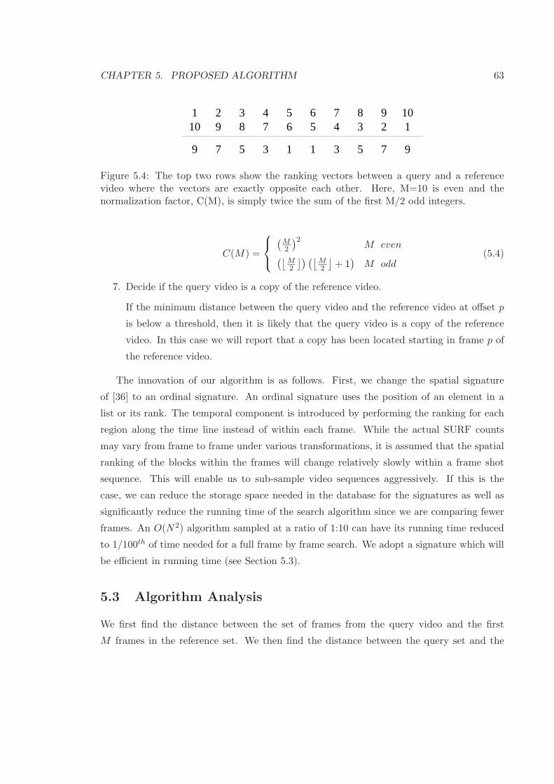
CHAPTER 5. PROPOSED ALGORITHM 63
10 9 8 7 6 5 4 3 2 1
9 7 5 3 1 1 3 5 7 9
1 2 3 4 5 6 7 8 9 10
Figure 5.4: The top two rows show the ranking vectors between a query and a referencevideo where the vectors are exactly opposite each other. Here, M=10 is even and thenormalization factor, C(M), is simply twice the sum of the first M/2 odd integers.
C(M) =
(
M2
)2M even
(⌊
M2
⌋) (⌊
M2
⌋
+ 1)
M odd(5.4)
7. Decide if the query video is a copy of the reference video.
If the minimum distance between the query video and the reference video at offset p
is below a threshold, then it is likely that the query video is a copy of the reference
video. In this case we will report that a copy has been located starting in frame p of
the reference video.
The innovation of our algorithm is as follows. First, we change the spatial signature
of [36] to an ordinal signature. An ordinal signature uses the position of an element in a
list or its rank. The temporal component is introduced by performing the ranking for each
region along the time line instead of within each frame. While the actual SURF counts
may vary from frame to frame under various transformations, it is assumed that the spatial
ranking of the blocks within the frames will change relatively slowly within a frame shot
sequence. This will enable us to sub-sample video sequences aggressively. If this is the
case, we can reduce the storage space needed in the database for the signatures as well as
significantly reduce the running time of the search algorithm since we are comparing fewer
frames. An O(N2) algorithm sampled at a ratio of 1:10 can have its running time reduced
to 1/100th of time needed for a full frame by frame search. We adopt a signature which will
be efficient in running time (see Section 5.3).
5.3 Algorithm Analysis
We first find the distance between the set of frames from the query video and the first
M frames in the reference set. We then find the distance between the query set and the

CHAPTER 5. PROPOSED ALGORITHM 64
reference set starting at the second frame of the reference set. We continue for a total of
N −M + 1 calculations. For every calculation, we compare the M frames in the query
with M frames of the reference video for a total of (N −M + 1)M comparisons. The total
running time is thus O(NM −M2 +M). As the ratio of the number of frames in the query
to the number of frames in the reference file M/N increases, the proposed algorithm will
run faster, achieving its best running time as M/N approaches 1. In this case it becomes
O(M) which means the proposed algorithm would be ideal for finding full length videos.
Small queries also run very fast. Taking the derivative of the running time and setting it
equal to zero, we see that that the worst running time is achieved when M ≈ N2 . Around
this region our algorithm has a running time of O(M2) and will greatly benefit from search
space reduction techniques.
Our algorithm has a similar running time as other algorithms [3] [9] [19] [31] which use
a sliding window approach.
It has a better running time than searches which compare frames pairwise such as [38]
[36] [47] [14]. They find the distance of all possible pairs between the query set and the
reference set. Since each frame of the query set must be compared to each frame in the
reference set, their running time is always O(MN). Note that N ≥ M . The proposed
method will always be faster since we are always subtracting M2 from the running time of
O(NM). This makes little difference when M is small, but can reduce the running time to
O(M) as M/N approaches 1.
Wu et al. [46] build a suffix array which can search in O(N), where N is the number of
key-frames extracted. Their method partitions the video into shots using a shot detection
algorithm. The duration of each shot is recorded and the signature is the sequence of shot
durations. Shot detection algorithms perform poorly when the transitions are gradual or
when there is a lot of camera motion. This signature is not very discriminating and does
not work well for short query videos.

Chapter 6
Evaluation
6.1 Implementation of Proposed Algorithm
We have implemented the proposed algorithm using Java. Below are the implementation
details of each step of our algorithm.
1. Remove static borders, letter-box and pillar-box effects.
Prior to creating our signature, we wish to remove content which is not part of the
video itself. This content can be either the letter-box or pillar-box effects described
in Chapter 3.1, or it can be a border or pattern added to the outside of the video.
We calculate the variance of pixels using Equation 5.1. There is no need to examine
every frame for this calculation, We calculate the variance by sampling 1 frame every
second. This requires that we decode the video in order to get the frame information.
We use Xuggler [48] for this purpose. It has an IMediaReader object which reads the
video stream. A listener is added to this object which invokes the callback function
onVideoPicture() once it has decoded a frame.
IMediaReader reader;
reader.setBufferedImageTypeToGenerate(BufferedImage.TYPE_3BYTE_BGR);
reader.addListener( listener );
while (reader.readPacket() == null){
}
65

CHAPTER 6. EVALUATION 66
public void onVideoPicture(IVideoPictureEvent event){
handleFrame( event.getImage() );
}
The event.getImage() method will result in a BufferedImage object. This object gives
us access to the RGB pixel values of the image. With the variance of each pixel
calculated, we start at the top of the image and look for an entire row with variance
below a threshold. We have set the threshold at 15. We continue until we can find
no more rows composed entirely of static pixels and mark the index of the row. We
do the same starting at the bottom row and working up and for the left and right
sides working inward. The image is then cropped of its static content by defining a
sub-image based on the indices found above.
image=image.getSubimage(topIndex,botIndex,leftIndex,rightIndex);
2. Divide the video into regions.
We specify the number of horizontal and vertical partitions to use. We can find the
pixel width and height of the image using
imageWidth=image.getWidth();
imageHeight=image.getHeight();
To find the pixel width of each region, we divide the pixel width of the image by the
number of vertical partitions. We use the same process to find the vertical height of
each region.
regionWidth=imageWidth/verticalPartitions;
regionHeight=imageHeight/horizontalPartitions;
A pixel with coordinates (x, y) would be in region ( xregionWidth ,
yregionHeight) in the
resulting grid.
3. Calculate the percentage of static pixels in each region.

CHAPTER 6. EVALUATION 67
We previously calculated the variance of pixels within the image. Now that we have
the image divided into regions, we look at the variance of pixels within each region. If
more than 50% of the pixels are static, then we do not use this region for our distance
calculation. This is because too much of the region is occluded.
4. Count the number of SURF interest points in each region.
We use an open source SURF feature extractor called jopensurf [23] to identify the
local features within the frame. We pass in our BufferedImage and are returned a list
of SURF interest points.
Surf surf = new Surf(image);
List<SURFInterestPoint> list=surf.getDescriptorFreeInterestPoints();
for(int i=0; i<list.size(); i++){
x = (int)list.get(i).getX();
y = (int)list.get(i).getY();
incrementSurfCount( x,y );
}
For each point in the list, we find its x and y pixel location. The method incrementSur-
fCount() will use these locations to determine which region the pixel belongs to and
will increment its count.
5. Create the signature.
The number of SURF interest points detected is stored in a 2-dimensional integer
array. The first dimension indexes the frame and the second indexes the regions. We
wish to sort the array by the number of SURF features detected and use the sorted
array to rank the frames.
We do this for each region by defining a key-value pair where the key is the frame
number and the value is the number of SURF features detected in that region. The
results are then sorted by their values in descending order so the first key-value pair
will have the most interest points.
We create a new integer array equal to the number of frames. We extract the key of
the first pair and use it to index into the new array. We assign this location a rank of
CHAPTER 6. EVALUATION 68
0. The key from the next pair is used as an index and the value of the array at this
index is assigned a rank of 1. The rest of the key-value pairs are treated similarly.
The end result is a ranking array for the region. We do this for the other regions to
create a 2-dimensional integer array where the first dimension indexes the region and
the second indexes the frame.
6. Calculate the distance between two signatures.
The signature of the query video will have fewer frames than the signature of the
reference video. If there are M frames in the query, we compare the signatures by
creating a window in the reference video of size M starting at the first frame. This
window will slide across the reference video until it reaches the end. At each location
the query video is compared to the window in the reference video. To do this, the
ranking matrix of the reference video will need to be adjusted so that frames within
the window are ranked from 0 to M − 1. This is so we can normalize the distances for
later evaluation.
We do this using a TreeMap data structure. This structure is implemented using a
red-black tree which guarantees a O(log n) cost of additions and removals. Elements
are added to the tree as a key-value pair. The tree orders its elements based on the key.
Elements are added to the tree using the ordinal rank as the key and the frame number
as the value. This way the ordinal ranking in the sliding window is maintained. As
the window slides across, the lowest frame number of the reference video is removed
at a cost of O(log M) and the next frame from the reference signature is added at a
cost of O(log M). The values elements can be extracted in O(M) time by
Collection<Integer> list=treeMap.values();
The list contains frame numbers from the reference video, where the first frame number
in the list has the highest rank. These frames are re-ranked from 0 to M − 1 and the
distance between the query and the reference window is calculated using Equation 5.3.
The best match between the two videos occurs at the frame offset with the smallest
distance.
7. Decide if the query video is a copy of the reference video.

CHAPTER 6. EVALUATION 69
We will report a copy if the best match between two videos is smaller than a threshold.
Experimentation will determine exactly what this threshold should be.
6.2 Video Database
The videos used for experimentation and evaluation come from the TRECVID [39] database.
These videos were provided by the Netherlands Institute for Sound and Vision. The videos
vary in size from 50 seconds to over 112 hours. They are stored in MPEG-1 format at 352 x
288 pixels. Altogether, there are 399 videos totaling 107 GB of data. This amounts to over
180 hours of content and over 13 million frames. The videos are encoded at a frame rate
of 25 frames per second. The database contains a wide variety of video sequences including
newscasts, documentaries, interviews, educational programming and sporting events.
6.3 Experiments
In order to evaluate our video copy detection system, we undertake the following experi-
ments:
• We first would like to test our system for the base case to determine if our system can
detect untransformed copies of a video. We randomly chose 7 videos from the TrecVid
database and used Adobe Premiere Pro to create 30 second query videos. The queries
were compared to all videos in the database.
• According to the algorithm described in Chapter 5.2, each frame is divided into a
number of regions. We investigate how the number of regions affect the distance
calculations between re-encoded copies of a video. The purpose of this experiment is
to see if the discernibility of our algorithm changes through varying the number of
regions.
Three different configurations were evaluated:
1. A 4x4 grid of 16 regions
2. A 3x3 grid of 9 regions
3. A 2x2 grid of 4 regions

CHAPTER 6. EVALUATION 70
For each configuration, query videos of size ranging from 50 frames to 5000 frames
were created from 7 random videos. The queries were created by removing the first
4000 frames from each of the reference videos, keeping the next x frames, where x is
the number of frames in the query, and discarding the rest. No transformations were
applied. In this case, we might expect that the distance between the source and the
query would be zero, but this is not the case. The reference video must be decoded and
re-encoded. Not only is this process lossy, but different encoders encode differently
based on their implementation and input parameters.
For a given query length of x frames, its corresponding reference was scanned to find
the frame offset which produced the minimum distance. The average of these distances
was calculated.
• In this experiment we evaluate the robustness of our system to various transformations.
We wish to show that with proper thresholding our system can be an effective tool for
video copy detection.
Using the same 7 videos above, several transformations were applied using Adobe
Premiere Pro for editing and Adobe Media Encoder to encode the transformed video.
The query length was kept constant at 750 frames, which is the minimum length
used by TRECVID in their evaluation process. The following transformations were
individually applied and used to evaluate the effectiveness of this approach.
– Gaussian blur of 3 pixels in radius
– Gamma shift to 0.5
– Gamma shift to 1.6
– Image rotation by 10o
– Image shift by 50 horizontally and 40 pixels vertically
– Image crop of 20 pixels from all sides
– Addition of random noise to 20% of the pixels
– Addition of text
– Image height scaled by 75% creating both a horizontal stretch and a letter-box
effect
– Camera angle adjusted by 20o horizontally and 20o vertically

CHAPTER 6. EVALUATION 71
– Image resize to 50% of its original size
– Image resize to 200% of its original size
– Contrast decreased 30%
– Contrast increased 30%
– Zoomed to 125%
– Flipped along vertical axis centered horizontally on the video
Including the untransformed clips, a total of 119 query videos were tested. The mag-
nitude of each transformation is set to the maximum used in TRECVID’s evaluation
criterion for that transformation. The exceptions are gamma shift, where TRECVID
uses 0.3 and 1.8 for their limits and resizing, where TRECVID scales down to 30% of
the original size. In these cases, our system was not able to locate copies. Gamma
shifting to the TRECVID levels is an extreme transformation and while useful in
benchmarking, it is unlikely to be used. The quality of the clip is beyond accept-
able levels for human enjoyment. It is more likely that a resize of 30% would occur for
picture-in-picture T1 transformation. Many systems are not able to cope with resizing
to this level. It is common to keep in the database both the signature of the original
video and one which has been resized. We may fail to find the query by comparing
against the full-sized version, but we will likely find it in the scaled down version.
Each transformation was compared to every reference video for the frame offset which
returned the minimum distance. An offset of zero would indicate the best match
between the query and reference frames occurs at the first frame of the reference
video.
• We also evaluated the robustness of the system to multiple transformations. For the
set of videos above we combined 3 different transformations in various configurations.
In total we tested 10 of these combinations on each of the 7 videos, creating a total of
70 transformed videos. Table 6.1 summarizes the set of transformation used and their
parameters. These results are analyzed separately from the single transformation case
above.
• In this experiment the effect of sub-sampling was examined. The purpose of this
experiment is to show that the system is able to effectively find copies under different

CHAPTER 6. EVALUATION 72
Combination Transformations
1 2 pixel blur contrast +20% letter-box
2 5% crop 10% noise gamma shift to 0.8
3 10% noise text insertion 3 pixel Blur
4 scale 120% horizontal flip rotate 5o
5 camcording 15o - 15o pillar-box contrast -20%
6 shift (20,10) rotate 10o horizontal flip
7 gamma shift to 1.3 camcording 20o - 20o contrast -30%
8 scale 75% 5% crop shift (50,30)
9 text insertion stretch letter-box
10 20% noise horizontal flip 5% crop
Table 6.1: Evaluation criteria for multiple transformations applied to a copy.
sub-sampling strategies. We created signatures by sub-sampling at ratios of 1:10 and
1:6. A ratio of 1:10 means that 1 frame out of every 10 is selected and used in the
signature creation process. The results were analyzed for precision, recall and running
time.
6.4 Experimental Results
6.4.1 Base Case
Purpose
The purpose of this experiment is to test the effectiveness of our system on untransformed
copies. 7 query videos were made using a query length of 750 frames. The TRECVID
evaluation criterion uses a minimum query length of 30 seconds [36]. This is 750 frames at
25 frames/second.
Results
We see from Figure 6.1 that we can achieve 100% precision and 100% recall in the base case
using threshold distance value in the range of 0.2320 to .2840.

CHAPTER 6. EVALUATION 73
0 0.1 0.2 0.3 0.4 0.5 0.6 0.7 0.8 0.9 10
0.1
0.2
0.3
0.4
0.5
0.6
0.7
0.8
0.9
1
Precision and Recall vs. Distance Threshold
Distance Threshold
Prec
isio
n/R
ecal
l (%
)
Precision
Recall
Figure 6.1: Precision and recall curves for untransfromed videos.
0 500 1000 1500 2000 2500 3000 3500 4000 4500 50000.05
0.1
0.15
0.2
0.25
0.3
0.35
0.4
0.45Distance vs Number of Query Frames for Various Grid Patterns
Number of Query Frames
Dis
tance
2x2 Grid3x3 Grid4x4 Grid
Figure 6.2: The distance between queries of varying grid configurations are shown as afunction of their frame sizes.

CHAPTER 6. EVALUATION 74
6.4.2 The Effect of Grid Partitioning
Purpose
In this experiment we want to determine the best grid configuration to use. Using more
regions will increase the running time, but may offer greater discrimination in detecting
copies.
Results
It was found that the best signature used a 2x2 grid for a total of 4 regions. For queries less
than 300 frames, more regions resulted in smaller distances with less variance, but as shown
in Figure 6.2, the 2x2 grid performs slightly better for queries greater than 300 frames. We
also see that longer sequences achieve better results. In this region, the 2x2 grid marginally
outperforms the other two. Consequently all future experiments will use this configuration.
The rationale is that as sequences get longer, the results get better, so we can expect more
accuracy for longer sequences.
6.4.3 System Evaluation for Single Transformations
Purpose
The purpose of this experiment was to evaluate how well our system is able to detect copies.
In this case we only apply one transformation to the copy. The decision of whether to report
a video as a copy or not is based on the distances between the query and the reference video.
In order for our system to be effective, the distance between a video and its copy must be
smaller than the distance between unrelated videos.
Results
Each transformation was compared to every reference video. This returned the minimum
distance value and the location of the copy within the reference video. These data were
used to produce the precision-recall graph in Figure 6.4.3 using Equation 2.1 and Equation
2.2.
This chart can be used by users of our system to configure the threshold. At a threshold
of 0.2830, it can still achieve 100% precision with 77% recall. The point of intersection of the
precision and recall curves occurs at a threshold of 0.3010 where both recall and precision

CHAPTER 6. EVALUATION 75
0 0.1 0.2 0.3 0.4 0.5 0.6 0.7 0.8 0.9 10
10
20
30
40
50
60
70
80
90
100
Distance Threshold
Prec
isio
n/re
call
(%)
Precision and Recall vs Distance Threshold
Recall
Precision
Figure 6.3: Precision and Recall for 30 second query clips.
are at 85%. Lowering the threshold gives greater precision, but more copies go undetected.
Raising the threshold catches more copies, but false positives are reported.
6.4.4 System Evaluation for Multiple Transformations
purpose
The purpose of this experiment was to evaluate how well our system is able to detect copies
altered by applying multiple transformations.
Results
In Figure 6.4 we see that the best recall for 100% precision is 64%. This is achieved using
a threshold of 0.2900. The intersection point occurs at a threshold of 0.3120. Here the
precision and recall are 71%. We see that we need a higher threshold to maintain the same
precision when dealing with multiple transformations. We also see that the recall rate for the
same precision is lower. This is expected behaviour, since the more the video is transformed,
the less it resembles the original, and the greater the distance between them.

CHAPTER 6. EVALUATION 76
0 0.1 0.2 0.3 0.4 0.5 0.6 0.7 0.8 0.9 10
0.1
0.2
0.3
0.4
0.5
0.6
0.7
0.8
0.9
1Precision and Recall vs. Distance Threshold
Distance Threshold
Prec
isio
n/re
call
(%)
Precision
Recall
Figure 6.4: The precision-recall curve for multiple transformations.
6.4.5 Effectiveness of Sub-sampling
Purpose
We wish to show that we can reduce the search space between a query video and a reference
video by sub-sampling the frames used for comparison. This will speed the search phase of
our system. In order for this to be effective, the system must deliver substantially the same
results using sub-sampling as without.
Results
Calculating the distances without sub-sampling took 16 hours to process. Using a sampling
ratio of 1:10 reduces the running time to around 18 minutes. In Figure 6.5 the precision and
recall are shown for different sampling ratios. The intersection point for the precision and
recall graph for a sampling ratio of 1:10 is 78%. The result is not as good as the unsampled
case, but the speed may be the deciding factor. This is a user configurable parameter, so the
sample rate can be chosen based on the whether speed or accuracy is more important. A
ratio of 1:6 reduced the time to around 46 minutes. At this rate, it takes around 40 seconds
per query to search the entire database. The results for this sampling rate are virtually the
same as for the unsampled case.
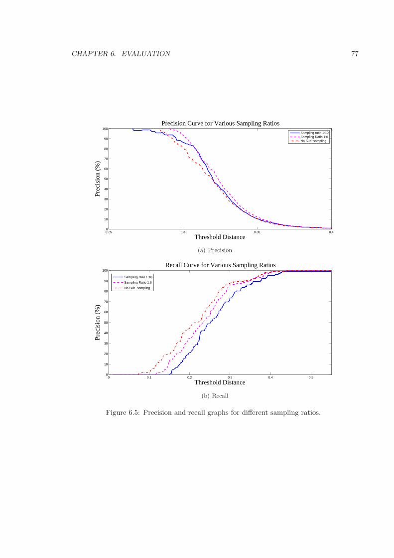
CHAPTER 6. EVALUATION 77
0.25 0.3 0.35 0.40
10
20
30
40
50
60
70
80
90
100
Threshold Distance
Prec
isio
n (%
)
Precision Curve for Various Sampling Ratios
Sampling ratio 1:10Sampling Ratio 1:6No Sub−sampling
(a) Precision
0 0.1 0.2 0.3 0.4 0.50
10
20
30
40
50
60
70
80
90
100
Threshold Distance
Prec
isio
n (%
)
Recall Curve for Various Sampling Ratios
Sampling ratio 1:10
Sampling Ratio 1:6
No Sub−sampling
(b) Recall
Figure 6.5: Precision and recall graphs for different sampling ratios.

CHAPTER 6. EVALUATION 78
As can be seen in figure 6.5, the precision is minimally affected by sampling. In fact,
the precision is slightly better at a ratio of 1:6. The sampling rate affects recall more, but
a sampling rate of 1 every 6 frames increase the systems speed without much effect on the
systems performance
6.5 Discussion
Comparing our system to other systems is difficult since evaluation criteria and datasets
differ. As a result we will try to explain testing procedures of other systems prior to
comparing their results.
Wu et al. [47] achieved 100% recall and precision, but their work focused on video
retrieval. Their queries did not have any transformations applied to them. Our system is
also able to obtain both 100% recall and precision on untransformed videos by setting a
threshold value in the range of 0.2320 to .2840.
Li et al. [28] achieved 100% recall with 100% precision by evaluating only simple trans-
formations applied singly. They evaluated blurring, cropping, flipping and resizing. They
set the levels of each transformation low which made them easier to detect.
The system of Zhang et al. [53] is tested against some of the transformations evaluated in
our system, but they do not consider zooming, camcording, shifting, cropping, or flipping.
Their system tests small increases and decreases in playback speed and rotations of 90o,
180o, 270o. Their system is built to be robust to rotations of any degree. Including 3
transformations of this type artificially boosts the results of the recall and precision metric.
For most of the transformations, they do not indicate the level of transformation. This makes
it difficult for an accurate comparison. In their testing they attained 86% precision with 75%
recall. These results would be comparable with our system if the levels of transformations
are similar. They did not test multiple transformations.
Law-To et al. [26] achieved 95% precision with 90% recall using a query length of 60
seconds. That is twice as long as ours which was just 30 seconds. From Figure 6.2 we
have shown we get better accuracy with longer sequences. Doubling our query length would
improve our results.
Our system is an improvement of the system of Roth et al. [36]. As mentioned previously,
our system has lower computational complexity. They tested their system more rigorously
on queries which had combinations of several transformations to obtain 50% recall for the

CHAPTER 6. EVALUATION 79
same precision of 86%. We expect that with the same data our system would be faster,
particularly for full length queries. We also expect from the work of Chen and Stenfiford [6]
that the precision and recall metrics would be slightly better. Without the same database
and query dataset, it is not possible to confirm this.
Using local features for our signature provides robustness to more transformations than
were evaluated in the system of Chen et al. [6]. The transformations they used were
• Change in contrast ± 25%
• Resize to 80% and 120%
• Gaussian blur of radius 2
• letter-box and pillar-box
Our system is able to detect copies for more transformations. At 90% precision it
achieved an overall recall rate of 82% for the 13 different types of transformations evaluated.
The system of Chen et al. had a recall rate of under 80% with this precision, but only
evaluated 4 transformations. Chen et al. compared their system to that of [19] [21] [24].
Their system was the best. Since our system outperforms theirs, we conclude that it is also
better than [19] [21] [24].
However, their system was able to detect query lengths as small as 50 frames. Our
system performed poorly with clips this small. One reason is the SURF feature counts are
not as varied as the grey-scale intensity. As a result, there tend to be several repeated
values. When sorted this creates a long chain of repeated values. A transformation which
alters some of these chains in a small sequence can have a large effect on the rank of that
frame. This is why better results are obtained for longer sequences.
Douze et al. [14] were unable to handle flipping. They were also unable to detect copies
that were scaled to 30% of the original size. They got around these limitations by adding
the signature of a flipped version and one resized by 50% to the database. Using SIFT
features, they achieved close to perfect precision and recall for similar transformations as
our system. However, the computational complexity of dealing with the high dimensional
descriptors resulted in a running time too high to make this a useful system.

Chapter 7
Conclusions and Future Work
7.1 Conclusions
Two approaches to creating a video copy detection system were undertaken. First, we
investigated using MPEG motion vectors. These are a by-product of the motion compensa-
tion process in MPEG video compression. These vectors can be accessed directly from the
compressed video file which reduces the complexity of generating signatures.
It was found that motion vectors derived in this process are too weak to be effectively
used as a signature for the following reasons:
• The majority of the vectors are centered around the origin and do not provide useful
information.
• The generation of MPEG motion vectors is a function of the encoding parameters of
the compression process and does not accurately capture the motion within a frame.
Some encoding parameters which change the MPEG motion vectors are:
◦ The size of the search window. Changing this parameter affects the magnitude
of calculated motion vectors.
◦ The search pattern used in finding matching macroblocks. Specifying different
search patterns changes the direction of motion vectors.
In short, two identical videos compressed using different encoders and/or encoding pa-
rameters produce different MPEG motion vectors. To use MPEG motion vectors to describe
80

CHAPTER 7. CONCLUSIONS AND FUTURE WORK 81
video content requires the motion vectors generated from the reference and query videos
match. This is not possible unless the same encoder is used with the same parameters on
both the reference and the query video. Since we do not know which encoder was used
or the parameter set of the encoding, we cannot reliably generate the same motion vectors
between the reference and the query videos.
The second approach extended the work of Roth et al. [36]. They obtain their signature
by dividing selected frames into regions and counting the number of SURF features within
each region. We improve on their work by ranking the regions temporally and use a nor-
malized L1 distance metric. This led to the creation of a feasible and interesting system for
video copy detection with the following properties:
• The signature has a spatial component from dividing the frame into regions.
• The signature has a temporal component by considering the ordinal ranking along the
time-line.
• This signature is robust to many common transformations, even at extreme limits.
• It is much stronger than that of Chen et al. [6] since it is able to detect more trans-
formations and at more extreme levels.
• It is faster than that of Roth et al. [36] and requires less memory during run time.
• The signature is compact, requiring just 16 bytes per frame.
• It is able to search a database of 13 million frames in under 20 seconds.
• With proper thresholding, it is able to obtain good results in terms of precision and
recall under extreme transformations. Normal transformations would achieve better
recall and precision results.
7.2 Future Work
The current implementation operates on the assumption that the query file is a copy of
only 1 reference file. This assumption is valid to show proof of the underlying principles of
the system, but many videos posted have been processed with content from many different
sources. This is not a difficult obstacle to overcome. Many shot detection schemes are in

CHAPTER 7. CONCLUSIONS AND FUTURE WORK 82
existence. If we were to incorporate shot detection into this work, we could divide each
query into a number of sub-queries based on shot boundaries. These sub-queries could be
run independently on the current system. If the system reports copies from a number of
consecutive shots from the same source, these results can be used to localize the part of
the query corresponding to the given source. In this way the query can be parsed to report
copies from more than one source.
Using shot detection and extracting key-frames presents the opportunity to use the
probabilistic fusion of Gengembre and Berrani [16]. Their work improved significantly both
the recall and precision of a system.
The sampling scheme used is not robust to frame-rate changes. It samples 1 out of every
s frames in both the source and reference. While it would be able to handle a few dropped
frames since the number of SURF counts in each region change slowly on the time line,
but completely different frame rates would eventually lead to serious mismatching between
the source and query. This is an easy obstacle to overcome. The current implementation
is more than adequate to show proof of the effectiveness of our approach. Different frame
rates can be dealt with by sampling 1 frame every t seconds of play time instead of every n
frames.
The creation of the mask for pixels with low variance is able to detect an image embedded
on top of the video. It is not able to detect a video embedded within the video. It is
recommended that we adopt a better scheme to isolate the embedded video. Orhan et al. [32]
find image derivatives looking for persistent strong horizontal lines. They connect these lines
to create a window. This window isolates the embedded video with 74% accuracy. A better
approach proposed by Liu et al. [30] uses the Canny edge detector [5] to find horizontal and
vertical edge segments. Since TrecVid limits the range of the embedded video to between
30% and 50%, they discard any edges outside this range. The PiP region is chosen from the
pairs of horizontal and vertical edges such that the pairs are not too close or too far from
each other and they must overlap. A voting process determines the best region. This can
be extracted and analyzed separately to determine whether it is a copy.
The system did not work well for copies which were scaled to under 50% of the original
size. A method that is often used in copy detection is to scale the original to 50% and to
create another signature based on the resized video. The additional signature is added to
the database. This increases both the size of the database as well as the processing time.
It is up to the user to determine if the detection of PiP Type II is worth the additional

CHAPTER 7. CONCLUSIONS AND FUTURE WORK 83
overhead.
The current implementation is single threaded. This is enough to show proof of prin-
ciple that this copy detection system works, however there are many things that can be
parallelized for computers with multiple cores. The signatures of the reference videos in the
database must be read into system memory and then analyzed to see if there is a match.
Disk access is usually one of the bottlenecks of any data intensive task. A second thread can
be created to handle this task. It can ensure that the next signature is waiting in memory
prior to the search phase. The search task can also be parallelized. The sliding window
which calculates the distance between the query and a window of the same size in the ref-
erence can be multi-threaded. This process calculates the current distance and updates a
global distance variable if a smaller distance is found. Each comparison is an independent
task, but uses the same data - namely the query and reference signatures. All that is needed
is to synchronize updating of the global distance to speed this task.
The process of matching query videos to those within the database can have a long
running time, but the larger task can easily be broken into a large number of independent
tasks. At the lowest level, we need to match a single query to a single reference video. As
a result, the search phase of the copy detection task is a prime candidate for distributed
programming approaches. Rather than run all the searches on a single machine, we could
run many searches simultaneously on many machines. When all the machines have fin-
ished processing, the results can be gathered and reported. One good framework for this
parallelization process is MapReduce.
MapReduce [13] is based on the functional programming model. In functional program-
ming, there are two functions of particular interest. The first is the Map function. What
this does is take a list and apply user specified map function to every element in the list.
The other function is the Reduce function. This function joins all the elements of the list
in some way. Google used these ideas to come up with MapReduce. The input data can
be quite large - too large for a single computer to process in a reasonable amount of time.
Instead, the data is broken into chunks and processed by many ( can be thousands ) different
computers.
The MapReduce framework uses a distributed file system similar to the Google File
System [17] (GFS). If we were to distribute the database and send the queries out to multiple
machines, then we could run a mapping consisting of the video file name as the key and
the signature data as the value. In the mapping phase, the query signature is compared to

CHAPTER 7. CONCLUSIONS AND FUTURE WORK 84
the database and the result of the search would be a string containing the best match and
the location of the match. The reduce task would collect these results, threshold them and
report suspected copies.

Bibliography
[1] J.M. Barrios. Content-based video copy detection. In Proc. of the seventeen ACMinternational conference on Multimedia (MM’09), pages 1141–1142, New York, NY,2009. ACM.
[2] H. Bay, A. Ess, T. Tuytelaars, and L. Gool. Speeded-up robust features (surf). Com-puter Vision and Image Understanding, 110(3):346 – 359, 2008. Similarity Matchingin Computer Vision and Multimedia.
[3] D.N. Bhat and S.K. Nayar. Ordinal measures for image correspondence. IEEE Trans-actions on Pattern Analysis and Machine Intelligence, 20(4):415 –423, April 1998.
[4] B.Lucas and T. Kanade. An iterative image registration technique with an applicationto stereo vision (ijcai). In Proc. of the 7th International Joint Conference on ArtificialIntelligence (IJCAI’81), pages 674–679, April 1981.
[5] J. Canny. A computational approach to edge detection. IEEE Transactions on PatternAnalysis and Machine Intelligence, PAMI-8(6):679 –698, November 1986.
[6] L. Chen and F. W. M. Stentiford. Video sequence matching based on temporal ordinalmeasurement. Pattern Recognition Letters, 29:1824–1831, 2008.
[7] S. Chen, J. Wang, Y. Ouyang, B. Wang, Q. Tian, and H. Lu. Multi-level trajectorymodeling for video copy detection. In Proc. of the IEEE International Conference onAcoustics Speech and Signal Processing (ICASSP’10), pages 2378 –2381, March 2010.
[8] C. Chiu, C. Li, H. Wang, C. Chen, and L. Chien. A time warping based approach forvideo copy detection. In Proc. of the 18th International Conference on Pattern Recog-nition (ICPR’06), pages 228–231, Washington, DC, 2006. IEEE Computer Society.
[9] C. Chiu and H. Wang. A novel video matching framework for copy detection. In Proc.of the 21th IPPR Conference on Computer Vision, Graphics and Image Processing(CVGIP’2008), August 2008.
[10] C. Chiu, C. Yang, and C. Chen. Efficient and effective video copy detection basedon spatiotemporal analysis. In Proc. of the Ninth IEEE International Symposium onMultimedia (ISM’07).
85

BIBLIOGRAPHY 86
[11] H. Cho, Y. Lee, C. Sohn, K. Chung, and S. Oh. A novel video copy detection methodbased on statistical analysis. In Proc. of the 2009 IEEE international conference onMultimedia and Expo (ICME’09).
[12] B. Coskun, B. Sankur, and N. Memon. Spatio-temporal transform based video hashing.IEEE Transactions on Multimedia, 8(6):1190 –1208, December 2006.
[13] J. Dean and S. Ghemawat. Mapreduce: simplified data processing on large clusters.Commun. ACM, 51(1):107–113, 2008.
[14] M. Douze, H. Jegou, and C. Schmid. An image-based approach to video copy detectionwith spatio-temporal post-filtering. IEEE Transactions on Multimedia, 12(4):257 –266,June 2010.
[15] Home page of ffmpeg , an open source media encoder/decoder and video processingtool set. http://www.ffmpeg.org/.
[16] N. Gengembre and S. Berrani. A probabilistic framework for fusing frame-basedsearches within a video copy detection system. In Proc. of the 2008 internationalconference on Content-based image and video retrieval (CIVR’08).
[17] S. Ghemawat, H. Gobioff, and S. Leung. The google file system. In Proceedings of thenineteenth ACM symposium on Operating systems principles, SOSP ’03, pages 29–43,New York, NY, 2003. ACM.
[18] Hadoop home page. http://hadoop.apache.org/.
[19] A. Hampapur, K. Hyun, and R. M. Bolle. Comparison of sequence matching techniquesfor video copy detection. In Storage and Retrieval for Media Databases, pages 194–201,2002.
[20] W. Hsu, S. T. Chua, and H. H. Pung. An integrated color-spatial approach to content-based image retrieval. In Proc. of the third ACM international conference on Multimedia(MULTIMEDIA’95).
[21] X. Hua, X. Chen, and H. Zhang. Robust video signature based on ordinal measure. InProc. of the International Conference on Image Processing (ICIP’04), volume 1, pages685 – 688 Vol. 1, October 2004.
[22] A. Joly, O. Buisson, and C. Frelicot. Content-based copy retrieval using distortion-based probabilistic similarity search. IEEE Transactions on Multimedia, 9(2):293 –306,February 2007.
[23] Home page for jopensurf, a java based implementation of the surf feature extractor.http://code.google.com/p/jopensurf/.

BIBLIOGRAPHY 87
[24] C. Kim and B. Vasudev. Spatiotemporal sequence matching for efficient video copydetection. IEEE Transactions on Circuits and Systems for Video Technology, 15(1):127– 132, January 2005.
[25] J. Kim and J. Nam. Content-based video copy detection using spatio-temporal compactfeature. In Proc. of the 11th international conference on Advanced CommunicationTechnology - Volume 3 (ICACT’09).
[26] J. Law-To, O. Buisson, V. Gouet-Brunet, and N. Boujemaa. Robust voting algorithmbased on labels of behavior for video copy detection. In Proc. of the 14th annual ACMinternational conference on Multimedia (MULTIMEDIA’06).
[27] J. Law-To, L. Chen, A. Joly, I. Laptev, O. Buisson, V. Gouet-Brunet, N. Boujemaa,and F. Stentiford. Video copy detection: a comparative study. In Proc. of the 6th ACMinternational conference on Image and video retrieval (CIVR’07).
[28] Z. Li and J. Chen. Efficient compressed domain video copy detection. pages 1 –4,August 2010.
[29] Z. Liu, T. Liu, D. Gibbon, and B. Shahraray. Effective and scalable video copy de-tection. In Proc. of the international conference on Multimedia information retrieval(MIR’10), pages 119–128, New York, NY, 2010. ACM.
[30] Z. Liu, T. Liu, and B. Shahraray. A computational approach to edge detection.IEEE Transactions on Pattern Analysis and Machine Intelligence, PAMI-8(6):679 –698, November 1986.
[31] M. R. Naphade, M. M. Yeung, and B. Yeo. Novel scheme for fast and efficient videosequence matching using compact signatures. 3972(1):564–572, 1999.
[32] O.B. Orhan, J. Liu, J. Hochreiter, J. Poock, Q. Chen, A. Chabra, and M. Shah. Uni-versity of central florida at trecvid 2008 content based copy detection and surveillanceevent detection.
[33] R. Pereira, M. Azambuja, K. Breitman, and M. Endler. An architecture for distributedhigh performance video processing in the cloud. In Proc. of the 2010 IEEE 3rd Inter-national Conference on Cloud Computing (CLOUD’10), pages 482–489, Washington,DC, 2010. IEEE Computer Society.
[34] S. Poullot, O. Buisson, and M. Crucianu. Scaling content-based video copy detectionto very large databases. Multimedia Tools and Applications, 47:279–306, 2010.
[35] B. Ramirez. Performance evaluation and recent advances of fast block-matching motionestimation methods for video coding. In Proc. of the 12th international conference onComputer analysis of images and patterns (CAIP’07).
BIBLIOGRAPHY 88
[36] G. Roth, R. Laganiere, P. Lambert, I. Lakhmiri, and T. Janati. A simple but ef-fective approach to video copy detection. In Proc. of the 2010 Canadian Conferenceon Computer and Robot Vision (CRV’10), pages 63–70, Washington, DC, 2010. IEEEComputer Society.
[37] M. Crucianu S. Poullot and S. Satoh. Indexing local configurations of features forscalable content-based video copy detection. In Proc. of the First ACM workshop onLarge-scale multimedia retrieval and mining(LS-MMRM’09).
[38] K. Tasdemir and A. Enis Cetin. Motion vector based features for content based videocopy detection. International Conference on Pattern Recognition, 0:3134–3137, 2010.
[39] Trecvid conference website. http://trecvid.nist.gov/.
[40] C. Tsai, C. Wu, C. Wu, and P. Su. Towards efficient copy detection for digital videos byusing spatial and temporal features. In Proc. of the Fifth International Conference onIntelligent Information Hiding and Multimedia Signal Processing (IIH-MSP’09), pages661 –664, September 2009.
[41] Hoemmen’s one pass variance algorithm.http://www.eecs.berkeley.edu/mhoemmen/cs194/Tutorials/variance.pdf.
[42] Wikipedia video tape recorder page.http://en.wikipedia.org/wiki/Video tape recorder.
[43] T. Weigand, G. Sullivanand G. Bjontegaard, and A. Luthra. Overview of the h.264/avcvideo coding standard. IEEE Transactions on Circuits and Systems for Video Tech-nology, 13(7):560 –576, July 2003.
[44] W. Wolf. Key frame selection by motion analysis. In Proc. of IEEE InternationalConference on Acoustics, Speech, and Signal Processing (ICASSP’96), volume 2, pages1228 –1231 vol. 2, may 1996.
[45] M Wu, C Lin, and C Chang. A robust content-based copy detection scheme. Funda-menta Informaticae, 71(2):351 –366, March 2006.
[46] P. Wu, T. Thaipanich, and C. Kuo. A suffix array approach to video copy detectionin video sharing social networks. In Proc. of the IEEE International Conference onAcoustics, Speech and Signal Processing (ICASSP’2009), pages 3465 –3468, April 2009.
[47] Z. Wu, Q. Huang, and S.Jiang. Robust copy detection by mining temporal self-similarities. In Proc. of the 2009 IEEE international conference on Multimedia andExpo (ICME’09), pages 554–557, Piscataway, NJ, 2009. IEEE Press.
[48] Xuggler open source media interface. http://www.xuggle.com/xuggler/.
[49] M. Yeh and K. Cheng. A compact, effective descriptor for video copy detection. InProc. of the seventeen ACM international conference on Multimedia (MM’09).

BIBLIOGRAPHY 89
[50] Mei-Chen Yeh and Kwang-Ting Cheng. Video copy detection by fast sequence match-ing. In Proc. of the ACM International Conference on Image and Video Retrieval(CIVR’09).
[51] H.J. Zhang, J. Wu, D. Zhong, and S.W. Smoliar. An integrated system for content-based video retrieval and browsing. Pattern Recognition, (30):643–658, 1997.
[52] Z. Zhang, C. Cao, R. Zhang, and J. Zou. Video copy detection based on speededup robust features and locality sensitive hashing. IEEE International Conference onAutomation and Logistics, pages 13 –18, August 2010.
[53] Z. Zhang and J. Zou. Compressed video copy detection based on edge analysis. pages2497 –2501, June 2010.