SPATIO-TEMPORAL REGISTRATION IN AUGMENTED REALITY

Feng Zheng

A dissertation submitted to the faculty of the University of North Carolina at Chapel Hill in partial

fulfillment of the requirements for the degree of Doctor of Philosophy in the Department of

Computer Science.

Chapel Hill

2015

Approved by:

Gregory F. Welch

Gary Bishop

Henry Fuchs

Marc Niethammer

Zhengyou Zhang

© 2015

Feng Zheng

ALL RIGHTS RESERVED

ii

ABSTRACT

Feng Zheng: Spatio-Temporal Registration in Augmented Reality

(Under the direction of Gregory F. Welch)

The overarching goal of Augmented Reality (AR) is to provide users with the illusion that

virtual and real objects coexist indistinguishably in the same space. An effective persistent illusion

requires accurate registration between the real and the virtual objects, registration that is spatially

and temporally coherent. However, visible misregistration can be caused by many inherent error

sources, such as errors in calibration, tracking, and modeling, and system delay.

This dissertation focuses on new methods that could be considered part of “the last mile” of

spatio-temporal registration in AR: closed-loop spatial registration and low-latency temporal

registration:

1. For spatial registration, the primary insight is that calibration, tracking and modeling are

means to an end—the ultimate goal is registration. In this spirit I present a novel

pixel-wise closed-loop registration approach that can automatically minimize registration

errors using a reference model comprised of the real scene model and the desired virtual

augmentations. Registration errors are minimized in both global world space via camera

pose refinement, and local screen space via pixel-wise adjustments. This approach is

presented in the context of Video See-Through AR (VST-AR) and projector-based Spatial

AR (SAR), where registration results are measurable using a commodity color camera.

2. For temporal registration, the primary insight is that the real-virtual relationships are

evolving throughout the tracking, rendering, scanout, and display steps, and registration

can be improved by leveraging fine-grained processing and display mechanisms. In this

spirit I introduce a general end-to-end system pipeline with low latency, and propose an

iii

algorithm for minimizing latency in displays (DLP™ DMD projectors in particular). This

approach is presented in the context of Optical See-Through AR (OST-AR), where system

delay is the most detrimental source of error.

I also discuss future steps that may further improve spatio-temporal registration.

Particularly, I discuss possibilities for using custom virtual or physical-virtual fiducials for

closed-loop registration in SAR. The custom fiducials can be designed to elicit desirable optical

signals that directly indicate any error in the relative pose between the physical and projected

virtual objects.

iv

To my family and advisor, I couldn’t have done this without you.

Thank you for all of your support along the way.

v

ACKNOWLEDGEMENTS

I would like to express my sincere gratitude to my advisor, Prof. Greg Welch, for

introducing me into the world of closed-loop registration and for keeping me motivated with his

great enthusiasm for the subject. I have continuously benefited from his knowledge, his

encouragement and his personal guidance.

I would also like to thank the other members of my committee: Prof. Henry Fuchs, Prof.

Marc Niethammer, Prof. Gary Bishop, and Dr. Zhengyou Zhang. This dissertation incorporates,

and has been greatly improved by, all of the advice, insightful comments, and guidance that they

have given me. I would especially like to thank Prof. Henry Fuchs for giving me the opportunity to

work as a research assistant for the low latency project, which becomes the temporal registration

chapter of this dissertation.

I also wish to thank collaborators that I have had the pleasure of working with throughout

my time in graduate school: Prof. Dieter Schmalstieg, Dr. Turner Whitted, Prof. Anselmo Lastra,

Peter Lincoln, Dr. Andrei State, Andrew Maimone, Ryan Schubert, Tao Li, and Lu Chen. I also

thank my friends Tian Cao, Dr. Hua Yang, Mingsong Dou, Enliang Zheng, and Tianren Wang for

various interesting discussions.

Most importantly, I am deeply indebted to Dr. Lei Peng and my family for all of the love,

support and patience they have given me.

Lastly, I would like to thank the financial support for this work:

• U.S. Office of Naval Research grants N00014-09-1-0813 and N00014-12-1-0052, both

titled “3D Display and Capture of Humans for Live-Virtual Training”.

• U.S. Office of Naval Research grant N00014-14-1-0248, titled “Human-Surrogate

Interaction”.

vi

• BeingThere Centre, a collaboration between Eidgenossische Technische Hochschule

(ETH) Zurich, Nanyang Technological University (NTU) Singapore, and University of

North Carolina (UNC) at Chapel Hill, major funding by Singapore’s Media Development

Authority-IDMPO.

• a Dissertation Completion Fellowship from the Graduate School of UNC-Chapel Hill.

vii

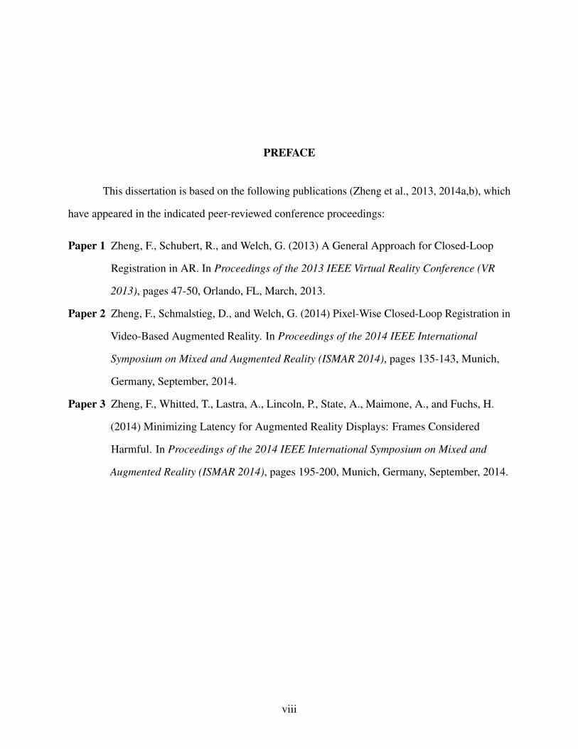
PREFACE

This dissertation is based on the following publications (Zheng et al., 2013, 2014a,b), which

have appeared in the indicated peer-reviewed conference proceedings:

Paper 1 Zheng, F., Schubert, R., and Welch, G. (2013) A General Approach for Closed-Loop

Registration in AR. In Proceedings of the 2013 IEEE Virtual Reality Conference (VR

2013), pages 47-50, Orlando, FL, March, 2013.

Paper 2 Zheng, F., Schmalstieg, D., and Welch, G. (2014) Pixel-Wise Closed-Loop Registration in

Video-Based Augmented Reality. In Proceedings of the 2014 IEEE International

Symposium on Mixed and Augmented Reality (ISMAR 2014), pages 135-143, Munich,

Germany, September, 2014.

Paper 3 Zheng, F., Whitted, T., Lastra, A., Lincoln, P., State, A., Maimone, A., and Fuchs, H.

(2014) Minimizing Latency for Augmented Reality Displays: Frames Considered

Harmful. In Proceedings of the 2014 IEEE International Symposium on Mixed and

Augmented Reality (ISMAR 2014), pages 195-200, Munich, Germany, September, 2014.

viii

TABLE OF CONTENTS

LIST OF TABLES . . . . . . . . . . . . . . . . . . . . . . . . . . . . . . . . . . . . . . . . . . . . . . . . . . . . . . . . . . . . . . . . . . . . . . . xiii

LIST OF FIGURES . . . . . . . . . . . . . . . . . . . . . . . . . . . . . . . . . . . . . . . . . . . . . . . . . . . . . . . . . . . . . . . . . . . . . . xiv

LIST OF ABBREVIATIONS . . . . . . . . . . . . . . . . . . . . . . . . . . . . . . . . . . . . . . . . . . . . . . . . . . . . . . . . . . . . . xvi

1 INTRODUCTION . . . . . . . . . . . . . . . . . . . . . . . . . . . . . . . . . . . . . . . . . . . . . . . . . . . . . . . . . . . . . . . . . . . . 1

1.1 Registration . . . . . . . . . . . . . . . . . . . . . . . . . . . . . . . . . . . . . . . . . . . . . . . . . . . . . . . . . . . . . . . . . . . . . 3

1.1.1 Registration Errors . . . . . . . . . . . . . . . . . . . . . . . . . . . . . . . . . . . . . . . . . . . . . . . . . . . . . . . 4

1.1.2 Open-Loop Registration . . . . . . . . . . . . . . . . . . . . . . . . . . . . . . . . . . . . . . . . . . . . . . . . . . 5

1.1.3 Closed-Loop Registration . . . . . . . . . . . . . . . . . . . . . . . . . . . . . . . . . . . . . . . . . . . . . . . . 5

1.2 Thesis Motivation—“The Last Mile” . . . . . . . . . . . . . . . . . . . . . . . . . . . . . . . . . . . . . . . . . . . . . 5

1.3 Thesis Statement and Contributions . . . . . . . . . . . . . . . . . . . . . . . . . . . . . . . . . . . . . . . . . . . . . . 7

1.4 Thesis Outline. . . . . . . . . . . . . . . . . . . . . . . . . . . . . . . . . . . . . . . . . . . . . . . . . . . . . . . . . . . . . . . . . . . 8

2 RELATED WORK . . . . . . . . . . . . . . . . . . . . . . . . . . . . . . . . . . . . . . . . . . . . . . . . . . . . . . . . . . . . . . . . . . . 10

2.1 Registration Errors . . . . . . . . . . . . . . . . . . . . . . . . . . . . . . . . . . . . . . . . . . . . . . . . . . . . . . . . . . . . . . 10

2.1.1 Direct Misregistration Minimization . . . . . . . . . . . . . . . . . . . . . . . . . . . . . . . . . . . . . . 11

2.1.2 Indirect Misregistration Minimization . . . . . . . . . . . . . . . . . . . . . . . . . . . . . . . . . . . . . 11

2.1.3 Discussion. . . . . . . . . . . . . . . . . . . . . . . . . . . . . . . . . . . . . . . . . . . . . . . . . . . . . . . . . . . . . . . 12

2.2 Tracking—Static Error Source . . . . . . . . . . . . . . . . . . . . . . . . . . . . . . . . . . . . . . . . . . . . . . . . . . . 12

2.2.1 Sensor-Based Tracking . . . . . . . . . . . . . . . . . . . . . . . . . . . . . . . . . . . . . . . . . . . . . . . . . . . 12

2.2.2 Vision-Based Tracking . . . . . . . . . . . . . . . . . . . . . . . . . . . . . . . . . . . . . . . . . . . . . . . . . . . 13

2.2.2.1 Marker-Based Tracking . . . . . . . . . . . . . . . . . . . . . . . . . . . . . . . . . . . . . . . . . 13

2.2.2.2 Markerless Tracking . . . . . . . . . . . . . . . . . . . . . . . . . . . . . . . . . . . . . . . . . . . . 14

ix

2.2.3 Hybrid Tracking . . . . . . . . . . . . . . . . . . . . . . . . . . . . . . . . . . . . . . . . . . . . . . . . . . . . . . . . . 17

2.2.4 Discussion. . . . . . . . . . . . . . . . . . . . . . . . . . . . . . . . . . . . . . . . . . . . . . . . . . . . . . . . . . . . . . . 18

2.3 Latency—Dynamic Error Source . . . . . . . . . . . . . . . . . . . . . . . . . . . . . . . . . . . . . . . . . . . . . . . . . 18

2.3.1 Latency Perception . . . . . . . . . . . . . . . . . . . . . . . . . . . . . . . . . . . . . . . . . . . . . . . . . . . . . . 20

2.3.2 Reducing Dynamic Errors . . . . . . . . . . . . . . . . . . . . . . . . . . . . . . . . . . . . . . . . . . . . . . . . 22

2.3.2.1 Latency Minimization . . . . . . . . . . . . . . . . . . . . . . . . . . . . . . . . . . . . . . . . . . 22

2.3.2.2 Just-In-Time Image Generation . . . . . . . . . . . . . . . . . . . . . . . . . . . . . . . . . 23

2.3.2.3 Predictive Tracking . . . . . . . . . . . . . . . . . . . . . . . . . . . . . . . . . . . . . . . . . . . . . 24

2.3.2.4 Video Feedback . . . . . . . . . . . . . . . . . . . . . . . . . . . . . . . . . . . . . . . . . . . . . . . . 26

2.3.3 Discussion. . . . . . . . . . . . . . . . . . . . . . . . . . . . . . . . . . . . . . . . . . . . . . . . . . . . . . . . . . . . . . . 26

3 CLOSED-LOOP SPATIAL REGISTRATION . . . . . . . . . . . . . . . . . . . . . . . . . . . . . . . . . . . . . . . . . . 27

3.1 Closed-Loop Projector-Based Spatial AR . . . . . . . . . . . . . . . . . . . . . . . . . . . . . . . . . . . . . . . . . 28

3.1.1 Real-Virtual Model-Based Registration . . . . . . . . . . . . . . . . . . . . . . . . . . . . . . . . . . . 28

3.1.2 Empirical Validation . . . . . . . . . . . . . . . . . . . . . . . . . . . . . . . . . . . . . . . . . . . . . . . . . . . . . 32

3.1.3 Extension to VST-AR . . . . . . . . . . . . . . . . . . . . . . . . . . . . . . . . . . . . . . . . . . . . . . . . . . . . 35

3.1.3.1 Numerical Comparison with Open-Loop Approach . . . . . . . . . . . . . . 37

3.1.4 Summary . . . . . . . . . . . . . . . . . . . . . . . . . . . . . . . . . . . . . . . . . . . . . . . . . . . . . . . . . . . . . . . . 39

3.2 Closed-Loop Video See-Trough AR . . . . . . . . . . . . . . . . . . . . . . . . . . . . . . . . . . . . . . . . . . . . . . 41

3.2.1 Global World-Space Misregistration Minimization. . . . . . . . . . . . . . . . . . . . . . . . . 43

3.2.1.1 3D Model-Based Tracking . . . . . . . . . . . . . . . . . . . . . . . . . . . . . . . . . . . . . . 43

3.2.1.2 Registration-Enforcing Model-Based Tracking . . . . . . . . . . . . . . . . . . . 45

3.2.2 Local Screen-Space Misregistration Minimization . . . . . . . . . . . . . . . . . . . . . . . . . 48

3.2.2.1 Forward-Warping Augmented Reality . . . . . . . . . . . . . . . . . . . . . . . . . . . 49

3.2.2.2 Backward-Warping Augmented Virtuality . . . . . . . . . . . . . . . . . . . . . . . 51

3.2.3 Guidelines for Global-Local Misregistration Minimization . . . . . . . . . . . . . . . . . 51

3.2.3.1 General Guidelines . . . . . . . . . . . . . . . . . . . . . . . . . . . . . . . . . . . . . . . . . . . . . 51

3.2.3.2 An Example Use . . . . . . . . . . . . . . . . . . . . . . . . . . . . . . . . . . . . . . . . . . . . . . . 53

x

3.2.3.3 Discussion . . . . . . . . . . . . . . . . . . . . . . . . . . . . . . . . . . . . . . . . . . . . . . . . . . . . . 54

3.2.4 Four-Pass Rendering . . . . . . . . . . . . . . . . . . . . . . . . . . . . . . . . . . . . . . . . . . . . . . . . . . . . . 56

3.2.4.1 Photometric Adjustments to Real Object Pixels . . . . . . . . . . . . . . . . . . 56

3.2.4.2 Photometric Adjustments to Virtual Object Pixels . . . . . . . . . . . . . . . . 58

3.2.5 Experimental Results . . . . . . . . . . . . . . . . . . . . . . . . . . . . . . . . . . . . . . . . . . . . . . . . . . . . 58

3.2.5.1 Implementation . . . . . . . . . . . . . . . . . . . . . . . . . . . . . . . . . . . . . . . . . . . . . . . . 58

3.2.5.2 Synthetic Sequences . . . . . . . . . . . . . . . . . . . . . . . . . . . . . . . . . . . . . . . . . . . . 58

3.2.5.3 Real Sequences . . . . . . . . . . . . . . . . . . . . . . . . . . . . . . . . . . . . . . . . . . . . . . . . 59

3.2.6 Limitations . . . . . . . . . . . . . . . . . . . . . . . . . . . . . . . . . . . . . . . . . . . . . . . . . . . . . . . . . . . . . . 59

3.2.7 Conclusion . . . . . . . . . . . . . . . . . . . . . . . . . . . . . . . . . . . . . . . . . . . . . . . . . . . . . . . . . . . . . . 62

3.2.8 Future Work . . . . . . . . . . . . . . . . . . . . . . . . . . . . . . . . . . . . . . . . . . . . . . . . . . . . . . . . . . . . . 63

4 LOW-LATENCY TEMPORAL REGISTRATION . . . . . . . . . . . . . . . . . . . . . . . . . . . . . . . . . . . . . . 65

4.1 Latency in Optical See-Through AR . . . . . . . . . . . . . . . . . . . . . . . . . . . . . . . . . . . . . . . . . . . . . . 65

4.2 General Approach . . . . . . . . . . . . . . . . . . . . . . . . . . . . . . . . . . . . . . . . . . . . . . . . . . . . . . . . . . . . . . . 67

4.3 The DMD as a Low-Latency Display . . . . . . . . . . . . . . . . . . . . . . . . . . . . . . . . . . . . . . . . . . . . . 69

4.3.1 DMD Chip Basics . . . . . . . . . . . . . . . . . . . . . . . . . . . . . . . . . . . . . . . . . . . . . . . . . . . . . . . 70

4.3.2 Standard DMD Projector Basics . . . . . . . . . . . . . . . . . . . . . . . . . . . . . . . . . . . . . . . . . . 70

4.3.3 Low-Latency Custom DMD Projector . . . . . . . . . . . . . . . . . . . . . . . . . . . . . . . . . . . . . 71

4.4 Experimental Results . . . . . . . . . . . . . . . . . . . . . . . . . . . . . . . . . . . . . . . . . . . . . . . . . . . . . . . . . . . . 73

4.4.1 Experiment 1: Latency . . . . . . . . . . . . . . . . . . . . . . . . . . . . . . . . . . . . . . . . . . . . . . . . . . . 74

4.4.2 Experiment 2: Low-Latency Grayscale Imagery Using Binary

Image Generation . . . . . . . . . . . . . . . . . . . . . . . . . . . . . . . . . . . . . . . . . . . . . . . . . . . . . . . . 74

4.4.3 Experiment 3: AR Imagery on Moving Object . . . . . . . . . . . . . . . . . . . . . . . . . . . . . 75

4.5 Conclusion . . . . . . . . . . . . . . . . . . . . . . . . . . . . . . . . . . . . . . . . . . . . . . . . . . . . . . . . . . . . . . . . . . . . . . 78

4.6 Future Work . . . . . . . . . . . . . . . . . . . . . . . . . . . . . . . . . . . . . . . . . . . . . . . . . . . . . . . . . . . . . . . . . . . . 78

5 FUTURE WORK . . . . . . . . . . . . . . . . . . . . . . . . . . . . . . . . . . . . . . . . . . . . . . . . . . . . . . . . . . . . . . . . . . . . . 80

5.1 Closed-Loop Optical See-Through AR . . . . . . . . . . . . . . . . . . . . . . . . . . . . . . . . . . . . . . . . . . . 80

xi

5.2 Combing Closed-Loop and Low-Latency Registration . . . . . . . . . . . . . . . . . . . . . . . . . . . . . 82

5.3 Physical-Virtual Fiducials for Closed-Loop Projector-Based Spatial AR . . . . . . . . . . . . 83

5.3.1 Error Signal Appearance . . . . . . . . . . . . . . . . . . . . . . . . . . . . . . . . . . . . . . . . . . . . . . . . . 85

5.3.2 Physical-Virtual Fiducial Design . . . . . . . . . . . . . . . . . . . . . . . . . . . . . . . . . . . . . . . . . . 85

5.3.2.1 Parameter Space . . . . . . . . . . . . . . . . . . . . . . . . . . . . . . . . . . . . . . . . . . . . . . . 86

5.3.2.2 Design Constraints . . . . . . . . . . . . . . . . . . . . . . . . . . . . . . . . . . . . . . . . . . . . . 87

5.3.2.3 Optimization Setup . . . . . . . . . . . . . . . . . . . . . . . . . . . . . . . . . . . . . . . . . . . . . 88

6 CONCLUSION. . . . . . . . . . . . . . . . . . . . . . . . . . . . . . . . . . . . . . . . . . . . . . . . . . . . . . . . . . . . . . . . . . . . . . . 89

6.1 Closed-Loop Spatial Registration . . . . . . . . . . . . . . . . . . . . . . . . . . . . . . . . . . . . . . . . . . . . . . . . 89

6.2 Low-Latency Temporal Registration . . . . . . . . . . . . . . . . . . . . . . . . . . . . . . . . . . . . . . . . . . . . . . 90

6.3 Future Possibilities . . . . . . . . . . . . . . . . . . . . . . . . . . . . . . . . . . . . . . . . . . . . . . . . . . . . . . . . . . . . . . 91

BIBLIOGRAPHY . . . . . . . . . . . . . . . . . . . . . . . . . . . . . . . . . . . . . . . . . . . . . . . . . . . . . . . . . . . . . . . . . . . . . . . . 93

xii

LIST OF TABLES

1.1 Summary of the three major AR paradigms. . . . . . . . . . . . . . . . . . . . . . . . . . . . . . . . . . . . . . . 3

3.1 Summary of mathematical notations for SAR and VST-AR. . . . . . . . . . . . . . . . . . . . . . . . 35

3.2 Analysis of all four combinations of world-space (MBT or RE-MBT) and

screen-space (FW-AR or BW-AV) misregistration minimization. . . . . . . . . . . . . . . . . . . . 52

xiii

LIST OF FIGURES

1.1 Reality–virtuality continuum . . . . . . . . . . . . . . . . . . . . . . . . . . . . . . . . . . . . . . . . . . . . . . . . . . . . . 1

1.2 Examples of different AR paradigms. . . . . . . . . . . . . . . . . . . . . . . . . . . . . . . . . . . . . . . . . . . . . . 2

1.3 Illustration of registration errors . . . . . . . . . . . . . . . . . . . . . . . . . . . . . . . . . . . . . . . . . . . . . . . . . . 4

1.4 Comparison between open-loop and closed-loop AR systems . . . . . . . . . . . . . . . . . . . . . . 6

2.1 Sample markers . . . . . . . . . . . . . . . . . . . . . . . . . . . . . . . . . . . . . . . . . . . . . . . . . . . . . . . . . . . . . . . . . 13

2.2 End-to-end system latency . . . . . . . . . . . . . . . . . . . . . . . . . . . . . . . . . . . . . . . . . . . . . . . . . . . . . . . 20

3.1 Illustration of closed-loop registration in projector-based SAR . . . . . . . . . . . . . . . . . . . . . 29

3.2 An example showing that the augmented model image Ta and the virtual

image Tv are warped using the same geometric transformation . . . . . . . . . . . . . . . . . . . . . 31

3.3 Qualitative evaluation of RV-MBR in SAR. . . . . . . . . . . . . . . . . . . . . . . . . . . . . . . . . . . . . . . . 34

3.4 Illustration of augmented image formulation in VST-AR . . . . . . . . . . . . . . . . . . . . . . . . . . 36

3.5 Qualitative evaluation of E-MBR in VST-AR and VST-DR . . . . . . . . . . . . . . . . . . . . . . . . 37

3.6 Visual registration comparison between our closed-loop approach and the

conventional open-loop approach . . . . . . . . . . . . . . . . . . . . . . . . . . . . . . . . . . . . . . . . . . . . . . . . . 38

3.7 Numerical comparison in the tracker error experiment . . . . . . . . . . . . . . . . . . . . . . . . . . . . . 39

3.8 Comparison of registration accuracy with different amounts of error in

focal length calibration . . . . . . . . . . . . . . . . . . . . . . . . . . . . . . . . . . . . . . . . . . . . . . . . . . . . . . . . . . 40

3.9 Comparison between conventional closed-loop registration and our closed-

loop registration . . . . . . . . . . . . . . . . . . . . . . . . . . . . . . . . . . . . . . . . . . . . . . . . . . . . . . . . . . . . . . . . . 42

3.10 Visualization of registration errors being iteratively minimized in VST-AR

using E-MBR . . . . . . . . . . . . . . . . . . . . . . . . . . . . . . . . . . . . . . . . . . . . . . . . . . . . . . . . . . . . . . . . . . . 46

3.11 Comparison of MBT and RE-MBT in the presence of rigid modeling errors . . . . . . . . 47

3.12 Comparison of FW-AR and BW-AV in the presence of non-rigid error sources . . . . . . 50

3.13 Input images for the specific example. . . . . . . . . . . . . . . . . . . . . . . . . . . . . . . . . . . . . . . . . . . . . 53

3.14 Illustration of the uses and differences of all four combinations of MBT

and FW-AR, MBT and BW-AV, RE-MBT and FW-AR, and RE-MBT and

BW-AV . . . . . . . . . . . . . . . . . . . . . . . . . . . . . . . . . . . . . . . . . . . . . . . . . . . . . . . . . . . . . . . . . . . . . . . . 55

xiv

3.15 Illustration of four-pass rendering . . . . . . . . . . . . . . . . . . . . . . . . . . . . . . . . . . . . . . . . . . . . . . . . 57

3.16 Comparisons between conventional open-loop registration and our closed-

loop registration using a synthetic sequence . . . . . . . . . . . . . . . . . . . . . . . . . . . . . . . . . . . . . . . 60

3.17 Comparisons between conventional open-loop registration and our closed-

loop registration using a real sequence . . . . . . . . . . . . . . . . . . . . . . . . . . . . . . . . . . . . . . . . . . . . 61

3.18 Full misregistration minimization loop . . . . . . . . . . . . . . . . . . . . . . . . . . . . . . . . . . . . . . . . . . . 63

4.1 Simulation of latency for surgery application with AR overlay (organs) . . . . . . . . . . . . 66

4.2 End-to-end low-latency AR pipeline . . . . . . . . . . . . . . . . . . . . . . . . . . . . . . . . . . . . . . . . . . . . . . 68

4.3 Experimental setup . . . . . . . . . . . . . . . . . . . . . . . . . . . . . . . . . . . . . . . . . . . . . . . . . . . . . . . . . . . . . . 73

4.4 AR registration of a moving object (pyramid) . . . . . . . . . . . . . . . . . . . . . . . . . . . . . . . . . . . . . 74

4.5 A frame of the rotating pattern projected onto a flat surface . . . . . . . . . . . . . . . . . . . . . . . . 75

4.6 Sample images used by our algorithm when displaying a rotating test

pattern with the experimental low-latency projector . . . . . . . . . . . . . . . . . . . . . . . . . . . . . . . 76

4.7 Results of the rotating cube experiment . . . . . . . . . . . . . . . . . . . . . . . . . . . . . . . . . . . . . . . . . . . 77

4.8 The rotation motion path used . . . . . . . . . . . . . . . . . . . . . . . . . . . . . . . . . . . . . . . . . . . . . . . . . . . . 77

5.1 Conceptual diagram showing using physical and virtual appearance to

achieve closed-loop registration for 2D translational motion in SAR. . . . . . . . . . . . . . . . 84

5.2 Target under different lighting directions. . . . . . . . . . . . . . . . . . . . . . . . . . . . . . . . . . . . . . . . . . 85

5.3 Parameter space for designing physical-virtual fiducials . . . . . . . . . . . . . . . . . . . . . . . . . . . 86

5.4 Optimization framework for designing physical-virtual fiducial pairs and

custom virtual fiducials . . . . . . . . . . . . . . . . . . . . . . . . . . . . . . . . . . . . . . . . . . . . . . . . . . . . . . . . . . 88

xv

LIST OF ABBREVIATIONS

AR Augmented Reality

AV Augmented Virtuality

BW-AV Backward-Warping Augmented Virtuality

DLP Digital Micromirror Processing

DMD Digital Micromirror Device

DOF Degree of Freedom

DR Diminished Reality

EKF Extended Kalman Filter

E-MBR Extended Model-Based Registration

FW-AR Forward-Warping Augmented Reality

GPU Graphics Processing Unit

HWD Head-Worn Display

KF Kalman Filter

MR Mixed Reality

MBT Model-Based Tracking

OF Optical Flow

OST-AR Optical See-Through Augmented Reality

ProCam Projector-Camera

RE-MBT Registration-Enforcing Model-Based Tracking

RV-MBR Real-Virtual Model-Based Registration

SAR Spatial Augmented Reality

V-Sync Vertical Synchronization

VE Virtual Environment

VR Virtual Reality

VST-AR Video See-Through Augmented Reality

xvi

CHAPTER 1: INTRODUCTION

Augmented Reality (AR) combines computer-generated virtual imagery with the user’s live

view of the real environment in real time, enhancing the user’s perception of and interaction with

the real world. According to Azuma et al. (2001), an AR system comprises the following properties:

• combines real and virtual objects in a real environment;

• runs interactively, and in real time; and

• registers (aligns) real and virtual objects with each other.

The reality–virtuality continuum (Milgram et al., 1995), as shown in Figure 1.1, is a

notional scale that extends from the completely real (reality) to the completely virtual (virtuality).

AR is one part of the general area of Mixed Reality (MR). Unlike Virtual Reality (VR) (also known

as Virtual Environment or VE), where the user is completely immersed in a virtual environment,

AR allows the user to see the real world and interact with virtual objects using real objects (e.g.,

user’s hand) in a seamless way.

Real Environment

Augmented Reality (AR)

Augmented Virtuality (AV)

Virtual Environment

Mixed Reality (MR)

Figure 1.1: Reality–virtuality continuum.

A basic AR system consists of three components: (1) a tracking subsystem, which

dynamically measures six degrees of freedom (DOF) pose of the viewpoint (3DOF for position and

the other 3DOF for orientation), (2) a rendering subsystem, which draws virtual objects based on

tracking input, and (3) a display subsystem, which displays the rendering output. Depending on

1

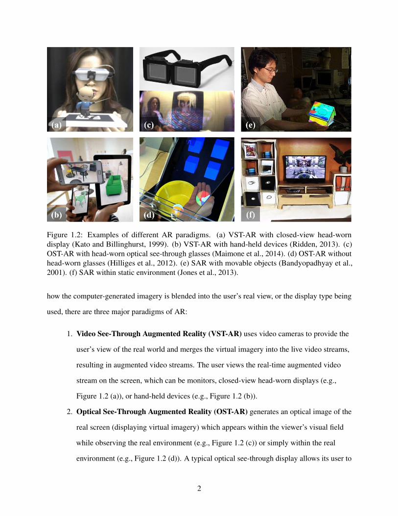
Figure 1.2: Examples of different AR paradigms. (a) VST-AR with closed-view head-worn

display (Kato and Billinghurst, 1999). (b) VST-AR with hand-held devices (Ridden, 2013). (c)

OST-AR with head-worn optical see-through glasses (Maimone et al., 2014). (d) OST-AR without

head-worn glasses (Hilliges et al., 2012). (e) SAR with movable objects (Bandyopadhyay et al.,

2001). (f) SAR within static environment (Jones et al., 2013).

how the computer-generated imagery is blended into the user’s real view, or the display type being

used, there are three major paradigms of AR:

1. Video See-Through Augmented Reality (VST-AR) uses video cameras to provide the

user’s view of the real world and merges the virtual imagery into the live video streams,

resulting in augmented video streams. The user views the real-time augmented video

stream on the screen, which can be monitors, closed-view head-worn displays (e.g.,

Figure 1.2 (a)), or hand-held devices (e.g., Figure 1.2 (b)).

2. Optical See-Through Augmented Reality (OST-AR) generates an optical image of the

real screen (displaying virtual imagery) which appears within the viewer’s visual field

while observing the real environment (e.g., Figure 1.2 (c)) or simply within the real

environment (e.g., Figure 1.2 (d)). A typical optical see-through display allows its user to

2

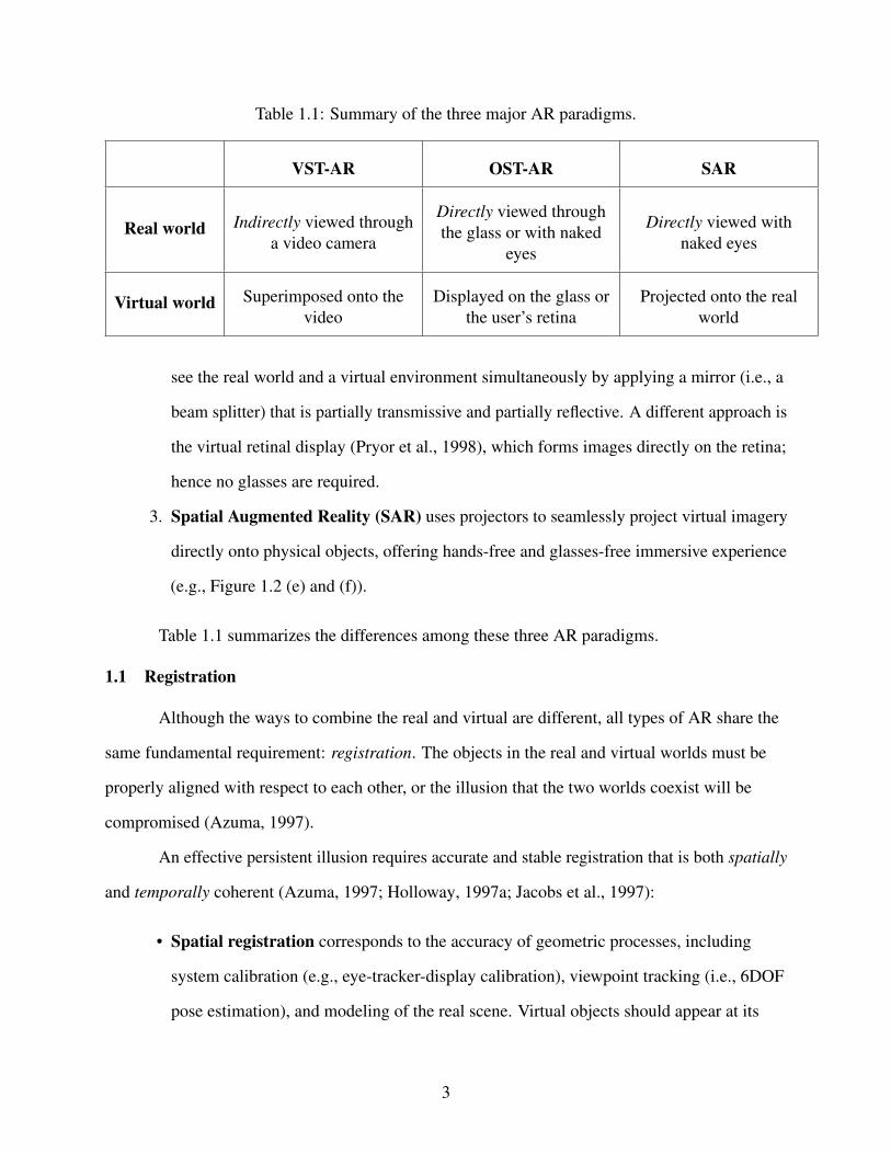
Table 1.1: Summary of the three major AR paradigms.

VST-AR OST-AR SAR

Real world Indirectly viewed through

a video camera

Directly viewed through

the glass or with naked

eyes

Directly viewed with

naked eyes

Virtual world Superimposed onto the

video

Displayed on the glass or

the user’s retina

Projected onto the real

world

see the real world and a virtual environment simultaneously by applying a mirror (i.e., a

beam splitter) that is partially transmissive and partially reflective. A different approach is

the virtual retinal display (Pryor et al., 1998), which forms images directly on the retina;

hence no glasses are required.

3. Spatial Augmented Reality (SAR) uses projectors to seamlessly project virtual imagery

directly onto physical objects, offering hands-free and glasses-free immersive experience

(e.g., Figure 1.2 (e) and (f)).

Table 1.1 summarizes the differences among these three AR paradigms.

1.1 Registration

Although the ways to combine the real and virtual are different, all types of AR share the

same fundamental requirement: registration. The objects in the real and virtual worlds must be

properly aligned with respect to each other, or the illusion that the two worlds coexist will be

compromised (Azuma, 1997).

An effective persistent illusion requires accurate and stable registration that is both spatially

and temporally coherent (Azuma, 1997; Holloway, 1997a; Jacobs et al., 1997):

• Spatial registration corresponds to the accuracy of geometric processes, including

system calibration (e.g., eye-tracker-display calibration), viewpoint tracking (i.e., 6DOF

pose estimation), and modeling of the real scene. Virtual objects should appear at its

3

proper location in the real world with proper real-virtual occlusions, otherwise the user

cannot correctly determine spatial relationships.

• Temporal registration corresponds to synchronized motion between the real and virtual

over time. Virtual objects should be updated and redisplayed at the same time as

corresponding updates and changes in the physical-world scene. End-to-end system

latency (also known as motion-to-photon latency) is directly related to temporal

misregistration. It is defined as the time difference between the moment that the object or

the viewpoint moves to the moment that the updated virtual image corresponding to the

motion appears in the display.

1.1.1 Registration Errors

Visible registration errors are present in most AR systems. They are perceived by the user

in the final augmented imagery as misalignment between the real and virtual objects. Registration

errors can be divided into three categories (Holloway, 1997a): (1) linear registration error, (2)

lateral registration error, and (3) depth registration error. An illustration is shown in Figure 1.3.

Figure 1.3: Illustration of registration errors. Source: Daponte et al. (2014).

There are numerous sources of error that can result in visible misregistration. These sources

of error can be divided into two types: dynamic and static. Dynamic errors are errors arising from

various system delays, which have no effect until the user’s viewpoint or the object begins moving.

4

Static errors are constant errors arising from geometric processes (calibration, tracking, and

modeling), that cause registration errors even when there is no relative motion between the

viewpoint and the object to be augmented. One can say that dynamic error sources cause temporal

misregistration, while static error sources cause spatial misregistration. See Holloway (1997a) for a

comprehensive analysis of error sources and magnitudes of misregistration.

1.1.2 Open-Loop Registration

The conventional method for achieving registration is a four-step process in which

independent mechanisms are used first to do an one-time calibration of system parameters, then to

dynamically track the object to be augmented, to render the appropriate virtual content to be

overlaid on the real object using the tracking data, and finally to display the result. This is

analogous to an open-loop system, shown in Figure 1.4 (a). Such an open-loop system has no

mechanism for observing registration errors—it simply generates the virtual content that should be

consistent with the geometric process, assuming there are no errors. The only way to improve such

system is to make each system component more accurate. However, no matter how carefully we

perform the geometric process, we cannot eliminate all errors.

1.1.3 Closed-Loop Registration

Conversely closed-loop AR systems sense their own output (i.e., augmented imagery to be

observed by the user), and attempt to minimize any detected errors, as shown in Figure 1.4 (b).

Such systems can automatically and continuously adjust system parameters in space and time to

maintain the desired augmented appearance.

1.2 Thesis Motivation—“The Last Mile”

The overarching goal of AR is to provide users with the illusion that virtual and real objects

coexist in the same space. Enabling technologies needed to build compelling AR environments,

such as tracking, interaction and display, have come a long way over the years (Zhou et al., 2008).

Over the past two decades, many researchers have demonstrated the promise of AR, allowing

society to reach new levels of capability and efficiency in areas as diverse as medicine (Fuchs et al.,

5

(a) Open-loop AR system

(b) Closed-loop AR system

Figure 1.4: Comparison between open-loop and closed-loop AR systems.

1998), manufacturing (Caudell and Mizell, 1992), maintenance (Feiner et al., 1993),

navigation (Feiner et al., 1997), and telepresence (Neumann and Fuchs, 1993). To date, however,

AR has been primarily confined to the lab, mainly due to huge challenges involved in achieving

“the last mile” 1 of registration. “The last mile” refers to the final delivery of accurately registered

augmented imagery to the end user, free of perceivable errors. However, registration errors are

difficult to adequately control because of the high accuracy requirements and the numerous sources

of error (Azuma, 1997).

Among all error sources, system latency is the largest single source of registration error in

existing AR systems, outweighing all others combined (Holloway, 1997a). Latency results in

temporal misregistration, manifested as virtual imagery lagging behind or “swimming” around the

intended position. All AR systems suffer from the unavoidable delay between sampling a sensor

and modifying the display. Every action pertaining to the registration, e.g., tracking, rendering, and

display, requires some amount of time to occur. Unfortunately, todays hardware (GPUs) and

1 The term “the last mile” has its origin in telecommunications and supply chain management. It describes the last

segment in a communication or distribution network that actually reaches the customer. Such end link between

consumers and connectivity has proved to be disproportionately expensive to solve.

6

software (drivers and graphics APIs) are not designed for minimal latency but rather for highest

possible throughput, which they achieve through a combination of parallelism and pipelining. Even

as it increased frame rates, it has been a source of increased latency. Predictive tracking is a good

workaround for short delays, but it does not allow us to relax the restraint that the system operates

with quick turnaround (Azuma, 1995). Therefore, we must minimize latencies in all system

components all the way from motion sensing to photon display, if possible.

Other most serious error sources are in the geometric processes, especially 6DOF pose

tracking. An AR system needs to know the geometric relationship between the user’s eyes, the

display(s) and the objects in the world. Inaccurate geometric processes result in spatial

misregistration, usually manifested as virtual imagery (1) offset constantly, due to calibration or

modeling errors; (2) jittery, due to unstable tracking; or (3) drift-away, due to error accumulation.

However, most AR systems are open-loop. The result is that inaccurate geometric processes lead to

misregistration that is seen by the users but not the system. Careful measurement of these

geometric relationship will reduce some of these registration errors, but they can never be

completely eliminated in any realistic system (MacIntyre and Julier, 2002). Therefore, we must

“close the loop” by feeding the output registration back into the system and have the system

automatically minimize any visible errors.

1.3 Thesis Statement and Contributions

This thesis is motivated by “the last mile” of registration in AR—the final imagery observed

by the user should be free of perceivable errors. “This last mile” demands AR systems to be

low-latency and closed-loop.

Thesis Statement

Closed-loop real-virtual spatial adaptation and low-latency fine-grained render-display

processing can be used to achieve optimal visual registration in Augmented Reality systems.

The main contributions of this dissertation can be summarized as follows:

7

1. I present real-virtual model-based registration (RV-MBR) as an effective closed-loop

registration method, which continuously adjusts geometric transformation parameters to

maintain the desired augmented appearance in projector-based SAR. It does so without

the explicit detection and use of features or points in the camera imagery, instead

optimizing the parameters directly using any misregistration manifested in the augmented

imagery.

2. I introduce registration-enforcing model-based tracking (RE-MBT) as a new paradigm for

registration in VST-AR, offering a valuable extension to existing AR approaches relying

on conventional model-based tracking (MBT). RE-MBT is capable of refining the camera

poses towards better registration by selective weighting of important image regions, even

in the presence of modeling errors.

3. I show how real-time optical flow can be used in a post-process in VST-AR to minimize

residual registration errors in image space, even in the presence of non-rigid errors. I

introduce two alternative ways of using (feeding back) the optical flow: forward warping

Augmented Reality (FW-AR) and backward warping Augmented Virtuality (BW-AV).

The latter uses the camera image to re-texture the rendered real scene model.

4. I propose a low-latency image generation algorithm, reducing latency to the minimum in

DLP™ DMD projectors, which are widely used in OST-AR. Grayscale display can be

achieved via binary adjustments at the maximum binary rate. The resulting displayed

binary image is “neither here nor there,” but always approaches the moving target that is

constantly changing desired image, even when that image changes every 50 µs.

1.4 Thesis Outline

The rest of the dissertation is organized as follows. Chapter 2 describes related work in the

areas of misregistration minimization, tracking, and latency. Chapter 3 proposes methods for

closed-loop spatial registration in SAR and VST-AR. For VST-AR, I propose a global-local

misregistration minimization method that can deal with both rigid and nonrigid errors and obtain

pixel-accurate registration. Chapter 4 presents a general end-to-end system pipeline with low

8

latency, and an algorithm for minimizing latency in displays (DLP™ DMD projectors in particular).

Chapter 5 discusses future steps that may further improve spatio-temporal registration. Particularly,

I discuss possibilities for designing custom virtual or physical-virtual fiducials for closed-loop

registration in SAR. Finally, Chapter 6 summarizes the results, contributions and future possibilities

of the dissertation.

9

CHAPTER 2: RELATED WORK

This chapter describes previous work in spatio-temporal registration in AR, beginning with

a review of misregistration minimization techniques in Section 2.1. This is followed by a discussion

of tracking techniques in AR in Section 2.2, as tracking is the most serious source of static

misregistration. Finally, Section 2.3 introduces related work on latency, which is the dynamic error

source.

2.1 Registration Errors

If computer-generated imagery is poorly aligned with the real world, it can be confusing,

annoying, misleading, or even dangerous for applications such as AR-assisted surgery (Fuchs et al.,

1998). The challenges of accurate registration are significant for Video See-Through AR (VST-AR)

and projector-based Spatial AR (SAR) systems (e.g, Dedual et al. (2011); Kato and Billinghurst

(1999); Bimber and Raskar (2005)) and even more so for Optical See-Through AR (OST-AR)

systems (e.g, Menozzi et al. (2014); Sutherland (1968)). Holloway (1997a) conducted a

comprehensive analysis of registration errors and summarized a number of important error sources

in OST-AR with head-worn displays, including calibration error, tracking error, system delay, and

misalignment of the model. VST-AR and SAR systems suffer from the same major error sources.

The principal difference of VST-AR in comparison with SAR and OST-AR is that in VST-AR, the

video stream can be deliberately delayed or otherwise modified to match the virtual image in space

and time (Bajura and Neumann, 1995).

All AR systems must deal with registration errors. There is much existing work attempting

to minimize registration errors, either directly or indirectly.

10

2.1.1 Direct Misregistration Minimization

Some previous work has attempted to obtain pixel-wise registration adjustments for

accurate occlusion between the real and virtual objects. Klein and Drummond (2004) identify

boundaries and edges where the real world occludes the virtual imagery and then use the error to

adapt polygonal phantom geometry for better real-virtual occlusion. Similarly, DiVerdi and

Hollerer (2006) use edge searching in a pixel shader to obtain per-pixel occlusion correction,

however, they adapt polygon boundaries in screen space rather than adjusting the pose estimate for

the entire polygon.

2.1.2 Indirect Misregistration Minimization

Some research tries to work around the registration errors by using pre-registered

augmented images or by attempting to mitigate the consequences of misregistration. The former is

exemplified by Indirect AR (Wither et al., 2011), which displays previously acquired panoramas of

a scene with carefully registered augmentations, rather than capturing and displaying live images.

Similarly, Quarles et al. (2010) allows the user to see a virtual version of the real world around

them on their hand-held screen that is roughly registered to the world, but they show only a portion

of the scene rather than a complete annotated panoramic image of the world around them. Such

indirect methods avoid tracking errors with traditional AR registration and can enable perfect

alignment of virtual content, but they only work for VST-AR.

The latter is demonstrated by MacIntyre and M. Coelho (2000), who introduce level of

error (LOE) rendering to adapt virtual content in order to camouflage registration errors caused by

tracking inaccuracies (based on the manufacturer-reported error range). As a follow-up, MacIntyre

and Julier (2002) improve registration error estimation with a statistical method which models

errors as probability distributions over the input values to the coordinate system transformations.

This method accounts for errors in both tracking and head-worn display calibration, but not

temporal errors. Robertson and MacIntyre (2004) enhance LOE by leveraging semantic knowledge

to further ameliorate the effects of registration errors. They introduce a set of AR visualization

techniques for creating augmentations that contain sufficient visual context for a user to understand

11

the intent of the augmentation, which are demonstrated to be effective in a user study (Robertson

et al., 2009).

2.1.3 Discussion

In contrast to previous work, our proposed closed-loop registration approach minimizes

registration errors in both global world space via camera pose refinement and local screen space via

pixel-wise corrections, to handle a larger variety of non-rigid registration errors. All of our global

world-space misregistration minimization methods (RV-MBR, E-MBR, MBT, and RE-MBT)

directly minimize errors in tracking. For local screen-space misregistration minimization methods,

FW-AR directly minimizes registration errors in real camera space, while BW-AV can be

considered as an indirect method as it minimizes misregistration by warping the real camera image

into the virtual camera space.

2.2 Tracking—Static Error Source

The real-time estimation of eye/camera position and orientation (6DOF pose), also known

as “tracking,” has long been considered one of the most crucial aspects of AR (Azuma, 1997). It is

so important because for most applications, the perceived quality of an AR display is a direct

function of tracking accuracy. Unfortunately, tracking is the most serious source of static errors;

even small tracking errors will result in visible registration errors.

In 1968, Ivan Sutherland stated the goal was a resolution of 1/100 of an inch and one part in

10,000 of rotation (Sutherland, 1968). Some of today’s systems claim to achieve position accuracy

and resolution of tenths of millimeters, and orientation accuracy and resolution of hundredths of

degrees, all with latencies on the order of milliseconds. They do so using a variety of modalities

(e.g., magnetic fields, acoustic waves, inertia, and light) in a variety of configurations. In general,

we can classify them into three categories: sensor-based, vision-based, and hybrid tracking.

2.2.1 Sensor-Based Tracking

Sensor-based tracking techniques are based on sensors such as magnetic, acoustic, inertial,

optical, and mechanical sensors. They are typically robust and fast but less accurate than

12

(a) ARToolKit marker (b) ARTag marker (c) Multi-ring marker (d) Random dot marker

Figure 2.1: Sample markers. (a) ARToolKit marker (Kato and Billinghurst, 1999). (b) ARTag

marker (Fiala, 2010). (c) Multi-ring marker (Y. Cho and Neumann, 1998). (d) Random dot

marker (Uchiyama and Saito, 2011).

vision-based tracking. Sensor-based tracking has been well developed as part of Virtual Reality

research. See (Meyer et al., 1992; Bhatnagar, 1993; Rolland et al., 2001; Allen et al., 2001; Welch,

2009) for relatively comprehensive overviews.

2.2.2 Vision-Based Tracking

Arguably the most prevalent approach for tracking in AR is to use computer vision.

Vision-based methods offer the advantage that they typically estimate the pose by observing

features in the environment near the desired location of the augmentation. The low cost of video

cameras and the increasing availability of video capture capabilities in off-the-shelf PCs and mobile

devices have inspired substantial research into the use of video cameras as sensors for tracking.

2.2.2.1 Marker-Based Tracking

Marker-based tracking uses fiducial markers (artificial landmarks), which are placed in the

scene to facilitate locating point correspondences between images, or between an image and a

known model. The most famous marker-based tracking approach is ARToolKit (Kato and

Billinghurst, 1999), which uses a heavy black square frame within which a unique pattern is printed.

Rudimentary image processing can be used for marker detection: image thresholding, line finding,

and extracting regions bounded by four straight lines. Each marker, having four corners, yields a

full 3D pose. Numerous enhancements have been made over ARToolKit, including less

inter-marker confusion (Fiala, 2005, 2010), more stable pose estimation (Wagner and Schmalstieg,

13

2007), less visual clutter (Wagner et al., 2008a), and robustness to noise (Owen et al., 2002),

occlusion (Olson, 2011), and motion blur (Herout et al., 2013). Other researchers explore tracking

using non-square markers, such as ring-shaped (Y. Cho and Neumann, 1998), circular 2D

bar-coded (Naimark and Foxlin, 2002), or even randomly scattered dots (Uchiyama and Saito,

2011). Several sample markers are shown in Figure 2.1.

Because of its reliability and efficiency as well as the availability of many open-source

libraries, maker-based tracking is widely used for rapid AR application development. While using

markers can simplify the 3D tracking task, its main drawback is the requirement of manual

engineering of the environment, which makes it limited to indoor use.

2.2.2.2 Markerless Tracking

Rather than using fiducial markers, markerless tracking relies on natural information

present in the camera image, such as points, edges, or image intensities.

Feature-Based Tracking

Feature-based tracking methods track local features such as line segments, edges, or

contours across a sequence of images. These techniques are generally robust to lighting change and

occlusions, but sensitive to feature detection and they cannot be applied to complex images that do

not naturally contain special sets of features to track. Feature-based tracking can be further

classified, according to the type of feature used, into edge-based and point-based.

Edge-based tracking. Edges correspond to discontinuities in image intensities. They are

relatively robust to lighting changes and easy to extract from images. Historically, the early

approaches to tracking were all edge-based, mostly because these methods are both

computationally efficient, and relatively easy to implement (Lepetit and Fua, 2005). Because of its

low computational complexity, the RAPiD (Real-time Attitude and Position Determination)

approach (Harris and Stennett, 1990) was one of the first markerless 3D trackers to successfully run

in real time. For every frame, RAPiD performs the following: (1) render a CAD model of object

edges according to the latest predicted pose, (2) measure the image-space difference between

14

predicted and actual edge locations by small, one-dimensional edge searches performed from

control points on the CAD model edges, and (3) update 6DOF pose to minimize the difference by

linearizing about the current pose estimate, differentiating each edge distance with respect to the six

pose parameters and solving for a least-squares solution. Increases in processing power and

advances in technique have since given rise to many systems which take the basic ideas of RAPiD

to the next level (Armstrong and Zisserman, 1995; Drummond and Cipolla, 2002; Seo et al., 2014).

Edge-based tracking methods are generally accurate for estimating small pose changes, but they

cannot cope with sudden large camera motions. Therefore, previous AR systems usually combine

them with sensor-based tracking to handle a wide variety of motions. Such hybrid approaches are

further discussed in Section 2.2.3.

Keypoint-based tracking. Keypoint features, or interest points, e.g., harris corner (Harris

and Stephens, 1988), SIFT (Lowe, 2004), or Ferns (Ozuysal et al., 2007), are discriminative image

points, usually described by the appearance of patches of pixels surrounding the point location. One

of the first AR systems using keypoint-based tracking was done by Park et al. (1999), using natural

image points to extend the range and robustness of marker-based tracking. Without the use of any

fiducials for initialization, Simon et al. (2000) require the user to manually indicate the planar

region in the first frame and then track the planar region continuously. Keypoints are detected in

each frame and matched to those detected in the previous frame in order to compute the inter-frame

homography, from which the 6DOF pose can be extracted. Wagner et al. (2008b) present the first

real-time 6DOF keypoint-based tracking system for mobile phones, which heavily modifies SIFT to

be less computationally expensive and Ferns to be less memory intensive.

Intensity-Based Tracking

Intensity-based tracking methods estimate the movement, the deformation, or the

illumination parameters of a reference template between two frames by minimizing an error

measure based on image intensities. Many these techniques are extended from the seminal work

of Lucas and Kanade (1981), which was originally proposed for 2D image alignment with sub-pixel

precision but can be generalized to register a 2D template to an image under a family of

15

transformations, such as affine, homography, and rigid-body 6DOF transformation. Baker and

Matthews (2004) present a unifying framework to understand and categorize many variants of the

Lucas-Kanade (LK) method. One of the notable variants is the Inverse Compositional (IC)

algorithm (Baker and Matthews, 2001), which is as accurate as the LK method but more efficient by

making the Hessian matrix constant so that it can be precomputed. Benhimane and Malis (2004,

2007) further improve IC by using efficient second-order minimization (ESM), which achieves a

better convergence rate without a loss of accuracy or efficiency.

With intensity-based tracking, the template can be 2D images or 3D textured models. In the

case of 2D templates, these methods are also known as template-based tracking (Baker and

Matthews, 2001; Benhimane and Malis, 2004, 2007; Lieberknecht et al., 2009). In the case of 3D

templates, these methods are also known as 3D model-based tracking (MBT) or

tracking-by-synthesis (Li et al., 1993; Reitmayr and Drummond, 2006; Simon, 2011). Reitmayr

and Drummond (2006) use tracking-by-synthesis in AR by rendering a textured model of the real

environment for subsequent feature matching with the live video image. While this approach is

sparse and intended for pose tracking, it could be used to implement closed-loop tracking in the

context of this thesis as well (Section 3.2).

Simultaneous Tracking and Mapping

Simultaneous Localization and Mapping (SLAM) refers to a set of methods to solve the

pose estimation and 3D reconstruction problem simultaneously while a system is moving through

the environment. SLAM has received great interest in the AR community in recent years. Initial

work by Davison et al. (2003) demonstrated that a real-time SLAM method for AR, using a single

color camera, is able to build a 3D model of its environment while also tracking the camera pose.

This method is accurate and fast for tracking a handheld or wearable camera in an unknown

environment, but the reconstructed model is very sparse. PTAM (Parallel Tracking and Mapping)

by Klein and Murray (2007) demonstrates superior robustness and the ability to create models with

thousands of 3D points by splitting tracking and mapping into two CPU threads. DTAM (Dense

Tracking and Mapping) by Newcombe et al. (2011a) brings real-time monocular SLAM to a new

16

level, not only tracking a freely-moving color camera but also performing dense reconstruction of

the static scene (producing a surface patchwork with millions of vertices) using powerful

commodity GPGPU hardware.

With the introduction of low-cost depth sensors, such as the Microsoft Kinect, RGB-D

SLAM methods have become popular in AR (Newcombe et al., 2011b; Meilland et al., 2013;

Salas-Moreno et al., 2013, 2014). The most representative work is KinectFusion (Newcombe et al.,

2011b), which demonstrates a live dense tracking and reconstruction system with better accuracy

and robustness than any previous solution using passive computer vision.

Visual Servoing

Visual servo control refers to the use of computer vision data to control the motion of a

robot, relying on techniques from image processing, computer vision, and control

theory (Chaumette and Hutchinson, 2006, 2007). Our closed-loop approach has its roots in

conventional control theory. It is related to virtual visual servoing (Comport et al., 2006), whose

task is to control the virtual camera using estimated pose to match the real camera for AR

registration. Benhimane and Malis (2007) have theoretically proved the existence of the

isomorphism between the task function and the camera pose and the local stability of the control

law for homography-based 2D visual servoing.

2.2.3 Hybrid Tracking

Vision-based tracking performs best with low frequency motion but is prone to failure given

rapid movements, such as head motion. Sensor-based tracking is better suited for measuring

high-frequency, rapid motion but is susceptible to noise and bias drift with slow movement. The

complementary nature of vision-based and sensor-based tracking leads to hybrid tracking, which

combines the strength of both methods. Azuma et al. (1999) describes the necessity of hybrid

tracking in order to make AR work outdoors. You et al. (1999) combine inertial (gyroscope and

accelerometer) tracking and vision-based tracking to produce nearly pixel-accurate results on

known landmark features in outdoor scenes. Klein and Drummond (2003) combine an edge-based

17

tracker, RAPiD (Harris and Stennett, 1990), which is accurate for small motions, with rate

gyroscopes, which are robust to rapid rotations. Recent work by Oskiper et al. (2011) demonstrates

a highly-accurate and stable hybrid tracking method for both indoor and outdoor AR over large

areas. This approach uses an error-state Extended Kalman Filter (EKF) to fuse Inertial

Measurement Unit (IMU) output, visual odometry based relative pose measurements, and global

pose measurements as a result of landmark matching through a pre-built visual landmark database.

2.2.4 Discussion

While we are fortunate to have access to such relatively robust and accurate approaches, as

indicated earlier, even the best system/approach cannot ensure accurate real-virtual registration

alone, as such systems do not observe or correct the registration in the final augmented image.

Errors caused by (for example) manufacturing inaccuracies, signal delays, and dynamic variations

in components and parameters conspire against registration. This is compounded by errors in the

models for the objects/scenes we are trying to augment. These inevitable errors and perturbations

are magnified by distance and other factors, and manifest themselves as misregistered and unstable

imagery. This is the motivation for our closed-loop approach, which can be implemented using

virtually any tracking system suited to a specific situation, combined with our global-local

misregistration minimization.

2.3 Latency—Dynamic Error Source

Latency results in temporal misregistration, manifested as virtual imagery lagging behind or

“swimming” around the intended position. It is the single largest source of registration error in

existing AR systems, outweighing all other error sources combined (Holloway, 1997a). End-to-end

system latency is the sum of delays from tracking, application, rendering, scanout, display, and

synchronization among components (Jerald, 2009):

• Tracking delay is the time from when the user or the object moves until motion

information from the tracker’s sensors resulting from that movement is input into the

application or rendering component of the system. If tracking is processed on a different

18

computer from the computer that executes the application and rendering, tracking delay

includes the network delay

• Application delay is time due to computation other than tracking or rendering, e.g.,

updating the world model, user interaction, and physics simulation. It can vary greatly

depending on the complexity of the task and the virtual world.

• Rendering delay is the time from when new data enters the graphics pipeline to the time

an image resulting from that data is completely drawn into a buffer (framebuffer). It

depends on the complexity of the virtual world, the desired quality of the resulting image,

and the performance of the graphics software/hardware.

• Scanout delay is the time from when a pixel is drawn into the framebuffer to the time

that pixel is transferred to the display device. Common display interfaces (e.g., VGA,

DVI, and HDMI) use raster scan method, which scanning pixels out from the GPU to the

display left-to-right in a series of horizontal scanlines from top to bottom (Whitton, 1984).

• Display delay is the time from when a pixel arrives at the display device to the time that

pixel’s light reaches users’ eyes. It depends on the technology of the display hardware

(e.g., LCD, DLP, and OLED (Wikipedia, 2015a)).

• Synchronization delay is the delay that occurs due to integration of pipelined

components. It can be due to components waiting for a signal to start new computations

and/or can be due to asynchrony among components. For example, V-Sync (Vertical

Synchronization) is used to synchronize the GPU and display to the vertical blanking

interval, where the GPU sends rendered frames to the display on a fixed cadence (60

times per second for a 60 Hz display).

Figure 2.2 shows how these delays contribute to total system latency. As noted by Jerald

(2009), system latency can be greater than the inverse of the update rate, i.e., a pipelined system can

have a frame rate of 60 Hz but have a delay of several frames, e.g., due to additional internal

buffering. See (Welch and Davis, 2008) for a more extensive analysis of tracking and

19

Tracking Delay

Application Delay

Rendering Delay

Scanout Delay

Display Delay

Synchronization Delay

The System

The User

Figure 2.2: End-to-end system latency comes from the delay of the individual systems components

and from the synchronization of those components [adapted from (Jerald, 2009)].

synchronization delays, and (Ohl et al., 2015) for detailed latency analysis in telepresence systems

with distributed acquisition and rendering.

2.3.1 Latency Perception

Researchers have identified the need for minimal total system latency in both VR and AR

applications (Olano et al., 1995; NVIDIA, 2013). To avoid certain deleterious effects of VR (such

as what is commonly known as “simulator sickness”), it is desirable to keep system response to

head motion roughly as fast or faster than the vestibuloocular reflex, one of the fastest reflexes in

the human body at 7ms to 15ms (Amin et al., 2012). This reflex rapidly stabilizes the retinal image

at the current fixation point by rotating the eye in response to head motion. For example, the

developers of the Oculus VR headset recommend “20ms or less motion-to-photon latency” (Yao

et al., 2014). To help developers reach that goal, they have recently reduced the latency of the

Oculus Rift tracking subsystem to 2ms (Luckey, 2013). Various experiments conducted at NASA

Ames Research Center conclude that the Just Noticeable Difference (JND) for latency

20

discrimination is in the 5 to 20ms range (Adelstein et al., 2003; Ellis et al., 2004; Mania et al.,

2004), independent of scene complexity and real-world meaning (Mania et al., 2004). Even smaller

total latencies are recommended when a VR experience conveying a high sensation of presence is

needed: to avoid any perception of scene motion due to latency, values as low as 3ms should not be

exceeded (Jerald and Whitton, 2009; Jerald, 2009). A NASA study investigating the utility of

head-worn displays for flight deck “Synthetic/Enhanced Vision Systems” concludes that

commonplace “head movements of more than 100 °/s would require less than 2.5ms system latency

to remain within the allowable [Heads-Up Display] error levels” (Bailey et al., 2004).

Touch-based interaction with displays also represents a form of AR, in that the user should

ideally perceive display elements as being affected by touch as if they were tangible objects (e.g.

when dragging). Previous work in this related area covers both user perception and task

performance; the conclusions include that “there is a perceptual floor somewhere between 2−11ms,

below which users do not notice lag” and that “latencies down to 2.38ms are required to alleviate

user perception when dragging” (Jota et al., 2013; Ng et al., 2012).

There are numerous results on the effect of latency in the literature. For example, the JND

for latency discrimination is shown to be dependent on the speed of head movement using a

HWD (Allison et al., 2001). Considering physiological measurements, Meehan et al. (2003) find

that with a lower latency of 50 ms there is more physiological reaction to a virtual stress provoking

environment than with a latency of 90 ms. Samaraweera et al. (2013) show that mobility impaired

persons react to latency and the presence of an avatar differently than healthy users and avatars may

have an effect on gait but only at higher latencies. The effect of latency in collaborative VEs is task

dependent—the more precision is needed the less latency is tolerated (Park and Kenyon, 1999). In

addition, jitter—the variation of the latency—is in general more harmful than latency (Park and

Kenyon, 1999; Vaghi et al., 1999).

21

2.3.2 Reducing Dynamic Errors

There are four approaches to reducing dynamic registration errors caused by latency:

latency minimization, just-in-time image generation, predictive tracking, and video

feedback (Holloway, 1997b; Azuma, 1997).

2.3.2.1 Latency Minimization

This is the most straightforward approach, which aims at directly reducing latencies in

system components and making them more responsive. Olano et al. (1995) minimize latency in

rendering by reconfiguring the conventional pipeline at the cost of throughput. Their low-latency

rendering system reduces image generation time from 50-75 ms to 17 ms. Regan et al. (1999) build

a low-latency hardware system for VR consisting of a low-latency mechanical-arm tracker and a

low-latency light-field renderer by deliberately over engineering for latency minimization. SCAAT

(Single-Constraint-At-A-Time) reduces tracking latency by producing pose estimates as each new

low-level sensor measurement is made rather than waiting to form a complete collection of

observations (Welch and Bishop, 1997). Stichling et al. (2006) extend synchronous dataflow graphs

with linear processing and fine-grained pipelining for vision-based feature tracking to reduce

latency and minimize storage for mobile devices.

As noted by Wloka (1995), being careful about synchronizing pipeline tasks can also

reduce end-to-end system latencies. Harders et al. (2009) achieve temporal synchronization of two

distributed machines (a graphics client and a physics server) in a visuo-haptic AR application by

transmitting network packets between the machines, in which system clock times are stored. Hill

et al. (2004) synchronize the tracker readings with the V-Sync signal to eliminate the dynamic

asynchrony, which results from the absence of synchronization between the tracker device readings

and the updates of the graphics application. To deal with the synchronization delay that occurs

between the buffer swapping and the V-Sync signal, Hill et al. (2004) connect the V-Sync signal

from the VGA output of the graphics card to the parallel port of the computer and having the VE

application poll the port using the UserPort kernel driver. In (Papadakis et al., 2011), triple buffering

and V-Sync are disabled from the control panel of the graphics card, which lead to the reduction of

22

the overall latency due to dynamic asynchrony, but introduce image tearing. Recently, NVIDIA

(2013) introduces G-Sync™ to address the stuttering issue of V-Sync and maximize input responses

by making the display accept frames as soon as the GPU has rendered them, while keeping the

screen tearing avoidance feature of the V-Sync. AMD introduces a similar but free solution called

FreeSync™ (AMD, 2014), which is built upon DisplayPort 1.2a standard (Wikipedia, 2015b),

while G-Sync™ requires a costly NVIDIA-made module to be added to the display.

2.3.2.2 Just-In-Time Image Generation

As there is no way of completely eliminating latencies, this approach aims to reduce

apparent system delay by feeding tracking data into the rendering pipeline at the latest possible

moment. Regan and Pose (1994) present a approach that feeds the head orientation data into the

pipeline after rendering a larger view of the scene; the orientation data is then used to select which

portion of the extra-large frame buffer to scan out. Kijima and Ojika (2002) propose a similar

approach, called reflex HMD, that has hardware latency compensation ability. Jerald et al. (2007)

select a portion of each scanline based on the yaw-angle offset (the difference of the rendered

orientation and the current orientation just before scanout). Instead of rendering a single 2D image

for a specific viewpoint, PixelView (Stewart et al., 2004) constructs a 4D viewpoint-independent

buffer, from which a specific view can be extracted according to a predicted viewpoint. Just-in-time

pixels (Mine and Bishop, 1993) use the most current estimate of head position in order to compute

the value for each pixel (or scanline). In frameless rendering (Bishop et al., 1994), the system draws

a randomly distributed subset of the pixels in the image at each frame, allowing each pixel to be

computed with the most recent head-motion data. As a follow-up of frameless rendering, Dayal

et al. (2005) adapt sampling and reconstruction with very fine granularity to spatio-temporal color

change in order to improve temporal coherence in dynamic scenes.

Image-based rendering by 3D warping (McMillan and Bishop, 1995) generates novel views

from a given reference image considering per-pixel color and depth and performing a re-projection

step. Post-rendering 3D warping (Mark et al., 1997) is a particular technique that attempts to

increase the overall frame rate of an interactive system by generating new views between the

23

current viewpoint and a predicted one. The WarpEngine (Popescu et al., 2000) realizes a hardware

architecture to accelerate 3D warping operations.

Recent work by Smit et al. (2007, 2008, 2009, 2010a,b) introduce a series of methods to

achieve image generation and display at the refresh rate of the display using an effective

client-server multi-GPU depth-image warping architecture. The client on one GPU generates new

application frames at its own frame rate depending on the scene complexity, while the server on the

other GPU performs constant-frame-rate image warping of the most recent application frames

based on the latest tracking data. (Smit et al., 2010a) enhances (Smit et al., 2009) with

asynchronous data transfer between the client and the server instead of synchronous data transfer,

which significantly reduces the data transfer time. In a similar vein, (Smit et al., 2010a) transmits

per-pixel object IDs and the corresponding object transformation matrices instead of directly

transmitting the 3D per-pixel motion field as done in (Smit et al., 2010b), leading to reduced data

transfer size and increased runtime performance. On the other hand, (Smit et al., 2010b) employs a

better client-side camera placement strategy—two client-side cameras are placed adaptively using

prediction based on the optic flow of the scene, which dramatically reduces errors caused by

occlusion in image warping.

2.3.2.3 Predictive Tracking

These approaches predict future viewpoint and object locations and render the virtual

objects with these future locations, rather than currently measured locations. The representative

work by Azuma (1995) shows that head-motion prediction with inertial systems gives a 5 to 10-fold

increase in accuracy in an AR system. A recent study concludes that predictive tracking can be

effectively implemented to reduce apparent latency, resulting in a lower magnitude of simulator

sickness while using an optical see-through helmet-mount display (Buker et al., 2012). However, as

noted by Azuma (1995), predictive tracking does not allow us to relax the constraint that the system

operates with a quick turnaround.

A wide variety of predictive tracking algorithms have been introduced in the literature.

Himberg and Motai (2009) use delta quaternion based Extended Kalman Filter (EKF) to estimate

24

head velocity, which is then used to predict future head orientation. As an alternative to KF based

motion prediction, LaViola (2003b) proposes a latency compensation method based on double

exponential smoothing, which is shown to produce similar results to the KF while being

“approximately 135 times faster”. Split covariance addition algorithm has also been used for head

orientation tracking (Julier and La Viola, 2004), which is shown to be slightly more robust and have

slightly more accurate angular velocity estimates than the KF, while the absolute orientation

estimate is slightly worse than the EKF. The EKF is found to provide the same performance in

typical VR/AR applications as other predictive filtering methods including particle filters and the

unscented KF (Van Rhijn et al., 2005). Buker et al. (2012) combine neural network and

extrapolated frame correction (EFC) for predictive tracking in order to reduce apparent latency at a

greater percentage at higher head movement frequencies. The authors infer that the neural network

algorithms always work with the long prediction in concert with the single frame prediction and

adjust to the perspective of the single frame prediction with EFC. To compare different predictors,

Azuma and Bishop (1995) introduce a theoretical framework for head motion predictor analysis,

while LaViola (2003a) present a testbed for the empirical evaluation of general predictive tracking

algorithms, offering both head and hand motion datasets.

Tumanov et al. (2007) further classify predictive tracking into delay jitter insensitive

methods (Wu and Ouhyoung, 1995; Akatsuka and Bekey, 1998; Adelstein et al., 2001), which are

based on the constant delay assumption, and variability-aware methods (Azuma and Bishop, 1994;

Azuma, 1995; Tumanov et al., 2007), which can deal with variable delays. In (Tumanov et al.,

2007), a variability-aware latency amelioration approach is introduced to account for the

nondeterministic variable delays of the network connection in distributed virtual environments.

During the time the virtual scene is being rendered using the predicted motion, the tracker may

produce new motion estimate, assuming the tracker and the renderer are running concurrently.

Based on this observation, Didier et al. (2005) make a second prediction using the latest tracking

data estimated during rendering and apply an image-space 3DOF orientation correction to the

rendered image generated using the first prediction.

25

2.3.2.4 Video Feedback

In VST-AR systems, the video camera and digitization hardware impose inherent delays on

the user’s view of the real world. However, with the digitization of the real world, we have the

option of deliberately delaying the real world (i.e., the video stream) to match the virtual

world (Bajura and Neumann, 1995).

2.3.3 Discussion

It is important to note that until now, all approaches striving to reduce rendering

latency—even unusual ones such as frameless rendering (Bishop et al., 1994; Dayal et al.,

2005)—have been applied to displays with standard video interfaces, such as VGA, DVI, or HDMI.

Our proposed end-to-end low-latency AR pipeline combines just-in-time image generation and

latency minimization in scanout and display. Latency minimization is achieved by “‘de-abstracting”

the display interface and exposing the technology underneath to the image-generation process. This

permits the image generation processors to “get closer” to the control of the photons in the display,

achieving dramatically lower overall latencies.

26

CHAPTER 3: CLOSED-LOOP SPATIAL REGISTRATION

In Augmented Reality (AR), visible misregistration can result from many error sources,

including spatial errors in tracking, calibration, and modeling, and temporal errors, i.e., system

delays. However, the typical real-virtual registration is “open loop”—inaccurate geometric

measuring or latency leads to misregistration in the final imagery that is seen by the users but not

the system.

In this chapter, I advocate prioritizing visual registration over geometric accuracy, as

real-virtual registration is the overarching goal in AR. This is realized by “closing the loop” in the

final user imagery—feed back and minimize registration errors. Section 3.1 introduces closed-loop

projector-based Spatial AR (SAR), which employs real-virtual model-based registration (RV-MBR)

to continuously adjust geometric transformation parameters to maintain the desired augmented

appearance. Section 3.2 introduces closed-loop Video See-Through AR (VST-AR), which employs

a novel global-local closed-loop registration framework to minimize misregistration in both global

world space via camera pose refinement and local screen space via pixel-wise adjustments.

Section 3.1 and Section 3.2 substantially replicate peer-reviewed papers “A General

Approach for Closed-Loop Registration in AR” published at IEEE Virtual Reality (VR) in 2013

(Paper 1, co-authored with Ryan Schubert and Greg Welch) and “Pixel-Wise Closed-Loop

Registration in Video-Based Augmented Reality” published at IEEE International Symposium on

Mixed and Augmented Reality (ISMAR) in 2014 (Paper 2, co-authored with Dieter Schmalstieg

and Greg Welch), respectively. Changes incorporated here include the use of a consistent

mathematical notation across the two sections/papers, and improved descriptions.

27

3.1 Closed-Loop Projector-Based Spatial AR

The goal of the closed-loop registration concept described in Section 1.1.3 is to minimize

the difference between an observed registration and a reference registration. Different from

VST-AR and Optical See-Through AR (OST-AR), SAR has the unique real-virtual relationship that

the real and virtual objects coexist in the same physical space. Therefore, we can use a commodity

color camera to “observe” the resulting registration, which is the basis for “closing the loop” in the

fashion of Figure 1.4 (b).

Specifically, in Section 3.1.1, I introduce RV-MBR which naturally couples tracking,

rendering, and display for the purpose of registration. This approach is validated with a real SAR

application in Section 3.1.2. Section 3.1.3 shows that RV-MBR can be applied to VST-AR by

digitally simulating the “projection”.

3.1.1 Real-Virtual Model-Based Registration

In this section, I explain how to mathematically formulate the closed-loop SAR registration

process as illustrated in Figure 3.1 using a single cost function in a projector-camera (ProCam)

system. As human observers, we expect to see the correct combined appearance of the real and

virtual, i.e., the appearance we observe should match an expected appearance or reference. This

suggests a natural formulation of the cost function:

argminp

∑

u

‖Ia(u)− Ta(W (u;p))‖2 (3.1)

where Ia is the image we observe, i.e., the combined appearance of the real and virtual, called the

augmented image, while Ta represents the expected combined appearance, called the augmented

model image or reference image. The augmented model image Ta is the 2D appearance of the 3D

augmented model Ma, which is the registered combination of the real object to be tracked, i.e., real

model Mr, and the virtual object to be overlaid/projected, i.e., virtual model Mv. For example,

in Figure 3.1, planar augmented model/image (d) is comprised of the planar virtual model/image (a)

and planar real model/image (b) which are registered together.

28

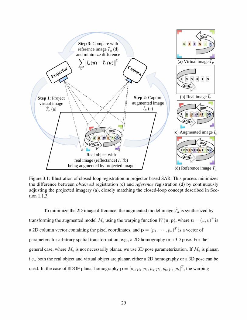
Step 3: Compare withreference image �� (d)

and minimize difference 通 ��岫�岻 − ��岫�岻 2

Real object with real image (reflectance) �� (b)

being augmented by projected image

Step 1: Project virtual image �� (a)

Step 2: Capture augmented image �� (c)

(a) Virtual image ��

(d) Reference image ��

(b) Real image ��

(c) Augmented image ��

Figure 3.1: Illustration of closed-loop registration in projector-based SAR. This process minimizes

the difference between observed registration (c) and reference registration (d) by continuously

adjusting the projected imagery (a), closely matching the closed-loop concept described in Sec-

tion 1.1.3.

To minimize the 2D image difference, the augmented model image Ta is synthesized by

transforming the augmented model Ma using the warping function W (u;p), where u = (u, v)T is

a 2D column vector containing the pixel coordinates, and p = (p1, · · · , pn)T is a vector of

parameters for arbitrary spatial transformation, e.g., a 2D homography or a 3D pose. For the

general case, where Ma is not necessarily planar, we use 3D pose parameterization. If Ma is planar,

i.e., both the real object and virtual object are planar, either a 2D homography or a 3D pose can be

used. In the case of 8DOF planar homography p = [p1, p2, p3, p4, p5, p6, p7, p8]T

, the warping

29

function becomes

W (u;p) =1

1 + p7u+ p8v

(1 + p1)u+ p3v + p5

p2u+ (1 + p4)v + p6

(3.2)

And its Jacobian can be computed as (Baker and Matthews, 2004)

∂W

∂p=

1

1 + p7u+ p8v

u 0 v 0 1 0 −u[(1+p1)u+p3v+p5]1+p7u+p8v

−v[(1+p1)u+p3v+p5]1+p7u+p8v

0 u 0 v 0 1 −u[p2u+(1+p4)v+p6]1+p7u+p8v

−v[p2u+(1+p4)v+p6]1+p7u+p8v

(3.3)

For projector-based SAR, the augmented image is a function of light and surface

reflectance. Assuming no environmental light and that the real object is planar and diffuse, then the

observed augmented image Ia can be approximated as a multiplicative modulation of the projected

light Tv, called the virtual image, the surface reflectance Ir, called the real image, and the cosine

angle between the surface normal and projector light:

Ia(u) = Tv(W (u;p)) · Ir(u) · cos θ (3.4)

where the virtual image Tv is warped onto the coordinate frame of the real image Ir. The coordinate

frames of Ia and Ir are the same. Plugging Equation (3.4) into Equation (3.1), we obtain

∑

u

‖Tv(W (u;p)) · Ir(u) · cos θ − Ta(W (u;p))‖2 (3.5)

Note that both Tv and Ta are warped using the same warping parameters since they essentially have

the same behavior. That is, we simultaneously track the real object Ir and minimize misregistration

by continuously adjusting/warping the projected virtual image. An example is shown in Figure 3.2.

Thus a nonlinear optimization problem is formulated.

30

Augmented model image ��岫�岫�; �岻岻Virtual image ��岫�岫�; �岻岻Augmented

Image ��岫�岻 R

30 degrees (misregistered)

R

V R

V

RV

15 degrees (misregistered)

0 degree (registered)

Frame N Frame N+1 Frame N+2

Figure 3.2: An example showing that the augmented model image Ta and the virtual image Tv are

warped using the same geometric transformation. Assume the real object (with the letter ‘R’) is

moved in frame N-1 and static from frame N to N+2. To track the unknown motion of the real

object, we iteratively warp both the augmented model image and the virtual image in frame N and

N+1 using the incrementally updated parameter p in each frame until the augmented image matches

the augmented model image in frame N+2. Note that the virtual image is projected onto the real

object in each frame, forming the augmented image.

To simplify the first term in Equation (3.5), we apply a logarithmic transformation to

linearize it:∑

u

‖Tv(W (u;p)) + Ir(u) + log cos θ − Ta(W (u;p))‖2 (3.6)

where Tv, Ir , and Ta are referred as the log virtual image, log real image and log augmented model

image, respectively. Likewise, the augmented image Ia also has a log form Ia:

Ia(u) = Tv(W (u;p)) + Ir(u) + log cos θ (3.7)

31

Equation (3.6) can be effectively solved using conventional gradient descent techniques. In

our implementation, we use the Gauss-Newton method to solve the problem, and apply an additive

rule to update the motion parameters (Lucas and Kanade, 1981; Baker and Matthews, 2004). The

solution of Equation (3.6) is:

∆p = −H−1∑

u

[

(▽Tv − ▽Ta)∂W

∂p

]T

E(u) (3.8)

p← p+∆p (3.9)

where ∆p is the incremental motion vector, ▽Tv and ▽Ta are gradients of Tv and Ta before

warping, E(u) denotes the error image, i.e.,

E(u) = Ia(u)− Ta(W (u;p)) (3.10)

and H is (Gauss-Newton approximation to the) Hessian matrix:

H =∑

u

[

(▽Tv − ▽Ta)∂W

∂p

]T [

(▽Tv − ▽Ta)∂W

∂p

]

(3.11)

A summary of the algorithm is shown in Algorithm 1. The ProCam system is assumed to be

geometrically calibrated. Note that in the solution Equation (3.8), it is not necessary to compute the

angle between the surface normal and the projector light for computing the log augmented image

Ia(u) as in Equation (3.7). The reason is that in SAR, the augmented images are “computed”

(combined) optically. To get the augmented image, we project the virtual image onto the scene then

capture the resulting appearance using a camera. Hence, in Algorithm 1, Ia(u) is implicitly

“computed” by capturing the scene and then performing a logarithmic transformation.

3.1.2 Empirical Validation

The following experiment was performed to validate the algorithm for SAR. A ProCam

application similar to (Audet et al., 2010) was built, where parts of the expected imagery are

32

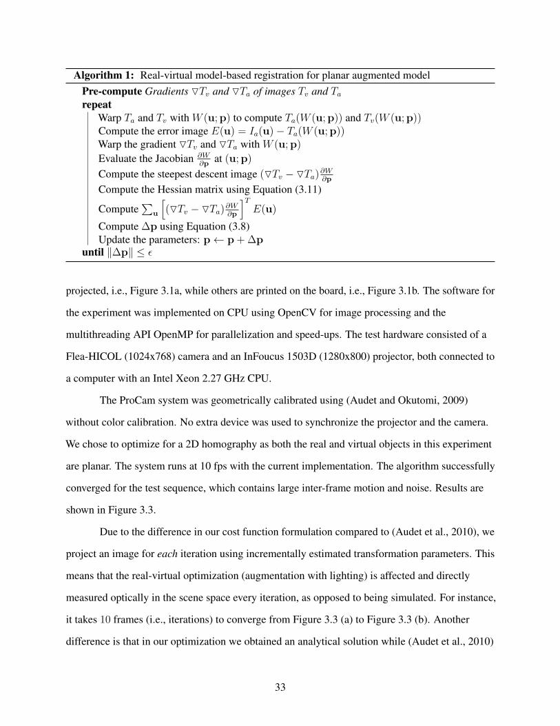
Algorithm 1: Real-virtual model-based registration for planar augmented model

Pre-compute Gradients ▽Tv and ▽Ta of images Tv and Ta

repeat

Warp Ta and Tv with W (u;p) to compute Ta(W (u;p)) and Tv(W (u;p))Compute the error image E(u) = Ia(u)− Ta(W (u;p))Warp the gradient ▽Tv and ▽Ta with W (u;p)

Evaluate the Jacobian ∂W∂p

at (u;p)

Compute the steepest descent image (▽Tv − ▽Ta)∂W∂p

Compute the Hessian matrix using Equation (3.11)

Compute∑

u

[

(▽Tv − ▽Ta)∂W∂p

]T

E(u)

Compute ∆p using Equation (3.8)

Update the parameters: p← p+∆p

until ‖∆p‖ ≤ ǫ

projected, i.e., Figure 3.1a, while others are printed on the board, i.e., Figure 3.1b. The software for

the experiment was implemented on CPU using OpenCV for image processing and the

multithreading API OpenMP for parallelization and speed-ups. The test hardware consisted of a

Flea-HICOL (1024x768) camera and an InFoucus 1503D (1280x800) projector, both connected to

a computer with an Intel Xeon 2.27 GHz CPU.

The ProCam system was geometrically calibrated using (Audet and Okutomi, 2009)

without color calibration. No extra device was used to synchronize the projector and the camera.

We chose to optimize for a 2D homography as both the real and virtual objects in this experiment

are planar. The system runs at 10 fps with the current implementation. The algorithm successfully

converged for the test sequence, which contains large inter-frame motion and noise. Results are

shown in Figure 3.3.

Due to the difference in our cost function formulation compared to (Audet et al., 2010), we

project an image for each iteration using incrementally estimated transformation parameters. This

means that the real-virtual optimization (augmentation with lighting) is affected and directly

measured optically in the scene space every iteration, as opposed to being simulated. For instance,

it takes 10 frames (i.e., iterations) to converge from Figure 3.3 (a) to Figure 3.3 (b). Another

difference is that in our optimization we obtained an analytical solution while (Audet et al., 2010)

33

(a) Frame 28: misregistered (b) Frame 38: registered

(c) Frame 118: misregistered (d) Frame 126: registered

(e) Frame 176: misregistered (f) Frame 205: registered

Figure 3.3: Qualitative evaluation of RV-MBR in SAR. Three misregistered frames due to user

motion are shown in (a), (c) and (e). Our approach observes the augmented imagery and minimizes

any visible misregistration. The corresponding registered frames are shown in (b), (d) and (f).

34

Table 3.1: Summary of mathematical notations for SAR and VST-AR.

Symbol Projector-Based Spatial AR (SAR) Video See-Through AR (VST-AR)

Ia Augmented image (i.e., camera image) N/A

Ta Augmented model image N/A

Ir Real image (surface reflectance) N/A

Tr Real model image (not used) N/A

Tv Virtual (model) image N/A

Ia Log augmented image Augmented image

Ta Log augmented model image Augmented model image

Ir Log real image Real image (i.e., camera image)

Tr Log real model image (not used) Real model image

Tv Log virtual (model) image Virtual (model) image

Ma Augmented model

Mr Real model

Mv Virtual model

evaluated the Jacobians numerically. Moreover, even without color calibration or synchronization

between the projector and the camera, the method worked well and was robust in handling the test

sequences.

3.1.3 Extension to VST-AR

To extend the approach to VST-AR, where the real and virtual do not coexist in the same

space, the augmented image Ia needs to be generated via simulation rather than being combined

optically and captured with a camera, as in SAR. To simplify the notation we use Ia, Ta, Ir and Tv

to represent augmented image, augmented model image, real image and virtual image in VST-AR,

instead of using them as log images. The reason is that in VST-AR we can simplify the real-virtual

relationship to linear math thus the logarithmic transformation is no longer needed. A simple way

to do this, similar to differential rendering (Debevec, 1998), is to consider the relationship as

addition, i.e.,

Ia = Tv + Ir (3.12)

That is, we compute the augmented image Ia as the addition of the real image (i.e., the camera

image) Ir and the virtual image Tv.

35

(a) Real model Mr (b) Virtual model Mv (c) Augmented model Ma

(d) Real/camera image Ir (e) Virtual image Tv (f) Augmented image Ia

Figure 3.4: Illustration of augmented image formulation in VST-AR. The augmented model Ma

(c) is the combination/composition (◦) of the real model Mr (a) and the virtual model Mv (b) with

correct relative 3D pose. In this example, the augmented model (c) is composited by placing the

virtual 3D model (“bunny”) onto the real textured plane (a) using a graphics engine (e.g., OpenGL).

When Ma and Mr are transformed using the warping function W (u;p) and projected onto the

virtual camera’s image plane, we obtain the augmented model image Ta and the real model image

Tr, respectively. By subtracting Tr from Ta, we obtain the virtual image Tv (e), which captures the

texture of the real model Mr (note the difference in the bunny region between (b) and (e)). Finally,

the augmented image Ia (f) is the addition of the real image (i.e., the camera image) Ir (d) and Tv

(e). It is later shown in Section 3.2.1.1 that the texture of the real model captured in the virtual

image it is useful for misregistration visualization. Note that this is a synthetic example where the

real model (a) with known ideal pose and the camera image (d) with unknown pose (to be estimated)

are synthetic. If (a) and (d) were captured/synthesized at the same camera pose, the augmented

image (f) and the augmented model view (c) would be the same, i.e., no real-virtual misregistration.

Then to compute the virtual image Tv, we can simply subtract the real model image Tr from

the augmented model image Ta, i.e.,

Tv = Ta − Tr (3.13)

An illustration of the various images and computations is shown in Figure 3.4. With this simplified

relationship between the real and virtual images, Algorithm 1 can be used almost without change

for VST-AR. We name this extended method as extended model-based registration (E-MBR).

36

(a) Real object (b) Frame 1 (c) Frame 106

Figure 3.5: Qualitative evaluation of E-MBR in VST-AR and VST-DR. For a single static camera

view with a known static background, we tracked the real planar object (a), while “camouflaging”

its “closed” window and augmenting it with an “opened” window. Results of two frames are shown

in (b) and (c).

The mathematical notations for SAR and VST-AR are summarized in Table 3.1. Note that

the real image Ir in VST-AR is the camera image, while in SAR it represents the surface reflectance

of the real object with logarithmic transformation. The reason is that the camera image in SAR

captures the appearance of the real object modulated by the projected light (i.e, virtual image Tr),

so it represents the augmented image Ia.

A qualitative evaluation was performed to show the feasibility of E-MBR in VST-AR as

well as Video See-Through Diminished Reality (VST-DR). Diminished Reality (DR) is a special

form of AR, which removes an object or collection of objects and replaces it with an appropriate

background image (Zokai et al., 2003). It can be considered a real-virtual registration process

where the objects are tracked and augmented with virtual content that hides them. DR can also be

realized using video see-through, optical see-through and projection-based displays. The result is

shown in Figure 3.5.

3.1.3.1 Numerical Comparison with Open-Loop Approach

Two quantitative experiments were conducted, the results of which show that the

closed-loop approach outperforms the conventional open-loop approach in terms of registration

accuracy. ARToolKit (Kato and Billinghurst, 1999) was chosen as the conventional open-loop

approach, as it is widely used in current AR systems. Both of the test sequences used were

synthetic so that we could also calculate the absolute ground-truth registration data easily and have

37

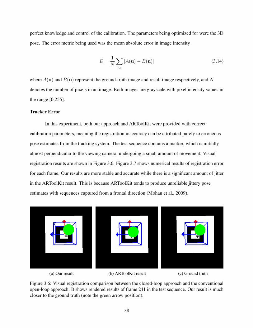
perfect knowledge and control of the calibration. The parameters being optimized for were the 3D

pose. The error metric being used was the mean absolute error in image intensity

E =1

N

∑

u

|A(u)− B(u)| (3.14)

where A(u) and B(u) represent the ground-truth image and result image respectively, and N

denotes the number of pixels in an image. Both images are grayscale with pixel intensity values in

the range [0,255].

Tracker Error

In this experiment, both our approach and ARToolKit were provided with correct

calibration parameters, meaning the registration inaccuracy can be attributed purely to erroneous

pose estimates from the tracking system. The test sequence contains a marker, which is initially

almost perpendicular to the viewing camera, undergoing a small amount of movement. Visual

registration results are shown in Figure 3.6. Figure 3.7 shows numerical results of registration error

for each frame. Our results are more stable and accurate while there is a significant amount of jitter

in the ARToolKit result. This is because ARToolKit tends to produce unreliable jittery pose

estimates with sequences captured from a frontal direction (Mohan et al., 2009).

(a) Our result (b) ARToolKit result (c) Ground truth

Figure 3.6: Visual registration comparison between the closed-loop approach and the conventional

open-loop approach. It shows rendered results of frame 241 in the test sequence. Our result is much

closer to the ground truth (note the green arrow position).

38

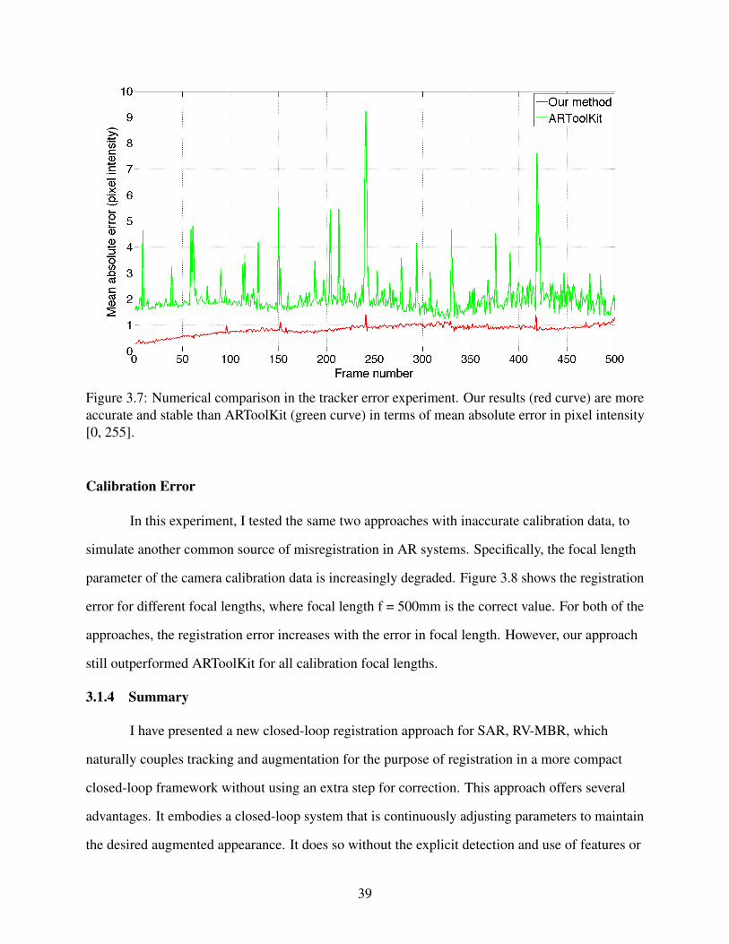
Figure 3.7: Numerical comparison in the tracker error experiment. Our results (red curve) are more

accurate and stable than ARToolKit (green curve) in terms of mean absolute error in pixel intensity

[0, 255].

Calibration Error

In this experiment, I tested the same two approaches with inaccurate calibration data, to

simulate another common source of misregistration in AR systems. Specifically, the focal length

parameter of the camera calibration data is increasingly degraded. Figure 3.8 shows the registration

error for different focal lengths, where focal length f = 500mm is the correct value. For both of the

approaches, the registration error increases with the error in focal length. However, our approach

still outperformed ARToolKit for all calibration focal lengths.

3.1.4 Summary

I have presented a new closed-loop registration approach for SAR, RV-MBR, which

naturally couples tracking and augmentation for the purpose of registration in a more compact

closed-loop framework without using an extra step for correction. This approach offers several

advantages. It embodies a closed-loop system that is continuously adjusting parameters to maintain

the desired augmented appearance. It does so without the explicit detection and use of features or

39

(a) Our result (b) ARToolKit result

Figure 3.8: Comparison of registration accuracy with different amounts of error in focal length

calibration. Our result (a) is better and contains less registration error than ARToolKit (b). The error

metric is mean absolute error in pixel intensity [0,255].

points in the camera imagery, instead optimizing the parameters directly using any misregistration

manifested in the augmented imagery. In addition to simplifying the closed-loop registration, this

approach can use information implicit in the augmented imagery, such as misregistration

manifested in the form of T-junctions or other features that do not exist in either the real or the

virtual imagery, but arise as a result of interactions between the real and virtual imagery. Our

approach can be used by itself in cases where inter-frame movement is relatively small (where the

misregistration is correctable by an iterative optimization), or in combination with a conventional

open-loop approach by using the open-loop tracking for a coarse pose estimate prior to closed-loop

optimization. Finally, the approach can be used with SAR as well as VST-AR and VST-DR such as

on hand-held or head-worn devices.

40

3.2 Closed-Loop Video See-Trough AR

In this section, I present closed-loop VST-AR, which employs a novel global-local

closed-loop registration framework to minimize misregistration in both global world space via

camera pose refinement and local screen space via pixel-wise adjustments.

Due to the fundamental difference in combining the real and virtual in SAR (light

projection) and VST-AR (digital synthesis), registration error detection in VST-AR can be achieved

with a model of the real scene, instead of an augmented model combining both the real scene model

and the virtual augmentations. Misregistration can be measured as the image difference between

the real model image—an image rendered from the real scene model using the same projection and

viewing parameters as the augmentations, and the current camera image. When any misregistration

is detected, it should be minimized in three-dimensional (3D) space. If the real model image

matches the camera image, augmentations that are registered to the real scene model will be

registered to the camera image.

The above render-compare process suggests that conventional model-based tracking (MBT)

or tracking-by-synthesis approaches (Li et al., 1993; Reitmayr and Drummond, 2006; Simon, 2011)

are already performing closed-loop registration. As shown in Figure 3.9, our proposed approach

differs from such conventional methods in two aspects: (1) we perform both global pose refinement

and local pixel-wise adjustments to deal with both rigid and non-rigid registration errors, and (2) we

enhance conventional MBT with importance weighting that weights important image regions that

have registered virtual objects, which can guide pose refinement towards better registration, even in

the presence of modeling errors. For example, when there are errors in the real scene model,

conventional methods may compute pose estimates that agree with some parts of the model, but not

other parts where augmentations are overlaid, resulting in misregistration as shown in Figure 3.11.

Our notion of “closed loop” may be considered an extension of Bajura and Neumann’s

work (Bajura and Neumann, 1995), which uses a relatively simple representation of the real

scene—one point fiducial per virtual object—and hence errors cannot be minimized in a way that

ensures complete spatial and visual coherence. By using an augmented model comprised of the real

41

Rendermodel

TrackRender

composition

Input

Image

Updated model image

Output

Image

Updated

Pose

Final

Pose

(a) Conventional closed-loop registration based on model-based tracking.

Rendermodel

TrackRender

composition

Input

Image

Updated model image & weight

Output

Image

Compute Optical Flow

Pixel-wise

corrections

Final model image

Updated

Pose

Final

Pose

(b) Our proposed closed-loop registration with global-local misregistration minimization.

Figure 3.9: Comparison between conventional closed-loop registration and our closed-loop registra-

tion.

scene model and the desired virtual augmentations, our approach can fully minimize errors in 3D.

Though real scene model alone suffices for misregistration detection, virtual augmentations can

provide important information for misregistration minimization. The important information used

here is real-virtual association—that is, one typically knows where to overlay the virtual objects

relative to the modeled real scene. In addition, with the availability of cheap 3D sensors,

reconstruction of a real scene is not difficult any more for most scenarios. The availability of an

augmented model is the starting point for the work presented here for closed-loop VST-AR.

The proposed global-local misregistration minimization process is outlined as follows. We

first employ model-based tracking (MBT) or registration-enforcing model-based tracking

(RE-MBT) to improve camera pose estimates obtained from any conventional tracking method.

This can effectively minimize rigid registration errors caused by erroneous camera pose estimates.

Even after camera pose refinement there might still exist registration errors, e.g., because of

42

uncorrected pose errors or non-rigid error sources. To deal with these residual errors we

subsequently compute the optical flow between the camera image and the real model image

rendered with the refined pose, and use the estimated flow to directly minimize misregistration in

screen space, on a per-pixel basis. The “screen space” can be equivalent to the real camera image

space, i.e., we warp the augmentations into the real camera image, obtaining registration in the

camera image. Alternatively, the “screen space” can be equivalent to the virtual camera image

space, i.e., we warp the real camera image into the virtual camera image space, resulting in

Augmented Virtuality (AV) (Milgram et al., 1995). The forward method is called forward-warping

Augmented Reality (FW-AR), while the backward method backward-warping Augmented

Virtuality (BW-AV).

3.2.1 Global World-Space Misregistration Minimization

In this section, we describe registration-enforcing model-based tracking (RE-MBT), which

can refine camera pose estimates from any existing tracking approach to achieve better registration,

even in the case of modeling errors. Our method relies on a textured 3D model of the scene to be

tracked, and the desired augmentations. We first present an overview of the conventional

model-based tracking (MBT) approach, then present how to enhance it with registration

enforcement by weighting.

3.2.1.1 3D Model-Based Tracking

Given a 3D model of the real scene, model-based tracking (MBT) aims to estimate the

6DOF camera pose p by aligning a synthesized real model image Tr with the camera image (i.e.,

real image) Ir to obtain

p = argminp

∑

x

‖ Ir(x)− Tr(W (x;p))‖2 (3.15)

where W is a warping-by-rendering function for obtaining model color and depth according to

camera pose p at an image pixel x = [x, y]T . W combines rigid motion [ R | t ]3×4 and camera

43

projection π by

W (x;p) = π(RX+ t) (3.16)

where X = [X, Y, Z]T denotes a 3D point in world coordinates, and R ∈ SO(3) and

t = [tx, ty, tz]T ∈ R

3 are the rotation matrix and translation vector. We use the exponential map of

the Lie group SE(3) to represent the rotation matrix R (Xiao et al., 2002; Ma et al., 2003):

W =

1 −wz wy tx

wz 1 −wx ty

−wy wx 1 tz

0 0 0 1

(3.17)

where [wx, wy, wz] represents the rotations relative to the three axes, and [tx, ty, tz] the 3D

translation. Hence camera pose p can be minimally represented as a 6D vector

p = [wx, wy, wz, tx, ty, tz]T

.

After transforming a point from the world coordinates to the camera coordinates, it is

projected into the image coordinate frame using a 3D-to-2D mapping π based on the camera

calibration:

x = π(X) =

fxXZ+ cx

fyYZ+ cy

(3.18)

where (fx, fy) is the focal length distance expressed in horizontal and vertical pixels, and (cx, cy) is

the principle point of the camera.

Given camera projection π and rigid motion [R | t ]3×4, the color and depth of the model in

camera coordinates can be obtained efficiently through OpenGL rendering. The cost function in

Equation (3.15) can be effectively minimized using a Gauss-Newton approach (Baker and

Matthews, 2004). The algorithm is summarized in Algorithm 2.

44

Algorithm 2: Model-based tracking

repeat

Transform Mr with W (u;p) to compute Tr(W (u;p))Compute the error image E(u) = Ir(u)− Tr(W (u;p))Compute the gradient image ▽Tr(W ) of the warped image Tr(W (u;p))

Evaluate the Jacobian ∂W∂p

at (u;p)

Compute the steepest descent image ▽Tr(W )∂W∂p

Compute the Hessian matrix H =∑

u

[

▽Tr(W )∂W∂p

]T [

▽Tr(W )∂W∂p

]

Compute∑

u

[

(▽Tv − ▽Ta)∂W∂p

]T

E(u)

Compute ∆p = −H−1∑

u

[

▽Tr(W )∂W∂p

]T

E(u)

Update the parameters: p← p+∆p

until ‖∆p‖ ≤ ǫ

Relationship with Extended Model-Based Registration (E-MBR)

Back to Section 3.1.3, if we plug both Equation (3.12) and Equation (3.13)

into Equation (3.1), we obtain the cost function of MBT, i.e., Equation (3.15). Therefore, E-MBR is

mathematically equivalent to MBT. A good use of E-MBR is that it can be used as an effective

visualization tool to show the iterative registration error reduction process with some extra

computations. Figure 3.10 shows the progression from an initial state with some noise and large

registration error to reduced error and finally almost no registration error after nine iterations for a

single frame.

3.2.1.2 Registration-Enforcing Model-Based Tracking

The conventional cost formulation in Equation (3.15) seeks the best image alignment of the

model to the input camera image, without considering the desired augmentations. This can result in

misregistration in the presence of modeling errors, as shown in Figure 3.11 (c) and (e). To make

conventional model-based tracking “aware” of the registration effects, we use a simple but effective

weighting approach:

p = argminp

∑

x

Mask(x)‖ Ir(x)− Tr(W (x;p))‖2 (3.19)

45

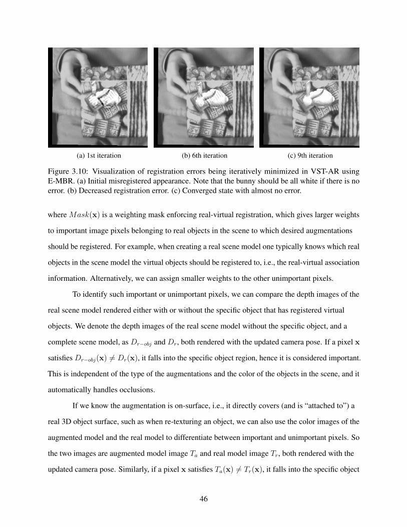
(a) 1st iteration (b) 6th iteration (c) 9th iteration

Figure 3.10: Visualization of registration errors being iteratively minimized in VST-AR using

E-MBR. (a) Initial misregistered appearance. Note that the bunny should be all white if there is no

error. (b) Decreased registration error. (c) Converged state with almost no error.

where Mask(x) is a weighting mask enforcing real-virtual registration, which gives larger weights

to important image pixels belonging to real objects in the scene to which desired augmentations

should be registered. For example, when creating a real scene model one typically knows which real

objects in the scene model the virtual objects should be registered to, i.e., the real-virtual association

information. Alternatively, we can assign smaller weights to the other unimportant pixels.

To identify such important or unimportant pixels, we can compare the depth images of the

real scene model rendered either with or without the specific object that has registered virtual

objects. We denote the depth images of the real scene model without the specific object, and a

complete scene model, as Dr−obj and Dr, both rendered with the updated camera pose. If a pixel x

satisfies Dr−obj(x) 6= Dr(x), it falls into the specific object region, hence it is considered important.

This is independent of the type of the augmentations and the color of the objects in the scene, and it

automatically handles occlusions.

If we know the augmentation is on-surface, i.e., it directly covers (and is “attached to”) a

real 3D object surface, such as when re-texturing an object, we can also use the color images of the

augmented model and the real model to differentiate between important and unimportant pixels. So

the two images are augmented model image Ta and real model image Tr, both rendered with the

updated camera pose. Similarly, if a pixel x satisfies Ta(x) 6= Tr(x), it falls into the specific object

46

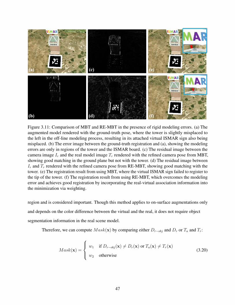
Figure 3.11: Comparison of MBT and RE-MBT in the presence of rigid modeling errors. (a) The

augmented model rendered with the ground-truth pose, where the tower is slightly misplaced to

the left in the off-line modeling process, resulting in its attached virtual ISMAR sign also being

misplaced. (b) The error image between the ground-truth registration and (a), showing the modeling

errors are only in regions of the tower and the ISMAR board. (c) The residual image between the

camera image Ir and the real model image Tr rendered with the refined camera pose from MBT,

showing good matching in the ground plane but not with the tower. (d) The residual image between

Ir and Tr rendered with the refined camera pose from RE-MBT, showing good matching with the

tower. (e) The registration result from using MBT, where the virtual ISMAR sign failed to register to

the tip of the tower. (f) The registration result from using RE-MBT, which overcomes the modeling

error and achieves good registration by incorporating the real-virtual association information into

the minimization via weighting.

region and is considered important. Though this method applies to on-surface augmentations only

and depends on the color difference between the virtual and the real, it does not require object

segmentation information in the real scene model.

Therefore, we can compute Mask(x) by comparing either Dr−obj and Dr or Ta and Tr:

Mask(x) =

w1 if Dr−obj(x) 6= Dr(x) or Ta(x) 6= Tr(x)

w2 otherwise

(3.20)

47

As introduced above, we can either fix w2 = 1 and increase w1 to be larger than w2, or fix

w1 = 1 and decrease w2 to zero. The former requires some heuristics to determine a value for w1,

while the latter does not.

By re-evaluating the weighting mask during each iteration, Equation (3.19) becomes an

iteratively reweighted least squares (IRLS) problem (Simon Baker and Matthews, 2003). Though it

might seem a simple enhancement over conventional MBT, our use of weighting is the first

approach that incorporates the real-virtual association information into the error minimization

process. As such it is more effective in improving camera pose estimates towards better registration,

compared to conventional MBT, especially when there are errors in the real model. In the example

shown in Figure 3.11 (d) and (f), RE-MBT overcomes the modeling error and improves registration,

while conventional MBT fails shown in Figure 3.11 (c) and (e).

The cost function in Equation (3.19) only models brightness constancy, i.e., it assumes that

the intensity of the model image Tr and the camera image Ir match. However, this assumption is

easily violated in practice due to factors such as camera auto-exposure mechanisms and lighting

changes. Therefore, we generalize the method to include a linear photometric compensation term:

p = argminp,g,b

∑

x

Mask(x)‖ gIr(x) + b− Tr(W (x;p))‖2 (3.21)

where g and b are 3D vectors modeling the camera gain and bias for each color channel, to account

for global color differences (Bartoli, 2008). These parameters can be applied to the rendered

augmentations to make them appear less artificial and more visually plausible, as introduced in

Section 3.2.4.

3.2.2 Local Screen-Space Misregistration Minimization

After world-space registration error minimization by camera pose refinement, there might

still exist registration errors, for example, because of uncorrected pose errors or non-rigid error

sources. To deal with these residual errors, we subsequently compute the optical flow (OF) between

48

the camera image Ir and the model image Tr rendered with the refined pose, and use the estimated

flow to directly minimize misregistration in screen space, on a per-pixel basis.

We propose two distinct ways of using the estimated flow u to improve the final registration

results: Forward-Warping Augmented Reality (FW-AR) and Backward-Warping Augmented

Virtuality (BW-AV). The relative advantage and disadvantage of the methods are explained and

demonstrated in Figure 3.12.

The optical flow (OF) is a 2D displacement field defined as u = [u, v]T , representing the

apparent motion of the brightness patterns in the image (Horn and Schunk, 1981). In our

screen-space registration error minimization, for forward warping, the flow u is computed from the

current model image Tr to the current camera image Ir, i.e., Tr(x) = Ir(x+ u); for backward

warping, it is computed from the current camera image Ir to the current model image Tr , i.e.,

Ir(x) = Tr(x+ u). The color of the camera image Ir is adjusted with the estimated gain and bias

prior to the OF computation.

3.2.2.1 Forward-Warping Augmented Reality

FW-AR refers to registration error minimization in the real camera space by using the

estimated flow to warp any augmentations rendered with the refined camera pose into the camera

image. This has the advantage of maintaining the “reality” observed by the camera, i.e., keeping the

camera image Ir the same as traditional AR registration, and it can enhance the realism of the

augmentations by acquiring real object surface properties from the flow that are not modeled in the

augmentations. To name a few examples, surface properties can be deformation, crumples, or even

tearing. As shown in Figure 3.14, the forward warping results in MBT & FW-AR (c) and RE-MBT

& FW-AR (g) contain the desired un-modeled “bent” effects in the virtual “ISMAR board”, which

matches the deformation of the underlying real ground plane.

Given the 2D nature of OF, the estimated flow does not provide meaningful displacement

for virtual object pixels closer to the camera than the real object surface. Therefore FW-AR is best

for on-real-object-surface augmentations, e.g., for object re-texturing. The greater the depth

49

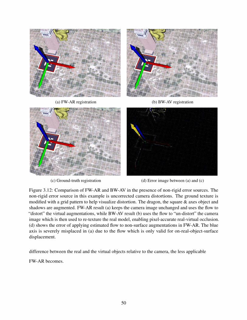
(a) FW-AR registration (b) BW-AV registration

(c) Ground-truth registration (d) Error image between (a) and (c)

Figure 3.12: Comparison of FW-AR and BW-AV in the presence of non-rigid error sources. The

non-rigid error source in this example is uncorrected camera distortions. The ground texture is

modified with a grid pattern to help visualize distortion. The dragon, the square & axes object and

shadows are augmented. FW-AR result (a) keeps the camera image unchanged and uses the flow to

“distort” the virtual augmentations, while BW-AV result (b) uses the flow to “un-distort” the camera

image which is then used to re-texture the real model, enabling pixel-accurate real-virtual occlusion.

(d) shows the error of applying estimated flow to non-surface augmentations in FW-AR. The blue

axis is severely misplaced in (a) due to the flow which is only valid for on-real-object-surface

displacement.

difference between the real and the virtual objects relative to the camera, the less applicable

FW-AR becomes.

50

3.2.2.2 Backward-Warping Augmented Virtuality

BW-AV refers to registration error minimization in virtual camera screen space by using the

estimated flow to warp the camera image Ir into the virtual camera image, which in effect

re-textures the real model rendered with the refined camera pose. In other words, the camera image

is warped and displayed as background. The biggest advantage of BW-AV is that it preserves the

full use of the dense geometry buffer (G-buffer) provided by the augmented model, enabling the

best 3D registration at the level of G-buffer accuracy.

The disadvantage of BW-AV is that “reality” observed by the camera is altered, yielding an

Augmented Virtuality (AV) image. However, the AV imagery is rendered with the refined camera

pose, hence it can appear very close to perfectly registered AR imagery.

3.2.3 Guidelines for Global-Local Misregistration Minimization

We have introduced our global-local registration error minimization approach, including

both world-space (MBT and RE-MBT) and screen-space (FW-AR and BW-AV) error minimization.

Each of the four methods has its advantages and disadvantages as described in Section 3.2.1 and

Section 3.2.2.

3.2.3.1 General Guidelines

There are four possible combinations of world-space and screen-space methods: MBT &

FW-AR, MBT & BW-AV, RE-MBT & FW-AR, and RE-MBT & BW-AV. While we present general

guidelines for choosing the right combinations in Table 3.2, those guidelines should be considered

on a case-by-case basis.

MBT aims to minimize the image difference between the model image and the camera

image in an unbiased fashion. This is desirable for BW-AV, as we would like the AV imagery to be

as close to the AR imagery as possible. In general, MBT is better for BW-AV in preserving the

“reality” than RE-MBT. However there can be exceptions. For example, as shown in Figure 3.14 (h)

and (l), the result of RE-MBT & BW-AV is closer to the AR result, because the weighting mask

enforces the registration in the majority of the real object region, i.e., the right side in the example.

51

Table 3.2: Analysis of all four combinations of world-space (MBT or RE-MBT) and screen-space

(FW-AR or BW-AV) misregistration minimization.

Property MBT RE-MBT

Property N/ASeeks best unbiased

alignment

Incorporates real-virtual

association thus “awares”

of registration

FW-AR

Preserves “reality” and

transfers desired

unmodeled surface details

to on-surface

augmentations

On-surface augmentations

of slightly deformed

objects

On-surface augmentations

of slightly deformed

objects

BW-AV

Alters “reality” but

preserves the full use of

the dense geometry buffer

provided by the

augmented model

Supports best

pixel-accurate depth

registration between the

real and the virtual

Not recommended since

model and camera image

may look too different in

case of large modeling

errors

RE-MBT can be useful when there are errors beyond those caused by camera pose, and it

can use the real-virtual association information to refine the camera pose to achieve improved

registration overall. At this time we can only improve registration with respect to a single real

object in the scene, or multiple objects that are modeled with the same confidence, since we assume

only one camera pose is computed. If there are multiple objects in the scene to be augmented and

their 3D models are available, RE-MBT can be readily applied to refine registration for each object.

In this case, it is better to use multiple object tracking methods to compute pose estimates for each

object, e.g., (Park et al., 2011; Kim et al., 2012).

FW-AR is generally preferred as it minimizes the misregistration in the real camera space.

However, due to the 2D nature of the estimated flow, it can only be used to warp augmentation

pixels that have similar depth as the underlying real object pixels where the flow is computed, with

respect to the viewing camera. This can be a significant limitation for use cases beyond

surface-based augmentations. However, if the residual flow is relatively small in a non-surface 3D

52

(a) Input camera image (b) Initial model image

Figure 3.13: Input images for the specific example.

augmentations region, such as in Figure 3.14 (g) and (j), it should not significantly alter the integrity

of the 3D appearance of the virtual object and can still be applied.

BW-AV is generally the best way to achieve pixel-accurate registration as it preserves the

full use the geometry buffer. When combining with MBT, it can typically achieve both accurate

registration and similar results to perfect AR registration.

3.2.3.2 An Example Use

Here we present a specific example to illustrate the above guidelines. The input camera

image and the initial model image rendered with the pose prior for this example are shown

in Figure 3.13. The camera image is generated using the model, which is deliberately “bent” along

its center vertical axis (the dashed red line) to simulate some modeling errors, and it is labeled

“Left” and “Right” for ease of discussion. For our closed-loop registration results, shown in

Figure 3.14, the original “unbent” model is used.

In Figure 3.14, the first column demonstrates the use of MBT, and the second column,

RE-MBT. MBT fails to find good alignment for either the left or right side, as can be seen in the

residual image (a). For RE-MBT, the weighting mask is set to the right side, as it contains the 3D

virtual dragon that requires a reliable pose estimate; hence, an improved pose is computed to

minimize the image difference in the right side, as shown in (e), but with increased error in the left

side, compared to (a). The estimated flow in (b) after MBT contains large flows in both the left and

53

right sides, which is consistent with the residual error in (a). For RE-MBT, the estimated flow in (f)

also aligns well with the residual image (e), which has large flows in the left side and there is

almost no flow in the right side.

The forward warping results in MBT & FW-AR (c) and RE-MBT & FW-AR (g) contain the

desired un-modeled “bent” effects in the “ISMAR board”, which matches the deformation of the

underlying ground plane. To better illustrate how the flow is used to warp the augmentations in

FW-AR, we use blended images of the augmentations before and after the flow, as shown in (i) and

(j). In (j), the right side is not warped, since in (f) the right side has almost zero flow; but its left side

is strongly warped, since after RE-MBT, the right side matches, but left side becomes less matched.

While in (i), the left side and the right side are both warped, resulting in an undesirable shape

change in the dragon (it is blurred in the blended image; see the zoomed-in portions of the images).

As a result, (h) using RE-MBT & BW-AV better approximates the “reality” than (d) using

MBT & BW-AV, as in this case, RE-MBT refines the camera pose for the majority of the “reality”

in the input camera image. Again, we use blended images to show the differences clearly. (k) shows

the blending of the input camera image in Figure 3.13 (a) and the MBT & BW-AV result (d), which

exhibits obvious blur in real object pixels in both left and right sides, indicating its registration

result is relatively far from AR registration. In contrast, (l) shows the blending of the same input

camera image and the RE-MBT & BW-AV result, and it is sharp in the right side, indicating the

registration result in the right side (the majority of the “reality”) is very close to the accurate AR

registration in the real camera space.

3.2.3.3 Discussion

Though FW-AR and BW-AV have their limitations, they can offer a number of practical

solutions in complex real scenarios. The possibilities include, but not limited to:

1. FW-AR and BW-AV can be dynamically interchanged based on camera pose. For

example, in the case of handheld AR, the user may move the camera freely to view

different parts of the scene that may have different augmentations (on-surface or

54

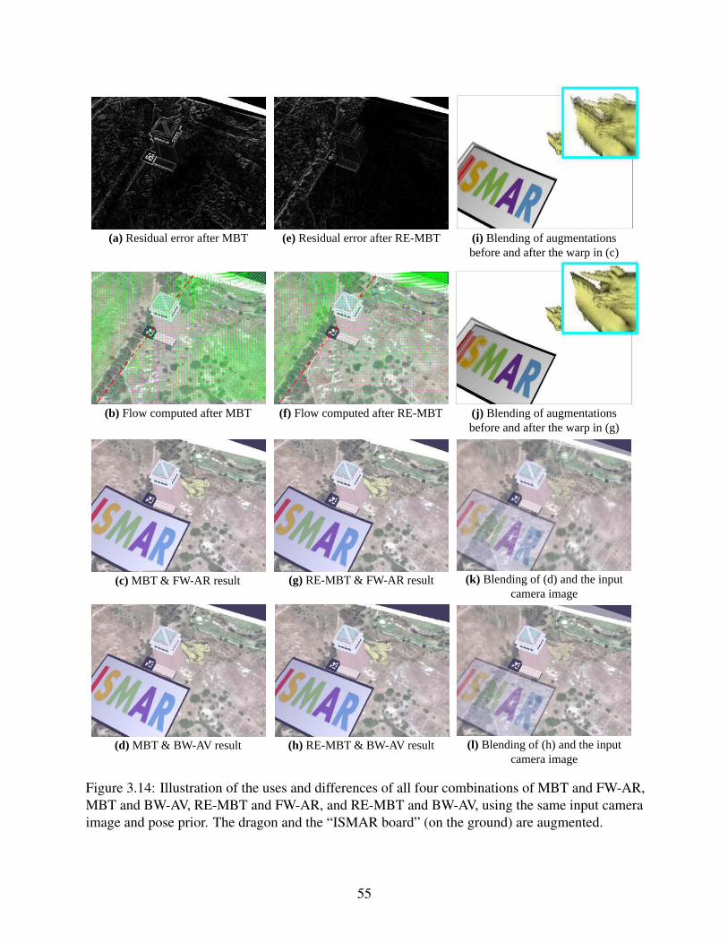
(a) Residual error after MBT

(b) Flow computed after MBT

(c) MBT & FW-AR result

(d) MBT & BW-AV result

(e) Residual error after RE-MBT

(f) Flow computed after RE-MBT

(g) RE-MBT & FW-AR result

(h) RE-MBT & BW-AV result

(i) Blending of augmentations before and after the warp in (c)

(j) Blending of augmentations before and after the warp in (g)

(k) Blending of (d) and the input camera image

(l) Blending of (h) and the input camera image

Figure 3.14: Illustration of the uses and differences of all four combinations of MBT and FW-AR,

MBT and BW-AV, RE-MBT and FW-AR, and RE-MBT and BW-AV, using the same input camera

image and pose prior. The dragon and the “ISMAR board” (on the ground) are augmented.

55

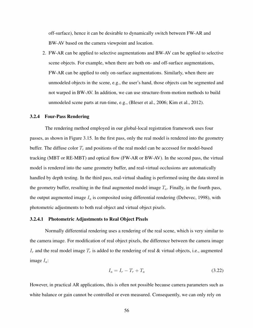
off-surface), hence it can be desirable to dynamically switch between FW-AR and

BW-AV based on the camera viewpoint and location.

2. FW-AR can be applied to selective augmentations and BW-AV can be applied to selective

scene objects. For example, when there are both on- and off-surface augmentations,

FW-AR can be applied to only on-surface augmentations. Similarly, when there are

unmodeled objects in the scene, e.g., the user’s hand, those objects can be segmented and

not warped in BW-AV. In addition, we can use structure-from-motion methods to build

unmodeled scene parts at run-time, e.g., (Bleser et al., 2006; Kim et al., 2012).

3.2.4 Four-Pass Rendering

The rendering method employed in our global-local registration framework uses four

passes, as shown in Figure 3.15. In the first pass, only the real model is rendered into the geometry

buffer. The diffuse color Tr and positions of the real model can be accessed for model-based

tracking (MBT or RE-MBT) and optical flow (FW-AR or BW-AV). In the second pass, the virtual

model is rendered into the same geometry buffer, and real-virtual occlusions are automatically

handled by depth testing. In the third pass, real-virtual shading is performed using the data stored in

the geometry buffer, resulting in the final augmented model image Ta. Finally, in the fourth pass,

the output augmented image Ia is composited using differential rendering (Debevec, 1998), with

photometric adjustments to both real object and virtual object pixels.

3.2.4.1 Photometric Adjustments to Real Object Pixels

Normally differential rendering uses a rendering of the real scene, which is very similar to

the camera image. For modification of real object pixels, the difference between the camera image

Ir and the real model image Tr is added to the rendering of real & virtual objects, i.e., augmented

image Ia:

Ia = Ir − Tr + Ta (3.22)

However, in practical AR applications, this is often not possible because camera parameters such as

white balance or gain cannot be controlled or even measured. Consequently, we can only rely on

56

(a) Real model (b) Augmented model

(c) Augmented model with shading (d) Output augmented image composition

Figure 3.15: Illustration of four-pass rendering: (a) real model rendered with the current pose

estimate, (b) virtual model rendered into the same geometry buffer with the same pose, resulting in

unshaded augmented model, (c) augmented model being shaded, and (d) output augmented image

composited via differential rendering with photometric adjustments to both real object and virtual

object pixels. The dragon, the square & axes object and shadows are augmented.

relative rather than absolute values. Via the OF we can relate camera pixels to rendered pixels of

the real model. This allows us to compute a ratio rather than a difference describing the relationship

of the camera to the rendering:

Ia = Ir/Tr w × Ta w (3.23)

for forward warping, and

Ia = Ir w/Tr × Ta (3.24)

for backward warping. Tr w and Ta w are warped from Tr and Ta, respectively, which are rendered

with the refined camera pose, and Ir w is warped from the camera image Ir.

57

Employing a ratio works for single channel intensities, but not for RGB values. However

we can transform RGB values to a L*a*b* color space, where colors are also expressed in relative

terms, and the computation above yields meaningful results.

3.2.4.2 Photometric Adjustments to Virtual Object Pixels

For virtual objects pixels, we cannot establish a relationship with camera image pixels to

compute per-pixel color adjustments. We therefore employ a simple linear adjustment using

estimated average gain and bias values for all real object pixels to camera pixel correspondences in

the scene. However, color space bias could be modeled as a tone mapping based on dynamic

camera image histograms, such as with the approach of Knecht et al. (Knecht et al., 2011). We

leave this for future work.

3.2.5 Experimental Results

We conducted experiments to evaluate our proposed global-local closed-loop registration

approach with both synthetic and real sequences.

3.2.5.1 Implementation

Our model-based tracking methods (both MBT and RE-MBT) employ the Gauss-Newton

approach (Baker and Matthews, 2004) implemented on the GPU using OpenCV with CUDA

support and OpenGL with GLSL. We directly use the existing implementation of the anisotropic

Huber-L1 optical flow (Werlberger et al., 2009) provided by the FlowLib (Werlberger and Pock,

2012). It preserves discontinuities and smoothness while still being robust to illumination changes

and noise, and is thus suitable for our basic needs for screen-space pixel-wise misregistration

minimization. Our system is currently running at 5 fps without any special optimization.

3.2.5.2 Synthetic Sequences

To evaluate and demonstrate our approach we created several synthetic sequences with

different simulated sources of error, and known ground-truth registration. These synthetic

sequences were created using the precisely tracked hand-held camera motion from the

“City-of-Sights” dataset (Gruber et al., 2010) to make them realistic and difficult. Our approach

58

passed all of the test cases, and achieved pixel-wise accurate registration. Some results are shown in

Figure 3.16.

3.2.5.3 Real Sequences

We tested several real planar sequences provided by the “City-of-Sights” dataset, which

contains rapid hand-held motion. The ground-truth pose provided in these sequences was measured

using the mechanical FARO CMM tracker that was carefully calibrated, but still results in

significant registration error when processed in a conventional open-loop AR fashion. Our

closed-loop approach uses the given pose measurements at each frame and achieves pixel accurate

registration, appearing more visually accurate as shown in Figure 3.17. Note that in the third

column in Figure 3.17, photometric adjustments to the rendering of real object pixels

(virtual-to-real shadows) and virtual object pixels (with estimated gain and bias) are turned on,

hence the result images look more visually blended into the camera image.

3.2.6 Limitations

While our closed-loop approach is widely applicable in general, and should improve the

final registration in most cases, there are some limitations. First, our world-space registration error

minimization methods will have difficulty with “large” pose errors, and our screen-space methods

will have difficulty with “large” displacements. It is difficult to quantify “large” in these cases, as

there are many factors, but it can happen (for example) that the registration error minimization

process will converge to the wrong solution. In practice, we find that this is dependent on the

quality of the pose estimation. Similarly, both world- and screen-space methods can have difficulty

with strong appearance differences between the real model image and the camera image, e.g.,

strong shadows, dramatic lighting changes, motion blur, or big occlusions. These issues are not

unique to our closed-loop approach—they are common to traditional vision-based tracking and

optical flow approaches. We have not evaluated our closed-loop approach extensively with real test

sequences, in part, because our adopted optical flow algorithm cannot handle large non-linear

photometric differences between the model and the camera image, and cannot handle strong

shadows. In addition, the estimated flow is currently used directly for screen-space registration

59

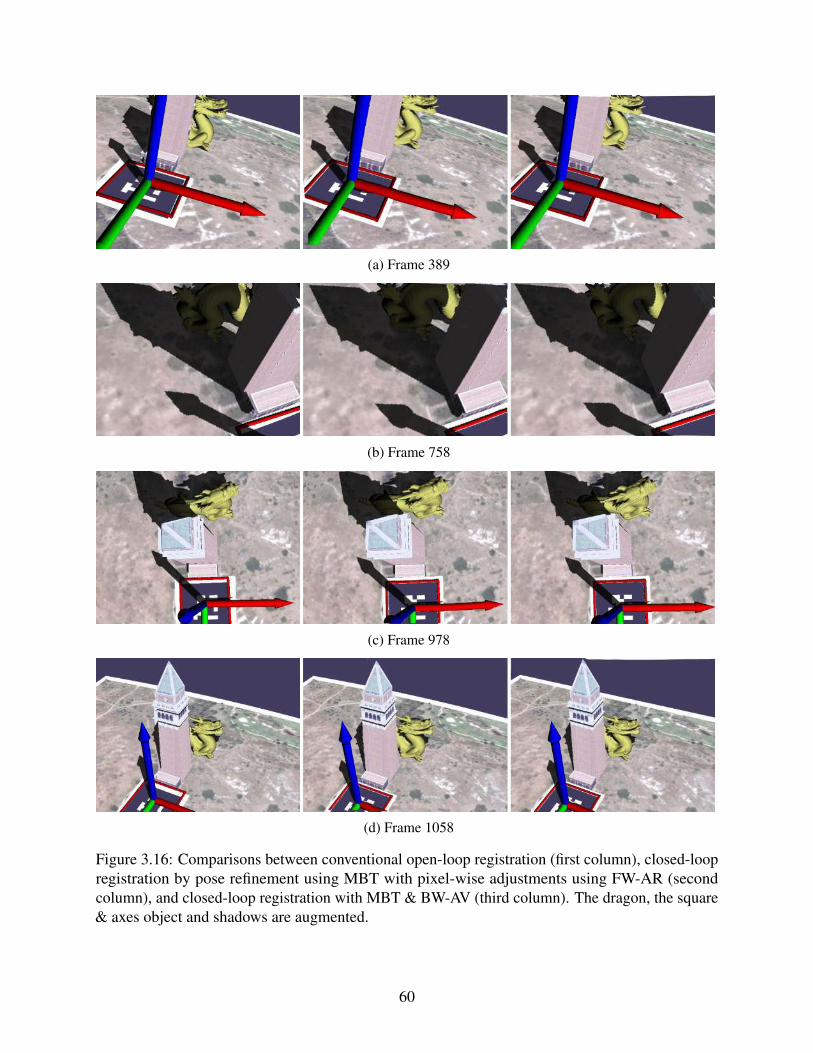
(a) Frame 389

(b) Frame 758

(c) Frame 978

(d) Frame 1058

Figure 3.16: Comparisons between conventional open-loop registration (first column), closed-loop

registration by pose refinement using MBT with pixel-wise adjustments using FW-AR (second

column), and closed-loop registration with MBT & BW-AV (third column). The dragon, the square

& axes object and shadows are augmented.

60

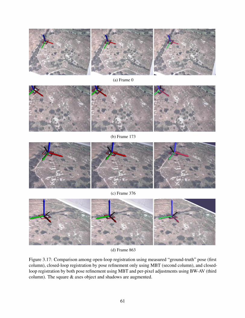
(a) Frame 0

(b) Frame 173

(c) Frame 376

(d) Frame 863

Figure 3.17: Comparison among open-loop registration using measured “ground-truth” pose (first

column), closed-loop registration by pose refinement only using MBT (second column), and closed-

loop registration by both pose refinement using MBT and per-pixel adjustments using BW-AV (third

column). The square & axes object and shadows are augmented.

61

error minimization. It could be improved with forward and backward cross-matching to prune

erroneous flow. Furthermore, the virtual object shape information provided by the G-buffer can be

used to enhance the flow to make it respect the virtual object boundaries in FW-AR.

3.2.7 Conclusion

Our closed-loop approach has its roots in conventional control theory, where one attempts

to use available measurements to estimate and control the “hidden” internal state of a complex

system. A typical approach is to iteratively estimate the system state using analytical process

models, predict the measurements using the state estimates, compute an “error” (difference) signal

between the predicted and actual measurements, and then feed some version of that error signal

back to the state estimator to minimize the (apparent) error. When one has prior knowledge about

the likely structure of the error signal, one should tailor the feedback to maximize the effectiveness

of that prior knowledge.

In our AR application of this closed-loop paradigm, the real-virtual registration error signal

is derived from rendered images of the real object models and real images from the camera, and we

know certain properties of the structure of that signal. For example, we know pose-related errors

will be related to the geometry of the scene. In addition, errors associated with certain static

image-related parameters, e.g., radial distortion, will cause consistent misregistration, if not

corrected.

Our closed-loop approach is designed to leverage this prior knowledge. We employ

model-based tracking (MBT or RE-MBT) to minimize misregistration associated with erroneous

camera pose, and optical flow techniques to measure and minimize for pixel-wise artifacts arising

from both known error sources, e.g., uncorrected pose errors, and unknown error sources such as

lens distortion and object deformation. Though our approach does have some limitations, and the

absolute accuracy of the refined pose and pixel-wise adjustments are not guaranteed, we believe

that the relative real-virtual registration accuracy and image consistency afforded by our automatic

refinement can offer an effective means for perceived accuracy and stability.

62

3.2.8 Future Work

Looking ahead, we have several enhancements in mind. For example, currently the

appearance of virtual object is enhanced using linear photometric compensation (gain and bias).

With dense per-pixel correspondence between the model and the camera image provided by the OF,

tone mapping (Knecht et al., 2011) could be employed to better compensate for differences in the

photometric spaces of the camera and the real model, making the rendered colors more closely

match those of the real camera.

The efficiency of both world- and screen-space registration error minimization methods

could be improved, in order to make the system real-time. Currently, the real model is re-rendered

with updated pose in every iteration in both MBT and RE-MBT. The rendering cost could be

reduced by rendering only once at the first iteration of each pyramid level and then using

post-rendering 3D warp (Mark et al., 1997) for subsequent iterations, as the pose change is small

across iterations in the same pyramid level. We could limit dense optical flow computation in

FW-AR only in the image regions of virtual objects rather than the entire image.

Currently our OF is used after MBT or RE-MBT, assuming they have solved any/all rigid

errors in the camera pose. That assumption might not be valid. We believe we could incorporate OF

into the closed-loop iterative refinement as well, aiming to jointly minimize the optical flow

Pixel-wise correction

Pose correction

Modelcorrection

Calibration correction

Figure 3.18: Full misregistration minimization loop.

63

between the camera and model images, while simultaneously minimizing camera pose errors.

Furthermore, based on the history of pose errors and flow fields, we could detect structured

geometric error sources, such as errors in calibration and modeling. In this way, we could fully

“close the loop”, as shown in Figure 3.18. Errors in calibration and modeling are relatively difficult

to detect in a single frame so the outer loop does not necessarily need to run in every frame. Once

these structured errors are minimized, they will typically not occur again.

64

CHAPTER 4: LOW-LATENCY TEMPORAL REGISTRATION

Among all error sources, system latency is the largest single source of registration error in

existing AR systems, outweighing all others combined (Holloway, 1997a). In this chapter, I present

low-latency temporal registration, which employs fine-grained render-display processing to

minimize both apparent latency in rendering and absolute latency in display. The apparent latency

in rendering could be minimized by a cascade of successively simpler and faster renders, each of

which responds to tracking data, in the spirit of just-in-time rendering (Section 2.3.2.2). The

absolute latency in display is minimized by a new image generation approach which operates at the

maximum internal switching rate of the display. This new image generation approach is

experimentally demonstrated with a bench-top Optical See-Through AR (OST-AR)

proof-of-concept prototype that uses a Digital Light Processing (DLP™) projector whose Digital

Micromirror Device (DMD) imaging chip is directly controlled by a computer, similar to the way

random access memory is controlled.

This chapter substantially replicates the peer-reviewed paper “Minimizing Latency for

Augmented Reality Displays: Frames Considered Harmful” published at IEEE International

Symposium on Mixed and Augmented Reality (ISMAR) in 2014 (Paper 3, co-authored with

Turner Whitted, Anselmo Lastra, Peter Lincoln, Andrei State, Andrew Maimone, and Henry Fuchs).

4.1 Latency in Optical See-Through AR

In the past several decades, AR has been shown to be useful in a variety of areas, such as

medicine, manufacturing, maintenance, navigation and telepresence. Many of these may further

benefit from head-worn, eyeglass-style displays, which are currently evolving rapidly (Microsoft,

2015; Epson, 2014; Vuzix, 2013). These displays optically combine the computer-generated image

with the user’s direct view of the surroundings (“optical see-through”), in contrast to smartphone-

65

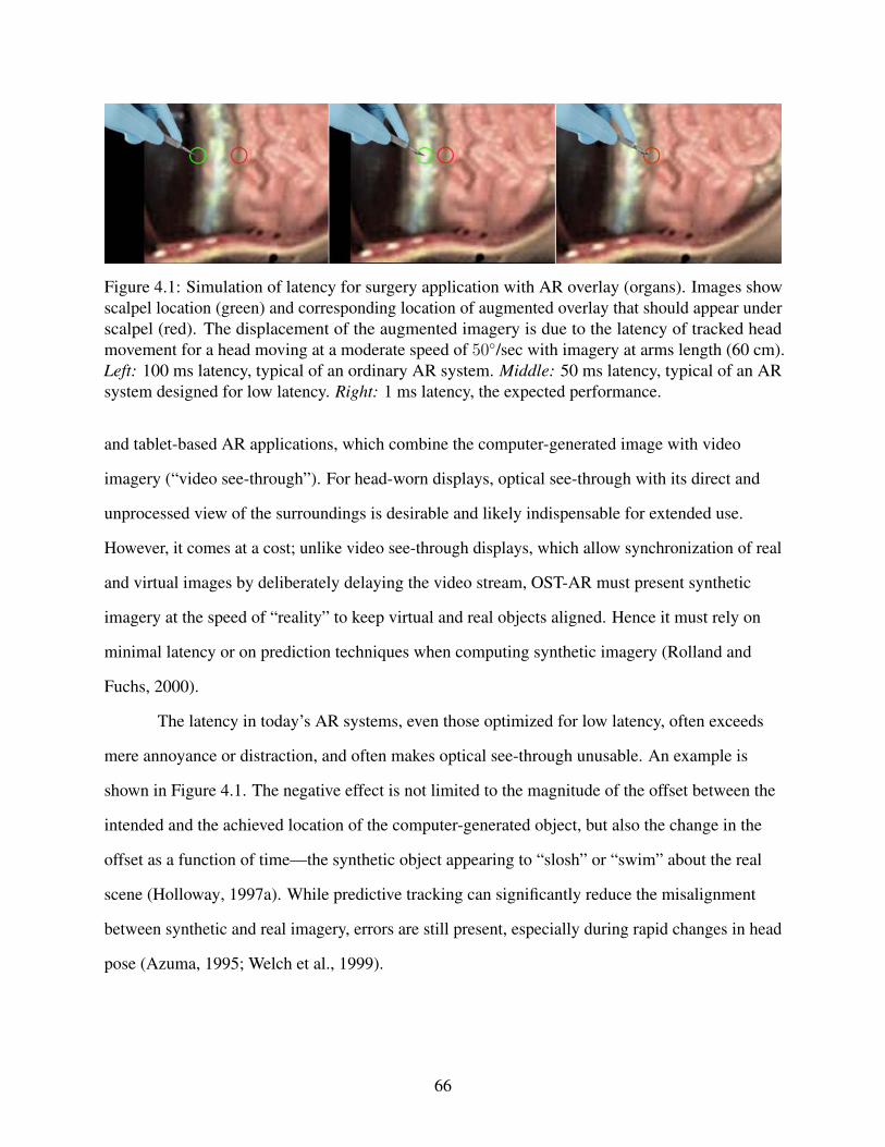
Figure 4.1: Simulation of latency for surgery application with AR overlay (organs). Images show

scalpel location (green) and corresponding location of augmented overlay that should appear under

scalpel (red). The displacement of the augmented imagery is due to the latency of tracked head

movement for a head moving at a moderate speed of 50◦/sec with imagery at arms length (60 cm).

Left: 100 ms latency, typical of an ordinary AR system. Middle: 50 ms latency, typical of an AR

system designed for low latency. Right: 1 ms latency, the expected performance.

and tablet-based AR applications, which combine the computer-generated image with video

imagery (“video see-through”). For head-worn displays, optical see-through with its direct and

unprocessed view of the surroundings is desirable and likely indispensable for extended use.

However, it comes at a cost; unlike video see-through displays, which allow synchronization of real

and virtual images by deliberately delaying the video stream, OST-AR must present synthetic

imagery at the speed of “reality” to keep virtual and real objects aligned. Hence it must rely on

minimal latency or on prediction techniques when computing synthetic imagery (Rolland and

Fuchs, 2000).

The latency in today’s AR systems, even those optimized for low latency, often exceeds

mere annoyance or distraction, and often makes optical see-through unusable. An example is

shown in Figure 4.1. The negative effect is not limited to the magnitude of the offset between the

intended and the achieved location of the computer-generated object, but also the change in the

offset as a function of time—the synthetic object appearing to “slosh” or “swim” about the real

scene (Holloway, 1997a). While predictive tracking can significantly reduce the misalignment

between synthetic and real imagery, errors are still present, especially during rapid changes in head

pose (Azuma, 1995; Welch et al., 1999).

66

Unfortunately, latency accumulates throughout all the components of an AR system

(tracking, application, rendering, scanout, display). This chapter concentrates on the latency in the

image scanout and display itself.

Today’s most common display technologies (LCD, OLED, DMD) form images through

various methods of controlling light: spatially, temporally, and in terms of wavelength (or even

polarization). Historically, and until today, these capabilities have been internally “managed” by

device designers, while end users have been limited to common display interfaces (VGA, DVI,

HDMI). While these interfaces allow plug-and-play flexibility, they impose certain restrictions that

are difficult to work around. Specifically, this abstract layer is derived from the raster scan method

(developed in the late 1930s for Cathode Ray Tube (CRT) television sets), which scanning pixels

out from the graphics card to the display left-to-right in a series of horizontal scanlines from top to

bottom (Whitton, 1984), so it introduces almost an entire video frame of latency in the display

device itself. In addition, with DMDs, color imagery is almost always delivered via

frame-sequential display—e.g., all pixels of the red channel displayed simultaneously, then all

pixels of the blue channel, then all pixels of the green channel. Therefore, a display device has to

receive an entire image before it can start to display even the first pixel of that image.

Even on simpler devices, such as a CRTs, the display of the bottom of the image occurs

much later than the display of the top of the image. Raster scan is inherently unsuited for

low-latency applications, unless scanout is performed at very high rates, which tends to cause

memory access and high-power utilization issues.

Therefore, we advocate “de-abstracting” this display interface layer and exposing the

technology underneath to the image-generation process. This will permit the image generation

processors to “get closer” to the control of the photons in the display, achieving dramatically lower

overall latencies.

4.2 General Approach

We minimize latency by updating selected parts of the displayed image—those that require

the most change—instead of the complete image. Updating arbitrary individual pixels is generally

67

Tracker20 kHz

Renderer20 Hz

Post-Rendering 3D Warp200 Hz

2D Warp2 kHz

Color + Depth

(> Disp. Res.)

Color

(> Disp. Res.)

3D rotation + 3D translation

3D rotation + 3D translation

2D rotation + 2D translation

2D Offset20 kHz

2D translation

DifferenceEstimation

Desired Image(= Disp. Res.)

Color

(> Disp. Res.)

User PerceptionEstimation

User Perceived Image(= Disp. Res.)

DisplayUpdate

Display Image (= Disp. Res.)

Low-Latency Display Image Generation

Figure 4.2: End-to-end low-latency AR pipeline. While the whole approach comprises many stages,

each operating faster than the prior stage, our current prototype implements only the low-latency

display image generation stages (in the dashed rectangle). “Disp. Res.” is short for “Display

Resolution”. The thickness of arrow lines between stages indicates the amount of data being

transfered. Note that all the frequencies are estimated.

not feasible; ideally, we would update small groups of pixels in parallel at a bandwidth as high or

higher than current full-frame bandwidth. This leads to higher update rates, albeit of smaller

display regions. While no currently available display accommodates this update mode, we propose

a broad framework for the ideal device and then specialize the algorithm for an existing one.

The goal of this algorithm is—at every update of the display—to bring the image that is

perceived by the viewer closer to an estimate of the latest true image, as determined by the tracker.

We call this estimate of the true image the Desired Image. Producing the Desired Image by

conventional rendering would be challenging at the rates at which we want to update the display,

which is on the order of tens of thousands of updates per second. We propose rendering from

polygons (or other primitives) at as high an update rate as a GPU can produce, and then computing

a 3D warp from two nearby rendered images (Mark et al., 1997) to approximate the desired image.

If a 3D warp at the desired update rate is not possible, then adding another, computationally less

expensive approximation with a 2D warp is a possibility. Thus we have a sequence of rendering

68

steps (see Figure 4.2), each computationally less demanding and updating at a faster rate than the

previous one. We aim to achieve through this mechanism a total rendering latency of under 0.1ms.

(Note that our prototype does not fully implement this rendering pipeline. It is introduced for the

integrity of discussion.)

We must also maintain an estimate of what the user perceives. Since the display is updating

very rapidly, the estimate of the perceived image must be an integral of what the viewer has seen

over a short period of time in the past. We call this the User Perceived Image. Abstractly, the

algorithm works as follows.

1. Query the tracker and produce the Desired Image.

2. Create an Error Image from the Desired Image and the User Perceived Image.

3. In the Error Image, select the area with the most error.

4. Update the selected display region to reduce the error.

5. Update the User Perceived Image.

6. Loop to step 1.

The Error Image may be as simple as a per-pixel difference, or alternatively a perceptual

metric. The display update step is heavily dependent on the capabilities of the target device. For

example, the device that we have been using (see Section 4.3) can instantaneously display only

binary images, and forms continuous-tone images by pulse-width modulation.

4.3 The DMD as a Low-Latency Display

The most accessible display technology for our approach is the digital micro-mirror device

(DMD) manufactured by Texas Instruments as Digital Light Processing (DLP™). Low level, rapid

display using DMDs has been demonstrated by numerous groups (Raskar et al., 1998; McDowall

and Bolas, 2005; Jones et al., 2009). We used the TI Discovery 4100 Development Kit (Texas

Instruments, 2013b) with a DLP7000 (Texas Instruments, 2013a) DMD chip capable of displaying

1024× 768 pixels.

69

To construct a low-latency image generation pipeline with this DMD device, we assume a

high-speed tracker that can deliver the user pose with 1.5ms of latency (only slightly faster than the

current Oculus Rift tracker (Luckey, 2013)), and a renderer that can generate the Desired Image for

that user pose with 0.1ms latency, as discussed in Section 4.2. These leave a display latency budget

of 0.4ms if we are not to exceed the perceptual floor of 2ms (Jota et al., 2013; Ng et al., 2012).

4.3.1 DMD Chip Basics

A DMD chip is primarily a random access memory device with an array of deformable

mirrors. The 2D memory on the chip is split into two buffers, each with single-bit-sized elements:

one buffer that the processor can write into (the “back buffer”) and one buffer which controls each

pixel’s mirror (the “front buffer”). To copy from the back buffer to the front buffer, the processor

must assert a Mirror Clocking Pulse (MCP). On the DLP7000, the controlling processor can assert

this pulse at any time, though it operates on one, two, or four blocks of 48 rows each, or on the

whole array simultaneously. This DMD cannot accept another MCP while processing a prior MCP

for 4.5 µs, and it cannot accept updates to any buffer (front or back) on a block undergoing an MCP

for 12.5 µs, after which the mirrors of that block will have stabilized. This combination of back

buffer writes and MCPs allows pipelining of buffer updates and mirror commits. Since the pixel

clock for this DMD is maximally 400MHz, and one row requires 16 cycles, this means that an

entire block is written in (16× 48)/(400MHz) = 1.92 µs. Note that the MCP cycle time is 4.5 µs,

longer than a single block update; as a result, it is more efficient to update two or four blocks

between MCPs.

Therefore, with this DMD chip, the maximum latency from the start of memory writes to

photon output for a single block (i.e. assert an MCP for one block only) is 14.42 µs, which supports

our target latency of 0.4 ms for the entire frame (16 blocks).

4.3.2 Standard DMD Projector Basics

Typical DMD projectors uniformly illuminate the entire mirror array. Controlling each

pixel’s mirror deflection angle between the two powered states causes the light to either exit the

projector (On) or hit an absorbing baffle (Off). The intensity of light that a user perceives at a given

70

Algorithm 3: Low-latency binary projector image generation

Denote Desired Image as Id, User Perceived Image as Iu, Error Image as Ie, and Binary

Projector Image as Ipfor every pixel x at time t do

Compute I tu(x) = 4∑t′=t−1

t′=t−64 It′

p (x)− 1

Compute I te(x) = I td(x)− I tu(x)

Compute I tp(x) =

{

1 if I te(x) > 0 or I td(x) = 2550 otherwise

pixel is simply a function of the percentage of time that the pixel’s mirror is in the On state. Given

an 8-bit intensity value, the duty cycle executed may take the form of different durations for each

bit. For example, to process one 8-bit value, the state of the most significant bit could control a

mirror for 1/2 of the frame time, the next bit for 1/4, . . . and the least significant bit for 1/256. This

basic mode supports only grayscale imagery. DMD projectors often provide color though

color-sequential methods, usually by spinning a color wheel in front of the light, or by alternating

among multiple illumination LEDs. While a single color is active, the controller executes the mirror

sequence for the intensities of that color. In this way, these projectors only emit one color at a time;

for a 60Hz projector, the colors may alternate at 180Hz.

These DMD projectors control the duty cycles of the mirrors based on the video input they

receive. Typically this input is supplied via a DVI, HDMI, VGA, or DisplayPort connection. All of

these connections supply video in a raster scan format, in which a complete frame arrives,

pixel-by-pixel, over a full frame time (e.g. 1/60 s). Since most DMD projectors feature a

color-sequential display and use pulse-width modulation to achieve varying intensities, they must

buffer a complete full-color frame before starting to load the DMD’s back buffer, resulting in a

latency of at least one frame time by the interface alone, which is much longer than would be

desirable for an optical see-through head-mounted display (HMD).

4.3.3 Low-Latency Custom DMD Projector

In order to reduce the latency between image production and display, one needs lower-level

control over the DMD projector than is afforded by a conventional video interface. Our

71

experimental DLP7000 projector does not support color, so we describe here the algorithm for

generating grayscale images, which can be extended to support color (see Section 4.5).

Unfortunately, the DLP7000 only supports updating entire frames, rather than rows, blocks,

or small groups of pixels. It can update and display a full binary image at 22 727Hz (slightly over

44 µs per update). A custom controller could theoretically execute 4-block MCPs every 4.5 µs. If

certain blocks did not require updates (no change to the back buffer), then the entire image could be

updated with four 4-block MCPs in 4× 4.5 µs = 18 µs, or 2.5 times faster than on the experimental

projector. In many AR overlay applications, opportunities for partial-screen updates are frequent, as

virtual objects often do not cover the entire display.

As noted earlier, applying these specifications, capabilities, and limitations of a DMD leads

to a specialization of the abstract algorithm from Section 4.2, starting at step 3:

• Select Area with Greatest Error. For a custom controller using this DMD, the

selectable areas would be among the four 4-block regions of the array; however, with the

experimental projector controller, the only selectable area is the entire array.

• Update Display Region. While the desired image may have multiple intensity bits, the

DMD is limited to a single output bit per pixel: On or Off. This simplifies the output

decision based on the error: for each pixel, if the User Perceived Image is dimmer than

the Desired Image, turn on the pixel, otherwise turn it off.

• Update User Perceived Image. In order to generate each pixel of the new User

Perceived Image, we integrate over a selected number of the most recent Binary Projector

Images. We determined empirically that using the latest 64 binary frames is sufficient for

our experimental setup, though future user studies can refine the duration of this

integration window.

The DMD-specialized algorithm is summarized in Algorithm 3. As long as we can feed it

appropriate desired images at the DMD’s maximal load and pulse rate, we should be able to display

a smooth, low-latency, grayscale image stream.

72

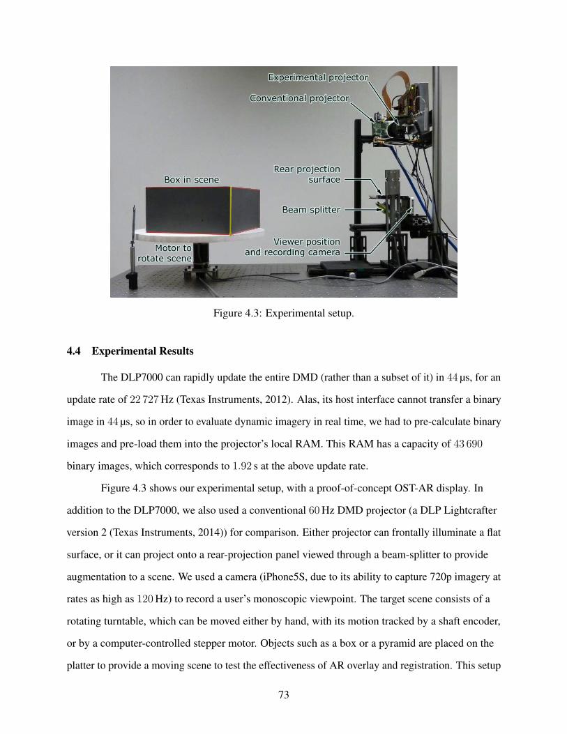
Figure 4.3: Experimental setup.

4.4 Experimental Results

The DLP7000 can rapidly update the entire DMD (rather than a subset of it) in 44 µs, for an

update rate of 22 727Hz (Texas Instruments, 2012). Alas, its host interface cannot transfer a binary

image in 44 µs, so in order to evaluate dynamic imagery in real time, we had to pre-calculate binary

images and pre-load them into the projector’s local RAM. This RAM has a capacity of 43 690

binary images, which corresponds to 1.92 s at the above update rate.

Figure 4.3 shows our experimental setup, with a proof-of-concept OST-AR display. In

addition to the DLP7000, we also used a conventional 60Hz DMD projector (a DLP Lightcrafter

version 2 (Texas Instruments, 2014)) for comparison. Either projector can frontally illuminate a flat

surface, or it can project onto a rear-projection panel viewed through a beam-splitter to provide

augmentation to a scene. We used a camera (iPhone5S, due to its ability to capture 720p imagery at

rates as high as 120Hz) to record a user’s monoscopic viewpoint. The target scene consists of a

rotating turntable, which can be moved either by hand, with its motion tracked by a shaft encoder,

or by a computer-controlled stepper motor. Objects such as a box or a pyramid are placed on the

platter to provide a moving scene to test the effectiveness of AR overlay and registration. This setup

73

(a) Conventional 60Hz color display. Note that the

overlay is displaced significantly from the tip of the

pyramid.

(b) Experimental display at 1 kHz. Without the

need to operate at the maximum rate of 22 727Hz,

1 kHz is enough to show the benefit of using this

low-latency display.

Figure 4.4: AR registration of a moving object (pyramid). These frames were filmed by a 120Hz

camera through a beam splitter (see Figure 4.3).

is analogous to, but simpler to control experimentally than a tracked HMD user. In particular, we

can take advantage of a very-low-latency tracker with controlled, repeatable motion.

4.4.1 Experiment 1: Latency

Our first experiment compared the latency of the conventional 60Hz DMD projector with

that of the low-latency experimental DLP7000. A simple three-axis cursor was positioned in 3D

space at the tip of the physical pyramid model on the turntable. This cursor was rendered for each

projector and for each rotational position of the platter, at intervals of 1/3°. The platter’s position

was tracked by a shaft encoder and the appropriate image was displayed as soon as a shaft encoder

pulse was received. The pulse is input to the DLP7000 via a 1-bit pin; thus only unidirectional

random motion is supported, while there is no such limitation for the conventional projector.

Figure 4.4 shows the results for conventional and experimental projectors as the user rotated the

turntable at a maximum rate of 2/3Hz. As expected, the conventional projector’s image lagged

noticeably behind its intended location at the tip of the pyramid; the experimental projector’s cursor

remained registered.

4.4.2 Experiment 2: Low-Latency Grayscale Imagery Using Binary Image Generation

In the second experiment, we projected a rotating grayscale test pattern (see Figure 4.5 (a))

containing a combination of text, lines, gradients and photos. The resulting set of Binary Projector

Images was displayed at full speed in a continuous 360° loop so the results could be examined

74

(a) Original Test Pattern. Photos

from Wikimedia Commons:

“‘Leaving home’ Statue in

Ningbo” ©Siyuwj; “Client Advi-

sory Team Photo” ©Mshannon,

both CC-BY-SA-3.0 / GFDL.

(b) Projected using a conven-

tional grayscale DMD projector.

Note that the image is generally

sharp within each consecutive

frame, though these two frames

are distinctly visible, which re-

sults in jumpy motion.

(c) Projected using experimental

projector. Note that the center of

the image is sharper while the out-

side edges are more blurred (no

distinct frames are visible), which

results in smooth motion.

Figure 4.5: A frame of the rotating pattern from (a) projected onto a flat surface and captured with

a 120Hz camera, (b), (c). The pattern rotates at a constant rate of 360 °/s.

visually. As expected, the imagery was rotating smoothly, exhibiting increased motion blur near the

edges of the spinning test pattern and very little motion blur near the center. No artifacts were

observed. Figure 4.6 shows a selection of frames from this experiment: Desired Images, Integrated

Perceived Images, Error Images, and Binary Projector Images. Figure 4.5 and the accompanying

video1 show the observed dynamic results.

4.4.3 Experiment 3: AR Imagery on Moving Object

Since our experimental projector requires pre-loaded (and therefore pre-computed) binary

images, the real-life bidirectional motion of the object in this third experiment must be known in

advance. Therefore, instead of moving turntable and object by hand unidirectionally, we moved it

with a PC-controlled stepper motor, through a predefined series of angular positions, in both

directions and at varying speeds. Figure 4.8 shows one such motion profile covering the experiment

pictured in Figure 4.7. The sequence lasted 1.92 s, during which 43 690 binary images were

displayed.

1http://youtu.be/dBFdBm9Ab9E

75

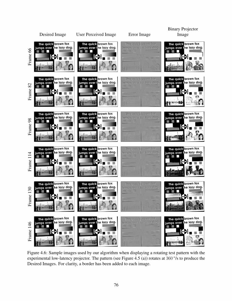
Desired Image User Perceived Image Error Image

Binary Projector

ImageF

ram

e66

Fra

me

82

Fra

me

98

Fra

me

114

Fra

me

130

Fra

me

146

Figure 4.6: Sample images used by our algorithm when displaying a rotating test pattern with the

experimental low-latency projector. The pattern (see Figure 4.5 (a)) rotates at 360 °/s to produce the

Desired Images. For clarity, a border has been added to each image.

76

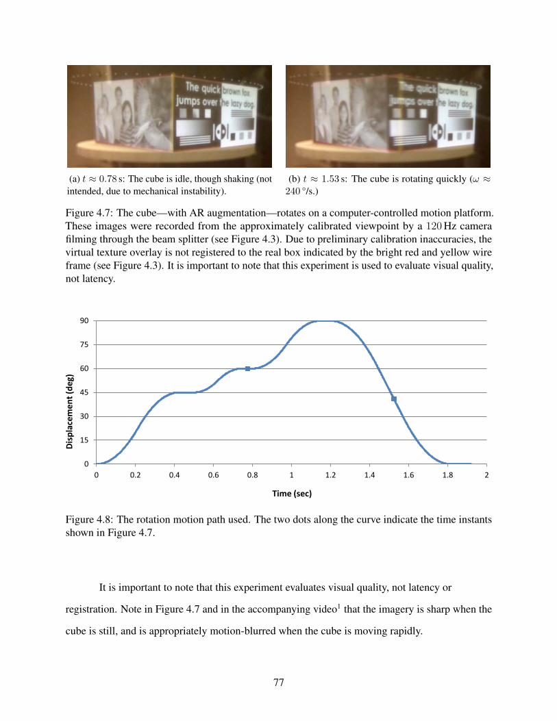
(a) t ≈ 0.78 s: The cube is idle, though shaking (not

intended, due to mechanical instability).

(b) t ≈ 1.53 s: The cube is rotating quickly (ω ≈240 °/s.)

Figure 4.7: The cube—with AR augmentation—rotates on a computer-controlled motion platform.

These images were recorded from the approximately calibrated viewpoint by a 120Hz camera

filming through the beam splitter (see Figure 4.3). Due to preliminary calibration inaccuracies, the

virtual texture overlay is not registered to the real box indicated by the bright red and yellow wire

frame (see Figure 4.3). It is important to note that this experiment is used to evaluate visual quality,

not latency.

0

15

30

45

60

75

90

0 0.2 0.4 0.6 0.8 1 1.2 1.4 1.6 1.8 2

Dis

pla

cem

en

t (d

eg

)

Time (sec)

Figure 4.8: The rotation motion path used. The two dots along the curve indicate the time instants

shown in Figure 4.7.

It is important to note that this experiment evaluates visual quality, not latency or

registration. Note in Figure 4.7 and in the accompanying video1 that the imagery is sharp when the

cube is still, and is appropriately motion-blurred when the cube is moving rapidly.

77

4.5 Conclusion

The proposed low-latency image generation algorithm produces visually pleasing results.

Rapid updates decrease or eliminate the “swimming” artifacts induced by latency, and the imagery

shown by our proposed display is more natural and resembles motion blur, which is more

acceptable to viewers. Without the current hardware’s limitations, we expect even better results

because we could prioritize updates on portions of the display, rather than updating the full binary

DMD array as shown.

We believe that to achieve low-latency in displays, we must abandon full-frame updates,

which necessarily induce excessive latency (unless the update rates are extremely high). This means

that we must also move away from the frame-based legacy display interfaces that are modeled on

decades-old CRT technology.

In addition, the proposed end-to-end low-latency AR pipeline and the low-latency

image-generation algorithm can be readily applied to projector-based SAR and VST-AR, as they

are not tied to optical see-through displays.

4.6 Future Work

We will next focus on developing a real-time display by designing custom hardware to

control the DMD directly, bypassing limitations of the current control hardware. The

implementation will be on a high-performance FPGA, with a high degree of parallelism. Our

Binary Projector Image generation algorithm is easy to parallelize and can be implemented as a

fixed-function pipeline with simple integer math. It requires little memory as it involves only a

small number of most recent projected images and two grayscale images (one integrated Perceived

Image and one Desired Image).

As the bandwidth required to drive the DMD is very high, the control circuitry must be

physically close to the DMD chip. We expect to supply images from a GPU to the controller (in

pairs and with depth, to enable 3D warping (Mark et al., 1997)) over a conventional video interface,

such as DVI (Stoll et al., 2001). Additionally, tracking data must be transmitted. The display

controller should include circuitry to warp the received images (see Figure 4.2) to produce the

78

Desired Images at high rates, as well as to compute the Perceived and Error Images at the same

speeds. This direct rapid control may reduce latency as well as power consumption, and may result

in higher image quality.

Extension to color images, via an approach similar to frame-sequential color, appears

straightforward. We expect the next experimental projector to have three colored light sources, for

instance red, green and blue LEDs. Switching between color channels could occur either at every

update, perhaps every 50 µs, or less frequently if the system were to support mirror changes by

blocks, as expected.

Longer-term plans include investigation of other display types that can be updated rapidly

and are suitable for head-worn displays. Finally, we plan to research approaches to a low-latency

equivalent of a device-independent interface, analogous to HDMI or DisplayPort for conventional

displays. This would be an abstract interface to be used between a device-independent low-latency

renderer and a renderer-independent low-latency display, enabling more of the proposed algorithm

to be implemented in a GPU.

79

CHAPTER 5: FUTURE WORK

There are many future research directions that could be explored beyond the work presented

in this dissertation. Section 5.1 discusses possibilities related to closed-loop registration for

OST-AR, while Section 5.2 presents ideas for combing closed-loop and low-latency registration.

Finally, Section 5.3 presents the idea of designing custom virtual or physical-virtual fiducials for

closed-loop registration in SAR. The custom fiducials can be designed to elicit desirable optical

signals that directly indicate any error in the relative pose between the physical and projected

virtual objects.

5.1 Closed-Loop Optical See-Through AR

In OST-AR, though latency is the most important error source, geometric error sources

alone can result in significant registration errors. Compared to VST-AR and SAR, OST-AR with

optical see-through head-worn displays (OST-HWD) has stricter registration requirements as the

“screen” displaying the virtual imagery is physically much closer to user’s eyes, and the real

imagery moves with no delay. OST-AR system calibration, in particular eye-tracker-display

calibration, is more prone to errors, as user interaction (e.g., point-and-click) is usually required.

This is needed because the system does not know what the user’s eye observes.

Also, due to the lack of retinal access, it is currently impossible to acquire digital

measurements of the output registration. Until an OST-AR system is capable of measuring output

registration as digital images, the methods presented in Chapter 3 cannot be applied. Therefore, to

“close the loop” in the user-perceived augmented imagery in OST-AR, we should include the user in

the loop, ideally without the user knowing it. Previous work by McGarrity et al. (2001) required the

user to indicate the projection of a perceived object on a planar measurement device in order to

quantify registration errors prior to real usage. It may be extended as an online closed-loop

80

approach by using application-embedded interactions, instead of a designated separate task. For

example, an OST-AR application may need to take a user’s finger input for icon selection. We

could overlay the virtual icon onto some real object with known 3D position and measure the offset

between the user’s finger and the icon. In this way, the system can determine the error between

user-perceived icon position (i.e., finger position) and the system-output icon position (i.e., the

underlying real object position). 3D position measurements can be easily acquired using depth

sensors, which are standard equipment in new optical see-through head-worn glasses, e.g.,

SpaceGlasses (Meta, 2014) and HoloLens (Microsoft, 2015).

A more interesting and promising direction in measuring registration imperceptibly or even

densely is using corneal imaging (Nishino and Nayar, 2004b, 2006). A corneal imaging system is a

catadioptric (mirror + lens) imaging system, consisting of the cornea of an eye, which is the

reflector, and a camera viewing the eye. It has been shown that corneal imaging can be used for

gaze estimation (Nakazawa and Nitschke, 2012), display-camera calibration (Nitschke et al.,

2009b,a), environment map computation from a single image (Nishino and Nayar, 2004a) or several

images for super-resolution (Nitschke and Nakazawa, 2012), 3D reconstruction (Nishino and Nayar,

2004b, 2006), and more recently OST-HWD-eye calibration (Plopski et al., 2015). Therefore, we

could use corneal imaging to densely measure the resulting user-observed registration. Additionally,

an OST-HWD with rigidly attached eye-viewing camera(s) could offer several advantages for AR:

1. With the estimated eye gaze, the system has the knowledge of what the real and/or virtual

object the user is viewing at, which is useful for user interaction and registration

refinement towards the specific object (e.g., using the proposed RE-MBT, introduced

in Section 3.2.1.2).

2. With the estimated environment map, which provides the illumination of the real scene

with respect to the eye, the system could perform photometric real-virtual registration, i.e.,

rendering virtual objects consistent with the illumination of the real scene (Nishino and

Nayar, 2004a).

81

3. The OST-HWD, eye(s), and eye-viewing camera(s), could be calibrated together

automatically, by combining automatic display-camera calibration through the camera

(Nitschke et al., 2009b,a) and automatic display-eye calibration through the eye (Itoh and

Klinker, 2014; Plopski et al., 2015).

Another possible direction in registration measurement is through Brain Computer Interface

(BCI). In the visual domain, brain imaging methodologies have revealed a wealth of information

that can be derived from neural processes associated with stimulus presentation. As described

by Lance et al. (2012), neuroimaging techniques can show that the brain is processing visual

information, when that processing is taking place, and can also give insights into the nature of the

processing: where in the visual field a particular stimulus is located, when it was perceived, whether

the stimulus was stationary or moving, whether an image (or mental image of that image) was a

face or a place, and can even provide a partial decoding of a specific image or video. Therefore, we

may be able to detect misregistration-related brain signals or even recover what the user is

observing as digital images.

5.2 Combing Closed-Loop and Low-Latency Registration

Compared to open-loop registration, closed-loop registration may introduce additional

computational delays. For example, in our global-local misregistration minimization method,

model-based tracking and dense optical flow are relatively computationally intensive. Efficient

algorithms can be used to reduce computational delays (Section 3.2.8).

In addition, using faster sensors can help. This can be explained by the relationship between

speed and simplicity described by Bishop (1984):

If the frame rate is fast, consecutive images will be only a little different. Small image

changes can be tracked with a simple algorithm. This simple algorithm can be

implemented with small circuitry. The small circuitry lets a single chip hold the

complete sensor, both imaging and image processing. Such implementation allows

each sensor to be fast because all high-bandwidth communication is done on-chip. The

small size also allows many independent sensors to be placed into the small sensor

82

cluster. This cyclic relationship can spiral up as the design is iterated, wither faster and

simpler operations, or down, with slower and more complex operation.

Though the above describes the cyclic relationship between speed and simplicity for tracking, it can

also be applied to closed-loop registration. With faster sensors, tracking can be easier and more

accurate, hence small registration errors. Small registration errors can be minimized by simpler and

faster closed-loop methods.

Furthermore, closed-loop registration is not necessarily required to run in every frame and

in the same thread or processor as the low-latency registration pipeline. Many structured error

sources, e.g., errors in calibration and modeling, are hard to detect or minimize in a single frame. It

may require several frames to gather enough data. Once these structured registration errors are

minimized they will typically not occur again. Therefore, closed-loop registration could run in a

separate thread or processor, providing delayed adjustments to slowly changing error signals. As a

step further, we could apply closed-loop registration in a fine-grained and just-in-time way, similar

to the proposed end-to-end low-latency pipeline (Figure 4.2). For example, if optical distortion (a

type of calibration errors) in display is detected, we can apply computed adjustments in both the

display (ensure the current image to be displayed is adjusted) and the renderer (ensure all

subsequent images are rendered with counter-distortions to compensate the display distortion).

Finally, we could make registration errors easier to detect and minimize by injecting

artificial signals into virtual and/or real objects, ideally making the error signal self-correcting. In

this way, minimal processing will be needed for closed-loop registration (error detection and

minimization). This method could be useful for projector-based Spatial AR, in which the real

object and the projected virtual object coexist in the same physical space. It is described in detail in

the following section.

5.3 Physical-Virtual Fiducials for Closed-Loop Projector-Based Spatial AR

As a future research direction, I propose to “close the loop” in the displayed appearance in

SAR for both static and dynamic scenes using custom physical-virtual fiducials or only virtual

fiducials. For physical-virtual fiducials, the goal is to design pairs of fiducials comprising (1)

83

Misregistered to the left

Perfectly registered

Misregistered to the right

Misregistered down

Misregistered upMisregistered

to 135⁰ Misregisteredto 45⁰

Misregisteredto 225⁰ Misregistered

to 315⁰

Correction loop

Yellow dot as part of the object (physical fiducial)

Magenta Red

Camera image

(a) (b)

Besides color, we could also use texture, geometry…

Projected magenta dot(virtual fiducial)

Figure 5.1: Conceptual diagram showing using physical and virtual appearance to achieve closed-

loop registration for 2D translational motion in SAR. (a) shows the various components in the

registration feedback-correction loop. Note that a yellow object reflects both red and green light

while it absorbs blue light, and magenta light is a mixture of red light and blue light in equal

intensities. Therefore, if the projected magenta dot is perfectly registered to the yellow physical dot,

the combined dot shows red color. (b) shows the registered and misregistered appearance of the

optical combination of the physical and virtual. It is easy to determine from the combined color

patterns whether and how the physical and virtual are misregistered. Besides color, we could also

use other attributes such as texture and geometry for physical-virtual fiducial design.

physical fiducials affixed directly onto the physical objects and (2) virtual fiducials projected to lie

on top of the physical fiducials such that the combined appearance of the physical and virtual

fiducials provides optical signals that directly indicate error in the relative pose between the

physical and virtual objects. As a step further, using only custom virtual fiducials which adapt to

physical attributes of real objects can also produce similar misregistration-responsive and

-correcting optical signal. This optical error signal could be comprised of geometry (e.g., curvature,

volume, and area) and/or surface characteristics (e.g., color, texture, and BRDF) in easily

identifiable patterns. With the use of such fiducials, SAR systems can be capable of automatically

and continuously sensing and minimizing registration errors.

84

Figure 5.2: Target under different lighting directions. Source: Matusik et al. (2009).

5.3.1 Error Signal Appearance

We use camera as the sensor for closed-loop registration. As a result, the appearance of

registration error signals is comprised of intensity and color values. We could design

physical-virtual fiducials to show error signals of specific intensity or color values for different

6DOF pose errors. Such error signals can be directly read out with minimal image processing. The

Agam fiducial (Bruckstein et al., 2000) uses intensity as immediate and unique labeling of the

viewing direction. Figure 5.1 shows a simple conceptual example of physical-virtual fiducials using

color as the error signal. In addition, error signals using intensity or color can be measured by

sensors other than cameras, such as photometers and RGB color sensors.

Error signals could use attributes other than intensity and color, such as gradient, frequency

and even reflectance effects. For example, Tanaka et al. (2012) used black bars in moire patterns to

determine out-of-plane rotations. Figure 5.2 shows an object surface having spatially-varying

BRDF that gives different reflectance effects under different light directions (Matusik et al., 2009).

5.3.2 Physical-Virtual Fiducial Design

The goal is to design physical-virtual fiducials to exhibit desirable optical error signals that

directly indicate the error in the relative 6DOF pose between the physical and projected virtual

objects. And the fiducials should cause minimal degradation to the final user imagery and become

imperceptible when registered.

To design such fiducials, we need to identify parameters that define the appearance of

physical-virtual fiducials, as well as design constraints. Then we can build an optimizer to produce

85

Parameter space

Geometry

Curvature

Volume

Area

Surface

Color Texture

Frequency

Gradient

Reflectance

Diffuse

Specular

BRDF

Material

Transparency

Translucency

…

…

Figure 5.3: Parameter space for designing physical-virtual fiducials.

physical-virtual fiducials with desirable properties, considering both adjustable parameters and

constraints.

5.3.2.1 Parameter Space

The appearance of physical and virtual fiducials is determined by their geometry and

surface properties.

• Geometry properties include but not limited to curvature, volume and area. They

describe the shape of a physical or virtual fiducial. The fiducial can be planar or

non-planar, and smooth or non-smooth, e.g., sphere, cube, or prism.

• Surface properties include but not limited to color, texture, reflectance and material.

Color describes the light absorbency properties of an object. Texture describes the spatial

variation on an object surface. Reflectance describes the fraction of incident radiation

reflected by a surface, e.g., diffuse, specular, or BRDF in general. Material attributes

86

include transparency and translucency, describing the physical property of allowing light

to pass through the object.

These properties are summarized in Figure 5.3, forming the parameter space for designing

physical-virtual fiducials.

5.3.2.2 Design Constraints

Constraints on designing physical-virtual fiducials are specified as follows:

• Responsiveness. The fiducials should give an obvious error signal to the system when the

real and virtual are misregistered.

• Imperceptibility. The fiducials should give no error signal when the real and virtual are

registered.

• Uniqueness. The error signal should relate to the pose error as a one-to-one mapping, i.e.,

from one error signal, we can uniquely tell the corresponding pose error, and vice versa.

• Complexity. The error signal should require minimal computational load to detect and

correct in order to run in real-time.

Mathematically, the error signal can be simply expressed as:

E(p) = R(pr) mod V (pv) (5.1)

p = pr − pv (5.2)

and some expressible constraints are

E(p) 6= 0, if p 6= 0 (Responsiveness constraint) (5.3)

E(p) = 0, if p = 0 (Imperceptibility constraint) (5.4)

f : p→ E and f−1 : E → p (Uniqueness constraint) (5.5)

87

Geometry parameters

Surface parameters

Optimizer

Constraints on error signal:

responsiveness uniqueness…

Physical fiducial

Virtual fiducial

Curvature

Volume

Edge

……

…

Color

Texture

Material

……

…

Figure 5.4: Optimization framework for designing physical-virtual fiducial pairs and custom virtual

fiducials.

where E denotes the optically combined error signal measured by some sensor, R is the physical

fiducial/signal, V is the virtual fiducial/signal, and mod is the modulation operator representing the

modulation between the projector light and object surface; pr and pv are vectors denoting 6DOF

pose of the physical and virtual respectively, and p is the difference of pr and pv, i.e., the relative

pose error.

5.3.2.3 Optimization Setup

Driven by the constraints of the error signal, we can then optimize for the geometry and

surface parameters of the fiducials. The optimization scheme is shown in Figure 5.4. Geometry and

surface parameters are input to the optimizer, which produces pairs of physical-virtual fiducials as

output. For custom virtual fiducials, useful natural attributes of physical objects need to be first

extracted and then fed to the optimizer as input to determine the optimal parameters of the

corresponding virtual fiducial. The design of the optimizer is the main challenge due to strict

constraints and to the large degrees of freedom in both the parameter space and the solution space.

It remains to be explored what the optimizer is.

88

CHAPTER 6: CONCLUSION

This thesis is motivated by “the last mile” of registration in AR, which refers to the delivery

of spatially and temporally registered augmented imagery to the end user. Results of this thesis

work show that “the last mile” can benefit greatly from both fine-grained render-display processing

and closed-loop real-virtual adaptation. Let us review the major points and contributions presented

in this dissertation.

6.1 Closed-Loop Spatial Registration

In Chapter 3, I presented closed-loop spatial registration for minimizing registration errors

caused by geometric errors, i.e., errors in calibration, tracking, and modeling. A global-local

closed-loop registration framework is introduced for minimizing both rigid and nonrigid registration

errors using a reference model composed of a model of the real scene and the desired virtual

augmentations. Registration errors are minimized in both global world space via camera pose

refinement, and local screen space via pixel-wise corrections, resulting in pixel-accurate registration.

Contribution 1. For projector-based Spatial AR, I proposed model-based registration

(MBR) as a global closed-loop registration method. It combines tracking and augmentation for the

purpose of registration in a more compact closed-loop framework without using an extra step for

correction. I also presented a simple but effective method for extending MBR to video see-through

AR (VST-AR), named E-MBR, by digitally simulating the “projection” using linear image

operations. It has been experimentally proved that E-MBR achieves better registration accuracy

compared to a popular open-loop approach.

Contribution 2. For VST-AR, I proposed both global world-space and local screen-space

misregistration minimization methods, which are integrated into an effective closed-loop

registration framework. While E-MBR is proved to be mathematically equivalent to the

89

conventional model-based tracking (MBT) for pose refinement, it can be used as a good

visualization tool for showing the iterative registration error minimization process. The major

drawback of E-MBR and MBT is that they minimize pose errors rather than registration errors,

which is harmful when the model being used is wrong. To cope with that, I proposed

registration-enforcing model-based tracking (RE-MBT) which incorporates the important

real-virtual association information—that is, we typically know, as prior information, which real

object in the scene the virtual object should be registered to. With the use of the real-virtual

association information, RE-MBT can guide pose refinement towards better registration, even in the

presence of rigid modeling errors.

Contribution 3. As a subsequent step after pose refinement, I introduced local

screen-space registration correction in order to deal with the remaining errors, which can be rigid

(e.g., uncorrected pose errors) or nonrigid (e.g., radial distortion). It works by computing the

per-pixel displacement (i.e., optical flow) between the camera image and the model image rendered

with the refined pose, and using the per-pixel displacement field to directly correct misregistration

in screen space. The “screen space” can be equivalent to the real camera image space

(forward-warping augmented reality, or FW-AR) or the virtual camera image space

(backward-warping augmented virtuality, or BW-AV).

Our closed-loop approaches for SAR and VST-AR are optimal for visual registration as we

minimize a cost function of misregistration. The stability is also guaranteed if the cost function is

minimized.

6.2 Low-Latency Temporal Registration

In Chapter 4, I presented low-latency temporal registration for minimizing temporal

registration errors caused by system latency. I introduced a low-latency rendering pipeline which

employs a cascade of successively simpler and faster renderers. Each renderer can respond to the

latest tracking data. This approach is motivated by just-in-time rendering (Section 2.3.2.2).

Contribution 4. The major contribution in this chapter was a new image generation

approach for low-latency displays such as those needed in head-worn AR devices. The new

90

approach has been demonstrated with a bench-top OST-AR proof-of-concept prototype that uses

DLP™ DMD projector. It has been shown that a perceptually-continuous-tone dynamic gray-scale

image can be efficiently composed from a very rapid succession of binary (partial) images, each

calculated from the continuous-tone image generated with the most recent tracking data. As the

DMD projects only a binary image at any moment, it cannot instantly display this latest

continuous-tone image, and conventional decomposition of a continuous-tone image into binary

time-division-multiplexed values would induce just the latency we seek to avoid. Instead, the

proposed approach maintains an estimate of the image the user currently perceives, and at every

opportunity allowed by the control circuitry, sets each binary DMD pixel to the value that will

reduce the difference between that user-perceived image and the newly generated image from the

latest tracking data. This approach allows a DMD projector to display grayscale images at its

internally maximum switching rate, reducing the latency in DMD projectors to the minimum. The

resulting displayed binary image is “neither here nor there,” but always approaches the moving

target that is the constantly changing desired image, even when that image changes every 50 µs. We

have compared our experimental results to imagery from a conventional DLP projector with similar

internal speeds, and have demonstrated that AR overlays on a moving object are more effective

with this kind of low-latency display device than with displays of a similar speed that use a

conventional video interface.

6.3 Future Possibilities

In Chapter 5, I introduced several future directions that could be explored beyond the work

presented in this dissertation. One important direction is to “close the loop” in the user-perceived

augmented imagery in OST-AR. To cope with the problem of registration measurement in OST-AR

due to the lack of retinal access, we could imperceptibly include the user in the loop by using

application-embedded interactions for sparse misregistration quantification, or corneal imaging or

even brain imaging for dense recovery of the augmented imagery.

Another important direction is to combine closed-loop spatial registration and low-latency

temporal registration. The computational delay introduced by closed-loop registration (registration

91

sensing, error detection and minimization) could be reduced by using efficient algorithms as well as

faster sensors. We could also decouple closed-loop and low-latency registration by making the

closed-loop process run in another thread or processor, providing delayed adjustments to slowly

changing error signals. When any registration adjustment is computed, it could be applied in a

fine-grained and just-in-time way.

Lastly, I presented the idea of designing custom virtual or physical-virtual fiducials for

closed-loop registration in SAR. This idea is a new paradigm where one “injects signal” by using

fiducials (or more generally custom real-world objects) that directly convey registration errors.

Such direct error signals could be detected and corrected with minimal latency.

92

REFERENCES

Adelstein, B. D., Jung, J. Y., and Ellis, S. R. (2001). Predictive Compensator Optimization for

Head Tracking Lag in Virtual Environments. National Aeronautics and Space Administration,

Ames Research Center.

Adelstein, B. D., Lee, T. G., and Ellis, S. R. (2003). Head Tracking Latency in Virtual

Environments: Psychophysics and a Model. In Proc. 47th Annual Meeting of the Human

Factors and Ergonomics Society, pages 2083–2087, Santa Monica, CA.

Akatsuka, Y. and Bekey, G. A. (1998). Compensation for end to end delays in a vr system. In

Proceedings IEEE Virtual Reality Annual International Symposium, pages 156–159.

Allen, B. D., Bishop, G., and Welch, G. (2001). Tracking: Beyond 15 Minutes of Thought:

SIGGRAPH 2001 Course 11. SIGGRAPH Course Pack edition.

Allison, R., Harris, L., Jenkin, M., Jasiobedzka, U., and Zacher, J. (2001). Tolerance of temporal

delay in virtual environments. In Proc. IEEE Virtual Reality (VR), pages 247–254.

AMD (2014). Amd freesync technology. http://www.amd.com/en-us/innovations/

software-technologies/technologies-gaming/freesync.

Amin, M. S., Konrad, H., and Konrad, H. (2012). Vestibuloocular reflex testing.

http://emedicine.medscape.com/article/1836134-overview.

Armstrong, M. and Zisserman, A. (1995). Robust object tracking. In Proc. Asian Conference on

Computer Vision.

Audet, S. and Okutomi, M. (2009). A user-friendly method to geometrically calibrate

projector-camera systems. Computer Vision and Pattern Recognition Workshop, 0:47–54.

Audet, S., Okutomi, M., and Tanaka, M. (2010). Direct image alignment of projector-camera

systems with planar surfaces. In Computer Vision and Pattern Recognition (CVPR), 2010

IEEE Conference on, pages 303 –310.

Azuma, R., Baillot, Y., Behringer, R., Feiner, S., Julier, S., and MacIntyre, B. (2001). Recent

advances in augmented reality. IEEE Computer Graphics and Applications, 21(6):34–47.

Azuma, R. and Bishop, G. (1994). Improving static and dynamic registration in an optical

see-through hmd. In Proceedings of the 21st annual conference on Computer graphics and

interactive techniques, SIGGRAPH ’94, pages 197–204, New York, NY, USA. ACM.

Azuma, R. and Bishop, G. (1995). A Frequency-Domain Analysis of Head-motion Prediction. In

Proceedings of the 22nd Annual Conference on Computer Graphics and Interactive

Techniques (SIGGRAPH), SIGGRAPH ’95, pages 401–408, New York, NY, USA. ACM.

Azuma, R. T. (1995). Predictive Tracking for Augmented Reality. PhD thesis, University of North

Carolina at Chapel Hill.

93

Azuma, R. T. (1997). A Survey of Augmented Reality. Presence: Teleoperators and Virtual

Environments, 6(4):355–385.

Azuma, R. T., Hoff, B. R., Neely, III, H. E., Sarfaty, R., Daily, M. J., Bishop, G., Vicci, L., Welch,

G., Neumann, U., You, S., Nichols, R., and Cannon, J. (1999). Making augmented reality

work outdoors requires hybrid tracking. In Proceedings of the International Workshop on

Augmented Reality : Placing Artificial Objects in Real Scenes: Placing Artificial Objects in

Real Scenes, IWAR ’98, pages 219–224, Natick, MA, USA. A. K. Peters, Ltd.

Bailey, R. E., Arthur III, J. J., and Williams, S. P. (2004). Latency Requirements for Head-Worn

Display S/EVS Applications. In Proc. SPIE, volume 5424, pages 98–109.

Bajura, M. and Neumann, U. (1995). Dynamic registration correction in video-based augmented

reality systems. IEEE Comput. Graph. Appl., 15(5):52–60.

Baker, S. and Matthews, I. (2001). Equivalence and efficiency of image alignment algorithms. In

Computer Vision and Pattern Recognition, 2001. CVPR 2001. Proceedings of the 2001 IEEE

Computer Society Conference on, volume 1, pages I–1090–I–1097 vol.1.

Baker, S. and Matthews, I. (2004). Lucas-kanade 20 years on: A unifying framework. Int. J.

Comput. Vision, 56(3):221–255.

Bandyopadhyay, D., Raskar, R., and Fuchs, H. (2001). Dynamic Shader Lamps : Painting on

Movable Objects. In Augmented Reality, 2001. Proceedings. IEEE and ACM International

Symposium on, pages 207–216.

Bartoli, A. (2008). Groupwise Geometric and Photometric Direct Image Registration. IEEE Trans.

Pattern Anal. Mach. Intell., 30(12):2098–2108.

Benhimane, S. and Malis, E. (2004). Real-time image-based tracking of planes using efficient

second-order minimization. In Intelligent Robots and Systems, 2004. (IROS 2004).

Proceedings. 2004 IEEE/RSJ International Conference on, volume 1, pages 943–948 vol.1.

Benhimane, S. and Malis, E. (2007). Homography-based 2d visual tracking and servoing. Int. J.

Rob. Res., 26(7):661–676.

Bhatnagar, D. K. (1993). Position Trackers for Head Mounted Display Systems: A Survey.

Technical report, University of North Carolina at Chapel Hill.

Bimber, O. and Raskar, R. (2005). Spatial Augmented Reality: Merging Real and Virtual Worlds.

A. K. Peters, Ltd., Natick, MA, USA.

Bishop, G. (1984). Self-tracker: A Smart Optical Sensor on Silicon. PhD thesis, University of

North Carolina at Chapel Hill. AAI8415794.

Bishop, G., Fuchs, H., McMillan, L., and Zagier, E. J. S. (1994). Frameless rendering: Double

buffering considered harmful. In Proc. of the 21st Annual Conference on Computer Graphics

and Interactive Techniques, SIGGRAPH ’94, pages 175–176, New York, NY, USA. ACM.

94

Bleser, G., Wuest, H., and Strieker, D. (2006). Online Camera Pose Estimation in Partially Known

and Dynamic Scenes. In Proc. ISMAR 2006, pages 56–65.

Bruckstein, A. M., Holt, R. J., Huang, T. S., and Netravali, A. N. (2000). New devices for 3d pose

estimation: Mantis eyes, agam paintings, sundials, and other space fiducials. International

Journal of Computer Vision, 39:131–139. 10.1023/A:1008123110489.

Buker, T. J., Vincenzi, D. A., and Deaton, J. E. (2012). The Effect of Apparent Latency on

Simulator Sickness While Using a See-Through Helmet-Mounted Display: Reducing

Apparent Latency With Predictive Compensation. Human Factors: The Journal of the Human

Factors and Ergonomics Society, 54(2):235–249.

Caudell, T. and Mizell, D. (1992). Augmented reality: an application of heads-up display

technology to manual manufacturing processes. In System Sciences, 1992. Proceedings of the

Twenty-Fifth Hawaii International Conference on, volume ii, pages 659 –669 vol.2.

Chaumette, F. and Hutchinson, S. (2006). Visual Servo Control Part I: Basic Approaches. IEEE

Robotics Automation Magazine, 13(4):82–90.

Chaumette, F. and Hutchinson, S. (2007). Visual Servo Control Part II: Advanced Approaches.

IEEE Robotics Automation Magazine, 14(1):109–118.

Comport, A., Marchand, E., Pressigout, M., and Chaumette, F. (2006). Real-Time Markerless

Tracking for Augmented Reality: The Virtual Visual Servoing Framework. IEEE Transactions

on Visualization and Computer Graphics (TVCG), 12(4):615–628.

Daponte, P., Vito, L. D., Picariello, F., and Riccio, M. (2014). State of the art and future

developments of the augmented reality for measurement applications. Measurement, 57(0):53 –

70.

Davison, A., Mayol, W., and Murray, D. (2003). Real-time localization and mapping with wearable

active vision. In Mixed and Augmented Reality, 2003. Proceedings. The Second IEEE and

ACM International Symposium on, pages 18–27.

Dayal, A., Woolley, C., Watson, B., and Luebke, D. (2005). Adaptive Frameless Rendering. In

Proc. Eurographics Conference on Rendering Techniques, pages 265–275.

Debevec, P. (1998). Rendering Synthetic Objects into Real Scenes: Bridging Traditional and

Image-based Graphics with Global Illumination and High Dynamic Range Photography. In

Proc. SIGGRAPH 1998, pages 189–198.

Dedual, N. J., Oda, O., and Feiner, S. K. (2011). Creating Hybrid User Interfaces with a 2D

Multi-touch Tabletop and a 3D See-Through Head-Worn Display. In Proc. ISMAR 2011,

pages 231–232.

Didier, J., Roussel, D., and Mallem, M. (2005). A Time Delay Compensation Method Improving

Registration for Augmented Reality . In 2005 IEEE International Conference on Robotics and

Automation (ICRA 2005), pages 3396–3400, Barcelona (Spain).

95

DiVerdi, S. and Hollerer, T. (2006). Image-space Correction of AR Registration Errors Using

Graphics Hardware. In Proc. IEEE Virtual Reality (VR’06), pages 241–244.

Drummond, T. and Cipolla, R. (2002). Real-time visual tracking of complex structures. Pattern

Analysis and Machine Intelligence, IEEE Transactions on, 24(7):932–946.

Ellis, S. R., Adelstein, B. D., Mania, K., and Hill, M. I. (2004). Generalizeability of latency

detection in a variety of virtual environments. In Proc. 48th Annual Meeting of the Human

Factors and Ergonomics Society, page 20832087.

Epson (2014). Epson Moverio BT-200 User’s Guide.

https://files.support.epson.com/docid/cpd4/cpd40542.pdf.

Feiner, S., MacIntyre, B., Hollerer, T., and Webster, A. (1997). A touring machine: Prototyping 3d

mobile augmented reality systems for exploring the urban environment. In Proceedings of the

1st IEEE International Symposium on Wearable Computers, ISWC ’97, pages 74–,

Washington, DC, USA. IEEE Computer Society.

Feiner, S., Macintyre, B., and Seligmann, D. (1993). Knowledge-based augmented reality.

Commun. ACM, 36(7):53–62.

Fiala, M. (2005). Artag, a fiducial marker system using digital techniques. In Computer Vision and

Pattern Recognition, 2005. CVPR 2005. IEEE Computer Society Conference on, volume 2,

pages 590 – 596 vol. 2.

Fiala, M. (2010). Designing highly reliable fiducial markers. Pattern Analysis and Machine

Intelligence, IEEE Transactions on, 32(7):1317–1324.

Fuchs, H., Livingston, M. A., Raskar, R., State, A., Crawford, J. R., Rademacher, P., Drake, S. H.,

and Meyer, A. A. (1998). Augmented reality visualization for laparoscopic surgery. In

Proceedings of the First International Conference on Medical Image Computing and

Computer-Assisted Intervention, pages 934–943. Springer-Verlag.

Gruber, L., Gauglitz, S., Ventura, J., Zollmann, S., Huber, M., Schlegel, M., Klinker, G.,

Schmalstieg, D., and Tobias Hollerer (2010). The City of Sights: Design, Construction, and

Measurement of an Augmented Reality Stage Set. In Proc. ISMAR 2010, pages 157–163.

Harders, M., Bianchi, G., Knoerlein, B., and Szekely, G. (2009). Calibration, Registration, and

Synchronization for High Precision Augmented Reality Haptics. IEEE Transactions on

Visualization and Computer Graphics (TVCG), 15(1):138–149.

Harris, C. and Stennett, C. (1990). RAPID - A Video Rate Object Tracker. In Proc. British

Machine Vision Conference (BMVC’90), pages 73–78.

Harris, C. and Stephens, M. (1988). A combined corner and edge detector. In Proceedings of the

4th Alvey Vision Conference, pages 147–151.

Herout, A., Szentandrasi, I., Zacharia, M., Dubska, M., and Kajan, R. (2013). Five Shades of Grey

for Fast and Reliable Camera Pose Estimation. In IEEE Conference on Computer Vision and

Pattern Recognition (CVPR 2013), pages 1384–1390.

96

Hill, M. I., Adelstein, B. D., and Ellis, S. R. (2004). Achieving minimum latency in virtual

environment applications. In IMAGE Society Annual Conference, Scottsdale, AZ.

Hilliges, O., Kim, D., Izadi, S., Weiss, M., and Wilson, A. (2012). Holodesk: Direct 3d interactions

with a situated see-through display. In Proceedings of the SIGCHI Conference on Human

Factors in Computing Systems (CHI’12), CHI ’12, pages 2421–2430, New York, NY, USA.

ACM.

Himberg, H. and Motai, Y. (2009). Head Orientation Prediction: Delta Quaternions Versus

Quaternions. IEEE Transactions on Systems, Man, and Cybernetics, Part B: Cybernetics,,

39(6):1382–1392.

Holloway, R. L. (1997a). Registration Error Analysis for Augmented Reality. Presence:

Teleoperators and Virtual Environments, 6(4):413–432.

Holloway, R. L. (1997b). Registration Error Analysis for Augmented Reality. PhD thesis,

University of North Carolina at Chapel Hill.

Horn, B. K. P. and Schunk, B. G. (1981). Determining Optical Flow. Artificial Intelligence,

17:185–203.

Itoh, Y. and Klinker, G. (2014). Interaction-free calibration for optical see-through head-mounted

displays based on 3D eye localization. In IEEE Symposium on 3D User Interfaces, 3DUI 2014,

Minneapolis, MN, USA, March 29-30, 2014, pages 75–82.

Jacobs, M. C., Livingston, M. A., and State, A. (1997). Managing latency in complex augmented

reality systems. In Proceedings of the 1997 symposium on Interactive 3D graphics, I3D ’97,

pages 49–ff., New York, NY, USA. ACM.

Jerald, J., Fuller, A., Lastra, A., Whitton, M., Kohli, L., and Brooks, F. (2007). Latency

compensation by horizontal scanline selection for head- mounted displays. In Proc. SPIE,

Stereoscopic Displays and Virtual Reality Systems, volume 6490, pages 64901Q–64901Q–11.

Jerald, J. and Whitton, M. (2009). Relating Scene-Motion Thresholds to Latency Thresholds for

Head-Mounted Displays. In Proc. IEEE Virtual Reality, pages 211–218.

Jerald, J. J. (2009). Scene-Motion- and Latency-Perception Thresholds for Head-Mounted Displays.

PhD thesis, University of North Carolina at Chapel Hill.

Jones, A., Lang, M., Fyffe, G., Yu, X., Busch, J., McDowall, I., Bolas, M., and Debevec, P. (2009).

Achieving Eye Contact in a One-to-Many 3D Video Teleconferencing System. ACM Trans.

Graph.

Jones, B. R., Benko, H., Ofek, E., and Wilson, A. D. (2013). Illumiroom: Peripheral projected

illusions for interactive experiences. In Proceedings of the SIGCHI Conference on Human

Factors in Computing Systems, CHI ’13, pages 869–878, New York, NY, USA. ACM.

Jota, R., Ng, A., Dietz, P., and Wigdor, D. (2013). How Fast is Fast Enough?: A Study of the

Effects of Latency in Direct-touch Pointing Tasks. In Proc. ACM CHI, pages 2291–2300.

97

Julier, S. and La Viola, J.J., J. (2004). An Empirical Study into the Robustness of Split Covariance

Addition (SCA) for Human Motion Tracking. In Proceedings of the 2004 American Control

Conference, volume 3, pages 2190–2195 vol.3.

Kato, H. and Billinghurst, M. (1999). Marker Tracking and HMD Calibration for a Video-Based

Augmented Reality Conferencing System. In Proceedings of the 2nd IEEE and ACM

International Workshop on Augmented Reality, IWAR ’99, pages 85–, Washington, DC, USA.

IEEE Computer Society.

Kijima, R. and Ojika, T. (2002). Reflex HMD to Compensate Lag and Correction of Derivative

Deformation. In Proc. IEEE Virtual Reality, pages 172–179.

Kim, K., Lepetit, V., and Woo, W. (2012). Real-time interactive modeling and scalable multiple

object tracking for {AR}. Computers & Graphics, 36(8):945 – 954. Graphics Interaction

Virtual Environments and Applications 2012.

Klein, G. and Drummond, T. (2003). Robust Visual Tracking for Non-Instrumented Augmented

Reality. In Proc. ISMAR 2003, pages 113–122.

Klein, G. and Drummond, T. (2004). Sensor Fusion and Occlusion Refinement for Tablet-based

AR. In Proc. ISMAR 2004, pages 38–47.

Klein, G. and Murray, D. (2007). Parallel Tracking and Mapping for Small AR Workspaces. In

Proc. ISMAR 2007.

Knecht, M., Traxler, C., Purgathofer, W., and Wimmer, M. (2011). Adaptive Camera-based Color

Mapping for Mixed-Reality Applications. In Proc. ISMAR 2011, pages 165–168.

Lance, B., Kerick, S., Ries, A., Oie, K., and McDowell, K. (2012). Brain computer interface

technologies in the coming decades. Proceedings of the IEEE, 100(Special Centennial

Issue):1585–1599.

LaViola, J. J. (2003a). A Testbed for Studying and Choosing Predictive Tracking Algorithms in

Virtual Environments. In Proceedings of the Workshop on Virtual Environments (EGVE ’03),

EGVE ’03, pages 189–198, New York, NY, USA. ACM.

LaViola, J. J. (2003b). Double Exponential Smoothing: An Alternative to Kalman Filter-based

Predictive Tracking. In Proceedings of the Workshop on Virtual Environments (EGVE ’03),

EGVE ’03, pages 199–206, New York, NY, USA. ACM.

Lepetit, V. and Fua, P. (2005). Monocular model-based 3d tracking of rigid objects. Found. Trends.

Comput. Graph. Vis., 1(1):1–89.

Li, H., Roivainen, P., and Forcheimer, R. (1993). 3D Motion Estimation in Model-Based Facial

Image Coding. IEEE Trans. Pattern Anal. Mach. Intell., 15(6):545–555.

Lieberknecht, S., Benhimane, S., Meier, P., and Navab, N. (2009). A dataset and evaluation

methodology for template-based tracking algorithms. In Proceedings of the 2009 8th IEEE

International Symposium on Mixed and Augmented Reality, ISMAR ’09, pages 145–151,

Washington, DC, USA. IEEE Computer Society.

98

Lowe, D. (2004). Distinctive image features from scale-invariant keypoints. International Journal

of Computer Vision, 60(2):91–110.

Lucas, B. D. and Kanade, T. (1981). An iterative image registration technique with an application

to stereo vision. In Proceedings of the 7th International Joint Conference on Artificial

Intelligence - Volume 2, IJCAI’81, pages 674–679, San Francisco, CA, USA. Morgan

Kaufmann Publishers Inc.

Luckey, P. (2013). Building a sensor for low latency virtual reality — Oculus Rift - virtual reality

headset for 3d gaming. http:

//www.oculusvr.com/blog/building-a-sensor-for-low-latency-vr/.

Ma, Y., Soatto, S., Kosecka, J., and Sastry, S. S. (2003). An Invitation to 3-D Vision. Springer.

MacIntyre, B. and Julier, S. J. (2002). Estimating and Adapting to Registration Errors in

Augmented Reality Systems. In Proc. IEEE Virtual Reality (VR’02), pages 73–80.

MacIntyre, B. and M. Coelho, E. (2000). Adapting to Dynamic Registration Errors Using Level of

Error (LOE) Filtering. In Proceedings IEEE and ACM International Symposium on

Augmented Reality, 2000 (ISAR 2000)., pages 85 –88.

Maimone, A., Lanman, D., Rathinavel, K., Keller, K., Luebke, D., and Fuchs, H. (2014). Pinlight

Displays: Wide Field of View Augmented Reality Eyeglasses Using Defocused Point Light

Sources. ACM Trans. Graph., 33(4):89:1–89:11.

Mania, K., Adelstein, B. D., Ellis, S. R., and Hill, M. I. (2004). Perceptual Sensitivity to Head

Tracking Latency in Virtual Environments with Varying Degrees of Scene Complexity. In

Proceedings of the 1st Symposium on Applied Perception in Graphics and Visualization,

APGV ’04, pages 39–47, New York, NY, USA. ACM.

Mark, W. R., McMillan, L., and Bishop, G. (1997). Post-Rendering 3D Warping. In Proceedings of

the 1997 Symposium on Interactive 3D Graphics, I3D ’97, pages 7–ff., New York, NY, USA.

ACM.

Matusik, W., Ajdin, B., Gu, J., Lawrence, J., Lensch, H. P. A., Pellacini, F., and Rusinkiewicz, S.

(2009). Printing spatially-varying reflectance. ACM Trans. Graph., 28(5):128:1–128:9.

McDowall, I. and Bolas, M. (2005). Fast Light for Display, Sensing and Control Applications. In

IEEE VR Workshop on Emerging Display Technologies.

McGarrity, E., Genc, Y., Tuceryan, M., Owen, C., and Navab, N. (2001). A New System for Online

Quantitative Evaluation of Optical See-Throughh Augmentation. In Augmented Reality, 2001.

Proceedings. IEEE and ACM International Symposium on, pages 157–166.

McMillan, L. and Bishop, G. (1995). Plenoptic Modeling: An Image-based Rendering System. In

Proceedings of the 22Nd Annual Conference on Computer Graphics and Interactive

Techniques, SIGGRAPH ’95, pages 39–46, New York, NY, USA. ACM.

99

Meehan, M., Razzaque, S., Whitton, M. C., and Brooks, Jr., F. P. (2003). Effect of Latency on

Presence in Stressful Virtual Environments. In Proceedings of the IEEE Virtual Reality (VR),

VR ’03, pages 141–, Washington, DC, USA. IEEE Computer Society.

Meilland, M., Barat, C., and Comport, A. (2013). 3d high dynamic range dense visual slam and its

application to real-time object re-lighting. In Mixed and Augmented Reality (ISMAR), 2013

IEEE International Symposium on, pages 143–152.

Menozzi, A., Clipp, B., Wenger, E., Heinly, J., Towles, H., Frahm, J.-M., and Welch, G. (2014).

Development of Vision-aided Navigation for a Wearable Outdoor Augmented Reality System.

In Proc. IEEE/ION Position Location and Navigation Symposium, volume (in press).

Meta (2014). Spaceglasses. https://www.spaceglasses.com/.

Meyer, K., Applewhite, H., and Biocca, F. (1992). A Survey of Position Trackers. Presence:

Teleoperators and Virtual Environments, 1(2):173–200.

Microsoft (2015). Hololens. http://www.microsoft.com/microsoft-hololens/en-us.

Milgram, P., Takemura, H., Utsumi, A., and Kishino, F. (1995). Augmented Reality: A Class of

Displays on the Reality-Virtuality Continuum. In SPIE, volume 2351, pages 282–292.

Mine, M. and Bishop, G. (1993). Just-In-Time Pixels. Technical report, University of North

Carolina at Chapel Hill.

Mohan, A., Woo, G., Hiura, S., Smithwick, Q., and Raskar, R. (2009). Bokode: imperceptible

visual tags for camera based interaction from a distance. ACM Trans. Graph., 28(3):98:1–98:8.

Naimark, L. and Foxlin, E. (2002). Circular data matrix fiducial system and robust image

processing for a wearable vision-inertial self-tracker.

Nakazawa, A. and Nitschke, C. (2012). Point of gaze estimation through corneal surface reflection

in an active illumination environment. In Fitzgibbon, A., Lazebnik, S., Perona, P., Sato, Y.,

and Schmid, C., editors, Computer Vision – ECCV 2012, Lecture Notes in Computer Science,

pages 159–172. Springer Berlin Heidelberg.

Neumann, U. and Fuchs, H. (1993). A vision of telepresence for medical consultations and other

applications. In Proceedings of the Sixth International Symposium on Robotics Research,

pages 565–571.

Newcombe, R., Lovegrove, S., and Davison, A. (2011a). DTAM: Dense tracking and mapping in

real-time. In Proc. IEEE Int’l Conf. on Computer Vision, pages 2320 –2327.

Newcombe, R. A., Izadi, S., Hilliges, O., Molyneaux, D., Kim, D., Davison, A. J., Kohi, P., Shotton,

J., Hodges, S., and Fitzgibbon, A. (2011b). Kinectfusion: Real-time dense surface mapping

and tracking. In Mixed and Augmented Reality (ISMAR), 2011 10th IEEE International

Symposium on, pages 127–136.

Ng, A., Lepinski, J., Wigdor, D., Sanders, S., and Dietz, P. (2012). Designing for Low-latency

Direct-touch Input. In Proc. ACM UIST, pages 453–464.

100

Nishino, K. and Nayar, S. (2004a). Eyes for Relighting. ACM Transactions on Graphics (also Proc.

of SIGGRAPH), 23(3):704–711.

Nishino, K. and Nayar, S. (2004b). The World in an Eye. In IEEE Conference on Computer Vision

and Pattern Recognition (CVPR), volume I, pages 444–451.

Nishino, K. and Nayar, S. K. (2006). Corneal Imaging System: Environment from Eyes.

International Journal on Computer Vision.

Nitschke, C. and Nakazawa, A. (2012). Super-Resolution from Corneal Images. In Proc. British

Machine Vision Conference (BMVC’12).

Nitschke, C., Nakazawa, A., and Takemura, H. (2009a). Display-camera calibration from eye

reflections. In 2009 IEEE 12th International Conference on Computer Vision (ICCV), pages

1226–1233.

Nitschke, C., Nakazawa, A., and Takemura, H. (2009b). Eye reflection analysis and application to

display-camera calibration. In 2009 16th IEEE International Conference on Image Processing

(ICIP), pages 3449–3452.

NVIDIA (2013). G-SYNC – Technology – GeForce.

http://www.geforce.com/hardware/technology/g-sync/technology.

Ohl, S., Willert, M., and Staadt, O. (2015). Latency in Distributed Acquisition and Rendering for

Telepresence Systems. IEEE Transactions on Visualization and Computer Graphics (TVCG),

PP(99):1–1.

Olano, M., Cohen, J. D., Mine, M. R., and Bishop, G. (1995). Combatting Rendering Latency. In

Proceedings of the 1995 Symposium on Interactive 3D Graphics, pages 19–24.

Olson, E. (2011). AprilTag: A robust and flexible visual fiducial system. In Proceedings of the

IEEE International Conference on Robotics and Automation (ICRA), pages 3400–3407. IEEE.

Oskiper, T., Chiu, H.-P., Zhu, Z., Samaresekera, S., and Kumar, R. (2011). Stable vision-aided

navigation for large-area augmented reality. In Virtual Reality Conference (VR), 2011 IEEE,

pages 63–70.

Owen, C. B., Xiao, F., and Middlin, P. (2002). What is the best fiducial? In The First IEEE

International Augmented Reality Toolkit Workshop, pages 98–105, Darmstadt, Germany.

Ozuysal, M., Fua, P., and Lepetit, V. (2007). Fast keypoint recognition in ten lines of code. In

Computer Vision and Pattern Recognition, 2007. CVPR ’07. IEEE Conference on, pages 1–8.

Papadakis, G., Mania, K., and Koutroulis, E. (2011). A System to Measure, Control and Minimize

End-to-end Head Tracking Latency in Immersive Simulations. In Proceedings of the 10th

International Conference on Virtual Reality Continuum and Its Applications in Industry,

VRCAI ’11, pages 581–584, New York, NY, USA. ACM.

101

Park, J., You, S., and Neumann, U. (1999). Natural feature tracking for extendible robust

augmented realities. In Proceedings of the International Workshop on Augmented Reality :

Placing Artificial Objects in Real Scenes: Placing Artificial Objects in Real Scenes, IWAR ’98,

pages 209–217, Natick, MA, USA. A. K. Peters, Ltd.

Park, K. S. and Kenyon, R. (1999). Effects of network characteristics on human performance in a

collaborative virtual environment. In Proc. IEEE Virtual Reality (VR), pages 104–111.

Park, Y., Lepetit, V., and Woo, W. (2011). Extended keyframe detection with stable tracking for

multiple 3d object tracking. IEEE Transactions on Visualization and Computer Graphics

(TVCG), 17(11):1728–1735.

Plopski, A., Itoh, Y., Nitschke, C., Kiyokawa, K., Klinker, G., and Takemura, H. (2015).

Corneal-imaging calibration for optical see-through head-mounted displays. IEEE

Transactions on Visualization and Computer Graphics (Proceedings Virtual Reality 2015),

21(4):xxxx–xxxx.

Popescu, V., Eyles, J. G., Lastra, A., Steinhurst, J., England, N., and Nyland, L. S. (2000). The

WarpEngine: An Architecture for the Post-Polygonal age. In SIGGRAPH, pages 433–442.

Pryor, H. L., Furness, T. A., and E., V. (1998). The Virtual Retinal Display: A New Display

Technology Using Scanned Laser Light. In 42nd Human Factors Ergonomics Soc., pages

1570–1574, Santa Monica, CA.

Quarles, J., Fishwick, P., Lampotang, S., Fischler, I., and Lok, B. (2010). A Mixed Reality

Approach for Interactively Blending Dynamic Models with Corresponding Physical

Phenomena. ACM Trans. Model. Comput. Simul., 20(4):22:1–22:23.

Raskar, R., Welch, G., Cutts, M., Lake, A., Stesin, L., and Fuchs, H. (1998). The Office of the

Future: A Unified Approach to Image-based Modeling and Spatially Immersive Displays. In

Proc. ACM SIGGRAPH, pages 179–188.

Regan, M. and Pose, R. (1994). Priority rendering with a virtual reality address recalculation

pipeline. In Proceedings of the 21st Annual Conference on Computer Graphics and Interactive

Techniques, SIGGRAPH ’94, pages 155–162, New York, NY, USA. ACM.

Regan, M. J. P., Miller, G. S. P., Rubin, S. M., and Kogelnik, C. (1999). A Real-time Low-latency

Hardware Light-field Renderer. In Proceedings of the 26th Annual Conference on Computer

Graphics and Interactive Techniques, SIGGRAPH ’99, pages 287–290, New York, NY, USA.

ACM Press/Addison-Wesley Publishing Co.

Reitmayr, G. and Drummond, T. (2006). Going out: Robust Model-based Tracking for Outdoor

Augmented Reality. In Proc. ISMAR 2006, pages 109–118.

Ridden, P. (2013). IKEA catalog uses augmented reality to give a virtual preview of furniture in a

room. http:

//www.gizmag.com/ikea-augmented-reality-catalog-app/28703/.

102

Robertson, C. and MacIntyre, B. (2004). Adapting to registration error in an intent-based

augmentation system. In Ong, S. and Nee, A., editors, Virtual and Augmented Reality

Applications in Manufacturing, pages 147–167. Springer London.

Robertson, C. M., MacIntyre, B., and Walker, B. (2009). An evaluation of graphical context as a

means for ameliorating the effects of registration error. Visualization and Computer Graphics,

IEEE Transactions on, 15(2):179–192.

Rolland, J. P., Baillot, Y., and Goon, A. A. (2001). A Survey of Tracking Technology for Virtual

Environments. Technical report, University of Central Florida.

Rolland, J. P. and Fuchs, H. (2000). Optical Versus Video See-Through Head-Mounted Displays.

In Presence: Teleoperators and Virtual Environments, pages 287–309.

Salas-Moreno, R., Glocken, B., Kelly, P., and Davison, A. (2014). Dense planar slam. In Mixed and

Augmented Reality (ISMAR), 2014 IEEE International Symposium on, pages 157–164.

Salas-Moreno, R., Newcombe, R., Strasdat, H., Kelly, P., and Davison, A. (2013). Slam++:

Simultaneous localisation and mapping at the level of objects. In Computer Vision and Pattern

Recognition (CVPR), 2013 IEEE Conference on, pages 1352–1359.

Samaraweera, G., Guo, R., and Quarles, J. (2013). Latency and Avatars in Virtual Environments

and the Effects on Gait for Persons with Mobility Impairments. In IEEE Symposium on 3D

User Interfaces (3DUI), pages 23–30.

Seo, B.-K., Park, H., Park, J.-I., Hinterstoisser, S., and Ilic, S. (2014). Optimal local searching for

fast and robust textureless 3d object tracking in highly cluttered backgrounds. Visualization

and Computer Graphics, IEEE Transactions on, 20(1):99–110.

Simon, G. (2011). Tracking-by-Synthesis using Point Features and Pyramidal Blurring. In Proc.

ISMAR 2011, pages 85–92.

Simon, G., Fitzgibbon, A., and Zisserman, A. (2000). Markerless tracking using planar structures

in the scene. In Augmented Reality, 2000. (ISAR 2000). Proceedings. IEEE and ACM

International Symposium on, pages 120–128.

Simon Baker, Ralph Gross, T. I. and Matthews, I. (2003). Lucas-Kanade 20 Years On: A Unifying

Framework: Part 2. Technical report, Robotics Institute, Carnegie Mellon University.

Smit, F., van Liere, R., Beck, S., and Froehlich, B. (2009). An Image-Warping Architecture for VR:

Low Latency versus Image Quality. In IEEE Virtual Reality (VR), pages 27–34.

Smit, F., van Liere, R., Beck, S., and Froehlich, B. (2010a). A Shared-Scene-Graph Image-Warping

Architecture for VR: Low Latency versus Image Quality. Computers & Graphics, 34(1):3 –

16.

Smit, F., van Liere, R., and Froehlich, B. (2010b). A Programmable Display Layer for Virtual

Reality System Architectures. IEEE Transactions on Visualization and Computer Graphics

(TVCG), 16(1):28–42.

103

Smit, F. A., van Liere, R., and Frohlich, B. (2007). The Design and Implementation of a

VR-architecture for Smooth Motion. In Proceedings of the 2007 ACM Symposium on Virtual

Reality Software and Technology (VRST), VRST ’07, pages 153–156, New York, NY, USA.

ACM.

Smit, F. A., van Liere, R., and Frohlich, B. (2008). An Image-warping VR-architecture: Design,

Implementation and Applications. In Proceedings of the 2008 ACM Symposium on Virtual

Reality Software and Technology (VRST), VRST ’08, pages 115–122, New York, NY, USA.

ACM.

Stewart, J., Bennett, E. P., and McMillan, L. (2004). PixelView: A View-independent Graphics

Rendering Architecture. In Proceedings of the ACM SIGGRAPH/EUROGRAPHICS

Conference on Graphics Hardware, HWWS ’04, pages 75–84, New York, NY, USA. ACM.

Stichling, D., Esau, N., Kleinjohann, B., and Kleinjohann, L. (2006). Real-Time Camera Tracking

for Mobile Devices: The VisiTrack System. Real-Time Systems, 32(3):279–305.

Stoll, G., Eldridge, M., Patterson, D., Webb, A., Berman, S., Levy, R., Caywood, C., Taveira, M.,

Hunt, S., and Hanrahan, P. (2001). Lightning-2: A High-performance Display Subsystem for

PC Clusters. In Proc. ACM SIGGRAPH, pages 141–148.

Sutherland, I. E. (1968). A Head-Mounted Three Dimensional Display. In Proc. 1968 Fall Joint

Computer Conference, AFIPS Conference Proceedings, volume 33, part 1, pages 757–764.

Tanaka, H., Sumi, Y., and Matsumoto, Y. (2012). A Visual Marker for Precise Pose Estimation

based on Lenticular Lenses. In IEEE International Conference on Robotics and Automation

(ICRA), pages 5222 –5227.

Texas Instruments (2012). ALP-4.1 controller suite for DLP® Discovery™ 4100.

https://www.dlinnovations.com/wp/wp-content/uploads/2012/10/

ALP-4.1-Controller-Suite_Overview_R1_100312.pdf.

Texas Instruments (2013a). DLP® 0.7 XGA 2xLVDS Type A DMD.

http://www.ti.com/lit/ds/symlink/dlp7000.pdf.

Texas Instruments (2013b). DLP®Discovery™4100 chipset data sheet.

http://www.ti.com/lit/er/dlpu008a/dlpu008a.pdf.

Texas Instruments (2014). 0.3 WVGA Chipset — DLP Lightcrafter — TI.com.

http://www.ti.com/lsds/ti/dlp/03-wvga-chipset-lightcrafter.

page?DCMP=dlplightcrafter-en&HQS=dlplightcrafter.

Tumanov, A., Allison, R., and Stuerzlinger, W. (2007). Variability-Aware Latency Amelioration in

Distributed Environments. In IEEE Virtual Reality Conference (VR ’07), pages 123–130.

Uchiyama, H. and Saito, H. (2011). Random Dot Markers. In IEEE Virtual Reality Conference (VR

2011), pages 35–38.

104

Vaghi, I., Greenhalgh, C., and Benford, S. (1999). Coping with Inconsistency Due to Network

Delays in Collaborative Virtual Environments. In Proceedings of the ACM Symposium on

Virtual Reality Software and Technology (VRST), VRST ’99, pages 42–49, New York, NY,

USA. ACM.

Van Rhijn, A., van Liere, R., and Mulder, J. (2005). An analysis of orientation prediction and

filtering methods for vr/ar. In Proceedings IEEE Virtual Reality (VR), pages 67–74.

Vuzix (2013). Vuzix M2000AR Introduction Brochure.

http://www.vuzix.com/wp-content/uploads/markets/_docs/

Vuzix-M2000AR-Introduction-Brochure.pdf.

Wagner, D., Langlotz, T., and Schmalstieg, D. (2008a). Robust and unobtrusive marker tracking on

mobile phones. In 7th IEEE/ACM International Symposium on Mixed and Augmented Reality

(ISMAR 2008), pages 121–124.

Wagner, D., Reitmayr, G., Mulloni, A., Drummond, T., and Schmalstieg, D. (2008b). Pose tracking

from natural features on mobile phones. In Mixed and Augmented Reality, 2008. ISMAR 2008.

7th IEEE/ACM International Symposium on, pages 125 –134.

Wagner, D. and Schmalstieg, D. (2007). ARToolKitPlus for Pose Tracking on Mobile Devices. In

Proc. 12th Computer Vision Winter Workshop.

Welch, G. (2009). HISTORY: The Use of the Kalman Filter for Human Motion Tracking in Virtual

Reality. Presence: Teleoperators and Virtual Environments, 18(1).

Welch, G. and Bishop, G. (1997). SCAAT: Incremental Tracking with Incomplete Information. In

Proceedings of the 24th Annual Conference on Computer Graphics and Interactive Techniques

(SIGGRAPH ’97), SIGGRAPH ’97, pages 333–344, New York, NY, USA. ACM

Press/Addison-Wesley Publishing Co.

Welch, G., Bishop, G., Vicci, L., Brumback, S., Keller, K., and Colucci, D. (1999). The Hiball

Tracker: High-performance Wide-area Tracking for Virtual and Augmented Environments. In

Proc. ACM VRST, pages 1–21.

Welch, G. and Davis, L. (2008). Tracking for Training in Virtual Environments: Estimating the

Pose of People and Devices for Simulation and Assessment. The PSI Handbook of Virtual

Environments for Training and Education: Developments for the Military and Beyond,

Chapter 30. Praeger Security International.

Werlberger, M. and Pock, T. (2012). FlowLib. http://gpu4vision.icg.tugraz.at/

index.php?content=subsites/flowlib/flowlib.php.

Werlberger, M., Trobin, W., Pock, T., Wendel, A., Cremers, D., and Bischof, H. (2009).

Anisotropic Huber-L1 Optical Flow. In Proc. British Machine Vision Conference (BMVC’09).

Whitton, M. (1984). Memory design for raster graphics displays. IEEE Comput. Graph. Appl.,

4(3):48–65.

105

Wikipedia (2015a). Comparison of display technology - Wikipedia, the free encyclopedia.

http://en.wikipedia.org/wiki/Comparison_of_display_technology.

Wikipedia (2015b). Displayport - Wikipedia, the free encyclopedia.

http://en.wikipedia.org/wiki/DisplayPort.

Wither, J., Tsai, Y.-T., and Azuma, R. (2011). Indirect Augmented Reality. Computers & Graphics,

35(4):810 – 822.

Wloka, M. M. (1995). Lag in multiprocessor virtual reality. Presence: Teleoperators and Virtual

Environments, pages 50–63.

Wu, J.-R. and Ouhyoung, M. (1995). A 3D Tracking Experiment on Latency and Its Compensation

Methods in Virtual Environments. In Proceedings of the 8th Annual ACM Symposium on User

Interface and Software Technology (UIST), UIST ’95, pages 41–49, New York, NY, USA.

ACM.

Xiao, J., Kanade, T., and Cohn, J. F. (2002). Robust full-motion recovery of head by dynamic

templates and re-registration techniques. In Proceedings of the Fifth IEEE International

Conference on Automatic Face and Gesture Recognition, FGR ’02, pages 163–, Washington,

DC, USA. IEEE Computer Society.

Y. Cho, J. L. and Neumann, U. (1998). A multi-ring fiducial system and an intensity-invariant

detection method for scalable augmented reality.

Yao, R., Heath, T., Davies, A., Forsyth, T., Mitchell, N., and Hoberman, P. (2014). Oculus VR Best

Practices Guide v 0.008. http://static.oculusvr.com/sdk-downloads/

documents/OculusBestPractices.pdf.

You, S., Neumann, U., and Azuma, R. (1999). Orientation tracking for outdoor augmented reality

registration. IEEE Comput. Graph. Appl., 19(6):36–42.

Zheng, F., Schmalstieg, D., and Welch, G. (2014a). Pixel-Wise Closed-Loop Registration in

Video-Based Augmented Reality. In Proc. IEEE International Symposium on Mixed and

Augmented Reality (ISMAR), pages 135–143.

Zheng, F., Schubert, R., and Welch, G. (2013). A General Approach for Closed-Loop Registration

in AR. In Proc. IEEE Virtual Reality (VR), pages 47–50.

Zheng, F., Whitted, T., Lastra, A., Lincoln, P., State, A., Maimone, A., and Fuchs, H. (2014b).

Minimizing Latency for Augmented Reality Displays: Frames Considered Harmful. In Proc.

IEEE International Symposium on Mixed and Augmented Reality (ISMAR), pages 195–200.

Zhou, F., Duh, H.-L., and Billinghurst, M. (2008). Trends in Augmented Reality Tracking,

Interaction and Display: A Review of Ten Years of ISMAR. In Proc. ISMAR 2008, pages

193–202.

106

Zokai, S., Esteve, J., Genc, Y., and Navab, N. (2003). Multiview paraperspective projection model

for diminished reality. In Proceedings of the 2nd IEEE/ACM International Symposium on

Mixed and Augmented Reality, ISMAR ’03, pages 217–, Washington, DC, USA. IEEE

Computer Society.

107