Spatial Transmission of the Economic Impacts of COVID-19 through

International Trade

Adam Rose, Terrie Walmsley, and Dan Wei

Adam Rose is Senior Research Fellow, Center for Risk and Economic Analysis of Terrorism Events

(CREATE), and Research Professor, Sol Price School of Public Policy, University of Southern California

(USC) (ORCID: 0000-0003-3347-7684) (Corresponding Author) Email: adam.rose@usc.edu

Terrie Walmsley is Research Fellow, CREATE, and Adjunct Assistant Professor of the Practice of

Economics, Dornsife College of Letters, Arts and Sciences, USC (ORCID: 0000-0001-9748-7844)

Dan Wei is Research Fellow, CREATE, and Research Associate Professor, Sol Price School of Public Policy,

USC (ORCID ID: 0000-0003-0738-2286)

Abstract

While most of the attention on COVID-19 is being focused on the physical transmission of the virus

across country borders, there is also an analogous spatial transmission of economic impacts through

international trade and global supply chains. This paper presents an analysis of the extent to which the

economic shocks of mandatory closures to mitigate the pandemic ripple through the world economy.

We utilize a state-of-the-art computable general equilibrium (CGE) model to analyze these

interconnections through international trade. We compare estimates of the impacts on U.S. GDP in

isolation and then examine the impacts taking into account U.S. trade with China and the rest of the

world (ROW). Our analysis indicates that these international trade linkage impacts are generally

negative and range from near zero to very large overall, depending on the region, and that own and

cross impacts differ by region as well. At the same time, we find that China is able to capitalize on the

situation by actually being able to increase its exports through international trade following mandatory

closures in other regions. We also confirm that the U.S. economy was relatively insulated from trade

linkages with the rest of the world. Sectoral impacts provide further insight into the results.

Forthcoming in Letters in Spatial and Resource Sciences

July 14, 2021

1

Spatial Transmission of the Economic Impacts of COVID-19 through International Trade

by

Adam Rose, Terrie Walmsley and Dan Wei*

University of Southern California

I. Introduction

The COVID-19 pandemic illustrates the interdependence of countries of the world in several ways. While

most of the attention is being focused on the transmission of the virus itself across country borders,

there is also an analogous spatial transmission of economic impacts through international trade and

global supply chains. This paper presents an analysis of the extent to which the economic shocks of

mandatory closures to mitigate the pandemic ripple through the world economy. We utilize a state-of-

the-art computable general equilibrium (CGE) model to analyze these interconnections through

international trade. We compare estimates of the impacts on U.S. GDP in isolation and then examine the

impacts taking into account U.S. trade with China and the rest of the world (ROW). We present the

analysis at the aggregate level and for individual economic commodities. The analysis is based on data

on actual mandatory business closures during the first half of the Year 2020.

The analysis is important in illustrating the interconnectedness of the world economy and its

vulnerabilities. Specifically, many countries have implemented business closures to reduce the spread of

COVID-19 not only to save lives but also to reduce the negative hit on their economies in the longer run.

Our analysis indicates that these international trade linkage impacts are generally negative and range

from near zero to very large, depending on the region overall, and that own and cross impacts differ by

region as well.1 At the same time, we do find that China is able to capitalize on the situation by actually

being able to increase its exports through international trade following mandatory closures in other

regions, thereby offsetting its decrease in exports due to its own closures to some extent. We also

confirm that the U.S. economy was relatively insulated from trade linkages with the rest of the world.

Sectoral impacts provide further insight into the results.

* The authors are, respectively, Senior Research Fellow, Center for Risk and Economic Analysis of Terrorism Events (CREATE), and Research Professor, Sol Price School of Public Policy, University of Southern California (USC); Research Fellow, CREATE, and Adjunct Assistant Professor of the Practice of Economics, Dornsife College of Letters, Arts and Sciences, USC; Research Fellow, CREATE, and Research Associate Professor, Sol Price School of Public Policy, USC. This research was funded by U.S. Department of Homeland Security Center for Accelerating Operational Efficiency (CAOE) under grant award number 17STQAC00001-03-00; and by the Centers for Disease Control and Prevention under contract number 75D30120P08155. The views and conclusions contained in this document are those of the authors and should not be interpreted as necessarily representing the institutions with which the authors are affiliated nor the official policies, either expressed or implied, of the sponsors. We wish to thank Konstantinos Papaefthimyou for his research assistance. The usual disclaimer applies.

1 We are using the term "regions" generically to cover the case of individual countries and the aggregate "rest of the world" area. Also, there are significant differences in impacts within the ROW region.

2

The following section provides a brief review of the scant literature on the subject thus far. Section III

presents the economic model being used in the study. Section IV presents the data and their sources.

Section V presents the aggregate results, and Section VI presents the results in terms of individual

commodity categories. We conclude with a brief summary and a discussion of policy implications.

II. Literature Summary

To date, there has been very little research on spatial spread of COVID-19 economic impacts through

trade, despite admonitions such as that by Baldwin and di Mauro (2020; p.1): “The virus may in fact be

as contagious economically as it is medically.” Studies finding such trade contagions include Meinen et

al. (2021), who used regression analysis of employment reductions in Europe; Guan et al., 2020, who

used a modified input-output analysis approach; and Verschuur et al. (2021), who also used regression

analysis.

Baldwin and Tomiura (2020) note that prior recessions were characterized by global trade being reduced

less than overall global economic growth, but that the situation is likely to be just the opposite for

COVID-19. They note that the central role of manufacturing in industrialized countries, China and

handful of others will promote the global reverberations through supply-chain disruptions generally and

bottlenecks in particular. However, the spatial transmission of negative impacts will also take place

through price increases due to shortages, not just outright disruptions (see, e.g., concerns in energy

markets expressed by Aloui et al., 2020; Gharib et al., 2021; and Jian et al., 2021). Demand side effects,

such as the fact that consumer durable purchases can readily be postponed and that investment in

capital equipment is likely to suffer delays will further exacerbate situation (Baldwin and Tomiura, 2020).

Baldwin and Tomiura (2020) posit that in terms of COVID-19 being a supply-oriented shock, exports will

fall most in countries being hardest hit by the pandemic itself, and, in terms of COVID-19 being a

demand shock, imports will fall most in trading partners of countries hardest hit by the pandemic.

Almost every analyst to date has noted that the COVID-19 economic impacts will be a combination of

demand and supply shocks. Hence, approaches such as a CGE analysis will be especially suitable to the

analysis of overall impacts on individual countries/regions in the global economy. Moreover, their multi-

sector detail enables analysts to examine the implications for individual commodities. To date there has

been a dearth of CGE modeling analyses that have focused on the spatial spillovers of COVID-19 through

international trade.

III. The Computable General Equilibrium Model

We use the ImpactECON Supply Chain (IESC) CGE Model, developed by Walmsley and Minor (2016),2

which has been applied to analyze the supply chain impacts of several recent U.S. trade policy initiatives

and some of the economic impacts of COVID-19 (Walmsley et al., 2020, 2021).3 The model is based on,

2 See also Walmsley and Minor (2020) for a detailed explanation of model and data used in this analysis. 3 The model is solved using GemPACK (Horridge et al., 2018).

3

and includes all the features of, the widely used GTAP model (Hertel and Tsigas, 1997; Corong et al.,

2017), considered a benchmark for analysis for global trade and other policy issues.

Figure 1 below presents a graphical overview of the GTAP model. It shows how each region collects

income from the supply of factors of production to firms and tax revenues. This income is then

allocated to private and government consumption, and savings which funds investment, using a Cobb

Douglas demand function, which in turn is allocated across commodities (using various functions) and

across domestic and foreign sources using a series of Armington CES functions that characterize imports

as imperfect substitutes for domestic goods. Given demand for their goods by domestic and foreign

agents, firms then produce these goods by combining intermediate inputs according to a Leontief (fixed

proportion) relationship and elements of value added and the value added aggregate and intermediate

good aggregate using CES production relationships. Taxes are levied on almost every transaction. Value

added and tax revenues (through transfers) then link back into the income of the regional household.

The underlying database contains input-output tables and trading relations for 65 commodities and 141

countries from the GTAP database (Aguiar et al., 2019), as well as additional detail on the source of final

and intermediate goods based on HS6 trade data. The reconciliation of the supply chain data to the

GTAP database is explained in Walmsley and Minor (2021).

Source: Brockmeier (2001), Figure 6.

Figure 1: Graphical Overview of GTAP model

4

The IESC model is a comparative static CGE model that provides a theoretically consistent method for

analyzing the impact of global shocks on the U.S. economy. As in the GTAP model, the IESC model

consists of demand for domestic and foreign goods by households, government, and firms, and for

investment; as well as supply of those goods by domestic and foreign firms. It also consists of the

demand (by firms) and supply (by households) of eight factors of production (five labor categories,

capital, land, and natural resources).

The IESC model adapts the GTAP model to include detailed trade and tariff data on the source of

imported intermediate and final goods, thereby improving the analysis of global supply-chain effects.

Figure 2 illustrates the key differences between the IESC and GTAP models. In GTAP, demand for

imports by all agents (final consumers, firms and government) is aggregated into a single demand

category for imports, before the source of imports is determined using a single CES equation. In the IESC

model, the source of imports purchased by firms for intermediates use differs from the source of

imports purchased by final consumers and hence there are essentially three separate Armington CES

demand equations – one for each agent: final demand by private consumers and government,

intermediate demand by firms, and investment demand by the capital goods sector. The distinction

between agents is based on trade data by broad economic classification (BEC) which acknowledges that

different goods are usually destined for different end uses. For instance, in the case of the commodity

‘motor vehicles and parts’, we would expect that purchases by firms in this category would comprise

mostly of car parts, while the final consumers are more likely to purchase the final product, cars. To the

extent that car parts and final cars are sourced from different countries, the IESC model is able to

provide more detail on the impact of COVID on supply chains.

A: GTAP Model B: ImpactECON Supply-Chain Model

Source: Walmsley and Minor (2016).

Figure 2: Production and Armington Structures in the IESC Model

5

In this specific case, we therefore have more detailed information about the extent to which China and

other countries supply U.S. firms with intermediate inputs used in the production process. This

additional detail improves our ability to examine how the delay or disruption of these imported

intermediate inputs impact a US or Chinese firm’s ability to produce and export commodities. For

instance, to the extent that intermediate inputs come from China, rather than the rest of the world, the

supply-chain impacts of COVID would be reduced, because China’s mandatory closures were less severe

than those in the rest of the world.

To capture the impact of the mandatory closures, we reduce the production of the affected sectors

using an expedient device known as a “phantom tax” to raise prices and lower production (QO in Figure

1) through a reduction in final demand.4 This is done in several iterations to take account of the indirect

effects of closing some sectors on other sectors. One of the benefits of these models is that they capture

the indirect effects of business closures in one sector on the other sectors. For instance, if restaurants

are forced to close, demand for fruit and vegetables or beverages and Tobacco (QF in Figure 2) used in

producing restaurant meals also declines. In some cases (beverages and tobacco for instance), these

indirect effects from the mandatory closures (of restaurants in this case) are larger than the share of

that (beverages and tobacco) sector subject to the mandatory closure, and, hence, we allow these

indirect effects to dominate and sectoral production to decline by more than the share of the sector

subject to the mandatory closure. As a result, we only need to impose a decline in production in those

sectors where the direct impacts of the mandatory closure are greater than the indirect effects from the

other sectors, primarily Construction and Recreational Services.

The model is set up to examine the short-run implications of the pandemic. Our strategy is to simulate

the short-run negative impacts of the mandatory closures and partial reopening that took place for the

six months following the first officially reported case in the U.S. on January 21, 2020. We use a very

short-run closure rule, which assumes all factors of production (including capital and labor) are not

mobile across sectors and any fall in demand of a factor will result in its unemployment. We also assume

real private consumption of essential goods and services is fixed, such that households will first use their

income to purchase food and utilities. Government expenditure is also fixed, and hence the government

deficit is assumed to adjust to any changes in tax revenues as production and demand fall. Private

savings rates and investment are assumed to track actual changes that occurred during the period.5

Increased private savings is also assumed to fund any changes in the government deficit through the

purchase of government bonds, for example.

4 The reduction in output reflecting the business closures is fixed, and the implied tax required to achieve that level of production is determined (endogenously) by the model. It is a “phantom” because the “taxes” are implicitly returned to the businesses as revenue increases associated with the higher price; essentially, the customers (both other businesses and consumers) cover this revenue by their expenditures at the higher price, and there is no effect on government revenues.

5 Although incomes and hence savings are falling as a result of the pandemic, savings rates are rising dramatically with increased precautionary savings and as mandatory closures and avoidance behavior make it difficult or even impossible to purchase non-essential items. Savings rates rise most in the U.S., where savings rates are historically very low.

6

IV. Data

Data on mandatory closures in the U.S. are based on “stay-at-home” orders implemented in individual

states between March and June in 2020. For each state, we collected data on the order declared date

and order expiration date, based on which we calculated the lengths (in days) of the order.

To determine the impacts of mandatory closures on various economic sectors, we first divided them into

three categories based on the list of Essential Critical Infrastructure Sectors during COVID-19 defined by

the U.S. Department of Homeland Security Cybersecurity and Infrastructure Security Agency (CISA):

• Category 1. Sectors that fall entirely under the non-essential category and thus are shut down

under the mandatory closures (some examples of such sectors include Non-critical

Manufacturing, Recreation & Entertainment, and Education).

• Category 2. Sectors within which only some of their subsectors are non-essential. Some

examples in this category include Retail Trade (e.g., Grocery Stores, Special Food Stores, Gas

Stations, etc., are excluded from shutdowns), Food Services, and Business Services.

• Category 3. Sectors that are essential and are therefore able to maintain operation in their usual

manner to the extent possible. Example sectors in this category include Agriculture, Utilities,

Critical Manufacturing, etc.

Since different states have different industry compositions, in order to estimate the direct production

impacts by sector by the closure orders in the U.S. as a whole, we used U.S. Bureau of Economic Analysis

data on GDP by sector and by state as weights (BEA, 2020).

The mandatory closures in China are calculated based on actual closures of businesses in Hubei Province

and Wuhan City in China and the extension of the Chinese New Year holidays in the rest of the country,

as well as partial closures as businesses across the country gradually resumed production in late

February through early April in 2020.

For the rest of the world, data were collected on the actual timings of mandatory closures in each

country (Wikipedia, 2020). Where these closures were considered partial (e.g., city- or region-wide

only), we applied a 50% closure rate. The same essential/non-essential categorization of sectors used in

the U.S. was applied to China and to each country contained in the rest of the world. Each country’s

production data were then used to determine the overall share of the sector closed in the rest of the

world region.

The weighted average number of days for each of our aggregate regions is presented in Chart A, where

the weights depend on the relative size of the State or country in the USA and ROW, respectively. This

Table shows that the number of days for the USA and the ROW are quite close. Further details on the

number of days by State, as well as the definition and reductions of non-essential businesses, is

provided in the Appendix A. It is likely that the definition of what constitutes a mandatory closure will

differ across countries, and hence this could impact the extent to which the rest of the world is closed.

7

Chart A. Mandatory Closures (in number of days)

Country/Region Days

USA 44.7

China 21.0

ROW 41.6

In this paper we concentrate on the USA and assume that, on average, the implementation in the ROW

is similar to that undertaken in the USA.6

The estimates on percentage reduction of production by sector caused by mandatory closures for the

U.S. and other countries also factored in telecommuting for non-essential sectors covered under the

mandatory closure order, but only for those that can produce output by telecommuting to some extent.

These data are primarily U.S. BLS (2020a) survey results on telework potential by sector and by month

post-COVID-19.7

Restrictions on trade in services were also incorporated, based on importance of tourism and movement

of persons who must accompany the supply of the services used by such sectors as construction,

accommodation, food and services, recreational services, education. Trade in services is assumed to be

restricted for all countries, reflecting the fact that most countries have placed restrictions on the

movement of people across national borders.

V. Aggregate Impacts

Table 1 presents percentage changes in GDP due to mandatory business closures in each region on the

region itself and with regard to other regions. The results are based on a comparative static analysis in

which we analyze impacts of mandatory closures on one region at a time. Table 1 also presents total

impacts, where the row totals reflect impacts on one region from closures in itself and in all other

regions. The column totals reflect impacts of closures in one region on itself and on all other regions in

terms of the weighted average percentage change in world GDP. The overall results for each of the

regions is linked to the length of the mandatory closures in those regions, with the USA and ROW

6 Sensitivity analysis conducted on the shocks given to the ROW suggest that less stringent mandatory closures would result in smaller losses, particularly for the ROW. 7 Since May 2020, BLS added a few questions regarding whether people have teleworked or worked from home for pay because of the pandemic in the Current Population Survey. In order to take into consideration the percentage of workers that have already worked full-time remotely even before COVID-19 (and thus would not be included in the latest BLS telework percentage as a result of the pandemic), we collected additional data on telework potential before COVID-19 (BLS, 2019). We also collected data on the percentage of the workers that have different telework capability in terms of the number of days per week they can work from home (Statista, 2020). We further adjusted for changes in labor productivity as a result of increased telework. For this adjustment, we used BLS estimates on percentage changes in labor productivity in the second quarter of 2020 comparing to the same quarter a year ago (BLS, 2020b).

8

Table 1. Percentage Changes in GDP Due to Mandatory Business Closures

obtaining larger declines in real GDP primarily as a result of the longer closures, compared to China

where businesses closed for about half the time.

The most obvious result is displayed in the diagonals, which represent the own-region impacts and are

the dominant form. For example, the 9.18% decline in the U.S. GDP on an annualized basis represents

84% of the total impacts on that region, meaning the U.S. is relatively insulated from trade ramifications

of closures from other regions of the world. In fact, the impact of closures in China on the U.S. economy

is less than 0.005%, owing, in part, from the relatively short duration of closures in the former region.

China is relatively insulated from the U.S. closures, but 35% of its total negative impacts stem from the

ROW because of the greater integration between China and the ROW supply chains. The ROW is also

somewhat insulated from the USA and China, as more than 75% of its negative impacts stem from its

own closures.

Looking at the extent the closures in one region affect others, we consider individual columns of Table 1.

China’s mandatory closures have the smallest impact on the world economy, again owing primarily to

their short duration, and ROW has the largest, with “own-impacts” dominating. ROW closure impacts

are the most balanced, with percentage impacts on China being 23% of ROW’s own-region effect and

impacts on the U.S. being 27% of ROW’s own-region effect. Overall ROW has the largest percentage

impact on the world economy.

Total impacts on individual regions (see the last column of Table 1) are the most balanced of all, ranging

from 4.16% for China to 10.9% for the U.S. Further insights into the spatial transmission of economic

impacts will be presented below in terms of individual commodities.

Table 2 presents percentage changes in trade variables in each region due to mandatory closures in that

region and in the other two regions. It divides impacts between own country effects (direct) and those

transmitted through international trade (indirect). GDP impacts are included in the table for reference.

Overall, the direct effects of the mandatory closures on trade are as expected, as mandatory closure of

businesses restrict a country’s ability to export, and imports fall with reduced demand by producers and

final consumers. Imports tend to fall slightly more than GDP because: a) demand for non-essential

Country/Region China Closures Only USA Closures Only ROW Closures Only All Closures

Impact on China -2.46 -0.28 -1.43 -4.16

Impact on USA 0.00 -9.18 -1.72 -10.90

Impact on ROW -0.13 -1.96 -6.33 -8.42

Impact on World -0.61 -2.71 -4.58 -7.89

9

Table 2. Percentage Changes in Macro Variables of a Region Due to Closures in that Region (Direct)

and in Other Regions (Indirect)

China USA ROW

Direct

(China only)

Indirect

(Other)

Direct

(USA only)

Indirect

(Other)

Direct

(ROW only)

Indirect

(Other)

GDP -2.46 -1.70 -9.18 -1.72 -6.33 -2.08

Imports -4.33 -4.93 -9.34 -2.50 -6.97 -2.19

Exports -1.59 0.48 -7.84 -5.08 -7.35 -3.07

goods falls relative to essential goods as consumers spend more of their declining incomes on essential

goods; b) demand for non-essential goods as intermediate inputs into production of non-essential goods

falls due to business closures; and c) non-essential intermediate inputs and final goods make up the

majority of imports, while essential goods tend to be produced domestically with domestic inputs.8

Exports on the other hand fall by less than GDP, as reductions in demand at home from the direct

effects of mandatory closures and falling incomes, exceed any reduction in foreign demand; the

exception is the aggregate ROW category, where foreign demand by ROW for ROW goods is important

for trade and does fall considerably. With the exception of China, these direct effects dominate the

trade results. The relative importance of the indirect effects for China can be attributed to the shorter

duration of its mandatory closures (i.e., smaller direct effects), and the importance of China in global

supply chains.

As a result of the mandatory closures, China’s imports were much more vulnerable directly and

indirectly than were its exports. This is due to their role in global supply chains as an assembler of final

goods; approximately 88 percent of China’s imports are of intermediate inputs of non-essential goods.

As supply of intermediate goods from the rest of the world and the U.S. diminished with the closure of

businesses in those regions, Chinese firms switched to domestic sources for intermediate inputs. In

addition, China’s exports actually increased during the business closures of other regions (i.e., the

indirect effect) by making inroads where other regions could not meet their domestic or export

obligations. This increase in Chinese exports was primarily due to an increase in exports of intermediate

goods, as the USA and ROW adjusted their supply chains closer to China in response to the others

mandatory closures (i.e., as a result of the closures in the ROW, the USA bought more intermediate

inputs from China and vice versa). The U.S. also suffered import percentage declines greater than GDP

impacts, and direct export declines less than GDP impacts. The direct impacts for both imports and

8 Note this change is also driven by the change in savings relative to investment. Savings is flowing out of China and to a lesser extent the USA and moving into the rest of the world.

10

exports were higher in the U.S. in percentage terms than in the other two regions, as was also the case

for GDP. For the U.S., import direct effects were nearly 4 times as large as its indirect effects, owing

primarily to the large decline in US incomes from their own mandatory closures (greater direct effects)

and the increase in imports of intermediate goods from China offsetting the decline in imports from the

ROW due to mandatory closures there (lower indirect effects). Similarly, the ROW also imported more

from China as a result of mandatory closures in the U.S. The larger direct effect on exports is because

the ROW exports a large share of goods to itself; hence as imports fall, so too do exports.

Figures 3 and 4 illustrate the differential impact of the pandemic on trade in intermediate and final

goods. Figure 3 shows that imports of final goods fall further in percentage terms than those of

intermediate inputs in all cases, but particularly in the USA and ROW. This reflects that fact that most

trade is in non-essential goods and intermediate inputs. In response to supply constraints, final

consumers tend to reduce demand (lower incomes) or substitute more towards domestic goods, while

firms substitute towards those countries less impacted by the mandatory closures, and in particular

China. Indeed Figure 4 shows that the overall indirect effect of the pandemic is to increase China’s

exports of intermediate goods.

Figure 3: Percentage Changes in Imports by Firms and Final Consumers of a Region Due to Closures in

that Region (Direct) and in Other Regions (Indirect)

-16

-14

-12

-10

-8

-6

-4

-2

0

Direct Indirect Direct Indirect Direct Indirect

China USA ROW

Firms Final consumers

11

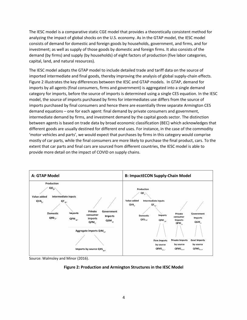
Figure 4: Percentage Changes in Exports of Intermediate Inputs and Final Goods of a Region Due to

Closures in that Region (Direct) and in Other Regions (Indirect)

The large decline in U.S. exports from the indirect effects is also due to the importance of the ROW to

U.S. exports. Both China and the U.S. export more essential goods to the ROW as a result of the ROW’s

mandatory closures, but China is also able to export more non-essential goods, while the USA does not.

The reason for this is primarily that China exports a higher share of final goods than the USA, which

exports primarily intermediates. With non-essential businesses in the ROW closed, demand for final

non-essential goods rises, while demand for intermediates falls. China’s exports to the ROW rise, while

USA exports fall. We are able to capture this difference between Chinese and US exports because we

are using a CGE model supplemented with supply-chain data.

VI. Sectoral Impacts

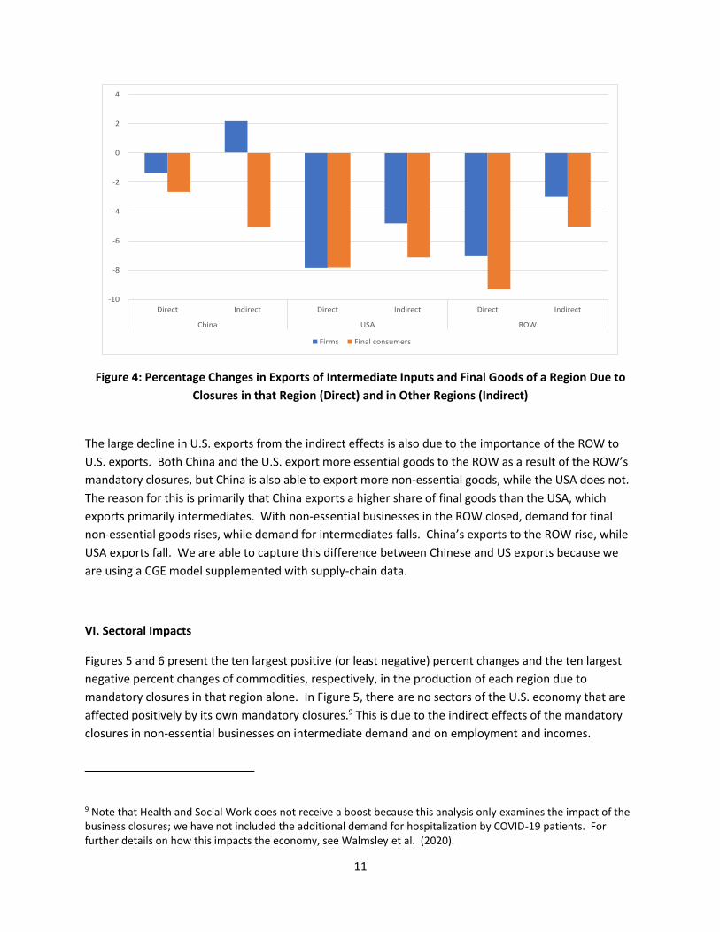
Figures 5 and 6 present the ten largest positive (or least negative) percent changes and the ten largest

negative percent changes of commodities, respectively, in the production of each region due to

mandatory closures in that region alone. In Figure 5, there are no sectors of the U.S. economy that are

affected positively by its own mandatory closures.9 This is due to the indirect effects of the mandatory

closures in non-essential businesses on intermediate demand and on employment and incomes.

9 Note that Health and Social Work does not receive a boost because this analysis only examines the impact of the business closures; we have not included the additional demand for hospitalization by COVID-19 patients. For further details on how this impacts the economy, see Walmsley et al. (2020).

-10

-8

-6

-4

-2

0

2

4

Direct Indirect Direct Indirect Direct Indirect

China USA ROW

Firms Final consumers

12

Figure 5. Ten Largest Positive (or Least Negative) % Changes in Production Due to Mandatory Closures

in that Region Alone

13

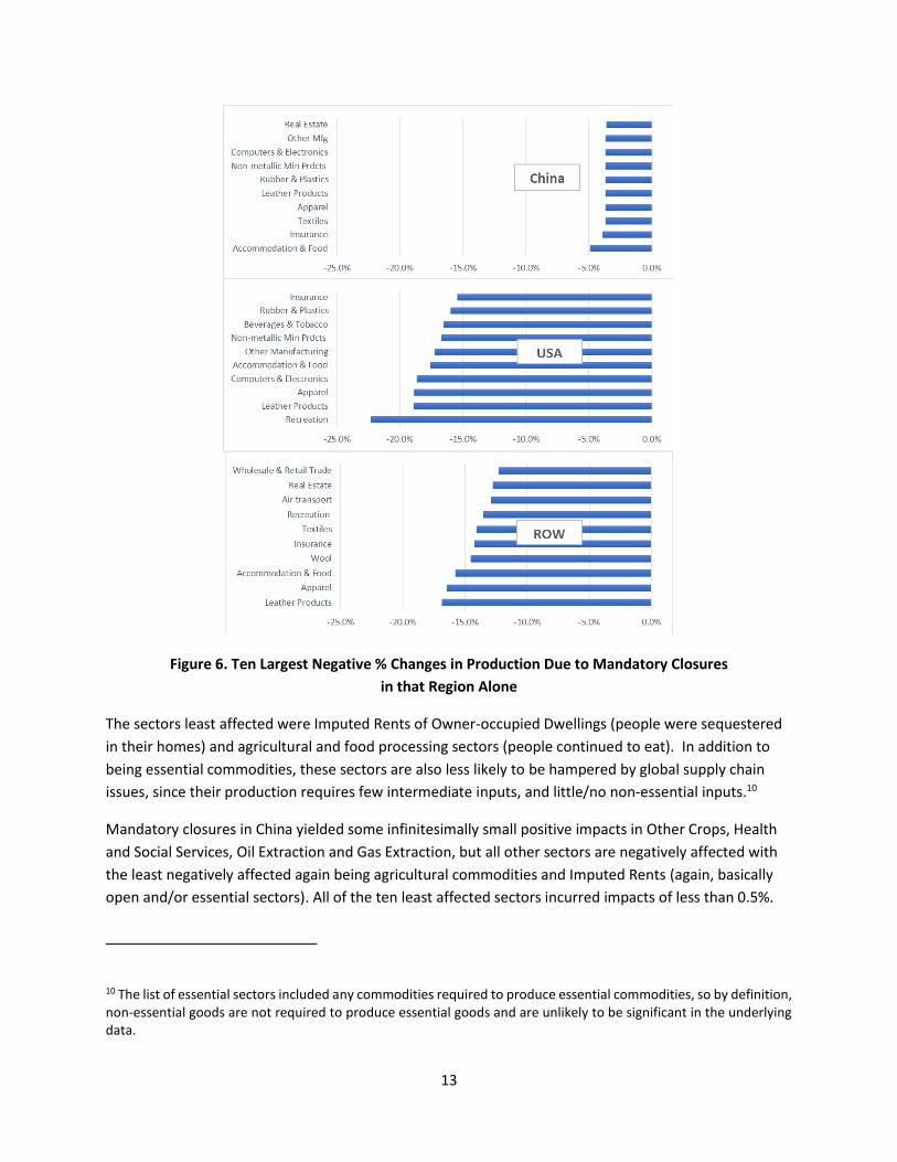
Figure 6. Ten Largest Negative % Changes in Production Due to Mandatory Closures

in that Region Alone

The sectors least affected were Imputed Rents of Owner-occupied Dwellings (people were sequestered

in their homes) and agricultural and food processing sectors (people continued to eat). In addition to

being essential commodities, these sectors are also less likely to be hampered by global supply chain

issues, since their production requires few intermediate inputs, and little/no non-essential inputs.10

Mandatory closures in China yielded some infinitesimally small positive impacts in Other Crops, Health

and Social Services, Oil Extraction and Gas Extraction, but all other sectors are negatively affected with

the least negatively affected again being agricultural commodities and Imputed Rents (again, basically

open and/or essential sectors). All of the ten least affected sectors incurred impacts of less than 0.5%.

10 The list of essential sectors included any commodities required to produce essential commodities, so by definition, non-essential goods are not required to produce essential goods and are unlikely to be significant in the underlying data.

14

For the ROW, only the Imputed Rents sector is positively affected. Health and Social Services is slightly

negatively affected, but the remaining least affected sectors all exceed impacts of 1.4% or more, in

absolute terms. All of the most negatively impacted sectors among those least affected are agricultural

or food processing, except for Public Administration and Defense.

Figure 6 presents the results for the most negatively affected sectors, typically nonessential (see

Appendix for further details on nonessential sector closures). In the case of the U.S., the most adversely

impacted sectors due to its own closures are Recreation, Food & Accommodation-related products and

various manufactured commodities. The Recreation sector losses are more than 20% and several

manufacturing sector declines are nearly as high. For China, the top two sectors are Accommodation &

Food and Insurance. The next seven most-affected sectors are in manufacturing, while the tenth is Real

Estate.11 These results reflect lower consumer expenditures. The losses in the ten most negatively

affected sectors in ROW all exceed 12%. The majority are consumer goods/services sectors of various

kinds that are either directly impacted by the mandatory closures, or indirectly impacted by the closure

of other sectors or both.

Figures 7 and 8 present the ten largest positive (or least negative) percent changes and ten largest

negative percent changes in U.S. production due to mandatory closures in each region alone,

respectively. For the U.S., the results in Figure 7 are the same as in Figure 5 -- again, the smallest

reduction in sectoral output is in Imputed Rents and Health & Social Work, followed by eight agricultural

and food processing sectors. However, for China’s closures, the U.S. economy receives a boost in its

sectoral output of manufacturing sectors with which it competes with China in terms of import

substitution (see the China column). The boost is primarily due to an increase in domestic demand as

consumers, unable to purchase Chinese goods, substitute towards domestically produced goods. U.S.

exports shown in Table 2 also decline, as less goods are exported to both China and to a lesser extent

the rest of the world. The U.S. gains in only one commodity from the Rest of the World closures, and

many sectors are affected only minimally. The total commodity hit on the U.S. economy shown in the

last section of Figure 7 is dominated by its own-effects.

Figure 8 shows largest negatively affected sectors in the U.S. due to its own and other regions’ closures

and are again the same results for the “U.S. Only” case as shown in the counterpart section in Figure 6 --

the Recreation sector is estimated to experience losses of more than 20% on an annualized basis and

the declines in several manufacturing sectors are nearly as high. The U.S. is relatively insulated on a

commodity-by-commodity basis from closures in China, with only one sector impacted positively, and

even then at only slightly more than 1%. However, the U.S. is significantly impacted by ROW, mainly in

terms of energy extraction/processing and manufacturing sectors.

11 The percentage of overall output reduction in China due to closures was 3.71%. Sectoral Changes that deviated from this amount occurred because of general equilibrium effects in an economy.

15

Figure 7. Ten Largest Positive % (or Least Negative) Changes in U.S. Production due to Mandatory

Closures in Each Region

16

Figure 8. Ten Largest Negative % Changes in U.S. Production Due to Mandatory Closures

in Each Region

VI. Summary and Conclusion

Overall, international trade linkages have significant effects on the regional and global impacts of

COVID-19. Trade acts to spread primarily negative impacts across countries/regions through demand

17

and supply for final goods and services and through supply-chain effects relating to intermediate goods.

At the same time, if international trade were shut down or restricted in the face of the pandemic, the

negative impacts could be much worse for some countries/regions for lack of adequate domestic

production and the exacerbation of supply-chain bottlenecks. Overall, the effects of trade linkages

depend on a country’s/region’s relative self-sufficiency, role in the global supply-chain, reliance on

primary commodity production, and stringency and length of market closures. Many of these effects

differ for individual commodities as well, depending on whether or not they are deemed “essential”, or

whether or not they are primary commodities, or the extent to which their production requires non-

essential intermediate inputs.

Many of the results in this paper follow intuition. We find that the U.S. economy is relatively more

insulated from the spatial transmission of economic impacts of COVID-19 than are the other two

regions. We find that the impacts on China are relatively small, owing primarily to the short duration of

its closures, which enable it to gain a temporary trading edge on the U.S. and ROW. We also find that

sectors least affected are those that were deemed essential or otherwise able to remain open in all

three regions. At the same time, the analysis uncovered some anomalies. For example, China reaps a net

indirect export gain due to closures in other regions. In addition, several U.S. manufacturing sectors reap

gains because of the closures in China.

We acknowledge some limitations of our analysis. First, we have used a computable general equilibrium

modeling approach, which typically is best suited for long-run analyses in which the economy can be

thought of returning to equilibrium after it is shocked. However, the analysis does seem to have

provided reasonable results for the impacts of short-run shocks. Still the level effects should be viewed

as lower bounds, because they smooth out bottlenecks and other disequilibria, though, at the same

time, we note that we have presented the analysis in terms of percentage effects, which are less

susceptible to the aforementioned limitation. At the same time, we note that we have not included

offsetting effects of subsequent pent-up demand stemming from the build-up of savings associated with

the inability to venture out to shop or because of the unavailability goods being produced.

Second, our results also rely on the estimated elasticities taken from the literature and used in the GTAP

database and our assumptions about real consumption of essentials. Our assumptions regarding real

consumption of essentials ensures that consumers continue to purchase and firms continue to produce

essential items, despite declining incomes and the closure of non-essential businesses, although our

sensitivity tests indicate that it has only a small impact on the macroeconomic impacts in the U.S.

Finally, the aggregation of the rest of the world into one category limits the ability to fully capture the

supply-chain effects that are likely to have occurred in that region (though it is unlikely to have any

significant impact on the U.S. results).

One concern that has been raised is that the vulnerabilities to global supply-chain spreading of negative

impacts will strengthen anti-globalization sentiment. This could manifest itself in trade restrictions and

business decisions to reduce global interactions. However, more reasonable remedies without the

deleterious effects on economic efficiency would be to identify other ways to decrease vulnerability,

such as lining up alternative suppliers, increasing stockpiles of critical materials, and resource pooling, all

forms of economic resilience (Rose, 2017; Wei et al., 2020). Such policies apply to more specific

concerns as well. For example, countries cannot rely on international trade to make up deficiencies in

18

personal protective equipment (PPE) and other essential goods and services in the presence of a truly

global pandemic. In addition to the aforementioned resilience tactics, countries can further reduce their

vulnerability through flexible production processes domestically to be able to shift to goods in short

supply.

We also offer the following suggestions for future research. First would be to increase the resolution of

the analysis by distinguishing among various sub-categories of rest of world countries. Second would be

to improve the linkages between COVID infections, hospitalizations, the demand for health care in

general, and for inputs into those services. Third would be to improve the tracking of savings due to

consumer spending limitations and the subsequent extent and timing of pent-up demand. Related to

this would be to track people’s avoidance behavior even after mandatory closure orders are lifted due

to lingering fears, including the influence on people’s consumption behavior during the recovery from

the pandemic (e.g., increased online shopping instead of in-store shopping, reduced air travel and

tourism industry demand).

Funding: This paper is based upon work supported by the U.S. Department of Homeland Security under

Grant Award Number 17STQAC00001-03-00; and by the Centers for Disease Control and Prevention

under contract number 75D30120P08155. The views and conclusions contained in this document are

those of the authors and should not be interpreted as necessarily representing the official policies,

either expressed or implied, of its sponsors. The authors are responsible for any remaining errors or

omissions.

Acknowledgements: The authors wish to thank Konstantinos Papaefthymiou for his research assistance.

Declaration of interest statement: The authors declared no potential conflicts of interest with respect

to the research, authorship and/or publication of this article.

19

References

Aloui, D., S. Goutte, K. Guesmi, and R. Hchaichi. 2020. “COVID 19’s Impact on Crude Oil and Natural Gas

S&P GS Indexes,” SSRN 3587740. http://dx.doi.org/10.2139/ssrn.3587740

Baldwin, R. and B. di Mauro. 2020. “Introduction,” in R. Baldwin and B. di Mauro, Economics in the Time

of COVID-19. Centre for Economic Policy Research. CEPR Press, London UK.

Baldwin, R. and E. Tomiura. 2020. Thinking ahead about the trade impact of COVID-19,” in R. Baldwin

and B. di Mauro, Economics in the Time of COVID-19. Centre for Economic Policy Research. CEPR Press,

London UK.

Brockmeier, M., 2001. “A Graphical Exposition of the GTAP Model”, GTAP Technical paper #08, Center

for Global Trade Analysis, Lafayette: IN. available at:

https://www.gtap.agecon.purdue.edu/resources/res_display.asp?RecordID=311

Corong, E., T. W. Hertel, R. McDougall, M. E. Tsigas, and D. van der Mensbrugghe. 2017. “The Standard

GTAP Model, Version 7,” Journal for Global Economic Analysis 2(1): 1-119.

Gharib, C., S. Mefteh-Wali, and S. Ben Jabeur. 2021. “The bubble contagion effect of COVID-19 outbreak:

Evidence from crude oil and gold markets,” Finance Research Letters 38: 101703.

Guan et al. 2020. “Global supply-chain effects of COVID-19 control measures,” Nature Human Behaviour

4: 577 – 587.

Hertel, T. W. and M. E. Tsigas. 1997. “Structure of GTAP,” in T.W. Hertel (ed.), Global Trade Analysis:

Modeling and Applications, New York: Cambridge, pp. 13-73.

Horridge, M., M. Jerie, D. Mustakinov and F. Schiffmann (2018), GEMPACK manual, GEMPACK Software,

ISBN 978-1-921654-34-3

Jiang, P., Y. Fan, and J. Klemes. 2021. “Impacts of COVID-19 on energy demand and consumption:

Challenges, lessons and emerging opportunities,” Applied Energy 285(1): 116441.

Meinen, P., R. Serafini, and O. Papagalli. 2021. “Regional Economic Impact of COVID-19: The Role of

Sectoral Structure and Trade Linkages,” ECB Working Paper No. 2021/2528.

https://papers.ssrn.com/sol3/papers.cfm?abstract_id=3797148

Rose, A. 2017. “Benefit-Cost Analysis of Economic Resilience Actions,” in S. Cutter (ed.) Oxford Research

Encyclopedia of Natural Hazard Science, New York: Oxford.

Statista. 2020. Change in remote work trends due to COVID-19 in the United States in 2020.

https://www.statista.com/statistics/1122987/change-in-remote-work-trends-after-covid-in-usa/

U.S. Bureau of Economic Analysis (BEA). 2020. GDP by State. https://www.bea.gov/data/gdp/gdp-state.

U.S. Bureau of Labor Statistics. 2019. “Table 1. Workers who could work at home, did work at home, and

were paid for work at home, by selected characteristics, averages for the period 2017-2018.”

https://www.bls.gov/news.release/flex2.t01.htm

20

U.S. Bureau of Labor Statistics. 2020a. Supplemental Data Measuring the Effects of the Coronavirus

(COVID-19) Pandemic on the Labor Market. https://www.bls.gov/cps/effects-of-the-coronavirus-covid-

19-pandemic.htmU.S. Bureau of Labor Statistics. 2020b. Labor Productivity and Costs.

https://www.dol.gov/newsroom/economicdata/prod_08142020.pdf

Verschuur, J., E. Koks, and J. Hall. 2021. “Observed impacts of the COVID-19 pandemic on global trade,”

Nature Human Behaviour 5: 305-307.

Walmsley T. L., and P. Minor. 2016. “ImpactECON Global Supply Chain Model: Documentation of Model

Changes,” Working Paper No. 06, ImpactECON, Boulder, CO. https://impactecon.com/resources/supply-

chain-model/

Walmsley T. L., and P. Minor. 2020. “U.S. Trade Actions Against China: A Supply Chain Perspective,”

Foreign Trade Review 55(3): 337-371.

Walmsley, T., A. Rose and D. Wei. 2020. “Impact on the U.S. Macroeconomy of Mandatory Business

Closures in Response to the COVID-19 Pandemic,” Applied Economics Letters.

Walmsley, T., A. Rose and D. Wei. 2021. “The Impacts of the Coronavirus on the Economy of the United

States,” Economics of Disasters and Climate Change 5(1): 1-52.

Wei, D., Z. Chen and A. Rose. 2020. “Evaluating the Role of Resilience in Recovering from Major Port

Disruptions: A Multi-Regional Analysis,” Papers in Regional Science 99(6): 1691-1722.

Wikipedia. 2020. “COVID-19 pandemic lockdowns,” https://en.wikipedia.org/wiki/COVID-

19_pandemic_lockdowns

21

Appendix A. Mandatory Closures and Reopening Data for the U.S.

Appendix Table A1. Stay-at-Home Orders and Mandatory Closures by U.S. State (March to June 2020)

State Order declared

Order expired or reopening started

Length (days) of Closure

Note

Alabama 3-Apr 30-Apr 27 Alaska 28-Mar 24-Apr 27 Arizona 30-Mar 15-May 46

Arkansas

Did not have a statewide stay-at-home order, but some business restrictions lifted starting May 6

California 19-Mar 12-May 54 Starting May 12, restaurants and shopping centers can open in counties that meet certain criteria

Colorado 26-Mar 26-Apr 31 Connecticut 23-Mar 20-May 58 DC 1-Apr 8-Jun 68 Delaware 24-Mar 31-May 68 Florida 3-Apr 4-May 31 Georgia 3-Apr 30-Apr 27

Hawaii 25-Mar 7-May 43 Order set to expire May 31 but reopening started May 7

Idaho 25-Mar 30-Apr 36 Illinois 21-Mar 31-May 71 Indiana 25-Mar 4-May 40

Iowa

Did not have a statewide stay-at-home order, but loosened restrictions in most counties starting May 1

Kansas 30-Mar 3-May 34 Kentucky 26-Mar 20-May 55 Louisiana 22-Mar 15-May 54

Maine 2-Apr 11-May 39 Stores (May 11) and restaurants (May 18) will be allowed to reopen in certain rural counties

Maryland 30-Mar 15-May 46 Massachusetts 24-Mar 18-May 55 Michigan 24-Mar 28-May 65 Minnesota 27-Mar 17-May 51 Mississippi 3-Apr 27-Apr 24 Missouri 6-Apr 3-May 27 Montana 26-Mar 26-Apr 31

Nebraska

Did not have a statewide stay-at-home order, but some business restrictions lifted starting May 4

Nevada 1-Apr 9-May 38 New Hampshire 27-Mar 11-May 45

Order set to expire May 31 but reopening started May 11

New Jersey 21-Mar 5-Jun 76

22

New Mexico 24-Mar 16-May 53 Retailers, offices and houses of worship can open at limited capacities beginning May 16

New York 22-Mar 15-May 54 Limited reopening in five regions starting May 15

North Carolina 30-Mar 8-May 39 Order set to expire May 31 but reopening started May 8

North Dakota

Did not have a statewide stay-at-home order, but some business restrictions lifted starting May 1

Ohio 23-Mar 15-May 53 Order set to expire May 29 but reopening started May 15

Oklahoma

Did not have a statewide stay-at-home order, but some business restrictions lifted starting April 24

Oregon 23-Mar 15-May 53 Retail stores statewide to reopen on May 15

Pennsylvania 1-Apr 8-May 37 Counties to open in phases

Rhode Island 28-Mar 8-May 41

South Carolina 7-Apr 4-May 27 The reopening began with retail stores around April 20

South Dakota

Did not have a statewide stay-at-home order, but state announced a "Back to Normal" plan on April 28

Tennessee 1-Apr 30-Apr 29 Texas 2-Apr 30-Apr 28

Utah

Did not have a statewide stay-at-home order, but some business restrictions lifted starting May 1

Vermont 24-Mar 15-May 52 Virginia 30-Mar 15-May 46 First phase of reopening starting May 15

Washington 25-Mar 11-May 47 Small counties were approved for partial reopenings

West Virginia 23-Mar 3-May 41 Wisconsin 24-Mar 13-May 50

Wyoming

Did not have a statewide stay-at-home order, but some business restrictions lifted starting May 1

Appendix Table A2. Percentage Reduction of Output by Sector in the U.S. Due to Mandatory Closures

and Phased-in Reopening (January to July 2020)

(with Telecommuting)

# Sector Mandatory

Closure Categorya

% Reduction in U.S. annual GDP

Notes for Mandatory Closures Mandatory

Closures Reopening

1 Rice 3 0.0% 0.0%

2 Wheat 3 0.0% 0.0%

3 Other Grains 3 0.0% 0.0%

4 Veg & Fruit 3 0.0% 0.0%

5 Oil Seeds 3 0.0% 0.0%

6 Cane & Beet 3 0.0% 0.0%

7 Fibers crops 3 0.0% 0.0%

8 Other Crops 3 0.0% 0.0%

9 Cattle 3 0.0% 0.0%

23

10 Other Animal Products 3 0.0% 0.0%

11 Raw milk 3 0.0% 0.0%

12 Wool 3 0.0% 0.0%

13 Forestry 3 0.0% 0.0%

14 Fishing, hunting, trapping, etc. 3 0.0% 0.0%

15 Coal: mining 3 0.0% 0.0%

16 Oil: extraction of crude petroleum 3 0.0% 0.0%

17 Gas: extraction of natural gas 3 0.0% 0.0%

18 Other Mining Extraction 3 0.0% 0.0%

19 Cattle Meat 3 0.0% 0.0%

20 Other Meat 3 0.0% 0.0%

21 Vegetable Oils 3 0.0% 0.0%

22 Milk: dairy products 3 0.0% 0.0%

23 Processed Rice: semi- or wholly milled 3 0.0% 0.0%

24 Sugar and molasses 3 0.0% 0.0%

25 Other Food 3 0.0% 0.0%

26 Beverages and Tobacco products 2 2.9% 1.0% Closure: Tobacco products

27 Manufacture of textiles 1 10.6% 4.3%

28 Manufacture of wearing apparel 1 14.1% 4.2%

29 Manufacture of leather and related products

1 14.1% 4.2%

30 Lumber 3 0.0% 0.0%

31 Paper and Paper Products 3 0.0% 0.0%

32 Petroleum and Coke Products 3 0.0% 0.0%

33 Manufacture of chemicals and products

3 0.0% 0.0%

34 Manufacture of pharmaceuticals, medicinal chemical and botanical products

3 0.0% 0.0%

35 Manufacture of rubber and plastic products

1 11.5% 4.1%

36 Manufacture of other non-metallic mineral products

1 12.0% 4.1%

37 Iron & Steel: basic production and casting

3 0.0% 0.0%

38 Non-Ferrous Metals: production and casting of copper, aluminum, zinc, lead, gold, and silver

3 0.0% 0.0%

39 Manufacture of fabricated metal products, except machinery and equipment

3 0.0% 0.0%

40 Manufacture of computer, electronic and optical products

1 13.8% 4.3%

41 Manufacture of electrical equipment 3 0.0% 0.0%

42 Manufacture of machinery and equipment n.e.c.

3 0.0% 0.0%

43 Manufacture of motor vehicles, trailers and semi-trailers

3 0.0% 0.0%

44 Manufacture of other transport equipment

3 0.0% 0.0%

24

45 Other Manufacturing: includes furniture

1 12.7% 4.2%

46 Electricity; steam and air conditioning 3 0.0% 0.0%

47 Gas manufacture, distribution 3 0.0% 0.0%

48 Water supply; sewerage, waste management and remediation activities

3 0.0% 0.0%

49 Construction 2 2.9% 1.3% Closure: all construction except for emergency repair or maintenance

50 Wholesale and retail trade; repair of motor vehicles and motorcycles

2 5.4% 1.9% Closure: Retail except for Grocery Stores, Special Food Stores, Gas Stations, etc.

51 Accommodation, Food and service activities

2 9.3% 4.2% Open: Accommodation; Closure: Food services except for take out

52 Land transport and transport via pipelines

2 2.2% 0.9%

Transportation sectors are essential sectors. However, there have been service reductions / route eliminations caused by a combination of reduced economic activities due to shutdowns, drops in demand, reduced number of transit workers available to work, and the need to implement safety precautions. Based on data from various sources, we estimated that the Air Transportation, Rail Transportation, Water Transportation, and Transit Transportation experienced reduction in service by 66%, 47.5%, 50%, and 50%, respectively during the mandatory closure period.

53 Water transport 2 4.7% 2.1%

54 Air transport 2 8.3% 3.7%

55 Warehousing and support activities 3 0.0% 0.0%

56 Information and communication 2 0.5% 0.4% Closure: Motion Picture and Video Industries, Sound Recording Industries, etc.

57 Other Financial Intermediation: auxiliary activities but not insurance and pensions

2 1.4% 1.1% Closure: Securities, Commodity Contracts, and Other Financial Investments and Related

58 Insurance 3 0.0% 0.0%

59 Real estate activities 1 7.6% 6.2%

60 Other Business Services not elsewhere classified

2 5.1% 4.1% Closure: All except for Scientific Research & Development Services, Waste Management, and some Administration & Support Services

61 Recreation & Other Services 1 10.4% 12.0%

62 Other Services (Government) 2 3.6% 1.5% Closure: All except for emergency services

63 Education 1 4.1% 6.7%

64 Human health and social work 3 0.0% 0.0% Mostly open; exception: Civic and Social Organizations

65 Dwellings: imputed rents of owner-occupied dwellings

3 0.0% 0.0%

a Mandatory Closure Categories:

1. Sector is entirely non-essential and thus is completely shut down

2. Sector for which only some subsectors are non-essential (see notes in the last column)

3. Sector that is essential and thus still able to operate in its usual manner to the extent possible. (Telecommuting adjustment is

based on data presented in Table A2).