Spatial Patterns of Fertility Transition in Indian Districts · ment.4 A few studies have also...

POPULATION AND DEVELOPMENT REVIEW 27(4) :713–738 (DECEMBER 2001) 713

Spatial Patterns ofFertility Transitionin Indian Districts

CHRISTOPHE Z. GUILMOTO

S. IRUDAYA RAJAN

OVER THE PAST five decades, numerous studies have assessed levels, trends,differentials, and determinants of fertility in India. The conclusion is thatfertility decline has been low to moderate except for a few pockets of morerapid transition. Until recently, the analysis of demographic transformationin India has been limited to fertility indicators at the state level. The dis-trict-level data from the censuses of 1981 and 1991 portrayed a much morecomplex situation in the country as fertility differentials often proved to beas substantial within states as between states. (Figure 1 displays Indian statesand large cities.) Because of India’s cultural, economic, and geographicaldiversity, the magnitude of regional variations in fertility levels is much largerthan that in China, and comparison with the demographic history of Eu-rope or of the former Soviet Union would be more appropriate.1

Within the context of demographic heterogeneity, this article seeks toupdate our knowledge on fertility levels in India and to extend our under-standing of the mechanisms behind regional variations. We present the re-sults of a new estimation procedure to reconstruct the Indian fertility tran-sition and describe some of its spatial and statistical properties. Rather thantest hypotheses on fertility–economy–society linkages through an econo-metric model,2 we focus on the spatial structuring of reproductive behaviorin India: fertility is examined as a regionalized variable, that is, a variablewhich is assumed to be spatially continuous.3 As our maps suggest and thegeostatistical analysis demonstrates, spatial variations of fertility in India arefar from random, a fact that has potentially significant implications for ourinterpretation of fertility decline. Specifically, we suggest that preoccupa-tion with the effect on fertility of factors that are poorly correlated withspatial location, such as family planning campaigns or structural transfor-mations of the economy, may have concealed the progression of fertilitychange through diffusion processes at the microlevel.

714 S P A T I A L P A T T E R N S O F F E R T I L I T Y T R A N S I T I O N I N I N D I A N D I S T R I C T S

FIGURE 1 Indian states and major cities

LAKSHADWEEP

ANDAMAN and NICOBAR islands

TAMILNADU

KERALA

KARNATAKA ANDHRAPRADESH

MAHARASHTRA

ORISSA

BIHAR

ASSAM

ARUNACHAL

PRADESH

WESTBENGALMADHYA PRADESH

GUJARAT

PUNJAB

JAMMU andKASHMIR

HIMACHALPRADESH

RAJASTHAN

HARY

ANA

UTTAR PRADESH

MEGHALAYA

MANIPUR

NAGALAND

MIZORAMTRIPURA

SIKKIM

PONDICHERRY

GOA

•

BANGALORE • • CHENNAI

• PUNE

• KANPUR

•

•

MUMBAI •

AHMEDABAD

BOPAL

HYDERABAD

CHANDIGARH

DELHI

• KOLKATA

Sources for studying the Indian fertility transition

Using the age distribution of the 1961 and 1971 Indian censuses, Adlakhaand Kirk (1974) concluded that the level of fertility during the early 1960sdid not differ substantially from the level during the early 1950s. As theysummarized their findings: “The crude birth rate in India declined by be-tween seven and 10 per cent, from a level of about 45 in 1951–61 to about40.5–42.0 in 1961–71” (p. 400). Extending the same data up to the 1981census, Rele (1987) concluded that the total fertility rate remained stable ataround 6 during the 1950s and into the first half of 1960s. The turning

C H R I S T O P H E Z . G U I L M O T O / S . I R U D A Y A R A J A N 715

point in Indian fertility seems to have occurred around 1966, with an esti-mated TFR of 5.8 in 1966–71, 5.3 in 1971–76, and 4.7 in 1976–81. Theestimated levels and trends of fertility for 14 major Indian states showedremarkable geographic consistency, with northern states having higher fer-tility than southern states in 1961–66 and, with only slight modifications,in 1976–81.

Jain and Adlakha (1982) corroborated that the fertility rate in Indiabefore 1961 was high and stable. Their analysis indicated that the crudebirth rate in India fell from 41 births per thousand in 1972 to 35–37 in1978 and that the decline was primarily caused by declining age-specificfertility rates. As in the case of two national surveys, analysis of the agedistributions of the censuses of 1971 and 1981 suggested that a major fertil-ity decline was underway during the intercensal period (Preston and Bhat1984). A large share of this decline probably occurred in the late 1970s; thefertility reduction seems to have been slightly faster in the southern states.

Assessing the degree of heterogeneity in fertility behavior within In-dian states, Guilmoto (2000) concluded that fertility decline began in theperiphery along the coasts and in the extreme south, and spread progres-sively to encircle the region around the Ganges Valley, the heart of tradi-tional India, where fertility has scarcely declined. The Hindi-speaking coreregion is characterized by high fertility, an entrenched patriarchal value sys-tem, economic underdevelopment, predominance of Brahminical influence,and exclusion of women from education. In south India, Kerala has longbeen recognized for its rapid fertility transition, occurring in the absence ofsignificant economic development as conventionally measured. Female lit-eracy is the single most frequently cited indicator in explaining this achieve-ment.4 A few studies have also focused on the recent fertility experience ofTamil Nadu and of south India in general.5 Tamil Nadu is notable for hav-ing achieved replacement-level fertility without reaching Kerala’s high levelof female literacy or its low level of infant mortality. Using the state-levelindicators of fertility, a number of researchers have grouped Indian statesinto two demographic regimes: south with low fertility and north with highfertility.6

Very few studies permit assessment of fertility levels and trends at thedistrict level. For the first time in the 1981 census, the Registrar General ofIndia provided district-level estimates of fertility and mortality using indi-rect techniques (Registrar General of India 1988, 1989), and a few studiesusing these data have appeared since then.7 For the 1991 census, the Regis-trar General’s indirect estimates of fertility and mortality at the district levelas well as a few estimates by individual researchers are now available.8 Bhat(1996), using the reverse-survival method, produced birth rates at the dis-trict level for the periods 1974–80 and 1984–90 and also analyzed cross-sectional variations in fertility.


More recently, using data generated by the National Family HealthSurvey (NFHS), Bhat and Zavier (1999) analyzed the differentials in fertil-ity within 76 regions of the country. Among the 76 regions around 1975,none had a total fertility rate under 3 births, 12 regions were in the rangeof 3–4, 35 in the range of 4–5, and the remaining 29 regions were above 5.In 1987, ten regions had total fertility rates under 3, 34 were in the rangeof 3–4, 24 in the range of 4–5, and only eight regions were above 5. Ineffect, after a lapse of 12–13 years, only 30 percent of the regions had re-mained in their previous total fertility class. The NFHS estimates confirmthe earlier finding (Bhat 1996) of substantial reductions in fertility through-out the country, not just in a few pockets.

Although the Sample Registration Survey (SRS) has been widely usedto study fertility since the 1970s, it provides estimates of fertility for majorstates only. In recent years the SRS has published estimates for smaller statesand union territories but does not provide information on fertility at thedistrict level. Surveys conducted in a number of states (Mysore PopulationStudy, for Karnataka; Gandhigram Institute Survey, for Tamil Nadu; KeralaFertility Survey, for Kerala, to name a few) focus on fertility and its deter-minants at the state level. Against this background, this article aims to pro-vide a new set of fertility estimates at the district level starting from the1950s. We use a new database that integrates all district-level age data drawnfrom the 1961, 1971, 1981, and 1991 censuses. We devise a new indexbased on child–woman ratios computed from census age distributions.9

From the child–woman ratio to thechild–woman index

Estimates derived from child–woman ratios (CWRs)10 can be used to recon-stitute fertility trends at the district level over a 40-year period. The combi-nation of two CWRs calculated by using different numerators and denomi-nators in the ratio enables us to estimate fertility levels for each five-yearinterval. Specifically, we calculated CWRs as children aged 0–4 divided bywomen aged 15–49 and as children aged 5–9 divided by women aged 20–54. For example, 1961 CWR values yield estimates for 1951–55 (using the5–9-year age group as numerator) and for 1956–60 (using the 0–4-year agegroup). Our 1961–91 database thus provides a set of district-level fertilitymeasurements for eight five-year intervals from 1951–56 to 1986–91.

Compared with other fertility indexes, the child–woman ratio has sev-eral limitations. The main shortcoming is that this ratio is based on surviv-ing children in different age groups and not on the number of live births.The following simplified formula highlights this flaw:

CWR = children/women =(births x child survival) / (women x adult survival).


Mortality differentials between regions or census periods may cause varia-tions in CWRs and make comparisons between CWRs potentially mislead-ing. Raw values of the CWR reflect fertility levels as well as child mortalitylevels. Furthermore, because India was characterized by rapid mortality de-cline during the period in question, inter-temporal variations in CWRs im-perfectly reflect fertility changes over time. Correcting for the mortality fac-tor is therefore a first requirement in improving the index.

A second limitation relates to the simultaneous use of two differentCWRs that are not directly comparable because they are based on differentage groups. As noted above, we use both the 0–4 and the 5–9-year agegroups to reconstruct fertility during the two quinquennia preceding thecensus year: the two CWRs require adjustment to be comparable.

Apart from the effects of child and adult mortality just noted, otherlimitations to the use of the CWR are related to the changing shape of theage distributions of women 15–54; gains and losses through net in- or out-migration; and the accuracy of age enumeration and age reporting. No fullyadequate correction is feasible for the distortions these factors cause in theCWRs as an index of fertility. It is worth stressing, however, that our at-tempt is not to estimate fertility values per se, but to arrive at a comparativeindex of fertility trends over time and of differentials by region. Hence, wehave not attempted a correction for mortality variations among the adultfemale population, nor have we tried to take into account migration. Weconsider these factors minor in explaining CWR differentials compared tothe effect of the fertility component as reflected in the census data for chil-dren aged 0–9. We have also used the raw total of the adult female popula-tion aged 15–49 and 20–54 as a denominator for calculating CWRs insteadof weighting age groups by their respective share according to an estimatedperiod fertility schedule.11 For lack of reliable and detailed estimates, wehave also ignored the possible impact of changes in the completeness of thecensus and in the accuracy of age reporting. In view of the poorer quality ofregistration and age reporting in the earlier censuses, such changes may beresponsible for the erratic age distributions observed in some districts. Thestandardization procedure explained below, which yields a measure we callthe child–woman index or CWI, seeks to minimize the effect of these prob-lems in the underlying statistics.12

Details of the computation of the new CWI are given in the Appendix.The index provides a comparative fertility indicator at the district level forthe eight five-year periods starting with 1951–55 and ending with 1986–90. As a feature of the standardization, we equate the average value of theCWI over 1961–91 to one.

To illustrate the effect of our correction and standardization procedures,Figure 2 presents the all-India values derived from child–woman ratios, start-ing with the original CWR

values computed from the raw census age distri-

butions. Once corrected for mortality, the ratio displays more pronounced


variations because the impact of declining mortality over four decades isremoved. However, the serrated profile of these lower two curves showsthat the CWR based on children aged 5–9 and women aged 20–54 is notdirectly comparable to the CWR based on children aged 0–4 and womenaged 15–49. In fact, the former ratio (used for the 1951–56, 1961–66, 1971–76, and 1981–86 quinquennia) seems to overestimate fertility when com-pared to the latter ratio (used for the other quinquennia). After standard-ization and limited smoothing (see Appendix), the final child–woman indexprovides a reliable indicator of fertility variations across periods and districts.

A statistical description of the results (see Table 1) shows that whileaverage fertility levels decreased after 1961, the variability of fertility indi-

F

F

F

F

F

F

F

F

B

B

B

B

B

B

B

B

I

I

I I

I

I

I I

H H

H

H

H

H

H

H

1951–56 1956–61 1961–66 1966–71 1971–76 1976–81 1981–86 1986–910.5

0.6

0.7

0.8

0.9

1

1.1

1.2

1.3

Ch

ild

–wo

man

rat

io a

nd

ch

ild

–wo

man

in

dex

Period

FIGURE 2 Child–woman ratio and child–woman index, all-India, 1951–91

NOTE: CWRs are computed from census data, using successively children aged 5–9 and children aged 0–4.For description of the correction and standardization procedures, see the Appendix.

Standardized CWR

CWI

CWR correctedfor child mortality

CWR from census

TABLE 1 District averages of the child–woman index, India, 1951–91

1951– 1956– 1961– 1966– 1971– 1976– 1981– 1986–1956 1961 1966 1971 1976 1981 1986 1991

District average 1.155 1.157 1.131 1.076 0.974 0.883 0.825 0.787Standard deviation 0.144 0.137 0.147 0.149 0.136 0.140 0.151 0.166Coefficient of variation(percent) 12.5 11.9 13.1 13.8 14.0 16.0 18.4 21.2

Number of districts usedin the computation 316 316 338 338 331 331 328 328


cators in India almost doubled during the same period. Demographic changein India is now a major differentiating factor among regions that shared acommon profile during the colonial period.

Mapping fertility transition from 1951 to 1991

The next step is to plot the district values on a series of maps covering 40years (1951 to 1991) of demographic transition in India. CWI values arefirst plotted on the map, using the geographical coordinates of district head-quarters. The local fertility values are then converted to a surface map us-ing kriging, a standard geostatistical procedure, to interpolate fertility val-ues on the entire map of India.13 Kriging is the optimal method of spatialinterpolation, and it generates the most accurate estimates of surface val-ues among available methods of spatial smoothing (see Appendix for de-tails on our kriging procedure). The outcome consists of a “grid” made ofsmall square cells (20 km by 20 km). After kriging, local grid values arecontoured using seven value classes. The final result is a set of eight five-year maps depicting fertility transition from 1951 to 1991 (see Figure 3).Because the CWI is corrected and standardized for mortality, comparisonsacross regions and across five-year periods are possible. Although regionalbiases—resulting from such factors as serious age misstatement or differen-tial underenumeration of children—may persist, especially for the 1961 and1971 census data, the mapping enables us to follow regional and all-Indiatrends and to examine 40 years of changes in fertility behavior.

The first two maps in Figure 3, for the 1951–61 period, show the lim-ited variation in pretransitional fertility within India. The northeast, wherethe data quality is admittedly poor, exhibits the highest fertility levels. Sev-eral pockets of moderate fertility are visible both in south India (south Keralaand Tamil Nadu) and in mountainous districts in the western Himalayas.As further maps will show, these areas remain characterized by below-av-erage fertility. An area of moderate fertility comprises several adjacent ru-ral districts in central India across Madhya Pradesh and Maharashtra. Thisfeature disappears in later maps. Although the possible effect of region-spe-cific age misstatement cannot be ruled out, more information is required onpretransitional fertility regimes in India to elucidate this feature.14

Fertility increased across India after 1956 except in the moderate fer-tility areas of south India and the mountainous districts. The rise is espe-cially discernible in western India and in the northern part of the subconti-nent until the 1960s. (This pretransitional rise in fertility is highlighted inDyson and Murphy 1985.)

In the 1960s, fertility decline began in several areas. This reduction ismost pronounced in the southern tip of India.15 The drop in fertility is alsovisible in Tamil Nadu and Kerala, as well as in south Karnataka and Andhra

FIGURE 3 Child–woman index, 1951–91

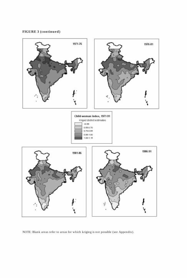
FIGURE 3 (continued)

NOTE: Blank areas refer to areas for which kriging is not possible (see Appendix).


Pradesh. Interestingly, coastal areas both in the west (from Mumbai inMaharashtra to Goa) and in the east (almost the whole of coastal AndhraPradesh) are affected.16 The geographical logic of this decline is pronouncedas all the affected regions are contiguous. Other regions in India exhibitinga downward trend in the fertility index were the high-altitude areas inHimachal Pradesh and Jammu-Kashmir as well as the north of Punjab. Ironi-cally, Punjab, whose wheat-growing plains had reaped the early benefits ofthe Green Revolution during the 1960s, was cited during the same periodas the high-fertility area par excellence in an influential debate on the ra-tionale for fertility behavior in developing countries.17 Adjacent areas in thestate of Haryana and western Uttar Pradesh, where agriculture also madegreat progress during the same period, show no trace of fertility reduction.The Punjab–Haryana border, which more or less demarcates Sikh-dominatedPunjab from Hindu-dominated areas (Haryana and Uttar Pradesh), still sepa-rates areas of low and high fertility, as is evident on our maps for the late1980s.

The first four maps in Figure 3, covering the period 1951–71, showthat the high-fertility areas of northern India gradually formed a single blockcentered near the border between the three states of Rajasthan, UttarPradesh, and Madhya Pradesh. Another core area characterized by high fer-tility comprises the Brahmaputra Valley in the northeast state of Assam,the northern portion of West Bengal, and some smaller states in the north-east such as Meghalaya and Arunachal Pradesh. In other states of the north-east (Nagaland, Manipur, and Mizoram), where many regional tribes have beenChristianized, literacy tends to be higher and fertility is more moderate.

The maps in Figure 3 that pertain to the 1970s, a period characterizedby aggressive family planning campaigns in India, show the gradual spreadof fertility decline across most regions. The fall is most visible in southernIndia, below a line that could be drawn from Gujarat in the west to Cal-cutta in the east. Although the pioneering districts of Kerala and Tamil Naduare still far ahead, fertility decline has been rapid everywhere in south andcentral India. New pockets of pronounced fertility reduction have becomevisible in Gujarat and in southern districts of West Bengal. In the latter re-gion, fertility has already reached a low value in and around the city ofKolkata (formerly Calcutta) by the 1970s, but this downward trend alsomanifests itself in the entire southern part of the state.

The coastal pattern of fertility change is still evident, especially as inte-rior districts in the Deccan Plateau have experienced a less rapid pace ofdemographic change. The eastern tip of Maharashtra (Vidharba) and a fewdistricts in Uttar Pradesh around the cities of Lucknow and Kanpur repre-sent exceptions to early fertility decline in interior India. In the northwest,the fertility decline becomes pronounced in all Punjab districts and in theunion territory of Chandigarh. Fertility decline has still not spread as might


have been expected to adjacent rural areas in Haryana and western UttarPradesh. On the contrary, the decline seems to have expanded fromHimachal Pradesh toward the northwest of Uttar Pradesh (Kumaon), whichcomprises several mountainous districts at the foothills of the Himalayas.

The picture becomes more complex during the 1980s. Although fertil-ity decline is occurring in almost every region of India, persistent differen-tials between subregions give our maps a patchwork appearance. A majorfeature of this period is the significant contraction of the high-fertility zonein India that formerly covered most of Bihar, Madhya Pradesh, Rajasthan,and Uttar Pradesh. Fertility has decreased considerably in central UttarPradesh, while less concentrated decline was underway in Rajasthan andBihar. In the northeast, the demarcation between the western states (Assam,Meghalaya, and Arunachal Pradesh) and the eastern states (Manipur,Mizoram, Nagaland, and Tripura) became more acute, as the latter haverecorded rapid fertility decline. By the late 1980s, fertility in Manipur andNagaland was as low as in south Indian states.

In the south, the fall in fertility rates in the 1980s accelerated nearlyeverywhere. In many districts of Kerala and Tamil Nadu, values of the child–woman index reached a value less than half of those estimated for northIndia. Districts with the lowest values of the index were still highly concen-trated in two pockets, in west Tamil Nadu (Coimbatore region) and in southKerala. Whereas fertility decline in north India has profoundly redrawn themap of fertility differentials, relative variations between subregions in thesouth have been more or less preserved. Only the central region of theDeccan Plateau (central Maharashtra, north Karnataka, and sections of west-ern Andhra Pradesh) seems to have remained a partial exception to fertilitydecline—not unlike the western districts of Uttar Pradesh, where any diffu-sion of the rapid decline in the Punjab and Himachal Pradesh seems to haveremained minimal.

Three fertility profiles

Exploring the individual cases of hundreds of districts that may have littlein common in terms of social, cultural, or economic characteristics wouldbe a tedious exercise. Many local fertility trends may be explained by uniquesets of historical characteristics, bearing little resemblance to conditions inneighboring areas. At the same time, paying attention only to broad re-gional aggregates, such as state average values, would obscure fertility trendsthat stand out on our contour maps. We have, therefore, opted for a statis-tical reexamination of our district-level estimates in order to identify major“fertility profiles” as a means to describe 40 years of demographic change inIndia. Because correction and standardization procedures for the child–woman index yield a consistent time series for several hundred Indian dis-


tricts, we have performed a cluster analysis on this database, using districtsas observation units and the various five-year fertility estimates as variables.The cluster analysis is a technique aimed at providing the best partition ofour district units. After repeated trials, we opted for a three-way partitionof our district sample as the most convenient for analysis and presentation.18

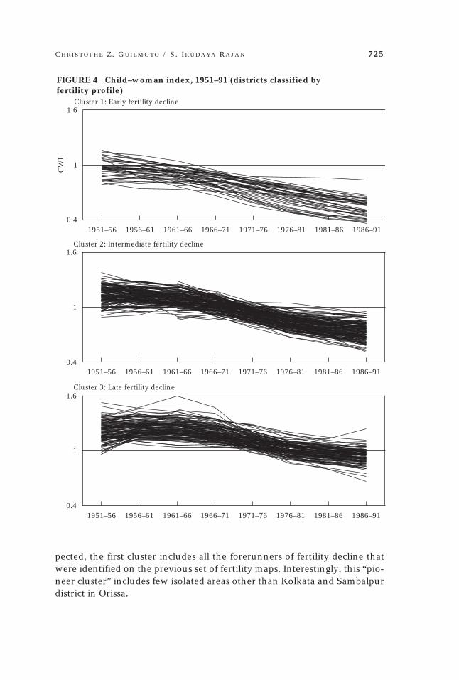
The clusters that divide Indian districts into three fertility groups in-clude respectively 44, 159, and 135 districts. While fertility characteristicsin the three clusters share some structural features such as the downwardtrend over the last 30 years, they differ widely in three highly visible char-acteristics: maximal observed fertility level, date of onset of sustained fertil-ity decline, and fertility level in the most recent 1986–91 period. Figure 4brings together the values of the child–woman index for all districts in eachcategory. In spite of the groupings, a significant degree of heterogeneity re-mains within each fertility cluster. The smoothing procedure has not re-moved all traces of local differences. A few districts still display extremelevels of fertility or abrupt changes. Reasons for such fertility profiles aremany,19 but these exceptional districts represent less than 5 percent of thesample.

Figure 5 provides a summary of our cluster analysis, with average val-ues for each fertility profile and five-year period, while the clusters aremapped in Figure 6. Because some districts were excluded from the analy-sis for lack of consistent time series, the map in Figure 6 does not follow thecustomary administrative boundaries.

Using the summary offered by the average values of the clusters (shownin Figure 5), we can delineate the distinctive features of each profile usingthe highest recorded fertility as the most significant marker. The main traitsof this demographic turning point consist of its date of occurrence and level.The first cluster is characterized by a low level of highest fertility, which (asis also true for most districts in this cluster) falls below the 1951–91 Indianfertility average. From 1956–61 on, the average of CWI values has alwaysbeen below one. The first cluster is also characterized by its early attain-ment of maximum fertility (before 1956), and hence by early fertility de-cline (1951–56). In this cluster, fertility seems to have started declining fromthe first decade of observation. Indeed, it has not been possible to ascertainthe period of the onset of fertility decline in these districts because the highestlevel of recorded fertility might have occurred before the 1950s. The overallpicture is one of early fall coupled with low or moderate fertility.

This first cluster includes a compact area covering most of Tamil Naduand Kerala, as well as contiguous areas in coastal Andhra Pradesh andKarnataka. It also comprises several coastal areas in the west, covering Goaas well as patches in coastal Maharashtra. The only distinct region of earlyfertility decline to emerge in interior India is located in the northwest acrossPunjab, Jammu and Kashmir, Himachal Pradesh, and Uttar Pradesh. As ex-


FIGURE 4 Child–woman index, 1951–91 (districts classified byfertility profile)

Cluster 1: Early fertility decline

Cluster 2: Intermediate fertility decline

Cluster 3: Late fertility decline

1951–56 1956–61 1961–66 1966–71 1971–76 1976–81 1981–86 1986–910.4

1

1.6

CW

I

1951–56 1956–61 1961–66 1966–71 1971–76 1976–81 1981–86 1986–910.4

1

1.6

CW

I

1951–56 1956–61 1961–66 1966–71 1971–76 1976–81 1981–86 1986–910.4

1

1.6

CW

I

pected, the first cluster includes all the forerunners of fertility decline thatwere identified on the previous set of fertility maps. Interestingly, this “pio-neer cluster” includes few isolated areas other than Kolkata and Sambalpurdistrict in Orissa.


The second cluster brings together districts whose fertility profile runsalmost parallel to that of the first cluster of early decliners. The major dif-ference lies in the level of highest fertility as estimated from 1961 censusdata. The gap in terms of fertility levels between the two clusters is substan-tial and has persisted over the years, as cluster averages show. This gap cor-responds roughly to a period of 10 to 15 years. The spatial distribution ofthese areas is clearly demarcated from that of the first cluster, with veryfew overlapping segments such as those in Punjab or Himachal Pradesh.These districts occupy a middle position, very close to the average Indianfertility profile.

The third cluster comprises the late decliners. It forms a large contigu-ous block, comprising the greater part of Bihar, Madhya Pradesh, Rajasthan,Uttar Pradesh, Haryana, and the northern tip of West Bengal, and theBrahmaputra valley including most of Assam, Meghalaya, and ArunachalPradesh. It also includes pockets in Maharashtra and Karnataka. The thirdcluster is clearly separate from the first, with no common borders. Becausethis map involves no geographic smoothing, the fact that the resulting spa-tial patterning is so pronounced confirms that this striking feature of Indianfertility patterns is not a geostatistical artifact.20

The initial rise in fertility, which was conspicuous until the 1960s, maybe another distinctive feature of so-called late decliners: pretransitional fer-tility during the 1950s was characterized by a significant upward move-

F

F

F

F

F

F

F

F

BB

B

B

B

B

B

B

HH H

H

H

H

HH

1951–56 1956–61 1961–66 1966–71 1971–76 1976–81 1981–86 1986–910.4

0.5

0.6

0.7

0.8

0.9

1

1.1

1.2

1.3

Ch

ild–w

om

an in

dex

Period

FIGURE 5 Average child–woman index, all-India, 1951–91 (threefertility profiles)

Cluster 1 (earlyfertility decline)

Cluster 2 (intermediatefertility decline)

Cluster 3 (latefertility decline)


ment, with an increase of more than 20 percent in some districts. Whenfertility reached its plateau at a very high level in this cluster, it was alreadydeclining in the rest of the country. The rapid decline during the 1970s mayhave been partly fueled by the new population policy during the Emer-gency; however, fertility reduction in the 1980s seems to have decelerated

FIGURE 6 Three profiles of fertility transition (results from cluster analysis) by district

Early fertility declineIntermediate fertility declineLate fertility decline


substantially. Consequently, fertility levels in 1986–91 were much higherthan elsewhere in India, and the gaps between fertility in the late-decliningdistricts and fertility in other districts has consistently widened over time.

Fertility decline is a transformation affecting the social and economicstructures of society down to the household level. The first phase of fertilitytransition is characterized by strong differentiation as some sections of thepopulation opt progressively for new patterns of reproductive behavior, whilethe fertility regime remains stable in the rest of the society. In India, risingmarital fertility during the 1950s and the early 1960s has undoubtedly af-fected a significant proportion of the districts and introduced an additionaldifferentiating factor. Fertility in the 1970s and in the 1980s decreased, seem-ingly in a process of spatial (or horizontal) diffusion across all districts. Theresults from our cluster analysis show that the tempo of decline was fasteramong early decliners.

This suggests that fertility decline did not affect social structure uni-formly and that vertical diffusion across local social groups was more pro-nounced among early decliners. In south India, data from the Sample Reg-istration System and from the NFHS point to the rapid diffusion of fertilityreduction within society in 1970–90. For instance, SRS estimates for 1971and 1990 show that the rural–urban gap in fertility rates was reduced sub-stantially in Tamil Nadu and disappeared in Kerala, while it actually in-creased in India during the same period.21 Similarly, NFHS data and censusestimates indicate that fertility decline among illiterates has been more rapidin Kerala, Punjab, and Tamil Nadu than elsewhere in India.22 This narrow-ing gap between rural and urban areas and between illiterate and educatedwomen accounts for the acceleration of fertility decline observed amongearly decliners.

Vertical diffusion has been less conspicuous among late decliners, andthe variations across social groups increased significantly during the 1970sand the 1980s. Moreover, the spatial impact of rapidly declining fertility inPunjab and north Uttar Pradesh (Uttaranchal) on adjacent districts in Haryanaor west Uttar Pradesh appears extremely limited.23 This situation may resultfrom the strong resistance of local institutions to the effect of social andeconomic changes witnessed locally and in nearby areas. They seem to be“locked-in” to a specific social and cultural configuration characterized bydeeply ingrained patriarchal values that check social development.24

Fertility in India and spatial autocorrelation

We now address an issue common to all map-based studies of social change.Our description of the geographical features of the spread of fertility de-cline in India has been on a stylized level, based on the visual impressionderived from our cartographic rendering. Geostatistical tools permit quan-


titative assessment of these spatial traits. Surprisingly, such tools have sel-dom been employed by demographers and other social scientists to verifytheir findings based on impressionistic interpretation.25 We now present theresults of a simple analysis of spatial structure using our database. Insteadof using smoothed data as in our first series of maps and in the cluster analy-sis, we revert to the original child–woman ratios. Thus, our analysis usesthe entire district sample for 1961–91, even when some district units arenot present in all Indian censuses because of the recurrent process of ad-ministrative redistricting.

The index we calculated from these data is Moran’s I. It measures spa-tial autocorrelation, a concept closely related to that of autocorrelation usedfor time-series analysis (see Appendix for detail). Spatial correlation analy-sis aims at capturing the effect of distance on another variable of interest.In our case, we assess the covariance between district fertility levels mea-sured by child–woman ratios and the geographic distances that separate dis-tricts from one another. Our hypothesis is that districts that are geographi-cally closer to one another will display the most similar fertility values.

The result of our analysis is shown in Figure 7, which plots the degreeof spatial autocorrelation (Moran’s I coefficient) on the vertical axis againstdiscrete categories of distance measured in kilometers on the horizontal axis.A value of 1 for the coefficient would indicate perfect positive correlation, 0no correlation, and –1 perfect negative correlation.

In calculating the coefficients, we used the location of district head-quarters for computing distances between districts. Coefficients pertainingto distances greater than 600 km are not shown in the figure as spatial cor-relation beyond this limit is invariably very low. We confine ourselves to afew comments in interpreting our calculations:

—As expected, spatial correlation decreases regularly as distance be-tween districts increases.

—Spatial correlation coefficients are very high for short distances (above0.5 for distances between districts of less than 50 km).

—Spatial correlation coefficients tend to increase regularly over thefive-year periods shown.

These results help to confirm some of our previous descriptions ofspatial patterns of Indian fertility. Spatial structuring has a strong influ-ence on fertility levels and trends at the district level, and this “neigh-borhood effect” is still felt at distances greater than 300 km. Districtsseparated by greater distances display very low spatial correlation. Onbalance, the major finding of this analysis is that observed spatial corre-lation among fertility indexes increases regularly over the years. It movedfrom moderate values in the 1950s to very high values during the 1991census. The coefficients attain their highest values during the latest ref-erence period (1986–91).


The interpretation of this specific feature is crucial to our argument. Ifthe increase in spatial autocorrelation coefficients is not spurious, then fer-tility decline has intensified the spatial structuring of fertility behavior inIndia. One might argue that this increase is due in part to factors such asimprovements in the quality of the data. However, it is also reasonable toassume that age misstatement affects the quality of fertility estimates morethan it affects the spatial distribution of errors since adjacent districts maybe similarly affected by measurement errors. As a result, we can safely as-sert that the spatial features of fertility levels in Indian districts have be-come increasingly relevant as fertility transition has advanced.

The decline of fertility has been accompanied by intensified spatial pat-terns. If one assumes that fertility decline results from external structuralchanges, which rarely follow a distinct spatial pattern, one would expectspatial structuring to weaken during fertility transition. The evidence pointsto the reverse. This suggests diffusion of fertility behavior across adjacentareas independent of other factors.

F

F

F

F F

F

FF

FF

F F

B

B

B

B

B

B

B

B

B

B

BB

C

C

C

C

C C

C CC

C C C

I

I

I

I

I I

II

I I

I I

8 8

8

8

88

8 88 8

8 8

J

J

J

J

JJ

JJ

JJ J

J

D

D

D

D

D

D

D

DD

D DD

É

É

É

É

É

É

É

ÉÉ

É É

É

0

0.2

0.4

0.6

0.8

1

0 100 200 300 400 500 600

Mora

n's

I

coef

fici

ent

Distance between districts (km)

FIGURE 7 Moran’s I coefficient for district fertility, 1951–91(computed on child–woman ratios)

1986–91

1981–86

1976–81

1971–76

1951–56

1956–61

1961–66

1966–71


Appendix: Statistical and geostatisticalestimation procedures

Child–woman index: Mortality correction andstandardization

Two different child–woman ratios are used:

CWR(0–4) = Children(0–4) / Women(15–49)CWR(5–9) = Children(5–9) / Women(20–54)

The first CWR is used for the quinquennium preceding each census, while thesecond CWR refers to the previous quinquennium. For instance, age data fromthe 1961 census provide CWRs referring to 1956–61 and 1951–56.

A major distortion in the use of these raw CWRs for estimating fertility trendsarises from variations in infant and child mortality levels over time that affect dif-ferentially the surviving child population. As mortality is reduced, changes in rawCWRs reflect the joint effect of fertility and mortality changes.26 The impact ofmortality tends, however, to be relatively modest. A simple illustration might beuseful in order to assess the impact of mortality variations on CWRs. Consider astable population with a life expectancy of 55 years (West model) and a net repro-duction rate of 2.24 (Coale and Demeny 1966). This approximates the averageconditions in India during the period under study. Let each of the two types ofCWRs for the reference stable population be equal to 100.0. Keeping the fertilitylevel constant, we may compute CWRs for stable populations with different mor-tality levels. Table A-1 shows that in stable populations, a one-year increase in lifeexpectancy would result in an increase of 0.5–0.6 percent in the two correspond-ing CWRs. A five-year increase in life expectancy, which is the average rate ofincrease of life expectancy in India between two successive censuses, would resultin an increase of 2.4 percent (CWR 0–4) and 2.9 percent (CWR 5–9).

This illustration shows that the impact of mortality on CWRs is limited. Whencomparison is restricted to a single intercensal interval period or to geographicallyneighboring areas, mortality seems to have a moderate impact on CWRs. How-ever, mortality variations between populations over a 30-year period or betweenregions characterized by marked mortality differentials (such as low-mortality

Table A-1 Illustration of the effect of the level of mortality on child–woman ratios

Life expectancy at birth

50 54 55 56 60

CWR(0–4)a 96.7 99.3 100.0 100.5 102.4CWR (5–9)b 95.6 99.1 100.0 100.6 102.9

a Children aged 0–4 divided by women aged 15–49b Children aged 5–9 divided by women aged 20–54NOTES: Child–woman ratios shown in the table are computed using a stable population with various specifiedmortality levels (West model, female), and with fixed net reproduction rates of 2.24. The ratios are scaled byequating the values at e0=55 to 100.


Kerala and high-mortality Uttar Pradesh) may have more serious consequenceson fertility estimations, and it would be unwise to disregard mortality differentialsaltogether.

In order to correct for mortality change, we calculated a corrected set of CWRsby dividing the raw CWRs by the appropriate survival rate from birth to the corre-sponding age group. For example, the corrected CWR(5–9) is computed by divid-ing by L

5–9 / 5, where L

5–9 is taken from West model life tables of an appropriately

chosen mortality model. Mortality estimates for 1970 and later dates were derivedfrom the Sample Registration System, which has provided reliable life tables forIndian states since the 1970s.27 For previous periods, we used estimates derived byBhat from the census. We combined SRS and pre-SRS estimates of life expectancyfor both sexes by fitting a trend line from 1951–61 to 1992–96 for each state.28

State-level life expectancy estimates are shown in Table A-2.29 Examinationbased on a Lexis graph shows the reference years for mortality-corrected CWRs tobe 1.25 years before the census year for the age group 0–4 years and 3.75 yearsbefore the census year for the age group 5–9 years.

A further difficulty is that the two types of CWRs are not exactly comparable (seealso Figure 2). For example, the average values for CWR(0–4) and CWR(5–9) are0.727 and 0.917 after mortality correction. The gap between the two types of CWRs islinked to different factors such as the specific denominator values (females aged 15–49 and 20–54 respectively) and the differential quality of age enumeration among the0–4 and the 5–9 age groups in India. This last factor is especially important, becausethe proportion of children below age 5 years is known to be systematically underesti-mated while the population aged 5–9 years is overestimated.

TABLE A-2 Estimates of life expectancy at birth for India and selected states,1951–90

1957 1960 1967 1970 1977 1980 1987 1990

India 41.4 42.8 46.8 48.2 52.2 53.6 57.6 59.0

Andhra Pradesh 37.6 39.3 44.5 46.3 51.5 53.2 58.4 60.1Assam 37.5 38.8 42.8 44.1 48.1 49.4 53.3 54.7Bihar 38.7 40.0 44.1 45.5 49.6 51.0 55.1 56.5Gujarat 41.5 42.9 46.9 48.3 52.4 53.7 57.8 59.1Haryana 44.0 45.4 49.7 51.1 55.3 56.7 61.0 62.4Karnataka 39.7 41.4 46.6 48.3 53.5 55.3 60.4 62.2Kerala 48.8 50.5 55.7 57.5 62.7 64.4 69.6 71.4Madhya Pradesh 37.4 38.6 42.4 43.7 47.5 48.8 52.6 53.8Maharashtra 40.3 42.1 47.4 49.2 54.5 56.3 61.7 63.5Orissa 38.1 39.4 43.2 44.5 48.4 49.7 53.5 54.8Punjab 47.6 49.0 53.2 54.6 58.9 60.3 64.5 65.9Rajasthan 39.6 40.9 44.9 46.3 50.3 51.6 55.7 57.0Tamil Nadu 38.7 40.6 45.7 47.4 52.5 54.3 59.4 61.1Uttar Pradesh 31.6 33.4 38.6 40.3 45.5 47.3 52.5 54.2West Bengal 37.4 39.1 44.5 46.2 51.5 53.3 58.6 60.4

NOTES: The states for which estimates are shown contain 95.8 percent of the population of India according tothe census of 1991.SOURCES: The estimated values are computed from trend lines based on estimates from Bhat (1987) andRegistrar General of India (1999).


The method proposed here relies on direct standardization of the mortality-corrected CWRs and on limited smoothing.30 Standardization is done independentlyfor each CWR using the grand average of the mortality-corrected CWR for all avail-able values (districts for all censuses). Because of this standardization, CWR is nowan index centered on 1.

Standardized CWR = mortality-adjusted CWR/ average1961–91

(mortality-adjustedCWR). Smoothing of the standardized CWR values is then performed by a mov-ing-average technique using weights 1/4, 1/2, and 1/4.31

CWR(t) = [ CWR(t–5) + 2 x CWR(t) + CWR(t+5) ] / 4

District units that have appeared (or disappeared) during the 1951–91 periodhad to be excluded from our sample since smoothing on a limited set of valueswas likely to oversimplify fertility trends during the period under study. We havekept only districts present during at least three consecutive censuses. Districts thathave changed names or lost territories (to newly formed district units), however,have been retained. This procedure yielded data for 338 districts, while the total num-ber of districts in our database increased steadily from 317 in 1961 to 450 in 1991.

We call the resulting mortality-adjusted, standardized, and smoothed fertilityindex the child–woman index (or CWI). The CWI estimates provide the first-evercontinuous series of a fertility index for Indian districts for the period 1951–91.These are available from the authors upon request. This index could be furtherimproved through more precise mortality corrections,32 but our experimentationwith various correction techniques indicates that further refinements are unlikelyto yield significantly improved estimates of changes and differentials in district-level fertility.

Geostatistical procedures: Kriging and spatialautocorrelation

In this article we used a standard geostatistical technique called kriging to interpo-late a continuous surface (India) from a sample of observations (a fertility indexestimated for district headquarters). The method was developed by D. G. Krigeand Georges Matheron in the 1960s and is described in detail in Bailey and Gatrell(1995) and in Haining (1990). A kriged estimate is a weighted linear average ofthe known sample values around the point to be estimated. In our case, we aggre-gated districts whose headquarters was less than 20 km distant (which is also thesize of our grid). Because our geographical coordinates correspond to district head-quarters and not to their geometrical centers, this aggregation has proved veryuseful; in some cases such as the Kolkata region, district headquarters can be inclose proximity while corresponding districts are comparatively distant. Becauseof our smoothing, the observed semivariance for the smallest distance (less than50 km) is almost zero and kriging acts as an exact estimator.

The method used in this article (ordinary kriging) assumes that the data havenot only a stationary (or constant) variance but also a non-stationary mean valuewithin the search radius limited to the 20 nearest districts. This method does notallow for the estimation of local values in edge areas situated beyond locations for


which CWI values are available. For this reason no estimate is available for someborder areas such as North Kashmir and West Gujarat.33

Spatial autocorrelation describes how an attribute such as fertility levels is dis-tributed over space and to what extent the value observed in one zone dependson the values in neighboring zones. In this article, spatial correlation is computedwith Moran’s I coefficient.34 This coefficient is based on correlograms, that is, graphsof spatial autocorrelation (y-axis) between pairs of observations classified by dis-tance (x-axis). Moran’s I coefficient is a standard measure of spatial autocorrelation,roughly analogous to the correlation coefficient used for ordinary regression analy-sis. For a given distance, the Moran coefficient of spatial autocorrelation is com-puted for a variable z:

I

z z z z

n z z

i j

i j

i

i

=−( ) −( )

−( )

∑∑

,

2

for n pairs of locations i and j such as distance (i, j) = hWhen the Moran coefficient is computed for a variety of distances h, we get a

correlogram showing the trend in spatial autocorrelation with respect to distance,with I = 1 when the correlation is perfect between observations. In Figure 7, theaverage distance between pairs of observations is used to plot spatial autocorrelationof raw CWRs.

Notes

An earlier version of this article was presentedat the Conference of the Indian Association forthe Study of Population held in New Delhi inFebruary 2000. Comments from K. Srinivasanand other participants are gratefully acknowl-edged. The database used in this article hasbeen collected by the joint program on geo-graphic information systems supported by theCentre National de la Recherche Scientifiqueand the Institut Géographique National. Allmaps and kriged estimates in this article wereprepared at the French Institute of Pondicherryin the course of the South India FertilityProject, supported by the Wellcome Trust(grant no. 53522). Assistance from S. Vinga-dassamy, R. Amuda, and their team is grate-fully acknowledged.

1 On European and Soviet fertility decline,see Coale and Watkins (1986) and Jones andGrupp (1987).

2 For recent explanatory models of Indianfertility down to the district level, see Malhotra,Vanneman, and Kishor (1995); Murthi, Guio,

and Drèze (1995) for 1981 data and Bhat(1996) for 1991 data.

3 Matheron (1970) pioneered the conceptof regionalized variables. See also Houlding(2000).

4 On Kerala, see Krishnan (1976); Zacha-riah (1984); Bhat and Irudaya Rajan (1990);Zachariah and Irudaya Rajan (1997); Nair(1974).

5 See Savitri (1994); Srinivasan (1995);Kishor (1994); Guilmoto and Irudaya Rajan(1998).

6 See, for example, Dyson and Moore(1983); Malhotra, Vanneman, and Kishor(1995).

7 See Kishor (1991); Malhotra, Van-neman and Kishor (1995); Murthi, Guio, andDrèze (1995); Drèze and Murthi (2001).

8 See Registrar General of India (1997);Bhat (1996); Irudaya Rajan and Mohanachan-dran (1998).


9 We have restricted ourselves to the years1961–91 for several reasons. First, the 1951administrative units, which followed closelythe boundaries of British and Princely India,underwent radical changes during the 1950s.Moreover, 1951 data are incomplete and arenot in all cases readily available for five-yearage groups. Furthermore, the 1951 age distri-butions reflect fertility changes during the1940s, a period that witnessed large-scale mor-tality crises in India (the Bengal famine amongthem). Fertility variations derived from the1951 census are driven more by crisis and post-crisis recovery than by secular change and spa-tial heterogeneity.

10 This measure is computed by dividingthe number of children under age 5 by thenumber of women between ages 15 and 49.By analogy, we can compute the ratio of chil-dren 5 to 9 to women 20 to 54. Both numera-tors and denominators are taken from censusenumeration.

11 This method has often been applied togenerate small-area fertility indexes in contextswhere age distributions from regular censusesare available, but where births are not prop-erly recorded. Child–woman measurementsare more closely analogous to the general fer-tility rate (births per women of childbearingage) than to total fertility rates.

12 We have assessed the quality of agedata and of the child–woman ratio, using theraw as well as the corrected (smoothed) agedistributions for the four censuses, 1961through 1991. The error on account of age mis-statement is here computed as the relative dif-ference between the CWRs calculated fromraw data and the CWRs calculated from cor-rected data. For the CWR computed as chil-dren(0–4) / women(15–49), the percent of er-ror stood at 9 percent in 1961, fell to 2 percentin 1971, and hovered around 5 percent be-tween 1981 and 1991. However, for the CWRcomputed as children (5–9) / women(20–54),the picture is quite different. The percent er-ror was 6 in 1961, increased to 14 in 1971,and fell markedly to 3 in 1981 and to less than1 percent in 1991.

13 For reasons explained in the Appendix,we excluded some district units with incom-plete data series.

14 One of the few studies on this period isAnderson (1974). See also Chakraborty (1978).

15 A more detailed mapping of fertilityduring the 1960s would show Coimbatore andMadras regions in Tamil Nadu, as well asAlappuzha in Kerala, to be the forerunners ofthis decline. Although these areas are not farapart, they nevertheless belong to differentstates and are separated by several districts.

16 For historical reasons, coastal areas inIndia have long been especially permeable toexternal influences. They constitute peripheralareas, very distinct from the central core of In-dia. See Sopher (1980).

17 About the Khanna study, see Wyonand Gordon (1971) and Mamdani (1972). DasGupta (1995) stated that fertility began declin-ing much earlier in several parts of the Punjab,although our estimates do not support thisearly decline.

18 We have used here a procedure knownas the k-means method, which minimizes thewithin-group sum of squares in each cluster(see Bailey and Gatrell 1995).

19 Reasons for such erratic fertility pro-files may include actual demographic condi-tions, changes in district boundaries, or an es-pecially poor enumeration record.

20 The pattern contrasts with the muchmore fragmented map of estimated dates offertility decline in Europe (Coale and Watkins1986: map 2.1).

21 In 1971–73, rural fertility rates were re-spectively 13.8 percent, 31 percent, and 38 per-cent higher than urban rates in Kerala, Punjab,and Tamil Nadu, as against 32.5 percent in In-dia as a whole. In 1989–91, the rural–urban gapdecreased to 18 percent, 0 percent, and 20 per-cent in Kerala, Punjab, and Tamil Nadu, whileit increased to 48 percent in India as a whole.SRS data are from the compendium publishedby the Registrar General of India (1999).

22 See estimates by Bhat (2000). On fer-tility decline among illiterates, see alsoArokiasamy, Cassen, and McNay (2001).

23 In spatial analysis, this situation corre-sponds to the existence of “barriers.” For a clas-sic study of spatial diffusion, see Cliff et al.(1981).

24 One of the highest-fertility spots (inUttar Pradesh) is depicted in Jeffery and Jeffery(1997). For a recent example of path depen-dency analysis applied to birth control history,see Potter (1999).


25 For some applications, see Bocquet-Appel, Courgeau, and Pumain (1996) andAirlinghaus (1996). See also Fotheringhamand Rogerson (1994).

26 Because mortality rates are muchlower among women, we believe that inter-district variations of female adult mortalityrates are unlikely to disturb the values for thedenominator.

27 Some district-level mortality estimatesare available from the 1981 and 1991 censuses(Registrar General of India 1989, 1997). Thesedistrict mortality indicators are based on indi-rect estimation using the proportion of surviv-ing children. Because of discrepancies between1981 and 1991 estimates and between thesesources and regional SRS estimates, we con-sidered it unwise to use these estimates to com-pute life expectancy values for 1951–91.

28 Life expectancy estimates for 1951–61and 1961–71 are found in Bhat (1987). SRSestimates for 1970–75, 1976–80, 1981–85,1986–90, 1991–95, and 1992–96 are from Reg-istrar General of India (1999). For census esti-mates prior to 1971, see also Agarwala (1985).

29 For states for which no mortality esti-mate is available, we used mortality levels ofthe closest state or the all-India level. TamilNadu values are applied to Pondicherry, all-India averages to northeast states, and so on.

30 For another application of the methodto Indian historical data, see Guilmoto (1992:76).

31 To smooth extreme values for 1951–55 and 1986–90, we applied the averagesmoothing factor as obtained respectively forCWR2 and CWR1.

32 To name a few possible refinements:correcting for adult mortality, using differentmodel life tables, accounting for different meanage at childbearing.

33 Because the census was not held inKashmir in 1991 owing to political turmoil, thearea with no estimate is even larger in the twomaps shown for the 1980s.

34 On spatial autocorrelation, see Baileyand Gatrell (1995) and Fotheringham, Brund-son, and Charlton (2000).

References

Adlakha, A. and D. Kirk. 1974. “Vital rates in India 1961–71 estimated from 1971 censusdata,” Population Studies 28(3):381–400.

Agarwala, S. N. 1985. India’s Population Problems (third edition revised by U. P. Sinha). NewDelhi: Tata McGraw-Hill.

Airlinghaus, S. L. (ed.). 1996. Practical Handbook of Spatial Statistics. Boca Raton: CRC Press.Anderson, J. L. 1974. “Spatial patterns of human fertility in India: A geographic analysis,”

Ph.D. dissertation. Lexington: University of Kentucky.Arokiasamy, P., R. H. Cassen, and K. McNay. 2001. “Fertility and use of contraception among

uneducated women in India,” unpublished manuscript.Bailey, T. C. and A. C. Gatrell. 1995. Interactive Spatial Data Analysis. Harlow: Longman.Banthia, J. K. 2001. Provisional Population Totals, Paper 1 of 2001, census of India 2001.

Delhi: Controller of Publications.Bhat, P. N. Mari 1987. “Mortality in India: Levels, trends and patterns,” unpublished Ph.D.

dissertation, University of Pennsylvania.———. 1996. “Contours of fertility decline in India: A district level study based on the

1991 census,” in K. Srinivasan (ed.), Population Policy and Reproductive Health. New Delhi:Hindustan Publishing Corporation.

———. 2000. “Returning a favour: Changing relationship between female education andfamily size in India,” paper presented at the Conference on Fertility Trends in Devel-oping Countries, Cambridge.

Bhat, P. N. Mari and S. Irudaya Rajan. 1990. “Demographic transition in Kerala revisited,”Economic and Political Weekly 25(35 and 36): 1957–1980.


Bhat, P. N Mari and Francis Zavier. 1999. “Findings of National Family Health Survey: Re-gional analysis,” Economic and Political Weekly 34(42 and 43): 3008–3033.

Bocquet-Appel, J.-P., D. Courgeau, and D. Pumain (eds.). 1996. Analyse spatiale des donnéesbiodémographiques, Montrouge: INED/John Libbey, pp. 117–129.

Chakraborty, B. 1978. “An analysis of the spatial distribution of the district level fertilitydata in India: Preliminary observations,” Demography India 7(1–2): 233–242.

Cliff, A. D. et al. 1981. Spatial Diffusion: An Historical Geography of Epidemics in an Island Com-munity. Cambridge: Cambridge University Press.

Coale, A. J. and P. Demeny. 1966. Regional Model Life Tables and Stable Populations. Princeton:Princeton University Press.

Coale, A. J. and S. C. Watkins (eds.). 1986. The Decline of Fertility in Europe. Princeton:Princeton University Press.

Das Gupta, M. 1995. “Fertility decline in Punjab, India: Parallels with historical Europe,”Population Studies 49(3): 481–500.

Drèze, J. and M. Murthi. 2001. “Fertility, education, and development: Evidence from In-dia,” Population and Development Review 27(1): 33–63.

Dyson, T. and M. Moore. 1983. “On kinship structure, female autonomy, and demographicbehavior in India,” Population and Development Review 9(1): 35–60.

Dyson, T. and M. Murphy. 1985. “The onset of fertility transition,” Population and Develop-ment Review 11(3): 399–440.

Fotheringham, A. S., C. Brundson, and M. Charlton. 2000. Quantitative Geography: Perspec-tives on Spatial Data Analysis. London: Sage.

Fotheringham, A. S. and P. Rogerson (eds.). 1994. Spatial Analysis and GIS. London: Taylorand Francis.

Guilmoto, C. Z. 1992. Un siècle de démographie tamoule: L’évolution de la population du TamilNadu de 1871 à 1981. Paris: Editions du CEPED.

———. 2000. “The geography of fertility in India (1981–1991),” in C. Z. Guilmoto and A.Vaguet (eds.), Essays on Population and Space in India. Pondicherry: Institut français dePondichéry, pp. 37–53.

Guilmoto, C. Z. and S. Irudaya Rajan. 1998. Regional Heterogeneity and Fertility Behaviour inIndia. Centre for Development Studies, Working Paper No. 290. Thiruvananthapuram.

Haining, R. 1990. Spatial Data Analysis in the Social and Environmental Sciences. Cambridge:Cambridge University Press.

Houlding, S. 2000. Practical Geostatistics: Modeling and Spatial Analysis. Berlin: Springer.Irudaya Rajan, S. and P. Mohanachandran. 1998. “Infant and child mortality estimates,

Part I,” Economic and Political Weekly 33(19): 1120–1140.Jain, A. K. and A. L. Adlakha. 1982. “Preliminary estimates of fertility decline in India dur-

ing the 1970s,” Population and Development Review 8(3): 589–606.Jeffery, R. and P. Jeffery. 1997. Population, Gender, and Politics: Demographic Change in Rural

North India. Cambridge: Cambridge University Press.Jones, E. and F. W. Grupp. 1987. Modernization, Value Change and Fertility in the Soviet Union.

Cambridge: Cambridge University Press.Kishor, S. 1991. “’May God give sons to all’: Gender and child mortality in India,” American

Sociological Review 58(2): 247–265.———. 1994. “Fertility decline in Tamil Nadu, India,” in B. Egerö and M. Hammarskjöld

(eds.), Understanding Reproductive Change: Kenya, Tamil Nadu, Punjab, Costa Rica. Lund:Lund University Press.

Krishnan, T. N. 1976. “Demographic transition in Kerala: Facts and factors,” Economic andPolitical Weekly 11(31–33): 1203–1224.

Malhotra, A., R. Vanneman, and S. Kishor. 1995. “Fertility, dimensions of patriarchy, anddevelopment in India,” Population and Development Review 21(2): 281–305.

Mamdani, M. 1972. The Myth of Population Control: Family, Caste and Class in an Indian Village.New York: Monthly Review Press.


Matheron, G. 1970. La théorie des variables régionalisées et ses applications, fascicule 5. Paris:Ecole nationale supérieure des mines de Paris.

Murthi, M., A.-C. Guio, and J. Drèze. 1995. “Mortality, fertility, and gender bias in India: Adistrict-level analysis,” Population and Development Review 21(4): 745–782.

Nair, P. R. G. 1974. “Decline in birth rate in Kerala: A hypothesis about the inter-relation-ship between demographic variables, health services and education,” Economic and Po-litical Weekly 9(6): 323–336.

Potter, J. E. 1999. “The persistence of outmoded contraceptive regimes: The cases of Mexicoand Brazil,” Population and Development Review 25(4): 703–739.

Preston, S. H. and P. N. Mari Bhat. 1984. “New evidence on fertility and mortality trends inIndia,” Population and Development Review 10(3): 481–503.

Ratcliffe, J. 1978. “Social justice and demographic transition: Lessons from India’s Keralastate,” International Journal of Health Services 8(1).

Registrar General of India. 1988. Child Mortality Estimates of India. Occasional Papers No. 5 of1988. New Delhi: Controller of Publications.

———. 1989. Fertility in India: An Analysis of 1981 Census Data. Occasional Papers No. 13 of1988. New Delhi: Controller of Publications.

———. 1997. District Level Estimates of Fertility and Child Mortality for 1991 and Their Interrela-tions with Other Variables. Occasional Paper No. 1 of 1997. New Delhi: Controller ofPublications.

———. 1999. Compendium of India’s Fertility and Mortality Indicators 1971–1997 based on theSample Registration System (SRS). New Delhi: Controller of Publications.

Rele, J. R. 1987. “Fertility levels and trends in India, 1951–81,” Population and DevelopmentReview 13(3): 513–530.

Savitri, R. 1994. “Fertility decline in Tamil Nadu: Some issues,” Economic and Political Weekly29(29): 1850–1852.

Sopher, D. E. 1980. “The geographical patterning of culture in India,” in D. E. Sopher (ed.),An Exploration of India: Geographical Perspectives on Society and Culture. Ithaca: CornellUniversity Press, pp. 289–326.

Srinivasan, K. 1995. Regulating Reproduction in India’s Population: Efforts, Results, and Recom-mendations. New Delhi: Sage Publications.

Wyon, J. B. and J. E. Gordon. 1971. The Khanna Study: Population Problems in the Rural Punjab.Cambridge, MA: Harvard University Press.

Zachariah, K. C. 1984. The Anomaly of the Fertility Decline in India’s Kerala State: A Field Investi-gation. Washington, DC: World Bank.

Zachariah, K. C. and S. Irudaya Rajan (eds.). 1997. Kerala’s Demographic Transition: Determi-nants and Consequences. New Delhi: Sage Publications.

Spatial Patterns of Fertility Transition in Indian Districts · ment.4 A few studies have also...

Documents

Transcript of Spatial Patterns of Fertility Transition in Indian Districts · ment.4 A few studies have also...