Svechkina et al. Int J Health Geogr (2017) 16:5 DOI 10.1186/s12942-017-0078-8

RESEARCH

Spatial identification of potential health hazards: a systematic areal search approachAlina Svechkina, Marina Zusman, Natalya Rybnikova and Boris A. Portnov*

Abstract

Background and aims: Large metropolitan areas often exhibit multiple morbidity hotspots. However, the identifica-tion of specific health hazards, associated with the observed morbidity patterns, is not always straightforward. In this study, we suggest an empirical approach to the identification of specific health hazards, which have the highest prob-ability of association with the observed morbidity patterns.

Methods: The morbidity effect of a particular health hazard is expected to weaken with distance. To account for this effect, we estimate distance decay gradients for alternative locations and then rank these locations based on the strength of association between the observed morbidity and wind-direction weighted proximities to these locations. To validate this approach, we use both theoretical examples and a case study of the Greater Haifa Metropolitan Area (GHMA) in Israel, which is characterized by multiple health hazards.

Results: In our theoretical examples, the proposed approach helped to identify correctly the predefined locations of health hazards, while in the real-world case study, the main health hazard was identified as a spot in the industrial zone, which hosts several petrochemical facilities.

Conclusion: The proposed approach does not require extensive input information and can be used as a preliminary risk assessment tool in a wide range of environmental settings, helping to identify potential environmental risk factors behind the observed population morbidity patterns.

Keywords: Source-oriented models, Receptor-oriented models, Systematic search approach, Disease hotspots, Wind adjustment, Multivariate regression analysis

© The Author(s) 2017. This article is distributed under the terms of the Creative Commons Attribution 4.0 International License (http://creativecommons.org/licenses/by/4.0/), which permits unrestricted use, distribution, and reproduction in any medium, provided you give appropriate credit to the original author(s) and the source, provide a link to the Creative Commons license, and indicate if changes were made. The Creative Commons Public Domain Dedication waiver (http://creativecommons.org/publicdomain/zero/1.0/) applies to the data made available in this article, unless otherwise stated.

BackgroundAir pollution from motor traffic and industrial facilities is known to be linked to respiratory, cardiovascular and cancer morbidity [1–9]. However, since urban areas are often characterized by multiple sources of air pollution, the identification of specific environmental hazards asso-ciated with the observed morbidity patterns is not always straightforward [10–13].

Traditional methods, used to identify the specific sources of air pollution, include the residence time analy-sis (RTA) and the chemical mass balance (CMB) method [14–22]. The former method is based on measurements of different air pollutants at the receptor sites [15, 18,

20, 23], while the CMB method investigates the chemi-cal composition of air particles, by comparing them with particles emitted from different emission sources [14, 16, 22]. However, the empirical implementation of these methods requires a considerable amount of information on the concentration of specific particles, detailed wind regime assessments and topographic attributes, which are not always available to researchers [14, 24–26].

In this study, we suggest an empirical approach to the identification of specific health hazards, which have the highest probability of being associated with the observed morbidity patterns. The proposed approach does not require extensive input information and can be imple-mented at a preliminary risk assessment stage, using basic geo-statistical tools. The proposed method is based on an expectation that the morbidity effect of a particu-lar health hazard weakens with distance [9, 27–29]. As a

Open Access

International Journal of Health Geographics

*Correspondence: portnov@research.haifa.ac.il Department of Natural Resources and Environmental Management, Faculty of Management, University of Haifa, 3498838 Mount Carmel, Haifa, Israel

Page 2 of 13Svechkina et al. Int J Health Geogr (2017) 16:5

result, people living in a close proximity to a morbidity source, are expected to exhibit, ceteris paribus, a higher rate of morbidity than those living at a distance from that source [11, 30]. To account for this effect, we esti-mate distance decay gradients of morbidity for alterna-tive potential “source” locations and then rank these locations based on the strength of association between the observed morbidity patterns and wind-direction weighted proximities to these locations.

Spatial identification of pollution sources and morbidity hotspotsEmpirical implementations of morbidity source assess-ments can be classified into two groups: source-oriented approaches and receptor-oriented methods [14, 15, 20, 23, 24, 26, 31–33]. The first group of methodologies uses data from different pollution sources and then computes the concentrations of different air pollutants in a given point of space, by taking into account local meteoro-logical conditions and topography [32, 34]. By contrast, the second group of methods uses data on air pollution measured at the pollution receptors’ sites and then esti-mates probable pollution sources, by taking into account the backward wind trajectory and other relevant meteor-ological conditions (see inter alia [14, 20, 35]).

In an early study [15], an identification method of potential emission sources of sulphur dioxide (SO2) was developed. The method uses SO2 concentrations meas-ured at the receptor site and then calculates a backward trajectory leading to the potential emission source. In a separate study, [36] discuss the results produced by a chemical transport modeling of particulate matter (PM2.5), using data available for Northern Italy. According to the proposed method, ambient air pollution is partitioned between road transport, industries and domestic heating.

In several health geography studies, distances from residential locations to pre-identified environmental haz-ards are commonly used as proxies for unknown (or uni-dentified) exposures [37–40]. Potential health hazards, to which this exposure assessment method was applied, included highways, industrial sites, nuclear power plants and gas wells.

Thus, in a recent study, McKenzie et  al. [6] estimated the health risk associated with areal proximity to natu-ral gas wells in the Garfield County, Colorado. In a separate study, Sermage-Faure et  al. [38] investigated the risk of childhood leukemia around nuclear power plants. The total of 32,753 study subjects were subdi-vided into groups, according to their residential proxim-ity to the existing power plants, and the observed cancers incidence rates across different proximity bands were mutually compared. The results suggested an excess of leukemia in close proximity to nuclear power plants.

Zusman et al. [11] used proximity to an oil storage site, as a proxy for residential exposure to unknown levels of emissions of volatile and semi-volatile organic com-pounds from the site. As the study revealed, the rates of lung and non-Hodgkin lymphoma (NHL) cancers declined in line with distance from the storage site, espe-cially among the elderly (P  <  0.01). A similar methodo-logical approach was used by [30], who investigated the link between NHL morbidity and residence near heavy roads. In the study, the geographic distribution of NHL patients was adjusted by the overall density of population residing in the study area. The analysis indicated a steady decline in the density of NHL patients as a function of distance from main thoroughfare roads.

Although in the above mentioned and other studies (see inter alia [6, 41–43]), areal proximities were used for assessing the adverse effects of different health hazards on human morbidity, this method was mostly applied to pre-identified health risk sources, that is, health hazards found at known locations—such as roads, industrial sites, etc.

In the past decades, several geo-statistical tests have been also developed to assess disease clusters around predefined sources of environmental hazards. These tests include Stone’s Maximum Likelihood Ratio Test [44], Tango’s Focused Test [45], Bithell’s Linear Risk Score Test [46], and the Lawson-Waller Score Test [47], also known as the “focused tests”. Although these tests can be used to identify cluster of events around a single or several pre-specified locations, they cannot be used effectively if the source (or sources) of exposure is unknown, the task which the proposed identification method, based on a systematic areal comparison of alternative risk-source locations controlled for confounders, is designed to achieve.

MethodsIdentification methodologyAssuming that the rate of morbidity observed in the ith point of space (morbi) depends on the distance from the potential source of exposure, j, the relationship between morbi and distji can be expressed by the following linear function, reflecting a monotonic decline in morbi as a function of distji:

where b0, b1 are coefficients, εi = random error term.As long as the relationship between morbi and distji

follows (1) and the locations of specific sources of expo-sure (e.g., roads, industrial facilities, etc.) are a priori known, the calculation of the strength of association between morbi and distji is technically simple. However, if actual sources of exposure for morbi for are unknown,

(1)morbi = b0 + b1 · distji + εi.

Page 3 of 13Svechkina et al. Int J Health Geogr (2017) 16:5

alternative locations, j, can be assessed, one by one, as potential exposure sources. Such alternative locations can then be ranked by their “probability” of being the exposure source (Pji) for morbi using the coefficient of determination, R2

ji, between morbi and distji:1

The interpretation of (2) is relatively simple: values of R2

ji close to 1 (when b1 is negative) would indicate a high “probability” that exposure originating from point j is associated with morbidity observed in i, while val-ues of R2

ji close to 1, when b1 is positive, would indicate a “protective” effect, and values of R2

ji close to zero will point out at the absence of any significant association between the two variables.

Since the dispersion of air pollutants from a potential risk source is likely to be affected by the wind frequency of from j to i [48, 49], the pairwise Euclidian distances (distji) can be adjusted:

where d̃istji  =  distance between i and j adjusted by wind frequency (Wji) between the points (measured as e.g., annual or seasonal averages of directional wind frequencies), and T

(distji

∣∣Wji

) is a distance transforma-

tion function (e.g., linear, quadratic and exponential transformations can be used; see “Appendix 2”).

To account for the above wind-adjustment effect, (1) can be rewritten as follows:

Considering that the association between the observed health effect and proximity to a given health hazard can be confounded by other factors (such as e.g., socio-economic status of the local population, residential densities, ethnicity, etc. [5, 13, 50–52]), the confound relationship between the rate of morbidity observed in i and d̃istji can be adjusted as follows:

where b0,…, b4 are regression coefficients; GEO = vec-tor of geographical attributes of i (e.g., distance to main roads, elevation above the sea level, etc.); SES =  vec-tor of socio-economic attributes of i, including e.g., socio-economic status and ethnic makeup of the local

1 For explanation of mathematical symbols used in the paper, see “Appendix 3”.

(2)Pji → R2ji

(morbi, distji

), ∀b1 ∈ (−∞, 0).

(3)d̃istji = T(distji

∣∣Wji

),

(4)morbi = f(d̃istji

).

(5)

morbi = b0 + b1 · d̃istji + b2 ·GEO+ b3 · SES+ b4 · POL+ εi,

population; POL = vector of air pollution levels meas-ured at the ith point, and εi = random error term.

As with (1), the coefficient of determination obtained for (5) can be considered as a measure of probability that morbidity observed in i and originated from j:

The interpretation of (6) is similar to that of (2): in par-ticular, values of R2

ji close to 1 (when b1 is negative) indi-cate a high “probability” that exposure originating from point j is associated with morbidity observed in i, while values of R2

ji close to 1 (when b1 is positive) would indi-cate a “protective” effect, and values of R2

ji close to zero will point out at the absence of any significant association between the variables. The essential difference between (2) and (6) is that the former equation is uncontrolled for potential confounders, while the latter Eq. (6) takes such confounders into account.

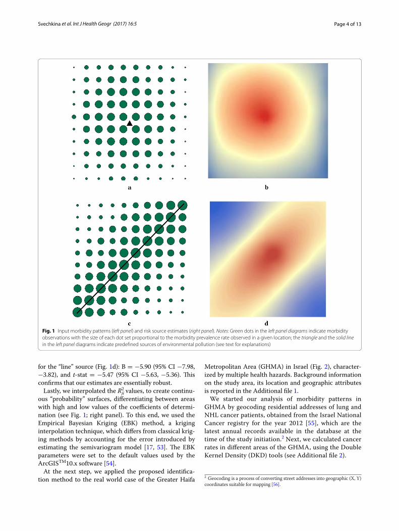
Empirical validationWe tested the proposed identification approach in two stages. During the first stage, we designed several theo-retical examples in which loci of morbidity rates were positioned around pre-defined sources of exposure. In particular, we generated two identical, regularly spaced arrays of 100 “reference” point each, surrounding two pre-defined sources of exposure—either a point or a line (see Fig. 1; left panel). These arrays of “reference” points served in our tests as both disease observations and points from which potential exposure could have been generated. The rates of morbidity were arbitrarily assigned to each refer-ence point using one simple rule: in line with the expected distance decay relationship, reference points with higher morbidity rates were positioned closer to the pre-defined sources of exposure, while places with lower morbidity rates were positioned farther away from these sources (see Fig. 1; left panel). Then, we estimated bivariate regressions to assess the strength of association between morbi and distji for each “reference” point (a total of 100 equations, one for each reference point).

We also incorporated a stochastic element into our analysis. In particular, in order to test the sensitivity of the models under varying levels of inputs, we used a random number generator to generate stochastic noise around the input morbidity rates in our “point” and “line” examples (see Fig. 1). Next, we ran 100 regressions for each of the simulated samples. The test did not change the regres-sion results substantially. In particular, in the case of the “point” source (see Fig. 1b), the estimates for the distance variable were as follows: B  =  −11.17 (95% CI −11.71, −10.63), t-stat = −40.84, (95% CI −41.163, −40.76), and

(6)

Pji → R2ji

(morbi, d̃istji,GEO, SES,POL

), ∀b1 < 0.

Page 4 of 13Svechkina et al. Int J Health Geogr (2017) 16:5

for the “line” source (Fig. 1d): B = −5.90 (95% CI −7.98, −3.82), and t-stat = −5.47 (95% CI −5.63, −5.36). This confirms that our estimates are essentially robust.

Lastly, we interpolated the Rji2 values, to create continu-

ous “probability” surfaces, differentiating between areas with high and low values of the coefficients of determi-nation (see Fig. 1; right panel). To this end, we used the Empirical Bayesian Kriging (EBK) method, a kriging interpolation technique, which differs from classical krig-ing methods by accounting for the error introduced by estimating the semivariogram model [17, 53]. The EBK parameters were set to the default values used by the ArcGISTM10.x software [54].

At the next step, we applied the proposed identifica-tion method to the real world case of the Greater Haifa

Metropolitan Area (GHMA) in Israel (Fig. 2), character-ized by multiple health hazards. Background information on the study area, its location and geographic attributes is reported in the Additional file 1.

We started our analysis of morbidity patterns in GHMA by geocoding residential addresses of lung and NHL cancer patients, obtained from the Israel National Cancer registry for the year 2012 [55], which are the latest annual records available in the database at the time of the study initiation.2 Next, we calculated cancer rates in different areas of the GHMA, using the Double Kernel Density (DKD) tools (see Additional file 2).

2 Geocoding is a process of converting street addresses into geographic (X, Y) coordinates suitable for mapping [56].

Fig. 1 Input morbidity patterns (left panel) and risk source estimates (right panel). Notes: Green dots in the left panel diagrams indicate morbidity observations with the size of each dot set proportional to the morbidity prevalence rate observed in a given location; the triangle and the solid line in the left panel diagrams indicate predefined sources of environmental pollution (see text for explanations)

Page 5 of 13Svechkina et al. Int J Health Geogr (2017) 16:5

In order to convert the obtained continuous DKD surfaces of cancer density into discrete observations, suitable for a multivariate analysis, we generated 1000 randomly distributed “reference” points covering the entire study area (i points). Following the analysis pro-cedure suggested in [11], the reference points created thereby were “spatially joined” with DKD surfaces of both types of cancer under study, enabling us to esti-mate the cancer morbidity rate for each “reference” point. Using the “spatial join” tool in ArcGIS™10.x soft-ware [54], we next assigned the values of several varia-bles, either drawn from small census areas (SCAs) data

(such as socio-economic status, percent of residents employed in manufacturing, the share of total popula-tion over 65yo and neighborhood level smoking rates) or generated from NOx and PM2.5 air pollution sur-faces, to each reference point.

The air pollution surfaces were interpolated by krig-ing using annual averages of air pollution obtained from air quality monitoring stations. According to pre-vious studies, cancer latency period can vary substan-tially, ranging from several years to several decades [57]. To account for this effect, annual averages of NOx and PM2.5, obtained from 20 Air Quality Monitoring

Fig. 2 Map of the GHMA study area, showing residential buildings, main industrial facilities (1–5) and thoroughfare roads

Page 6 of 13Svechkina et al. Int J Health Geogr (2017) 16:5

Stations (AQMSs) [58], were lagged by 10 years, which is a temporal lag, commonly used in epidemiological studies of cancer [59–61]. That is, cancer DKD rates estimated for the year 2013 were mutually compared with air pollution data for the year 2003 (see Appendix 1).

We considered the above mentioned variables as potential confounders for the observed cancer rates, as commonly done in epidemiological studies of cancer morbidity [5, 13, 51, 52]. Descriptive statistics of the vari-ables used in the analysis are reported in “Appendix 1”.

At the next step, we generated a map (layer) of 1000 evenly distributed points, representing locations of potential environmental hazards (j points). For the arrays of i and j, we next calculated Euclidian distances (distji), from each morbidity point (i) to each source points (j). After these distance pairs were calculated, we introduced them into regression models as potential explanatory variables, in addition to the above mentioned socio-demographic and geographic attributes, considered as controls. To address the issue of multicollinearity, indi-vidual distji were introduced into the models separately, one by one, in addition to the constant set of controls, and changes in the coefficient of determinations were traced. The models were estimated separately for two dependent variables—NHL and lung cancer DKD rates.

Because simple Euclidian distances may not be a truly accurate proximity matrix, considering wind frequency and direction, we adjusted these distances by applying a wind frequency transformation discussed in “Appen-dix 2”. By way of this transformation, we calculated wind weighted distances between each pair of i and j

(d̃istji

)

and then used these wind-adjusted distances in the regression analysis as alternatives to simple Euclidean distances, used during the initial phase of the analysis.

Next, for each morbidity reference point (i), we ran multivariate regressions for both types of cancer under study (that is, lung and NHL cancer separately), using the constant set of the above mentioned socio-demo-graphic explanatory and adding one d̃istji at a time. For 1000 multivariate regressions obtained for each type of cancer (that is, one regression equation for each j point), we used the coefficient of determination (R2

ji) to generate the “probability” surface, covering the entire study area and estimating how well the constant set of socio-demo-graphic variables and wind weighted distance from each potential source point j, to the disease observation point i explain cancer rates observed at i’s.

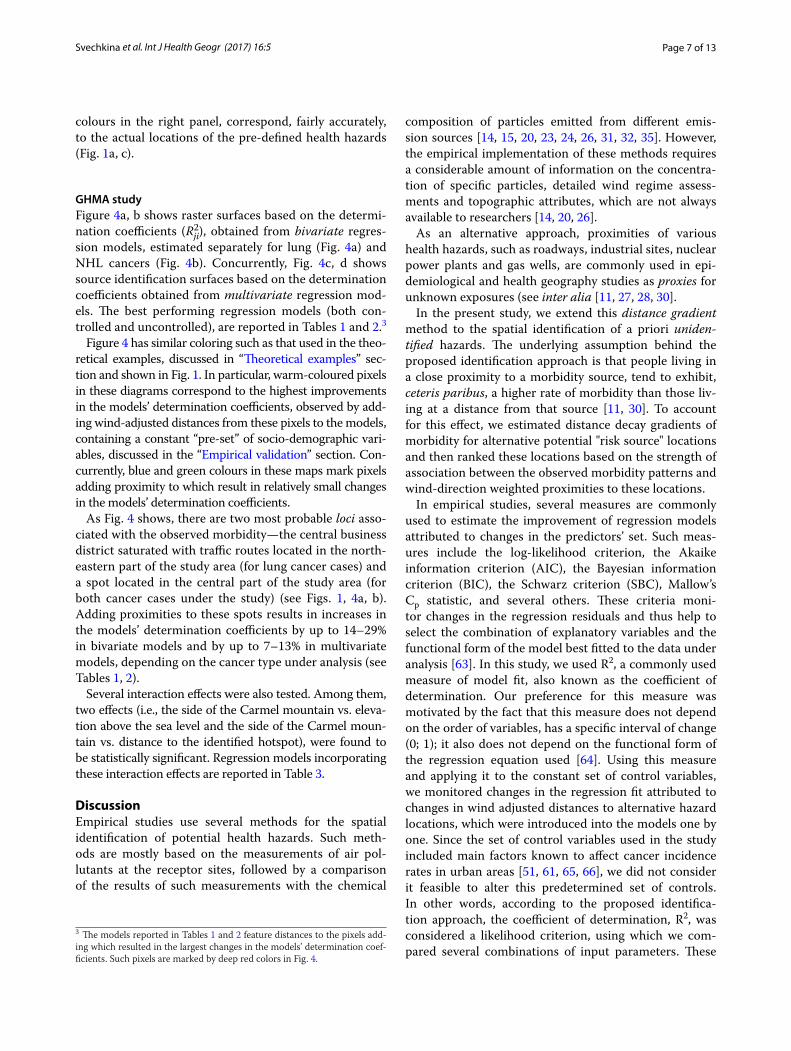
In the initial stage of the analysis, d̃istji were introduced by their linear terms. However, as our analysis revealed, the relationship between the observed cancer morbidity and industrial proximities was best captured by a non-linear (parabolic) function (see Fig.  3), apparently due

to the fact that plumes of air pollution from tall indus-trial smokestacks land at some distances from the emis-sion sources. To take this non-linear effect into account, we introduced a quadratic term of d̃istji into the models, in addition to its linear term, and repeated the analysis. To estimate parameters in Eq. (5) multivariate regression models, incorporating linear and non-linear terms, were used. In the following discussion, only non-linear models, providing better fits and generality compared to ordinary linear models, are reported.

The probability surfaces were generated using the EBK interpolation technique in the ArcGIS™10.x Software [54], while the multivariate regression analysis was per-formed using the SPSSv.23™ software [62]. The probabil-ity level of less than 0.01 (<1%) was set as the accepted statistical significance level.

ResultsTheoretical examplesFigure  1 features morbidity rates, marked by dots sur-rounding two pre-defined sources of exposure—a triangle (Fig. 1a) and a line (Fig. 1c). As mentioned previously, in these diagrams, dots, marking morbidity observations, are sized proportionally to the predefined morbidity rates: the higher the morbidity rate: the bigger the dot that marks it. In line with the expected distance decay relationship, larger dots are positioned closer to the pre-defined sources of exposure, while smaller dots are placed farther away from these sources (see Fig.  1a, c). Concurrently, maps in the right panel (Fig. 1b, d) feature morbidity source estimates, calculated using the estima-tion approach described in  “Empirical validation” sec-tion. As Fig. 1b, d show, the spots of high probability of being the source of exposure, marked by orange and red

0200400600800

1000120014001600

0-10

00

1000

-200

0

2000

-300

0

3000

-400

0

4000

-500

0

5000

-600

0

6000

-700

0

7000

-800

0

8000

-900

0

9000

-100

00

000,001rep,sesacrecnacgnul

dnaLH

N Distance to the industrial facility 5, mNHL Lung

Polynomial fit (NHL) Polynomial fit (Lung)

Fig. 3 Changes in NHL and lung cancer incidence rates (per 100,000) as a function of distance from industrial facility 5 (see Fig. 2)

Page 7 of 13Svechkina et al. Int J Health Geogr (2017) 16:5

colours in the right panel, correspond, fairly accurately, to the actual locations of the pre-defined health hazards (Fig. 1a, c).

GHMA studyFigure 4a, b shows raster surfaces based on the determi-nation coefficients (R2

ji), obtained from bivariate regres-sion models, estimated separately for lung (Fig.  4a) and NHL cancers (Fig.  4b). Concurrently, Fig.  4c, d shows source identification surfaces based on the determination coefficients obtained from multivariate regression mod-els. The best performing regression models (both con-trolled and uncontrolled), are reported in Tables 1 and 2.3

Figure 4 has similar coloring such as that used in the theo-retical examples, discussed in “Theoretical examples” sec-tion and shown in Fig. 1. In particular, warm-coloured pixels in these diagrams correspond to the highest improvements in the models’ determination coefficients, observed by add-ing wind-adjusted distances from these pixels to the models, containing a constant “pre-set” of socio-demographic vari-ables, discussed in the “Empirical validation” section. Con-currently, blue and green colours in these maps mark pixels adding proximity to which result in relatively small changes in the models’ determination coefficients.

As Fig. 4 shows, there are two most probable loci asso-ciated with the observed morbidity—the central business district saturated with traffic routes located in the north-eastern part of the study area (for lung cancer cases) and a spot located in the central part of the study area (for both cancer cases under the study) (see Figs.  1, 4a, b). Adding proximities to these spots results in increases in the models’ determination coefficients by up to 14–29% in bivariate models and by up to 7–13% in multivariate models, depending on the cancer type under analysis (see Tables 1, 2).

Several interaction effects were also tested. Among them, two effects (i.e., the side of the Carmel mountain vs. eleva-tion above the sea level and the side of the Carmel moun-tain vs. distance to the identified hotspot), were found to be statistically significant. Regression models incorporating these interaction effects are reported in Table 3.

DiscussionEmpirical studies use several methods for the spatial identification of potential health hazards. Such meth-ods are mostly based on the measurements of air pol-lutants at the receptor sites, followed by a comparison of the results of such measurements with the chemical

3 The models reported in Tables 1 and 2 feature distances to the pixels add-ing which resulted in the largest changes in the models’ determination coef-ficients. Such pixels are marked by deep red colors in Fig. 4.

composition of particles emitted from different emis-sion sources [14, 15, 20, 23, 24, 26, 31, 32, 35]. However, the empirical implementation of these methods requires a considerable amount of information on the concentra-tion of specific particles, detailed wind regime assess-ments and topographic attributes, which are not always available to researchers [14, 20, 26].

As an alternative approach, proximities of various health hazards, such as roadways, industrial sites, nuclear power plants and gas wells, are commonly used in epi-demiological and health geography studies as proxies for unknown exposures (see inter alia [11, 27, 28, 30].

In the present study, we extend this distance gradient method to the spatial identification of a priori uniden-tified hazards. The underlying assumption behind the proposed identification approach is that people living in a close proximity to a morbidity source, tend to exhibit, ceteris paribus, a higher rate of morbidity than those liv-ing at a distance from that source [11, 30]. To account for this effect, we estimated distance decay gradients of morbidity for alternative potential "risk source" locations and then ranked these locations based on the strength of association between the observed morbidity patterns and wind-direction weighted proximities to these locations.

In empirical studies, several measures are commonly used to estimate the improvement of regression models attributed to changes in the predictors’ set. Such meas-ures include the log-likelihood criterion, the Akaike information criterion  (AIC), the Bayesian information criterion  (BIC), the  Schwarz criterion  (SBC), Mallow’s Cp statistic, and several others. These criteria moni-tor changes in the regression residuals and thus help to select the combination of explanatory variables and the functional form of the model best fitted to the data under analysis [63]. In this study, we used R2, a commonly used measure of model fit, also known as the coefficient of determination. Our preference for this measure was motivated by the fact that this measure does not depend on the order of variables, has a specific interval of change (0; 1); it also does not depend on the functional form of the regression equation used [64]. Using this measure and applying it to the constant set of control variables, we monitored changes in the regression fit attributed to changes in wind adjusted distances to alternative hazard locations, which were introduced into the models one by one. Since the set of control variables used in the study included main factors known to affect cancer incidence rates in urban areas [51, 61, 65, 66], we did not consider it feasible to alter this predetermined set of controls. In other words, according to the proposed identifica-tion approach, the coefficient of determination, R2, was considered a likelihood criterion, using which we com-pared several combinations of input parameters. These

Page 8 of 13Svechkina et al. Int J Health Geogr (2017) 16:5

combinations included the constant set of confound-ers and a number of vectors of wind-weighted distances between alternative potential health risk sources and morbidity observations.

In several theoretical examples we designed, the pro-posed approach helped to identify correctly the prede-fined locations of health hazards, while in a real-world case study, the main health hazard were identified as a spot in the industrial zone, which hosts petrochemical facilities, and a major transportation hub in the cen-tral business district of the city. According to previ-ous studies (see inter alia, [11, 38, 67]), petrochemical industries are known to be associated with evaluated cancer morbidity in surrounding residential areas. In a

separate study, [67] investigated morbidity near nuclear power plants and found it to be linked to childhood cancer.

The results of the present study also correspond to the findings of other studies which revealed geo-graphic concentrations of cancer morbidity near heavy roads [30, 40, 41, 68], and in proximity to industrial areas [11, 38]. Thus, [69] identified the link between traffic-related pollution and respiratory morbidity, measured by lung function impairment.

Several limitations of our study need to be men-tioned. First and foremost, the present study is an ecological analysis, in which explanatory variables are measured at the group level or as distance gradients,

Fig. 4 Risk source assessment for lung cancer (left panel) and NHL cancer (right panel) by uncontrolled (a, b) and controlled regressions (c, d). Note: Black triangles mark the points, distances to which are used in the regression models reported in Tables 1 and 2

Page 9 of 13Svechkina et al. Int J Health Geogr (2017) 16:5

and not estimated for individuals. Therefore, we cannot attribute causality in the relationships we observed. However, the strength of population-level studies is that they represent large population groups and reflect varying levels of exposure. The purpose of such studies is not to prove the relationships but rather to generate hypotheses which can further be examined using individual level data [70].

ConclusionsThis paper contributes to the existing body of literature by extending the traditional distance gradient method (DGM) to the identification of potential health hazards, which geographic location is a priori unknown. The results of the study demonstrate the utility of the pro-posed method for epidemiological studies which goal

is to identify potential sources of exposure to which the observed morbidity is related. We also consider it impor-tant that the proposed approach does not require exten-sive input information and can be used as a preliminary risk assessment tool, helping to identify potential envi-ronmental risk factors behind the observed population morbidity patterns.

The proposed approach can be used by researches worldwide in cases in which specific sources of locally elevated morbidity are unclear or cannot be identified by traditional methods. For instance, the proposed method

Table 1 The association between  double kernel density (DKD) of lung and NHL morbidity rates (cases per 100,000 residents) and  distance to  the revealed exposure sources (Method—bivariate regression, distance variables—linear and quadratic wind-adjusted distance terms)c

Model 1: Bivariate linear model

Model 2: Bivariate quadratic model

* indicates a 0.01 two-tailed significance levela Regression coefficientb t-statistics in the parenthesesc The models reported in the table are estimated for the distances to the “best performing” source locations, marked by small triangles in Fig. 4, that is, source locations distances to which help to improve the models’ fits most significantly (see text for explanations)

Variables Model 1 Model 2Ba and (tb) Ba and (tb)

A. Lung cancer

(Constant) 13.935 (58.947*) 1.131 (7.965*)

Distance −5.500E−0.40 (−19.350*)

0.002 (4.364*)

Distance2 – −1.115E−07 (−4.152*)

No. of reference points

1000 1000

R2 0.286 0.301

R2adjusted

0.285 0.299

F 374.419* 133.819*

B. NHL cancer

(Constant) 4.656 (17.237*) −3.697 (−5.219*)

Distance 3.380E−04 (8.409*) 0.003 (13.916*)

Distance2 – −2.189E−07 (−12.791*)

No. of reference points

1000 1000

R2 0.070 0.205

R2adjusted

0.069 0.204

F 70.714* 120.722*

Table 2 The association between  double kernel den-sity (DKD) of  lung and  NHL morbidity cancer rates (cases per  100,000) and  distance to  the revealed exposure sources (Method—multivariate regression, distance varia-bles—linear and quadratic wind-adjusted distance terms)c

Model 3: Multivariate linear model

Model 4: Multivariate quadratic modela Regression coefficientb t-statistics in the parenthesesc The models reported in the table are estimated for the distances to the “best performing” source locations, marked by small triangles in Fig. 4, that is, source locations distances to which help to improve the models’ fits most significantly (see text for explanations)d The models are controlled for distance to the nearest main road (m), elevation above the sea level (m), percent of Jewish population in the SCA, SCA Socio-economic status, distance to the sea (m), manufacturing employment (% of total population of SCA), NOx (ppb), PM 2.5 (ppb), total population over 65 (%),smoking rate in the SCA (%) and distance to the nearest main road (m)e F-test of R2-change compared to model without hazard source distances (i.e., Models 3A or 3B, respectively)

Variables Model 3d Model 4d

Ba and (tb) Ba and (tb)

A. Lung cancer

(Constant) 6.661 (2.591*) −12.629 (−3.959*)

Distance −5.159E−04 (−7.470*) 0.003 (8.235*)

Distance2 – −2.620E−07 (−8.159*)

N of reference points

1000 1000

R2 0.393 0.458

R2adjusted

0.386 0.450

ΔR2 – 0.065

F changee – 36.658*

B. NHL cancer

(Constant) 9.119 (5.231*) −9.144 (−4.388*)

Distance −2.862E−04 (−5.991*) 0.003 (13.359*)

Distance2 – −2.415E−07 (−12.791*)

N of reference points

1000 1000

R2 0.242 0.369

R2adjusted

0.234 0.361

ΔR2 – 0.127

F changee – 92.855*

Page 10 of 13Svechkina et al. Int J Health Geogr (2017) 16:5

can be used in empirical studies in which available epi-demiological data can help to map the existing morbid-ity patterns, and then to identify potential sources of exposure to which the observed morbidity patterns are related. However, future studies will be needed to extend the theoretical justification of the proposed approach, and to determine its applicability to other urban areas and to other health outcomes.

AbbreviationsCMB: chemical mass balance; DGM: distance gradient method; DKD: double Kernel density method; EBK: empirical Bayesian Kriging; GHMA: greater Haifa metropolitan area; KD: Kernel density; NHL: non-Hodgkin lymphoma cancer; PDF: probability density function; RTA: residence time analysis; SCA: small census area.

Authors’ contributionsMs. Svechkina carried out statistical analysis, performed mapping and drafted the manuscript. Dr. Zusman took part in statistical analysis, designed statistical scripts and assisted with mapping. Ms. Rybnikova helped with data assembling and processing. Prof. Portnov conceived of the study, assisted with

Additional files

Additional file 1. Study area.

Additional file 2. Double kernel density (DKD) estimates.

the study design and implementation and helped to draft the manuscript. All authors read and approved the final manuscript.

AcknowledgementsThe authors express their gratitude to the Israel Center of Disease Control for providing data on cancer morbidity.

Competing interestsThe authors declare no conflict of interests, including personal or financial relationships pertinent to the study.

Availability of data and materials sectionThe datasets supporting the conclusions of this article were obtained from the Israel Center for Disease Control and are not available to general public due to privacy concern.

Consent for publicationAll the authors have read and approved the paper for publication.

Ethics approvalThe study was approved by the University of Haifa’s Ethics Committee (Approval #394/15 dated December 13th, 2015).

FundingThe present study was conducted as a part of the research project, entitled: “Epidemiological monitoring of the Haifa Bay Area: 2015–2020,” funded by the Haifa Municipal Association for Environmental protection (Contract # 45783).

Appendix 1See Table 4.

Table 3 The association between double kernel density (DKD) of lung and NHL morbidity rates (cases per 100,000 resi-dents) and distance to the revealed exposure sources (Method—multivariate regression, distance variables—quadratic wind-adjusted distance terms; interaction terms added)c

See comments to Table 2

Model 5: Multivariate quadratic model with the Side of Mountain Carmel vs. elevation above the sea level interaction term

Model 6: Multivariate quadratic model with the Side of Mountain Carmel vs. Distance to the identified hotspot interaction term

Model 7: Multivariate quadratic model with both interaction terms added

Variables Model 5 Model 6 Model 7Ba and (tb) Ba and (tb) Ba and (tb)

A. Lung cancer

(Constant) −15.663 (−7.937*) −15.125 (−4.832*) −15.791 (−4.948*)

Distance 0.004 (8.591*) 0.004 (9.314*) 0.004 (8.109*)

Distance2 −2.689E−07 (−8.258*) −2.945E−07 (−9.067*) −2.715E−07 (−7.587*)

No. of reference points 1000 1000 1000

R2 0.478 0.480 0.480

R2adjusted

0.470 0.471 0.472

F 56.308* 56.582* 56.790*

B. NHL cancer

(Constant) −9.890 (−4.709*) −9.233 (−4.402*) −10.001 (−4736*)

Distance 0.003 (13.563*) 0.003 (13.119*) 0.003 (12.436*)

Distance2 −2.438E−07 (−12.930*) −2.457 (−11.995*) −2.486E−07 (−11.079*)

No. of reference points 1000 1000 1000

R2 0.373 0.374 0.374

R2adjusted

0.364 0.364 0.364

F 39.311* 39.288* 36.704*

Page 11 of 13Svechkina et al. Int J Health Geogr (2017) 16:5

Appendix 2: Wind weighted transformation of distancesAdjustments for wind frequency and directions were implemented in a number of studies dealing with the measurements of directional concentrations of urban air pollutants (see inter alia, [48, 49, 71, 72]). The empirical literature reports several approaches to distance transfor-mation, based on the seasonal analysis of data [48] or on the amount of precipitation, solar radiation, maximum and minimum temperatures [49] and average wind speed [71].

For the purpose of wind adjustment, we used the wind frequency rose of the study area, plotted at a one-degree angular resolution and showing the average annual dis-tribution of wind frequencies for each one-degree angle. Since the probability of wind from point j to point i (wji) was assumed to be random, we used the probability den-sity function (PDF) instead of a fixed distribution func-tion. PDF describes the relative likelihood for the random variable, e.g., wind frequency to take on a given value (wji):

where wji is annual wind frequency from point j to point i, wj - average annual wind frequency from point j, n - is a number of i points, �j > 0 is the parameter of the distribu-tion, also known as the rate parameter.

Next, distances between j and i (distji) were adjusted for wind frequency and direction as follows:

(7)

PDFw(wji, �j

)= �j · e

−�j ·Wji , ∀Wji ∈ (0, 1),

�j =1

wji, for wj =

1

n

n∑

i=1

wji.

(8)d̃istji = T(distji

∣∣Wji

)= distji · PDF

(Wji, �j

).

According to this transformation, distances between point j and i with frequent winds are reduced, while dis-tances between points with infrequent winds remain unchanged.

Appendix 3 Description of mathematical logic symbols used in the manuscript∀—symbol indicates “for all”, “for any”, “for each”;→—symbol indicates domain and codomain of a

function;∈—symbol indicates affiliation to any set of elements.

Received: 4 August 2016 Accepted: 3 February 2017

References 1. Burkitt DP. Geography of a disease: purpose and possibilities from

geographical medicine. In: Rothschild HR, editor. Biocultural aspects of disease. New York, NY: Academic Press; 1981. pp. 133–51.

2. Pope CA, Dockery DW. Health effects of fine particulate air pollution: lines that connect. J Air Waste Manag Assoc. 2006;56(6):709–42.

3. Kampa M, Castanas E. Human health effects of air pollution. Environ Pol-lut. 2008;151(2):362–7.

4. Chen X, Ye J. When the wind blows: spatial spillover effects of urban air pollution. Environment for Development Discussion: Paper Series 2015; EFD DP 15-15.

5. Cogliano V, Baan R, Straif K, Grosse Y, Lauby-Secretan B, El Ghissassi F, et al. Preventable exposures associated with human cancers. J Natl Cancer Inst. 2011;103(24):1827–39.

6. McKenzie LM, Witter RZ, Newman LS, Adgate JL. Human health risk assessment of air emissions from development of unconventional natural gas resources. Sci Total Environ. 2012;424(1):79–87.

7. Laumbach RJ, Howard MK. Respiratory health effects of air pollution: update on biomass smoke and traffic pollution. J Allergy Clin Immunol. 2012;129(1):3–11.

8. Tuna F, Buluc M. Analysis of PM10 pollutant in Istanbul by using Kriging and IDW methods: between 2003 and 2012. Int J Comput Inf Technol 2015;4(1):170–5.

Table 4 Descriptive statistics of the variables used in the multivariate regressions

Variables Minimum Maximum Mean SD

DKD of NHL cancer cases (per 100,000) 0.00 18.54 6.78 2.49

DKD of Lung cancer cases (per 100,000) 0.00 27.22 10.08 4.04

Average distance to main industrial facilities (m) 755.57 9996.96 5402.55 2095.05

Distance to the nearest main road (m) 0.54 1217.84 163.71 182.13

Distance to the seashore (m) 2.38 14,302.92 4397.48 3872.51

Manufacturing employment (% of total population of the SCA) 0.00 29.30 14.68 6.20

Percent of Jewish population in the SCA 0.00 100.00 91.05 20.54

SCA socio-economic status (Index) −1.62 2.88 0.44 1.08

NOx in 2003 (IDW interpolation, ppb) 7.68 133.12 27.97 15.00

PM2.5 in 2003 (IDW interpolation, ppb) 17.20 27.80 20.11 1.25

Total population over 65 (%) 0.00 0.39 0.17 0.06

Smoking rate in the SCA in 2003 (%) 15.07 41.78 18.87 3.49

Elevation above the sea level (m) 0.00 440.00 110.49 124.83

Page 12 of 13Svechkina et al. Int J Health Geogr (2017) 16:5

9. Ramis R, Gomes-Barroso D, Tamayo I, Garcia-Perez J, Marales A, Romaguera EP, Lopez-Abente G. Spatial analysis of childhood cancer: a case control study. PLoS ONE. 2015;10(5):1–15.

10. Jacquez GM, Greiling DA. Geographic boundaries in breast, lung and colorectal cancers in relation to exposure to air toxics in Long Island, New York. Int J Health Geogr. 2003;2:4.

11. Zusman M, Dubnov J, Barchana M, Portnov BA. Residential proxim-ity of petroleum storage tanks and associated cancer risks: double Kernel density approach vs. zonal estimates. Sci Total Environment. 2012;441:265–76.

12. Portnov BA, Reiser B, Karkabi K, Cohen-Kastel O, Dubnov J. High preva-lence of childhood asthma in Northern Israel is linked to air pollution by particulate matter: evidence from GIS analysis and Bayesian model averaging. Int J Environ Health Res. 2012;22(3):249–69.

13. Hamra GB, Guha N, Cohen A, et al. Outdoor particulate matter expo-sure and lung cancer: a systematic review and meta-analysis. Environ Health Perspect. 2014;122(9):906–11.

14. Cooper JA, Watson JG. Receptor oriented methods of air particulate source apportionment. J Air Pollut Control Assoc. 1980;30(10):1116–24.

15. Stohl A. Trajectory statistics—a new method to establish source-recep-tor relationships of air pollutants and its application to the transport of particulate sulfate in Europe. Atmos Environ. 1996;30(4):579–87.

16. Lupu A, Maenhaunt W. Application and comparison of two statistical trajectory techniques for identification of source regions of atmos-pheric aerosol species. Atmos Environ. 2002;36:5607–18.

17. Pilz J, Spöck G. Why do we need and how should we implement Bayes-ian kriging methods. Stoch Env Res Risk Assess. 2008;22(5):621–32.

18. Zhu L, Huang X, Shi H, Cai X, Song Y. Transport pathways and potential sources of PM10 in Beijing. Atmos Environ. 2011;45:594–604.

19. Singh KP, Gupta S, Rai P. Identifying pollution sources and predicting urban air quality using ensemble learning methods. Atmos Environ. 2013;80:426–37.

20. Cesari R, Paradisi P, Allegrini P. A trajectory statistical method for the identification of sources associated with concentration peak events. Int J Environ Pollut. 2014;55:94–103.

21. Al-Harbi M. Assessment of air quality in two different urban localities. Int J Environ Res. 2014;8(1):15–26.

22. Belis CA, Pernigotti D, Karagulian F, Pirovano G, Larsen BR, Gerboles M, et al. A new methodology to assess the performance and uncertainty of source apportionment models in intercomparison exercises. Atmos Environ. 2015;119:35–44.

23. Salvador P, Artinano B, Alonso DG, Querol X, Alastuey A. Identification and characterisation of sources of PM10 in Madrid (Spain) by statistical methods. Atmos Environ. 2004;38:435–47.

24. Xie Y, Berkowitz CM. The use of positive matrix factorization with conditional probability functions in air quality studies: an applica-tion to hydrocarbon emissions in Houston, Texas. Atmos Environ. 2006;40:3070–91.

25. Wang C, Zhou X, Chen R, Duan X, Kuang X, Kan H. Estimation of the effects of ambient air pollution on life expectancy of urban residents in China. Atmos Environ. 2013;80:347–51.

26. Zhang ZY, Wong MS, Lee KH. Estimation of potential source regions of PM2.5 in Beijing using backward trajectories. Atmos Pollut. 2015;6:173–7.

27. Moore DA, Carpenter TE. Spatial analytical methods and geographic information systems: use in health research and epidemiology. Epidemiol Rev. 1999;20(2):143–61.

28. Rezaeian M, Dunn G, Leger S, Appleby L. Geographical epidemiology, spatial analysis geographical information system: a multidisciplinary glos-sary. J Epidemiol Community Health. 2007;61:98–102.

29. Gatrell AC, Bailey TC, Diggle PJ, Rowlingsont BS. Spatial point pattern analysis and its application in geographical epidemiology. Trans Inst Br Geogr. 1996;21(1):256–74.

30. Paz S, Linn S, Portnov BA, Lazimi A, Futerman B, Barchana M. Non-Hodg-kin Lymphoma (NHL) linkage with residence near heavy roads—a case study from Haifa Bay, Israel. Health Place. 2009;15:636–41.

31. Hopke PK. Recent developments in receptor modelling. J Chemom. 2003;17:255–65.

32. Kim E, Hopke PK. Comparison between conditional probability function and nonparametric regression for fine particle source directions. Atmos Environ. 2004;38:4667–73.

33. Begum BA, Kimb E, Biswasa SK, Hopke PK. Investigation of sources of atmospheric aerosol at urban and semi-urban areas in Bangladesh. Atmos Environ. 2004;38:3025–38.

34. Sacks JD, Ito K, Wilson WE, Neas LM. Impact of covariate models on the assessment of the air pollution-mortality association in a single- and multipollutant context. Am J Epidemiol. 2012;176(7):622–34.

35. Banerjee T, Murari V, Kumar M, Raju MP. Source apportionment of airborne particulates through receptor modelling: Indian scenario. Atmospheric Research 2015; 164–87

36. Pirovano G, Colombi C, Balzarini A, Riva GM, Gianelle V, Lonati G. PM2.5 source apportionment in Lombardy (Italy): comparison of receptor and chemistry-transport modelling results. Atmos Environ. 2015;106:56–70.

37. Johnson S. The ghost map: the story of London’s most terrifying epi-demic—and how it changed science, cities and the modern world 2006; 195–196.

38. Sermage-Faure C, Laurier D, Goujon-Bellec S, Chartier M, Guyot-Goubin A, Rudant J, et al. Childhood leukaemia around French nuclear power plant. The Geocap study, 2002–2007. Int J Cancer. 2012;131(5):E769–80.

39. Yorifuji T, Kashima S. Air pollution: another cause of lung cancer. Lancet Oncol. 2013;14(9):788–9.

40. Su JG, Apte JS, Lipsitt J, Garcia-Gonzales DA, Beckerman BS, Nazelle A, Texcalac-Sangrador JL, Jerrett M. Populations potentially exposed to traffic-related air pollution in seven world cities. Environ Int. 2015;78:82–9.

41. Price K, Plante C, Goudreau S, Boldo EI, Perron S, Smargiassi A. Risk of childhood asthma prevalence attributable to residential proximity to major roads in Montreal, Canada. Can J Public Health. 2012;103(2):113–8.

42. Kim HH, Lee CS, Jeon JM, Yu SD, Lee CW, Park JH, Shin DC, Lim YW. Analy-sis of the association between air pollution and allergic diseases exposure from nearby sources of ambient air pollution within elementary school zones in four Korean cities. Environ Sci Pollut Res. 2013;20(7):4831–46.

43. Houston D, Ong P, Wu J, Winer A. Proximity of licensed child care facilities to near roadway vehicle pollution. Am J Public Health. 2006;96:1611–7.

44. Lumley T. Efficient execution of Stone’s likelihood ratio tests for disease clustering. Comput Stat Data Anal. 1995;20(5):499–510.

45. Tango TA. Class of tests for detecting ‘general’ and ‘focused’ clustering of rare diseases. Stat Med. 1995;14(21–22):2323–34.

46. Bithell JF. The choice of test for detecting raised disease risk near a point source. Stat Med. 1995;14:2309–22.

47. Gatrel A. GIS and health. London; Philadelphia, PA: Taylor & Francis; 1998. 48. Dore AJ, Vieno M, Fournier N, Weston KJ, Sutton MA. Development

of a new wind-rose for the British Isles using radiosonde data, and application to an atmospheric transport model. Q J R Meteorol Soc. 2006;132:2769–84.

49. Chen X, Ye J. When the wind blows: spatial spillover effects of urban air pollution. environment for development discussion: paper series 2015; EFD DP 15–15.

50. Bailey D, Plenys T, Solomon GM, Campbell TR, Feuer GR, Masters J et al. Harboring pollution: strategies to clean up US ports. Natural Resources Defence Council 2004.

51. Anand P, Kunnumakkara AB, Sundaram C, Harikumar KB, Tharakan ST, Lai OS, et al. Cancer is a preventable disease that requires major lifestyle changes. Pharm Res. 2008;25(9):2097–116.

52. Chen H, Goldberg MS, Villeneuve PJ. A systematic review of the relation between long-term exposure to ambient air pollution and chronic diseases. Rev Environ Health. 2008;23(4):243–97.

53. Krivoruchko K. Empirical Bayesian Kriging implemented in ArcGIS Geosta-tistical Analyst. http://www.esri.com (2016). Accessed 10 Feb 2016.

54. ESRI: ArcGIS desktop help 10.2. 2015. http://webhelp.esri.com. Accessed 20 Jan 2015.

55. Ministry of Health (MH): Israel National Cancer Registry. 2012. http://www.health.gov.il. Accessed 10 Feb 2016.

56. Rushton G, Armstrong MP, Gittler J, Greene BR, Pavlik CE, West MM, et al. Geocoding in cancer research: a review. Am J Prev Med. 2006;30(2):16–24.

57. Makimoto Y, Yamamoto S, Takano H et al. Imaging findings of radiation-induced sarcoma of the head and neck. BJR 2014;80(958):790.

58. Israel Ministry of Environmental Protection (IMEP). Map of the air moni-toring stations. 2016. http://www.sviva.gov.il. Accessed 21 Feb 2016.

59. Nyberg F, Gustavsson P, Järup L, Bellander T, Berglind N, Jakobsson R, et al. Urban air pollution and lung cancer in Stockholm. Epidemiology. 2000;11(5):487–95.

Page 13 of 13Svechkina et al. Int J Health Geogr (2017) 16:5

• We accept pre-submission inquiries

• Our selector tool helps you to find the most relevant journal

• We provide round the clock customer support

• Convenient online submission

• Thorough peer review

• Inclusion in PubMed and all major indexing services

• Maximum visibility for your research

Submit your manuscript atwww.biomedcentral.com/submit

Submit your next manuscript to BioMed Central and we will help you at every step:

60. Howard J. Minimum latency and types or categories of cancer. World Trade Center Health Program 2012; 17.

61. Norman RE, Ryan A, Grant K, Sitas F, Scott JG. Environmental contribu-tions to childhood cancers. J Environ Immunol Toxicol. 2014;2(2):86–98.

62. IBM: SPSS Statistics desktop help 22. http://www.ibm.com. Accessed 1 Feb 2016.

63. Burnham KP, Anderson DR. Model selection and multimodel inference: a practical information-theoretic approach. Berlin: Springer; 2002.

64. Baltagi BH. A companion to theoretical econometrics. Malden: Blackwell Publishing Ltd; 2003.

65. Adams RJ, Piantadosi C, Ettridge K, Miller C, Wilson C, Tucker G, Hill C. Functional health literacy mediates the relationship between socio-eco-nomic status, perceptions and lifestyle behaviors related to cancer risk in an Australian population. Patient Educ Couns. 2013;91(2):206–12.

66. Quaglia A, Lillini R, Mamo C, Ivaldi E, Vercelli M. Socio-economic inequali-ties: a review of methodological issues and the relationships with cancer survival. Crit Rev Oncol/Hematol. 2013;85(3):266–77.

67. Spix C, Schmiedel S, Kaatsch P, Schulze-Rath R, Blettner M. Case-control study on childhood cancer in the vicinity of nuclear power plants in Germany 1980–2003. Eur J Cancer. 2008;44(2):275–84.

68. Amram O, Abernethy R, Brauer M, Davies H, Allen RW. Proximity of public elementary schools to major roads in Canadian urban areas. Int J Health Geogr. 2011;10:68–78.

69. Nuvolone D, Maggiore R, Maio S, Fresco R, Baldacci S, Carrozzi L, et al. Geographical information system and environmental epidemiology: a cross-sectional spatial analysis of the effects of traffic-related air pollution on population respiratory health. Environ Health. 2011;10:12.

70. Lindenmayer DB, Likens GE, Andersen A, Bowman DC, Bull M, Bur-nus E, et al. Value of long-term ecological studies. Austral Ecol. 2012;37(7):745–57.

71. Xu X, Akhtar US. Identification of potential regional sources of atmos-pheric total gaseous mercury in Windsor, Ontario, Canada using hybrid receptor modeling. Atmos Chem Phys. 2010;10:7073–83.

72. Zoë L, Fleming ZL, Monks PS, Manning AJ. Review: untangling the influ-ence of air-mass history in interpreting observed atmospheric composi-tion. Atmos Res. 2012;104–105:1–39.

73. Israel Central Bureau of Statistics (ICBS). Statistical abstract of Israel: popu-lation, by population group, religion, sex and age. 2016. http://www.cbs.gov.il/. Accessed 21 Nov 2015.

74. Israel Central Bureau of Statistics (ICBS): Statistical abstract of Israel 2015: population, by district, sub district and religion. 2016. http://www.cbs.gov.il/. Accessed 1 Feb 2016.

75. Bithell JF. An application of density estimation to geographical epidemi-ology. Stat Med. 1990;9:691–701.

76. Shi X. Selection of bandwidth type and adjustment side in kernel density estimation over inhomogeneous backgrounds. Int J Geogr Inf Sci. 2010;24(5):643–60.

77. Portnov BA, Zusman M. Spatial data analysis using kernel density tools. In: Wang J, editor. Encyclopedia of business analytics and optimization. Hershey: Business Science Reference; 2014. p. 2252–64.

78. Kloog I, Haim A, Portnov BA. Using kernel density function as an urban analysis tool: investigating the association between nightlight exposure and the incidence of breast cancer in Haifa, Israel. Comput Environ Urban Syst. 2009;33:55–63.

79. Portnov BA, Dubnov J, Barchana M. Studying the association between air pollution and lung cancer incidence in a large metropolitan area using a kernel density function. Socio-Econ Plan Sci. 2009;43(3):141–50.

80. Zusman M, Broitman D, Portnov BA. Application of the double kernel density approach to the multivariate analysis of attributeless event point dataset. Lett Spatial Resour Sci 2015; 1–20.

81. Silverman BW. Density estimation for statistics and data analysis. London, New York: Chapman and Hall; 1986.

82. Lambe M, Blomqvist P, Bellocco R. Seasonal variation in the diagnosis of cancer: a study based on national cancer registration in Sweden. Br J Cancer. 2003;88(9):1358–60.