Spatial Evolution of Human Dialects - Physics

Spatial Evolution of Human Dialects

James Burridge*

Department of Mathematics, University of Portsmouth, Portsmouth PO1 3HF, United Kingdom(Received 28 February 2017; revised manuscript received 9 May 2017; published 17 July 2017)

The geographical pattern of human dialects is a result of history. Here, we formulate a simple spatialmodel of language change which shows that the final result of this historical evolution may, to some extent,be predictable. The model shows that the boundaries of language dialect regions are controlled by a lengthminimizing effect analogous to surface tension, mediated by variations in population density which caninduce curvature, and by the shape of coastline or similar borders. The predictability of dialect regionsarises because these effects will drive many complex, randomized early states toward one of a smallernumber of stable final configurations. The model is able to reproduce observations and predictions ofdialectologists. These include dialect continua, isogloss bundling, fanning, the wavelike spread of dialectfeatures from cities, and the impact of human movement on the number of dialects that an area can support.The model also provides an analytical form for Séguy’s curve giving the relationship between geographicaland linguistic distance, and a generalization of the curve to account for the presence of a population center.A simple modification allows us to analytically characterize the variation of language use by age in an areaundergoing linguistic change.

DOI: 10.1103/PhysRevX.7.031008 Subject Areas: Complex Systems,Interdisciplinary Physics,Statistical Physics

I. INTRODUCTION

Over time, human societies develop systems of belief,languages, technology, and artistic forms that collectivelymay be called culture. The formation of culture requiresindividuals to have ideas, and then for others to copy them.Historically, most copying has required face-to-face inter-action, and because most human beings tend to remainlocalized in geographical regions that are small in com-parison to the world, human culture can take quite differentforms in different places. One aspect of culture wheregeographical distribution has been studied in great detail isdialect [1].In order to visualize the spatial extent of dialects,

dialectologists have traditionally drawn isoglosses: linesenclosing the domain within which a particular linguisticfeature (a word, a phoneme, or an element of syntax) isused. However, it is not usually the case that language usechanges abruptly at an isogloss—typically there is atransition zone where a mixture of alternative features isused [1]. In fact, there is debate about whether the mostappropriate way to view the geographical organization ofdialects is as a set of distinct areas or as a continuum

without sharp boundaries [1–3]. Whereas an isoglossrepresents the extent of an individual feature, a recogniz-able dialect is typically a combination of many distinctivefeatures [1,4]. We can attempt to distinguish dialects bysuperposing many different isoglosses, but often they donot coincide [3], leading to ambiguous conclusions.The first steps toward an objective, quantitative analysis

of the shapes of dialect areas were made by Séguy [5,6],who examined large aggregates of features, making com-parison between lexical distances and geographic separa-tions. Central to the quantitative study of dialects, calleddialectometry (see Ref. [7] for a recent review), is themeasurement of linguistic distance which, for example, canbe viewed as the smallest number of insertions, deletions,or substitutions of language features needed to transformone segment of speech into another [8]. This “Levenshteindistance” was originally devised to measure the differencebetween sequences [9]. Using a metric of this kind, a set ofdialect observations can be grouped into clusters accordingto their linguistic (as opposed to spatial) closeness [10–13].The clusters then define geographical dialect areas.The question we address is why dialect domains have

particular spatial forms, and to give a quantitative answerrequires a model. The question has been addressed in thepast, famously (amongst dialectologists) by Trudgill andco-workers [1,14], with his “gravity model.” According tothis, the strength of linguistic interaction between twopopulation centers is proportional to the product of theirpopulations, divided by the square of the distance betweenthem. The influence of a settlement (e.g., a city) i on

*[email protected]

Published by the American Physical Society under the terms ofthe Creative Commons Attribution 4.0 International license.Further distribution of this work must maintain attribution tothe author(s) and the published article’s title, journal citation,and DOI.

Selected for a Viewpoint in PhysicsPHYSICAL REVIEW X 7, 031008 (2017)

2160-3308=17=7(3)=031008(27) 031008-1 Published by the American Physical Society

https://doi.org/10.1103/PhysRevX.7.031008




https://creativecommons.org/licenses/by/4.0/

https://creativecommons.org/licenses/by/4.0/

http://link.aps.org/viewpoint-for/10.1103/PhysRevX.7.031008

another j is then defined to be the product of interactionstrength with the ratio Pi=ðPi þ PjÞ, where Pi and Pj arethe population sizes of settlements i and j. These additiveinfluence scores may then be used to predict the progress ofa linguistic change that originated in one city, by determin-ing the settlements over which it exerts the greatest netinfluence. It is then predicted that the change progressesfrom settlement to settlement in a cascade. Predictions mayalso be made regarding the combined influence of cities onneighboring nonurban areas. The model has been partiallysuccessful in predicting observed sequences of linguisticchange [1,15–17], and offers some qualitative insight intothe most likely positions of isoglosses [14]. In this paper,we offer an alternative model, also based on populationdata, which makes use of ideas from statistical mechanics.Rather than starting with a postulate about the nature ofinteractions between population centers, we begin withassumptions about the interactions between speakers. Fromthese assumptions about small-scale behavior we derivepredictions about macroscopic behavior. This approachhas the advantage of making clear the link betweenindividual human interactions and population-level behav-ior. Moreover, we are able to unambiguously define thedynamics of the model and make precise predictions aboutthe locations of isoglosses, the nature of transition regionsbetween linguistic forms, and the most likely structure ofdialect domains. There are links between our approach andagent-based models of language change [18], whichdirectly simulate the behavior of individuals. The differencebetween this approach and ours lies in the fact that for us,assumptions about individual behavior lead to equations forlanguage evolution which are macroscopic in character.These equations have considerable analytical tractabilityand offer a simple and intuitive picture of the large-scalespatial processes at play.In seeking to model the spatial distribution of language

beginning with the individual, we are encouraged by thefact that dialects are created through a vast number ofcomplex interactions between millions of people. Thesepeople are analogous to atoms in the physical context, andwhen very large numbers of particles interact in physicalsystems, simple macroscopic laws often emerge. Despitethe fact that dialects are the product of hundreds of years oflinguistic and cultural evolution [4], and thus historicalevents must have played a role in creating their spatialdistribution [19], the physical analogy suggests that it maybe possible to formulate approximate statistical laws thatplay a powerful role in their spatial evolution.A physical effect analogous to the formation of dialects is

phase ordering [20]. This occurs, for example, in ferromag-netic materials, where each atom attempts to align itself withneighbors. If the material is two dimensional (a flat sheet),this leads to the formation of a patchwork of domains whereall atoms are aligned with others in the same domain, but notwith those in other domains. The boundaries between these

regions of aligned atoms evolve so as to minimize boundarylength [21,22]. The human agents who interact to formdialects behave in roughly the same way (as do some birds[23]). When people speak and listen to each other, they havea tendency to conform to the patterns of speech they hearothers using, and therefore to “align” their dialects. Sincepeople typically remain geographically localized in theireveryday lives, they tend to align with those nearby. Thislocal copying gives rise to dialects in the same way thatshort-range atomic interactions give rise to domains inferromagnets. However, whereas the atoms in a ferromagnetare regularly spaced, human population density is variable.We show that as a result, stable boundaries between domainsbecome curved lines.While our interest is in the spatial distribution of

linguistic forms, there are other properties of languagefor which parallels with the physical or natural world can beusefully drawn, and corresponding mathematical methodsapplied. For example, the rank-frequency distribution ofword use, compiled from millions of books, takes the formof a double power law [24,25], which can be explained [24]using a novel form of the Yule process [26,27], firstintroduced to explain the distribution of the number ofspecies in genera of flowering plants. Historical fluctua-tions in the relative frequency with which words are usedhave been shown to decay as a language ages and expands[25], analogous with the cooling effect produced by theexpansion of a gas. Methods used to understand disorder inphysical systems (“quenched” averages) have been appliedto explain how a tendency to focus on topics controlsfluctuations in the combined vocabulary of groups of texts[28]. A significant focus of current statistical physicsresearch has been on the evolution and properties ofnetworks [29], which have many diverse applications fromthe spread of ideas, fashions, and disease [30] to thevulnerability of the internet [31]. Real networks are oftenformed by “preferential attachment” where new connec-tions are more often made to already well-connected nodes,leading to a “scale-free” (power-law) distribution of nodedegree. The popularity of words has been shown to evolvein the same way [32]; words used more in the past tend tobe used more in the future. Beyond the study of word useand vocabulary, agent-based models such as the naminggame [33], used to investigate the emergence of language,and the utterance selection model [34], used to modelchanges in language use over time, have been particularlyinfluential. We follow the latter model by representinglanguage use using a set of discrete linguistic variables.Spatial models motivated by concepts of statistical physicshave also been used to study the spread of crime [35] and todevise optimal vaccination strategies to prevent disease[36]. The importance of the emergence of order in socialcontexts, and connections to statistical physics, may befound in a wide-ranging review [37] by Castellano et al.

JAMES BURRIDGE PHYS. REV. X 7, 031008 (2017)

031008-2

II. SUMMARY FOR LINGUISTS

A. Contents of the paper

The aim of this paper is to adapt the theory of phaseordering to the study of dialects, and then to use this theoryto explain aspects of their spatial structure. For thosewithout a particular mathematical or quantitative inclina-tion, the model can be simply explained: We assume thatpeople come into linguistic contact predominantly withthose who live within a typical travel radius of their home(around 10–20 km). If they live near a town or city, weassume that they experience more frequent interactionswith people from the city than with those living outside it,simply because there are many more city dwellers withwhom to interact. We represent dialects using a set oflinguistic variables [1], and we suppose that speakers havea tendency to adapt their speech over time in order toconform to local conventions of language use. Our model isdeliberately minimal: these are our only assumptions. Wediscover that, starting from any historical language state,these assumptions lead to the formation of spatial domainswhere particular linguistic variants are in common use, asin Fig. 2. We find that the isoglosses that bound thesedomains are driven away from population centers, that theytend to reduce in curvature over time, and that they are moststable when emerging perpendicular to borders of alinguistic domain. These theoretical principles of isoglossevolution are explained pictorially in Figs. 3, 4, and 5, andprovide a theoretical explanation for a range of observedphenomena, such as the dialects of England (Fig. 7), theRhenish fan (Fig. 10), the wavelike spread of languagefeatures from cities (Figs. 12 and 16), the fact that narrowregions often have “striped” dialects (Fig. 11), and thatcoastal indentations including rivers and estuaries oftengenerate isogloss bundles. Our assumptions also lead to amathematical expression for the relationship betweenlinguistic and geographical distance—the Séguy curve—and a hypothesis regarding the question of when dialectsshould be viewed as a spatial continuum, as opposed todistinct areas (Fig. 19).

B. How might a linguist make use of this work?

Without using mathematics, but having understood ourprinciples of isogloss evolution and considered the exam-ples set out in this paper, further cases may be sought wherethe principles explain observations. If the principles cannotexplain a particular situation or are violated, one might seekto understand what was missing from the underlyingassumptions, or if they were wrong. Since the assumptionsare so minimal, they cannot be the whole story, and adiscussion of possible missing pieces is given in Sec. VIII.For the mathematically inclined linguist, Appendix A setsout an elementary scheme for solving the fundamentalevolution equation on a computer. This scheme also offers asimple and intuitive understanding of the model, and can be

implemented using only a spreadsheet (see SupplementalMaterial [38]), although a computer program would bemuch faster. Using this, isogloss evolution can be exploredin linguistic domains with any shape and populationdistribution. The simplicity of the scheme invites adapta-tion to include more linguistic realism (e.g., bias toward alinguistic variant). Beyond the exploration of individualisoglosses, a line of inquiry that may be of interest todialectometrists is to test our predicted forms of Séguy’scurve against observations.

III. MODEL

Our aim is to define a model of speech copying whichincorporates as few assumptions as possible, whileallowing the effect of local linguistic interaction andmovement to be investigated. The model has its roots inthe ideas of the linguist Bloomfield [3], who believed thatthe speech pattern of an individual constantly evolvedthrough his or her life via pairwise interaction. Thismicroscopic view of language change led to the predictionthat the diffusion of linguistic features should follow routeswith the greatest density of communication. Bloomfielddefined this as the density of conversational links betweenspeakers accumulated over a given period of time. In ourmodel, the analogy of this link density is an interactionkernel weighted by spatial variations in population distri-bution. We implicitly assume that interaction is inherentlylocal so that linguistic changes spread via normal contact[39], rather than via major displacements, conquests,or dispersion of settled communities. We are, therefore,modeling language in stable settlements, with initial con-ditions set by the most recent major population upheaval.We consider a population of speakers, each of whom has

a small home neighborhood, and we introduce a populationdensity ρðx; yÞ giving the spatial variation of the numberhomes per unit area. In order to incorporate local humanmovement within the model, we begin by defining aGaussian interaction kernel for each speaker:

ϕðΔx;ΔyÞ ≔ 1

2πσ2exp

�−Δx2 þ Δy2

2σ2

�:

Note that the symbol ≔ indicates the definition of a newquantity. Consider a speaker, Anna, whose home neighbor-hood is centered on ðx0; y0Þ. In the absence of variation inpopulation density, ϕ is the normalized distribution of therelative positions, ðΔx;ΔyÞ, of the home neighborhoodsof speakers with whom Anna regularly interacts. Theconstant σ, the interaction range, is a measure of the typicalgeographical distance between the neighborhoods of inter-acting speakers. Now suppose that density is not uniformdue to the presence of a city or a sparsely populatedmountainous area. In this case, while Anna is going abouther daily life she is more likely to hold conversations withpeople whose homes lie in a nearby densely populated

SPATIAL EVOLUTION OF HUMAN DIALECTS PHYS. REV. X 7, 031008 (2017)

031008-3

region because these people constitute a greater proportionof the local population. To incorporate this density effect,we define a normalized weighted interaction kernel for ahome at ðx0; y0Þ:

kðx0; y0; x; yÞ ≔ϕðx − x0; y − y0Þρðx; yÞR

R2 ϕðu − x0; v − y0Þρðu; vÞdudv:

Given any regionA, the fraction of Anna’s interactions thatare with people who live in A is

RA kðx0; y0; x; yÞdxdy.

We distinguish between dialects by constructing a set oflinguistic variables whose values vary between dialects. Asingle variable might, for example, be the pronunciation ofthe vowel u in the words “but” and “up” [4]. In England,northerners use a long form, “boott” and “oopp,” withphonetic symbol [℧], and southerners use a short version,[∧]. Considering a single variable which we suppose hasV > 1 variants, we define fiðx; y; tÞ to be the relativefrequency with which the ith variant of our variable is usedby speakers in the neighborhood of ðx; yÞ, at time t. Formathematical simplicity, we assume that nearby speakersuse language in a similar way, so that fiðx; y; tÞ variessmoothly with position.People speak on average 16 000 words per day [40] and

can take months or years (depending on their age andbackground) to adapt their speech to local forms [41,42].Changing speech habits therefore involves a very largenumber of word exchanges, at least in the tens of thousands(comparable in magnitude to typical vocabulary size [43]).Although the rate at which individuals adapt their speech isnot constant throughout life (it is particularly rapid in theyoung), adaptation has been observed even in late middleage [44]. To capture the cumulative effect of linguisticinteraction we make use of a forgetting curve, whichmeasures the relative importance of recent interactions toolder ones. From a mathematical point of view, the simplestform for this curve is an exponential, and in fact there issome evidence from experiments involving word recall[45], which suggests that this is an appropriate choice.However, we emphasize that the curve, for us, is simply away to capture the fact that current speech patterns dependon past interactions and that older interactions tend to beless important. With this in mind we make the followingdefinition of the memory of a speaker from the neighbor-hood of ðx; yÞ, for the ith variant of a variable,

miðx; y; tÞ

≔Z

t

−∞

eðs−tÞ=τ

τ

�ZR2

kðx; y;u; vÞfiðu; v; sÞdudv�ds ð1Þ

≈Z

t

−∞

eðs−tÞ=τ

τ

×

�fiðx; y; sÞ þ

σ2

2ρðx; yÞ∇2fρðx; yÞfiðx; y; sÞg

�ds: ð2Þ

An intuitive understanding of this equation may be gainedby imagining that each speaker possesses an internal taperecorder that records language use as they travel around thevicinity of their home. As time passes, older recordingsfade in importance to the speaker, and the variable mimeasures the historical frequency with which variable i hasbeen heard, accounting for the declining importance ofolder recordings. The rate of this decline is determined bythe parameter τ, which we callmemory length, and note thatchanging its value simply rescales the unit of time. We notealso that this form of memory may be seen as a determin-istic spatial version of the discrete stochastic memory usedin the utterance selection model [34,46]. On the groundsthat speakers collect very large samples of local linguisticinformation, our definition does not contain terms repre-senting random sampling error. In going from Eq. (1) to (2)we use the saddle point method [47] to approximate thespatial integral in Eq. (1) and assume that j∇2ρj=ρ is smallcompared to σ2 (that is, population changes approximatelylinearly over the length scale of human interaction).To allow speakers to base their current speech on what

they have heard in the past, we let fiðx; y; tÞ be a functionpi of the set of memories ðm1; m2;…; mVÞ ≕ m:

fiðx; y; tÞ ≔ pi½mðx; y; tÞ�:

Differentiating Eq. (2) with respect to t, and rescaling theunits of time so that one time unit is equal to one memorylength τ, we obtain

∂miðx; y; tÞ∂t ¼ pi½mðx; y; tÞ� −miðx; y; tÞ

þ σ2

2ρðx; yÞ∇2fρðx; yÞpi½mðx; y; tÞ�g; ð3Þ

which governs the spatial evolution of the ith alternative fora single linguistic variable. We note that memory length nolonger appears as a parameter. An enhanced intuitiveunderstanding of this evolution equation may be gainedfrom its discrete counterpart, used to find computationalsolutions, and derived in Appendix A.The simplest possible choice for pi is to let speakers use

each variant with the same frequency that they remember itbeing used: pi½mðx; y; tÞ� ¼ miðx; y; tÞ. This produces“neutral evolution” [34,46,48–50], where there is no biasin the evolution of each variant. Equation (3) then describespure diffusion, and variants spread out uniformly over thesystem. If all linguistic variables evolved in this way wewould eventually have one spatially homogeneous mixtureof grammar, pronunciation, and vocabulary. If our memorymodel involved a stochastic component [46], then even-tually we would expect all but one variant of each variableto disappear. Neither of these outcomes reflects the realityof locally distinctive forms of language.


031008-4

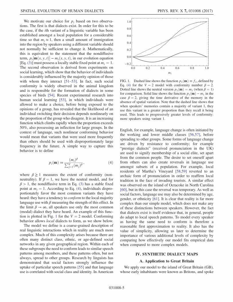
We motivate our choice for pi based on two observa-tions. The first is that dialects exist. In order for this to bethe case, if the ith variant of a linguistic variable has beenestablished amongst a local population for a considerabletime so that mi ≈ 1, then a small amount of immigrationinto the region by speakers using a different variable shouldnot normally be sufficient to change it. Mathematically,this is equivalent to the statement that the nondiffusiveterm, pi½mðx; y; tÞ� −miðx; y; tÞ, in our evolution equation[Eq. (3)] must possess a locally stable fixed point atmi ¼ 1.The second observation is derived from experiments onsocial learning, which show that the behavior of individualsis considerably influenced by the majority opinion of thosewith whom they interact [51–53]. In fact, such socialconformity is widely observed in the animal kingdomand is responsible for the formation of dialects in somespecies of birds [54]. Recent experimental research intohuman social learning [53], in which individuals wereallowed to make a choice, before being exposed to theopinions of a group, has revealed that the likelihood of anindividual switching their decision depends nonlinearly onthe proportion of the group who disagree. It is an increasingfunction which climbs rapidly when the proportion exceeds50%, also possessing an inflection for large groups. In thecontext of language, such nonlinear conforming behaviorwould mean that variants that were used more frequentlythan others should be used with disproportionately largefrequency in the future. A simple way to capture thisbehavior is to define

piðmÞ ≔ ðmiÞβPVj¼1ðmjÞβ

; ð4Þ

where β ≥ 1 measures the extent of conformity (non-neutrality). If β ¼ 1, we have the neutral model, and forβ > 1, the nondiffusive term in Eq. (3) has a stable fixedpoint at mi ¼ 1. According to Eq. (4), individuals dispro-portionately favor the most common variants they haveheard: they have a tendency to conform to the local majoritylanguage use with β measuring the strength of this effect. Inthe limit β → ∞, all speakers use only the most common(modal) dialect they have heard. An example of this func-tion is plotted in Fig. 1 for the V ¼ 2 model. Conformingbehavior allows local dialects to form, as we show below.The model we define is a coarse-grained description of

real linguistic interactions which in reality are much morecomplex. Much of this complexity arises because there areoften many distinct class, ethnic, or age-defined socialnetworks in any given geographical region. Within each ofthese subgroups the need to conform leads to similar speechpatterns among members, and these patterns often, but notalways, spread to other groups. Research by linguists hasdemonstrated that social factors strongly influence theuptake of particular speech patterns [55] and that languageuse is correlated with social class and identity. In American

English, for example, language change is often initiated bythe working and lower middle classes [56,57], beforespreading to other groups. Some forms of language changeare driven by resistance to conformity; for example“prestige dialects” (received pronunciation in the UK)are used to signify membership of a social elite, set apartfrom the common people. The desire to set oneself apartfrom others can also create reversals in language useamongst subsets of a population. For example, localresidents of Martha’s Vineyard [58,59] reverted to anarchaic form of pronunciation in order to reaffirm localtradition in the face of invading tourists. A similar effectwas observed on the island of Ocracoke in North Carolina[60], but in this case the reversal was temporary. As well associal factors, language use may also be determined by age,gender, or ethnicity [61]. It is clear that reality is far morecomplex than our simple model, which does not make anyof these distinctions between speakers. However, the factthat dialects exist is itself evidence that, in general, peopledo adapt to local speech patterns. To model every speakeras having the same need to conform is therefore areasonable first approximation to reality. It also has thevalue of simplicity, allowing us later to determine theimportance of various additional levels of complexity bycomparing how effectively our model fits empirical datawhen compared to more complex models.

IV. SYNTHETIC DIALECT MAPS

A. Application to Great Britain

We apply our model to the island of Great Britain (GB),whose early inhabitants were known as Britons, and spoke

FIG. 1. Dashed line shows the function p1ðmÞ≡ f1, defined byEq. (4) for the V ¼ 2 model with conformity number β ¼ 2.Dotted line shows the neutral version p1ðmÞ ¼ m1 (when β ¼ 1)for comparison. Solid line shows the function p1ðmÞ −m1 in thecase β ¼ 2, giving the time derivative of the memory in theabsence of spatial variation. Note that the dashed line shows thatwhen speakers’ memories contain a majority of variant 1, theyuse this variant in a greater proportion than they recall it beingused. This leads to progressively greater levels of conformity:more speakers using variant 1.


031008-5

Celtic languages [62]. The earliest form of English wasbrought to the island by invading Germanic-speakingsettlers. This became Anglo Saxon (or Old English), aswritten by Alfred, King of Wessex (849–899 A.D.), butwould not be recognizable to modern speakers. It slowlychanged, with external influences (notably Norman), intothe English we know today [19].We seek to discover the extent to which the spatial

distribution of dialect structures that have emerged in GBcan be predicted by Eq. (3). To model the evolution ofindividual linguistic variables we take mainland GB as ourspatial domain, and numerically solve Eq. (3) on a grid ofdiscrete points (Fig. 2) using an explicit Euler scheme [63](Appendix A). The initial condition for the solution is arandomly generated spatial frequency distribution whereeach grid point is assigned a randomly selected variant. Byrepeatedly generating initial conditions and solving thesystem, we can determine the most probable equilibriumspatial distributions of language use. The populationdensity ρðx; yÞ is estimated using 2011 census data [64],which gives the number of inhabitants at each of the ≈1.8 ×106 UK postcodes. A smooth density is then obtained fromthis by allowing the inhabitants to diffuse a short distancefrom the geographical center of their postcode. Despitesignificant overall population growth, the locations ofmajor population centers in GB can trace their origins

back through hundreds of years. Since dialect evolutionequation (3) depends only on relative population densities,the current density distribution therefore serves as reason-able proxy for historical versions. We estimate that σ lies inthe range 5 < σ < 15 km based on that fact that theaverage distance traveled to work in GB in 2011 was15 km [64], whereas the average distance traveled tosecondary school was 5.5 km [65]. In Sec, VII, we findthat the typical width of a transition region betweenlinguistic variables is ≈1.8σðβ − 1Þ−1=2. For example, thetransition between northern and southern GB dialects is≈60 km wide [1], which, if σ ¼ 10 km, gives the approxi-mation β ≈ 1.1.

1. Evolution of isoglosses

When it comes to interpreting our results, the fact thatusage frequencies are continuously varying through spacepresents a similar problem to that faced by dialectologistswhen trying to draw isoglosses. We resolve this by definingdomain boundaries to be lines across which the modal(most common) variant changes. A domain is therefore aregion throughout which a single variant is the mostcommonly used. We may think of domain boundaries assynthetic isoglosses generated by Eq. (3). In Fig. 2, weshow a series of snapshots of the evolution of domainswhen there are V ¼ 3 variants. Isogloss evolution is drivenby a two-dimensional form of surface tension [66]: in theabsence of density variation, curved boundaries straightenout. Figure 3 illustrates why this happens faster whencurvature is greater. Here, speaker L hears more of variantA, so domain B will retract in this locality. Speaker R hearsmore of variant B, and so domain A will retract in thisregion. The net effect will be to straighten the boundary,reducing its length. If a boundary forms a closed curve,then this length reduction effect can cause it to evolvetoward a circular shape, and reduce in area, eventuallydisappearing altogether. However, this shrinking dropleteffect can be arrested or reversed if the droplet surrounds asufficiently dense population center (a city). In fact,population centers typically repel isoglosses in our model,and so have a tendency to create their own domains. Anexplanation of this effect is given in Fig. 4. Here, we have a

FIG. 2. Evolution of the V ¼ 3 model from randomizedinitial condition with σ ¼ 15 km and β ¼ 1.1 at timest ∈ f1; 2; 4; 8; 16; 32g, where one time unit corresponds to onememory length. Colors indicate which variant is most common ateach position. Numerical solution implemented in C++ on gridwith 2-km spacing [63] (GB is ≈1000 km north to south). Eachgrid point initialized with randomly selected variant.

FIG. 3. The surface tension effect at domain boundaries. Bluedots represent speakers and black circles give an approximaterepresentation of interaction ranges. In the red shaded parts ofthese interaction ranges, variant A is more common, and in theyellow shaded parts, variant B is more common.


031008-6

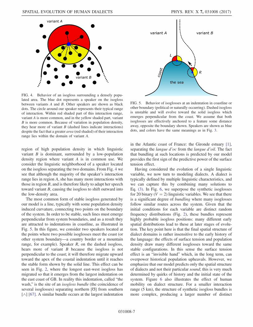
region of high population density in which linguisticvariant B is dominant, surrounded by a low-populationdensity region where variant A is in common use. Weconsider the linguistic neighborhood of a speaker locatedon the isogloss separating the two domains. From Fig. 4 wesee that although the majority of the speaker’s interactionrange lies in region A, she has many more interactions withthose in region B, and is therefore likely to adapt her speechtoward variant B, causing the isogloss to shift outward intothe low-density area.The most common form of stable isogloss generated by

our model is a line, typically with some population densityinduced curvature, connecting two points on the boundaryof the system. In order to be stable, such lines must emergeperpendicular from system boundaries, and as a result theyare attracted to indentations in coastline, as illustrated inFig. 5. In this figure, we consider two speakers located atthe points where two possible isoglosses meet the coast (orother system boundary—a country border or a mountainrange, for example). Speaker R, on the dashed isogloss,hears more of variant B because the isogloss is notperpendicular to the coast; it will therefore migrate upwardtoward the apex of the coastal indentation until it reachesthe stable form shown by the solid line. This effect can beseen in Fig. 2, where the longest east-west isogloss hasmigrated so that it emerges from the largest indentation onthe east coast of GB. In reality this indentation, called “thewash,” is the site of an isogloss bundle (the coincidence ofseveral isoglosses) separating northern [℧] from southern[∧] [67]. A similar bundle occurs at the largest indentation

in the Atlantic coast of France: the Gironde estuary [1],separating the langue d’oc from the langue d’oil. The factthat bundling at such locations is predicted by our modelprovides the first sign of the predictive power of the surfacetension effect.Having considered the evolution of a single linguistic

variable, we now turn to modeling dialects. A dialect istypically defined by multiple linguistic characteristics, andwe can capture this by combining many solutions toEq. (3). In Fig. 6, we superpose the synthetic isoglossesfor 20 binary (V ¼ 2) linguistic variables. We see that thereis a significant degree of bundling where many isoglossesfollow similar routes across the system. Given that theinitial conditions for each variable are distinct randomfrequency distributions (Fig. 2), these bundles representhighly probable isogloss positions: many different earlyspatial distributions lead to these at later stages of evolu-tion. The key point here is that the final spatial structure ofdialect domains is rather insensitive to the early history ofthe language: the effects of surface tension and populationdensity draw many different isoglosses toward the samestable configurations. In this sense the surface tensioneffect is an “invisible hand” which, in the long term, canoverpower historical population upheavals. However, weemphasize that our model predicts only the spatial structureof dialects and not their particular sound; this is very muchdetermined by quirks of history and the initial state of thesystem. Figure 6 also illustrates the effect of humanmobility on dialect structure. For a smaller interactionrange (5 km), the structure of synthetic isogloss bundles ismore complex, producing a larger number of distinct

FIG. 4. Behavior of an isogloss surrounding a densely popu-lated area. The blue dot represents a speaker on the isoglossbetween variants A and B. Other speakers are shown as blackdots. The circle around our speaker represents their typical rangeof interaction. Within red shaded part of this interaction range,variant A is more common, and in the yellow shaded part, variantB is more common. Because of variation in population density,they hear more of variant B (dashed lines indicate interactions)despite the fact that a greater area (red shaded) of their interactionrange lies within the domain of variant A.

FIG. 5. Behavior of isoglosses at an indentation in coastline orother boundary (political or naturally occurring). Dashed isoglossis unstable and will evolve toward the solid isogloss whichemerges perpendicular from the coast. We assume that bothisoglosses are effectively anchored to a feature some distanceaway, opposite the boundary shown. Speakers are shown as bluedots, and colors have the same meanings as in Fig. 3.


031008-7

regions. This effect is well documented in studies of thehistorical evolution of dialects which were, in the past,more numerous and covered smaller geographical areas [4].Within our model, this is explained by the fact thatfluctuations in population density become relevant toisogloss evolution only when they take place over a lengthscale that is comparable to the interaction range: Twohuman settlements could develop distinct dialects only ifthey were separated by a distance significantly greater thanσ, otherwise they would be in regular linguistic contact.

2. Cluster analysis

Having analyzed our model using isoglosses, we nowmake comparison to recent work in dialectometry, wheredialect domains have been determined using clusteranalysis and by multidimensional scaling [68]. A typicalclustering approach [10,12] is to construct a data set givingthe frequencies of a wide range of variant pronunciations atdifferent locations, and then to cluster these locationsaccording to the similarity of their aggregated sets ofcharacteristics. Resampling techniques such as bootstrap[69] may be used to generate “fictitious” data sets andimprove stability. We mimic this approach by constructinga synthetic data set from 20 solutions of Eq. (3) with V ¼ 2,and each with different random initial conditions, corre-sponding to different linguistic variables. We then ran-domly select a large number (6000) of sample locationswithin GB and determine the modal variants for each of the20 variables at each location. This sample size is chosen tobe sufficiently large so that the effect of resampling is onlyto make short length scale (≪1 km) changes to cluster

boundaries. These aggregated data are then divided into kclusters using the k-medoids algorithm [70] (available inthe R language). The metric used for linguistic distancebetween sample points is the Manhattan distance betweenthe binary vectors, where the two variants are labeled 1 or−1. Because we are comparing vectors which can betransformed into one another purely by substitutions(1 for −1 or vice versa), rather than insertions or deletions,this is equivalent to the Levenshtein distance used indialectometry [2,9]. We find that almost identical resultsare obtained by applying Ward’s hierarchical clusteringalgorithm [71] to the sample locations and subsequentlycutting the tree into k clusters.In order to compare our cluster analysis to the work of

dialectologists, we consider a prediction for the futuredialect areas of England (excluding Wales and Scotland)made by Trudgill [4], shown in the left-hand map of Figs. 7and 8. This prediction divides the country into 13 regions,and is the result of a systematic analysis of regionalvariation in speech and ongoing changes. Such sharp

FIG. 6. Superposition of the isoglosses at t ¼ 50 produced by20 solutions of the V ¼ 2model with β ¼ 1.1, each with differentrandomized initial conditions. For the left-hand map, σ ¼ 5 km,and for the right-hand map, σ ¼ 10 km (see video in Supple-mental Material [38]). Background shading indicates populationdensity with brightest orange corresponding to 7200 inhabitantsper km2.

FIG. 7. Left map: Future England dialect boundaries predictedby Trudgill [4]. Right map: Future dialect boundaries predictedusing k-medoids cluster analysis of 20 synthetic binary linguisticvariables when σ ¼ 10 km and β ¼ 1.1 at t ¼ 150. Levenshteindistance (or “edit distance”) [9] used as distance metric. Colors,determined by Hungarian method, show mapping betweendialect areas. Black dotted line shows north-south isogloss.

FIG. 8. Left map: Future England dialect boundaries predictedby Trudgill [4]. Right map: Voronoi tessellation with the samenumber of cells as Trudgill’s prediction. Colors determined byHungarian algorithm.


031008-8

divisions are a significant simplification of reality, however,and hide many subtle smaller-scale variations. The decisionto define 13 regions therefore reflects a judgment on therange of language use which can be categorized as a singledialect. To allow comparison with this prediction, weperform a set of cluster analyses of near-equilibrium(large t) solutions for the whole of GB, for a range ofvalues of the number k of clusters (see Fig. 9), with theaim of producing 13 within the subset of GB defined byEngland. The closest result is 14 clusters for 20 ≤ k ≤ 24,with almost identical results within England for each ofthese choices. Having defined our synthetic dialect regions,we apply the Hungarian method [72] to find the mappingbetween our synthetic dialects and Trudgill’s predicteddialects, which maximizes the total area of overlap betweenthe two. The results are shown in Fig. 7. To provide ameasure of the effectiveness of our model in matchingTrudgill’s predictions, we also define a null model, whichdivides the country into regions at random, independent ofpopulation distribution and without reference to any modelof speaker interaction. There are a number of models thatgenerate random tessellations of space [73], many of whichare motivated by physical processes such as fracture orcrack propagation. We exclude such physical assumptionand thus opt for the Voronoi tessellation [73], based on thePoisson point process: the simplest of all random spatialprocesses. Our null model is then a Voronoi tessellation ofEngland (Fig. 8) using 13 points selected uniformly atrandom from within its borders, with dialects labeled tomost closely match Trudgill’s map, using the Hungarianmethod.Having generated our synthetic dialect maps, we now

quantify the extent to which they match the predictions ofTrudgill. The null model, because of its lack of modelingassumptions, will reveal the extent to which our model is“better than random” at matching these predictions. Weoffer four alternative metrics of similarity in Table I. Thesimplest metric is overlap (OL): the percentage of land areawhich is identified as belonging to the same dialect as

Trudgill’s prediction. The weighted overlap (WOL)weights overlapping regions in proportion to their popu-lation density: it gives the probability that a randomlyselected inhabitant will be assigned to the same dialect zoneby both maps. From Table I we see that this probability ishigh (82%) for our model, but lower for the randomVoronoi model. We suggest that this is a result of the factthat population centers tend to repel isoglosses and,therefore, often lie at the centers of dialect domains. Weexamine this repulsion effect in more detail below. Thefinal two metrics are commonly used to compare cluster-ings. Consider a set S of elements (spatial locations for us)that has been partitioned into clusters (dialect areas) in twodifferent ways. Let us call these two partitions X and Y. TheRand index (RI) [74] is defined as the probability that,given two randomly selected elements of S, the partitions Xand Y will agree in their answer to the question: are bothelements in the same cluster? A disadvantage with usingthis index to compare dialect maps is that the larger thenumber of regions in the maps, the more likely it is that tworandomly selected spatial points will not lie in the samecluster in either map. The index therefore approaches 1 asthe number of dialect areas grows. This problem may becountered by taking account of its expected value if X andY were picked at random, subject to having the samenumber of clusters and cluster sizes as the originals [75].The “adjusted Rand index” (ARI) is then defined as

ARI ≔RI − expected index1 − expected index

: ð5Þ

The ARI ∈ ½−1; 1� measures the extent to which a cluster-ing is a better match than random to some referenceclustering and is used by dialectometrists [76] in preferenceto the original Rand index. For us, the reference clusteringis Trudgill’s predicted dialect map, and the Rand andadjusted Rand indices in Table I measure similarity to thisreference.The primary conclusion that may be drawn from the

indices in Table I is that by all measures our model provides

FIG. 9. Results of k-medoids cluster analysis of 20 syntheticbinary linguistic variables when σ ¼ 10 km and β ¼ 1.1 att ¼ 150. Edit distance [9] used as distance metric. k values fromleft to right are k ¼ 16, 22, 30.

TABLE I. Metrics measuring the similarity between Trudgill’spredictions [4] for future English dialects and the predictions ofour model. Metric acronyms are OL (overlap), WOL (weightedoverlap), RI (Rand index), and ARI (adjusted Rand index). TheVoronoi example column gives equivalent metrics for theexample Voronoi tessellation in Fig. 8, and the Voronoi setcolumn gives the mean metrics, with standard deviation, for fiverandomly generated Vornoi tessellations.

Metric Model Voronoi example Voronoi set

OL 68% 41% 45� 3%WOL 82% 36% 49� 11%RI 0.91 0.84 0.83� 0.01ARI 0.63 0.29 0.30� 0.01


031008-9

a better match than the null model (indices all differ by atleast 3 standard deviations, and typically many more). Ofparticular interest is the weighted overlap probability(WOL ¼ 82%). Isoglosses are typically repelled by pop-ulation centers, so tend to pass through regions of relativelylow density. Because of this the WOL may be viewed as ameasure of the effectiveness of the model at determiningthe centers of dialect regions and is less sensitive to smallerrors in isogloss construction, explaining its high value. Itis important to realize also that Trudgill’s predictions maythemselves be imperfect.We now make some qualitative comments. The dotted

line in Fig. 7 shows the location of our model’s most densenorth-south isogloss bundle. This is coincident with what isdescribed by Trudgill as “one of the most importantisoglosses in England” [14] dividing those who have [℧]in butter from those who do not. In our model, the fact thatthis border lies where it does is a result of the surfacetension effect which attracts many isoglosses towards thetwo coastal indentations at either end (see video inSupplemental Material [38]). The fact that many random-ized initial boundary shapes evolve toward this configura-tion, and that the configuration is seen as important bydialectologists, supports the hypothesis that surface tensionis an important driver of spatial language evolution. Wealso note that the western extremities of GB (Cornwall andnorthwest Scotland) support multiple synthetic dialects inour model, and we suggest that this is due to a heavilyindented coastline and the fact that high aspect-ratiotongues of land are likely to be crossed by isoglosses; afact predictable by analogy with continuum percolation[21]. The southwest peninsula has historically supportedthree dialects.In future work, the model might be tested by comparing

its predictions to well-researched dialect areas. On exampleis Netherlands. Here, dialectologists have performed acluster analysis [68] based on Levenshtein distancesbetween field observations of 360 dialect varieties (corre-sponding to 357 geographical locations), revealing 13significant geographical groupings. The extent to whicha model is consistent with these groupings, accounting forvariability caused by finite sample size, could be tested bygenerating equivalent clusterings for multiple fictitiousdialect samples of the same size.

B. Bundles, fans, stripes, and circular waves

We now illustrate a number of well-known features ofdialect distributions which may be qualitatively reproducedby our model. We consider first the isogloss bundlereported by Bloomfield [3] separating “High German”from “Low German.” The bundle emerged from the tipof an indentation of the Dutch-German speech area(bordered to the east by Slavic languages) and ran roughlyeast-west before separating approximately 40 km east ofthe river Rhine, and fanning out around cities such as

Dusseldorf, Cologne, Koblenz, and Trier. This arrangementof isoglosses is known as the “Rhenish fan.” In Fig. 10, weconstruct an artificial system with boundaries approximat-ing the geographical structure of relevant parts of theDutch-German language area illustrated in Bloomfield[3] containing an artificial cluster of population centersrepresenting the German cities located near the Rhine. Thesystem was initialized using the same randomizationprocedure used for GB, and Fig. 10 shows a superpositionof ten solutions, each with different initial conditions. In theearly stages of evolution, very little pattern is discernible,but as time progresses, the main indentation collectsisoglosses, while the cities repel them, producing a fanlikestructure. We therefore suggest that the isogloss separationwhich created the Rhenish fan may have been the result ofrepulsion by the cities of the Rhine.We next consider an example of what some physicists

refer to as “stripe states” [21]: in finite systems thatexperience phase ordering, and have aspect ratios greaterthan 1, boundaries between two orderings often form acrossthe system by the shortest route (in a rectangle, joining twolong sides). A collection of such boundaries forms a stripedpattern of phase orderings. Figure 11 illustrates this effect,produced by Eq. (3). Our model therefore predicts suchstriped dialect patterns in long thin countries, and aparticularly striking example of the effect may be seenin the dialects of the Saami language [77]. The Saamipeople are indigenous to the Sámpi region (Lapland),which includes parts of Norway, Sweden, and Finland.Their Arctic homeland forms a curved strip with a lengthwhich is approximately 5 times its average width. Theregion is divided into ten language areas, and the bounda-ries of all but two of these take a near-direct route betweenthe two long boundaries of the system, forming a distinctivestriped pattern. Another example is the dialects of Japan,

FIG. 10. Evolution of isoglosses in a 400 × 200 system with twoopposing boundary indentations and unit background populationdensity, together with a collection of cities contributing additionalpopulation densities ρðrÞ ¼ ðρ1 − 1Þ exp f−r2=ð2R2Þg, where r isdistance from city center, R ¼ 10, and ρ1 ¼ 4 (measuring ratio ofpeak city density to background). Parameter values σ ¼ 4, β ¼ 2.Evolution times t ¼ 10, 50, 300, 1660. See video in SupplementalMaterial for full animation [38].


031008-10

whose boundaries in many cases cross the countryperpendicular to its spine [78].The relationship between geographical separation and

linguistic distance (often measured using Levenshtein dis-tances [2]) is typically sublinear [2,39]. The definition oflinguistic distance and its relation to geographic distancewas made by Séguy [5,6], and the relationship thereforegoes by the name Séguy’s curve [39]. It has beensubstantially refined and tested since [2,39,79], and alsogeneralized to involve travel time [80]. Séguy’s curve is notuniversal, however. For example, an analysis of Tuscandialect data [81] reveals an unusually low correlationbetween phonetic and geographical distances. A moredetailed analysis reveals that there are geographicallyremote areas which are linguistically similar, and thatwithin an approximately circular region (radius ≈40 km)around the main city, Florence, phonetic variation corre-lates more strongly with geographical proximity. It ishypothesized [81] that this pattern marks the radial spreadof a linguistic innovation (called “Tuscan-gorgia”). TheseTuscan data motivate our final example of the qualitativebehavior of our model. To illustrate how a linguisticvariable can spread outwards from a population center,purely through the effects of population distribution and notnecessarily driven by prestige or other forms of bias, wesimulate our model using an artificial city with Gaussianpopulation distribution (Fig. 12). The system is initializedwith a circular isogloss, centered on the city, representing alocal linguistic innovation. Because population density is adecreasing function of the distance from the city center,speakers on the isogloss hear more of the innovation thantheir current speech form, allowing it to expand (asexplained in Fig, 4). We see in Sec. VII that this expansionwill not not necessarily continue indefinitely. Expansionprocesses such as this have also been observed in Norway[14]. In that case, the progress of new linguistic forms wasshown to depend on age, with changes more advanced for

younger speakers, who are more susceptible to new formsof speech. We illustrate how this effect can be analyzed inAppendix B.

V. SÉGUY’S CURVE

We now determine the relationship between geographi-cal and linguistic distance within our model, providing ananalytical prediction for the form of Séguy’s curve [5,6,39].For simplicity, we consider the two variant model V ¼ 2and suppose that our language contains a number n oflinguistic variables. At each location in space the localdialect is an n-dimensional vector of the local modalvariants which we label 1 and −1. Letting ϕðr; tÞ, wherer ¼ ðx; yÞ, be the vector field giving the distribution ofthese variants, the number of differences (the Levenshteindistance [9]) between two dialects ϕðr1; tÞ ≕ ϕð1Þ andϕðr2; tÞ ≕ ϕð2Þ is ½n − ϕð1Þ · ϕð2Þ�=2. The linguistic dis-tance Lð1; 2Þ between two dialects may be defined [82] asthe fraction of variables that differ between them:

Lð1; 2Þ ≔ 1

2

�1 −

ϕð1Þ · ϕð2Þn

�: ð6Þ

Since we assume that each variant evolves independently ofevery other, the expected linguistic distance is

lð1; 2Þ ≔ E½Lð1; 2Þ� ¼ 1

2ð1 −E½ϕið1Þϕið2Þ�Þ; ð7Þ

where ϕi is the ith component of ϕ. To computeE½ϕið1Þϕið2Þ�, we make use of the close similarity between

FIG. 11. Evolution of isoglosses in a 400 × 200 rectangularsystem with uniform population density, starting from random-ized initial conditions. We show a superposition of 10 suchsolutions. Notice that all isoglosses join the two long sides of thesystem. Parameter values σ ¼ 4, β ¼ 2. Evolution times t ¼ 30,90, 270, 810.

FIG. 12. Evolution of a circular isogloss (initial radius 30) in a200 × 200 system with unit background population density,together with a central city contributing additional densityρðrÞ ¼ ðρ1 − 1Þ exp f−r2=ð2R2Þg, where r is distance from citycenter, R ¼ 40, and ρ1 ¼ 21. Parameter values σ ¼ 4, β ¼ 2.Evolution times t ∈ f10; 20; 30;…; 300g.


031008-11

Eq. (3) and the time-dependent Ginzburg-Landau equation[20] to derive (see Appendix C) an analogue of the Allen-Cahn equation [83] giving the velocity of an isogloss at apoint in terms of the unit vector g normal to it at that point:

v ¼ −βσ2�∇ · g

2þ∇ρ · g

ρ

�ð8Þ

¼ −βσ2�κ

2þ∇ρ · g

ρ

�: ð9Þ

The quantity κ is the curvature of the isogloss at the point:in the absence of variations of population density, theisogloss moves so as to reduce curvature. The second termin the square brackets produces a net migration of iso-glosses towards regions of lower population density. Tocompute correlation functions between the field ϕi atdifferent locations in space, we apply the Ohta-Jasnow-Kawasaki (OJK) method [84], introducing smoothly vary-ing auxiliary field mðx; y; tÞ, which gives the value of theith variant as ϕi ¼ sgnðmÞ. Note that the auxiliary fieldmðx; y; tÞ is distinct from the memory miðx; y; tÞ forthe ith variant. The OJK equation, describing the timeevolution of this field, adapted to include density effects, is(Appendix C)

∂m∂t ¼ βσ2

�∇2m4

þ∇ρ:∇mρ

�: ð10Þ

We introduce the fundamental solution, Gðr; t; r0Þ (theGreen’s function) of Eq. (10), giving the function mðr; tÞsubject to the initial condition mðr; 0Þ ¼ δðr − r0Þ. Thesolution for arbitrary initial conditions is then

mðr; tÞ ¼ZR2

dr0Gðr; t; r0Þmðr0; 0Þ: ð11Þ

We assume that the initial condition of our systemconsists of spatially uncorrelated language use, so thatE½ϕiðr1; 0Þϕiðr2; 0Þ� ¼ δr1r2 . A convenient, equivalentcondition on the auxiliary field is to let it be Gaussian(normally) distributed mðr; 0Þ ∼N ð0; 1Þ with correlator

E½mðr1; 0Þmðr2; 0Þ� ¼ δðr1 − r2Þ: ð12ÞWe can compute this correlator at later times using thefundamental solution G:

E½mðr1; tÞmðr2; tÞ�

¼ZR4

Gðr1; t; r10ÞGðr2; t;r20ÞE½mðr10;0Þmðr20;0Þ�dr10dr20

¼ZR2

Gðr1; t; r0ÞGðr2; t; r0Þdr0: ð13Þ

The linearity of our adapted OJK equation (10) ensures thatmðr; tÞ remains Gaussian for all time [20] (to see this, note

that derivatives are limits of sums, and sums of Gaussianrandom variables are themselves Gaussian). However, thevalues of the field at different spatial locations developcorrelations so that the joint distribution of any pair isbivariate normal. Following Bray [20], we define thenormalized correlator

γðr1; r2Þ ≔E½mðr1; tÞmðr2; tÞ�ffiffiffiffiffiffiffiffiffiffiffiffiffiffiffiffiffiffiffiffiffiffiffiffiffiffiffiffiffiffiffiffiffiffiffiffiffiffiffiffiffiffiffiffiffiffiffiffi

E½mðr1; tÞ2�E½mðr2; tÞ2�p : ð14Þ

Using the abbreviated notation γðr1; r2Þ≡ γð1; 2Þ, thecorrelator for the original field may be found by averagingover the bivariate normal distribution of mðr1; tÞ ≕ mð1Þand mðr2; tÞ ≕ mð2Þ (see, e.g., Ref. [85]):

E½ϕið1Þϕið2Þ�ðtÞ ¼ E½sgn½mð1Þ�sgn½mð2Þ�� ð15Þ

¼ 2

πsin−1ðγð1; 2ÞÞ: ð16Þ

We now compute this correlator and derive a theoreticalprediction for Séguy’s curve.

A. Uniform population density

If population density is constant ρ ¼ C, then our adaptedOJK equation (10) reduces to OJK’s original form, whichhas the fundamental solution

Gðr; t; r0Þ ¼expf− jr−r0j2

βσ2t gπβσ2t

; ð17Þ

giving a normalized correlator

γð1; 2Þ ¼ exp

�−

r2

2tβσ2

�≕ γtðrÞ: ð18Þ

Our prediction for Séguy’s curve at time t is therefore

lðr; tÞ ¼ 1

2

�1 −

2

πsin−1ðγtðrÞÞ

�: ð19Þ

This curve is plotted in Fig. 13 along with simulationresults. We give the following interpretation of the curve.Starting from a randomized spatial distribution of languageuse, the need for conformity generates localized regionswhere particular linguistic variables are in common use,and these regions are bounded by isoglosses. These regionsexpand, driven by surface tension in isoglosses, so thatfrom any given geographical point one would need to travelfarther in order to find a change in language use. Thelinguistic distance between two points therefore tends todecrease with time, and the curve [Eq. (19)] gives the rate ofdecrease as exponential. There are features of reality whichwe might expect to alter this behavior. First, we assume thatno major population mixing or migration takes place—such


031008-12

events would have the effect of resetting the initial con-ditions of the model. Our prediction is valid only duringtimes of stability. Second, we assume that the population isuniformly distributed in the system when in reality pop-ulations are clumped and, as we have seen, populationcenters can support their own dialects if they are largeenough. We take some steps toward addressing this issuebelow. In Appendix D, we briefly discuss a simple one-dimensional simulation model from the dialectology liter-ature [39], which includes the same large r behavior as inEq. (19) for a particular choice (quadratic) of macroscopic“influence” curve.

B. Peaked population density

We now consider how Séguy’s curve is modified by thepresence of a peak in population density. In order to allowanalytical tractability, we consider a simple exponentiallydecaying peak

ρðx; yÞ ¼ exp

�−

ffiffiffiffiffiffiffiffiffiffiffiffiffiffiffix2 þ y2

pR

�; ð20Þ

where R > 1. To understand the behavior of the modifiedOJK equation (10), it is useful to decompose it into anadvection diffusion equation plus a source term:

∂m∂t ¼ βσ2

�∇ ·

�∇m4

þ∇ρ

ρm

�−�∇ ·

∇ρρ

�m

�: ð21Þ

Defining r ≔ffiffiffiffiffiffiffiffiffiffiffiffiffiffiffix2 þ y2

p, the average velocity field for the

diffusing particle is

−∇ρρ

¼ ðx; yÞrR

: ð22Þ

The source term is

−�∇ ·

∇ρρ

�m ¼ m

rR: ð23Þ

We now view Eq. (21) as describing the mass distributionfor a collection of Brownian particles which are beingdriven radially away from the origin. The source term isinterpreted as a field that causes particles to produceoffspring at rate ðrRÞ−1 as they move through it. Thefundamental solution, Gðr; t; r0Þ, to Eq. (21) is then themass distribution for a very large (approaching infinite)collection of particles with total mass initially equal to one,all of which started at r0.We wish to compute the dependence of linguistic

distance on geographical distance from the peak of thepopulation density (thought of as the center of a city). Wetherefore require the expectation

E½mð0; tÞmðr; tÞ� ¼ZR2

Gð0; t; r0ÞGðr; t; r0Þdr0: ð24Þ

Computation of a general closed-form expression forGðr; t; r0Þ is not our aim; preliminary computations inthis direction suggest that if such a form existed, itscomplexity would restrict its use to numerical computationsalone. Instead, we make arguments leading to a simpleapproximation for Séguy’s curve. We observe first that theintegrand in Eq. (24) is dominated by the region aroundr0 ¼ 0. Numerical evidence for this is provided in Fig. 14,where we see that the fundamental solution grows inmagnitude as r0 → 0. In general, the solution consists ofa circular plateau propagating outward from the origin plusan isolated but spreading peak also drifting away from theorigin (Fig. 14). The plateau is formed once the rate of lossof particles from the peak source region (jr0j≲ R−1) though

FIG. 13. Séguy’s curve showing linguistic distance (l) versusgeographical distance (r). Dashed line shows Eq. (19) in the caseσ ¼ 4, β ¼ 2. Open and closed dots show simulated linguisticdistances using same parameter values in a 1000 × 1000 systemat times t ¼ 80, 160. Note that linguistic distance depends onlyon the combination rt−1=2, so curves evaluated at different timescollapse onto one another.

FIG. 14. Radial cross sections (along the line y ¼ 0) throughnumerical approximations to fundamental solutions of themodified OJK equation (21) with population distributionEq. (20) at time t ¼ 300. Here, r ¼


p¼ x. Parameter

values are βσ2 ¼ 1 and R ¼ 10. Initial conditions are r0 ¼ ð1; 0Þ;ð10; 0Þ; ð20; 0Þ (solid, dashed, dotted lines, respectively).


031008-13

advection and diffusion is equal to the rate of creation ofnew particles. The plateau height is determined by theparticle mass which reaches the peak source region in theearly stages of evolution. Because of radial drift, the onlyparticles with a chance of doing this are those withsufficiently small Péclet number [86]:

Pe ¼ 4jr0jR

; ð25Þ

where r0 is their starting point (or that of their earliestancestor if they are daughters). Values of r0 that lie outsidea region of radius ∝ R (henceforth Péclet region) aroundthe origin can therefore be ignored when computingGð0; t; r0Þ. For R ≫ 1, the peak region forms a smallfraction OðR−4Þ of the Péclet region, and particles withinthe Péclet region have a probability of reaching the peakwhich decays exponentially with their initial distance fromit. The function Gð0; t; r0Þ will therefore itself be sharplypeaked within the Péclet region, around r0 ¼ 0, and wemake the approximation Gð0; t; r0Þ ≈ hδðr0Þ, where h isplateau height. Making use of this approximation inEq. (24), we have

E½mð0; tÞmðr; tÞ� ≈ hGðr; t; 0Þ: ð26Þ

To compute the variance

E½m2ðr; tÞ� ¼ZR2

G2ðr; t; r0Þdr0; ð27Þ

we note that if jrj ≪ t=R, then the dominant contribution tothe integral comes from the plateau component of thesolution. If jrj ≫ t=R, then the plateau will not havereached r, so only the spreading peak component of thefundamental solution will contribute. Therefore,

ffiffiffiffiffiffiffiffiffiffiffiffiffiffiffiffiffiffiffiffiffiffiE½m2ðr; tÞ�

q≈�Oð1Þ if jrj ≪ t=R

Oðt−1=2Þ if jrj ≫ t=R:ð28Þ

We comment on the significance of this behavior below. Tofind the form of Gðr; t; 0Þ, we note first its circularsymmetry, which reduces the number of variables in theOJK equation to two:

∂m∂t ¼ σ2β

4

�∂2m∂r2 þ

�1

r−4

R

� ∂m∂r

�: ð29Þ

We seek a traveling wave solution, subject to the initialcondition mðr; 0Þ ¼ δðrÞ, representing the expanding pla-teau, valid for large r, so that the 1=r term in Eq. (29) can beneglected. We obtain, as t → ∞,

Gðr; t; 0Þ ∼ A erfc

�Rr − βσ2ðt − t0ÞRσ

ffiffiffiffiffiffiffiffiffiffiffiffiffiffiffiffiffiβðt − t0Þ

p �; ð30Þ

where t0 is a time correction which accounts for the fact thatthe propagation velocity of the plateau takes some time tosettle down to its long time value of βσ2=R. We verify inFig. 15 that this is the correct asymptotic solution bycomparing it to the numerical solution of Eq. (29) forlarge t. We now approximate the normalized correlator as

γðr; tÞ ≈ Gðr; t; 0ÞGð0; t; 0Þ : ð31Þ

This approximation neglects the drop in the variance ofmðr; tÞ for r ≫ t=R described by Eq. (28), which amountsto neglecting a multiplicative factor

ffiffit

pin the large r

behavior of the correlator. Our approximate analyticalprediction for Séguy’s curve measured radially from thecenter of the exponentially decaying population distribu-tion is therefore

lcðr; tÞ ≔1

2

�1 −

2

πsin−1

�Gðr; t; 0ÞGð0; t; 0Þ

��: ð32Þ

This prediction is compared to correlations in the fullmodel (Fig. 16 and Fig. 17) by generating 100 realiza-tions of isogloss evolution over the exponential popula-tion density, each with different randomized initialconditions. From Fig. 16 we see that as time progressesa growing region emerges around the center of the city inwhich the linguistic distance to the center is close to zero.An alternative visualization of this effect is given inFig. 18, which shows a superposition of the isoglossesfrom 20 simulation runs. As time progresses, a circularpatch emerges in the center of the system, which isdevoid of isoglosses, and therefore where all speakers usethe same linguistic variables. Outside of this central “city

FIG. 15. Continuous line line shows radial cross section (alongthe line y ¼ 0) through numerical solution of the modifiedOJK equation (21) with population distribution Eq. (20)at time t ¼ 700, with initial condition r0 ¼ ð0; 0Þ. Here,r ¼


p¼ x. Parameter values are βσ2 ¼ 1 and R ¼ 10.

Data points show asymptotic analytical solution Gðjrj; t; 0Þ[Eq. (30)], with t ¼ 700, time offset t0 ¼ −4.4, and A ¼0.0109 (found by maximum likelihood).


031008-14

dialect,” we note that the asymptotic behavior of thecomplementary error function,

erfcðxÞ ∼ expf−x2gx

as x → ∞ ð33Þ

together with the expansion sin−1ðϵÞ ¼ ϵþOðϵ3Þ leadto the prediction that linguistic correlations fall ase−cðΔrÞ2=ðΔrÞ, where c is a constant and Δr is thedistance from the edge of the city dialect. This is afaster rate of decay than in the flat population densitycase. It appears from Fig. 16 that in reality the decay ratemay be even faster than this. Further simulations revealthat the velocity with which the city dialect expandsshows some systematic deviation from the prediction v ≈βσ2=R of our OJK analysis. For example, in Fig. 17 wereduce the conformity parameter to β ¼ 1.1 and we seethat our theoretical predictions are in close agreementwith the simulation data, provided we accelerate time bya factor of ≈1.25. The value of β ¼ 1.4 selected inFig. 13 produces a match between predicted andobserved velocity, but for larger values of β the pre-diction is an overestimate. For example, when β ¼ 1.5with all other parameters identical, the simulated velocityin the full model is smaller than our prediction by afactor of 0.97. One possible explanation for this discrep-ancy is that the interface shape may affect the constant ofproportionality in the Allen-Cahn equation (9), forexample, if it did not match its constant density equi-librium form. We also note that OJK’s assumption ofisotropy in unit normals to isoglosses, although preservedglobally by the circular symmetry of our system, is lostlocally at the edge of the city dialect. Despite theseshortcomings, the adapted OJK theory allows analytical

insight into the formation of dialects in populationcenters and the behavior of Séguy’s curve around cities.We leave the development of a more sophisticated theoryfor future work.

FIG. 16. Dashed lines show theoretical shape of Séguy’s curveEq. (32) centered at peak of population density ρ ¼ e−r=R withR ¼ 20. Curve computed using Eq. (32) when β ¼ 1.4, σ ¼ 5,times are t ¼ 10, 20, 30 with offset t0 ¼ −5.77 (maximumlikelihood estimate). Simulation points give equivalent correla-tions in the full model computed from 100 independent simu-lations in a 400 × 400 system.

FIG. 17. Dashed lines show theoretical shape of Séguy’s curvecentered at peak of population density ρ ¼ e−r=R with R ¼ 20,and with time evolution accelerated by factor of 1.25. Curvecomputed using Eq. (32) when β ¼ 1.1, σ ¼ 5, and times aret0 þ 1.25t, where t ¼ 10, 20, 30 and t0 ¼ 4.43. Linear scaling oftime determined by maximum likelihood fit of simulation toanalytical prediction. Simulation points give equivalent correla-tions in the full model computed from 100 independent simu-lations in a 400 × 400 system at times t ¼ 10, 20, 30.

FIG. 18. Isogloss evolution in a 400 × 400 system with V ¼ 2,β ¼ 1.1, σ ¼ 5 at t ¼ 10, 15, 25, 35 with ρ ¼ e−r=R, whereR ¼ 20 and r ¼ 0 corresponds to the center of the system. Plot isa superposition of 20 simulations with different initial conditions.Central peak repels isoglosses. See video in SupplementalMaterial for full animation [38].


031008-15

VI. DIALECT AREAS AND DIALECT CONTINUA

There is debate amongst dialectologists as to the mostappropriate way to view the geographical variation oflanguage use [1,2]. The debate arises because it is rarelythe case that dialects are perfectly divided into areas.Chambers and Trudgill [1] imagine the following example:we travel from village to village in a particular direction andnotice linguistic differences (large or small) as we go.These differences accumulate so that eventually the localpopulation are using a very different dialect from that of thevillage we set out from. Did we cross a border dividing thedialect area of the first village from that of the second, andif so, when? Alternatively, is it a mistake to think of dialectsas organized into distinct areas; should we only think of acontinuum?We now set out what our model can tell us about these

questions. In one sense, language use in our model isalways continuous in space. Although domains emergewhere one variable is dominant, domain boundaries formtransition regions in which the variants change continu-ously (the width of these regions is computed in Sec. VII).Despite this, the boundary between two sufficiently largesingle-variant domains will appear narrow compared to thesize of the domains, and in this sense the domains are welldefined and noticeable by a traveler interested in onelinguistic variable. Of more interest are the observationsof a traveler who pays attention to the full range oflanguage use. To perceive a dialect boundary, this travelermust see a major change in language use over a shortdistance. This change must be large in comparison to other,smaller changes perceived earlier. In our model a majorlanguage change is created by crossing a large number ofisoglosses over a short distance. The question then is, underwhat circumstances will isoglosses bundle sufficientlystrongly for dialect boundaries to be noticeable?To answer this we need to recall the three effects which

drive isogloss motion. First, surface tension, which tends toreduce curvature. Second, migration of isoglosses until theyemerge perpendicular to a boundary such as the coast, theborder of a linguistic region, a sparsely populated zone, oran estuary. Third, repulsion of isoglosses from denselypopulated areas. There are two major ways in which theseeffects can induce bundling, both of which require theessential ingredient of time and demographic stabilityin order for surface tension to take hold. Indented bounda-ries can collect multiple isoglosses, creating a bundle.Examples already noted include the Wash and the Severn inGB, the Gironde Estuary in France, and the historicalindentation in the Dutch-German language area markingthe eastern end of the Rhenish fan. A major boundaryindentation may not always create a bundle, however: itmay be that other parts of the boundary, or the presence ofcities, creates a fanning effect. Variations in populationdensity can also create bundling. Dense population centerswhich are large in comparison to the typical interaction

range will push out linguistic change, and where twocenters both repel, we expect to see bundling where theirzones of influence meet. Each city would then create itsown well-defined dialect area. Within real cities we also seesubdialects spoken by particular social groups [55], butsince our model does not account for social affiliations, wecannot explicitly model this.In Fig. 19, we schematically illustrate examples of these

effects using three imaginary “island nations.” Nation Aexhibits distinct dialect areas. The northernmost area issupported both by a city, which may generate and thenrepel language features, and by two indentations whichform a “pinch point” which will tend to collect isoglossesvia the boundary effect. Several other pinches exist whichalso collect isoglosses, creating distinct dialects. Thesouthernmost city supports an isogloss via repulsion, whichwould otherwise migrate south under the combined influ-ence of surface tension and the boundary effect, eventuallydisappearing. Nation B also possesses boundary indenta-tions, but the lack of pinch points reduces bundling: whilethe indentations collect isoglosses, the smoother parts ofthe coastline allow isoglosses to attach anywhere, creating acontinuum of language use. Two city dialects do exist,however, driven by repulsion. Finally, nation C is a convexregion. This is an example of a system which, without a

AB

C

FIG. 19. Schematic diagram of isoglosses (dashed lines) forthree language areas or “island nations.” Yellow and ochre circlesrepresent cities. Nation A supports dialect areas formed by coastalboundary shape and repulsion from cities. Nation B largelyexhibits a continuum of variation apart from two somewhatindistinct city dialects. Nation C has a single city dialect, butwithout this city (or if the city were not sufficiently denselypopulated) it would have no linguistic variation due to its entirelyconvex boundary and evenly distributed population.


031008-16

city, could not support more than one dialect, and wouldtend over time to lose isoglosses.In some regions there are no dialect areas, only a

continuum of variation [87], and in others clear dialectsexist [4]. The above examples point to some generalprinciples. In regions with low population density, a lackof major boundary indentations, and few large cities, wemight expect isoglosses to position themselves in a lesspredictable way, creating language variation which wouldbe perceived as a continuum by a traveler. The regularcreation of new isoglosses (resetting the initial conditionsof the model) through linguistic innovation or demographicinstability could also disrupt the ordering processes.Narrow geographical regions, or where there are majorboundary indentations, or dense population centers whichpush out linguistic change, are particularly susceptible tothe formation of distinct dialects.

VII. TRANSITION REGIONS AND CURVATURE

We now derive analytical results that characterize thetransition regions between variables and the effect ofpopulation density on the curvature of dialect domainboundaries.To compute the gradients of transition regions, we

consider a straight isogloss (with constant populationdensity) in equilibrium between variants 1 and 2, givenby the line x ¼ 0. Because the isogloss is vertical thefrequencies will not depend on y, so we write them f1ðxÞand f2ðxÞ and note that f1ðxÞ ¼ 1 − f2ðxÞ, so we need onlyconsider the behavior of f1ðxÞ. For notational simplicity wedefine f ≔ f1, m ≔ m1 and pðmÞ ≔ p1ðmÞ. The isoglosswill form the midpoint of a transition region where thefrequencies change smoothly between one and zero, andwhere f01ð0Þ measures the rate of this transition. Inequilibrium, from Eq. (3) we have

σ2

2∂2xpðmÞ ¼ m − pðmÞ:

Since f ¼ pðmÞ, we have ðσ2=2Þf00 ¼ p−1ðfÞ − f. Notethat f00 is shorthand for ∂2

xfðxÞ. If non-neutrality (con-formity) is small, we may replace p−1ðfÞ with its Taylorseries about β ¼ 1, neglecting O½ðβ − 1Þ2� terms:

σ2

2f00 ¼ ðβ − 1Þfð1 − fÞ ln

�1 − ff

�þO½ðβ − 1Þ2� ð34Þ

≕ −dVdf

þO½ðβ − 1Þ2�: ð35Þ

Here, we define a “potential” function VðfÞ, allowingus to identify Eq. (34) as Newton’s second law for themotion of a particle of mass σ2=2 in a potential VðfÞ,where x plays the role of time, so that the total energyE ≔ ðσ2=4Þf0ðxÞ2 þ V(fðxÞ) is independent of x [88].

Since V is defined by an indefinite integral, we can defineVð1

2Þ ≔ 0. As x → �∞, we require that f0ðxÞ → 0 and

fðxÞ → 1 or 0, so

E ¼ limf→1

VðfÞ ¼ limf→0

VðfÞ ¼ 4 ln 2 − 1

24ðβ − 1Þ:

The magnitude of the frequency gradient at the origin,where fð0Þ ¼ 1

2, is, therefore,

jf0ð0Þj ¼ffiffiffiffiffiffi4Eσ2

r≈ 0.545

ffiffiffiffiffiffiffiffiffiffiffiβ − 1

pσ

: ð36Þ

From this we see that weak non-neutrality and largerinteraction range produce shallower gradients and thereforewider transition regions. As β approaches one, the tran-sition region becomes increasingly wide and boundariesdisintegrate, destroying the surface tension effect describedin Fig. 3. Equation (36) is verified numerically for an“almost straight” isogloss in Fig. 20 (red dashed line).We now relate the equilibrium shape of isoglosses to

population density. Starting from our modified Allen-Cahnequation (9) for isogloss velocity, and introducing the localradius of curvature R ¼ 1=κ, we see that when an isoglossis in equilibrium (having zero velocity)

R ¼ −ρ

2∇ρ · g ; ð37Þ

where g is a unit normal to the isogloss. We note a simplealternative derivation of this result based on the dialectfraction FDðx; yÞ of a domain D. We define this as the

FIG. 20. Sequence of radial cross sections of the frequency of alinguistic variable whose initial domain is concentric with a city.Snapshots taken at times t ¼ 10; 30; 50;… starting from initialradius r ¼ 55. Model parameters σ ¼ 5, β ¼ 1.1. In this example,the city has radius Rc ¼ 50 and peak density ρ1 ¼ 3. Vertical linegives theoretical stable radius R2 ¼ 125.3 computed fromEq. (41). Unstable radius [Eq. (40)] is R1 ¼ 47.2. Red dashedline gives the theoretical frequency gradient in transition region[Eq. (36)].


031008-17

fraction of conversations that a speaker at a point ðx; yÞ haswith people whose home neighborhoods lie in D:

FDðx; yÞ ≔ZDkðx; y; u; vÞdudv: ð38Þ

Let P ≔ ðx�; y�Þ be a point on an isogloss with local radiusof curvature R ≫ σ, bounding some region D. An intui-tively appealing condition for language equilibrium is thatthe speaker at P should interact with equal numbers ofspeakers from within and without D:

FDðx�; y�Þ ¼1

2: ð39Þ

Using the saddle point method [47] to evaluate Eq. (38),we have

FD ¼ 1

2−

σffiffiffiffiffiffi2π

p�

1

2Rþ∇ρ · g

ρ

�þO

�σ2

R2

�:

Result Eq. (37) then follows from the equilibrium conditionEq. (39). From this we see that large gradients in populationdensity can produce equilibrium isoglosses with highercurvature. To test this against our full evolution equa-tion (3), consider a circular city with radius Rc having aGaussian population distribution set in a unit uniformbackground:

ρðx; yÞ ¼ 1þ ðρ1 − 1Þe−ðx2þy2Þ=2R2c :

The constant ρ1 ≥ 1 gives the relative density of the citycenter compared to outlying areas. Consider a circularisogloss which is concentric with the city, then Eq. (37) hastwo solutions:

R1 ¼ Rc

ffiffiffiffiffiffiffiffiffiffiffiffiffiffiffiffiffiffiffiffiffiffiffiffiffiffiffiffiffiffiffiffiffiffiffiffiffiffiffiffiffiffiffiffiffiffiffi1

2− 2Wp

�−

e1=4

4ðρ1 − 1Þ�s; ð40Þ

R2 ¼ Rc

ffiffiffiffiffiffiffiffiffiffiffiffiffiffiffiffiffiffiffiffiffiffiffiffiffiffiffiffiffiffiffiffiffiffiffiffiffiffiffiffiffiffiffiffiffiffiffi1

2− 2Wm

�−

e1=4

4ðρ1 − 1Þ�s; ð41Þ

where Wp and Wm are two branches of Lambert’s Wfunction [89], WðzÞ, which solves z ¼ wew. The twosolutions R1 and R2 are, respectively, decreasing andincreasing functions of ρ1. The stability of these solutionsmay be determined by noting that if FD > 1

2, then D will

expand, and contract if the inequality is reversed. From thiswe are able to determine that R2 is stable, whereas R1 is not.If a dialect domain begins with R < R1, then it will shrinkand disappear under the influence of surface tension, but ifinitially R > R1, then the domain will expand or contractuntil R ¼ R2. This behavior is illustrated in Fig. 20, where

we see that our law Eq. (37) accurately predicts the stableradius produced by our evolution equation (3).

VIII. DISCUSSION AND CONCLUSION

A. Summary of results

Departing from the existing approaches of dialectology,we formulate a theory of how interactions between indi-vidual speakers control how dialect regions evolve. Muchof what we demonstrate is a consequence of the similaritybetween dialect formation and the physical phenomenon ofphase ordering. Humans tend to set down roots, and toconform to local speech patterns. These local patterns maybe viewed as analogous to local crystal orderings in binaryalloys [83] or magnetic domains [22]. As with phaseordering, surface tension is a dominant process controllingthe evolution of dialect regions. However, importantdifferences arise from the fact that human populationsare not evenly distributed through space, and the geo-graphical regions in which they live have irregular shapes.These two effects cause many different randomized earlylinguistic conditions to evolve toward a much smallernumber of stable final states. For Great Britain we showthat an ensemble of these final states can produce predicteddialect areas which are in remarkable agreement with thework of dialectologists.Since language change is inherently stochastic, at small

spatial scales we can only expect predictions of a statisticalnature. At larger scales an element of deterministic pre-dictability emerges. Within our model, all stochasticityarises from the randomization of initial conditions. Theeffect of this randomness is strongest in the early stages oflanguage evolution, when the typical size of dialectdomains is small. The superposition of isoglosses lacksa discernible pattern. This “tangle” of lines produces acontinuum of language variation, with spatial correlationsgiven by Séguy’s curve. As surface tension takes hold,steered by variations in population density and systemshape, isoglosses begin to bundle and the continuumresolves into distinct dialect regions. Both long-termpopulation stability and large variations in populationdensity play an important role. Without these ingredientsisoglosses will not have time to evolve into smooth lines,or bundle.The assumptions of our model are minimal, and clearly

there are many additional complexities involved in lan-guage change which we have not captured; we discussbelow how the model might be extended to account forsome of these. Despite this simplicity, in addition tosubstantially reproducing Trudgill’s predictions forEnglish dialects [4], we are also able to explain theobservation of both dialect continua and more sharplybounded dialect domains. We also provide an explanationfor why boundary indentations (e.g., in coastline or in theborder between different languages) are likely to collect


031008-18

isoglosses [1]. We show that cities repel isoglosses,explaining the origin of the Rhenish fan [43], the wavelikespread of city language features [15], and the fact that manydialect patterns are centered on large urban areas. Weexplain why linguistic regions with high aspect ratio tend todevelop striped dialect regions [77,78]. We compute ananalytical form for Séguy’s curve [2,5,6,39] which as yethas had no theoretical derivation. We also adapt thisderivation to deal with a population center. We quantifyhow the width of a transition region [1] between dialects isrelated to the strength of conformity in individual languageuse and the typical geographical distances over whichindividuals interact. We show how to relate the curvature ofstable isoglosses to population gradients. Finally, inAppendix B we show how incorporating an age distributioninto the model can quantify the “‘apparent time” [58] effectused by dialectologists to detect a linguistic change inprogress. Given these findings, we suggest that the theo-retical approach we present would be worth furtherinvestigation.

B. Missing pieces

The model we present is deliberately minimal: it allowsus to see howmuch of what is observed can be explained bylocal interactions and conformity alone. This leads to asimple unified picture with surprising explanatory power.However, having chosen simplicity, we cannot then claimto provide a complete description of the processes at play.We now describe the missing pieces, indicating what effectwe expect them to have, and how to include them.

1. Innovation

An important aspect of language change that is notexplicitly encoded within our model is innovation: thecreation of new forms of speech. We instead assume thatthere are a finite set of possible linguistic variables, and foreach one, a finite set of alternatives, all of which are presentin varying frequencies within the initial conditions of themodel. Each alternative is equally attractive so that con-formity alone decides its fate. A new variant cannotspontaneously emerge within the domain of another. Themodel therefore evolves toward increasing order and spatialcorrelation. Because of the presence of population centersthis ordering process is eventually arrested creating distinct,stable domains. If innovation were allowed, then orderingwould be interrupted by the initialization of new features,and Séguy’s curve would reach a steady state where the rateof innovation (creating spatial disorder) balanced the rate ofordering.For a local innovation to take hold, it must overcome

local conformity, realized as surface tension and the“shrinking droplet” effect. Several mechanisms mightallow this to happen: for example, young speakers mustrecreate their language using input from parents, peers, andother community members. This recreation process is

inherently imperfect [19], and many interactions arebetween young speakers who are simultaneously assimi-lating their language. In this sense the young are weaklycoupled to the current, adult speech community, and theirlanguage state is subject to fluctuations which may besufficient to overcome local conformity for long enough tobecome established. As these speakers age their linguisticplasticity declines, older speakers die, and the change iscemented. Other mechanisms include speech modificationsmade to demonstrate membership of a social group, or abias toward easier or more attractive language features. Tounderstand mathematically the effect of innovation onspatial evolution, we might simply allow the creation ofnew variants, and then assign them a “fitness” relative to theexisting population.

2. Interaction network

By selecting a Gaussian interaction kernel, and notdistinguishing between different social groups, we areassuming that the social network through which languagechange is transmitted is only locally connected in ageographical sense but within each locality the socialnetwork is fully connected. That is, I will listen withoutprejudice to anyone regardless of age, sex, status, orethnicity, as long as they live near my home. Researchinto 21st-century human mobility [90,91] and the work oflinguists [55,58,61] indicates that both these assumptionsare a simplification. Human mobility patterns, and byimplication interaction kernels, exhibit heavy-tailed behav-ior (with an exponential cutoff at large distances). In ourframework, an interaction kernel of this type, combinedwith densely populated cities would allow long-rangeconnectivity between population centers. Long-rangeinteractions in phase-ordering phenomena can have sub-stantial effects on spatial correlations and domain sizes[92], and may effectively alter the spatial dimension of thesystem [93].Further evidence for nonlocal networks is provided by

the Frisian language, spoken in the Dutch province ofFriesland. This has a “town Frisian” dialect [68], spoken intowns that are separated from each other by the Frisiancountryside, where a different dialect is spoken: townFrisian is “distributed.” Within the social network thesetowns are “local” (nearby) to each other. To incorporate thiseffect into our model, we must either reformulate ourfundamental equation (3) to describe evolution on a moregeneral network or generalize our interaction kernel toallow communication between cities. Further empiricalevidence for nonlocal interactions is provided by hierar-chical diffusion [94], where linguistic innovations spreadbetween population centers, not necessarily passingthrough the countryside in between. Such a processmotivated the creation of Trudgill’s gravity model [14].In addition, mobility data [91] show that individuals

follow regular, repeating trajectories, introducing strong


031008-19

heterogeneity within the set of individual interactionkernels. Social, as well as spatial, heterogeneity may alsobe important. For example, it has been shown theoretically[95] that the time required for two social groups to reachlinguistic consensus is highly sensitive to the level ofaffinity that individuals have for their own group.

3. Linguistic space and dynamics

By using a set of linguistic variables we are treatingdialects as points in vector space. Implicit in our dynamicsare two assumptions. First, all transitions between variantsare allowed, with probabilities given only by the frequen-cies with which the variables are used. Second, theevolution of different linguistic variables are mutuallyindependent. There are cases where this is an incompletedescription. A notable example is chain shifting in vowelsounds [58]. Linguists represents the set of possible vowelsounds as points in a two-dimensional domain wherecloseness of the tongue to the roof of the mouth and theposition of the tongue’s highest point (toward the front orback of mouth) form two orthogonal coordinate directions[96,97]. The vowel system of a language is then a set ofpoints in this domain. If one vowel change leaves a gap inthis system (an empty region of the domain), then othervowel sounds may shift to fill this gap, producing a chain ofinterconnected linguistic changes. Similarly, a change inone vowel to bring it closer to another can push it, and thenothers, out of their positions. A famous example is the“great vowel shift” [19] in England between the 14th and17th centuries. Another example concerns changes thatspread to progressively more general linguistic (as opposedto geographical) contexts [81]. If we have several variables,each signifying the presence of the change in a differentcontext, then it is clear that the frequency of one variablecan influence the frequency of another, contradicting ourassumption that variables are independent.The fact that linguistic variables are sometimes depen-

dent upon one another means that, within our model, pi,which relates the past use of some variable to the currentfrequency of its ith variant, via the relationshipfiðx; y; tÞ ≔ pi½mðx; y; tÞ�, should sometimes depend onthe use of other variables, and might be adapted to capturemore than just conformity.

C. Conclusion

We conclude by noting that a major theme of the bookWar and Peace by Tolstoy is the idea that history isdetermined not by great individuals but rather by millionsof small choices made by the people.

To elicit the laws of history we must leave aside kings,ministers, and generals, and select for study the homo-geneous, infinitesimal elements which influence themasses [98].

As pointed out by Vitány [99], Tolstoy was, in modernterms, advocating the formulation of a statistical mechanicsof history. The work we present is an attempt to formulatesuch a theory for the spatial history of language. Because ofits simplicity, dealing only with copying and movement,our model may apply more broadly to other forms ofculture.

ACKNOWLEDGMENTS

The author was supported by a Leverhulme TrustResearch Fellowship (RF-2016-177) while carrying outthis work, and is most grateful for this. The referees, fromStatistical Physics and Dialectology, provided invaluableadvice and their time is greatly appreciated. The authorwould like to particularly acknowledge one quantitativedialectologist reviewer whose comments had a substantialimpact on the work. He is also particularly grateful toSamia Burridge for many ideas and useful advice.

APPENDIX A: DISCRETIZED EVOLUTIONEQUATION

Here, we present the computational scheme used forsolving our evolution equation (3). This is aimed atresearchers having some familiarity with computer pro-graming, such as linguists interested in quantitativeapproaches. It can also be implemented using only aspreadsheet (see Supplemental Material [38]). The discre-tized version of evolution equation (3) also provides agreater intuitive understanding of its continuous counter-part. For simplicity, we consider the V ¼ 2 model anddefine f ≔ f1, m ≔ m1, pðmÞ ≔ p1ðmÞ, and note thatwe need only consider the evolution of m and fbecause f2 ¼ 1 − f1 ¼ 1 − f.We begin by rewriting our evolution equation (3) in

terms of the memory and frequency fields

∂tm ¼ f −mþ σ2

2ρ∇2ðρfÞ; ðA1Þ

where

f ¼ pðmÞ ¼ mβ

mβ þ ð1 −mÞβ : ðA2Þ

To solve Eq. (A1) on a computer, we discretize space into arectangular grid of square sites. We let the side of each gridsquare define one unit of length. The interaction range usedin the computer calculation should be expressed in theseunits. That is, if the side of a grid square is a-km long, andthe real-world interaction range is σ km, then the interactionrange used in the computer should be σc ≔ σ=a. We choosea so that σc > 1, so speakers interact over distances greaterthan one square. The subscript c distinguishes the inter-action range measured in computer grid units from the


031008-20

interaction range in km. For each site we store threequantities, ρij, fij, mij, where the subscripts i, j arehorizontal and vertical indices related to spatial positionby x ¼ ia and y ¼ ja. These quantities are our approx-imations to the values of the fields ρ, f, m at the centersof sites, and are stored in three arrays. Intuitively, we thinkof each site as containing a group of a2ρij speakers, each ofwhom uses variant 1 with frequency fij. The linguisticdomain of interest is the set of sites with nonzeropopulation density. Within the domain, sites with one ormore nearest neighbors with zero population are referred toas boundary sites, otherwise they are bulk sites. Sites whichare not part of the domain are never updated, and it is usefulto include a border of such sites around the edge of therectangular grid.The scheme we present is based on approximating the

Laplacian ∇2 ¼ ∂2x þ ∂2

y using a central finite differenceapproximation for the derivatives ∂2

x and ∂2y. Let g be an

arbitrary function defined at every site. We define a localaverage at each grid point:

hgiij ¼1

4ðgiþ1;j þ gi−1;j þ gi;jþ1 þ gi;j−1Þ: ðA3Þ

This is just the average of the values of g at the four nearestneighbors of ði; jÞ. The Laplacian is then approximated:

∇2gij ≈ 4ðhgiij − gijÞ: ðA4Þ

This follows from the finite difference approximation∂2xg ≈ giþ1;j − 2gij þ gi−1;j, the effectiveness of which

depends on g varying slowly between sites. FromEq. (A4) we see that ∇2g measures the extent to whichg differs from the average of its neighbors. If∇2g < 0, theng exceeds the local average, and is less than the localaverage when the inequality is reversed.We now introduce a small discrete time step δt and write

Δmij ≔ mijðtþ δtÞ −mijðtÞ for the change in the memoryfield over the time interval ½t; tþ δt�. We note also thatprovided the grid is sufficiently fine, then at bulk sitesρij ≈ hρiij, so, making use of Eqs. (A1) and (A4), we have

Δmij ≈�ðfij −mijÞ þ 2σ2

�hρfiijhρiij

− fij

��δt: ðA5Þ

At each time step Eq. (A5) is used to update the storedvalues of mij for all sites in the linguistic domain, afterwhich the frequencies can also be updated using fij ¼pðmijÞ. The quantity hρfiij=hρiij is the average of frequen-cies at neighboring sites, weighted in proportion to theirpopulations. Using hρiij rather than ρij in the denominatorensures that these weights sum to one. This serves twopurposes. First, it avoids the need for an additionalcondition at boundary sites (intuitively, speakers in

boundary sites simply shift attention from empty neighbor-ing squares to those which are part of the linguistic domain,consistent with the original definition of the weightedinteraction kernel). Second, it ensures that spatially con-stant memory and frequency fields constitute a fixed pointof the dynamics. Rule Eq. (A5) is an explicit scheme and assuch its stability requires that δt be chosen sufficientlysmall. In the case of zero conformity (β ¼ 1) and constantpopulation density, the von Neumann stability condition[63] is δt < 1=σ2. This serves as a guide to find δtsufficiently small for our scheme to converge. For thedensity fields and conformity values we use in this paper,we find that δt < 1=ð4σ2cÞ is more than sufficient.We conclude this section by explaining the linguistic

meaning of the terms on the right-hand side of Eq. (A5).The first term, fij −mij, drives conformity. If mij > 1

2, this

term is positive, driving the memory further towardsmij¼1

where all speakers use variant 1. Otherwise, if mij < 12, the

memory is driven towards zero where no speakers do. Thesecond term, hρfiij=hρiij − fij, acts to equalize speech usein the local area. If variant 1 is used more at ði; jÞ than in thesurrounding squares, then this term acts to reduce its use inði; jÞ. If variant 1 is used relatively less at ði; jÞ, the term hasthe opposite effect.

APPENDIX B: INCORPORATING AGEINTO THE MODEL

In order to experimentally detect a linguistic change inprogress, ideally one would like to survey the samepopulation of individuals, or a representative sample ofthe population, at two or more points in time [1]. Suchlongitudinal studies may be practically difficult to carryout, so linguists have made use of the assumption thatspeech patterns are acquired mainly in the early part ofpeople’s lives. The speech of a 50-year old today shouldtherefore reflect the speech of a 30-year old 20 years ago. Itshould be noted though that speech patterns can changethroughout life [44], although more slowly in older speak-ers. A linguistic change detected by observing differentspeech patterns in the young and old is said to have beenobserved in apparent time [58,59]. A famous example ofapparent time is the replacement of the term chesterfield(meaning an upholstered multiple-person seat) in Canadianspeech with the fashionable American term couch [100]. Inthis case the use of couch was shown to decrease sigmoi-dally from ≈85% amongst teenagers to ≈5% among thosein their eighties. The apparent time theory has been testedby comparing language surveys taken at different times andcomparing predictions based on apparent time in the earliersample with the observations made in the later one [101].We note that differences between speech patterns betweenthe generations do not always indicate a linguistic changein progress [44]. For example, the use of some speechforms may change systematically with age in the same way,


031008-21

generation after generation, so that the community as awhole is in a stable state [55].We now give a simple illustration of how age and

apparent time can be incorporated in our model. Forsimplicity, we consider the progress of a straight isoglossbetween two variants, driven by a slowly declining pop-ulation density. This density variation is equivalent to asocial bias toward one variable which we call the newvariant. We let fðx; tÞ be the frequency with which the new(spreading) variable is used at position x and time t. Notethat there is no y dependence due to symmetry. Todistinguish between young and old we introduce an agedensity distribution αðaÞ giving the fraction of individualswithin the age bracket ½a1; a2� asZ

a2

a1

αðaÞda: ðB1Þ

Using this distribution we modify our original model toaccount for the fact that individuals have been exposed onlyto the linguistic information available in their lifetime. Thememory of a speaker with age a is therefore defined as

μaðx; tÞ ≔Z

a

0

e−s=τ

τð1 − e−a=τÞ�Z

Rkðx; uÞfðu; t − sÞdu

�ds:

ðB2Þ

Note that as a → ∞ this definition coincides with ouroriginal definition Eq. (2) of memory. In the interests ofanalytical tractability, we consider the limit of smallmemory decay rate (τ → ∞) in which case linguisticmemory is a simple “bus stop” average over life history:

μaðx; tÞ ¼1

a

Za

0

�ZRkðx; uÞfðx; t − sÞdu

�ds: ðB3Þ

We also take the limit of total conformity β → ∞ so thatlanguage is chosen according to a simple majority rule. Weconsider an exponentially decaying population density

ρðxÞ ¼ e−ϵx; ðB4Þ

where ϵ ≪ 1. The weighted interaction kernel for thisdensity is then

kðx;uÞ ¼ 1ffiffiffiffiffiffi2π

pσexp

�−ðu − xþ ϵσ2Þ2

2σ2

�ðB5Þ

≕ kðu − xÞ: ðB6Þ

Notice that the effect of the decaying population density isto shift the interaction kernel to the left so that moreattention is paid to language use on that side of the listener.To compute the isogloss velocity, we define

ηðxÞ ≔8<:

1 if x < 0

12

if x ¼ 0

0 if x > 0

ðB7Þ

and prepare the system with the initial condition

fðx; t < t0Þ ¼ ηðx − ΛÞ; ðB8Þ

where Λ is the initial location of the isogloss. Because eachspeaker listens more to the speakers on their left, theisogloss will travel right. In the limit β → ∞ then when thememory μaðx; tÞ of a speaker, with x > Λ, reaches 1

2, they

will switch linguistic variables. The motion of the isoglosswill then take the form of a traveling wave formed from asuperposition of traveling step functions, one for each age,

fðx; tÞ ¼Z

∞

0

αðaÞη½x − vtþ ΛðaÞ�da; ðB9Þ

with the function ΛðaÞ > 0 and the velocity v to bedetermined. According to Eq. (B9), at ta ≔ ΛðaÞ=v, aspeaker at the origin with memory of length awill be on thepoint of a switching variable, so that

μað0; taÞ ¼1

2¼Z

a

0

dsa

Z∞

0

da0ZRdyαða0ÞkðyÞ

× η½yþ vs − ΛðaÞ þ Λða0Þ�

¼Z

a

0

dsa

Z∞

0

da0αða0ÞZ

ΛðaÞ−Λða0Þ−vs

−∞kðyÞdy

≔Z

a

0

dsa

Z∞

0

αða0ÞK½ΛðaÞ − Λða0Þ − vs�da0:

ðB10Þ

Here, we introduce the cumulative K of the interactionkernel:

KðzÞ ≔Z

z

−∞kðyÞdy: ðB11Þ

As ϵ → 0, the isogloss velocity must also tend to zero. Thequantity

Δða1; a2Þ ≔ Λða1Þ − Λða2Þ ðB12Þ

gives the distance between the step functions for speakerswith ages a1 and a2 as jΔða1; a2Þj, and this separation mustalso tend to zero as ϵ → 0. We can therefore compute aseries expansion for v in powers of ϵ by expanding thecumulative interaction kernel KðzÞ in Eq. (B10) aboutz ¼ 0 and ϵ ¼ 0. To lowest order we have

KðzÞ ¼ 1

2þ zffiffiffiffiffiffi

2πp

σþ ϵσffiffiffiffiffiffi

2πp þ oðzÞ þ oðϵÞ: ðB13Þ


031008-22

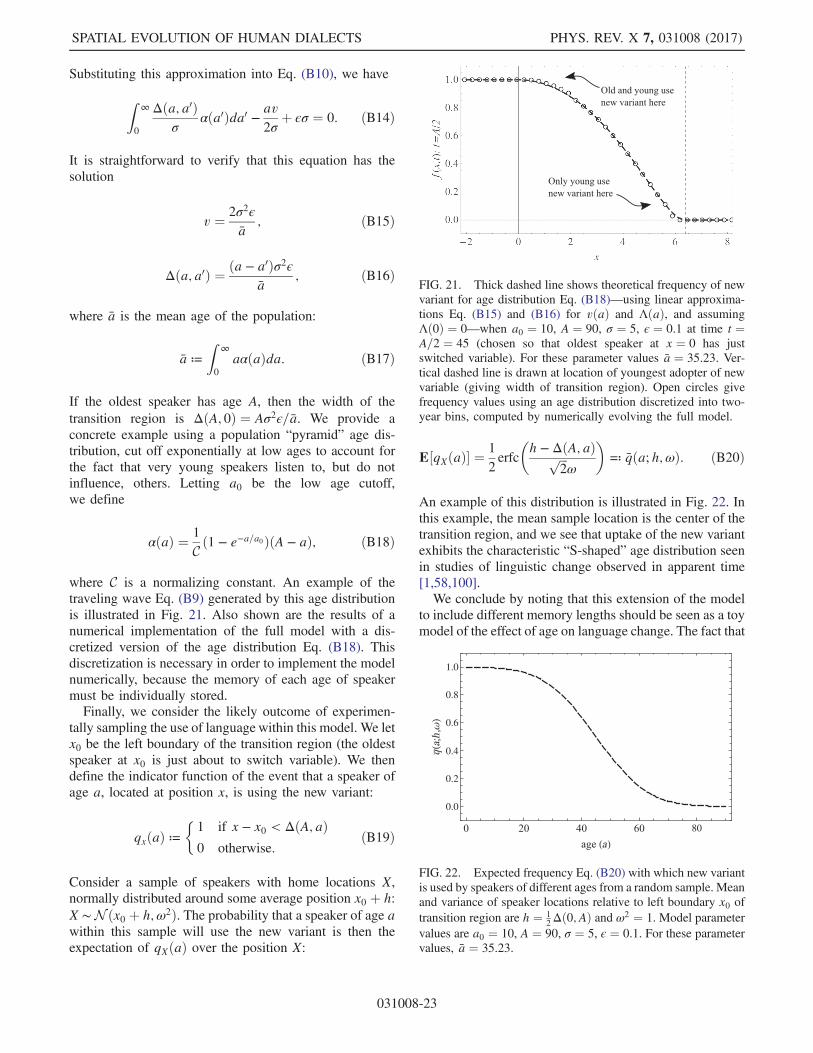
Substituting this approximation into Eq. (B10), we have

Z∞

0

Δða; a0Þσ

αða0Þda0 − av2σ

þ ϵσ ¼ 0: ðB14Þ

It is straightforward to verify that this equation has thesolution

v ¼ 2σ2ϵ

a; ðB15Þ

Δða; a0Þ ¼ ða − a0Þσ2ϵa

; ðB16Þ

where a is the mean age of the population:

a ≔Z

∞

0

aαðaÞda: ðB17Þ

If the oldest speaker has age A, then the width of thetransition region is ΔðA; 0Þ ¼ Aσ2ϵ=a. We provide aconcrete example using a population “pyramid” age dis-tribution, cut off exponentially at low ages to account forthe fact that very young speakers listen to, but do notinfluence, others. Letting a0 be the low age cutoff,we define

αðaÞ ¼ 1

Cð1 − e−a=a0ÞðA − aÞ; ðB18Þ

where C is a normalizing constant. An example of thetraveling wave Eq. (B9) generated by this age distributionis illustrated in Fig. 21. Also shown are the results of anumerical implementation of the full model with a dis-cretized version of the age distribution Eq. (B18). Thisdiscretization is necessary in order to implement the modelnumerically, because the memory of each age of speakermust be individually stored.Finally, we consider the likely outcome of experimen-

tally sampling the use of language within this model. We letx0 be the left boundary of the transition region (the oldestspeaker at x0 is just about to switch variable). We thendefine the indicator function of the event that a speaker ofage a, located at position x, is using the new variant:

qxðaÞ ≔�1 if x − x0 < ΔðA; aÞ0 otherwise:

ðB19Þ

Consider a sample of speakers with home locations X,normally distributed around some average position x0 þ h:X ∼N ðx0 þ h;ω2Þ. The probability that a speaker of age awithin this sample will use the new variant is then theexpectation of qXðaÞ over the position X:

E½qXðaÞ� ¼1

2erfc

�h − ΔðA; aÞffiffiffi

2p

ω

�≕ qða; h;ωÞ: ðB20Þ

An example of this distribution is illustrated in Fig. 22. Inthis example, the mean sample location is the center of thetransition region, and we see that uptake of the new variantexhibits the characteristic “S-shaped” age distribution seenin studies of linguistic change observed in apparent time[1,58,100].We conclude by noting that this extension of the model

to include different memory lengths should be seen as a toymodel of the effect of age on language change. The fact that

FIG. 21. Thick dashed line shows theoretical frequency of newvariant for age distribution Eq. (B18)—using linear approxima-tions Eq. (B15) and (B16) for vðaÞ and ΛðaÞ, and assumingΛð0Þ ¼ 0—when a0 ¼ 10, A ¼ 90, σ ¼ 5, ϵ ¼ 0.1 at time t ¼A=2 ¼ 45 (chosen so that oldest speaker at x ¼ 0 has justswitched variable). For these parameter values a ¼ 35.23. Ver-tical dashed line is drawn at location of youngest adopter of newvariable (giving width of transition region). Open circles givefrequency values using an age distribution discretized into two-year bins, computed by numerically evolving the full model.

0.0

80

0.2

0.4

0.6

0.8

1.0

FIG. 22. Expected frequency Eq. (B20) with which new variantis used by speakers of different ages from a random sample. Meanand variance of speaker locations relative to left boundary x0 oftransition region are h ¼ 1

2Δð0; AÞ and ω2 ¼ 1. Model parameter

values are a0 ¼ 10, A ¼ 90, σ ¼ 5, ϵ ¼ 0.1. For these parametervalues, a ¼ 35.23.


031008-23

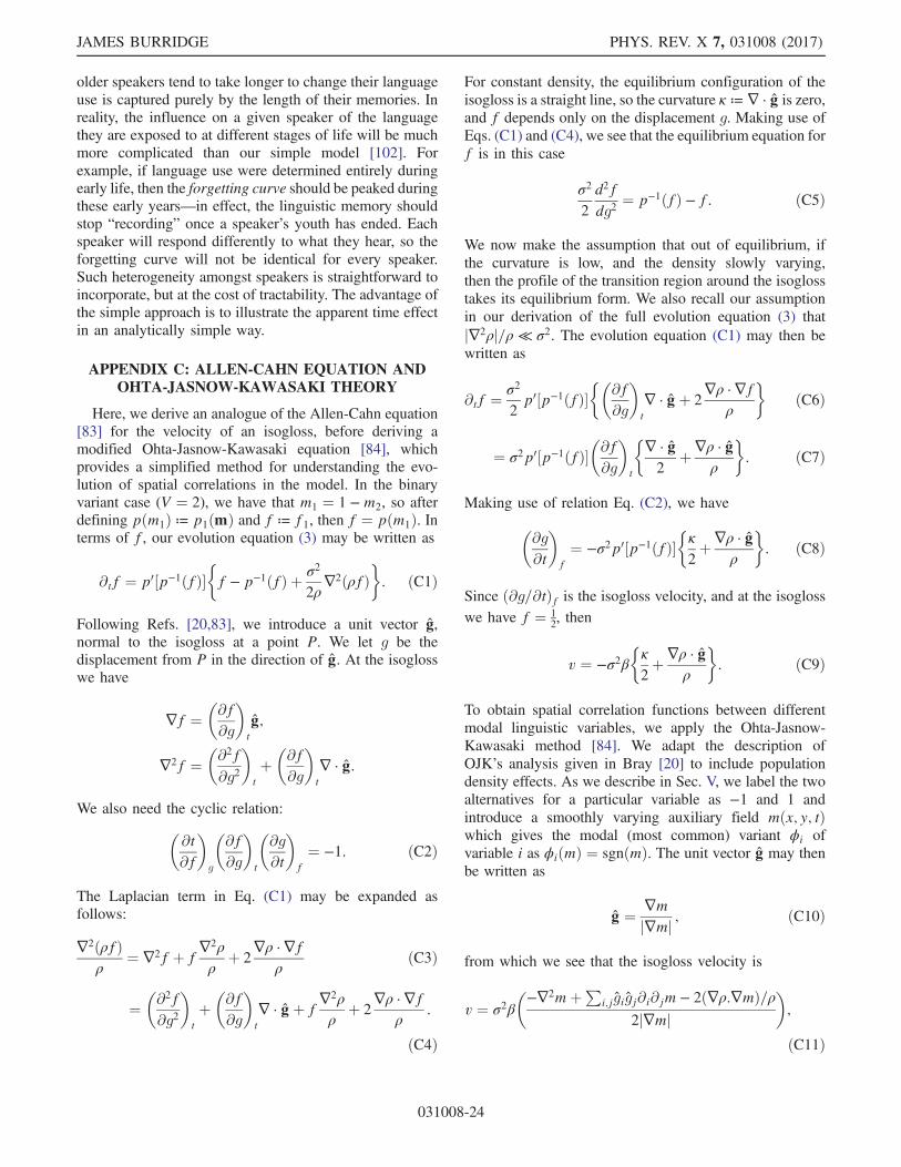
older speakers tend to take longer to change their languageuse is captured purely by the length of their memories. Inreality, the influence on a given speaker of the languagethey are exposed to at different stages of life will be muchmore complicated than our simple model [102]. Forexample, if language use were determined entirely duringearly life, then the forgetting curve should be peaked duringthese early years—in effect, the linguistic memory shouldstop “recording” once a speaker’s youth has ended. Eachspeaker will respond differently to what they hear, so theforgetting curve will not be identical for every speaker.Such heterogeneity amongst speakers is straightforward toincorporate, but at the cost of tractability. The advantage ofthe simple approach is to illustrate the apparent time effectin an analytically simple way.

APPENDIX C: ALLEN-CAHN EQUATION ANDOHTA-JASNOW-KAWASAKI THEORY

Here, we derive an analogue of the Allen-Cahn equation[83] for the velocity of an isogloss, before deriving amodified Ohta-Jasnow-Kawasaki equation [84], whichprovides a simplified method for understanding the evo-lution of spatial correlations in the model. In the binaryvariant case (V ¼ 2), we have that m1 ¼ 1 −m2, so afterdefining pðm1Þ ≔ p1ðmÞ and f ≔ f1, then f ¼ pðm1Þ. Interms of f, our evolution equation (3) may be written as

∂tf ¼ p0½p−1ðfÞ��f − p−1ðfÞ þ σ2

2ρ∇2ðρfÞ

�: ðC1Þ

Following Refs. [20,83], we introduce a unit vector g,normal to the isogloss at a point P. We let g be thedisplacement from P in the direction of g. At the isoglosswe have

∇f ¼�∂f∂g

�tg;

∇2f ¼�∂2f∂g2

�tþ�∂f∂g

�t∇ · g:

We also need the cyclic relation:�∂t∂f

�g

�∂f∂g

�t

�∂g∂t�

f¼ −1: ðC2Þ

The Laplacian term in Eq. (C1) may be expanded asfollows:

∇2ðρfÞρ

¼ ∇2f þ f∇2ρ

ρþ 2

∇ρ ·∇fρ

ðC3Þ

¼�∂2f∂g2

�tþ�∂f∂g

�t∇ · gþ f

∇2ρ

ρþ 2

∇ρ ·∇fρ

:

ðC4Þ

For constant density, the equilibrium configuration of theisogloss is a straight line, so the curvature κ ≔ ∇ · g is zero,and f depends only on the displacement g. Making use ofEqs. (C1) and (C4), we see that the equilibrium equation forf is in this case

σ2

2

d2fdg2

¼ p−1ðfÞ − f: ðC5Þ

We now make the assumption that out of equilibrium, ifthe curvature is low, and the density slowly varying,then the profile of the transition region around the isoglosstakes its equilibrium form. We also recall our assumptionin our derivation of the full evolution equation (3) thatj∇2ρj=ρ ≪ σ2. The evolution equation (C1) may then bewritten as

∂tf ¼ σ2

2p0½p−1ðfÞ�

��∂f∂g

�t∇ · gþ 2

∇ρ · ∇fρ

�ðC6Þ

¼ σ2p0½p−1ðfÞ��∂f∂g

�t

�∇ · g2

þ∇ρ · gρ

�: ðC7Þ

Making use of relation Eq. (C2), we have

�∂g∂t�

f¼ −σ2p0½p−1ðfÞ�

�κ

2þ∇ρ · g

ρ

�: ðC8Þ

Since ð∂g=∂tÞf is the isogloss velocity, and at the isoglosswe have f ¼ 1

2, then

v ¼ −σ2β�κ

2þ∇ρ · g

ρ

�: ðC9Þ

To obtain spatial correlation functions between differentmodal linguistic variables, we apply the Ohta-Jasnow-Kawasaki method [84]. We adapt the description ofOJK’s analysis given in Bray [20] to include populationdensity effects. As we describe in Sec. V, we label the twoalternatives for a particular variable as −1 and 1 andintroduce a smoothly varying auxiliary field mðx; y; tÞwhich gives the modal (most common) variant ϕi ofvariable i as ϕiðmÞ ¼ sgnðmÞ. The unit vector g may thenbe written as

g ¼ ∇mj∇mj ; ðC10Þ

from which we see that the isogloss velocity is

v ¼ σ2β

�−∇2mþPi;jgigj∂i∂jm − 2ð∇ρ:∇mÞ=ρ

2j∇mj�;

ðC11Þ


031008-24

where i; j ∈ fx; yg. In a reference frame attached to theinterface,

dmdt

¼ 0 ¼ ∂m∂t þ v · ∇m: ðC12Þ

Since v∥∇m, then v ·∇m ¼ vj∇mj and ∂tm ¼ −vj∇mj, so

∂m∂t ¼ σ2β

2

�∇2m −

Xi;j

gigj∂i∂jmþ 2∇ρ:∇m

ρ

�: ðC13Þ

This is the OJK equation, modified to include variablepopulation density. As OJK did, we now assume that thedirection g is uniformly distributed over the system, and wereplace gigj with its circular mean 1

2δij, giving

∂m∂t ¼ σ2β

�∇2m4

þ∇ρ:∇mρ

�: ðC14Þ

This is our modified Ohta-Jasnow-Kawasaki equation.

APPENDIX D: COMPARISON WITH ASIMULATION OF NERBONNE

We note a link between curve Eq. (19) and a simplemodel simulated by Nerbonne [39], but not characterizedanalytically. The model consists of a line of discrete spatialpoints, with a single reference site at one end representing acity. In contrast to our model, all sites initially use anidentical set of N (¼ 100 in Ref. [39]) binary linguisticvariables. Evolution of language use is simulated at eachsite by repeatedly selecting a variable at random and thenchanging the state of the variable with probability 1

2. For a

site at distance r from the city, the number of repeats of thisrandomization process is defined as nðrÞ ≔ ⌊Crα⌋, wherethe constant α measures the spatial decline of the “influ-ence” of the city with r. Larger values of nðrÞ imply agreater level of noisy evolution and therefore a lowerinfluence of the city. Linguistic distance in this model,after each site has received its nðrÞ updates, is given by

lðrÞ ¼ 1

2½1 − ð1 − N−1ÞnðrÞ� ≈ 1

2½1 − e−nðrÞ=N�: ðD1Þ

In Ref. [39], two values of α are tested, α ¼ 1, 2, and thequadratic case is identified as being consistent withTrudgill’s macroscopic gravity model. However, weemphasize that the two models do not make predictionsthat can be directly compared: in the microscopic model[39] no indication is given of how two centers of influencewould compete. Of interest is the fact that the α ¼ 2 casecoincides with our prediction for large r. However, thisvalue of α is rejected in Ref. [39] on the basis of itssigmoidal shape for small r. Because of the presence of the

inverse sine function, this behavior is not present in ourversion of Séguy’s law [Eq. (19)]. We note also that thedynamics of Ref. [39] reduce order in the system, whereasour model leads to increasingly ordered states.

[1] J. K. Chambers and P. Trudgill, Dialectology (CambridgeUniversity Press, Cambridge, England, 1998).

[2] W. Heeringa and J. Nerbonne, Dialect Areas and DialectContinua, Lang. Var. Change 13, 375 (2001).

[3] L. Bloomfield, Language (Holt, Rinehart and Winston,New York, 1933).

[4] P. Trudgill, The Dialects of England (Blackwell, Hoboken,NJ, 1999).

[5] J. Séguy, La Relation Entre la Distance Spatiale et laDistance Lexicale, Rev. Ling. Romane 35, 335 (1971).

[6] J. Séguy, La Dialectomtrie Dans l’Atlas Linguistique de laGascogne, Rev. Ling. Romane 37, 1 (1973).

[7] M. Wieling and J. Nerbonne, Advances in Dialectometry,Annu. Rev. Ling. 1, 243 (2015).

[8] B. Kessler, in Proceedings of the 7th Conference of theEuropean Chapter of the Association for ComputationalLinguistics (Morgan Kaufmann Publishers Inc., SanFrancisco, CA, 1995), pp. 60–67.

[9] V. Levenshtein, Binary Codes Capable of CorrectingDeletions, Insertions and Reversals, Dokl. Akad. NaukSSSR 163, 845 (1965).

[10] R. G. Shackelton, Jr., Phonetic Variation in the TraditionalEnglish Dialects. A Computational Analysis, J. Engl. Ling.35, 30 (2007).

[11] S. Embleton, D. Uritescu, and E. S. Wheeler, DefiningDialect Regions with Interpretations: Advancing theMultidimensional Scaling Approach, Literary Ling.Comput. 28, 13 (2013).

[12] M. Wieling and J. Nerbonne, Bipartite Spectral GraphPartitioning for Clustering Dialect Varieties andDetecting Their Linguistic Features, Comput. SpeechLang. 25, 700 (2011).

[13] M. Wieling and J. Nerbonne, GABMAP: A Web Applicationfor Dialectology, Dialectologia II, 65 (2011).

[14] P. Trudgill, Linguistic Change and Diffusion: Descriptionand Explanation in Sociolinguistic Dialect Geography,Lang. Soc. 3, 215 (1974).

[15] W. Wolfram and N. Schilling-Estes, Dialectology andLinguistic Diffusion, in The Handbook of HistoricalLinguistics, edited by B. D. Joseph and R. D. Janda(Blackwell Publishing, Malden, 2003), pp. 713–725.

[16] W. Labov, Social Dialectology in Honour of Peter Trudgill(John Benjamins Publishing Company, Amsterdam,2003), pp. 9–22.

[17] G. Bailey, T. Wikle, J. Tillery, and L. Sand, Some Patternsof Linguistic Diffusion, Lang. Var. Change 5, 359 (1993).

[18] J. N. Stanford and L. A. Kenney, Revisiting Transmissionand Diffusion: An Agent-Based Model of Vowel ChainShifts Across Large Communities, Lang. Var. Change 25,119 (2013).

[19] D. Crystal, The Cambridge Encyclopedia of the EnglishLanguage (Cambridge University Press, Cambridge,England, 2003).


031008-25

https://doi.org/10.1017/S0954394501133041

https://doi.org/10.5169/seals-399508

https://doi.org/10.5169/seals-399527

https://doi.org/10.1146/annurev-linguist-030514-124930

https://doi.org/10.1177/0075424206297857

https://doi.org/10.1177/0075424206297857

https://doi.org/10.1093/llc/fqs048

https://doi.org/10.1093/llc/fqs048

https://doi.org/10.1016/j.csl.2010.05.004

https://doi.org/10.1016/j.csl.2010.05.004

https://doi.org/10.1017/S0047404500004358

https://doi.org/10.1017/S095439450000154X

https://doi.org/10.1017/S0954394513000069

https://doi.org/10.1017/S0954394513000069

[20] A. J. Bray, Theory of Phase-Ordering Kinetics, Adv. Phys.43, 357 (1994).

[21] K. Barros, P. L. Krapivsky, and S. Redner, Freezing intoStripe States in Two-Dimensional Ferromagnets andCrossing Probabilities in Critical Percolation, Phys.Rev. E 80, 040101 (2009).

[22] P. L. Krapivsky, S. Redner, and E. Ben-Naim, A KineticView of Statistical Physics (Cambridge University Press,Cambridge, England, 2010).

[23] J. Burridge and S. Kenney, Birdsong Dialect PatternsExplained Using Magnetic Domains, Phys. Rev. E 93,062402 (2016).

[24] M. Gerlach and E. G. Altmann, Stochastic Model for theVocabulary Growth in Natural Languages, Phys. Rev. X3, 021006 (2013).

[25] A. M. Petersen, J. N. Tenenbaum, S. Havlin, H. E. Stanley,and M. Perc, Languages Cool as They Expand: AllometricScaling and the Decreasing Need for New Words, Sci.Rep. 2, 943 (2012).

[26] J. C. Willis and G. U. Yule, Some Statistics of Evolutionand Geographical Distribution in Plants and Animals, andTheir Signature, Nature (London) 109, 177 (1922).

[27] M. E. J. Newman, Power Laws, Pareto Distributions andZipf’s Law, Contemp. Phys. 46, 323 (2005).

[28] M. Gerlach and E. G. Altmann, Scaling Laws andFluctuations in the Statistics of Word Frequencies,New J. Phys. 16, 113010 (2014).

[29] M. Newman, Networks: An Introduction, (Oxford,New York, 2010).

[30] J. P. Gleeson, K. P. O’Sullivan, R. A. Banos, and Y.Moreno, Effects of Network Structure, Competitionand Memory Time on Social Spreading Phenomena.,Phys. Rev. X 6, 021019 (2016).

[31] R. Albert, H. Jeong, and A. L. Barabasi, Error and AttackTolerance of Complex Networks, Nature (London) 406,378 (2000).

[32] M. Perc, Evolution of the Most Common English Wordsand Phrases Over the Centuries, J. R. Soc. Interface 9,3323 (2012).

[33] V. V. Loreto, A. Baronchelli, A. Mukherjee, A. Puglisi, andF. Tria, Statistical Physics of Language Dynamics, J. Stat.Mech. (2011) P04006.

[34] G. J. Baxter, R. A. Blythe, W. Croft, and A. J. McKane,Utterance Selection Model of Language Change, Phys.Rev. E 73, 046118 (2006).

[35] M. R. D’Orsogna and M. Perc, Statistical Physics ofCrime: A Review, Phys. Life Rev. 12, 1 (2015).

[36] Z. Wanga, C. T. Bauch, Samit Bhattacharyya, A.d’Onofrio, P. Manfredi, M. Perc, N. Perra, M. Salathé,and D. Zhaol, Statistical Physics of Vaccination, Phys.Rep. 664, 1 (2016).

[37] C. Castellano, S. Fortunato, and V. Loreto, StatisticalPhysics of Social Dynamics, Rev. Mod. Phys. 81, 591(2009).

[38] See Supplemental Material at http://link.aps.org/supplemental/10.1103/PhysRevX.7.031008 for animatedversions of Fig. 6, Fig. 10, Fig. 18, and a spreadsheetimplementation of the discretized evolution equationderived in Appendix A.

[39] J. Nerbonne, Measuring the Diffusion of LinguisticChange, Phil. Trans. R. Soc. B 365, 3821 (2010).

[40] M. R. Mehl, S. Vazire, N. Ramrez-Esparza, R. B. Slatcher,and J. W. Pennebaker, Are Women Really More TalkativeThan Men?, Science 317, 82 (2007).

[41] J. K. Chambers, Dialect Acquisition, Language 68, 673(1992).

[42] J. Siegel, SecondDialect Acquisition (Cambridge UniversityPress, Cambridge, England, 2010).

[43] P. Bloom, How Children Learn the Meanings of Words(MIT Press, Cambridge, MA, 2000).

[44] G. Sankoff and H. Blondeau, Language Change Across theLifespan: /r/ in Montreal French, Language 83, 560(2007).

[45] L. Averell and A Heathcote, The Form of the ForgettingCurve and the Fate of Memories, J. Math. Psychol. 55. 25(2011).

[46] R. A. Blythe, Neutral Evolution: A Null Model forLanguage Dynamics, Adv. Complex Syst. 15, 1150015(2012).

[47] J. Mathews and R. L. Walker, Mathematical Methods ofPhysics (Addison-Wesley, Reading, MA, 1971).

[48] W. Croft, Explaining Language Change: An EvolutionaryApproach (Longman, Harlow, England, 2000).

[49] M. Kimura, The Neutral Theory of Molecular Evolu-tion (Cambridge University Press, Cambridge, England,1983).

[50] P. A. P Moran, Random Processes in Genetics, Proc.Cambridge Philos. Soc. 54, 60 (1958).

[51] S. Asch, Studies of Independence and Conformity: I. AMinority of One Against a Unanimous Majority, Psychol.Monogr. 70, 1 (1956).

[52] R. Bond and P. B. Smith, Culture and Conformity: A Meta-Analysis of Studies Using Asch’s (1952b, 1956) LineJudgment Task, Psychol. Bull. 119, 111 (1996).

[53] T. J. H. Morgan, L. E. Rendell, M. Ehn, W. Hoppitt, andK. N. Laland, The Evolutionary Basis of Human SocialLearning, Proc. R. Soc. B 279, 653 (2012).

[54] D. A. Nelson, Song Overproduction, Selective Attritionand Song Dialects in the White-Crowned Sparrow, AnimalBehaviour 60, 887 (2000).

[55] P. Trudgill, Sociolinguistics (Penguin, London, 2000).[56] W. Labov, The Social Stratification of English in New York

City (Cambridge University Press, Cambridge, England,2006).

[57] A. S. Kroch, Toward a Theory of Social Dialect Variation,Lang. Soc. 7, 17 (1978).

[58] W. Labov, Principles of Linguistic Change (Blackwell,Malden, MA, 2001).

[59] W. Labov, The Social Motivation of a Sound Change,Word and Information Processing 19, 273 (1963).

[60] W. Wolfram and N. Schilling-Estes, in SociolinguisticVariation: Data, Theory, and Analysis: Selected Papersfrom NWAV 23 at Stanford (CSLI, Stanford, CA, 1996),pp. 69–82.

[61] W. Labov, Sociolinguistic Patterns (University ofPennsylvania Press, Philadelphia, PA, 1972).

[62] D. MacAulay, The Celtic Languages (Cambridge Univer-sity Press, Cambridge, England, 2008).


031008-26

https://doi.org/10.1080/00018739400101505

https://doi.org/10.1080/00018739400101505

https://doi.org/10.1103/PhysRevE.80.040101






https://doi.org/10.1038/srep00943

https://doi.org/10.1038/srep00943

https://doi.org/10.1038/109177a0

https://doi.org/10.1080/00107510500052444

https://doi.org/10.1088/1367-2630/16/11/113010


https://doi.org/10.1038/35019019

https://doi.org/10.1038/35019019

https://doi.org/10.1098/rsif.2012.0491

https://doi.org/10.1098/rsif.2012.0491

https://doi.org/10.1088/1742-5468/2011/04/P04006

https://doi.org/10.1088/1742-5468/2011/04/P04006



https://doi.org/10.1016/j.plrev.2014.11.001

https://doi.org/10.1016/j.physrep.2016.10.006

https://doi.org/10.1016/j.physrep.2016.10.006

https://doi.org/10.1103/RevModPhys.81.591

https://doi.org/10.1103/RevModPhys.81.591

http://link.aps.org/supplemental/10.1103/PhysRevX.7.031008







https://doi.org/10.1098/rstb.2010.0048

https://doi.org/10.1126/science.1139940

https://doi.org/10.1353/lan.1992.0060

https://doi.org/10.1353/lan.1992.0060

https://doi.org/10.1353/lan.2007.0106

https://doi.org/10.1353/lan.2007.0106

https://doi.org/10.1016/j.jmp.2010.08.009

https://doi.org/10.1016/j.jmp.2010.08.009

https://doi.org/10.1142/S0219525911003414

https://doi.org/10.1142/S0219525911003414

https://doi.org/10.1017/S0305004100033193

https://doi.org/10.1017/S0305004100033193

https://doi.org/10.1037/h0093718

https://doi.org/10.1037/h0093718

https://doi.org/10.1037/0033-2909.119.1.111

https://doi.org/10.1098/rspb.2011.1172

https://doi.org/10.1006/anbe.2000.1560

https://doi.org/10.1006/anbe.2000.1560

https://doi.org/10.1017/S0047404500005315

https://doi.org/10.1080/00437956.1963.11659799

[63] W. H. Press, S. A. Teukolsky, W. T. Vetterling, and B. P.Flannery, Numerical Recipes (Cambridge University Press,Cambridge, England, 2007).

[64] Office for National Statistics: 2011 Census aggregate data,UK Data Service, 2016, http://dx.doi.org/10.5257/census/aggregate‑2011‑1.

[65] M. Tranter, D. Robineau, and G. Goodman, NationalTravel Survey: 2014 Report (Department of Transport,United Kingdom, 2014), https://www.gov.uk/government/statistics/national‑travel‑survey‑2014.

[66] P.-G. de Gennes, F. Brochard-Wyart, and D. Quere,Capillarity and Wetting Phenomena (Springer-Verlag,New York, 2004).

[67] C. Upton, The Importance of Being Janus: MidlandSpeakers and the “North-South Divide”, in Middle andModern English Corpus Linguistics, edited by M. Markus,Y. Iyeiri, R. Heuberger, and E. Chamson (John BenjaminsPublishing Company, Amsterdam, 2012), pp. 257–268.

[68] W. J. Heeringa, Measuring Dialect PronunciationDifferences Using Levenshtein Distance (University ofGroningen, Groningen, 2004).

[69] A. K. Jain and R. C. Dubes, Algorithms for ClusteringData (Prentice-Hall, Englewood Cliffs, NJ, 1988.

[70] M. Maechler, P. Rousseeuw, A. Struyf, M. Hubert, andK. Hornik, Cluster: Cluster Analysis Basics and Exten-sions. 2016. R package version 2.0.5. For new features,see the “Changelog” file (in the package source), https://cran.r‑project.org/web/packages/cluster.

[71] B Everitt, S. Landau, M. Leese, and D. Stahl, ClusterAnalysis (Wiley, Chichester, England, 2011).

[72] H Kuhn, The Hungarian Method for the AssignmentProblem, Naval research logistics quarterly 2, 83 (1955).

[73] S. N. Chiu, D. Stoyan, W. Kendall, and J. Mecke, Sto-chastic Geometry and Its Applications (Wiley, Chichester,England, 2013).

[74] W.M. Rand, Objective Criteria for the Evaluation ofClustering Methods, J. Am. Stat. Assoc. 66, 846 (1971).

[75] L. Hubert, Comparing Partitions, J. Classif. 2, 193(1985).

[76] W. Heeringa, J. Nerbonne, and P. Kleiweg, ValidatingDialect Comparison Methods, in Classification, Automa-tion, and New Media (Springer-Verlag, Berlin, 2002),pp. 445–452.

[77] P. Sammallahti, The Saami Languages. An Introduction(Dawi Girji, Karasjok, Norway, 1998).

[78] D. R. Preston,Handbook of Perceptual Dialectology (JohnBenjamins, Amsterdam, 1999).

[79] M. R. Spruit, W. Heeringa, and J. Nerbonne, Associationsamong Linguistic Levels, Lingua 119, 1624 (2009).

[80] C. Gooskens, Traveling Time as a Predictor of LinguisticDistance, Dialectologia Geolinguistica 13, 38 (2005).

[81] S. Montemagni, The Space of Tuscan Dialectal Variation.A Correlation Study, Int. J. Humanit. Arts Comput. 2, 135(2008).

[82] J. Nerbonne and P. Kleiweg, Lexical Distance in Lamsas,Comput. Humanit. 37, 339 (2003).

[83] S. M. Allen and J. W. Cahn, A Microscopic Theoryfor Antiphase Boundary Motion and Its Application toAntiphase Domain Coarsening, Acta Metall. 27, 1085(1979).

[84] T. Ohta, D. Jasnow, and K. Kawasaki, Universal Scaling inthe Motions of Random Interfaces, Phys. Rev. Lett. 49,1223 (1982).

[85] Y. Oono and S. Puri, Large Wave Number Features ofForm Factors for Phase Transition Kinetics, Mod. Phys.Lett. B 02, 861 (1988).

[86] S. V. Patankar, Numerical Heat Transfer and Fluid Flow(McGraw-Hill, New York, 1980).

[87] T. Leinonen, An Acoustic Analysis of Vowel Pronunciationin Swedish Dialects (Rijksuniversiteit Groningen, 2010).

[88] David Morin, Introduction to Classical Mechanics(Cambridge University Press, Cambridge, England, 2008).

[89] NIST Handbook of Mathematical Functions, edited byF.W. J. Olver, D. W. Lozier, R. F. Boisvert, and C.W.Clark (Cambridge University Press, Cambridge, England,2010).

[90] D. Brockmann, L. Hufnagel, and T. Geisel, The ScalingLaws of Human Travel, Nature (London) 439, 462 (2006).

[91] M. C. Gonzlez, C. A. Hidalgo, and L. A. Barabsi, Under-standing Individual Human Mobility Patterns, Nature(London) 453, 779 (2008).

[92] H. Hayakawa, T Ishihara, K. Kawanishi, and T. S.Kobayakawa, Phase-Ordering Kinetics in NonconservedScalar Systems with Long-Range Interactions, Phys. Rev.E 48, 4257 (1993).

[93] T. Blanchard, M. Picco, and M. A. Rajabpour, Influence ofLong-Range Interactions on the Critical Behavior of theIsing Model, Europhys. Lett. 101, 56003 (2013).

[94] B. D. Joseph and R. D. Janda, The Handbook of HistoricalLinguistics (Blackwell, Oxford, 2003).

[95] C.-M. Pop and E. Frey, Language Change in a MultipleGroup Society, Phys. Rev. E 88, 022814 (2013).

[96] P. Roach, English Phonetics and Phonology (CambridgeUniversity Press, Cambridge, England, 2009).

[97] M. Davenport and S. J. Hannahs, Introducing Phoneticsand Phonology (Routledge, Oxford, 2010).

[98] Leo Tolstoy, War and Peace (Penguin, Toronto, 1869).[99] P. M. B. Vitányi, Tolstoy’s Mathematics in War and Peace,

Math. Intelligence 35, 71 (2013).[100] J. K. Chambers, The Canada US Border as a Vanishing

Isogloss: The Evidence of Chesterfield, J. Engl. Ling. 23,155 (1995).

[101] G. Bailey, T. Wilke, J. Tillery, and L. Sand, The ApparentTime Construct, Lang. Var. Change 3, 241 (1991).

[102] G. Baxter and W. Croft, Modeling Language ChangeAcross the Lifespan: Individual Trajectories in CommunityChange, Lang. Var. Change 28, 129 (2016).


031008-27

http://dx.doi.org/10.5257/census/aggregate-2011-1





https://www.gov.uk/government/statistics/national-travel-survey-2014




https://cran.r-project.org/web/packages/cluster




https://doi.org/10.1002/nav.3800020109

https://doi.org/10.1080/01621459.1971.10482356

https://doi.org/10.1007/BF01908075

https://doi.org/10.1007/BF01908075

https://doi.org/10.1016/j.lingua.2009.02.001

https://doi.org/10.1515/dig.2005.2005.13.38

https://doi.org/10.3366/E1753854809000354

https://doi.org/10.3366/E1753854809000354

https://doi.org/10.1023/A:1025042402655

https://doi.org/10.1016/0001-6160(79)90196-2

https://doi.org/10.1016/0001-6160(79)90196-2

https://doi.org/10.1103/PhysRevLett.49.1223

https://doi.org/10.1103/PhysRevLett.49.1223

https://doi.org/10.1142/S0217984988000606

https://doi.org/10.1142/S0217984988000606

https://doi.org/10.1038/nature04292





https://doi.org/10.1209/0295-5075/101/56003


https://doi.org/10.1007/s00283-012-9342-8

https://doi.org/10.1177/0075424290023001-213

https://doi.org/10.1177/0075424290023001-213

https://doi.org/10.1017/S0954394500000569

https://doi.org/10.1017/S0954394516000077

Spatial Evolution of Human Dialects - Physics

Documents

Transcript of Spatial Evolution of Human Dialects - Physics