Spatial Error Analysis of Species Richness for a Gap Analysis Map

Denis J. Dean, Kenneth R. Wilson, and Curtis H. Rather

Abstract Variation in the distribution of species richness as a result of introduced errors of omission and commission in the Gap Analysis database for Oregon was evaluated using Monte Carlo simulations. Random errors, assumed to be indepen-dent of a species' distribution, and boundary errors, assumed to be dependent on the species' distribution, were simulated using ten rodent species. Error rates of omission and com-mission equal to 5 and 20 percent were used in the simula-tions. Indications are that predictions of species richness within a Gap Analysis database can be very sensitive to both types of errors with sensitivity to random error being much greater. Implications are that the inclusion of error modeling in applied GIS databases is critical to spatially explicit con-servation recommendations.

Introduction With increasing use of remote sensing and geographic infor-mation system (GIS) databases, the concern with accuracy and how to assess accuracy has grown (Goodchild and Go-pal, 1989; Story and Congalton, 1986; Jansen and van der Wel, 1994). Sources of error include lack of spatial and the-matic accuracy (Janssen and van der Wel, 1994), but lineage of the data and temporal accuracy can also be important (Thapa and Bossler, 1992; Lanter and Veregin, 1992). There is also a need to understand how error propagation can affect the results of a layer-based GIS (Veregin, 1989; Lanter and Veregin, 1992; Veregin, 1994).

The Gap Analysis Project (GAP), which utilizes a layer-based GIS, has emerged as a strategy for conserving biological diversity (Scott et al., 1987; Scott et al., 1993). GAP studies have been conducted on a state-by-state basis, and specific guidelines for conducting GAP studies are outlined in Ma and Redmond (1992), Scott et al. (1993), Jennings (1993), and USDI, National Biological Survey (1994). In general, the ba-sic steps in a Gap Analysis are (1) the development of a vege-tation map based on Landsat Thematic Mapper (TM) imagery and other information, (2) the development of a species dis-tribution map based on existing range maps and other dis-tributional data as well as the use of habitat-relationship models (see Morrison et al., 1992), and (3) combining these maps to identify habitats and species that are underrepre-sented in the current network of biodiversity management ar-eas. One parameter of interest in a Gap Analysis is a map of species richness which is then combined with additional map layers containing land-management and ownership in-

D.J. Dean is with the Department of Forest Sciences and K.R. Wilson is with the Department of Fishery and Wildlife Biol-ogy, both at Colorado State University, Fort Collins, CO 80523.

C.H. Flather is with the Rocky Mountain Forest and Range Experiment Station, USDA Forest Service, Fort Collins, CO 80523.

formation to identify "gaps" in the protection of species-rich areas, i.e., identify regions of high species richness (biodi-versity) that are not currently within protected areas (see Scott et al., 1993).

The most common procedures used in Gap Analyses to predict species occurrence are based on the intersection of coarse species range information as reflected in vegetation association and county-of-occurrence data (Scott et al., 1993; Butterfield et al., 1994). As such, the habitat selection prob-lem is simplified in only being concerned with predicting species presence/absence. Although simpler, defining and characterizing the geographical range of a species is contro-versial and very imprecise (Rapoport, 1982).

Given these procedures, GAP studies require reasonably accurate habitat-type maps and sound habitat-relationship models. Unfortunately, there has been little work on quanti-fying the sensitivity of GAP results to errors associated with these basic components. It is widely recognized that sensitiv-ity analyses and validation of habitat-based predictions of species occurrence are necessary to evaluate model perform-ance (Lyon et al., 1987; Scott et al., 1993), yet few species-habitat relationship databases have been evaluated (Berry, 1986). Stoms (1992) has examined the sensitivity of GAP studies to the effects of habitat-type map generalization by varying minimum mapping units, but additional study aimed at exploring how habitat-type errors impact GAP results re-mains to be done. Investigations of habitat-relationship mod-els sometimes cast serious doubt on their reliability, which raises concerns regarding the performance of these models in GAP studies. For example, a sensitivity analysis of a habitat-relationship model for the California condor (Gymnogyps cal-ifomianus) indicated that the model was relatively robust to uncertainties in input data (Stoms et al., 1992). But Block et al. (1994) tested habitat-relationship models for relatively well studied taxa such as amphibians, reptiles, birds, and small mammals in California and found that agreement be-tween predictions and residency status ranged from 48 to 78 percent for two databases, with errors of omission (species were not predicted but in fact were observed) and commis-sion (species were predicted but were not observed) ranging from 6 to 39 percent and 20 to 44 percent, respectively.

It is inconceivable that either absolutely error-free habi-tat-type maps or perfect habitat-relationship models can be produced. Thus, GAP studies must incorporate some error from these sources. How these errors affect GAP results and interpretation of these results has not been thoroughly ex-plored.

The objective of this study was to investigate how uncer-

Photogrammetric Engineering & Remote Sensing, Vol. 63, No. 10, October 1997, pp. 1211-1217.

0099-1112/97/6310-1211$3.00/0 0 1997 American Society for Photogrammetry

and Remote Sensing

PE&RS October 1997 1211

Figure 1. Three physiographic regions of Oregon used in the simulations (Puchy and Marshall, 1993). Areas with a species richness 5 are illustrated in black.

tainty in vertebrate species distributions would affect results of a contemporary GAP study. Specifically, we investigated how spatially independent errors and spatially dependent er-rors in species distribution would affect the distribution of species richness as measured by area. Note that no attempt was made to identify the cause of these errors. This study simply investigated results of errors likely to exist in many Gap Analysis projects, regardless of source.

Methods The Oregon GAP GIS database was used in this study (T. O'Neill, pers. comm., Oregon Department of Fish and Wild-life). The Oregon data consisted of a digital vegetation map that divided the state into over 12,000 vegetation polygons based on vegetation cover types (which were identified using satellite imagery), physiographic provinces (based on Puchy and Marshall (1993)), and political boundaries. The Oregon data also included habitat-relationship information for over 800 wildlife species that classified species occurrence based on vegetation type, physiographic region, and political subdi-vision data layers. By combining these digital layers, it was possible to construct a species distribution layer showing the presence or absence of each species in each vegetation poly-gon. Presence or absence data was then used to generate a map of vertebrate species richness.

The fundamental parameter manipulated in this study was the presence or absence of a particular species in a par-ticular polygon based on vegetation/physiographic region/po-litical subdivision. Four possible outcomes are possible from an accuracy assessment. If a species is actually present in a polygon and the GAP procedure predicts species presence, then no error occurs. Similarly, if a species is not present in a polygon and the procedure predicts species absence, then no error occurs. However, if a species is actually present in a polygon but the procedure indicates species absence, then an error of omission occurs. An error of commission occurs if, in fact, a species is not present in a polygon, but the proce-dure indicates species presence.

To evaluate the effect of errors of omission and commis-sion on a GAP study, data received from the Oregon Depart-ment of Fish and Wildlife were considered "truth," i.e., errors were introduced into the Oregon database and esti-mated effects of these introduced errors were compared to the original Oregon GAP database. The independent variable was the level of uncertainty (errors of omission and commis-sion) and the dependent variable was the distribution of spe-cies richness measured as total area in km'.

Monte Carlo computer simulation was used to simulate effects of error on vertebrate species distribution maps using ARC/Info and simulation routines written in C. Each iteration of the Monte Carlo simulation randomly introduced a prede-fined amount of error into the species distribution map, thereby producing a new error-filled species distribution map. Areas of vertebrate species richness in the error-filled map were then compared to areas of vertebrate species rich-ness in the original map in order to quantify changes in the distribution of species richness as a function of the intro-duced errors. Two different techniques were used to intro-duce error into the species distribution map. The first technique introduced spatially independent errors (random errors) throughout the vegetation map without regard to the range of any particular wildlife species. Thus, any polygon in the habitat map where species X did occur was a candi-date for an error of omission of species X and any polygon where species X did not occur was a candidate for an error of commission of species X. An example of these types of er-rors are inaccuracies of vegetation mapping — errors in such maps are unlikely to be dependent upon ranges of the wild-life species found in the mapped region.

The second technique introduced spatially dependent er-rors (boundary errors) along edges of each species "true" range, where the true range was assumed to be the species' range as determined by the original Oregon data. Thus, spa-tially dependent errors only occurred along boundaries of the species' range, with errors of omission occurring in polygons within the true range of the species and errors of commis-sion occurring in polygons just outside the true range. Errors of this sort are likely to occur in GAP studies if inaccuracies in species predictions from habitat-relationship models occur at the boundary of a species range, or if there is difficulty as-sociated with precisely defining boundaries of vegetation polygons.

Total area for each level of species richness was evalu-ated for boundary and random error at simulated error rates of 5 percent and 20 percent. These rates were within the range found in other studies (cf. Flather et al., 1997). For both random and boundary errors, we evaluated the hypoth-esis: Ho: Errors of omission and commission of 5 percent and 20

percent introduce no change in the distribution and amount of total area of vertebrate species richness pres-ent in the results of the Oregon GAP.

We focused on "biological" significance rather than "statisti-cal" significance (e.g., using Student's T-test), because statis-tical significance could have been attained by merely increasing the number of iterations for each simulation.

The Monte Carlo simulations were extremely time con-suming and required large amounts of computer storage space; therefore, we subsetted the original data as follows. A smaller vegetation map was extracted from the original data and a subset of the 800 available species was chosen for analysis. The smaller map consisted of three of the 12 physi-ographic provinces (East Slope Cascades, Basin and Range, and Owyhee Uplands) from the original map and contained 3,238 vegetation polygons (Figure 1). We chose a taxonomi-cally similar subset of the 800 available species. The selected species subset consisted of ten rodents: mountain beaver (Aplodontia rufa), deer mouse (Peromyscus maniculatus), yellow-pine chipmunk (Tamias amoenus), white-tailed ante-lope squirrel (Ammospermophilus leucurus), northern flying squirrel (Glaucomys sabrinus), California kangaroo rat (Dipo-domys califomicus), desert woodrat (Neotoma lepida), heather vole (Phenacomys intermedius), water vole ( Micotus richardsoni), and sagebrush vole (Lemmiscus curtatus). The reduced data sets were joined to create a digital map show-

1212 October 1997 PE&RS

• Original M ap

III 5% Random Error 20% Random Error

ecrs 5 50000

as 40000

30000

WI 20000

10000

0 1 2 3 4 5 6 7

Species Richness Figure 2. Average total area in km2 for polygons with species richness of 0 to 7 for the 50 repeti-tions when random errors were simulated.

ing the distributions of each of the ten rodents throughout the study region, which then became the basis for the Monte Carlo simulations (Figure 1). The original base map for the three physiographic regions included approximately 89,195 km2. Approximately 82,904 km2 (93 percent) of the base map had species richness of 0 to 4 and 6,291 km2 (7 percent) had species richness of 5 or 6. No polygons had a species rich-ness 7 for the original map. Subsets chosen were arbitrary, and implications of the choice of regions and species are ad-dressed in the discussion section.

Each iteration of the Monte Carlo simulation introduced a predefined level of either random or boundary error into the original Oregon data map. Error amounts were measured as percentages. A 5 percent commission error for species X meant that each polygon where species X did not occur had a 5 percent chance of having species X introduced. A 5 percent omission error for species X meant that each polygon where species X occurred had a 5 percent chance of having species X removed. Errors of commission and omission were simulta-neously simulated at the chosen error level. For both random and boundary error, the simulation methods were identical except that, in the boundary-error simulations, errors could only occur in appropriate regions along edges of the various species ranges, whereas random errors could take place any-where within the study area. Appropriate regions for bound-ary error of omission for species X were identified by finding the total area comprising the species' range and symmetri-cally contracting the boundary of the area until 90 percent of the original area remained. The region between the original boundary and the 90 percent contracted-area boundary were deemed to be suitable for errors of omission. Appropriate regions for boundary errors of commission were then identi-fied by expanding the original species X range boundary by the same amount as it was decreased in the previous step and deeming the region between the original and expanded boundaries the appropriate region for commission errors.

The two error rates were used for both random and boundary error cases, resulting in a total of four Monte Carlo simulations. Each simulation consisted of 50 iterations, and each iteration produced a map with species richness for each polygon. The total area by species richness class (i.e., 0, 1, ..., 10 species) was recorded for each iteration. These results were then compared to the results for the original Oregon GAP database. Identification of areas of high species richness (hot spots) is one of the goals of GAP, but rather than arbitrar-ily defining some level of species richness as "hot" (e.g., polygons with more than five species), we present results based on changes in the amount of area for each species richness class. In the case of random error, where expected values for changes in area can be calculated, error matrices (Story and Congalton, 1986) are used to illustrate the results.

Results

Random Error When random error was simulated, areas of species richness changed substantially when compared to the original map (Figure 2). With a 5 percent random error, total area de-creased for species richness of 0, 1, and 4 by an average of 21 to 30 percent and increased for species richness of 2, 3, 5, and 6 by an average of 35 to 158 percent. With a 20 percent random error, the same species richness categories decreased and increased in area, but the effects were magnified with decreases ranging from 50 to 72 percent and increases rang-ing from 57 to 506 percent. For both error rates, there was an increase in total average area for species richness of 7 from 0 km2 in the original data to 292 km2 and 2878 km2 for 5 per-cent and 20 percent error, respectively.

Based on the original species richness categories and a

simulated 5 percent error of omission and commission for each category, an error matrix, using the expected values for the binomial distribution, can be calculated (Table 1). Simu-lated and expected results based on area of species richness were very similar, as can be seen by comparing the Expected Row Total and Simulated Results. Overall theoretical map accuracy was 63 percent and errors of omission range from 35 to 40 percent while errors of commission range from 12 to 76 percent. The high variability in errors of commission are largely dependent on the area size of the nearest species rich category. For example, commission error for species richness of 3 was 63 percent. This result is largely due to the fact that species richness equal to 4 in the original map cov-ered 45,667 km2; consequently, a larger portion, 5,901 km2 , was converted to a species richness of 3 after the simula-tions. The expected error matrix when a 20 percent error of omission and commission is simulated had an overall map accuracy of only 28 percent with errors of omission ranging from 40 to 83 percent and errors of commission ranging from 23 to 95 percent (Table 2).

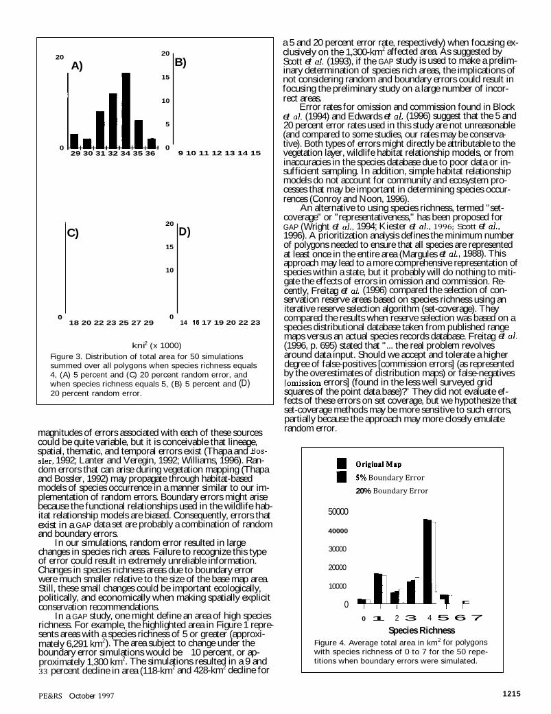
Figure 3 illustrates how the total area with a species richness of 4 and 5 varies for the 50 repetitions of the ran-dom error simulations (a species richness of 4 and 5 were chosen arbitrarily for purposes of illustration, and variability in distributions were similar for other species richness cate-gories). Coefficient of variation of the total average area for species richness of 4 was 5.7 percent and 10.1 percent for random error of 5 and 20 percent, respectively. Coefficient of variation of the total average area for species richness of 5 was 13.8 percent and 12.3 percent for random error of 5 and 20 percent, respectively.

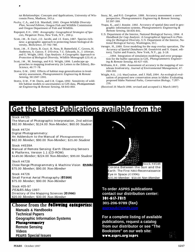
Boundary Error For boundary error simulations, average areas of species richness changed little when compared to the change due to random error (Figure 2 versus Figure 4). Total area decreased on average for a species richness of 0, 1, 4, 5, and 6 by 1 to 21 percent and increased on average for species richness of 2 and 3 by 5 and 8 percent when a 5 percent spatial error was simulated. With a 20 percent boundary error, the same spe-

PE&RS October 1997 1213

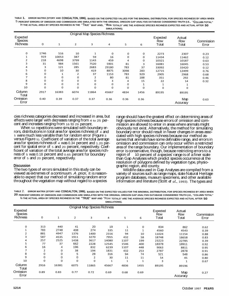
TABLE 1. ERROR MATRIX (STORY AND CONGALTON, 1986), BASED ON THE EXPECTED VALUES FOR THE BINOMIAL DISTRIBUTION, FOR SPECIES RICHNESS BY AREA WHEN 5 PERCENT ERRORS OF OMISSION AND COMMISSION ARE SIMULATED WITH THE ORIGINAL OREGON GAP ANALYSIS DATABASE CONSIDERED TRUTH (I.E., "COLUMN TOTAL"

IS THE ACTUAL AREA BY SPECIES RICHNESS IN THE "TRUE" MAP AND, "Row TOTALS" ARE THE AVERAGE SPECIES RICHNESS EXPECTED AND ACTUAL AFTER 50 SIMULATIONS).

Expected Species

Richness 0 1

Original Map Species Richness

2 3 4 5 6

Expected Row Total

Actual Row Total

Commission Error

0 1746 516 10 1 0 0 0 2273 2307 0.23 1 919 10053 387 59 16 0 0 11434 11462 0.12 2 218 4698 3799 1143 459 4 0 10321 10187 0.63 3 31 984 1561 7520 5901 81 3 16081 16045 0.53 4 3 121 285 2683 29180 783 37 33092 33420 0.12 5 0 10 30 419 8875 3098 283 12715 12499 0.76 6 0 1 2 37 1153 783 929 2905 2968 0.68 7 0 0 0 2 80 81 188 351 292 0.46 8 0 0 0 0 3 4 15 22 14 0.32 9 0 0 0 0 0 0 1 1 1

10 0 0 0 0 0 0 0 0 0

Column 2917 16383 6074 11864 45667 4834 1456 89195 89195 Total

Omission 0.40 0.39 0.37 0.37 0.36 0.36 0.36 Map 0.63 Error Accuracy

cies richness categories decreased and increased in area, but effects were larger with decreases ranging from 4 to 25 per-cent and increases ranging from 16 to 29 percent.

When 50 repetitions were simulated with boundary er-rors, distributions in total area for species richness of 4 and 5 were much less variable than for random error (Figure 3 versus Figure 5). Coefficient of variation of the total average area for species richness of 4 was 0.34 percent and 1.20 per-cent for spatial error of 5 and 20 percent, respectively. Coef-ficient of variation of the total average area for species rich-ness of 5 was 0.18 percent and 0.65 percent for boundary error of 5 and 20 percent, respectively.

Discussion The two types of errors simulated in this study can be viewed as extremes of a continuum. A priori, it is reason-able to expect that our method of simulating random error throughout the vegetation map without regard to a species

range should have the greatest effect on determining areas of high species richness because errors of omission and com-mission are allowed to enter in areas where animals might obviously not exist. Alternatively, the method for simulating boundary error should result in fewer changes in areas asso-ciated with high species richness because our method as-sumes that animals have some definable range, and errors in omission and commission can only occur within a restricted area of the range boundary. Our implementation of boundary error is conservative, though, because restricting errors to a region of ±10 percent of a species' range is of a finer scale than Gap Analyses which predict species occurrence at the resolution of polygons defined by vegetation type, physio-graphic region, and county.

Wildlife data used in Gap Analyses are compiled from a variety of sources such as range maps, state Natural Heritage program databases, museum specimens, and other available information and literature (Scott et al., 1993). The types and

TABLE 2. ERROR MATRIX (STORY AND CONGALTON, 1986), BASED ON THE EXPECTED VALUES FOR THE BINOMIAL DISTRIBUTION, FOR SPECIES RICHNESS BY AREA WHEN 20 PERCENT ERRORS OF OMISSION AND COMMISSION ARE SIMULATED WITH THE ORIGINAL OREGON GAP ANALYSIS DATABASE CONSIDERED TRUTH (I.E., "COLUMN TOTAL"

IS THE ACTUAL AREA BY SPECIES RICHNESS IN THE ''TRUE" MAP AND "Row TOTALS" ARE THE AVERAGE SPECIES RICHNESS EXPECTED AND ACTUAL AFTER 50 SIMULATIONS).

Expected Species

Richness 0 1

Original Map Species Richness

2 3 4 5 6

Expected Row Total

Actual Row Total

Commission Error

0 313 440 41 20 19 1 0 834 862 0.62 1 783 2748 408 274 335 11 1 4560 4543 0.39 2 881 4947 1376 1400 2316 94 10 11024 11154 0.88 3 587 4535 1911 3270 7955 432 58 18748 18658 0.83 4 257 2525 1438 3617 14080 1107 199 23223 22785 0.39 5 77 37 662 2228 12545 1546 400 18378 18911 0.92 6 16 4 196 832 6239 1107 448 9063 8811 0.95 7 2 0 38 194 1831 432 253 2787 2878 0.91 8 0 0 5 28 316 94 74 521 548 0.86 9 0 0 0 2 30 11 11 54 45 0.80

10 0 0 0 0 1 1 1 3 1 0.67

Column 2916 16381 6075 11865 45667 4836 1455 89195 89196 Total

Omission 0.89 0.83 0.77 0.72 0.69 0.68 0.69 Map 0.27 Error Accuracy

1214 October 1997 PE&RS

20 A)

20 B)

15

10

5

0 29 30 31 32 34 35 36 9 10 11 12 13 14 15

20

15

10

C) D)

0 0 18 20 22 23 25 27 29 14 16 17 19 20 22 23

kni2 (x 1000) Figure 3. Distribution of total area for 50 simulations summed over all polygons when species richness equals 4, (A) 5 percent and (C) 20 percent random error, and when species richness equals 5, (B) 5 percent and (D) 20 percent random error.

0

• Original Map

II 5% Boundary Error 20% Boundary Error

Species Richness Figure 4. Average total area in km2 for polygons with species richness of 0 to 7 for the 50 repe-titions when boundary errors were simulated.

0 1 2 3

50000 —

40000 —

30000 —

20000 —

10000 —

0 11!1 Ilmn 4 5 6 7

magnitudes of errors associated with each of these sources could be quite variable, but it is conceivable that lineage, spatial, thematic, and temporal errors exist (Thapa and Bos-sier, 1992; Lanter and Veregin, 1992; Williams, 1996). Ran-dom errors that can arise during vegetation mapping (Thapa and Bossler, 1992) may propagate through habitat-based models of species occurrence in a manner similar to our im-plementation of random errors. Boundary errors might arise because the functional relationships used in the wildlife hab-itat relationship models are biased. Consequently, errors that exist in a GAP data set are probably a combination of random and boundary errors.

In our simulations, random error resulted in large changes in species rich areas. Failure to recognize this type of error could result in extremely unreliable information. Changes in species richness areas due to boundary error were much smaller relative to the size of the base map area. Still, these small changes could be important ecologically, politically, and economically when making spatially explicit conservation recommendations.

In a GAP study, one might define an area of high species richness. For example, the highlighted area in Figure 1 repre-sents areas with a species richness of 5 or greater (approxi-mately 6,291 km2). The area subject to change under the boundary error simulations would be ±10 percent, or ap-proximately 1,300 km2. The simulations resulted in a 9 and 33 percent decline in area (118-km2 and 428-km2 decline for

a 5 and 20 percent error rate, respectively) when focusing ex-clusively on the 1,300-km2 affected area. As suggested by Scott et al. (1993), if the GAP study is used to make a prelim-inary determination of species rich areas, the implications of not considering random and boundary errors could result in focusing the preliminary study on a large number of incor-rect areas.

Error rates for omission and commission found in Block et al. (1994) and Edwards et al. (1996) suggest that the 5 and 20 percent error rates used in this study are not unreasonable (and compared to some studies, our rates may be conserva-tive). Both types of errors might directly be attributable to the vegetation layer, wildlife habitat relationship models, or from inaccuracies in the species database due to poor data or in-sufficient sampling. In addition, simple habitat relationship models do not account for community and ecosystem pro-cesses that may be important in determining species occur-rences (Conroy and Noon, 1996).

An alternative to using species richness, termed "set-coverage" or "representativeness," has been proposed for GAP (Wright et al., 1994; Kiester et al., 1996; Scott et al., 1996). A prioritization analysis defines the minimum number of polygons needed to ensure that all species are represented at least once in the entire area (Margules et al., 1988). This approach may lead to a more comprehensive representation of species within a state, but it probably will do nothing to miti-gate the effects of errors in omission and commission. Re-cently, Freitag et al. (1996) compared the selection of con-servation reserve areas based on species richness using an iterative reserve selection algorithm (set-coverage). They compared the results when reserve selection was based on a species distributional database taken from published range maps versus an actual species records database. Freitag et al. (1996, p. 695) stated that "... the real problem revolves around data input. Should we accept and tolerate a higher degree of false-positives [commission errors] (as represented by the overestimates of distribution maps) or false-negatives [omission errors] (found in the less well surveyed grid squares of the point data base)?" They did not evaluate ef-fects of these errors on set coverage, but we hypothesize that set-coverage methods may be more sensitive to such errors, partially because the approach may more closely emulate random error.

PE&RS October 1997 1215

25 A) B)

25

0 449 450 451 452 453 46.8 47.0 47.3 47.5 47.8 48.0

20

10

5

.111111111

15

C)

1111111L 435 437 438 440 441

25 D)

20

15

10

5

0 -IN 1 1 1 1 1 111111-1 43.5 44.0 44.5 45.0 45.5 46.0

25

20 0 71,3 5

l0

t 5

km2 (% 100) Figure 5. Distribution of total area for 50 simulations summed over all polygons when species richness equals 4, (A) 5 percent and (C) 20 percent boundary error, and when species richness equals 5, (B) 5 percent and (D) 20 percent boundary error.

As was the case with this study, using simulation mod-eling to evaluate GIS applications can be very computer in-tensive (Veregin, 1994). As such, we only used a portion of the entire state of Oregon GAP database and within this re-gion we arbitrarily chose a subset of ten species for these simulations. Nevertheless, we argue that the general pattern of our results would not change substantially if a different region or a different subset of species were used. The trends should be the same, with some species resulting in less vari-ation and some resulting in more variation. Alternatively, had the entire database been used, we predict the impact would be greater, with larger variations in species richness over the entire Oregon map as a result of error propagating through over 800 species. For example, Veregin (1989, pp. 12-13) illustrates how composite map error increases as the number of data layers increases, and this would be the case as each additional species layer is included in the analysis.

Many authors have argued for incorporation of error modeling into GIS (Chrisman, 1989; Veregin, 1989; Lanter and Veregin, 1992; Veregin, 1994). As Lanter and Veregin have stated, "In such applications input data quality is often not ascertained ... . Such omissions do not imply that errors are of such low magnitude that they can simply be ignored." Without some indication of the sensitivity of GAP to the types of errors evident in GIS databases, choosing areas based on attributes derived from mapped information will prove difficult. Incorporation of error modeling or sensitivity analy-

sis capabilities into a GAP seems essential; otherwise, users of GAP will be unaware of the uncertainty associated with their analyses.

Acknowledgments This work was supported, in part, by the National Council of the Paper Industry for Air and Stream Improvement and the Research Challenge Cost-Share Program of the USDA, Forest Service. We would like to thank T. O'Neill for providing the Oregon State GAP, and K. G. Croteau for programming help. We also appreciate comments from D. L. Otis, B. K. Wil-liams, and anonymous reviewers on earlier versions of this manuscript.

References Berry, K.H., 1986. Introduction: Development, testing, and applica-

tion of wildlife-habitat models, Wildlife 2000: Modeling Habitat Relationships of Terrestrial Vertebrates (J. Verner, M.L. Morri-son, and C.J. Ralph, editors), University of Wisconsin Press, Madison, pp. 3-4.

Block, W.M., M.L. Morrison, J. Verner, and P.N. Manley, 1994. As-sessing wildlife-habitat-relationships models: A case study with California oak woodlands, Wildlife Society Bulletin 22:549-561.

Butterfield, BR., B. Csuti, and J.M. Scott, 1994. Modeling vertebrate distributions for Gap Analysis, Mapping the Diversity of Nature (R.I. Miller, editor), Chapman and Hall, New York, N.Y.

Chrisman, N.R., 1989. Modeling error in overlaid categorical maps, The Accuracy of Spatial Databases (M. Goodchild and S. Gopal, editors), Taylor and Francis, New York, N.Y., pp. 21-34.

Conroy, M.J., and B.R. Noon, 1996. Mapping of species richness for conservation of biological diversity: Conceptual and methodo-logical issues, Ecological Applications, 6:763-773.

Edwards, T.C., Jr., E.T. Deshler, D. Foster, and G.G. Moisen, 1996. Adequacy of wildlife habitat relation models for estimating spa-tial distributions of terrestrial vertebrates, Conservation Biology, 10:263-270.

Flather, C.H. , K.R. Wilson, D.J. Dean, and W.C. McComb, 1997. Mapping diversity to identify gaps in conservation networks: of indicators and uncertainty in geographic-based analyses, Ecolog-ical Applications, 7:531-542.

Freitag, S., A.O. Nichols, and A.S. van Jaarsveld, 1996. Nature re-serve selection in the Transvaal, South Africa: What data should we be using? Biodiversity and Conservation, 5:685-698.

Goodchild, M., and S. Gopal (editors), 1989. The Accuracy of Spatial Databases, Taylor and Francis, New York, N.Y.

Jennings, M.D., 1993. Natural Terrestrial Cover Classification: As-sumptions and Definitions, Gap Analysis Tech. Bull. 2, U.S. Fish and Wildlife Service, Idaho Cooperative Fish and Wildlife Research Unit, Moscow, 28 p.

Jensen, L.L.F., and F.J.M. van der Wel, 1994. Accuracy assessment of satellite derived land-cover data: a review, Photogrammetric En-gineering & Remote Sensing, 60:419-426.

Kiester, A.R., J.M. Scott, B. Csuti, R.F. Noss, B. Butterfield, K. Sahr, and D. White, 1996. Conservation prioritization using GAP data, Conservation Biology, 10:1332-1342.

Lanter, D.P., and H. Veregin, 1992. A research paradigm for propa-gating error in layer-based GIS, Photogrammetric Engineering & Remote Sensing, 58:825-833.

Lyon, J.G., J.T. Heinen, R.A. Mead, and N.E.G. Roller, 1987. Spatial data for modeling wildlife habitat, Journal of Surveying Engi-neering, 113:88-100.

Ma, Z., and R.L. Redmond, 1992. Building Attribute Tables for Ras-ter GIS Files with ARC/INFO, Gap Analysis Tech. Bull., National GAP Analysis Research Project, U.S. Fish and Wildl. Serv., Idaho Coop. Fish and Wildl. Res. Unit, Univ. Idaho, Moscow, 2 p.

Margules, CR., A.O. Nicholls, and R.L. Pressey, 1988. Selecting net-work reserves to maximise biological diversity, Biological Con-servation, 43:63-76.

Morrison, M.L., B.G. Marcot, and R.W. Mannan, 1992. Wildlife-Habi-

1216 October 1997 PE&RS

Stock #4548 Corona Between the Sun and the Earth: The First NRO Reconnaissance Eye in Space (©1996) $35.00 Member; $50.00 Non-Member

To order ASPRS publications contact our distribution center: 301-617-7812 301-206-9789 (fax) asprspub@pmds.com

For a complete listing of available publications, request a catalog from our distributor or see "The Bookstore" on our web site: www.asprsiorglasprs

•

tat Relationships: Concepts and Applications, University of Wis-consin Press, Madison, 343 p.

Puchy, C.A., and D.B. Marshall, 1993. Oregon Wildlife Diversity Plan, Second Edition, Oregon Fish and Wildlife Commission and Oregon Department of Fish and Wildlife.

Rapoport, E.H., 1982. Areography: Geographical Strategies of Spe-cies, Pergamon Press, New York, N.Y., 269 p.

Scott, J.M., B. Csuti, J.D. Jacobi, and J.E. Estes, 1987. Species rich-ness: a geographic approach to protecting future biological di-versity, BioScience, 37:782-788.

Scott, J.M., F. Davis, B. Csuti, R. Noss, B. Butterfield, C. Groves, H. Anderson, S. Caicco, F. D'Erchia, T.C. Edwards, Jr., J. Ulliman, and G. Wright, 1993. Gap Analysis: A Geographic Approach to Protection of Biological Diversity, Wildlife Monograph 123,41 p.

Scott, J.M., M. Jennings, and R.G. Wright, 1996. Landscape ap-proaches to mapping biodiversity (in Letters to the Editor), Bio-Science, 46:77-78.

Stoms, D.M., 1992. Effects of habitat map generalization in biodi-versity assessment, Photogrammetric Engineering & Remote Sensing, 58:1587-1591.

Stoms, D.M., F.W. Davis, and C.B. Cogan, 1992. Sensitivity of wild-life habitat models to uncertainties in GIS data, Photogrammet-ric Engineering & Remote Sensing, 58:843-850.

Story, M., and R.G. Congalton, 1986. Accuracy assessment: a user's perspective, Photogrammetric Engineering & Remote Sensing, 52:397-399.

Thapa, K., and J. Bossler, 1992. Accuracy of spatial data used in geo-graphic information systems, Photogrammetric Engineering & Remote Sensing, 58:835-841.

U.S. Department of the Interior, National Biological Survey, 1994. A Handbook for Gap Analysis: A Geographical Approach to Plan-ning for Biological Diversity, U.S. Department of the Interior, Na-tional Biological Survey, Washington, D.C.

Veregin, H., 1989. Error modeling for the map overlay operation, The Accuracy of Spatial Databases (M. Goodchild and S. Gopal, edi-tors), Taylor and Francis, New York, N.Y., pp. 3-18.

, 1994. Integration of simulation modeling and error propaga- tion for the buffer operation in GIS, Photogrammetric Engineer-ing & Remote Sensing, 60:427-435.

Williams, B.K., 1996. Assessment of accuracy in the mapping of ver-tebrate biodiversity, Journal of Environmental Management, 47: 269-282.

Wright, R.G., J.G. MacCracken, and J. Hall, 1994. An ecological eval-uation of proposed new conservation areas in Idaho: Evaluating proposed Idaho National Parks, Conservation Biology, 7:207-216.

(Received 25 March 1996; revised and accepted 11 March 1997)

Get the Latest Publications available from the Stock #4725 The Manual of Photographic Interpretation, 2nd edition $92.00 Member; $124.00 Non-Member; $60.00 Student

Stock #4724 Digital Photogrammetry: An Addendum to the Manual of Photogrammetry $62.00 Member; $90.00 Non-Member; $35.00 Student

Stock #4539A Manual of Remote Sensing: Earth Observing Sensors & Platforms, Version 1.1 (CD-ROM) $149.00 Member; $224.00 Non-Member; $99.00 Student

Stock #4728 Close Range Photogrammetry & Machine Vision ■01996) $75.00 Member; $90.00 Non-Member

Stock #4726 Small Format Aerial Photography (01996) $75.00 Member; $90.00 Non-Member

Stock #05-97 PE&RS-May 1997: Directory of the Mapping Sciences (01996) $20.00 Member; $30.00 Non-Member

Choose from the following categories: • Manuals & Handbooks • Technical Papers • Geographic Information Systems • Photogrammetry • Remote Sensing • Videos • PE&RS Special Issues

PE&RS October 1997 1217

I NSTRUCTIONS TO AUTHORS •

I NSTRUCTIONS TO AUTHORS

It is the policy of PE&RS to consider theoretical and applied papers among the topics listed below. Manuscripts should be sent to the Manuscript Coordinator, PE&RS, American Society for Photogram-

metry and Remote Sensing, 5410 Grosvenor Lane, Suite 210, Bethesda, MD 20814-2160. Manuscripts are peer-reviewed and refereed by the Board. Those accepted for publication are edited for conformance to the Journal's style, and for grammar and spelling. An ASCII PC-format-ted disk will be requested upon acceptance. Manuscripts not accepted will be rejected or reconsidered; authors who do not revise and return reconsidered manuscripts within the specified length of time (usually 60 days from receipt of reviews), will have their manuscripts with-drawn from the review process.

In order to speed the review process, authors are requested to indicate in their cover letters the appropriate subject area as follows, as well as whether the paper is theoretical or practical:

• Forestry, Plant Sciences

• Geology, Water Resources, Hydrology

• Geography, Land Use

• Geographic Information Systems

• Photogrammetry—Softcopy, Machine Vision, Close Range, etc.

• Professional Practice

• Satellite Positioning Systems

• Sensors and Platforms

Typing. Manuscripts must be typed double-spaced (only 3 lines to the vertical inch) on one side of 8 1/2- x 11-inch or A4 International (210x297mm) white paper, with 30-mm (11/4-inch) margins all around. Every part of the manuscript must be double spaced: Title page, abstract, text footnotes, references, appendices, and figure captions. Single-spaced manuscripts will not be accepted.

Number of Copies. Five (5) copies of papers, and 5 copies of prime-quality illustrations are needed. Submissions with less than 5 copies will be returned. For line drawings, the original plus 4 xerographic (or equivalent) copies are acceptable. Color photocopies of color im-ages are required for review.

Paper Length. Lengthy papers are not encouraged. Papers are limited to 8 Journal pages, including table and figures. A 30-page manuscript (including tables and figures), when typed as indicated above, should equal about 8 Journal pages. Authors of published papers will be charged $100/page over 8 Journal pages.

Title Page. Since papers are processed for blind review, the title page shall include just a short title; and a one-sentence description of the paper content to accompany the title in the PE&RS Table of Contents. Authors' names, affiliations, and addresses should be listed on the cover letter only.

Abstract. All articles (except "Briefs,"—articles of less than 5 type-written pages, and letters for the "Letters" column) must include an abstract of 150 words or less. The abstract should be complete, infor-mative, succinct, and understandable without reference to the text. All articles must be submitted in digital form, ASCII format, to expedite the review process.

Figures and Tables. All figures and tables must be cited in the text. Figures will normally be reduced to page or column width by the printer. Each figure or table must be submitted as a separate page with the figure number noted outside the figure area or on the back of the figure. Figure captions must be listed on a separate sheet. Only glossy prints of photographs are acceptable. Slides should not be submitted, but if necessary the author must submit prints as well for use by the re-viewers and by the printer for reproduction guidelines. This is espe-cially important for computer-generated illustrations, which can prove difficult to reproduce properly. NOTE: If your article contains any copyrighted imagery, please include a statement of copyright such as @SPOT image Copyright 19xx (fill in year) CNES. Line drawings, in-cluding lettering, must be of finished quality for reproduction in the Journal. Tables, however, will be typeset by the printer.

1218

Authors' Alterations. The Society allows authors 4 free changes on any one paper, after which you will be charged $15 per change. Changes necessitating the publication of an Errata Notice in a future issue of PE&RS will be charged at a rate of $75 per half page or incre-ment thereof. Please note that the Technical Editor and Editor reserve the right to determine which changes will be made, as well as how many will be charged to an author.

Color Reproduction Costs. ASPRS has no funds available for reproduc-tion of color illustrations. Therefore, authors will be billed for the cost of color reproduction—$800 for the first color image, $500 for the sec-ond and $400 for each color image thereafter. Request a Color Repro-duction Form upon initial submission of your paper if it contains color figures. The form must be completed and returned before the paper can be published. (Due to budget constraints, papers may be rejected if au-thors cannot pay for color.) Please note that the ASPRS Journal Policy Committee retains the prerogative to determine whether or not color is necessary to an understanding or appreciation of the paper.

Metric System. The metric system (SI Units) should be used except when the English System uniquely characterizes the quantity (e.g., 9- x 9-inch photograph, 6-inch focal length, etc.) Authors should refer to "American Society of Photogrammetry Usage of the International System of Units," Photogrammetric Engineering & Remote Sensing, Vol. 44, No. 7, 1978, pp. 923-938.

Equations and Formulas. Authors should express formulas as simply and neatly as possible, keeping in mind the difficulties and limitations encountered in typesetting.

References. A complete and accurate reference list is of major impor-tance. Only works cited in the text should be included in the reference list (double-spaced). Cite references to published literature in the text by first author and date—for example, Jones (1979) or (Jones, 1979) depending on sentence construction. Personal commu-nications and unpublished data or reports are not included in the ref-erence list but should be shown parenthetically in the text (R.P. Jones, unpublished data, 1979). References are listed alphabetically by last names of authors. Multiple entries for a single author are arranged chronologically, with coauthors, alphabetically after entries with a single author. Two or more publications by the same author in the same year are distinguished by a,b,c after the year. For multiple au-thors, cite the first two—for example, Jones and Smith (1979). If more than two authors, add et al. after the first author—for example, Jones et al. The reference should include author(s) name, date of publica-tion, title of article or book followed by—for an article, the name of the periodical, volume number, issue number, and inclusive page num-bers; for a book, the publisher's name, city and state, and number of pages; for proceedings, title of the proceedings, city and state held, and inclusive page numbers.

Applied Papers. Authors of Practical Papers are encouraged to:

• Describe an application or methodology in which the principles or instruments of photogrammetry, remote sensing, or GIS were applied.

• Tell readers "how to do it."

• Stimulate readers to consider whether the approach described might be used in their own work.

• Specify what firms, individuals, equipment, hardware, software, or services were utilized in carrying out the project, without including statements of an unduly laudatory or commercial nature.

• Describe practical parameters of a completed, ongoing, or proposed undertaking in photogrammetry or remote sensing. These param-eters may include such factors as costs, labor, equipment, schedules, contracts, and technical problems.

• Include complex mathematical or scientific arguments, if necessary, in an appendix.

• Include references where appropriate.

October 1997 PE&RS