Spatial Econometrics for Misaligned Data - Discover...
81
Spatial Econometrics for Misaligned Data Guillaume Allaire Pouliot ú November 24, 2015 Please click here for the most recent version. Abstract What is the impact of environmental variables such as rainfall, soil quality, and pollution on economic outcomes such as employment, income, and education? Research on this question is often stymied by the misalignment problem: the locations of the environmental observations do not generally coincide with those of the economic observations. In this article, I study a class of regression problems with spatially correlated variables. This includes regression analysis with misaligned data. I introduce a quasi-maximum likelihood estimator as well as more robust companion methods which do not require specification of the regression error covariance. For both, I obtain new central limit theorems for spatial statistics, which are of independent interest. I propose computational strategies and investigate their performance. Simulations show that the methods I recommend, along with the asymptotic distribution theory I derive, yield more reliable estimates and confidence intervals than previously recommended approaches. In the reanalysis of two data sets, I find that these methods yield conclusions that differ quantitatively and qualitatively from published results. ú First and foremost, I would like to thank my advisors Gary Chamberlain, Edward Glaeser, Neil Shephard, and Elie Tamer for their guidance and support. I am indebted for their insightful comments to Alberto Abadie, Isaiah Andrews, Alexander Bloemendal, Paul Bourgade, Kirill Borusyak, Peter Ganong, Joe Guinness, Guido Imbens, Simon Jäger, Eric Janofsky, Mikkel Plagborg-Møller, Daniel Pollmann, Andrew Poppick, Suhasini Subba Rao, Martin Rotemberg, Jann Spiess, Michael Stein, Bryce Millett Steinberg and Alexander Volfovsky. Most recent version: http : //scholar.harvard.edu/pouliot/publications/JMP 1
Transcript of Spatial Econometrics for Misaligned Data - Discover...

Spatial Econometrics for Misaligned Data
Guillaume Allaire Pouliot
ú
November 24, 2015
Please click here for the most recent version.
Abstract
What is the impact of environmental variables such as rainfall, soil quality, and pollution
on economic outcomes such as employment, income, and education? Research on this question
is often stymied by the misalignment problem: the locations of the environmental observations
do not generally coincide with those of the economic observations. In this article, I study a
class of regression problems with spatially correlated variables. This includes regression analysis
with misaligned data. I introduce a quasi-maximum likelihood estimator as well as more robust
companion methods which do not require specification of the regression error covariance. For
both, I obtain new central limit theorems for spatial statistics, which are of independent interest.
I propose computational strategies and investigate their performance. Simulations show that the
methods I recommend, along with the asymptotic distribution theory I derive, yield more reliable
estimates and confidence intervals than previously recommended approaches. In the reanalysis of
two data sets, I find that these methods yield conclusions that di�er quantitatively and qualitatively
from published results.
úFirst and foremost, I would like to thank my advisors Gary Chamberlain, Edward Glaeser, Neil Shephard, and Elie
Tamer for their guidance and support. I am indebted for their insightful comments to Alberto Abadie, Isaiah Andrews,
Alexander Bloemendal, Paul Bourgade, Kirill Borusyak, Peter Ganong, Joe Guinness, Guido Imbens, Simon Jäger, Eric
Janofsky, Mikkel Plagborg-Møller, Daniel Pollmann, Andrew Poppick, Suhasini Subba Rao, Martin Rotemberg, Jann
Spiess, Michael Stein, Bryce Millett Steinberg and Alexander Volfovsky.
Most recent version: http : //scholar.harvard.edu/pouliot/publications/JMP
1

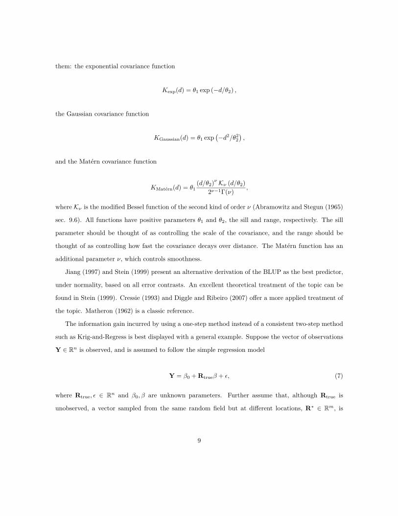
Figure 1: Map of Indonesia. Geographic location of rainfall measurements (blue) and survey data(red) merged in the Maccini and Yang (2009) analysis.
1 Introduction
Spatial data analysis has become increasingly popular in the social sciences. In many applications, data
sets providing the specific location of households, firms, villages, or other economic units are matched
by location to data with geographic features such as rainfall, temperature, soil quality, ruggedness, or
air pollution in order to analyze the impact of such environmental variables on economic outcomes.1
Such data underpins important economic research; for instance, it informs policy responses to events
such as droughts, smog outbreaks, poor harvests, etc. A typical issue is that the matched data sets will
be misaligned. That is, the respective geographical locations of the observations in the matched data
sets do not generally coincide. For instance, a researcher might observe crop outputs from a sample
of farms in a large area, as well as measurements of rainfall collected over the same area from several
weather stations. The locations of the weather stations and the farms will generally not coincide,
which yields a misaligned data set.
The approaches commonly used in social sciences to address the misalignment problem yield inef-
ficient estimates and incorrect confidence intervals. Popular approaches for analyzing such data sets
involve imputing a level of the spatial regressor for each misaligned observation of the outcome variable,
and then proceeding with standard regression analysis. It is common to impute using either the value1Maccini and Yang (2009), Miguel et al. (2004), and Shah and Steinberg (2013) study the impact of rainfall. Dell
et al. (2014) survey applications using weather data. Kremer et al. (2015) use measurements of soil nutrients in some
locations to make fertilizer recommendations in others. Nunn (2012) uses terrain ruggedness for identification, and Chay
and Greenstone (1999) study the impact of air pollution.
2

of the nearest location (Acemoglu et al. (2001)), the value of the nearest location instrumented with
more distant locations (Maccini and Yang (2009)), or a distance-weighted average of nearby locations
(Shah and Steinberg (2013)). Because these methods impute the regressors in an initial step before
considering the outcome data, I refer to them as “two-step”, or “plug-in”, methods. These estimates
are ine�cient because they do not use all the relevant information (see subsection 2.1). In addition,
confidence intervals are typically erroneous because they do not account for the fact the some covariates
have been estimated.
Gaussian maximum likelihood is a more e�cient, “one-step” method which produces accurate
point estimates. It is however known that, when erroneously assumed to be correctly specified, it
yields unreliable confidence intervals (Madsen et al. (2008)). A natural approach is then to conduct
inference using the Gaussian maximum likelihood estimator, but to dispense with the assumption
that the data follows a Gaussian distribution. The resulting estimator is called the quasi-maximum
likelihood estimate (QMLE). Even though it allows for both e�cient estimates and correct standard
errors, the QMLE is not established as the standard method for regression analysis with misaligned
data for three reasons. First, the necessary distribution theory is, to the best of my knowledge,
unavailable. Second, the computations involved are costly and di�cult. Finally, others have been
reluctant to model the covariance of the regression errors, believing it to be either too di�cult or too
restrictive.
This paper addresses each of these issues. I obtain a new central limit theorem for the QMLE with
spatial data. In particular, I present a new central limit theorem for quadratic forms in mixing variables,
which may have value in di�erent applications. I develop computational strategies to readily compute
the QMLE as well as its variance, and I assess their performance. As a robust companion method,
I suggest a minimum-distance estimator that does not require specification of the regression error
covariance. In order to conduct inference with the robust method, I obtain a new central limit theorem
for nonparametric spatial covariance function estimators, itself of independent interest. Simulations
strongly suggest that the recommended methods outperform common approaches in the literature.
I reproduce the cross-validation exercise of Madsen et al. (2008), who compare the performance for
inference of maximum likelihood with Krig-and-Regress. I find, as they did, that maximum likelihood
3

outperforms the two-step method, but that its standard errors (using the asymptotic variance formula
for correctly specified maximum likelihood) are unreliable. I find, however, that the robust standard
errors I obtain are very reliable. I reanalyze the influential data set of Maccini and Yang (2009) and
find that their general conclusions hold up: rainfall shocks in the first year of life impact adult socio-
economic outcomes. However, the analysis nevertheless benefits from the use of my methods, as those
yield some statistically and economically significant changes in the value of key parameter estimates.
It is worth noting that, even though many of the two-step methods used in the literature are in-
consistent,2 imputation with the best linear predictor in the first stage makes for a consistent estimate
of the regression coe�cient in the second stage. However, correct inference with this procedure re-
quires specification of the regression error covariance. This leaves the researcher wanting a simple, if
ine�cient, two-step method.
I propose and analyze a simple two-step Bayesian bootstrap method which, by relying on survey
sampling of the economic data in Maccini and Yang (2009), allows for a two-step method for which point
estimation and standard errors (which account for imputation uncertainty) obtain without requiring
specification of the regression error covariance.
1.1 Problem Set-Up
I now specify the general misaligned regression problem at the heart of the present inquiry. I am
interested in the regression coe�cient — in the spatial regression problem
Y = Rtrue
— + F“ + ‘, (1)
where Y = Y (x) is an N -tuple5
Y (x1
) . . . Y (xN )6T
and
Rtrue
= R(x) =5
R(x1
) . . . R(xN )6T
(2)
2All of the nearest neighbor (Acemoglu et al. (2001)), distance-weighted average (Shah and Steinberg (2013)), and
instrumental variables (Maccini and Yang (2009)) approaches produce inconsistent regression coe�cient estimates, unless
one assumes the data is getting infinitely dense asymptotically.
4

is drawn from a stationary Gaussian random field3 with mean function m(·) and covariance function
K◊(·, ·), where ◊ indexes a parametric model for the covariance function. The geographic locations are
xi œ D µ R2, i = 1, ..., N . Y and F are observed, but not Rtrue
. However, the M -tuple
Rú = R(xú) =5
R(xú1
) . . . R(xúM )
6T
, (3)
with xúi œ D µ R2, i = 1, ..., M , is observed. That is, although the outcome variable data Y (x) (e.g.
crop yields at farm locations) is not sampled at the same locations as the independent variable data
R(xú) (e.g. rain measured at fixed weather stations), it is R at the same locations as that of the
outcome variable, that is R(x), which enters the regression function.
The marginal density is then
Q
caY
Rú
R
db ≥ NN+M
Q
ca
Q
cam(x)— + F“
m(xú)
R
db ,
Q
ca—2K + � —K
—KT Kú
R
db
R
db . (4)
where K = K◊(x, x) = V◊(R(x)), K = K◊(x, xú) = Cov◊(R(x), R(xú)) and Kú = K◊(xú, xú) =
V◊(R(xú)) for some ◊ œ �.
In the absence of rainfall measurements at the locations of outcomes, the identifying assumption
is that I have a parametrized covariance function, and know Cov◊(Rtrue
, Rú) up to the value of a
small-dimensional parameter vector ◊, which I estimate consistently. This allows, for instance, the
construction of a best linear unbiased predictor for unobserved rainfall.
For my purposes, it will generally be the case that m is a constant, and thus the mean parameter
of the random field R can be absorbed in the constant vector (for the intercept) in F . Hence, I am
concerned with the marginal
Q
caY
Rú
R
db ≥ NN+M
Q
ca
Q
caF“
mú
R
db ,
Q
ca—2K + � —K
—KT Kú
R
db
R
db , (5)
3We say that
)R(x) : x œ Rd
*is a Gaussian random field if for any choice of vector of locations (x1, ..., xn), the
random vector (R(x1), ..., R(xn)) is distributed multivariate normal. The practical usefulness of Gaussian random fields
to model rainfall data has long been established, see in particular Phillips et al. (1992) and Tabios and Salas (1985).
5

where the coe�cient of interest, —, only appears in the covariance. Minus twice the log likelihood is
then
l = log!(2fi)n+m |�|" +
Q
caY ≠ F“
Rú ≠ mú
R
db
T Q
ca—2K + � —K
—KT Kú
R
db
≠1
Q
caY ≠ F“
Rú ≠ mú
R
db . (6)
If p/N is sizable, where p is the width of F , it may not be advisable to use the maximum likelihood
estimate directly. The coe�cient I am interested in is a covariance parameter in the likelihood (6),
and if a non-negligible share of the degrees of freedom is used to estimate the mean parameters, then
the estimate of the covariance may be non-negligibly biased. As explained in subsection 2.3, a natural
solution to this problem is to use a residual maximum likelihood (REML) approach.
1.2 Related Literature
My paper contributes to several segments of the literature. First and foremost, I provide methods4 for
applied researchers. As detailed above, even careful applied work (Maccini and Yang (2009), Shah and
Steinberg (2013)) relied on ad hoc approaches because econometric methodology had not caught up to
the needs of applied economists. My paper fills that gap. It speaks to a well-established literature on
generated regressors (Pagan (1984), Murphy and Topel (1985)), and looks at problems in which the
law of the regressor to impute is well described by a Gaussian random field, which makes for a rich
structure. Gaussian random fields are well studied in geostatistics (Gelfand et al. (2010), Stein (1999))
where, however, interest is concentrated on interpolation. My paper relates the two literatures and
leverages geostatistical methodology and results to provide robust and e�cient methods for economists
carrying out regression analysis with misaligned data.
The asymptotic distribution I obtain for the QMLE extends available limit distribution theory for
maximum likelihood in the spatial setting. Watkins and Al-Bouthiahi (1990) had given the asymptotic
distribution of the MLE when only the covariance function was misspecified. I give the distribution of
the MLE when both the normal distribution and the covariance function are misspecified.
The central limit theorem I obtain for inference with my minimum-distance estimator builds on4And soon, statistical packages.
6
results in spatial statistics. Cressie et al. (2002) gave a central limit theorem for empirical covariance
estimators when the data is on a lattice. I leverage results from Lahiri (2003), who gives a family of
central limit theorems for spatial statistics, in order to extend the asymptotic theory for the empirical
covariance estimators to the case of irregular spaced data.
1.3 Outline
The remainder of the article is divided as follows. Section 2 presents and discusses key concepts
and assumptions for the analysis. Section 3 develops the limit distribution theory and computational
strategies for the QMLE. Section 4 introduces a robust companion method, which circumvents the
need to model the covariance of the regression errors, and develops limit distribution theory for the
estimator. Section 5 presents the two-step Bayesian bootstrap estimator and studies its performance
in a simulation study. Section 6 studies the comparative performance of the considered estimators in
the cross-validation exercise of Madsen et al. (2008). Section 7 reanalyzes the misaligned data set
in Maccini and Yang (2009). Section 8 discusses and concludes. Technical proofs are deferred to the
appendix.
2 Key Concepts and Background Material
I introduce a few concepts playing a pivotal role in the study. First, I develop on the di�erence between
one-step and two-step methods, and give an intuitive explanation of the e�ciency gain one obtains
from the latter. Second, I define and characterize the quasi-maximum likelihood estimator (QMLE).
Finally, I define and explain the residual maximum likelihood estimator (REML).
2.1 One-step and Two-step methods
Two-step methods for regression analysis of misaligned data consist in first predicting the misaligned
covariates at the outcome locations where they are not observed, thus generating an aligned data
set, and then proceeding to standard spatial regression analysis with this generated data set.5 The5Note that Maccini and Yang (2009) do suggest a covariance estimator which accounts for the interpolation step by
using 2SLS standard errors.
7

first step, which consists of predicting the missing independent variables, requires the choice of an
interpolation method. Nonparametric methods, such as approximation by the average of a given
number of nearest neighbors, may be used. However, when the misaligned variable can be modeled
following, or approximately following, the law of a Gaussian random field, Kriging generally a�ords
the researcher more accurate interpolated variables (Gelfand et al. (2010)).
Kriging (named after the South African mining engineer D. G. Krige) consists in using the estimated
best linear unbiased predictor for interpolation. It can be developed as follows (Stein (1999)). The
random field of interest, R, is assumed to follow the model
R(x) = m(x)T “ + Á(x),
x œ D µ R2, where Á is a mean zero random field, m is a known function with values in Rp and
“ is a vector of p coe�cients. We observe R at locations x1
, x2
, ..., xN . That is, we observe Rú =
(R(x1
), R(x2
), ..., R(xN )) and need to predict R(x0
). With “ known, the best linear predictor (BLP)
is
m(x0
)T “ + kT K≠1(Rú ≠ mú“),
where k = Cov(Rú, R(x0
)), K = Cov(Rú, RúT ) and mú = (m(x1
), m(x2
), ..., m(xN ))T . Of course,
the mean parameter is in general unknown. If “ is replaced by its generalized least-squares estimator,
“ =!MT K≠1M
"≠1 MT K≠1Rú (under the assumption that K and M are of full rank), we obtain the
best linear unbiased predictor (BLUP) for R(x0
). Again, in general, the covariance structure will be
unknown, and k and K will be replaced by estimates k and K. The resulting plug-in estimator will be
called the estimated BLUP (EBLUP). Prediction with the BLUP and EBLUP are both referred to as
Kriging. As far as this article is concerned, the covariance structures will always be a priori unknown,
and Kriging will refer to prediction with the EBLUP.
There are many choices for the covariance functions (Gelfand et al. (2010)), and I present three of
8
them: the exponential covariance function
Kexp
(d) = ◊1
exp (≠d/◊2
) ,
the Gaussian covariance function
KGaussian
(d) = ◊1
exp!≠d2/◊2
2
",
and the Matérn covariance function
KMatern
(d) = ◊1
(d/◊2
)‹ K‹ (d/◊2
)2‹≠1�(‹) ,
where K‹ is the modified Bessel function of the second kind of order ‹ (Abramowitz and Stegun (1965)
sec. 9.6). All functions have positive parameters ◊1
and ◊2
, the sill and range, respectively. The sill
parameter should be thought of as controlling the scale of the covariance, and the range should be
thought of as controlling how fast the covariance decays over distance. The Matérn function has an
additional parameter ‹, which controls smoothness.
Jiang (1997) and Stein (1999) present an alternative derivation of the BLUP as the best predictor,
under normality, based on all error contrasts. An excellent theoretical treatment of the topic can be
found in Stein (1999). Cressie (1993) and Diggle and Ribeiro (2007) o�er a more applied treatment of
the topic. Matheron (1962) is a classic reference.
The information gain incurred by using a one-step method instead of a consistent two-step method
such as Krig-and-Regress is best displayed with a general example. Suppose the vector of observations
Y œ Rn is observed, and is assumed to follow the simple regression model
Y = —0
+ Rtrue
— + ‘, (7)
where Rtrue
, ‘ œ Rn and —0
, — are unknown parameters. Further assume that, although Rtrue
is
unobserved, a vector sampled from the same random field but at di�erent locations, Rú œ Rm, is
9
observed. In this set-up, a two-step method is minimizing
L1
(f(Rú) ≠ Rtrue
) ,
in f , where L1
is some loss function, to obtain R = f(Rú), and then minimizing
L2
1Y ≠ R—
2,
where L2
is some loss function, in — to get —. A one-step method instead minimizes
L3
(f(Rú) ≠ Rtrue
, Y ≠ f(Rú)—) ,
where L3
is some loss function, jointly in f and —. That is, in the one-step method but not in the two-
step method, variation in Y will inform the choice of R (by “pushing towards” an R which minimizes
regression error).
It may be tempting to conclude that the two-step method with Kriging, by plugging in a guess of
the correct dependent variable, induces attenuation bias (also known as regression dilution). It should
be clear that, in the absence of measurement error, this is not the case. For instance, consider Kriging
then regressing with known covariance structure and known mean m © 0. The first step estimate is
R =RúCov(Rú, Rú)≠1Cov(Rú, R), and the probability limit (in n) of the two-step estimator is
plim— =Cov
1Y, R
2
Cov1
R, R2
= —Cov(R, Rú)Cov(Rú, Rú)≠1Cov(Rú, R)
Cov(R, Rú)Cov(Rú, Rú)≠1Cov(Rú, Rú)Cov(Rú, Rú)≠1Cov(Rú, R)= —.
That is, the estimator is consistent. In general, m as well as the covariance structure are unknown and
have to be estimated. This will make the estimate less precise or even biased, but it does not generally
introduce attenuation bias.
10

To be sure, although two-step methods commonly used in the literature (e.g. nearest neighbors,
IV) are not in general consistent, Krig-and-Regress is a consistent two-step method. However, Krig-
and-Regress remains ine�cient as it omits information which is relevant to the estimation of — and
thus allows for a more statistically e�cient estimate. Since economists often estimate small e�ects (e.g.
the impact of rainfall in infancy on adult socio-economic outcomes), it may be crucial for estimation,
even with large data sets, that they have access to a one-step, e�cient method.
The natural candidate for a one-step method is maximum likelihood. A Gaussian likelihood function
may be preconized as it is computationally as well as analytically tractable, and in particular allows
trivial marginalization of the aligned, but unobserved variables (e.g. rainfall at the locations of the
farms). Furthermore, the likelihood approach will take into account covariance parameter uncertainty,
and can thus be expected to generate more accurate standard errors.
I am interested in the comparative performance of the maximum likelihood with two-step methods,
in particular when using Kriging in the first step. Madsen et al. (2008) study the problem of misaligned
regression and compare the maximum likelihood approach with the two-step approach consisting in first
Kriging to obtain good estimates for the missing, aligned values, and then carrying out the regression
with the interpolated quantities as “plug-in” covariates. They find that maximum likelihood yields
confidence intervals which are too narrow, and thus recommend the two-step approach as better suited
for inference. I find this to be an unpalatable conclusion. If the regression model is taken seriously,
then a two-step approach incurs e�ciency losses, and there ought to be a serious e�ort to salvage the
maximum likelihood approach.
This begs the question of how a quasi-maximum likelihood estimator with a sandwich covariance
matrix (i.e. the asymptotic covariance obtained without relying on the information equality, which
does not hold for misspecified models) would perform.
2.2 Quasi-Maximum Likelihood
In practice, even though one has recognized (perhaps transformed) data as being approximately Gaus-
sian, one often disbelieves the assumption of exact Gaussianity. Likewise, one may worry that a low-
dimensional covariance function is not flexible enough to capture the true covariance. Thus I consider
11

Figure 2: When the underlying data is not Gaussian but the mean and covariance are well specified,the QMLE ◊n is consistent. But even when the first two moments are not well specified, the QMLEhas a reasonable target ◊
0
, the parameter in the constraint set which minimizes the Kullback-Leiblerdistance to the truth.
the properties of the maximizer of the likelihood function as a quasi-maximum likelihood estimator.
That is, I will be interested in the statistical properties of the maximizer of a Gaussian likelihood
function when the data entering the likelihood is not necessarily Gaussian, or there isn’t necessarily
a parameter ◊ œ � such that K◊ gives the true covariance. I refer to this as a quasi-maximum likeli-
hood estimator (QMLE). Immediate questions, which are crucial for a cogent use of quasi-maximum
likelihood are: what is then the interpretation of the target parameter? If the covariance function is
correctly specified, are the true covariance parameters identified? Does a central limit theorem obtain?
Can we readily compute the asymptotic covariance matrix?
The last two questions will be central subjects of our inquiry, and are answered in section 3. The
first two questions can be readily answered.
For a misspecified procedure to be reasonable, we need to establish the distribution which is in fact
being estimated and decide whether or not we find it a desirable target. In many cases, the QMLE is a
consistent estimator of a very natural target. In the case of independent observations, it is well-known
(White (1982), van der Vaart (1998)) and easy to see that the limiting value of the QMLE corresponds
to the distribution within the constraint set which minimizes the Kullback–Leibler divergence with the
true distribution. As detailed below, this observation applies to dependent data as well.
12

In order to lighten notation, I use W = (W (x1
), ..., W (xn))T as the full vector of observed data. I
assume that
E[W] = 0 and Cov(W) = Vú. (8)
I am interested in the QMLE ◊(n) maximizing the Gaussian likelihood
l(W; ◊) = ≠12 log |V (◊)| ≠ 1
2WT V ≠1(◊)W, (9)
over the constraint set �, where the V (◊) = [‡(xi ≠ xj ; ◊)]i,j with explicit covariance function ‡.
To specify the target, I observe as in Watkins and Al-Boutiahi (1990) that ◊(n) = ◊0
+ op(1), with
◊0
the limiting value of the sequence {◊0
(n)} where ◊0
(n) minimizes the Kullback-Leibler distance
12 log |V (◊)| + 1
2tr!V ≠1(◊)Vú
" ≠ 12 log |Vú| ≠ n
2 , (10)
thus making ◊0
a meaningful target. Figure 2 illustrates this fact.
Now consider the case in which, although the full distribution is not correctly specified, the covari-
ance function is. Then the estimated parameter will converge to the true covariance parameter. This
follows from a direct application of the information inequality to (10), and is collected as a fact.
Fact 1 Suppose there exists ◊ú œ � such that V (◊ú) = Vú. Then (10) must be minimized at ◊0
= ◊ú.
Operationally, computing the MLE and QMLE are identical tasks. However, the inverse Fisher infor-
mation matrix does not remain a correct expression of the covariance matrix of the QMLE. To see
why that is the case, notice that under model misspecification the information equality fails to hold.
Indeed, a classical way6 of deriving central limit theorems is to use a Taylor series expansion for the
score, and obtain the sandwich covariance matrix,
H≠1IH≠1, (11)6Note, however, that under general conditions but with a well specified model, the asymptotic distribution may be
derived without the use of the information equality. See, in particular, the elegant article by Sweeting (1980).
13

where H = EQ
ˈ2
ˆ◊2
log f(W; ◊)È
and I = EQ
Ë!ˆ
ˆ◊ log f(W; ◊)"
2
È, as the asymptotic covariance when
the true underlying distribution function is Q. Then the information equality is used to simplify (11)
to the inverse Hessian H≠1(Ferguson (1996)). In the misspecified case, this cancelation does not obtain
because the information equality does not hold in general.
That is, although using the maximum likelihood estimator when the likelihood is misspecified may
give a reasonable estimate, the standard errors obtained from the inverse Hessian provide incorrect
inferential statements. This motivates inquiring into the performance of the maximum likelihood
estimate for inference when standard errors are computed using a sandwich covariance matrix.
2.3 Residual Maximum Likelihood
In the expository example (1), as well as in Madsen et al. (2008), there is only one covariate, the
misaligned one. However, in many applications, such as Maccini and Yang (2009), there may be many
other covariates, the coe�cients of which enter the mean of the distribution only. In such instances, it
will often be advisable to use residual maximum likelihood (REML) to obtain more accurate covariance
estimates.
Indeed, in economic applications, the regression component of the model may contain many control
variables. For instance, one may be using survey data in which many characteristics (gender, age,
income, district dummies, etc) are available and used as controls for each individual. If the number of
controls is large relative to the number of observations, this can induce tangible bias in the maximum
likelihood covariance estimates.
This is best illustrated with a simple example. In the standard Gaussian linear regression model
with homoskedastic variance ‡2 (conditional on X),
W ≥ N(X—, In‡2), (12)
with n observations and p control variables, the instantiation of this phenomenon is explicit. The
maximum likelihood estimator for the variance, ‡2, is biased;
14
E#‡2
$= ‡2
n ≠ p
n.
The reason, intuitively, is that p degrees of freedom are “spent” to first estimate the regression mean,
and the variance is then estimated with the residuals, which are left with n ≠ p degrees of freedom
worth of information. In the special case of the Gaussian linear model with homoskedastic variance, the
problem is readily remedied by applying a correction factor to obtain the unbiased adjusted estimator
s2 = nn≠p ‡2. However, such an immediate correction is not available in general.
A way to capture the idea that the residuals have n ≠ p degrees of freedom is to note that there
are exactly n ≠ p linearly independent error contrasts ÷j (i.e. linear transformations of Y with mean
0). In this sense, the residuals live in an n ≠ p dimensional space. Even more to the point, in the
canonical model reformulation of (12), the contrasts ÷j are obtained via the QR decomposition, and I
can explicitly express the unbiased estimator as a sum of n ≠ p random variables
s2 = 1n ≠ p
n≠pÿ
j=1
÷2
j .
The general way to proceed with REML estimation is to obtain estimates by maximizing the
likelihood of the error contrasts. The key di�erence about this approach is that it does not involve the
existence and discovery of a correcting coe�cient, and is thus applicable for our purposes.
Consider the Gaussian linear model,
W ≥ N (X–, V (◊)) ,
where Y is an n ◊ 1 data vector, X is an n ◊ p matrix of covariates, – is an unknown p-long vector of
coe�cients, and V (◊) is an n◊n positive-definite matrix known up to a vector of covariance parameters
◊ œ � open in Rk. Twice the negative log-likelihood is proportional to
log (|V (◊)|) + (W ≠ X–)T V ≠1(◊) (W ≠ X–) .
For REML, I am instead interested in maximizing the likelihood of a (in fact, any) vector of n ≠ p
15

linearly independent error contrasts. That is, I instead maximize the log-likelihood of U = �T Y for
some n ◊ (n ≠ p) matrix � satisfying �T X = 0. Clearly, U ≥ N(0, �T V (◊)�), and twice the negative
log-likelihood function based on U is proportional to
log!--�T V (◊)�
--" + UT!�T V (◊)�
"≠1
U. (13)
It is important to notice that there is no notion (or loss) of e�ciency depending on which projection
on the space of error contrasts is used. Specifically, any choice of n ≠ p linearly independent error
contrasts yields an equivalent maximum likelihood problem. Indeed, take any n ◊ (n ≠ p) matrix »
satisfying »T X = 0. Then there exists a nonsingular (n ≠ p) ◊ (n ≠ p) matrix D such that »T = D�T .
Consequently, U = »T Y has log-likelihood
log!--»T V (◊)»
--" + UT!»T V (◊)»
"≠1
U
= log!--D�T V (◊)�DT
--" + UT DT!D�T V (◊)�DT
"≠1
DU
= log!|�T V (◊)�|" + UT
!�T V (◊)�
"≠1
U + C, (14)
where C = 2 log (|D|) is a constant which depends on D but not on ◊, and hence does not a�ect the
optimization. That is, (13) and (14) yield equivalent optimization problems in ◊.
Cressie and Lahiri (1993) give a brief Bayesian justification for REML, drawing on Harville (1974).
They remark that if one assumes a noninformative prior for —, which is statistically independent of ◊,
one obtains that the marginal posterior density for ◊ is proportional to (13), multiplied by the prior for
◊. Then, if that prior is flat, the REML estimate is equivalent to the maximum a posteriori estimate.
Jiang (1997) points at another interesting connection. He observes that, under normality, the best
linear unbiased predictor for the random e�ects can be derived as the best predictor based on the
error contrasts whilst, as we have seen, REML estimates are maximum likelihood estimates for the
covariance parameters based on the error contrasts.
16

3 Quasi Maximum Likelihood Estimation
My recommendation, for the estimation problem described in (1)-(4), is to use the quasi-maximum
likelihood estimator (QMLE). In order to conduct inference with the QMLE, I obtain its asymptotic
distribution. Foregoing the Gaussianity assumption, I need instead some form of assumption guaran-
teeing that as the sample gets bigger, more information is collected. I will be using mixing assumptions,
which formalize the idea that observations farther away from each other are “more independent”. Tech-
nical details regarding mixing are treated in subsection A1.
In this section, I lay out the method, theory, and computational aspects of quasi-maximum likeli-
hood with spatial data. Although my focus remains regression analysis with misaligned data, remark
that the central limit theory developed in subsection 3.1 applies generally to, and is novel for, quasi-
maximum likelihood estimation with mixing data.
3.1 Limit Distribution Theory
I derive the asymptotic distribution of the maximum likelihood estimator of the Gaussian density under
assumptions of weak dependence on the true underlying distribution function Q. I consider the general
case (9), which encompasses (6) as well as REML. The main result of this section, given additional
technical conditions detailed in subsection A.1, is :
Assume W = (W1
, W2
, ..., Wn) is strongly mixing of size -1 with E[W ] = 0 and Cov(W ) =
Vú. The random function l : � æ R is the Gaussian likelihood function
l(W ; ◊) = ≠12 log |V (◊)| ≠ 1
2W T V ≠1(◊)W.
Let ◊ denote its maximand, the quasi-maximum log-likelihood estimator, and define the
target parameter ◊0
to be the minimizer in (10). Then
Ôn
1◊ ≠ ◊
0
2dæ N
!0, H≠1IH≠1
",
where H = EQ
ˈ2l
ˆ◊ˆ◊T (◊0
)È
and I = VQ
!ˆlˆ◊ (◊
0
)", in which EQ and VQ stand for the
17
expectation and variance taken with respect to the true underlying distribution function Q.
The proof strategy is similar to that of Jiang (1996) and relies on a useful decomposition for the
quadratic form in the score ˆl/ˆ◊. For Jiang, who deals with quadratic forms in a vector of inde-
pendent data, the decomposition gives a martingale, which he shows satisfies the su�cient conditions
of a martingale central limit theorem (Hall and Heyde, 1980, theorem 3.2). Correspondingly, I have
quadratic forms in a vector of weakly dependent data, and will show that they can be represented in
the same decomposition as mixingales, which satisfy the su�cient conditions of a mixingale central
limit theorem (de Jong, 1997).
The score for the likelihood of ◊ œ � µ Rq given in (9) is
ˆl
ˆ◊= ≠1
2tr!V ≠1V◊i
"i≠ 1
2!W T V ◊iW
"i
where (ai)i = (a1
, ..., aq)T , and V◊i and V ◊i are the derivatives with respect to ◊i of V and V ≠1,
respectively. Assuming ◊(n) Pæ ◊0
, Taylor series expansion yields
0 = ˆl
ˆ◊(◊
0
) + (◊(n) ≠ ◊0
)T ˆ2l
ˆ◊ˆ◊T(◊
0
) + Op(1),
which implies
◊(n) = ◊0
≠3
E
5ˆ2l
ˆ◊ˆ◊T(◊
0
)64≠1
ˆl
ˆ◊(◊
0
) + op(n≠1/2).
Assume the posited covariance function is well behaved enough that
3E
5ˆ2l
ˆ◊ˆ◊T(◊
0
)64≠1
Vú
3E
5ˆ2l
ˆ◊ˆ◊T(◊
0
)64≠1
= O(n≠1),
where Vú = Cov(W ). Then in order to obtain the limiting distribution for ◊(n), I need to obtain the
limit distribution for the score ˆlˆ◊ (◊
0
). Note that E#
ˆlˆ◊ (◊
0
)$
= 0 and thus
≠2 ˆl
ˆ◊(◊
0
) =!W T V ◊iW ≠ EW T V ◊iW
"i.
18
Asymptotic normality of multivariate random variables can be demonstrated using the Cramér-Wold
device. For a given t œ Rq\{0}, letting Z = V ≠1/2
ú W ,
≠tT ˆl
ˆ◊(◊
0
) = tT!W T V ◊lW ≠ EW T V ◊lW
"l
= tT!ZT AlZ ≠ EZT AlZ
"l
=ÿ
i
Q
aaii
!Z2
i ≠ E#Z2
i
$"+ 2
ÿ
j<i
aij (ZiZj ≠ E [ZiZj ])
R
b ,
where Al = V 1/2
ú V ◊lV 1/2
ú and aij =qq
l=1
tlAlij , ’ i, j with Al. Letting
Xn,i = aii
!Z2
i ≠ E#Z2
i
$"+ 2
ÿ
j<i
aij (ZiZj ≠ E [ZiZj ]) , (15)
I can write the quadratic form as
≠tT ˆl
ˆ◊(◊
0
) =nÿ
i=1
Xn,i.
Defining
Fn,i = ‡ (Zn1
, ..., Zn,i) , 1 Æ i Æ kn, (16)
I show that {Xn,i, Fn,i}, 1 Æ i Æ kn is an array of mixingales. This is an important observation
because it will allow me to use a mixingale central limit theorem to derive the limit distribution of the
score, and thus of the quasi-maximum likelihood estimator.
Definition 1 A triangular array {Xn,i, Fn,i} is an L2
-mixingale of size ≠⁄ if for m Ø 0
ÎXn,i ≠ E [Xn,i| Fn,i+m]Î2
Æ an,iÂ(m + 1),
ÎE [Xn,i| Fn,i≠m]Î2
Æ an,iÂ(m),
19

and Â(m) = O(e≠⁄≠Á) for some Á > 0. We call the an,i mixingale indices.
The mixingale CLT requires that the mixingale be of size ≠1/2, which in turn implies a requirement
on the rate of decay of the dependence for variables in the random field.
Lemma 2 Suppose that {Zn,i, Fn,i} is an –-mixing sequence of size -1 and that all Zn,i’s have a fourth
moment. Then the triangular array {Xn,i, Fn,i} defined in (15) and (16) is an L2
-mixingale of
size ≠1/2.
The proof is deferred to the appendix.
3.2 Computational Aspects
When computing the sandwich covariance formula H≠1IH≠1 obtained in subsection 3.1, some chal-
lenges need to be dealt with. Estimation of H≠1 is standard and must be done in the well-specified
case. It is in fact an even lighter task when the covariance functions are modeled since a closed form
for H immediately obtains. It is the estimation of I which raises new challenges.
Indeed, computing the variance of the score may at first seem daunting, even a motivation for
sticking with the Hessian as a covariance estimate. In particular, it involves the estimation of fourth-
order moments. The di�culty arises from the computation of the covariance of entries of the score
corresponding to covariance model parameters. For two such parameters ◊l and ◊m (say, the sill of the
rain covariance function and the range of the regression error covariance function) we have
E
5dl
d◊l(◊
0
) dl
d◊m(◊
0
)6
= 14E
#!W T V ◊lW ≠ E
#W T V ◊lW
$" !W T V ◊mW ≠ E
#W T V ◊mW
$"$
= 14
ÿ
i,j
ÿ
iÕ,jÕ
V ◊li,jV ◊m
iÕ,jÕ (E [WiWjWiÕWjÕ ] ≠ E [WiWj ] E [WiÕWjÕ ]) ,
where the dependence on fourth-order moments is made explicit.
The problem of approximating and estimating the asymptotic variance is divided into two cases, de-
pending on the robustness concerns. If the main concern is that the covariance function is misspecified,
then a fruitful approach is to keep with the quasi-Gaussian mindset, and estimate the fourth-order
20
moments using the Gaussian formula. The more important case, however, is that in which the re-
searcher is not confident that the Gaussian assumption is a tenable one. Then robustness concerns
call for estimation of the fourth-order moments. In order to accomplish that, I provide a shrinkage
estimator inspired from the finance literature.
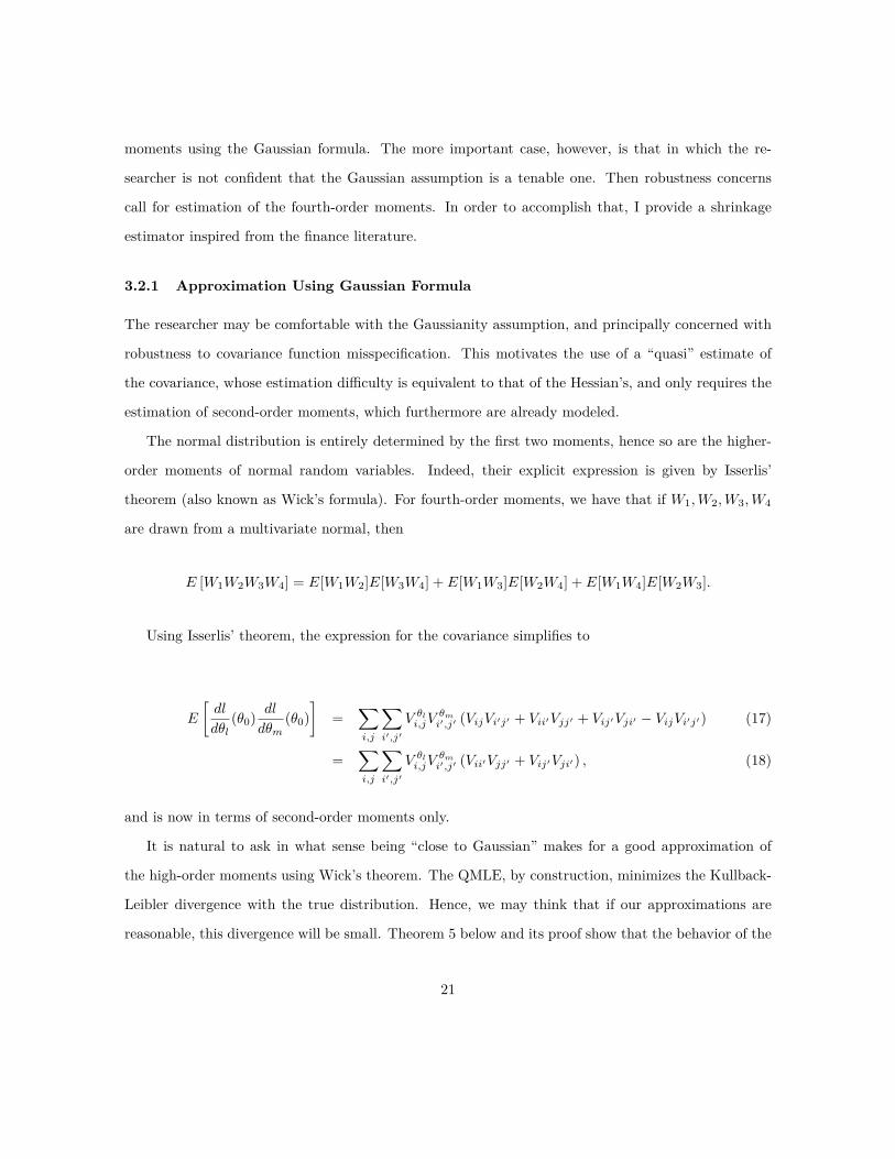
3.2.1 Approximation Using Gaussian Formula
The researcher may be comfortable with the Gaussianity assumption, and principally concerned with
robustness to covariance function misspecification. This motivates the use of a “quasi” estimate of
the covariance, whose estimation di�culty is equivalent to that of the Hessian’s, and only requires the
estimation of second-order moments, which furthermore are already modeled.
The normal distribution is entirely determined by the first two moments, hence so are the higher-
order moments of normal random variables. Indeed, their explicit expression is given by Isserlis’
theorem (also known as Wick’s formula). For fourth-order moments, we have that if W1
, W2
, W3
, W4
are drawn from a multivariate normal, then
E [W1
W2
W3
W4
] = E[W1
W2
]E[W3
W4
] + E[W1
W3
]E[W2
W4
] + E[W1
W4
]E[W2
W3
].
Using Isserlis’ theorem, the expression for the covariance simplifies to
E
5dl
d◊l(◊
0
) dl
d◊m(◊
0
)6
=ÿ
i,j
ÿ
iÕ,jÕ
V ◊li,jV ◊m
iÕ,jÕ (VijViÕjÕ + ViiÕVjjÕ + VijÕVjiÕ ≠ VijViÕjÕ) (17)
=ÿ
i,j
ÿ
iÕ,jÕ
V ◊li,jV ◊m
iÕ,jÕ (ViiÕVjjÕ + VijÕVjiÕ) , (18)
and is now in terms of second-order moments only.
It is natural to ask in what sense being “close to Gaussian” makes for a good approximation of
the high-order moments using Wick’s theorem. The QMLE, by construction, minimizes the Kullback-
Leibler divergence with the true distribution. Hence, we may think that if our approximations are
reasonable, this divergence will be small. Theorem 5 below and its proof show that the behavior of the
21

tails also matters for the approximation of fourth-order moments with Wick’s formula to be reasonable.
One way to speak of the tail behavior of a random variable is to compare it to that of Gaussian random
variables. In particular, we will say that a random variable is sub-Gaussian if its tails are dominated
by those of some Gaussian random variable.
Definition A mean-zero random variable X is sub-Gaussian with parameter ‹2 if, for all ⁄ œ R,
E#e⁄X
$ Æ exp3
⁄2‹2
2
4.
I now give a theorem characterizing conditions under which the moment approximation is tenable.
Theorem 5 Consider a sequence of pairs of distributions {(Pi, Fi)} for which
DKL(Fi||Pi) æ 0, (19)
as i æ Œ, where DKL(F ||P ) =´
ln dFdP dF is the Kullback-Leibler divergence. Further suppose that
the Pi, i = 1, 2, ... are sub-Gaussian of some given parameter. Let the N -tuple Y = Y (n) follow
distribution Pn and the N -tuple X = X(n) be Gaussian with distribution Fn. Then
|E[YiYjYkYl] ≠ (E[XiXj ]E[XkXl] + E[XiXk]E[XjXl] + E[XiXl]E[XjXk])| æ 0, (20)
1 Æ i, j, k, l Æ N , as n æ Œ.
The proof is given in the appendix, and consists in getting a multivariate Pinsker inequality via a
residue theorem. The sub-Gaussian assumption can be replaced by an assumption of uniform integra-
bility on the moments of order 4 + ‘, for some ‘ > 0.
What comes out of the proof of Theorem 5 is that a small Kullback-Leibler distance takes care of
the bulk of the density, but we must also assume that the tails vanish in order for the fourth moments
to be close. This is particularly nice because these are two features of the data which the researcher
would inspect on a QQ-plot.
Of course, submitting this quadruple sum as a loop is prohibitively ine�cient, and should not be
22

done as such. Using the indexation, I can rearrange the formula in a computationally economical
matrix form. Simply observe that
ÿ
i,j
ÿ
iÕ,jÕ
V ◊li,jV ◊m
iÕ,jÕ (ViiÕVjjÕ + VijÕVjiÕ) =ÿ
i,j
ÿ
iÕ,jÕ
V ◊li,jV ◊m
iÕ,jÕViiÕVjjÕ +ÿ
i,j
ÿ
iÕ,jÕ
V ◊li,jV ◊m
iÕ,jÕVijÕVjiÕ
=..V ◊l ¶ !
V V ◊mV"..
sum
+...V ◊l ¶
1V
!V ◊m
"TV
2...sum
,
where ¶ is the element-wise multiplication (i.e. for A = (aij) the matrix with (i, j) entry aij and
B = (bij) defined likewise, A ¶ B = (aijbij)) and ÎAÎsum
=q
i,j aij .
To be sure, such an approach is particularly well-suited to the case of covariance misspecification.
If the main concern is distribution misspecification, fourth-order moments ought to be estimated.
3.2.2 Estimating Fourth-Order Moments
A key case is that in which first and second moments are well specified but Gaussianity is suspect. In
that case, the estimated coe�cient is consistent (e.g. the target parameter for — is the true value —),
making the QMLE particularly attractive. However, in that case, the Gaussian formula provides an
untenable approximation for the fourth-order moments, and one is well-advised to estimate them.
Estimation of fourth-order moments is di�cult. Additional assumptions and more sophisticated
methods need to be called upon in order to carry out this task. Some early approaches (Elton & Gruber
(1973)) have allowed for less volatile estimation, but at the cost of potentially heavy misspecification.
Recent strides in covariance matrix estimation have consisted in attempts to trade o� variance
and bias under some optimality criterion. In particular, Ledoit and Wolf (2003) suggested a shrinking
estimator, and gave a theoretically founded optimal shrinkage parameter which has an empirical analog.
Martellini and Ziemann (2010) have extended these results to higher-order moment tensors. Both
articles had their applications in finance.
I extend the method displayed in Martellini and Ziemann (2010), and like them rely on the theory
developed in Ledoit and Wolf (2003) to suggest a shrinkage estimator for fourth-order moments.
In order to get some level of replication with spatial data, I must make stationarity assumptions.
23
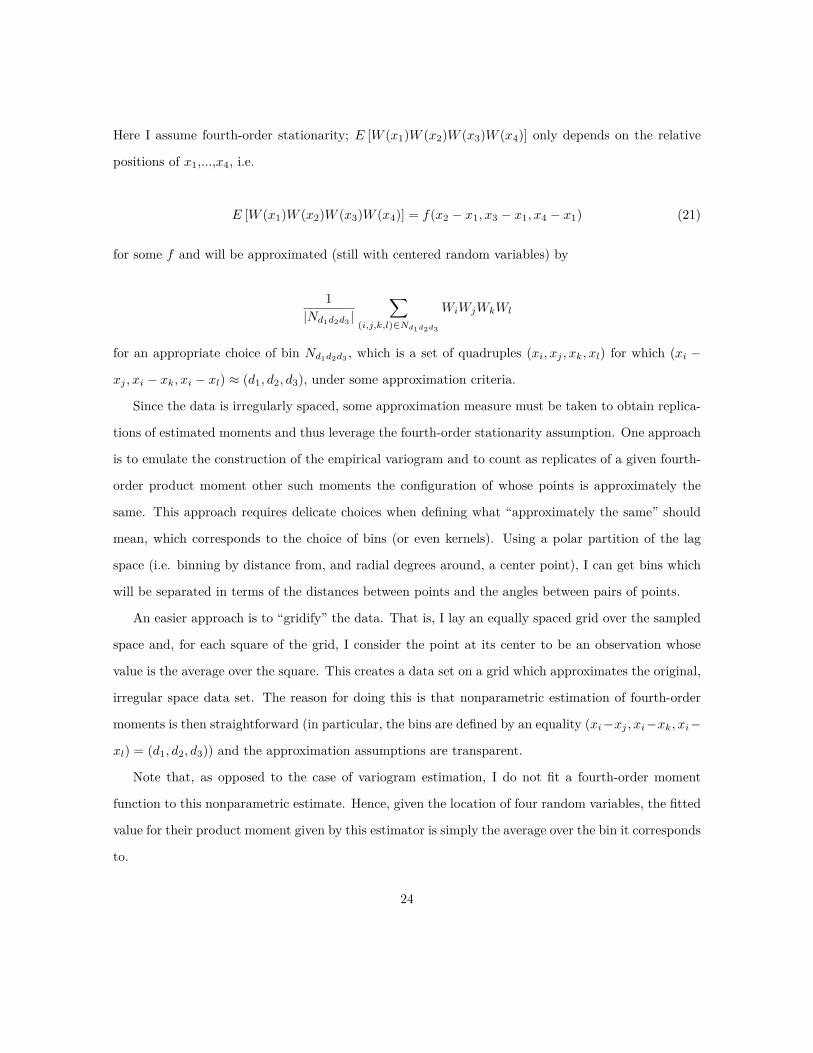
Here I assume fourth-order stationarity; E [W (x1
)W (x2
)W (x3
)W (x4
)] only depends on the relative
positions of x1
,...,x4
, i.e.
E [W (x1
)W (x2
)W (x3
)W (x4
)] = f(x2
≠ x1
, x3
≠ x1
, x4
≠ x1
) (21)
for some f and will be approximated (still with centered random variables) by
1|Nd
1
d2
d3
|ÿ
(i,j,k,l)œNd1
d2
d3
WiWjWkWl
for an appropriate choice of bin Nd1
d2
d3
, which is a set of quadruples (xi, xj , xk, xl) for which (xi ≠xj , xi ≠ xk, xi ≠ xl) ¥ (d
1
, d2
, d3
), under some approximation criteria.
Since the data is irregularly spaced, some approximation measure must be taken to obtain replica-
tions of estimated moments and thus leverage the fourth-order stationarity assumption. One approach
is to emulate the construction of the empirical variogram and to count as replicates of a given fourth-
order product moment other such moments the configuration of whose points is approximately the
same. This approach requires delicate choices when defining what “approximately the same” should
mean, which corresponds to the choice of bins (or even kernels). Using a polar partition of the lag
space (i.e. binning by distance from, and radial degrees around, a center point), I can get bins which
will be separated in terms of the distances between points and the angles between pairs of points.
An easier approach is to “gridify” the data. That is, I lay an equally spaced grid over the sampled
space and, for each square of the grid, I consider the point at its center to be an observation whose
value is the average over the square. This creates a data set on a grid which approximates the original,
irregular space data set. The reason for doing this is that nonparametric estimation of fourth-order
moments is then straightforward (in particular, the bins are defined by an equality (xi ≠xj , xi ≠xk, xi ≠xl) = (d
1
, d2
, d3
)) and the approximation assumptions are transparent.
Note that, as opposed to the case of variogram estimation, I do not fit a fourth-order moment
function to this nonparametric estimate. Hence, given the location of four random variables, the fitted
value for their product moment given by this estimator is simply the average over the bin it corresponds
to.
24

I call the resulting nonparametric estimator S. I want to stabilize the estimator S. A stable but
potentially misspecified fourth-order moment tensor is obtained by replacing each fourth-order moment
by its Gaussian expression (in terms of second-order moments). I call this tensor the Isserlis tensor,
and label it �. The shrinkage estimator I propose is
–� + (1 ≠ –)S.
The critical step is then the choice of the tuning parameter –.
Ledoit and Wolf (2003) give a theoretically founded approach for picking – when dealing with
covariance matrices, and Martellini and Ziemann (2010) extend the approach to deal with tensors of
higher order moments. I follow their approach.
The suggested parameter is
– = 1N
fi
“,
where fi =q
ijkl fiijkl and “ =q
ijkl “ijkl, with
fiijkl = 1|Nd
1
d2
d3
|ÿ
(i,j,k,l)œNd1
d2
d3
(WiWjWkWl ≠ Sijkl)2
as the sample variance of the tensor, and
“ijkl = (�ijkl ≠ Sijkl)2
is the sample squared error of the structured estimator.
Martellini and Ziemann (2010) suggest accounting for the covariance between entries of S and � by
adding a covariance estimate term in the numerator. However, this is a di�cult quantity to estimate,
and since � is an order of magnitude less variable than S, I feel comfortable omitting that term so to
propose a much simpler procedure.
An approximation which I recommend considering is the use of the Gaussian formula for the fiijkl’s.
It gives weights in terms of a sensible function of the configuration, and avoids the rather hopeless
25

0.0 0.2 0.4 0.6 0.8 1.0
0.0
0.2
0.4
0.6
0.8
1.0
Figure 3: Simulated Gaussian random Field, with range parameter 0.15.
reliance on estimated eighth moments (especially since the motivation for using shrinkage in the first
place is the high variance of the fourth moments).
The next order of business is to assess the performance of the nonparametric and shrinkage es-
timators. I assess the performance of the estimators by considering cases in which I can compare
estimated fourth-order moments with their correct values. For Gaussian random variables, the value
of fourth-order moments is obtained in closed form using Wick’s formula (since I have closed forms
for the covariances) and thus the comparison is readily made. Figure 3 presents a heat map of the
simulated Gaussian random field.
To visualize and compare the estimated fourth moments with the true ones, I present plots con-
structed as follows. Each plot presents the complete estimation domain (e.g. the geographical area
under study). I fix the location of three of the four points whose fourth-order product moment I
estimate (and indicate the location of those three points on the plot, some may overlap). The value
at each location on the plot is that of the fourth-order product moment (true or estimated, depending
on the plot) whose fourth point is at that location.
From inspection of figures 4 and 5, we can see that the approximation is good near the location of
26

0.0 0.2 0.4 0.6 0.8 1.0
0.0
0.2
0.4
0.6
0.8
1.0
0.0 0.2 0.4 0.6 0.8 1.0
0.0
0.2
0.4
0.6
0.8
1.0
Figure 4: Plot of fourth-order moment E[W (x1
)W (x2
)W (x3
)W (x4
)] as a function of the position x4
with x1
= x2
= x3
= (0.5, 0.5) and range parameter 0.15. The left-hand side figure gives the contourplot of the true moment. The right-hand side figure gives the contour plot of the nonparametricestimates.
the three fixed points, and deteriorates farther away from them. This further suggests that, although
it is beneficial to leverage the nonparametric estimator for its robustness, embedding it in a shrinkage
estimator may make for a more satisfactory method.
We can see from figure 5 that shrinkage helps attenuate the more erratic behavior of the nonpara-
metric fourth-moment estimator. The undesired local maxima are repressed, and the contours around
the true local maxima are better behaved.
4 Robust Estimation
Specification of the covariance model for the regression errors is arguably the most onerous assumption
the researcher needs to make. One may worry that the regression error covariance does not have the nice
structure common to geophysical variables, e.g. since we ineluctably omit variables in the regression
function. This motivates an estimation scheme relieved of that specification burden.
Upon inspection of the marginal density (5), we find that — is identified from VRú = Kú and
VY Rú = —KT alone, and hence identification does not require modeling the covariance structure of
the regression errors. Specifically, using rainfall data only, one obtains an estimate of the covariance
27

0.25 0.30 0.35 0.40 0.45 0.50 0.55 0.60
0.2
0.3
0.4
0.5
0.6
0.25 0.30 0.35 0.40 0.45 0.50 0.55 0.60
0.2
0.3
0.4
0.5
0.6
0.25 0.30 0.35 0.40 0.45 0.50 0.55 0.60
0.2
0.3
0.4
0.5
0.6
Figure 5: Plot of fourth-order moment E[W (x1
)W (x2
)W (x3
)W (x4
)] as a function of the position x4
,with x
1
= x2
= (0.5, 0.5), x3
= (0.4, 0.4) and range parameter 0.05. The left-hand side figure givesthe contour plot of the true moments. The middle figure gives the contour plot of the nonparametricestimates. The right-hand side plot gives the contour plot of the estimates using shrinkage.
parameter ◊, and thus has an estimate of K. Since —K is directly identified from the covariance
between the outcome data and the observed rain, — is identified. This naturally invites a procedure
which will rely on this identification observation to yield a robust estimate of —. In this section, I lay
out such a procedure.
I develop a robust estimation method for the regression coe�cient. In order to conduct inference,
I develop limit distribution for the robust estimator. The limit distribution theory (in particular
the central limit theorem for the moment vector with irregular spaced data and increasing domain
asymptotics), however, is useful and novel in the general case.
4.1 Methodology
Let “Rú(d; ◊) = V◊(R(x) ≠ R(x + d)) and “Y Rú(d; ◊) = V◊(R(x) ≠ Y (x + d)) be the variogram of Rú
and the covariogram of Y with Rú, respectively. Note that “Y Rú(d; ◊) = —“Rú(d; ◊). Let “úRú(d) and
“úY Rú(d) be generic, nonparametric estimators of “Rú(d; ◊) and “Y Rú(d; ◊), respectively.
Let {c1
, ..., cKRú } and {d1
, ..., dKY Rú } be finite sets of lags such that “úRú(di) is defined for all
28
i = 1, ..., KRú and “úY Rú(cj) is defined for all j = 1, ..., KY Rú .7 Let „ = (—, ◊) and
gn(◊) = 2 (“úY Rú(d
1
) ≠ “Y Rú(d1
; ◊), · · · , “úY Rú(dK) ≠ “Y Rú(dKY Rú ; ◊),
“úRú(c
1
) ≠ “Rú(c1
; ◊), . . . , “úRú(cKRú ) ≠ “Rú(cKRú ; ◊)) .
For some positive-definite weighting matrix Bn, define
◊Robust
= arg min◊œ�
)gn(◊)T Bngn(◊)
*.
Then —Robust
, the estimate of —, does not depend on any specification of the covariance structure of the
regression errors. Di�erent choices of Bn will correspond to di�erent traditional estimators; Bn = I
yields the ordinary least squares estimator, Bn = diag(bn,1(◊), ..., bn,KY Rú +KRú (◊)), for some choice of
weights bn,i, i = 1, ..., K, gives the weighted least squares estimator, and Bn(◊) = �≠1
“ (◊), where �“(◊)
is the asymptotic covariance matrix of 2 (“úY Rú(c
1
), · · · , “úRú(dKY Rú ))T is the generalized least-square
version of the minimum-distance estimator.
Another attractive feature of this estimator is its flexibility. The vector of moments can be extended
to accommodate other conditions, perhaps motivated by economic theory.
4.2 Limit Distribution Theory
In order to carry out inference using the proposed minimum distance estimator, I need asymptotic
distribution theory for the statistic, that is the empirical variogram (defined below). Cressie et al.
(2002) give such a theorem in the case in which the data is on a lattice, and even give the asymptotic
distribution of the minimum distance estimator as a corollary. Lahiri (2003) proves a series of very
useful central limit theorems for spatial statistics, one of which can be leveraged to extend the asymp-
totic theory for the empirical variogram to the case of irregular data. I give this result in the present
section.7The lags can be the default lags of the empirical variogram estimator from a geostatistical package, such as gstat.
29

Let the empirical variogram (Gelfand et al. (2010) p.34) be defined
“(h) = 1|Nn(h)|
ÿ
(si,sj)œNn(h)
(Á(si) ≠ Á(sj))2 ,
where the bin Nn(h) is the set of pairs of observations separated by a distance close to h, which I have
chosen to approximate “(h, ◊0
).
In spatial econometrics and statistics, limit distribution theory depends on the asymptotic domain
chosen by the analyst. One may consider the pure-increasing domain (more and more points, always
at a minimum distance from each other), infill asymptotics (more and more points in a fixed, finite
area), or a mix of the two (points get denser and over a wider area as their number increases). The
data sets analyzed herein have many observations, generally distant from each other (measured both
by geographic distance and correlation), which is typical for social science applications (as opposed to
mining or medical imaging). Hence, to best capture these features of the data, all asymptotics in this
article are done in the pure-increasing domain.
The limit distribution theory can be obtained in the pure-increasing domain, with the so-called
stochastic design (Lahiri (2003)). Explicitly, the sampling region is denoted Rn, and is for each n a
multiple of a prototype region R0
, defined as follows. The prototype region satisfies Rú0
µ R0
µ Rú0
,
where Rú0
is an open connected subset of (≠1/2, 1/2]d containing the origin. Let {⁄n}nœN be a sequence
of positive real numbers such that n‘/⁄n æ 0 as n æ Œ for some ‘ > 0. Then the sampling region is
defined as
Rn = ⁄nR0
.
To avoid pathological cases, I will assume that the boundary of R0
is delineated by a smooth function.
This assumption can be modified and weakened to adapt to other domains (e.g. star-shaped ones),
see Lahiri (2003).
Furthermore, we speak of a stochastic design because the data is not placed on a lattice, and obser-
vation locations must be modeled otherwise. They are modeled as follows. Let f(x) be a continuous,
everywhere positive density on R0
, and let {Xn}n be a sequence of independent and identically dis-
30

tributed draws from f . Let x1
, ..., xn be realizations of X1
, ..., Xn, and define the locations s1
, ..., sn of
the observed data in Rn as
si = ⁄nxi, i = 1, ..., n.
In the stochastic design, pure-increasing asymptotics require that n/⁄2
n æ C for some C œ (0, Œ)
as n æ Œ.
First, I obtain a central limit theorem for the statistic entering the minimum distance objective
function. For simplicity, take gn as defined above but let {d1
, ..., dK}, K œ N, be the full set of lags.
Recall that m and m are the mean and estimated mean, respectively, of the random field (e.g. of
rainfall).
Theorem 6 Suppose that f(x) is continuous and everywhere positive on R0
and that ⁄2
n Îm ≠ mÎ4
2
=
op(1). Further assume that E |R(0)|4+” < Œ and for all a Ø 1, b Ø 1, –(a, b) Æ Ca≠·1b·
2 for
some 0 < ” Æ 4, C > 0, ·1
> (4 + d)/”, and 0 Æ ·2
< ·1
/d. Then if n/⁄2
n æ C1
,
n1/2gn(◊0
) æ N (0, �g(◊0
)) ,
where the i, j entry of the covariance matrix is [�g(◊0
)]i,j = ‡ij(0) + Q · C1
· ´R2
‡ij(x)x, with
Q =´
Rnf2(s)ds and ‡ij(x) = Cov◊
0
1(R(0) ≠ R(di))2 , (R(s) ≠ R(x + dj))2
2.
With the limit distribution of the statistic in hand, the central limit distribution of the minimum
distance estimator obtains.
Theorem 7 Suppose that f(x) is continuous and everywhere positive on R0
and that ⁄2
n Îm ≠ mÎ4
2
=
op(1). Further assume that E |R(0)|4+” < Œ and for all a Ø 1, b Ø 1, –(a, b) Æ Ca≠·1b·
2 for
some 0 < ” Æ 4, C > 0, ·1
> (4+d)/”, and 0 Æ ·2
< ·1
/d. Then under the conditions cited in As-
sumption A.1, if n/⁄2
n æ C1
and the matrix of partial derivatives �(◊0
) = ≠2 (g1
(◊0
); ...; gK(◊0
))
is full rank,
n1/2(◊n ≠ ◊0
) dæ N (0, �(◊0
)) ,
where �(◊0
) = A(◊0
)�(◊0
)T B(◊0
)�g(◊0
)B(◊0
)�(◊0
)A(◊0
), A(◊0
) =!�(◊
0
)T B(◊0
)�(◊0
)"≠1.
31

The density of the observation locations f has an intuitive impact on the asymptotic covariance.
As one would expect, if the observations are well spread geographically then this makes for a lower
variance because Q =´
Rnf2(x)dx is smaller. Correspondingly, cluttered data arranged as a few
clusters provides worse information, and the variance is greater for it.
Comparison of the methods detailed in sections 3 and 4 illustrates tradeo�s facing the researcher
when estimating —. At the cost of ignoring the information about — in the covariance of the outcome
variable Y , the researcher obtains a less e�cient estimator, but one which does not require specification
of the regression error covariance �.
In many economic applications, the estimated e�ect can be weak and the e�cient method will be
preferred. In that case, the minimum distance estimator of this section provides a useful robustness
check.
5 Two-Step Bayesian Bootstrap
The main motivation for resorting to a two-step method such as Krig-and-Regress is the desire to avoid
specifying a model for the covariance of the regression errors, �. However, correct inference requires
standard errors which nevertheless take into account the uncertainty brought about by the imputation
of the missing covariates. That is, one needs a two-step estimator for which neither estimation nor
inference requires knowledge of �, and whose standard errors account for the uncertainty in the first
step.
Let D µ R2 be the geographic domain under study. Let R and Y be the random fields for
rainfall and the outcome variable (say height), respectively. Let Xú be the (fixed) locations of the
rainfall measurement stations. Let R = Eú[R|Rú], where Eú is the best linear prediction operator and
Rú = R(Xú) is the interpolated rainfall. Let X be the (random) locations of surveyed households.
The key observation is that if all the uncertainty in the second step arises from the resampling
(with replacement) of the surveyed households, then the observations are independently distributed,
conditional on the realization of R and Y . That is, conditional on the realization of the random
field of rainfall and the outcome variable at all households (but unconditional on which household
32

is randomly drawn with replacement from the population), the observations are independent and
identically distributed.
I believe the assumption of resampling with replacement is innocuous. Certainly, sampling without
replacement describes more accurately the sampling protocol of the survey. Nevertheless, the survey
size is so small compared to the population size that both sampling methods (with and without
replacement) yield the same sample with overwhelming probability.
5.1 Inference
The researcher may conclude that modeling the covariance of the regression errors is too restrictive.
For instance, specification of di�erent but equally credible covariance structures may yield tangibly
di�erent estimators. The robust estimation method of section 4 then remains a viable alternative.
However, some researchers may prefer employing a two-step method.
In that case, correct inference requires standard errors which will take into account the variation
brought about by the estimation of the imputed regressor.
Versions of this problem have come up in the literature under many guises (see for instance Pagan
(1984)). A very general case was addressed by Murphy and Topel (1985), who provided an asymptotic
covariance formula with a positive-definite correction term accounting for the variation due to the
estimation of the imputed regressors.
Maccini and Yang (2009) take into account the variation due to imputation by performing inference
using two-stage least-squares. However, identification under this approach is hard to argue, and
estimates of the regression coe�cients need not be consistent (see subsection 7.2).
Madsen et al. (2008) work out standard errors for the regression coe�cient estimated using the
Krig-and-Regress method. They provide a protocol for estimating the unconditional (on the realization
of the random field for the misaligned regressor) variance of the regression coe�cient. They find, in
their application, that the produced unconditional standard errors di�er only mildly from the OLS
standard errors. Crucially, the standard errors they provide do not account for the estimation of the
covariance parameter for rainfall.
My concern, in contrast with that of Madsen et al. (2008), is not to produce variance estimates
33

for the unconditional distribution of the regression coe�cient —. My concern is to provide confidence
intervals that take into consideration the uncertainty due to the estimation of the imputed regressor.
Note that in the Krig-and-Regress method, accounting for the variation due to the estimation of the
imputed regressor is tantamount to accounting for the variance due to the estimation of the covariance
and mean parameters of the random field of rainfall.
Since the motivation for using a two-step method is to avoid the modeling burden of specifying the
covariance structure for the regression errors, I ought to produce standard errors that do not require
evaluating �. In particular, the standard errors equivalent to those provided by Murphy and Topel
(1985) would require such a specification.
It is plausible that the residual errors of the best linear predictor
Y (X) ≠ Eú[Y (X)|R(X)],
where Eú is the best linear prediction operator, are spatially correlated (for instance, through an
omitted variable such as pollution, which concentrates di�erently in di�erent areas). Uncertainty
assessments of the the Krig-and-Regress coe�cient estimates, if we do not condition on the realization
of R and Y , are thus bound to rely on the estimation of �.8
5.2 Point Estimation
To be sure, estimation of the regression error covariance � may be required for di�erent reasons. If
one wants to use the maximum likelihood one-step estimator, then one must specify the covariance
structure for the regression errors in order to specify the likelihood and proceed with estimation.
Reluctance to specify such a covariance structure may strike some researchers as an encouragement to
stick with a two-step method, in particular with a Krig-and-Regress approach. However, under some
data generating processes, e�ciency concerns may urge the specification of �, even for implementation
of a two-step method such as Krig-and-Regress. Indeed, in some instances (such as Madsen et al.
(2008), see section 6), the small sample improvements from using a feasible generalized least-squares8Unless done with standard errors so conservative that they are useless in practice.
34
approach (rather than ordinary least-squares) in the second step can be compelling. That is, even
point estimation using the two-step method Krig-and-Regress may require estimation of �.
However, if the original motivation for using a two-step estimator is to not specify �, a di�erent
two-step method must be considered.
5.3 Identification Under Survey Sampling
Importantly, one can construct a di�erent estimator which exploits di�erently the sources of random-
ness and provides correct inference without relying on knowledge of �. Both QML and Krig-and-
Regress consistently estimate Eú[Y (X)|R(X), X], where uncertainty in the regression coe�cients is
thought to capture the variation arising from repeated samples of (Y, R, X). However, I can instead
treat the problem as one of survey sampling and estimate the linear regression coe�cient of Y (X )
on R(X ) over the whole population (say, of Indonesian households) for the given realizations of the
random fields Y and R, where X is the vector of locations of all (Indonesian) households. The varia-
tion comes from the random selection of the survey households, whose locations are collected in X. If
the surveyed households are drawn with replacement from the full population, then the corresponding
observations (Yi, Ri) sampled with replacement from (Y (X ), R(X )) will be independent and identically
distributed. In particular, under survey sampling, estimation of the regression coe�cient will not rely
on the specification of �.
5.4 Two-step Bayesian Bootstrap
I present an estimator which consistently estimates the (Indonesian) population regression coe�cient
and does not require specification of � for point estimation or inference.
Let fi(◊) be the prior distribution of the rainfall covariance coe�cient ◊ (e.g. a Gaussian or an
improper uniform prior) and consider its posterior fi(◊) Ã f(Rú|◊)fi(◊).
Given ◊, and conditional on the realization of the random field of rainfall as well as the outcome
variable for each household of the population, — only depends on which households are drawn (ran-
domly, with replacement) to be part of the survey. This variation is captured by resampling using the
Bayesian bootstrap. This naturally suggests a two-step Bayesian bootstrap procedure in which ◊ is
35

Figure 6: Heat map of realization of random field of rainfall. The range parameter is 3.
first drawn from its posterior to determine R(◊), thus capturing the uncertainty due to the estimation
of ◊.
The full procedure is described in pseudocode as follows:
• For each j = 1, ..., J
– Draw ◊(j) ≥ fi(◊)
– Compute R(j) = R(◊(j))
– Generate V1
, ..., Vn as n independent draws from an exponential with scale parameter 1
– Compute —(j) by regressing (Ô
ViYi)i=1,...,n on (Ô
ViR(j)
i )i=1,...,n.
Quantiles from the set of posterior draws {—(j)}j=1,...,J can be used to form credible intervals, and the
posterior mode, mean or median can be used to give a point estimate.
5.5 Simulation
I implement the two-step Bayesian bootstrap estimator in a simulation exercise. I simulate a small
data set of 80 observations (M = 40, N = 40). The data has been generated such that the (random)
location of a household is correlated with its outcome variable. Hence, obtaining the unconditional
sampling distribution of the Krig-and-Regress estimator would require careful modeling of the covari-
ance structure of the regression errors. The true value for the regression coe�cient is — = 5.
36
β
Frequency
4.80 4.85 4.90 4.95 5.00 5.05 5.10
020
60100
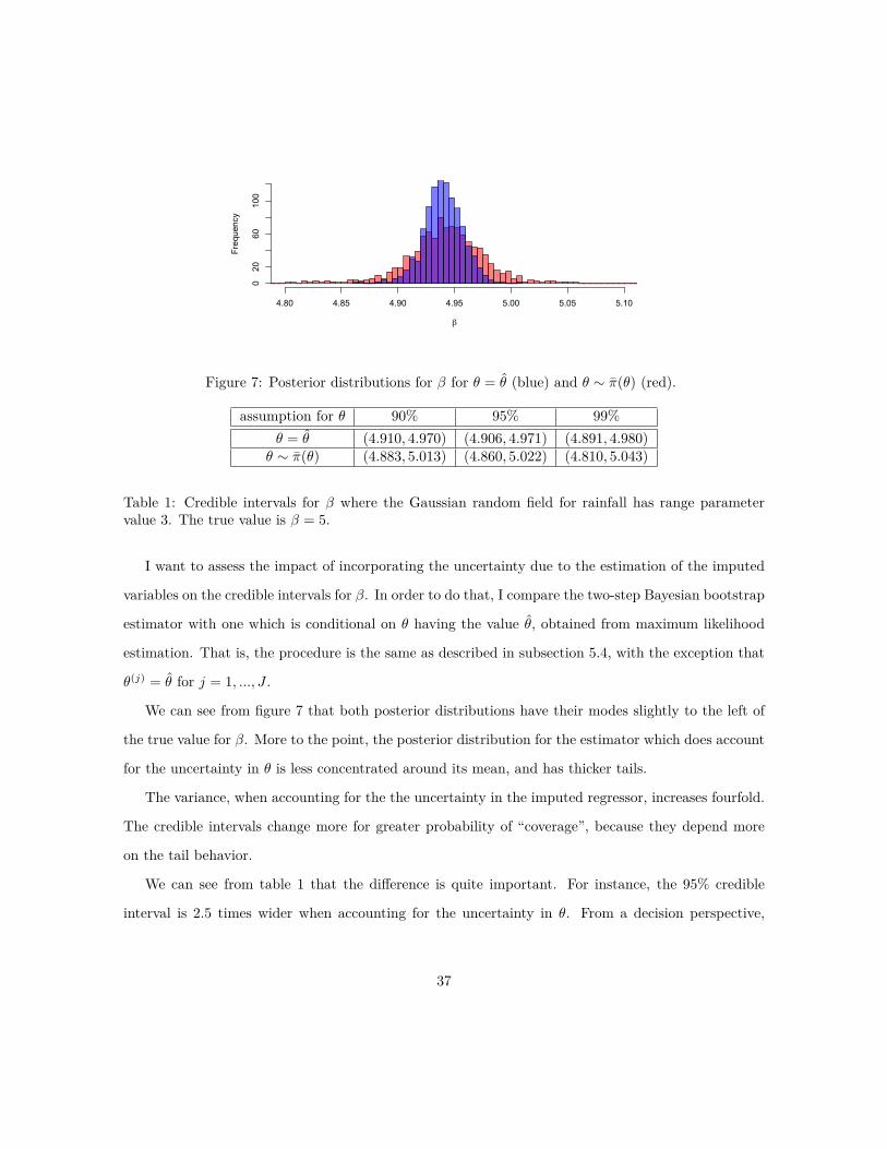
Figure 7: Posterior distributions for — for ◊ = ◊ (blue) and ◊ ≥ fi(◊) (red).
assumption for ◊ 90% 95% 99%◊ = ◊ (4.910, 4.970) (4.906, 4.971) (4.891, 4.980)
◊ ≥ fi(◊) (4.883, 5.013) (4.860, 5.022) (4.810, 5.043)
Table 1: Credible intervals for — where the Gaussian random field for rainfall has range parametervalue 3. The true value is — = 5.
I want to assess the impact of incorporating the uncertainty due to the estimation of the imputed
variables on the credible intervals for —. In order to do that, I compare the two-step Bayesian bootstrap
estimator with one which is conditional on ◊ having the value ◊, obtained from maximum likelihood
estimation. That is, the procedure is the same as described in subsection 5.4, with the exception that
◊(j) = ◊ for j = 1, ..., J .
We can see from figure 7 that both posterior distributions have their modes slightly to the left of
the true value for —. More to the point, the posterior distribution for the estimator which does account
for the uncertainty in ◊ is less concentrated around its mean, and has thicker tails.
The variance, when accounting for the the uncertainty in the imputed regressor, increases fourfold.
The credible intervals change more for greater probability of “coverage”, because they depend more
on the tail behavior.
We can see from table 1 that the di�erence is quite important. For instance, the 95% credible
interval is 2.5 times wider when accounting for the uncertainty in ◊. From a decision perspective,
37

assumption for ◊ 90% 95% 99%◊ = ◊ (4.912, 5.073) (4.898, 5.089) (4.867, 5.113)
◊ ≥ fi(◊) (4.855, 5.164) (4.830, 5.188) (4.768, 5.231)
Table 2: Credible intervals for — where the Gaussian random field for rainfall has range parametervalue 5. The true value is — = 5.
when fixing ◊ = ◊, none of the three credible intervals in table 1 include the true value — = 5, although
all of the credible intervals for the procedure drawing ◊ from fi(◊) do include the true value.
If I increase the range covariance parameter from 3 to 5, thus reducing the e�ective sample size,
all credible intervals widen, and the di�erence in credible intervals with and without accounting for
variability in ◊ remains as important.
As expected, accounting for the estimation of the imputed regressors matters tangibly for inference,
and presenting confidence or credible intervals which are in fact conditional on the estimated covariance
parameter ◊ can be misleading, especially if they are not clearly presented as such.
It should be highlighted that this estimation procedure is particularly easy. Relying on standard
Bernstein-von Mises results, the posterior fi(◊) can be approximated by a normal with mean and
covariance estimated by maximum or quasi-maximum likelihood. Then sampling ◊(j) ≥ fi(◊) is a
single line of code. The second step of the Bayesian bootstrap is then done by simply multiplying
the outcome data and interpolated data by the square root of exponential random variables, which
likewise only requires one additional line of code.
6 Revisiting Madsen, Rupert, and Altman (2008)
I apply and compare the methods under study using the cross-validation exercise of Madsen et al.
(2008). I use the same data set9 as in their article. As explained therein, and further detailed in
Herlihy et al. (1998), the data is a subset of the sample obtained for the Environmental Monitoring and
Assessment Program of the Environmental Protection Agency. All samples are from rivers and streams
in the American Mid-Atlantic region, and the analysis objective was to relate stream characteristics9I would like to thank the authors for kindly providing their data for replication.
38

distancesemivariance
1
2
3
5 10 15 20
Figure 8: Empirical and fitted variogram of R.
with land use variables. There are 558 observations over an area of 400,000 squared kilometers. The
outcome variables Y (x) are the logarithm of chloride concentration at locations x, and the dependent
variables R(xú) are the logit transformations of the per cent of watershed in forest at locations xú.
The reference value is obtained by doing generalized least-squares on the full, aligned data set
weighting with an estimate of the regression error covariance: I obtain —full
= ≠0.38. The simulation
is run as follows; for each run a randomly chosen half of the independent variables, the Ri’s, are
“hidden”, and the outcome variable, the Yi’s, are “hidden” for the other half of the data set, thus
creating a misaligned data set. For each round of the cross-validation exercise, — is estimated with
each method, and estimates are recorded.
There are two ways to carry out the second stage regression. The first is to simply do ordinary
least-square (OLS), and the second is to use feasible generalized least-squares (GLS). For the latter
approach, one obtains the weighting matrix by first fitting OLS to obtain residuals, and then fitting a
covariance function to the residuals (in this case, an exponential covariance function), thus yielding an
estimate of their covariance to use as weighting matrix. With respect to the data set of Madsen et al.
(2008), adjusting the inner products with an estimate of the covariance of the regression errors turns
out to be crucial for obtaining reliable estimates. This is a very important point and a key motivation
for adopting the survey sampling target; under resampling of Y and R, even two-step estimation of the
best linear predictor Eú[Y (X)|R(X)] may require specification of �, the covariance of the regression
39
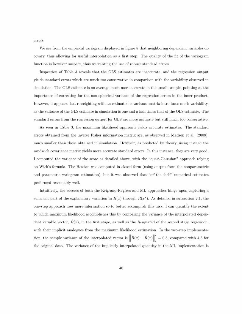
errors.
We see from the empirical variogram displayed in figure 8 that neighboring dependent variables do
covary, thus allowing for useful interpolation as a first step. The quality of the fit of the variogram
function is however suspect, thus warranting the use of robust standard errors.
Inspection of Table 3 reveals that the OLS estimates are inaccurate, and the regression output
yields standard errors which are much too conservative in comparison with the variability observed in
simulation. The GLS estimate is on average much more accurate in this small sample, pointing at the
importance of correcting for the non-spherical variance of the regression errors in the inner product.
However, it appears that reweighting with an estimated covariance matrix introduces much variability,
as the variance of the GLS estimate in simulation is one and a half times that of the OLS estimate. The
standard errors from the regression output for GLS are more accurate but still much too conservative.
As seen in Table 3, the maximum likelihood approach yields accurate estimates. The standard
errors obtained from the inverse Fisher information matrix are, as observed in Madsen et al. (2008),
much smaller than those obtained in simulation. However, as predicted by theory, using instead the
sandwich covariance matrix yields more accurate standard errors. In this instance, they are very good.
I computed the variance of the score as detailed above, with the “quasi-Gaussian” approach relying
on Wick’s formula. The Hessian was computed in closed form (using output from the nonparametric
and parametric variogram estimation), but it was observed that “o�-the-shelf” numerical estimates
performed reasonably well.
Intuitively, the success of both the Krig-and-Regress and ML approaches hinge upon capturing a
su�cient part of the explanatory variation in R(x) through R(xú). As detailed in subsection 2.1, the
one-step approach uses more information so to better accomplish this task. I can quantify the extent
to which maximum likelihood accomplishes this by comparing the variance of the interpolated depen-
dent variable vector, R(x), in the first stage, as well as the R-squared of the second stage regression,
with their implicit analogues from the maximum likelihood estimation. In the two-step implementa-
tion, the sample variance of the interpolated vector is...R(x) ≠ R(x)
...2
2
= 0.8, compared with 4.3 for
the original data. The variance of the implicitly interpolated quantity in the ML implementation is
40

Figure 9: Nonparametric estimates of variance and covariance for Y and Rú as a function of distance.
3...Y (x) ≠ Y (x)...
2
2
≠ ‡2
Á
4/—2
1
= 4.8, which suggests a much greater use of information,10 as well as
some overfitting. Analogously, the R-squared for the regression step of Krig-and-Regress was 0.09, and
the implicit R-squared for the ML implementation was 0.69, which is an order of magnitude greater.
Inspection of figure 9 makes tangible the identification strength of the robust approach. The pattern
in the bottom-left plot of ‡úY Rú against distance shows the (decaying) negative correlation between
(neighboring) Y (x) and Rú(xÕ). It suggests that we are capturing su�cient variation to confirm an
impact of Rú on Y through R and thus, heuristically speaking, the existence of a “significant” —. The
scale of — can be assessed by comparing the magnitudes of ‡úY Rú and ‡ú
Rú .
If — is obtained from the ratio of the covariance of Rú and Y with the variance of Rú, how is this
approach conceptually di�erent from the ordinary least-squares approach? The key di�erence is that
it is using the information that the covariance function of Rú with Y and the variance of Rú are the
same up to rescaling by —, and it estimates — and ◊ jointly.
10Note that this is di�erent from
... ˆ
R◊(x) ≠ ˆ
R◊(x)
...2
2, where
ˆ
R◊(x) is the best linear predictor for R(x) using the
maximum likelihood estimate for the covariance parameters, which does not account for the “variation in
ˆ
R” explained
by variation in Y .
41

Mean Sim. Strd Errors Reg. Output Strd Error CoverageOLS -0.44 0.045 0.080 0.98GLS -0.33 0.071 0.099 0.97MLE -0.39 0.049 0.032 0.75
QMLE -0.39 0.049 0.050 0.952-step BB -0.40 0.069 0.061 0.93
Robust -0.43 0.095 0.117 0.94
Table 3: Cross-validation output. The mean is the average over all simulation draws. The simulationstandard errors are the standard deviations of the simulation draws. The output standard errors areobtained from the inverse Hessian evaluated at the estimated value of the parameter for MLE, andfrom the sandwich formula using Wick’s formula to compute fourth moments for QMLE. For thetwo-step Bayesian bootstrap, the mean is the average posterior mean, the regression output standarderrors are given by the average over simulation runs of the posterior standard deviation. The coveragecorresponds to the fraction of times the confidence interval, computed with the output standard errorsof the current run of the simulation, covered -0.38.
7 Reanalysis of Maccini and Yang (2009)
This section reanalyzes the data set investigated in Maccini and Yang (2009). In that paper, the
authors estimate the e�ect of a rainfall shock in infancy on adult socio-economic outcomes such as
education or health. The paper merges a rainfall measurements data set with survey data, both of
which have geographically located observations. The data sets are misaligned, as can be seen from
figure 1, which plots the respective locations.
The authors do point out a host of potential issues arising from misalignment and convincingly
tackle them using linear regression methods. They use a two-stage least-squares approach which, in
principle, is easy to compute and produces standard errors that account for uncertainty in the first
stage. I compare their approach with the more principled methods developed herein. I find that their
general conclusions hold up, but that the analysis nevertheless benefits from the use of my methods as
they yield some statistically and economically significant changes in the value of parameter estimates.
7.1 Data Description
The data set for the regression is obtained by merging two, misaligned data sets. The first data set
contains rainfall measurements from measuring stations across Indonesia. The whole rainfall data spans
42
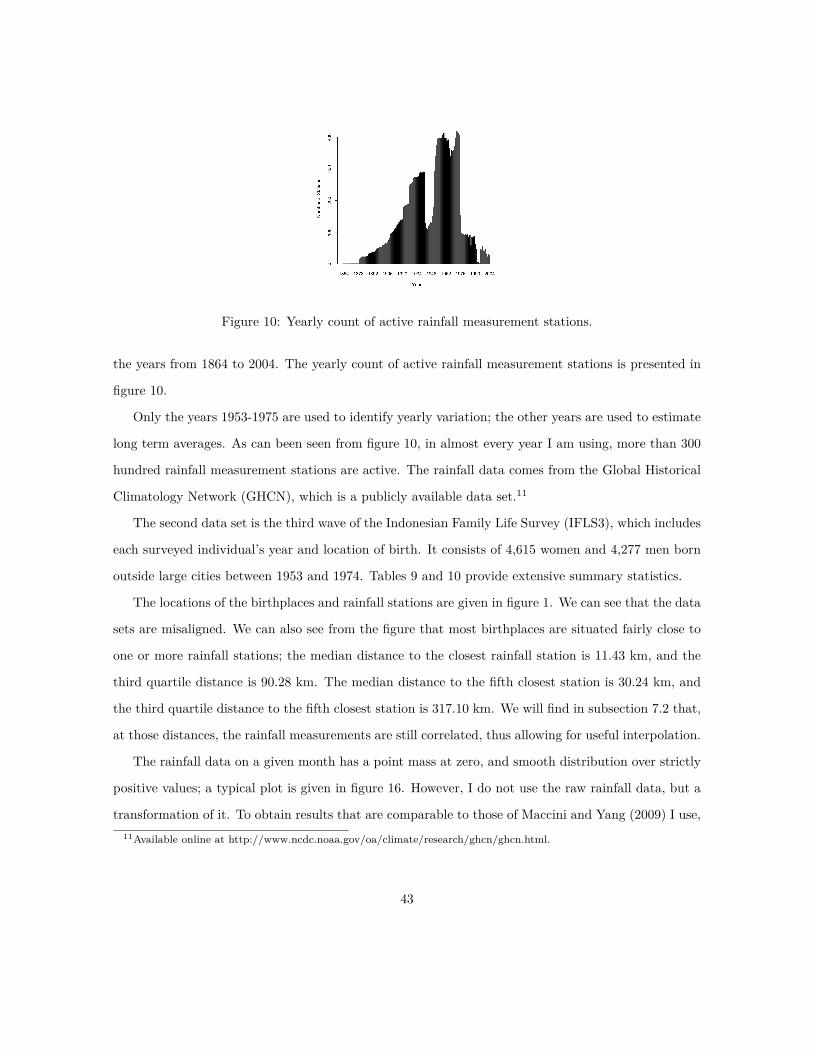
Figure 10: Yearly count of active rainfall measurement stations.
the years from 1864 to 2004. The yearly count of active rainfall measurement stations is presented in
figure 10.
Only the years 1953-1975 are used to identify yearly variation; the other years are used to estimate
long term averages. As can been seen from figure 10, in almost every year I am using, more than 300
hundred rainfall measurement stations are active. The rainfall data comes from the Global Historical
Climatology Network (GHCN), which is a publicly available data set.11
The second data set is the third wave of the Indonesian Family Life Survey (IFLS3), which includes
each surveyed individual’s year and location of birth. It consists of 4,615 women and 4,277 men born
outside large cities between 1953 and 1974. Tables 9 and 10 provide extensive summary statistics.
The locations of the birthplaces and rainfall stations are given in figure 1. We can see that the data
sets are misaligned. We can also see from the figure that most birthplaces are situated fairly close to
one or more rainfall stations; the median distance to the closest rainfall station is 11.43 km, and the
third quartile distance is 90.28 km. The median distance to the fifth closest station is 30.24 km, and
the third quartile distance to the fifth closest station is 317.10 km. We will find in subsection 7.2 that,
at those distances, the rainfall measurements are still correlated, thus allowing for useful interpolation.
The rainfall data on a given month has a point mass at zero, and smooth distribution over strictly
positive values; a typical plot is given in figure 16. However, I do not use the raw rainfall data, but a
transformation of it. To obtain results that are comparable to those of Maccini and Yang (2009) I use,11
Available online at http://www.ncdc.noaa.gov/oa/climate/research/ghcn/ghcn.html.
43
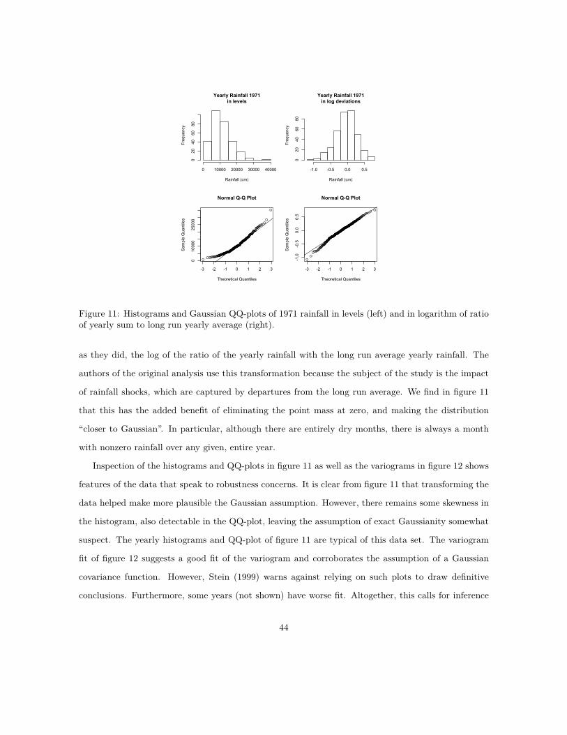
Yearly Rainfall 1971in levels
Rainfall (cm)Frequency
0 10000 20000 30000 40000
020
4060
80
Yearly Rainfall 1971in log deviations
Rainfall (cm)
Frequency
-1.0 -0.5 0.0 0.5
020
4060
80
-3 -2 -1 0 1 2 3
010000
25000
Normal Q-Q Plot
Theoretical Quantiles
Sam
ple
Qua
ntile
s
-3 -2 -1 0 1 2 3
-1.0
-0.5
0.0
0.5
Normal Q-Q Plot
Theoretical Quantiles
Sam
ple
Qua
ntile
s
Figure 11: Histograms and Gaussian QQ-plots of 1971 rainfall in levels (left) and in logarithm of ratioof yearly sum to long run yearly average (right).
as they did, the log of the ratio of the yearly rainfall with the long run average yearly rainfall. The
authors of the original analysis use this transformation because the subject of the study is the impact
of rainfall shocks, which are captured by departures from the long run average. We find in figure 11
that this has the added benefit of eliminating the point mass at zero, and making the distribution
“closer to Gaussian”. In particular, although there are entirely dry months, there is always a month
with nonzero rainfall over any given, entire year.
Inspection of the histograms and QQ-plots in figure 11 as well as the variograms in figure 12 shows
features of the data that speak to robustness concerns. It is clear from figure 11 that transforming the
data helped make more plausible the Gaussian assumption. However, there remains some skewness in
the histogram, also detectable in the QQ-plot, leaving the assumption of exact Gaussianity somewhat
suspect. The yearly histograms and QQ-plot of figure 11 are typical of this data set. The variogram
fit of figure 12 suggests a good fit of the variogram and corroborates the assumption of a Gaussian
covariance function. However, Stein (1999) warns against relying on such plots to draw definitive
conclusions. Furthermore, some years (not shown) have worse fit. Altogether, this calls for inference
44

Figure 12: Plots of empirical and fitted semivariogram using the exponential (black), Gaussian (blue)and linear (green) models. The data is from the year 1971.
with methods that are robust to covariance model misspecification.
7.2 Regression Analysis
The first order of business is to obtain a two-step estimator. I use the Krig-and-Regress method, which
is a consistent two-step method. It would be a natural first inclination to want to perform Kriging on
the monthly data, and then aggregate the monthly predictions over the year to obtain the transformed
data points. Indeed, we can see from figure 16 that on a typical year, the covariance functions are
quite di�erent for each month. I find however that Kriging on the log ratio of yearly rainfall to long
run yearly average is preferable. First, it seems to follow a well-behaved covariance function for which
I have twelve times more data; second, the transformed data seems closer to Gaussian, and has no
point mass at zero, as can be seen from figure 11; third, it makes more immediate the comparison with
the regression output of Maccini and Yang (2009) and with the QML output. Most importantly, if the
imputed covariate is a nonlinear transformation of the interpolated quantity, the estimated coe�cients
may not be consistent estimators of the best linear predictor coe�cients.
A potential concern is the isotropy assumption, i.e., that the direction of the vector giving the
di�erence between the locations of two points in the random field does not matter. That is, for the
variogram to only be a function of the distance between its arguments, and not the direction of the
vector from one to the other, we must assume that the direction does not impact the covariance. One
45
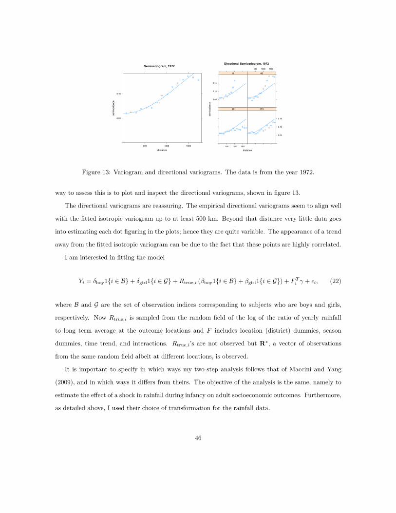
Semivariogram, 1972
distance
semivariance
0.05
0.10
500 1000 1500
Directional Semivariogram, 1972
distance
semivariance
0.05
0.10
0.15
0
500 1000 1500
45
500 1000 1500
90
0.05
0.10
0.15
135
Figure 13: Variogram and directional variograms. The data is from the year 1972.
way to assess this is to plot and inspect the directional variograms, shown in figure 13.
The directional variograms are reassuring. The empirical directional variograms seem to align well
with the fitted isotropic variogram up to at least 500 km. Beyond that distance very little data goes
into estimating each dot figuring in the plots; hence they are quite variable. The appearance of a trend
away from the fitted isotropic variogram can be due to the fact that these points are highly correlated.
I am interested in fitting the model
Yi = ”boy
1{i œ B} + ”girl
1{i œ G} + Rtrue,i (—
boy
1{i œ B} + —girl
1{i œ G}) + F Ti “ + ‘i, (22)
where B and G are the set of observation indices corresponding to subjects who are boys and girls,
respectively. Now Rtrue,i is sampled from the random field of the log of the ratio of yearly rainfall
to long term average at the outcome locations and F includes location (district) dummies, season
dummies, time trend, and interactions. Rtrue,i’s are not observed but Rú, a vector of observations
from the same random field albeit at di�erent locations, is observed.
It is important to specify in which ways my two-step analysis follows that of Maccini and Yang
(2009), and in which ways it di�ers from theirs. The objective of the analysis is the same, namely to
estimate the e�ect of a shock in rainfall during infancy on adult socioeconomic outcomes. Furthermore,
as detailed above, I used their choice of transformation for the rainfall data.
46
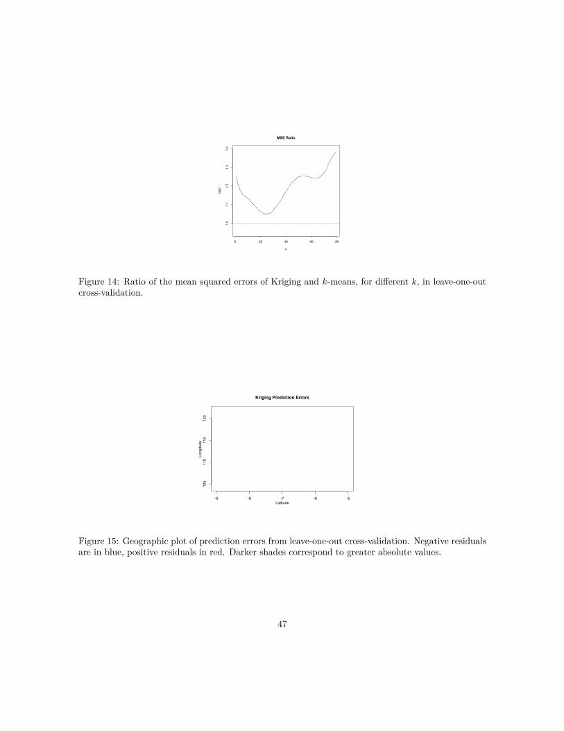
0 20 40 60 80
1.0
1.1
1.2
1.3
1.4
MSE Ratio
k
ratio
Figure 14: Ratio of the mean squared errors of Kriging and k-means, for di�erent k, in leave-one-outcross-validation.
-9 -8 -7 -6 -5
105
110
115
120
Kriging Prediction Errors
Latitude
Longitude
Figure 15: Geographic plot of prediction errors from leave-one-out cross-validation. Negative residualsare in blue, positive residuals in red. Darker shades correspond to greater absolute values.
47

I use a di�erent two-step method than Maccini and Yang (2009) did. Whilst I do the interpolation
step with the best linear predictor, they use an instrumental variables approach. Their strategy
is to estimate (22) by running a two-stage least-squares regression in which the nearest rainfall is
instrumented with slightly more distant rainfall stations (the second to fifth closest stations). This
approach is problematic for two reasons. Conceptually, there is no reason to believe that instrumenting
the wrong rainfall measurements with other wrong rainfall measurements will “wash away” the error
term which can be thought of as the di�erence between the rainfall at the outcome location and the
rainfall at the nearest station (for instance, all stations could be near each other and have correlated
“errors”). Practically, the data set at hand makes this strategy di�cult to implement; the missing
rainfall observations are many and sporadic such that, for any given outcome location, there will be
few years for which the nearest rainfall station and all of the next four nearest stations will have
observed measurements. Eliminating the incomplete observations reduces the data set substantially
and imputing, say, medians impacts the outcome tangibly.
A natural alternative, for purposes of interpolation, is k-means. I compare the performance of
k-means with with Kriging to justify the use of a more sophisticated method. Figure 14 displays the
ratio of mean squared errors in a leave-one-out cross-validation exercise using the rainfall data. We
see that there are benefits justifying the use of Kriging for interpolation; for all reasonable choices of
number of neighbors k, Kriging dominates k-means in terms of mean squared error.
To further assess the quality of the Kriging estimates, I plot the geographically located interpolation
errors from leave-one-out cross-validation in figure 15. It appears there is not much spatial correlation
left in the residuals.
The second stage for the Krig-and-Regress is done by ordinary least-squares. I found that using
feasible generalized least-squares did not help in this case. In particular, fitting a covariance function
to the regression errors is di�cult, and the fit needs to be quite good to tangibly ameliorate the point
estimates.
Implementation of the Krig-and-Regress approach yields results that are similar to those of Maccini
and Yang (2009).
To apply the QML approach to model (22), I need to accommodate an interaction term on the
48

regression coe�cient for rainfall. Observing, as in subsection 1.1, that the mean is overparametrized,
I can write the likelihood as
Q
caY
Rú
R
db ≥ NN+M
Q
ca
Q
caX’
mú
R
db ,
Q
ca�
11
�12
�21
�22
R
db
R
db , (23)
where X includes F as well as gender e�ects for boys and girls. The blocks of the covariance matrix
are
(�11
)ij = (—boy
1{i œ B} + —girl
1{i œ G}) (—boy
1{j œ B} + —girl
1{j œ G}) Kij + �ij ,
(�12
)ij = (—boy
1{i œ B} + —girl
1{i œ G}) Kij ,
�21
= �T12
and �22
= Kú,
where 1B = (1{i œ B})i is the vector of indicator for boys, and 1G = (1{i œ G})i is the vector of
indicator for girls.
The coe�cient of interest only figures in the covariance, and I obtain estimates using REML, which
is tantamount to maximizing the likelihood for
Q
caQY
Rú
R
db ≥ NN≠p+M
Q
ca
Q
ca0
mú
R
db ,
Q
caQ�
11
QT Q�12
�21
QT �22
R
db
R
db , (24)
where Q is a full rank (n ≠ rank(X)) ◊ n matrix satisfying QX = 0.
When maximizing the log-likelihood, I use the output of the Krig-and-Regress procedure as starting
values for the optimization algorithm.
As did Maccini and Yang (2009), I find that the e�ects are more pronounced for girls than for boys.
Table 4 gives the estimated coe�cients for five outcome variables considered in the original analysis.
I find, as they did, a significant e�ect of rainfall shocks on the indicator of self-reported very good
health. However, although they found rainfall shocks in infancy to have a significant impact on adult
height as well as on the indicator of self-reported poor health, these findings are not maintained when
using robust uncertainty assessments.
49

Point estimates appear to behave as suggested by the theory and simulations. As observed in
the cross-validation exercise of Madsen et al. (2008), the standard errors of the (assumed to be
well-specified) maximum likelihood output are much too narrow and may mislead the researcher into
concluding statistical significance when unwarranted. In all instances the standard errors increased
when using a covariance formula which is robust to covariance function misspecification.
As expected from the well-behaved histograms and QQ-plots of figure 11, nonparametric estimation
of the fourth-order moments did not alter the standard errors substantially, although they did increase
in some instances.
The comparison of the output for the Krig-and-Regress method and the Bayesian bootstrap method
is informative. In particular, the standard errors provided for the two-step Bayesian bootstrap do take
into account the uncertainty in the imputation of the missing covariate, while those provided in the
output of the Krig-and-Regress method do not. As ought to be expected, the standard errors for the
two-step Bayesian bootstrap are larger than for Krig-and-Regress.
The maximum likelihood point estimate is about 0.1 higher than that of the two-step method. This
means that the estimated impact of one standard deviation in yearly rainfall, away from the long term
average, on the probability of declaring oneself very healthy increases from 3.5% to 6.3%, which is a
di�erence of considerable economic magnitude.
All of Krig-and-Regress, robust estimator, and two-step Bayesian bootstrap provide point estimates
which can be compared to that of maximum likelihood to help assess its robustness to the specification
of a covariance function for the regression errors. One must exercise caution when carrying out such a
robustness check; the change in the value of the regression coe�cient estimate can be brought about
both by the gain in information from moving to a more e�cient method, and by misspecification of
the regression error covariance. The fact that the one-step estimate is within the confidence interval
of the robust estimate (for reasonable critical values) corroborates the former explanation.
Discussion of the specific sources of misspecification is warranted. Inspection of table 4 shows
that standard errors changed more when allowing for covariance function misspecification than for
distribution misspecification, leading one to suspect that the former misspecification issue is the most
important one. In a sense, it is the less preferred one as I have shown that with misspecified dis-
50

M&Y 2-step (K-R) 2-step (BB) ML QML (Wick) QML Robust(a) —
girl
0.101(0.058)
ú0.104(0.085)
0.107(0.094)
0.195(0.034)
úúú0.195
(0.061)
úú0.195
(0.063)
úú0.116(0.118)
—boy
≠0.029(0.072)
≠0.079(0.084)
≠0.079(0.094)
0.001(0.037)
0.001(0.062)
0.001(0.067)
≠0.149(0.126)
(b) —girl
≠0.192(0.082)
úú≠0.074(0.089)
≠0.070(0.101)
≠0.088(0.062)
≠0.088(0.103)
≠0.088(0.107)
≠0.131(0.195)
—boy
≠0.100(0.098)
0.013(0.083)
0.015(0.108)
0.001(0.063)
0.001(0.105)
0.001(0.110)
≠0.010(0.200)
(c) —girl
2.832(0.821)
úúú1.441(1.402)
1.333(1.637)
1.247(0.484)
úúú1.247(0.903)
1.247(0.942)
1.720(1.783)
—boy
0.998(1.795)
1.210(1.685)
1.010(2.010)
1.160(0.534)
ú1.160(0.935)
1.160(0.971)
1.517(1.930)
(d) —girl
≠1.175(0.831)
≠1.169(0.842)
≠1.232(0.972)
≠0.868(0.401)
ú≠0.868(0.632)
≠0.868(0.657)
≠1.225(1.150)
—boy
0.515(0.779)
≠0.761(1.020)
≠0.735(1.231)
≠0.011(0.443)
≠0.011(0.675)
≠0.011(0.683)
0.143(1.347)
(e) —girl
1.086(0.453)
úú0.392(1.035)
0.405(1.161)
0.414(0.472)
0.414(0.599)
0.414(0.625)
0.214(1.174)
—boy
≠0.474(1.490)
≠0.125(1.044)
≠0.140(1.184)
0.007(0.478)
0.007(0.615)
0.007(0.639)
≠0.005(1.201)
Table 4: E�ect of birth year rainfall on (a) indicator for very good self-reported health status; (b)indicator for poor or very poor self-reported health status; (c) adult height; (d) days absent dueto illness (on four weeks preceding survey); (e) completed grades of schooling. The Maccini andYang (M&Y) estimates are taken from the original paper; Krig-and-Regress (K-R) uses OLS in thesecond stage and the standard errors of the OLS output; the procedure for the two-step Bayesianbootstrap (BB) is as detailed in section 4, with the di�erence that additional covariates are added inthe second stage. The point estimate is the posterior mean. Maximum likelihood (ML) uses the inverseHessian (the Hessian is computed in closed form) to obtain the asymptotic variance. Quasi-maximumlikelihood with Wick’s formula (QML (Wick)) uses the sandwich formula for the asymptotic variancebut estimates the fourth-order moments using the Gaussian formula, and Quasi-maximum likelihood(QML) uses nonparametric estimates for fourth-order moments.
51

tributional assumptions but well specified first and second order moments, QMLE yields consistent
estimates. In fact, the large discrepancy between the standard errors obtained from the inverse Hessian
(ML) and those obtained from the sandwich formula using the Gaussian approximation to fourth-order
moments (QML (Wick)) suggests that the covariance function misspecification might be important.
However, the standard errors displayed the same behavior in table 3, in the cross-validation exercise,
but the point estimate was very accurate. This is perhaps not so surprising. In the spatial statistics
literature it has been shown that, under infill asymptotics, quite weak conditions su�ce to guarantee
that interpolation with the wrong covariance function will yield consistent and even e�cient estimates
of the interpolated variable (Stein (1988), Yakowitz and Szidarovsky (1985), Stein (1999)). Inquiring
into how this translates into good properties of estimates of — is an upcoming item on my research
agenda.
8 Discussion and Conclusion
The main purpose of this article was to modernize econometrics for spatial data, with a special fo-
cus on the case of misaligned data. As detailed in sections 1 and 2, one-step maximum likelihood
methods provide more e�cient estimators than two-step methods. However, the theory and computa-
tional methodology were lacking for robust inference using the maximum likelihood estimator. I have
provided asymptotic distribution theory for this estimator when the assumptions of Gaussianity and
well-specified covariance functions need to be relaxed. I have provided two empirical examples using
a quasi-maximum likelihood estimator for more e�cient inference.
I also developed methods for the case in which the researcher does not want to specify the covariance
structure of the regression errors, thus leaving the likelihood function for the full model unavailable.
First, I proposed a one-step minimum distance estimator and developed its limit distribution theory,
thus producing correct standard errors for the estimator. Second, I suggested a modified two-step
method which, by sampling the covariance coe�cient from its posterior distribution, produces credible
intervals that account for the variation due to the estimation of the imputed regressor. These are easy
to compute and have a frequentist interpretation. This contribution is important because, although
52
Krig-and-Regress is the commonly preferred method for two-step estimation in the misaligned data
regression problem, to the best of my knowledge the literature did not o�er standard errors which
account for estimation in the first stage without requiring specification of the regression error covariance
structure.
I would like to leave the reader with a clear sense of which method to use when. For regression
with misaligned data, if the researcher can posit a covariance structure for the regression errors, he
should use the maximum likelihood estimator. If the researcher is confident that both the covariance
functions and the Gaussianity are well specified, he should use the inverse Hessian as the formula for the
asymptotic variance. If the researcher believes only the covariance function specification is suspect,
then he should use the sandwich covariance formula and estimate the fourth-order moments with
Wick’s formula. If Gaussianity is also suspect, then the researcher should estimate the fourth-order
moments using the shrinkage estimator of subsection 3.2.2. A good robustness check is to compare the
point estimates to those of the minimum distance estimator and Krig-and-Regress. If the researcher
concludes that specification of the regression error covariance is too restrictive, he should use either
the minimum distance estimator or the Bayesian bootstrap two-step estimator. For both of these, I
provided standard errors which account for estimation of the covariance structure of the misaligned
variable. In economics, the e�ects estimated are often weak (e.g. impact of rainfall shocks during the
first year of life on adult health) and the more e�cient QML method ought to be preconized.
Estimation of fourth-order moments is an important topic for future research. I have suggested a
method, inspired from the statistical finance literature, to directly estimate the fourth-order moments.
More sophisticated (and di�cult to implement) estimation methods have been studied in the statistical
geology literature (Goodfellow et al. (2012), Dimitrakopoulos et al. (2010)). I believe, however, that
further research ought to focus on developing robust estimators which do not require the estimation of
fourth-order moments. Estimation in the spectral domain o�ers a promising line of inquiry. In recent
work, Rao (2015) produces limit distribution theory for the spatial periodogram under distribution
misspecification. The variance of the estimator then depends on fourth-order terms (through the tri-
spectra). A reasonable conjecture is that by smoothing the spatial periodogram, one could decrease
the fourth-order variance term enough to be comfortable ignoring it altogether, while introducing bias
53

su�ciently small that the point estimates would remain reliable.
Another fascinating line of research is the study of properties of the regression coe�cient when the
covariance function of the misaligned covariate is misspecified. Under infill asymptotics and assuming
only weak conditions, the interpolated variable is consistent and even e�cient. This certainly guar-
antees consistency of the regression coe�cient estimator, and perhaps e�ciency. It will be important
to assess the properties of the regression coe�cient estimates under increasing domain asymptotics
when the covariance function is misspecified, as this asymptotic framework seems to better describe
the situations that economists typically face when dealing with misaligned data.
In conclusion, I have provided e�cient and robust estimators for regression analysis with misaligned
data, which is an important problem in spatial econometrics. I have developed general limit distribution
theory where it was lacking, and I carried out a detailed reanalysis of a misaligned data set, where
it appeared that the methods I recommend were indeed required. I believe this article will serve as
a useful reference for applied economists carrying out regression analysis with misaligned data, and a
good starting point for more theoretically inclined econometricians who need to develop further results
for this problem.
Appendix
A.1 Mixing Assumptions and Distribution Theory
In this subsection, I detail and discuss the assumption on spatial dependence required for the limit dis-
tribution theory and give the postponed proofs for the limit distribution theory of the quasi-maximum
likelihood estimator with dependent data.
A.1.1 Mixing Assumptions
The distribution theory relies on the assumption that random variables “far enough” from each other
are approximately independent. Useful measures to quantify such concepts of limiting independence
can be borrowed from the theory of mixing random variables (Doukhan (1994), White (1984), Davidson
(1994), Billingsley (1995)).
54

For our purposes, the natural assumption is in term of spatial dependence.
I introduce some terminology (Doukhan (1994), Davidson (1994)). Given a probability space
(�, F , P ), let G and H be ‡-subfields of F , then the strong mixing coe�cient is defined
–(G, H) = supGœG,HœH
|P (G fl H) ≠ P (G) P (H)| .
Given some distance12 function d : D æ R+
, D µ R2, I define
–Y (k; u, v) = sup {–Y (G, H) ; d(G, H) Ø k, |G| Æ u, |H| Æ v} ,
for all G, H µ D and u, v > 0, where | · | denotes the area, d(A, B) = min {d(a, b) : a œ A, b œ B}, and
–Y (G, H) = – (XG, XH) ,
where XF is the ‡-algebra generated by YF = {Yx : x œ F}, F µ D . See Bradley (1989, 1993) for a
discussion of the importance of the bound on G and H in the definition of –Y .
We say that the random field Y is strongly mixing (or –-mixing) if
limkæŒ
–Y (k; u, v) = 0,
for all integers u, v Ø 0. I also define mixing sequences. If the random variables are indexed by an
ordered set T , then another notion of mixing is defined for the random sequence X = {Xt}tœT . Let
–X,k;u,v = sup {–X (G, H)} where the supremum is over G and H with |G| Æ u, |H| Æ v, and g < h≠k
for g œ G and h œ H. The process X is said to be strongly mixing (–-mixing) if
limkæŒ
–X,k;u,v = 0
for all u, v > 0.
In both cases, we say that the process is mixing of size ≠Ï if –m = O (–≠Ï≠Ám ) for some Á > 0.
12For our purposes, it will be a Euclidian or geodesic distance.
55
Although the spatial nature of our motivating analysis makes more natural and verifiable mixing
assumptions on the random field, the proof technique calls for mixing assumptions on sequences.
Fortunately, for any relabeling of YT = (Y (t1
), ..., Y (tn))Õ as YS = (Y1
, ..., Yn), treated as a mixing
sequence, we have that as long as the distance between any two sites is bounded below, it obtains that
limkæŒ –YT (k; u, v) = 0 implies limkæŒ –YS ,k;u,v = 0, for all u, v > 0. Hence, this is accommodated
by the increasing domain asymptotic set-up, which specifies precisely such a lower bound.
I comment on the implication of the strong mixing assumption in the case in which the data
generating process is in fact Gaussian. Piterbarg (2012) briefly explores the question, whilst Ibragimov
and Rozanov (2012) investigate the topic more thoroughly. An unfortunate fact is that one cannot
conveniently specify a su�cient condition for strong mixing in terms of the covariance of the process;
short of assuming its zeroing from some moment on, one can impose any conditions on the limiting
rate of decrease of the covariance, and it will always be possible to find a Gaussian stationary process
with this rate of decrease of its covariance, but which is not strongly mixing.
The problem is that the condition of strong mixing requires the appearance of almost all frequencies
in the spectrum, so that the process “is similar to” white noise. See also Kolmogorov and Rozanov
(1960) and Ibragimov (1971) for further discussion.
Piterbarg (2012) endeavors to rehabilitate the mixing condition for Gaussian processes by showing
that by discretizing the Gaussian process at any level of precision, a fast enough decreasing of the
correlation will imply strong mixing of the discretized process. For our purposes, this is innocuous,
because we can comfortably treat weather shocks at very far distances (e.g. Boston vs Hong Kong) as
independent.
A.1.2 Distribution Theory for QMLE
Let Xn,i = aii
!Z2
i ≠ E#Z2
i
$"+ 2
qj<i aij (ZiZj ≠ E [ZiZj ]) and Fn,i = ‡ (Zn1
, ..., Zn,i) , 1 Æ i Æ kn.
Suppose Zi is –-mixing of size ≠Ï. Further suppose that..Z2
i
..4
< Œ. I give the proof of Theorem 2.
Proof of Lemma 2
First, E [Xn,i| Fn,i+m] = Xn,i, and thus ÎXn,i ≠ E [Xn,i| Fn,i+m]Î2
= 0.
Second, observe that
56

ÎE [Xn,i| Fn,i≠m]Î2
Æ aii
..E#Z2
i
-- Fn,i≠m
$ ≠ E#Z2
i
$..2
+ 2ÿ
j<i
aij ÎE [ZiZj | Fn,i≠m] ≠ E [ZiZj ]Î2
.
I can bound each summand using moment inequalities for mixing variables. Note that the Z2
i ’s are
likewise –-mixing of size ≠Ï. From (Davidson, 1994, theorem 14.2), I have that
..E#Z2
i
-- Fn,i≠m
$ ≠ E#Z2
i
$..2
Æ 6–1/2
m
..Z2
i
..2
.
A bound for ÎE [ZiZj | Fn,i≠m]Î2
obtains either when Fn,i≠m contains little information about both i
and j, and when i and j are far apart. Let mÕ = Âm/2Ê. The first case is j ≠ i + m Ø mÕ. That is,
both i and j are greater than the indices of the random variables generating Fn,i≠m by at least mÕ.
Let k = i ≠ j, then ZiZj = ZiZi≠k is likewise –-mixing of size ≠Ï. Since Fi≠m ∏ Fi≠mÕ , I obtain
ÎE [ZiZj | Fn,i≠m] ≠ E [ZiZj ]Î2
2
= ÎE [E [ZiZj | Fn,i≠mÕ ]| Fn,i≠m] ≠ E [ZiZj ]Î2
2
= ÎE [E [ZiZj | Fn,i≠mÕ ] ≠ E [ZiZj ]| Fn,i≠m]Î2
2
Æ EËE
Ë(E [ZiZj | Fn,i≠mÕ ] ≠ E [ZiZj ])2
--- Fn,i≠m
ÈÈ
= EË(E [ZiZj | Fn,i≠mÕ ] ≠ E [ZiZj ])2
È
Æ1
6–1/2
mÕ ÎZiZjÎ2
22
Æ1
6–1/2
mÕ ÎZiÎ4
ÎZjÎ4
22
.
In the second case, when j ≠ i + m < mÕ, or equivalently i ≠ j > mÕ, it is the weak dependence of Zi
with Zj which allows to control the norm . Indeed, observe that
57
ÎE [ZiZj | Fn,i≠m] ≠ E [ZiZj ]Î2
2
= ÎE [E [ZiZj | Fn,i≠mÕ ]| Fn,i≠m] ≠ E [ZiZj ]Î2
2
= ÎE [E [Zi| Fn,i≠mÕ ] Zj ≠ E [ZiZj ]| Fn,i≠m]Î
Æ EËE
Ë(E [Zi| Fn,i≠mÕ ] Zj ≠ E [ZiZj ])2
--- Fn,i≠m
ÈÈ
= EË(E [Zi| Fn,i≠mÕ ] Zj ≠ E [ZiZj ])2
È
Æ1
2(23/4 + 1)–1/2
mÕ ÎZiÎ4
ÎZjÎ4
22
,
using the covariance inequality for mixing sequences. Thus
ÎE [ZiZj | Fn,i≠m] ≠ E [ZiZj ]Î2
Æ 6–1/2
mÕ ÎZiÎ2
4
always. Consequently,
ÎE [Xn,i| Fn,i≠m]Î2
Æ aii6–1/2
m
..Z2
i
..2
+ÿ
j<i
aij6–1/2
mÕ ÎZiÎ2
4
. –1/2
m ÎZiÎ2
4
ÿ
jÆi
aij
Æ –1/2
m iM = O(m≠1/2),
where M is an implicitly defined constant in m. In particular, an,i = iM are the mixingale magnitude
indices. ⇤
I move onto the central limit theorem for quadratic forms in mixing random variables. I obtain a general
result showing that, upon conditions on the sequences of matrices {An}, a CLT for the quadratic forms
ZTn AnZn obtains.
For each n, let Xn1
, ..., Xnkn be independent with mean 0 and normalized to have variance 1. The
proof of the mixingale central limit theorem relies on a Bernstein blocks strategy. The idea is to divide
58
the data into large and small blocks, with a small block separating every two consecutive large blocks,
so to treat the sum of entries within each large block as (asymptotically) independent observations.
Let an and bn be the sizes of the big and small blocks, respectively. Define big blocks
‰ns =sbnÿ
i=(s≠1)(bn+ln)+1
Xni, s = 1, ..., rn,
where rn =Í
nbn+ln
Î. I define the asymptotic framework such that bn/ln æ Œ, ln/n æ 0, bn/n æ 0,
and that b2
n/n is bounded in probability.
This corresponds to a pure increasing domain asymptotic framework for the underlying spatial
data. In applications to merged data, the sample size of both data sets must go to infinity for the
conclusions of this theory to carry through.
The mixingale central limit theorem requires conditions on extremum statistics. For mixingale
magnitude indices ani, define
Mns = max(s≠1)(bn+ln)+1ÆiÆsbn
ani,
the maximum magnitude index for big block s.
Technical conditions are imposed in terms of expectations taken in the bulk and tails of the under-
lying data generating process. Define
”(1)
ni = E(X2
ni ≠ 1)21{|Xni|>Lni}, ”(2)
nij = E(X2
ni ≠ 1) (XniXnj ≠ µnij) 1{|Xni|>Lni},
”(3)
nij = E!X2
ni ≠ 1" !
X2
nj ≠ 1"
1{|Xni|>L,|Xnj |>Lni}},
where µnij = E[XiXj ] ’ i, j, and
”nij =
Y_]
_[
”(1)
ni , if i = j
”(2)
nij + ”(3)
nij , if i ”= j.
Define also
59
“(1)
nij = E(X2
ni ≠ 1)2(X2
nj ≠ 1)21{|Xnd| Æ Lnd, d = i, j},
“(2)
niljs = E(X2
ni ≠ 1)(X2
nj ≠ 1)(XniXnl ≠ µnil)(XnjXnl ≠ µnjl)1{|Xnd| Æ Lnd, d = i, j, l, s},
“(3)
niljsrt = E(XniXnl≠µnil)(XniXnr≠µnir)(XnjXns≠µnjs)(XnjXnt≠µnjt)1{|Xnd| > Lnd, d = i, l, j, s, r, }.
Theorem 3 Suppose that Zn1
, ..., Znkn are –-mixing of size 1, and let Xn1
, ..., Xnkn and Fn1
, ..., Fnkn
be defined as in (15) and (16), respectively. Assume that An, n = 1, 2, ..., is symmetric and
that all fourth-order products ZniZnjZnkZnl are uniformly integrable. Assume that there are
numbers {Lni}1ÆiÆkn,nØ1
such that
1‡2
n
knÿ
i,j
a2
nij”nij æ 0 (25)
1‡2
n
knÿ
i=1
Q
aknÿ
j=1
a(1)
nij“(1)
nij +knÿ
iÕ=1
ÿ
j ”=i,jÕ ”=iÕ
Q
aa(2)
nijls“(2)
nijls +ÿ
r ”=i,t”=j
a(3)
niljsrt“(3)
niljsrt
R
b
R
b æ 0, (26)
where a(1)
nij = a2
niia2
njj , a(2)
nijls = aniianjjanilanjs, a(3)
niljsrt = anilanjsanjranjt and ‡2
n = V ar(X Tn AnXn)
with X Tn = (Xn1
, ..., Xnkn). Further assume that
⁄max
1!A0
n
"2
2
‡2
n
æ 0, (27)
where A0
n is equal to An with the diagonal terms replaced by zeros. Then
X Tn AnXn ≠ EX T
n AnXn
‡n
L2æ N(0, 1). (28)
Proof
By lemma 2, I know that {Xni, Fni} is an L2
mixingale of size ≠1/2. Let ani, i = 1, ..., kn denote its
mixingale magnitude indices. In order to establish (29), it su�ces to show that Xn1
, ..., Xnkn satisfies
the conditions of De Jong (1997), Theorem 1.
The distance between any two points Zni, and thus their dependence, is bounded. The dependence
60
vanishes as the distance between the location corresponding to two points Zni and Znj gets bigger (or,
eventually, as the di�erence in their indices gets arbitrarily large). Thus I know that the mixingale
magnitude indices are bounded in n and i. In particular, from the condition on the relative size of big
blocks, bn/n æ 0, I know that n≠1/2/b≠1/2 æ 0, which gives ani/b≠1/2
n æ 0. Likewise, rnb2
n
n2b≠1
n= O(1)
must be bounded, and thusqrn
s=1
M2
ns = O(b≠1
n ). By uniform integrability of the fourth-order products
of Zni’s, I know that X2
ni/a2
ni is uniformly integrable.
Write
X Tn AnXn ≠ EX T
n AnXn
‡n=
knÿ
i=1
›ni +knÿ
i=1
÷ni
where
›ni = 1‡n
Q
aaniiUni + 2
Q
aÿ
j<i
anijUnij
R
b
R
b ,
÷ni = 1‡n
Q
aaniiVni + 2
Q
aÿ
j<i
anijVnij
R
b
R
b ,
with
Uni =!X2
ni ≠ 1"
1{|Xni|ÆLni} ≠ E!X2
ni ≠ 1"
1{|Xni|ÆLni}, Vni = X2
ni ≠ 1 ≠ Uni,
Unij = (XniXnj ≠ µnij) 1{|Xnd|ÆLnd,d=i,j}≠E (XniXnj ≠ µnij) 1{|Xnd|ÆLnd,d=i,j}, Vnij = XniXnj≠µnij≠Unij .
By (1), I have thatqkn
i=1
÷iL
2æ 0. Note that the statements for the mixingale magnitude indices of
the untruncated mixingale hold for those of the truncated mixingale. Hence, it su�ces to show that
the array of mixingales ›ni satisfy the mixingale central limit theorem. That is, it su�ces to establish
that condition (12) from De Jong (1997) Theorem 1, is satisfied. This requires showing that the sum
of the squared sums over big Bernstein blocks is 1, i.e.
rnÿ
s=1
X 2
nsPæ 1.
61
Note thatqrn
s=1
1qsbn
i=(s≠1)bn+ln+1
›2
ni
2=
1qkn
i=1
›ni
22
≠ qi⌧j ›ni›nj , where i ⌧ j means that the ith
and jth observations are not in the same big Bernstein block. By the mixing condition, and because
bn æ Œ, I can establish thatq
i⌧j ›ni›nj = op(1). Consider
ÿ
i⌧j
›ni›nj = 1‡2
n
ÿ
i⌧j
AaniiUni + 2
Aÿ
l<i
anilUnil
BB Q
aanjjUnj + 2
Q
aÿ
s<j
anjsUnjs
R
b
R
b
= 1‡2
n
ÿ
i⌧j
Q
aaniianjjUniUnj + 2A
ÿ
l<i
anilUnil
BanjjUnj + 2
Q
aÿ
s<j
anjsUnjs
R
b aniiUni + 4A
ÿ
l<i
anilUnil
B Q
aÿ
s<j
anjsUnjs
R
b
R
b
= 4‡2
n
ÿ
i⌧j
Aÿ
l<i
anilUnil
B Q
aÿ
s<j
anjsUnjs
R
b + op(1)
= 4‡2
n
ÿ
i⌧j
1BT
(i)U(i)
2 1BT
(j)
U(j)
2
= 4‡2
n
ÿ
i⌧j
UT(i)B
T(i)B(j)
U(j)
= 4‡2
n
UT A0
U
where B(l) =
!anil1{l<i}
"i, , B = (BT
(1)
, ..., , BT(k)
)T , U(l) = (Unil)i, U =
!U
(1)
, ..., U(k)
". Note that
A0
= vec(B)vec(B)T ≠ (I ¢ vec(B))(I ¢ vec(B))T ,
where the second term removes the block-diagonal corresponding to entries in the same big Bernstein
block. Now note that1
‡4
n
E!UT A
0
U"
2
= 1‡4
n
E
Q
ak2
nÿ
i,j=1
A0ijUiUj
R
b2
62

Æ 2c1
‡4
n
Q
ak2
nÿ
i,j=1
A2
0ijE!U2
i U2
j
"R
b (29)
Æ 2c2
‡2
n
..A0
..2
FÆ ⁄
max
!A
0
"
‡2
n
Æ 1‡2
n
maxi,s
Y__]
__[|anis| ·
ÿ
j⌧il<j
|ajl|
Z__
__\+ op(1) (30)
Æ 1‡2
n
ÎBÎ2
F
Æ c3
‡2
n
⁄max
!BBT
"
Æ c4
‡2
n
1tr
1!BT B
"2
221/2
Æ c5
A⁄
max
!(A
0
)2
"
‡2
n
B1/2
tr (BT B)
‡n(31)
where (30) follows from Rosenthal’s inequality, (31) from Gersgorin’s circle theorem, and (32) from
lemma 5.1 of Jiang (1996). Then, since ⁄max
((A0
)
2)‡2
næ 0, I have that
qi⌧j ›ni›nj æ 0.
Therefore it su�ces to show that Aknÿ
i=1
›ni
B2
Pæ 1.
Write
Aknÿ
i=1
›ni
B2
=knÿ
i,j=1
›ni›nj =3ÿ
i=i
Ui +3ÿ
i=i
Vi
where
63

U1
= 1‡2
n
knÿ
i,j=1
aniianjj (UniUnj ≠ EUniUnj) ,
U2
= 2‡2
n
knÿ
i,j=1
anii
Q
aÿ
s<j
anjsUniUnjs ≠ E
Q
aÿ
s<j
anjsUniUnjs
R
b
R
b ,
U3
= 4‡2
n
knÿ
i,j=1
Q
ca
Aÿ
l<i
anilUnil
B2
≠ E
Q
aÿ
s<j
anjsUnjs
R
b2
R
db ,
V1
= 1‡2
n
knÿ
i=1
aniianjjEUniUnj ,
V2
= 2‡2
n
knÿ
i,j=1
aniiE
Q
aÿ
s<j
anjsUniUnjs
R
b
V3
= 4‡2
n
knÿ
i,j=1
E
Q
aÿ
s<j
anjsUnjs
R
b2
.
By (27) I have that UiL
2æ 0 for i = 1, 2, 3. By (26) I then have that
V1
= 1‡2
n
knÿ
i,j=1
aniianjjCov(X2
ni, X2
nj) + op(1),
V2
= 2‡2
n
knÿ
i,j=1
ÿ
s<j
aniianjsCov!XnjXns, X2
ni
"+ op(1),
V3
= 4‡2
n
knÿ
i,j=1
ÿ
l<i
ÿ
s<j
anijanijÕCov(XniXnl, XnjXns) + op(1)
Thus I have that
rnÿ
s=1
X 2
ns =q
ijiÕjÕ anijaniÕjÕCov (XnjXni, XnjÕXniÕ) + op(1)‡2
n
Pæ 1.
64

⇤
Remark The conditions of theorem 3 reduce to the conditions of theorem 5.2 of Jiang (1996) in the
case of independent random variables.
Remark Note that the argument of Jiang (1996), theorem 5.1 applies here, and conditions (26), (27)
and (28) can be replaced with
infn
(mini
V ar(Xni)) · ( mini:aii ”=0
V ar(X2
ni)) > 0,
supn
( max1ÆiÆn
EX2
ni1{|Xni|>x}) ‚ ( maxi:aii ”=0
EX4
ni1{|Xni|>x}) æ 0,
as x æ 0, and⁄
max
1(A
0
)2
2
‡2
n
æ 0,
for a proper choice of Ln.
A1.3 Distribution Theory for Robust Estimation
To keep with the literature on asymptotics for semivariograms, I denote the mixing coe�cients slightly
di�erently in this subsection. Define
–(a; b) = sup {–(T1
, T2
) : d(T1
, T2
) Ø a, T1
, T2
œ S3
(b)} ,
where S3
(b) =Ót
3
i=1
Di :q
3
i=1
|Di| Æ bÔ
is the collection of all disjoint unions of three cubes D1
, D2
, D3
in R2, –(T1
, T2
) = sup {|P (A fl B) ≠ P (A)P (B)| : A œ ‡ ÈR(s)|s œ T1
Í , B œ ‡ ÈR(s)|s œ T2
Í}, and d(T1
, T2
) =
min {Îx1
≠ x2
Î : x1
œ T1
, x2
œ T2
}.
To simplify the exposition, following Lahiri (2003), I further assume that there exist a non-increasing
function –1
(·) with limaæŒ –1
(a) = 0 and a nondecreasing function g(·) such that the strong-mixing
coe�cients –(a, b) satisfy
–(a, b) Æ –1
(a)g(b), a > 0, b > 0.
65

In order to obtain a central limit theorem for the minimum distance estimator, I must first obtain
a central limit theorem for the statistics from which I want to minimize distance. The following lemma
is a useful preliminary result.
Lemma A.1 Let {Y (s) : s œ Rd} be a stationary random field with EY (0) = 0 and autocovariance
function ‡(s) = EY (0)Y (s), s œ Rd. Suppose E |Y (0)|2+” < Œ for some ” > 0. Suppose f is
strictly greater than 0 and continuous on R0
. Assume that –(a, b) Æ Ca≠3 log(a)g(b) , a, b > 1,
for a bounded g. Then for n/⁄2
n æ C1
,
n≠1/2
nÿ
i=1
Y (si)dæ N
30, ‡(0) + Q · C
1
·ˆRd
‡(x)dx
4,
almost surely, where Q =´
f2(x)dx and ‡(x) = EY (0)Y (x).
Proof of Lemma A.1
The claim follows directly from Proposition 3.1 and Theorem 3.2 of Lahiri (2003). ⇤
I can now give the central limit theorem for the objective function of the robust estimation opti-
mization problem.
A key observation is that even while maintaining the pure-increasing asymptotic framework for
stochastic designs (as opposed to positing one in which the observations also get denser), the bins
of the nonparametric semivariogram, Nn(·), can both shrink and contain more observations as we
move along the sequence in n. The set of pairs of observations which will be used to approximate the
semivariogram evaluated at a certain distance d, the “bin”, is defined by the lower and upper bounds
on the distance, b and b. The nonparametric variogram is
gn(d) = 1|Nn(d)|
ÿ
(i,j)œNn(d)
(R(xi) ≠ R(xj))2,
and the bins Nn(d) used to estimate the squared di�erence of pairs distance d apart, with sample size
n, are defined
66

Nn(d) =)
(si, sj) : 1 Æ i, j Æ n, bn(d) Æ d(si ≠ sj) Æ bn(d)*
.
It is assumed that bn(d), bn(d) æ d, pointwise. Furthermore, it is assumed that |Nn(h)| = O(n).
Remark I prove a more general result than stated in the main body of the article. Let the mean of the
random field be x(s)T fl instead of the constant m, and replace the assumption ⁄2
n Îm ≠ mÎ4
2
=
op(1) by sup {Îx(s) ≠ x(s + h)Î : s œ R} Æ C(h) < Œ and ⁄2
n Îfl ≠ flÎ4
2
= op(1).
Proof of Theorem 6
Using the Cramér-Wold device, it su�ces to show that n1/2aT g(„0
) dæ N!0, aT �g(„
0
)a"
as n æ Œfor any a œ RK . Let
g1n = n1/2
Kÿ
k=1
ak
Q
a 1|Nn(hk)|
ÿ
Nn(hk)
(R(si) ≠ R(sj))2 ≠ 2“(hk; ◊0
)
R
b ,
and
g2n = n1/2
Kÿ
k=1
ak
A1n
nÿ
i=1
(R(si) ≠ R(si + hk))2 ≠ 2“(hk; ◊0
)B
.
The strategy is to show that gn is close to g1n, which is close to g
2n, which satisfies the conditions
of the central limit theorem obtained in Lemma A.1. Note that
|g1n ≠ gn| Æ n1/2
Kÿ
k=1
|ak||Nn(hk)|
ÿ
Nn(hk)
----1
R(si) ≠ R(sj)2
2
≠ (R(si) ≠ R(sj))2
----
n1/2
Kÿ
k=1
|ak||Nn(hk)|
ÿ
Nn(hk)
---((fl ≠ fl) (x(si) ≠ x(xj)) ≠ (R(si) ≠ R(sj)))2 ≠ (R(si) ≠ R(sj))2
---
Æ C1
n1/2
Kÿ
k=1
|ak|1
Îfl ≠ flÎ2
2
C(bn(hk))2 + 2 Îfl ≠ flÎ2
ÎEk,nÎ2
2
where Ekn =q
Nn(hk)
1
|Nn(hk)| (x(si) ≠ x(sj)) (R(si) ≠ R(sj)) = O(n≠1). Then under increasing-
domain asymptotics and since E Îfl ≠ flÎ2
2
= O(⁄≠1
n ), I obtain that |g1n ≠ gn| = op(1).
67

Since ⁄n æ Œ and f > a > 0, I know that |Jkn| =´
Jknf(x)dx æ 0 where Jkn = R
0
\ (1 ≠ hk,n/⁄n) R0
,
for k = 1, ..., K, and therefore |Nn(hk)| = n (1 + o(1)). Consequently, by mean square continuity, it
follows that
E |g1n ≠ g
2n| Æ C2
E
------n1/2
Kÿ
k=1
ak
Q
aÿ
(i,j)œNn(hk)
1|Nn(hk)| (R(si) ≠ R(sj))2 ≠ 1
n
nÿ
i=1
(R(si) ≠ R(si + hk))2
R
b
------
Æ C2
E
------n1/2
Kÿ
k=1
ak
Q
aÿ
(i,j)œNn(hk)
1|Nn(hk)| (R(si) ≠ R(sj))2 ≠ 1
n
ÿ
i:(i,j)œNn(hk)
(R(si) ≠ R(si + hk))2
R
b
------
+C2
E
------n1/2
Kÿ
k=1
ak1n
ÿ
i:(i,j)/œNn(hk)
(R(si) ≠ R(si + hk))2
------
Æ C2
n1/2
Kÿ
k=1
|ak|Q
a----
1|Nn(hk)| ≠ 1
n
---- E
Q
aÿ
(i,j)œNn(hk)
(R(si) ≠ R(si + hk))2
R
b
R
b
+C2
n1/2
Kÿ
k=1
|ak| 1n
E
Q
aÿ
i:(i,j)/œNn(hk)
(R(si) ≠ R(si + hk))2
R
b + op(1)
by mean square continuity of E1
(R(s) ≠ R(sÕ))2
2, and is
Æ C3
n1/2
Kÿ
k=1
|ak|A
||Nn(hk)| ≠ n| n≠2E
Anÿ
i=1
(R(si) ≠ R(si + hk))2
BB
+C3
n1/2
Kÿ
k=1
|ak| 1n
Q
caE
Q
aÿ
i:(i,j)/œNn(hk)
(R(si) ≠ R(si + hk))2
R
b2
R
db
1/2
Æ C4
n1/2
Kÿ
k=1
|ak|
Q
ca||Nn(hk)| ≠ n| n≠2
Q
aE
Anÿ
i=1
(R(si) ≠ R(si + hk))2
B2
R
b1/2
R
db
68

+C5
n1/2
Kÿ
k=1
|ak| 1n
Q
aÿ
i:(i,j)/œNn(hk)
Cov
Anÿ
i=1
(R(si) ≠ R(si + hk))2 , (R(0) ≠ R(0 + hk))2
BR
b1/2
Æ CKÿ
k=1
|ak|1
n≠1 ||Nn(hk)| ≠ n| + |Jnk|1/2 n≠1/2
2
which goes to 0, as n æ Œ.
Then it su�ces to show that g2n æ N(0, aT �g(„
0
)a), which follows from an application of Lemma
A.1. ⇤
With the asymptotic distribution of the statistic gn in hand, I can call on Theorem 3.2 of Cressie
and Lahiri (2002) and obtain Theorem 7 as an immediate corollary. I record the additional necessary
assumptions under Assumption 1.
Assumption A.1 Suppose that
• For any ‘ > 0, there exists ” > 0 such that infÓqK
i=1
(2“(hi; „1
) ≠ 2“(hi; „2
))2 : ΄1
≠ „2
Î Ø ‘Ô
>
”,
• sup)
“(h; „) : h œ R2, „ œ �*
< Œ, “(h; „) is continuously di�erentiable with respect to each
entry of „.
• W („) is positive definite for all „ œ � and sup)ÎW („)Î +
..W („)≠1
.. : „ œ �*
< Œ, and W („)
is continuously di�erentiable with respect to each entry of „.
A1.4 Proof of Theorem 5
I give the proof of Theorem 5.
Proof of theorem 5
First observe that, by simple di�erentiation, I get
69
ˆ4
ˆ⁄1
...ˆ⁄4
EËÈ⁄, Y Í4
È= ˆ3
ˆ⁄2
...ˆ⁄4
E
S
U ˆ
ˆ⁄1
ÿ
1Æi,j,k,lÆ4
⁄i⁄j⁄k⁄lYiYjYkYl
T
V
= ˆ3
ˆ⁄2
...ˆ⁄4
E
S
U4Y1
ÿ
1Æj,k,lÆ4
⁄i⁄j⁄k⁄lYjYkYl
T
V
= · · ·
= 4!E [Y1
Y2
Y3
Y4
] ,
where ⁄ = (⁄1
, ..., ⁄4
). I obtain the identity
E [Y1
Y2
Y3
Y4
] = 14!
ˆ4
ˆ⁄1
...ˆ⁄4
EËÈ⁄, Y Í4
È. (32)
By Pinsker’s inequality, I know that DT V (F, P ) ÆÒ
1
2
b, where b = DKL(F ||P ). Note that total
variation can be expressed as
DT V (F, P ) = 12 sup
|h|Æ1
----ˆ
hdP ≠ˆ
hdF
---- ,
where h : Rn æ R.
In order to apply the bound on EËÈ⁄, Y Í4
È, I separate the integrand into a bounded function and
a remainder whose integral is negligible:
EËÈ⁄, Y Í4
È= E
ËÈ⁄, Y Í4 1{È⁄, Y Í4 Æ T}
È+ E
ËÈ⁄, Y Í4 1{È⁄, Y Í4 > T}
È
Since X is Gaussian and Y is sub-Gaussian, È⁄, XÍ4 are È⁄, Y Í4 are both ‹-subgaussian for some
‹. Then I have that
---EËÈ⁄, Y Í4 1{È⁄, Y Í4 > T‘}
È≠ E
ËÈ⁄, XÍ4 1{È⁄, XÍ4 > T‘}
È--- Æ 4Ô
2‹4�(2, T‘)
= o(T 2
‘ e≠T‘),
70

where �(·, ·) is the incomplete Gamma function, and can be made arbitrarily small for a big enough
T‘.
Using h(x) = 1
T‘È⁄, xÍ4 1{È⁄, xÍ4 Æ T‘}, I have
---EËÈ⁄, Y Í4 1{È⁄, Y Í4 Æ T‘}
È≠ E
ËÈ⁄, XÍ4 1{È⁄, XÍ4 Æ T‘}
È--- Æ T‘2Ú
12b.
That is, as b æ 0,---E
ËÈ⁄, Y Í4
È≠ E
ËÈ⁄, Y Í4
È--- æ 0. To see how this controls the quantity of
interest, recall the identity (33), and note that by Cauchy’s integral formula, for f1
: C æ C defined
by f1
: ⁄1
‘æ f(⁄) for any given (⁄2
, ⁄3
, ⁄4
), where f : ⁄ ‘æ EËÈ⁄, Y Í4
È≠ E
ËÈ⁄, Y Í4
È, for R
1
small
enough we have
ˆf1
ˆ⁄1
(⁄1
) =ˆ
C(⁄1
,R1
)
f1
(z)(⁄
1
≠ z)2
dz.
Consequently, ˆf1
ˆ⁄1
(⁄1
) can be made arbitrarily small (for a proper choice of ‘), for any choice of ⁄1
.
Likewise, for f2
: ⁄2
‘æ ˆfˆ⁄
1
(⁄)
ˆ2f2
ˆ⁄1
ˆ⁄2
(⁄2
) =ˆ
C(⁄2
,R2
)
f2
(z)(⁄
2
≠ z)2
dz,
can be made arbitrarily small. Preceding iteratively, I find that
ˆ4
ˆ⁄1
...ˆ⁄4
EËÈ⁄, Y Í4
È≠ ˆ4
ˆ⁄1
...ˆ⁄4
EËÈ⁄, XÍ4
È
can be made arbitrary small, which proves the claim. ⇤
A.2 Approximation of the Likelihood
Exact calculation of the the likelihood, a computational task of order O(n3), can be prohibitively
expensive. In order to lighten the computational load, approximations to the likelihood have been
developed.
Some successful strategies have employed spectral domain tools to approximate the likelihood.
These generally rely on the estimating the spatial periodogram with the fast Fourier transform. This
71

Figure 16: Approximating the conditional densities. Vecchia recommends keeping only the nearestpoints from from the condition set. Stein recommends keeping some farther away points to capturelower frequencies of the covariance. For misaligned data, I suggest as a rule of thumb to applyStein’s rule (indiscriminately on dependent and independent variables) for the conditional densityof independent variables, and to apply Vecchia’s rule (only keeping independent variables) for theconditional density of dependent variables.
works well when the data is on a lattice. However, despite modern advances (Fuentes (2007), Bandy-
opadhyay (2015), Rao (2015)), Fourier inference with irregular space data is still largely an open
problem. In particular, I do not know of any fast Fourier algorithms for irregular space data.
Common strategies are based on the idea that a density f(z1
, z2
, ..., zn) can always be represented
as a product of the densities of conditionally independent variables,
f(z1
)f(z2
|z1
) · · · f(zn|z1
, z2
, ..., zn≠1
), (33)
and with a proper ordering of the data (which will rely on the position of the points), f(zj |zj≠1
, ..., z1
)
terms can be approximated by f(zj |zj≠1
, ..., zj≠m) when m < j, for a chosen m. For a small m, this
will considerably alleviate the computational burden. Furthermore, if any two random variables whose
index are very far apart are also far apart geographically, we may be confident that
f(zj |zj≠1
, ..., z1
) ¥ f(zj |zj≠1
, ..., zj≠m).
72

This approach was first suggested by Vecchia (1988), who proposed approximating f(zj |zj≠1
, ..., z1
)
by conditioning only on the nearest neighbors of zj among zj≠1
, ..., z1
. Stein et al. (2004) later
developed on this approach, allowing for conditional likelihoods of vector variables, giving an equivalent
approximation for the residual likelihood, and importantly remarking that including farther away
variables may be very beneficial.
As one simple rule for including farther away observations in the conditioned upon set, Stein et al.
(2004) suggest the following. To approximate f(zj |zj≠1
, ..., z1
), keep the mÕ < m nearest neighbors,
plus m≠mÕ points whose order starting from zj is equal to m+Âl(j ≠ m ≠ 1)/(m ≠ mÕ)Ê for l = m≠mÕ.
In the examples they consider, Stein et al. (2004) find that, when the correlation does not die out
too rapidly with distance and the m is big enough (> 15), picking mÕ to be as low as 0.5 · m can
bring about tangible benefits, especially for parameter estimation. Both the Stein and Vecchia rule
are displayed figuratively in figure 16.
The situation at hand has more structure because we deal with conditional densities for random
variables which are conceptually di�erent objects. The likelihood for the data set (y1
, ..., yn1
, rú1
, ..., rún
2
),
after reindexing, decomposes into conditional densities of the form f(yj |{rúi , yi; i < j}), for which it
is important that the conditioned upon variables allow a good prediction of the value of R at the
location of yj , and conditional densities of the form f(rúj |{rú
i , yi; i < j}), for which it is important that
the conditioned upon variables allow good estimation of the covariance parameters.
For misaligned data, I suggest as a rule of thumb to apply Stein’s rule indiscriminately on dependent
and independent variables for the conditional density of independent variables, and to apply Vecchia’s
rule but only keeping independent variables (discarding all dependent variables) for the conditional
density of dependent variables, see figure 16. The intuition for this rule of thumb is that in estimating
the conditional likelihood for rúj , distant outcome observations yi will not be very informative if its
neighboring rainfall measurements are included. Likewise, the conditional density for yj is informed
very little by other outcome variables if their neighboring rainfall measurements are included. This
strategy has an immediate analogue for REML (See Stein et al. (2004)).
73

A.3 Censored Gaussian Random Field
In many applications with rainfall data sets, the data may not be transformed, or at least not in such
a way that a potential point mass at zero is done away with.
In order to deal with such an issue, I preconize the importance sampling method laid out by Stein
(1991) for its simplicity and e�ectiveness. Consider the model (5) and let „ be the vector of parameters.
Further suppose that R(xú) is not observed, and I only observe the censored version R(xú) = R(xú)+
.
I want to find the maximum likelihood estimate „ given the observed data13 Y (x), R(xú). Suppose,
for ease of notation, that xú is ordered such that R(xú) =!R(xú
1
), R(xú2
)"
with R1
= R(xú1
) Ø 0 and
R2
= R(xú2
) = 0. Then the likelihood of „ given the observed data is
L!„; Y (x), R(xú)
"= p„
!Y (x), R(xú
1
)" ·ˆ
(≠Œ,0]
m2
p„
!s| Y (x), R(xú
1
)"
ds,
where m2
= |xú2
|. The computational di�culty is the estimation of the integral. I approximate the
maximum likelihood with the maximand of the ratio
p„
!Y (x), R(xú
1
)"
p„0
!Y (x), R(xú
1
)"
qNj=1
p„
!sj | Y (x), R(xú
1
)"
/h◊(s)qN
j=1
p„0
!sj | Y (x), R(xú
1
)"
/h◊0
(s), (34)
with the function h◊ specified below.
Generate the sj ’s as follows. Denote sj = (sj1
, ..., sjm2
) and sqj = (sj1
, ..., sjq) for 1 Æ q Æ m2
. Let
µjq denote the mean and ‡q the variance of sjq conditional on the data Y (x), R(xú1
) and the realizations
of sq≠1
j . Then for Rjq ≥ U [0, 1], let
sjq = µjq + ‡q�≠1
3Rq�
3≠µqj
‡q
44.
It follows that h(sj) = �m2
q=1
p(sqj |sq≠1
j , Y (x), R(xú1
))/�m2
q=1
�1 ≠µqj
‡q
2= p(sj |Y (x), R(xú
1
))/�m2
q=1
�1 ≠µqj
‡q
2,
and thus
p(sj |Y (x), R(xú1
))h(sj) = dj(◊),
13I omit dependence on X, other aligned variables should be thought of as included in Y .
74

where dj = �m2
q=1
�1 ≠µqj
‡q
2. Hence, (15) takes on the simple expression
p„
!Y (x), R(xú
1
)"
p„0
!Y (x), R(xú
1
)"
qNj=1
dj(◊)qN
j=1
dj(◊0
). (35)
The quantityqN
j=1
dj(◊) tends to have high variance. But by using the ratio withqN
j=1
dj(◊0
)
and the same common random numbers (the Rqj ’s) for all ◊’s and ◊0
, I induce strong positive
correlation betweenqN
j=1
dj(◊) andqN
j=1
dj(◊0
) for ◊ near the picked ◊0
. Consequently, althoughqN
j=1
dj(◊) andqN
j=1
dj(◊0
) may not be good estimates ofqN
j=1
p„
!sj | Y (x), R(xú
1
)"
/h◊(s) andqN
j=1
p„0
!sj | Y (x), R(xú
1
)"
/h◊0
(s), respectively, (36) is a good estimate of (35).
A.4 Additional Tables and Figures
I give summary statistics tables.
Table 5: Summary Statistics for Women
Mean Deviation Minimum Median MaximumSelf-reported health status very good (indicator) 0.080 0.272 0 0 1
Self-reported health status poor/very poor (indicator) 0.116 0.320 0 0 1Ln (lung capacity) 5.609 0.223 4.248 5.623 6.391
Height (centimeters) 150.649 5.375 110.600 150.600 169.800Days absent due to illness (last 4 weeks) 1.155 3.096 0 0 28
Years of schooling 6.679 4.376 0 6 16Ln (expenditures per capita in household) 12.640 0.952 9.208 12.562 17.338Ln (total assets per capita in household) 14.644 1.664 0 14.748 19.612
Owns television (indicator) 0.647 0.478 0 1 1Owns refrigerator (indicator) 0.309 0.462 0 0 1
Owns private toilet with septic tank (indicator) 0.478 0.500 0 0 1Owns stove (indicator) 0.657 0.475 0 1 1
75

Table 6: Summary Statistics for Men
Mean Deviation Minimum Median MaximumSelf-reported health status very good (indicator) 0.089 0.285 0 0 1
Self-reported health status poor/very poor (indicator) 0.090 0.286 0 0 1Ln (lung capacity) 6.000 0.238 4.700 6.024 6.697
Height (centimeters) 162.175 5.961 130.600 162.200 183.400Days absent due to illness (last 4 weeks) 1.042 3.135 0 0 28
Years of schooling 8.036 4.383 0 8 16Ln (expenditures per capita in household) 12.709 0.945 9.208 12.630 17.637Ln (total assets per capita in household) 14.577 1.796 0 14.721 19.186
Owns television (indicator) 0.630 0.483 0 1 1Owns refrigerator (indicator) 0.297 0.457 0 0 1
Owns private toilet with septic tank (indicator) 0.475 0.499 0 0 1Owns stove (indicator) 0.668 0.471 0 1 1
0 2 4 6 8 10
0.0
0.2
0.4
0.6
0.8
1.0
January
distance
semivariance
0 2 4 6 8 10
0.0
0.1
0.2
0.3
0.4
0.5
February
distance
semivariance
0 2 4 6 8 10
0.0
0.2
0.4
0.6
March
distance
semivariance
0 2 4 6 8 100.0
0.4
0.8
1.2
April
distance
semivariance
0 2 4 6 8 10
0.0
0.5
1.0
1.5
2.0
May
distance
semivariance
0 2 4 6 8 10
01
23
4
June
distance
semivariance
0 2 4 6 8 10
01
23
4
July
distance
semivariance
0 2 4 6 8 10
01
23
4
August
distance
semivariance
0 2 4 6 8 10
01
23
4
September
distance
semivariance
0 2 4 6 8 10
01
23
4
October
distance
semivariance
0 2 4 6 8 10
0.0
0.5
1.0
1.5
November
distance
semivariance
0 2 4 6 8 10
0.0
0.2
0.4
0.6
December
distance
semivariance
Figure 16 1972 rainfall data, monthly sample (dots) and fitted (line) semivariogram. Note that the
76

scales di�er on the vertical axes.
References
Abramowitz, Milton, and Irene A. Stegun. Handbook of mathematical functions. Vol. 1046. New
York: Dover, 1965.
Acemoglu, Daron, Simon Johnson, and James A. Robinson. “The colonial origins of comparative
development: An empirical investigation.” American Economic Review 91, no. 5 (2001): 1369-1401.
Bandyopadhyay, Soutir, Soumendra N. Lahiri, and Daniel J. Nordman. “A frequency domain
empirical likelihood method for irregularly spaced spatial data.” The Annals of Statistics 43, no. 2
(2105): 1-28.
Billingsley, Patrick. Probability and Measure. John Wiley & Sons, 2008.
Chay, Kenneth Y., and Michael Greenstone. The impact of air pollution on infant mortality:
evidence from geographic variation in pollution shocks induced by a recession. No. w7442. National
Bureau of Economic Research, 1999.
Cressie, Noel, Soumendra Nath Lahiri, and Yoondong Lee. "On asymptotic distribution and asymp-
totic e�ciency of least squares estimators of spatial variogram parameters." Journal of Statistical
Planning and Inference 103, no. 1 (2002): 65-85.
Cressie, Noel. Statistics for spatial data. John Wiley & Sons, 2015.
Cressie, Noel, and Soumendra Nath Lahiri. "The asymptotic distribution of REML estimators."
Journal of multivariate analysis 45, no. 2 (1993): 217-233.
Dell, Melissa, Benjamin F. Jones, and Benjamin A. Olken. "Temperature shocks and economic
growth: Evidence from the last half century." American Economic Journal: Macroeconomics (2012):
66-95.
Dell, Melissa, Benjamin F. Jones, and Benjamin A. Olken. What do we learn from the weather?
The new climate-economy literature. No. w19578. National Bureau of Economic Research, 2013.
Davidson, James. Stochastic Limit Theory: An Introduction for Econometricians. Oxford Univer-
77

sity Press, UK, 1994.
Dimitrakopoulos, Roussos, Hussein Mustapha, and Erwan Gloaguen. "High-order statistics of
spatial random fields: exploring spatial cumulants for modeling complex non-Gaussian and non-linear
phenomena." Mathematical Geosciences 42, no. 1 (2010): 65-99.
Doukhan, Paul. Mixing. Springer New York, 1994.
Ferguson, Thomas Shelburne. A course in large sample theory. Vol. 49. London: Chapman &
Hall, 1996.
Fuentes, Montserrat. "Approximate Likelihood for Large Irregularly Spaced Spatial Data." Journal
of the American Statistical Association 102, no. 477 (2007): 321-331.
Gelfand, Alan E., Peter Diggle, Peter Guttorp, and Montserrat Fuentes, eds. Handbook of spatial
statistics. CRC press, 2010.
Giraitis, L., and D. Surgailis. "A central limit theorem for quadratic forms in strongly dependent
linear variables and its application to asymptotical normality of Whittle’s estimate." Probability Theory
and Related Fields 86, no. 1 (1990): 87-104.
Goodfellow, Ryan, Hussein Mustapha, and Roussos Dimitrakopoulos. "Approximations of high-
order spatial statistics through decomposition." Geostatistics Oslo 2012, pp. 91-102. Springer Nether-
lands, 2012.
Hall, Peter, and Christopher C. Heyde. Martingale Limit Theory and its Application. Academic
press, 2014.
Harville, David A. "Bayesian inference for variance components using only error contrasts." Biometrika
61, no. 2 (1974): 383-385.
Herlihy, Alan T., John L. Stoddard, and Colleen Burch Johnson. "The relationship between stream
chemistry and watershed land cover data in the mid-Atlantic region, US." Biogeochemical Investigations
at Watershed, Landscape, and Regional Scales, pp. 377-386. Springer Netherlands, 1998.
Ibragimov, Il�dar Abdulovich. Independent and stationary sequences of random variables. (1971).
Ibragimov, Ildar Abdulovich, and Yurii Antolevich Rozanov. Gaussian random processes. Vol. 9.
Springer Science & Business Media, 2012.
Jiang, Jiming. "REML estimation: asymptotic behavior and related topics." The Annals of Statis-
78

tics 24, no. 1 (1996): 255-286.
De Jong, Robert M. "Central limit theorems for dependent heterogeneous random variables." Econo-
metric Theory 13, no. 03 (1997): 353-367.
de Jong, Peter. "A central limit theorem for generalized quadratic forms." Probability Theory and
Related Fields 75, no. 2 (1987): 261-277.
Kolmogorov, A. N., and Yu A. Rozanov. "On strong mixing conditions for stationary Gaussian
processes." Theory of Probability & Its Applications 5, no. 2 (1960): 204-208.
Kremer, M., Raissa Fabregas, Jon Robinson, and Frank Schilbach. What Institutions are Appro-
priate for Generating and Disseminating Local Agricultural Information? Working paper. 2015.
Lahiri, S. N. "Central limit theorems for weighted sums of a spatial process under a class of stochas-
tic and fixed designs." Sankhya: The Indian Journal of Statistics (2003): 356-388.
Lin, Fuming. "The asymptotic behavior of quadratic forms in Ï-mixing random variables." Journal
of computational and applied mathematics 233, no. 2 (2009): 437-448.
Maccini, S., and D. Yang. 2009." Under the Weather: Health, Schooling, and Economic Conse-
quences of Early-Life Rainfall." American Economic Review 99, no. 3: 1006-26.
Madsen, Lisa, David Ruppert, and N. S. Altman. "Regression with spatially misaligned data."
Environmetrics 19.5 (2008): 453.
Mardia, Kanti V., and R. J. Marshall. "Maximum likelihood estimation of models for residual
covariance in spatial regression." Biometrika 71, no. 1 (1984): 135-146.
Matheron, Georges. Traité de géostatistique appliquée. Editions Technip, 1962.
McCullagh, Peter, and John A. Nelder. Generalized linear models. Vol. 37. CRC press, 1989.
Miguel, Edward, Shanker Satyanath, and Ernest Sergenti. "Economic shocks and civil conflict: An
instrumental variables approach." Journal of political Economy 112, no. 4 (2004): 725-753.
Mikosch, Thomas. "Functional limit theorems for random quadratic forms." Stochastic Processes
and their Applications 37, no. 1 (1991): 81-98.
Nunn, Nathan, and Diego Puga. "Ruggedness: The blessing of bad geography in Africa." Review
of Economics and Statistics 94, no. 1 (2012): 20-36.
Phillips, Donald L., Jayne Dolph, and Danny Marks. "A comparison of geostatistical procedures
79

for spatial analysis of precipitation in mountainous terrain." Agricultural and Forest Meteorology 58,
no. 1 (1992): 119-141.
Piterbarg, Vladimir I. Asymptotic methods in the theory of Gaussian processes and fields. Vol. 148.
American Mathematical Soc., 2012.
Rao, Suhasini Subba. Fourier Based Statistics for Irregular Spaced Spatial Data. Working docu-
ment. 2015.
Rao, Calyampudi Radhakrishna, and Jürgen Kle�e. Estimation of variance components and appli-
cations. Amsterdam: North-Holland, 1988.
Shah, Manisha, and Bryce Millett Steinberg. Drought of opportunities: contemporaneous and long
term impacts of rainfall shocks on human capital. No. w19140. National Bureau of Economic Research,
2013.
Stein, Michael L. Interpolation of spatial data: some theory for kriging. Springer Science & Business
Media, 2012.
Stein, Michael L. "Asymptotically e�cient prediction of a random field with a misspecified covari-
ance function." The Annals of Statistics 16, no. 1 (1988): 55-63.
Stein, Michael L., Zhiyi Chi, and Leah J. Welty. "Approximating likelihoods for large spatial data
sets." Journal of the Royal Statistical Society: Series B (Statistical Methodology) 66, no. 2 (2004):
275-296.
Sweeting, T. J. "Uniform asymptotic normality of the maximum likelihood estimator." The Annals
of Statistics (1980): 1375-1381.
Tabios, Guillermo Q., and Jose D. Salas. "A comparative analysis of techniques for spatial inter-
polation of precipitation." Water Resource Bulleting 28, no. 3 (1985): 365-380.
Watkins, A. J., and F. H. M. Al-Boutiahi. "On maximum likelihood estimation of parameters in
incorrectly specified models of covariance for spatial data." Mathematical Geology 22, no. 2 (1990):
151-173.
Van der Vaart, Aad W. Asymptotic statistics. Vol. 3. Cambridge university press, 2000.
Vecchia, Aldo V. "Estimation and model identification for continuous spatial processes." Journal
of the Royal Statistical Society. Series B (Methodological) (1988): 297-312.
80

White, Halbert. "Maximum likelihood estimation of misspecified models." Econometrica (1982):
1-25.
Yakowitz, S. J., and F. Szidarovszky. "A comparison of kriging with nonparametric regression
methods." Journal of Multivariate Analysis 16, no. 1 (1985): 21-53.
81