Spatial distribution of deepwater seagrass in the inter ... · The Great Barrier Reef World...

MARINE ECOLOGY PROGRESS SERIESMar Ecol Prog Ser

Vol. 392: 57–68, 2009doi: 10.3354/meps08197

Published October 19

INTRODUCTION

The Great Barrier Reef World Heritage Areastretches 2000 km along the northeastern coast of Aus-tralia, covering 347 800 km2 of seabed and includingalmost all of the coral reefs and lagoons of the GreatBarrier Reef (GBR) province. Its ca. 2800 coral reefsmake up ~6% of the area. The shallow inter-reef andlagoon areas are more extensive comprising ~58% ofthe area, with the remainder being continental shelf,slope, and deep ocean (Wachenfeld et al. 1998). TheGreat Barrier Reef Marine Park overlays the world her-

itage area and provides the legal basis for manage-ment which follows a multi-use zoning strategy. Coralreef systems of the GBR have been researched exten-sively, but until recently little attention has been paidto the less accessible and less charismatic soft-bottominter-reef habitats. This is despite the fact that a majorpenaeid shrimp trawl fishery with a gross value ofproduct of around AU$ 110 000 000 yr–1 and a scalloptrawl fishery with a gross value of product of aroundAU$ 17 000 000 yr–1 operate in these inter-reef waters(Williams 2002). Recent rezoning of the marine parkhas focused attention on these non-reef ecosystems;

© Inter-Research 2009 · www.int-res.com*Email: [email protected]

Spatial distribution of deepwater seagrass in theinter-reef lagoon of the Great Barrier Reef World

Heritage Area

Robert Coles1,*, Len McKenzie1, Glenn De’ath2, Anthony Roelofs1, Warren Lee Long3

1Northern Fisheries Centre, Primary Industries and Fisheries, PO Box 5396, Queensland 4870, Australia2Australian Institute of Marine Science, PMB 3, Townsville, Queensland 4810, Australia

3Wetlands International — Oceania, PO Box 4573, Kingston, ACT 2604, Australia

ABSTRACT: Seagrasses in waters deeper than 15 m in the Great Barrier Reef World Heritage Area(adjacent to the Queensland coast) were surveyed using a camera and dredge (towed for a period of4 to 6 min); 1426 sites were surveyed, spanning from 10 to 25°S, and from inshore to the edge of thereef (out to 120 nautical miles from the coast). At each site seagrass presence, species, and biomasswere recorded; together with depth, sediment, secchi, algae presence, epibenthos, and proximity toreefs. Seagrasses in the study area extend down to water depths of 61 m, and are difficult to mapother than by generating distributions from point source data. Statistical modeling of the seagrass dis-tribution suggests 40 000 km2 of the sea bottom has a probability of some seagrass being present.There is strong spatial variation driven in part by the constraint of the Great Barrier Reef’s long, thinshape, and by physical processes associated with the land and ocean. All seagrass species found werefrom the genus Halophila. Probability distributions were mapped for the 4 most common species:Halophila ovalis, H. spinulosa, H. decipiens, and H. tricostata. Distributions of H. ovalis and H. spin-ulosa show strong depth and sediment effects, whereas H. decipiens and H. tricostata are onlyweakly correlated with environmental variables, but show strong spatial patterns. Distributions of allspecies are correlated most closely with water depth, the proportion of medium-sized sediment, andvisibility measured by Secchi depth. These 3 simple characteristics of the environment correctly pre-dict the presence of seagrass 74% of the time. The results are discussed in terms of environmentaldynamics, management of the Great Barrier Reef province, and the potential for using surrogates topredict the presence of seagrass habitats.

KEY WORDS: Seagrass · Trawling · Depth · Marine park · Halophila spp.

Resale or republication not permitted without written consent of the publisher

Mar Ecol Prog Ser 392: 57–68, 2009

their connectivity to the coral reef ecosystem, theimpacts of fishing, global threats from climate change,global declines of coral reef ecosystems and on the bio-diversity of the system as a whole (Day et al. 2000).

In the early 1990s coastal management agenciesrecognised the value of seagrass meadows to coastalfisheries in the northern Australian region (Coles et al.1993, Watson et al. 1993), and subsequent studies havereinforced the value of seagrasses as part of coastalecosystems worldwide (Larkum et al. 2006, Kenworthyet al. 2006). Seagrasses are a functional grouping ofvascular flowering plants which can grow fully sub-merged and rooted in soft bottom estuarine and marineenvironments. Seagrasses are rated the third mostvaluable ecosystem globally (on a per hectare basis),and the average global value for their nutrient cyclingservices and the raw product they provide has beenestimated at US$ 19 004 ha–1 yr–1 (at 1994 prices;Costanza et al. 1997). In tropical and subtropicalwaters, seagrasses are also important as food for theendangered green sea turtle Chelonia mydas anddugong Dugong dugon (Lanyon et al. 1989), which arefound throughout the GBR and used by traditionalindigenous communities for food and ceremonies. Sea-grass systems exert a buffering effect on the environ-ment, resulting in important physical and biologicalsupport for the other communities.

Seagrasses face an array of pressures in coastalwaters as human populations increase and the poten-tial effects of global warming, such as increased stormactivity, come into play. Seagrasses have been exposedto climate change in the past, but only over time scalesof millions of years (Orth et al. 2006). The rapidchanges in coastal waters currently being experienced(Orth et al. 2006) may exceed the capacity of sea-grasses to adapt. There is a clear need to characteriseinitially the extent of existing meadows and their abil-ity to adapt to change.

Comprehensive broad-scale inshore (intertidal andsubtidal to 15 m depth) seagrass surveys of theQueensland coast have been completed (Coles et al.1987,2007; Lee Long et al. 1993), however, remarkablylittle work has occurred to describe benthic communi-ties in the soft-bottom, inter-reef and lagoon parts ofthe Great Barrier Reef. Mapping of seagrass in inter-tidal zones and shallow water is relatively easy, withmany techniques available (McKenzie et al. 2001);however, all rely on the ability to locate a seagrassmeadow and to map edges or features that can be geo-referenced. Georeferencing is simple and quick inintertidal zones and down to depths where free-diversor SCUBA divers can reasonably operate (i.e. ~15 mbelow mean sea level); at greater depths the logisticsof diving and reduced safe dive times make meadow-edge mapping expensive, time consuming and inaccu-

rate. Incidental collections from trawl nets, vesselanchors and taxonomic collections indicated thatseagrass was present in the Great Barrier Reef lagoonat least to depths of 30 m, well below the depth feasi-ble with conventional meadow-edge mapping tech-niques.

This paper describes a deepwater seagrass surveyusing a towed video camera at selected sites in waterbetween depths of 15 and 90 m in the GBR, and amethod of using that point data to determine the likelydistribution of seagrasses. The approach to mappingseagrasses by modelling point source data is dis-cussed, and its implications for global seagrass map-ping initiatives considered. Also described is how thatinformation has been used to establish a sophisticatedzoning plan for the maintenance of biodiversity andfisheries productivity in the Great Barrier Reef MarinePark; broad-scale patterns of the seagrass meadowsare examined, and their implications for fisheries andmarine park management discussed.

MATERIALS AND METHODS

Sampling strategy. Because of the extent of theregion covered, sampling was conducted over multipleyears (1994–1999) with a different section of the GBRsampled in each year; data was collected over 5 sepa-rate cruises (of approximately 20 d each) in each of the5 yr. Cruises were all conducted in the southern hemi-sphere spring/summer months October, Novemberand December, as previous studies have shown sea-grass biomass to be at a maximum during this time(Kuo et al. 1993); this is particularly important for Halo-phila tricostata which can be annual in tropicalQueensland, occurring only in spring and summer.

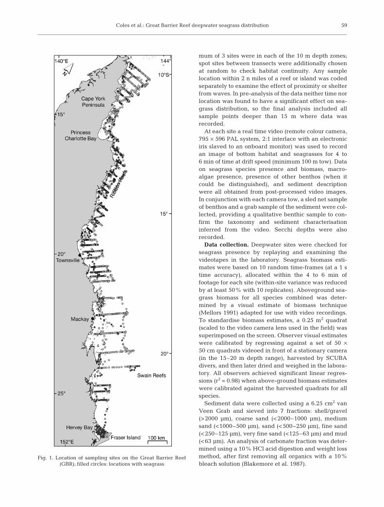
The sampling area included the inter-reef andlagoon waters (from the 15 m contour seaward to theouter barrier reefs, or to the inner edge of the RibbonReefs in the northern section). Sampling included theGBR from the tip of Cape York Peninsular (10°S) toHervey Bay (25°S); approximately 1000 nautical miles(n miles) of coastline extending to just below the GBRin the south. (Fig. 1).

Sampling was stratified in 10 m depth zones from the15 m contour down (15–25, 25–35, 35–45, 45–55, and55–65 m etc.). Recorded depths were adjusted to meansea level by reference to the nearest located tidal planedatum (Queensland Transport 1994–1999) and time ofmeasurement. Two or three cross-shelf transects wererandomly located within every 1° of latitude, with theconstraint that any location less that a minimum of 10 nmiles from a transect location already chosen wasrejected. Sites were randomly selected within a dis-tance increment along each transect, such that a mini-

58

Coles et al.: Great Barrier Reef deepwater seagrass distribution

mum of 3 sites were in each of the 10 m depth zones;spot sites between transects were additionally chosenat random to check habitat continuity. Any samplelocation within 2 n miles of a reef or island was codedseparately to examine the effect of proximity or shelterfrom waves. In pre-analysis of the data neither time norlocation was found to have a significant effect on sea-grass distribution, so the final analysis included allsample points deeper than 15 m where data wasrecorded.

At each site a real time video (remote colour camera,795 × 596 PAL system, 2:1 interlace with an electroniciris slaved to an onboard monitor) was used to recordan image of bottom habitat and seagrasses for 4 to6 min of time at drift speed (minimum 100 m tow). Dataon seagrass species presence and biomass, macro-algae presence, presence of other benthos (when itcould be distinguished), and sediment descriptionwere all obtained from post-processed video images.In conjunction with each camera tow, a sled net sampleof benthos and a grab sample of the sediment were col-lected, providing a qualitative benthic sample to con-firm the taxonomy and sediment characterisationinferred from the video. Secchi depths were alsorecorded.

Data collection. Deepwater sites were checked forseagrass presence by replaying and examining thevideotapes in the laboratory. Seagrass biomass esti-mates were based on 10 random time-frames (at a 1 stime accuracy), allocated within the 4 to 6 min offootage for each site (within-site variance was reducedby at least 50% with 10 replicates). Aboveground sea-grass biomass for all species combined was deter-mined by a visual estimate of biomass technique(Mellors 1991) adapted for use with video recordings.To standardise biomass estimates, a 0.25 m2 quadrat(scaled to the video camera lens used in the field) wassuperimposed on the screen. Observer visual estimateswere calibrated by regressing against a set of 50 ×50 cm quadrats videoed in front of a stationary camera(in the 15–20 m depth range), harvested by SCUBAdivers, and then later dried and weighed in the labora-tory. All observers achieved significant linear regres-sions (r2 = 0.98) when above-ground biomass estimateswere calibrated against the harvested quadrats for allspecies.

Sediment data were collected using a 6.25 cm2 vanVeen Grab and sieved into 7 fractions: shell/gravel(>2000 µm), coarse sand (<2000–1000 µm), mediumsand (<1000–500 µm), sand (<500–250 µm), fine sand(<250–125 µm), very fine sand (<125–63 µm) and mud(<63 µm). An analysis of carbonate fraction was deter-mined using a 10% HCl acid digestion and weight lossmethod, after first removing all organics with a 10%bleach solution (Blakemore et al. 1987).

59

Fig. 1. Location of sampling sites on the Great Barrier Reef (GBR); filled circles: locations with seagrass


Data on the location of trawl effort was extractedfrom Primary Industries and Fisheries, Queensland(PI&F) compulsory commercial daily logbook data base(CFISH) of trawl fishing log records based on a within6 min grid (latitude and longitude) location. GreatBarrier Reef Marine Park (GBRMP) zoning informationwas from an ArcMap (ESRI) data layer of GBRMP zon-ing boundaries.

Statistical analysis. Spatial distributions of the pres-ence/absence of seagrass species were mapped usinggeneralized additive models (GAMs) with binomialerror and smoothed terms (Wood 2004) in relative dis-tance across and along the GBR. Latitude and longi-tude would normally be used for the spatial componentof such models; however, the physical and ecologicalgradients typically run across and (to a lesser degree)along the shelf. Relative distance across the GBR wasdefined as the distance of a site to the coast, divided bythe sum of distances to the coast and to the outer edgeof the GBR. Relative distance along the GBR was simi-larly defined as: the distance to the northern enddivided by the sum of distances to the northern andsouthern ends of the GBR. The coordinates of theacross/along system are locally orthogonal, and run atright angles and parallel to the coast, taking advantageof the fact that many processes are affected by the nat-ural geometry of the GBR.

Predictive models of presence/absence of speciesbased on spatial and environmental variables weremodelled using (aggregated) boosted trees (BTs) withbinomial error (Friedman 2001, De’ath 2007, Fabricius& De’ath 2008). BTs were used for prediction (ratherthan GAMs) since substantial amounts of environmen-tal data were not available; such data is bet-ter handled by BTs, which are also widelyrecognised as being very effective predic-tors (De’ath 2007). All analyses used the Rstatistical package (R Development CoreTeam, 2006).

RESULTS

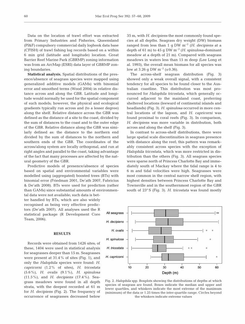
Records were obtained from 1426 sites; ofthese, 1404 were used in statistical analysisfor seagrasses deeper than 15 m. Seagrasseswere present at 31.4% of sites (Fig. 1), andonly the Halophila species were found: H.capricorni (1.2% of sites), H. tricostata(5.6%), H. ovalis (9.1%), H. spinulosa(11.5%), and H. decipiens (17.4%). Sea-grass meadows were found in all depthstrata, with the deepest recorded at 61 mfor H. decipiens (Fig. 2). The frequency ofoccurrence of seagrasses decreased below

35 m, with H. decipiens the most commonly found spe-cies at all depths. Seagrass dry weight (DW) biomassranged from less than 1 g DW m–2 (H. decipiens at adepth of 61 m) to 45 g DW m–2 (H. spinulosa-dominantmeadow at a depth of 21 m). Compared with seagrassmeadows in waters less than 15 m deep (Lee Long etal. 1993), the overall mean biomass for all species waslow at 3.26 g DW m–2 (±0.36).

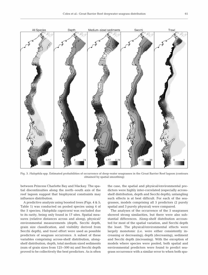
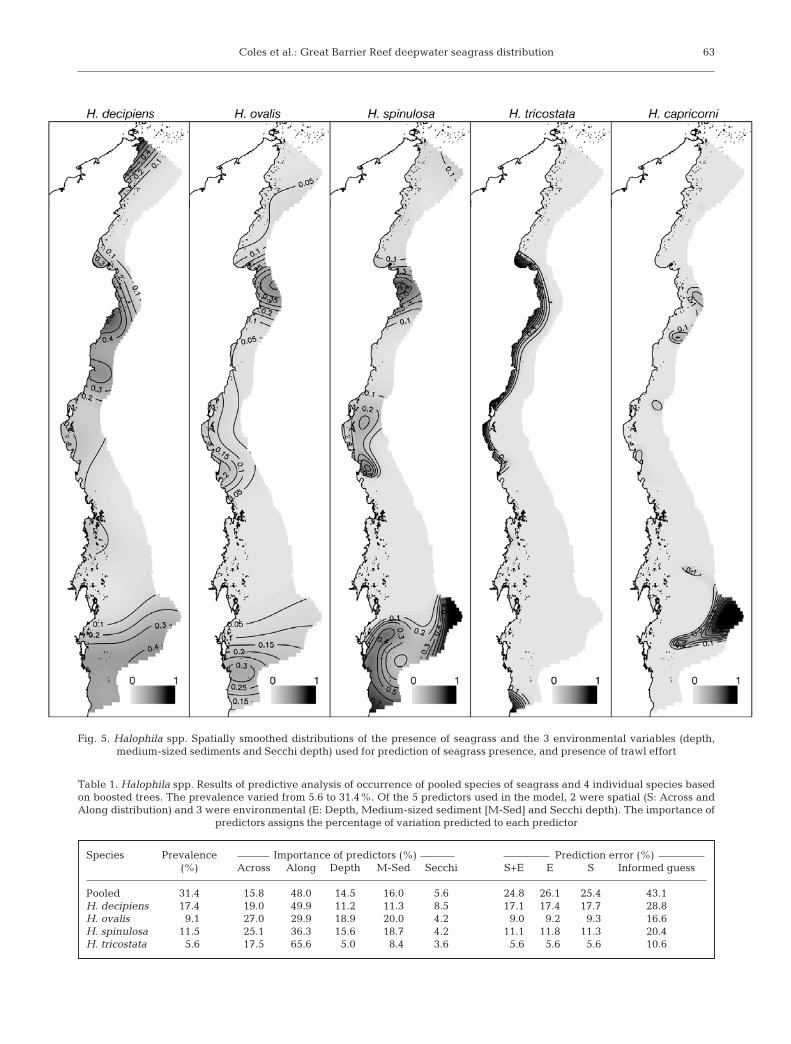
The across-shelf seagrass distribution (Fig. 3)showed only a weak overall signal, with a consistenttendency for all species to be found closer to the Aus-tralian coastline. This distribution was most pro-nounced for Halophila tricostata, which generally oc-curred adjacent to the mainland coast, preferringsheltered locations (leeward of continental islands andheadlands) (Fig. 3). H. spinulosa occurred in more cen-tral locations of the lagoon, and H. capricorni wasfound proximal to coral reefs (Fig. 3). In comparison,H. decipiens was more variable in distribution, bothacross and along the shelf (Fig. 3).

In contrast to across-shelf distributions, there werelarge spatial scale discontinuities in seagrass presencewith distance along the reef; this pattern was remark-ably consistent across species with the exception ofHalophila tricostata, which was more restricted in dis-tribution than the others (Fig. 3). All seagrass specieswere sparse north of Princess Charlotte Bay and imme-diately south of Mackay where the tidal range is 4 to6 m and tidal velocities were high. Seagrasses weremost common in the central narrow shelf region, withhighest densities between Princess Charlotte Bay andTownsville and in the southernmost region of the GBRsouth of 23° S (Fig. 3). H. tricostata was found mostly

60

Fig. 2. Halophila spp. Boxplots showing the distributions of depths at whichspecies of seagrass are found. Boxes indicate the median and upper andlower quartiles, and whiskers indicate the most extreme of the maximum(minimum) of the data or 1.25 times the inter-quartile range. Circles beyond

the whiskers indicate extreme values


between Princess Charlotte Bay and Mackay. The spa-tial discontinuities along the north–south axis of thereef lagoon suggest that biophysical constraints mayinfluence distribution.

A predictive analysis using boosted trees (Figs. 4 & 5;Table 1) was conducted on pooled species using 4 ofthe 5 species; Halophila capricorni was excluded dueto its rarity, being only found in 17 sites. Spatial mea-sures (relative distances across and along), physical/environmental measurements (depth, Secchi depth,grain size classification, and visibility derived fromSecchi depth), and trawl effort were used as possiblepredictors of seagrass occurrence. A subset of thesevariables comprising across-shelf distribution, along-shelf distribution, depth, total medium sized sediments(sum of grain sizes from 125–500 m) and Secchi depthproved to be collectively the best predictors. As is often

the case, the spatial and physical/environmental pre-dictors were highly inter-correlated (especially across-shelf distribution, depth and Secchi depth); untanglingsuch effects is at best difficult. For each of the sea-grasses, models comprising all 5 predictors (2 purelyspatial and 3 purely physical) were compared.

The analyses of the occurrence of the 5 seagrassesshowed strong similarities, but there were also sub-stantial differences. Along-shelf distribution accoun-ted for most of the spatial variation, and Secchi depththe least. The physical/environmental effects werelargely monotonic (i.e. were either consistently in-creasing or decreasing); depth (decreasing), sedimentand Secchi depth (increasing). With the exception ofmodels where species were pooled, both spatial andenvironmental predictors were found to predict sea-grass occurrence with a similar error to when both spa-

61

Fig. 3. Halophila spp. Estimated probabilities of occurrence of deep-water seagrasses in the Great Barrier Reef lagoon (contoursobtained by spatial smoothing)


tial and environmental predictors were combined. Allmodels predicted occurrence with an error rate close tohalf of that based on informed guessing (i.e. guessingrandomly but concurring to the observed prevalence).Models comprising all 5 predictors were only margin-ally better than purely spatial or purely physical/envi-ronmental models (Table 1).

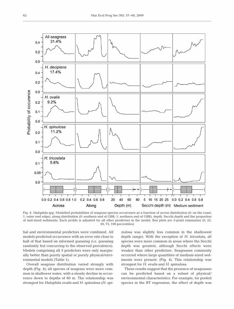
Overall seagrass distribution varied strongly withdepth (Fig. 4); all species of seagrass were more com-mon in shallower water, with a steady decline in occur-rence down to depths of 60 m. The relationship wasstrongest for Halophila ovalis and H. spinulosa (H. spi-

nulosa was slightly less common in the shallowestdepth range). With the exception of H. tricostata, allspecies were more common in areas where the Secchidepth was greatest, although Secchi effects wereweaker than other predictors. Seagrasses commonlyoccurred where large quantities of medium-sized sed-iments were present. (Fig. 4). This relationship wasstrongest for H. ovalis and H. spinulosa.

These results suggest that the presence of seagrassescan be predicted based on a subset of physical/environmental characteristics. For example, for pooledspecies in the BT regression, the effect of depth was

62

Fig. 4. Halophila spp. Modelled probabilities of seagrass species occurrence as a function of across distribution (0: on the coast;1: outer reef edge), along distribution (0: southern end of GBR; 1: northern end of GBR), depth, Secchi depth and the proportionof mid-sized sediments. Each profile is adjusted for all other predictors in the model. Box plots are 5-point summaries (0, 25,

50, 75, 100 percentiles)

Coles et al.: Great Barrier Reef deepwater seagrass distribution 63

Table 1. Halophila spp. Results of predictive analysis of occurrence of pooled species of seagrass and 4 individual species basedon boosted trees. The prevalence varied from 5.6 to 31.4%. Of the 5 predictors used in the model, 2 were spatial (S: Across andAlong distribution) and 3 were environmental (E: Depth, Medium-sized sediment [M-Sed] and Secchi depth). The importance of

predictors assigns the percentage of variation predicted to each predictor

Species Prevalence Importance of predictors (%) Prediction error (%)(%) Across Along Depth M-Sed Secchi S+E E S Informed guess

Pooled 31.4 15.8 48.0 14.5 16.0 5.6 24.8 26.1 25.4 43.1H. decipiens 17.4 19.0 49.9 11.2 11.3 8.5 17.1 17.4 17.7 28.8H. ovalis 9.1 27.0 29.9 18.9 20.0 4.2 9.0 9.2 9.3 16.6H. spinulosa 11.5 25.1 36.3 15.6 18.7 4.2 11.1 11.8 11.3 20.4H. tricostata 5.6 17.5 65.6 5.0 8.4 3.6 5.6 5.6 5.6 10.6

Fig. 5. Halophila spp. Spatially smoothed distributions of the presence of seagrass and the 3 environmental variables (depth, medium-sized sediments and Secchi depth) used for prediction of seagrass presence, and presence of trawl effort


strongest, increasing the odds of presence of seagrassincreasing by a factor of 9 (equivalent to a shift fromp = 0.1 to p = 0.5) in shallow depths (15 m) comparedwith the deep (60 m). For medium sediments, the oddsof seagrass being present increased by a factor of 6(equivalent to a shift from p = 0.17 to p = 0.5) for 80%compared with 5% medium-sized sediments, and forSecchi depth there was a weaker relationship — theodds of presence of an increase in the probability ofpresence of seagrass for a shift in Secchi distance from5 to 25 m depth was 3.5 (equivalent to a shift from p =0.15 to p = 0.35).

Using the model that only included spatial and depthvariables and making the assumption that the reeflagoon is divided into units of 500 m2 (an individualvideo tow area), the mean probability of seagrassbeing present was 0.38, and 23% of those 500 m2 unitswould have a probability of >0.5 for the presenceof seagrass. This would be equivalent to ~40 000 km2 oflagoon and inter-reef area within the GBR provincehaving at least a chance of some seagrass being pre-sent.

When overlaid on the distribution of trawl fishingeffort (which is recorded in grids of 6 min of latitudeand longitude) there is considerable overlap; 42% ofthe grids with catch recorded in 1999 have a >50%chance of seagrass occurrence, and only 29% ofgrids have a <50% chance of seagrass occurrence aretrawled (Fig. 5).

Within the GBR, ~33% of the seagrass area pre-dicted to be present in this study is now included inhighly protected no-take zones, and between 50 and60% is in an area not allowed for trawl fishing (or is inan area where trawling does not take place due tosome physical or operational constraint). For areas ofthe GBR with a greater than 50% chance of seagrassoccurrence, modelled trawl data (from electronic mon-itoring of the Queensland East Coast Trawl Fishery;Coles et al. 2008) shows that only 36.3% is nowtrawled, and only 14% is trawled more than once inany one year under present management arrange-ments.

DISCUSSION

Approach to mapping

Making spatial sense of seagrass distributions overan area as large, and in water as deep, as in the GBRprovince is an enormous challenge. Ideally, themeadow types should be aerially photographed andmapped, with species composition characterised andedge-mapped by GPS (as would be the approach forintertidal seagrass). As this is not possible, we have

only the option to infer distributions from point sourcedata, and by investigating mathematical correlations tomake some sense of them; in effect, a modelingmethod is used as a surrogate for remote sensing.

The sheer size of the task is compounded by thepotential for temporal variability both within andbetween years, and by inferences necessarily drawnfrom a relatively sparse data density and in theabsence of any defined seagrass meadow edges. Timeand logistics made it impossible to complete the sur-veys within a season for any one year, or to repeatwidely dispersed samples across years. There was no apriori reason (unusual weather, etc.) to expect annualGBR-wide differences in deep-water seagrasses overthe time of the study; the much more intensively sam-pled coastal seagrasses in the GBR remain relativelyconstant through time (Coles et al. 2007). Previousstudies in the reef lagoon have shown little changeother than slight increases over a 12 yr period; almostcertainly the result of improved sampling technique(Coles et al. 2002, 2007). A comparison between thisstudy and a more recent biodiversity study of the GBRlagoon (Pitcher et al. 2007) shows that the strong spa-tial patterns accounted for 79% of the spatial and tem-poral variation over a 10 yr period, with only 21% dueto variation over time (De’ath et al. 2007).

Seagrass species

Finding only one genus of seagrass (Halophila) was asurprising result, although all of the seagrass speciesthat were found are common in the GBR. There are15 seagrass species in Queensland waters, represent-ing 9 genera; some genera (such as Enhalus and Rup-pia) are restricted to shallow inshore waters and wouldnot be expected in deep-water collections. Thalasso-dendron is usually found associated with reefs. Other(mostly inshore) genera were expected in the distribu-tions, albeit in small numbers. Halophila spp. haveclearly adapted to survive in the low light conditions ofdeeper waters in the region, and completely dominatethis environment.

Halophila tricostata is a species considered to beendemic to northern Australia (Greenway 1979, Kuo etal. 1993). It has a clumped distribution in this surveyand is mostly found close to the coast on medium-sizedterrigenous sediments in the central wet tropic area(between Princess Charlotte Bay and Townsville), withsome meadows as far south as Mackay. It was amongthe least known of the Halophila species (Kuo et al.1993), but is now shown to be common in the GBRlagoon, highlighting the extent and importance of thereef lagoon seagrass community as an ecological com-ponent of the biodiversity of coastal waters.

64


Halophila capricorni is found only in the southernIndo-Pacific (Larkum 1995); it is uncommon, and itsabsence from shallow water collections means it israrely seen. All other species are broadly distributedthroughout the Indo-Pacific region (Fortes 1989, Short& Coles 2001).

Compared with intertidal above-ground biomassmeasurements from seagrass meadows in Queensland,3 g DW m–2 is low. Halophila spinulosa and H. tri-costata at times formed large and dense meadows. Themajority of samples were of isolated plants or of speci-mens that were very small-leaved species in the Halo-phila genus. Low light levels in deep water influencenot only the species suite, but also biomass. H. spinu-losa had the largest biomass found, at a depth of 21 m.Both H. spinulosa and H. tricostata are di-meristematicnon-leaf-replacing species with an erect stem. Theyare able to produce additional new leaves on a shootduring the life of the plant (Short & Duarte 2001),allowing them to increase the surface area of a leafcluster; this maximises photosynthesis in response tolow light conditions, and has the effect of contributingto a greater above-ground biomass.

Spatial representation

Prior to this study there was little to suggest largemeadows of seagrass existed within the GBR lagoon inwater deeper than 15 m; coastal meadows in Queens-land had only been surveyed down to 15–20 m, andthese were intermittent and of low biomass at the outeredge, even at these depths. There are few otherreports of seagrass meadows as extensive as thosefound at these depths in the GBR from around theworld. Den Hartog (1970) reported Halophila decipi-ens to 85 m with records deeper than 50 m in the GBR,Seychelles and Cargados Carajos (Mauritius), butmade no attempt to assess the extent of the meadows.Fourqurean et al. (2001), Hammerstrom et al. (2006)and Fonseca et al. (2008) have described aspects of a20 000 km2 seagrass meadow on the west Florida shelf,USA. This meadow extends down to the 35 m isobath,although the outer edge is poorly delineated and couldpresumably extend deeper. The Florida meadows haveonly one species (H. decipiens) in common with ourstudy, and this has a much greater coverage and den-sity, so making comparisons difficult. However the factthat large meadows of seagrass are found in deepwater in such (e.g. see Kenworthy et al. 1989) widelyseparated parts of the world, Florida and northeastAustralia, suggests that other deep water meadows arelikely to exist, particularly in the tropics.

The natural geometry of the GBR and its lagoon (along strip, shallow at the reef edge and coast and deep

in the middle) forces the geometry of habitat typessuch as seagrass meadow to run in long NW to SEstrips. Because of this geometry, it was assumed in thesampling design that there would be distinct bands ofmeadow across the narrow E–W axis, with specieszonation reflecting the mirrored depth zones in theouter and inner reef lagoon; these were assumed to bemore or less consistent throughout the N–S axis. How-ever, the E–W banding was more a concentration ofseagrasses within a 15–25 m depth band of the west-ern edge of the lagoon; this area is associated with thepresence of terrigenous sediments and mid-range par-ticle sizes. The shallow eastern lagoon, with coarsecoralline and Halimeda sands and probably low nutri-ent availability (Udy et al. 1999), supports patchy sea-grass meadows of very low biomass.

There are however very strong spatial discontinu-ities in seagrass meadows along the N–S axis, andthese spatial effects alone explain much of the overallvariation in seagrass distribution. Seagrasses wereuncommon north of Princess Charlotte Bay, a remotearea of low human population and little disturbance.The East Australian Current diverges at Princess Char-lotte Bay with deep oceanic water flowing shorewardsand splitting north and south (Church 1987), and it ispossible there is recruitment limitation. Much of thecoast north of the Princess Charlotte Bay coast is alsosilica sand and low in stream run-off, possibly limitingthe availability of nutrients for seagrass growth.

Seagrasses formed extensive meadows in a bandfrom Princess Charlotte Bay to just south of Townsville.All species were found in this region which abuts thecoastal wet tropics with a moderate tidal range, highannual rainfall and numerous coastal rivers, as well asestuaries (many of which have extensive mangroveforests and large intertidal and shallow subtidal sea-grass meadows). There are suitable areas of seafloor ata depth where seagrass can grow, a large supply ofpotential reproductive material (seeds and vegetativefragments), and ample nutrient input to sustain sea-grass growth (Schaffelke et al. 2005). This is a highlyproductive coastal region mirrored in the adjacentshallow reef lagoon by the extensive seagrass mead-ows. South of Townsville the extent of seagrass pres-ence declines until reaching an area of large tidalranges (up to 6 m) just to the south of Mackay, whereno major deepwater seagrass meadows exist. This is aregion of high current stress, low Secchi readings andcoarse mobile sediments; habitat unsuitable for sea-grass growth.

The predictive spatial analysis demonstrates surpris-ingly good accuracy (74%) based on depth, sedimentand visibility measured by Secchi depth (Table 1). The2 areas where analysis does not accurately predict sea-grass presence is in the very north and in the offshore

65


region to the south in the Swain Reef area. Bothregions are remote from available reproductive mater-ial, and in regions very low in nutrients or removedfrom the coast. Physically, seagrass could grow in theseregions, but that is likely to be prevented by biologicalconstraints specific to those areas. While a ‘map’ ofseagrass derived from physical surrogates may providea reasonable guide to the likelihood of seagrass pres-ence, local effects will always be difficult to include ina model that describes such a large area; a certainlevel of uncontrolled error would always have to beallowed for in such a predictive model. Nevertheless,the predictive ‘map’ generated by the model is a goodfirst approximation of seagrass distribution. This sug-gests that simple spatial and environmental surrogatescan be used to explore the possibility of seagrass intropical deep-water environments on the coastal shelf,and to ‘map’ potential areas of seagrass meadows atother locations with similar species.

The ecological role of inter-reef seagrasses and asso-ciated algal meadows at these depths is not wellunderstood (Carruthers et al. 2002); it is likely theyprovide ecosystem services similar to those providedby the coastal and intertidal seagrasses that have beenextensively studied worldwide. It is possible productiv-ity is low compared to seagrass meadows in shallowwaters (Primary Industries & Fisheries unpubl. data),but this effect would be offset by the very large areasfound.

Management implications

The seagrass and benthic community database fromthis sampling program was one of the major databasesthat supported development of a multi-use zoning planin the GBR, the Representative Areas Plan (Kenworthyet al. 2006). This was designed to maintain reef biodi-versity, and to determine the location of activities inthe Great Barrier Reef Marine Park.

When all spatial closures are included, bottomtrawling is now restricted to just 34% of the park(Coles et al. 2008). There is also an informal agree-ment by the commercial fishing industry that trawloperators will avoid areas of known seagrass mead-ows, and repeated trawling in grids with seagrass isnot common (with only 14% of grids trawled morethan once in a fishing season). However, trawling iscommon in the 6 minute (latitude, longitude) fishinggrids where seagrass was recorded, and less commonwhere there was no seagrass. This is probably a scaledependent result, as the fishing grids are very largeand seagrass may occur within a grid without beingaffected by trawlers operating on smaller scale fishinggrounds. It may also be simple spatial coincidence,

with both trawling and seagrass tending to occur onbottom areas with shallow to medium depths andopen soft sediments.

Conversely, it is possible that the low intensity bot-tom trawling (that occurs in most of the survey area)transports viable seagrass vegetative fragments tonew sites, or may stimulate growth in situ throughdisturbance of the seed bank. Halophila ovalis andH. decipiens produce their seeds at or below the sur-face of marine sediments, where they are unavail-able for immediate dispersal (Inglis 2000). Seeds ofHalophila are persistent, and under laboratory condi-tions can remain viable for up to 2 yr (Inglis 2000).Laboratory germination trials have shown that seedsof at least 4 species of Halophila germinate whenthey are exposed to light (Inglis 2000), and that lightexposure and day length are important in success-ful flowering and seed production (McMillan 1976).Seagrass seed banks for species such as H. decipienscan be comparable in size to the largest seed banksreported for tropical forests and grasslands, and mayhave an important ecological role in maintainingthese seagrass ecosystems (Hammerstrom et al.2006).

It has been established worldwide that bottom-fishing activities involving the use of mobile gear havea physical impact upon the seabed and the biota thatlive there (Kaiser et al. 2002). However, our study indi-cates that at the scale of the whole of GBR, trawling thebottom for penaeid shrimp and scallop over the last40 yr has not reduced the probability of finding sea-grass to levels less than that found in the non-trawledareas.

Changes in GBR deepwater seagrasses are notdetectable by surface observation, and large areascould be lost before secondary ecological signals werenoticed. Changes in light penetration and the possibleeffects of climate change (such as increased run-offand turbidity) will be integrated by the plants overlong time scales in this region, and changes in distrib-ution patterns, particularly the location of the deepedge, would be a valuable indicator for any long-termclimate change.

Acknowledgements. The authors are very grateful to G. Chis-holm, P. Leeson and C. Cant for support in the vessel-basedsampling program. We thank the many people who assistedus in the field and laboratory, including: P. Daniel, C. Roder,M. Rasheed, K. Vidler, M. Short, A. Grice, B. Deeley,C. Shootingstar, J. Slater, L. Makey, R. Bennett, R. Thomas,S. Hollywood and V. Hall. We also thank T. Done, G. Inglis,H. Marsh, B. Mapstone, C. Crossland, J. Phillips, J. Mellorsand D. Reid for comments on sampling design. This projectwas funded by the CRC Reef Research Centre, the GreatBarrier Reef Marine Park Authority and the QueenslandPrimary Industries & Fisheries.

66


LITERATURE CITED

Blakemore, LC, Serale PL, Daly BR (1987) Methods of chemi-cal analysis of soils. NZ Soil Bur, Sci Rep 80

Carruthers TJB, Dennison WC, Longstaff BJ, Waycott M, AbalEG, McKenzie LJ, Lee Long WJ (2002) Seagrass habitatsof northeast Australia: models of key processes and con-trols. Bull Mar Sci 71:1153–1169

Church JA (1987) East Australian Current adjacent to theGreat Barrier Reef. Aust J Mar Freshw Res 38:671–683

Coles RG, Lee Long WJ, Squire BA, Squire LC, Bibby JM(1987) Distribution of seagrasses and associated juvenilecommercial penaeid prawns in north-eastern Queenslandwaters. Aust J Mar Freshw Res 38:103–119

Coles RG, Lee Long WJ, Watson RA, Derbyshire KJ (1993)Distribution of seagrasses, and their fish and penaeidprawn communities, in Cairns Harbour, a tropical estuary,northern Queensland, Australia. Aust J Mar Freshw Res44:193–210

Coles RG, Lee Long WJ, McKenzie LJ (eds) (2002) Seagrassand marine resources in the Dugong protection areas ofUpstart Bay, Newry Region, Sand Bay, Llewellyn Bay, InceBay and the Clairview Region: April/May 1999 and Octo-ber 1999. Res Publ No 72. Great Barrier Reef Marine ParkAuthority, Townsville

Coles RG, McKenzie LJ, Rasheed MA, Mellors JE and others(2007) Status and trends of seagrass in the Great BarrierReef World Heritage Area: report (PR07–3258) to theMarine and Tropical Sciences Research Facility. Reef andRainforest Research Centre, Cairns

Coles RG, Grech A, Dew K, Zeller B, McKenzie L (2008) Apreliminary report on the adequacy of protection providedto species and benthic habitats in the east coast otter trawlfishery by the current system of closures (PR08–3576).Department of Primary Industries and Fisheries, Brisbane

Costanza R, d’Arge R, de Groot R, Farber S and others (1997)The value of the world’s ecosystem services and naturalcapital. Nature 387:253–260

Day JC, Fernandes L, Lewis A, De’ath G and others (2000)The representative area program for protecting biodiver-sity in the Great Barrier Reef World Heritage Area. Proc9th Int Coral Reef Symp 2:687–696

De’ath G (2007) Boosted trees for ecological modeling andprediction. Ecology 88:243–251

De’ath G, Coles RG, McKenzie L, Pitcher R (2007) Spatial distributions and temporal change in distributions of deepwater seagrasses in the Great Barrier Reef region. Reportto the Marine and Tropical Sciences Research Facility.Reef and Rainforest Research Centre, Cairns

Den Hartog C (1970) The seagrasses of the world. North-Holland, Amsterdam

Fabricius KE, De’ath G (2008) Photosynthetic symbionts andenergy supply determine octocoral biodiversity in coralreefs. Ecology 89:3163–3173

Fonseca MS, Kenworthy JW, Griffith E, Hall MO, FinkbeinerM, Bell SS (2008) Factors influencing landscape pattern ofthe seagrass Halophila decipiens in an oceanic setting.Estuar Coast Shelf Sci 76:163–174

Fortes MD (1989) Seagrasses: a resource unknown in theASEAN region. ICLARM Education Series Vol 5. Interna-tional Centre for Living Aquatic Resources Management,Manila

Fourqurean JW, Willsie A, Rose CD, Rutten LM (2001) Spatialand temporal pattern in seagrass community compositionand productivity in South Florida. Mar Biol 138:341–354

Friedman JH (2001) Greedy function approximation: a gradi-ent boosting machine. Ann Stat 29:1189–1232

Greenway M (1979) Halophila tricostata (Hydrocharitaceae),a new species of seagrass from the Great Barrier Reefregion. Aquat Bot 7:67–70

Hammerstrom KK, Kenworthy JW, Fonseca MS, Whitfield PE(2006) Seed bank, biomass and productivity of Halophiladecipiens, a deep water seagrass on the west Florida con-tinental shelf. Aquat Bot 84:110–120

Inglis GJ (2000) Variation in the recruitment behaviour of sea-grass seeds: implications for population dynamics andresource management. Pac Conserv Biol 5:251–259

Kaiser MJ, Collie JS, Hall SJ, Jennings S, Poiner IR (2002)Modification of marine habitats by trawling activities:prognosis and solutions. Fish Fish 3:114–136

Kenworthy WJ, Currin CA, Fonseca MS, Smith G (1989) Pro-duction, decomposition, and heterotrophic utilization ofthe seagrass Halophila decipiens in a submarine canyon.Mar Ecol Prog Ser 51:277–290

Kenworthy WJ, Wyllie-Echeverria S, Coles RG, Pergent G,Pergent C (2006) Seagrass conservation biology: an inter-disciplinary science for protection of the seagrass biome.In: Larkum (eds) Seagrass biology, ecology and conserva-tion. Springer, Dordrecht, p 595–623

Kuo J, Lee Long W, Coles RG (1993) Fruits and seeds ofHalophila tricostata Greenway (Hydrocharitacea) withspecial notes on its occurrence and biology. Aust J MarFreshw Res 44:43–57

Lanyon JM, Limpus CJ, Marsh H (1989) Dugongs and turtles:grazers in the seagrass system. In: Larkum AWD,McComb AJ, Shepherd SA (eds) Biology of seagrasses:a treatise on the biology of seagrasses with specialreference to the Australian region. Elsevier, Amsterdam,p 610–634

Larkum AWD (1995) Halophila capricorni (Hydrocharita-ceae): a new species of seagrass from the coral sea. AquatBot 51:319–328

Larkum AWD, Orth RJ, Duarte CM (2006) Seagrasses: biol-ogy, ecology and conservation. Springer, Dordrecht

Lee Long WJ, Mellors JE, Coles RG (1993) Seagrassesbetween Cape York and Hervey Bay, Queensland, Aus-tralia. Aust J Mar Freshw Res 44:19–31

McKenzie LJ, Finkbeiner MA, Kirkman H (2001) Methods formapping seagrass distribution. In: Short FT, Coles RG(eds) Global seagrass research methods, Chap 5. Elsevier,Amsterdam, p 101–122

McMillan C (1976) Experimental studies on flowering andreproduction in seagrasses. Aquat Bot 2:87–92

Mellors JE (1991) An evaluation of a rapid visual techniquefor estimating seagrass biomass. Aquat Bot 42:67–73

Orth RJ, Carruthers TJB, Dennison WC, Duarte CM (2006)Global crises for seagrass ecosystems. Bioscience 56:987–997

Pitcher CR, Doherty P, Arnold P, Hooper J and others (2007)Seabed biodiversity on the continental shelf of the GreatBarrier Reef World Heritage Area. AIMS/CSIRO/QM/DPICRC Reef Research Task final report, CSIRO Marine andAtmospheric Research, Cleveland, QLD

Queensland Transport (1994–1999) The official tide tablesand boating guide. Queensland Transport, Brisbane

R Development Core Team (2006) R: a language and environ-ment for statistical computing. R Foundation for StatisticalComputing, Vienna

Schaffelke B, Mellors J, Duke N (2005) Water quality in theGreat Barrier Reef region: responses of mangrove, sea-grass and macroalgal communities. Mar Pollut Bull 51:279–296

Short FT, Coles RG (eds) (2001) Global seagrass researchmethods. Elsevier, Amsterdam

67


Short FT, Duarte CM (2001) Methods of the measurement ofseagrass growth and production. In Short FT, Coles RG(eds) Global seagrass research methods. Elsevier, Amster-dam, p 154–182

Udy JW, Dennison WC, Lee Long WJ, McKenzie LJ (1999)Responses of seagrass to nutrients in the Great BarrierReef, Australia. Mar Ecol Prog Ser 185:257–271

Wachenfeld DR, Oliver JK, Morrissey JI (eds) (1998) State ofthe Great Barrier Reef World Heritage Area 1998. GreatBarrier Reef Marine Park Authority, Townsville

Watson RA, Coles RG, Lee Long WJ (1993) Simulation esti-

mates of annual yield and landed value for commercialpenaeid prawns from a tropical seagrass habitat, north-ern Queensland, Australia. Aust J Mar Freshw Res 44:211–220

Williams LE (2002) Queensland’s fisheries resources. Currentcondition and trends 1988–2000. Information SeriesQI02012, Queensland Department of Primary Industries,Brisbane

Wood SN (2004) Stable and efficient multiple smoothing para-meter estimation for generalized additive models. J AmStat Assoc 99:673–686

68

Editorial responsibility: Kenneth Heck Jr., Dauphin Island, Alabama, USA

Submitted: December 22, 2006; Accepted: July 6, 2009Proofs received from author(s): October 7, 2009

Spatial distribution of deepwater seagrass in the inter ... · The Great Barrier Reef World...

Documents

Transcript of Spatial distribution of deepwater seagrass in the inter ... · The Great Barrier Reef World...