Spatial Clustering Using Hierarchical SOM -...

Chapter 12

Spatial Clustering Using Hierarchical SOM

Roberto Henriques, Victor Lobo andFernando Bação

Additional information is available at the end of the chapter

http://dx.doi.org/10.5772/51159

1. Introduction

The amount of available geospatial data increases every day, placing additional pressure onexisting analysis tools. Most of these tools were developed for a data poor environment andthus rarely address concerns of efficiency, high-dimensionality and automatic exploration[1]. Recent technological innovations have dramatically increased the availability of data onlocation and spatial characterization, fostering the proliferation of huge geospatial databas‐es. To make the most of this wealth of data we need powerful knowledge discovery tools,but we also need to consider the particular nature of geospatial data. This context has raisednew research challenges and difficulties on the analysis of multidimensional geo-referenceddata. The availability of methods able to perform “intelligent” data reduction on vastamounts of high dimensional data is a central issue in Geographic Information Science(GISc) current research agenda.

The field of knowledge discovery constitutes one of the most relevant stakes in GISc re‐search to develop tools able to deal with “intelligent” data reduction [2, 3] and tame com‐plexity. More than prediction tools, we need to develop exploratory tools which enable animproved understanding of the available data [4].

The term cluster analysis encompasses a wide group of algorithms (for a comprehensive re‐view see [5]). The main goal of such algorithms is to organize data into meaningful struc‐tures. This is achieved through the arrangement of data observations into groups based onsimilarity. These methods have been extensively applied in different research areas includ‐ing data mining [6, 7], pattern recognition [8, 9], and statistical data analysis [10]. GISc hasalso relied heavily on clustering algorithms [11, 12]. Research on geodemographics [13-16],identification of deprived areas [17], and social services provision [18] are examples of therelevance that clustering algorithms have within today’s GISc research.

© 2012 Henriques et al.; licensee InTech. This is an open access article distributed under the terms of theCreative Commons Attribution License (http://creativecommons.org/licenses/by/3.0), which permitsunrestricted use, distribution, and reproduction in any medium, provided the original work is properly cited.

One of the most challenging aspects of clustering is the high dimensionality of most prob‐lems. While in general describing phenomena requires the use of many variables, the in‐crease in dimensionality will have a significant impact on the performance of clusteringalgorithms and the quality of the results. First, it will increase the search space affecting theclustering algorithm’s efficiency, due to the effect usually known as the “curse of dimen‐sionality” [19]. Second, it will yield a more complex analysis of the output, as the clusters aremore difficult to characterize due to the contribution of multiple variables to the final struc‐ture. Thus, in a typical clustering problem, the user is asked to select a low number of varia‐bles that optimize the phenomena’s description.

However, to produce an accurate representation of the phenomenon, it is sometimes neces‐sary to measure it from several perspectives. A typical example is the use of census variablesto study the socio-economic environment in an urban context. Usually, the census covers awide range of themes describing the characteristics of the population such as the demogra‐phy, households, families, housing, economic status, among others[20]. In these cases, somevariables are strongly correlated, independently of the subject they are covering. In fact,with the increase in dimensionality, there is a higher probability of correlation between vari‐ables. In addition, due to the spatial context of census data, variables have strong spatial au‐tocorrelation [21]. Spatial autocorrelation measures the degree of dependency amongobservations in a geographic space. This spatial autocorrelation corroborates Tobler’s [22]first law (TFL) which expresses the tendency of nearby objects to be similar.

To GIScientists, clusters are usually more representative and easier to understand if theypresent spatial contiguity. However, several reasons can cause the clusters to present spatialdiscontinuity. Among these, the scale or zoning scheme of the geographical units, known asthe modifiable areal unit problem (MAUP) [23] can affect the expected spatial patterns. Inaddition, the combination of different variables, that presents distinct levels of spatial auto‐correlation, affects the clusters’ spatial patterns.

Traditional clustering methods, in which self-organizing maps [24] are included, are verysensitive to divergent variables. Divergent variables are those that present significant differ‐ences to the general tendency. These variables have a great impact in the clustering processand are crucial in the final partition. For instance, when clustering using a set of variableswhere all, except one, present spatial autocorrelation, the divergent variable will have ahigher impact than the others. In most cases, the clusters created will not follow the spatialarrangement suggested by the majority of the variables, but will get distorted by the varia‐bles presenting odd spatial distributions.

To avoid this problem a hierarchical structure may be used to explore and cluster geospatialdata. Variables are grouped in themes, and each theme will be independently clustered.These partial clusters are then used to create a global partition.

One well-known clustering method is the Self-Organizing Map (SOM) proposed by Koho‐nen [24]. One of the interesting properties of SOM is the capability of detecting small differ‐ences between objects. SOM have proved to be a useful and efficient tool in finding

Applications of Self-Organizing Maps232

multivariate data outliers [25-27]. SOM has also been widely used in the GIScience field inthe exploration and clustering of geospatial data [28-33, 34, 35].

In this chapter, we propose the use of Hierarchical SOMs to perform geospatial clustering.Several characteristics of geospatial data make it a good candidate to benefit from theHSOM specific features. The classic layer organization used in GIScience fits perfectly thelayered structure of HSOM. HSOM provides an appropriate framework to perform the clus‐tering task based on individual themes, which can then be compared with the clusters creat‐ed from the combination of several themes. HSOM is less sensitive to divergent variablesbecause these will only have a direct impact on their theme.

There are many types of hierarchical SOM, so we propose a taxonomy to classify existingmethods according to their objectives and structure.

2. Background

2.1. Self-Organizing Maps

Teuvo Kohonen proposed the Self-organizing maps (SOM) in the beginning of the 1980s[36]. The SOM is usually used for mapping high-dimensional data into one, two, or three-dimensional feature maps. The basic idea of an SOM is to map the data patterns onto an n-dimensional grid of units or neurons. That grid forms what is known as the output space, asopposed to the input space that is the original space of the data patterns. This mapping triesto preserve topological relations, i.e. patterns that are close in the input space will be map‐ped to units that are close in the output space, and vice-versa. The output space is usuallytwo-dimensional, and most of the implementations of SOM use a rectangular grid of units.To provide even distances between the units in the output space, hexagonal grids are some‐times used [24]. Each unit, being an input layer unit, has as many weights as the input pat‐terns, and can thus be regarded as a vector in the same space of the patterns.

When training an SOM with a given input pattern, the distance between that pattern andevery unit in the network is calculated. Then the algorithm selects the unit that is closest asthe winning unit (also known as best matching unit- BMU), and that pattern is mapped onto that unit. If the SOM has been trained successfully, then patterns that are close in the in‐put space will be mapped to units that are close (or the same) in the output space. Thus,SOM is ‘topology preserving’ in the sense that (as far as possible) neighbourhoods are pre‐served through the mapping process.

The basic SOM learning algorithm may be described as follows:

Spatial Clustering Using Hierarchical SOMhttp://dx.doi.org/10.5772/51159

233

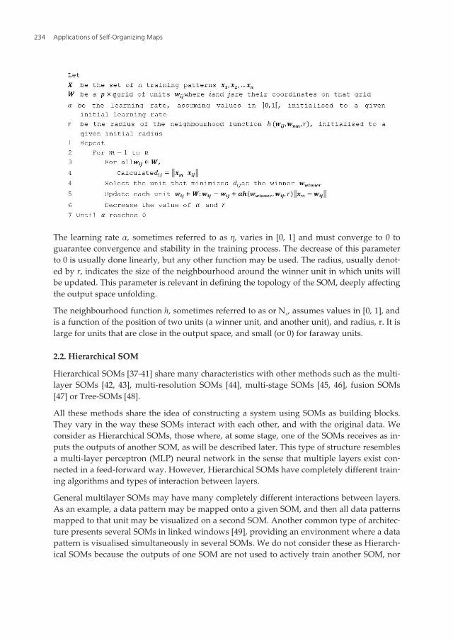
The learning rate α, sometimes referred to as η, varies in [0, 1] and must converge to 0 toguarantee convergence and stability in the training process. The decrease of this parameterto 0 is usually done linearly, but any other function may be used. The radius, usually denot‐ed by r, indicates the size of the neighbourhood around the winner unit in which units willbe updated. This parameter is relevant in defining the topology of the SOM, deeply affectingthe output space unfolding.

The neighbourhood function h, sometimes referred to as or Nc, assumes values in [0, 1], andis a function of the position of two units (a winner unit, and another unit), and radius, r. It islarge for units that are close in the output space, and small (or 0) for faraway units.

2.2. Hierarchical SOM

Hierarchical SOMs [37-41] share many characteristics with other methods such as the multi-layer SOMs [42, 43], multi-resolution SOMs [44], multi-stage SOMs [45, 46], fusion SOMs[47] or Tree-SOMs [48].

All these methods share the idea of constructing a system using SOMs as building blocks.They vary in the way these SOMs interact with each other, and with the original data. Weconsider as Hierarchical SOMs, those where, at some stage, one of the SOMs receives as in‐puts the outputs of another SOM, as will be described later. This type of structure resemblesa multi-layer perceptron (MLP) neural network in the sense that multiple layers exist con‐nected in a feed-forward way. However, Hierarchical SOMs have completely different train‐ing algorithms and types of interaction between layers.

General multilayer SOMs may have many completely different interactions between layers.As an example, a data pattern may be mapped onto a given SOM, and then all data patternsmapped to that unit may be visualized on a second SOM. Another common type of architec‐ture presents several SOMs in linked windows [49], providing an environment where a datapattern is visualised simultaneously in several SOMs. We do not consider these as Hierarch‐ical SOMs because the outputs of one SOM are not used to actively train another SOM, nor


does the second SOM, in any way, use information from the first map to map the originaldata patterns.

We consider that, to be recognized as a Hierarchical SOM, the interaction between differentSOMs must be of the train/map type. This type of interaction is one where the outputs ofone SOM are used to train the other SOM, and this second one maps (represents) the origi‐nal data patterns using the outputs of the first one. If these two characteristics are notpresent, we consider we do not have a true Hierarchical SOM, because it is the train/maprelationship that establishes a strict subordination between SOMs that in turn is necessaryfor a hierarchy to exist.

The train/map type of interaction encompasses different specific ways of passing informa‐tion from one SOM to another. As an examples, when a data pattern is presented to the firstlevel SOM, it may pass the information onto the second level by passing the index of thebest matching unit (BMU), the quantization error, the coordinates of the BMU, all activationvalues for all units of the first level, or any other type of data. The important issue is thatwhatever data is passed on, it is used to train the second level SOM. A particular case ofoutput of one SOM layer may be the original data pattern itself, or an empty data pattern.This is the case of a first level gating SOM that filters which data patterns are sent to eachupper level SOM: it may or may not pass the pattern, depending on some characteristic.

Still, many different configurations are possible for Hierarchical SOMs. They may vary inthe number of layers used, in the different ways connections are made and even in the infor‐mation sent through each connection.

2.3. Why use Hierarchical SOMs (HSOM)?

There are mainly two reasons for using a Hierarchical SOM (HSOM) instead of a standardSOM:

• A HSOM can require less computational effort than a standard SOM to achieve certaingoals;

• A HSOM can be better suited to model a problem that has, by its own nature, some sort ofhierarchical structure.

The reduction of computational effort can be achieved in two ways: by reducing the dimen‐sionality of the inputs to each SOM, and by reducing the number of units in each SOM. In‐stead of having a SOM that uses all components of the input patterns, we may have severalSOMs, each using a subset of those components, and in this way we minimize the effect ofthe “curse of dimensionality” [19]. The distance functions used for training the differentSOMs will be simpler, and thus faster to compute. This simplicity will more than compen‐sate for the increase in the number of different functions that have to be computed. Speedgains can also be achieved by using fewer units in each SOM. The finer distinction betweendifferent clusters (units) can be achieved in upper level SOMs that will only have to dealwith some of the input patterns. This “divide and conquer” strategy will avoid computing


235

distances and neighbourhoods to units that are very different from the input patterns beingprocessed in each instant.

The second reason for using HSOMs is that, in general, they are better suited to deal withproblems that present a hierarchical/thematic structure. In these cases, HSOM can map thenatural structure of the problem, by using a different SOM for each hierarchical level or the‐matic plane. This separation of the global clustering or classification problem into differentlevels may not only represent the true nature of the phenomena, but it may also provide aneasier interpretation of the results, by allowing the user to see what clustering was per‐formed at each level. GIS science applications, as already discussed, have a strong thematicstructure that can be expressed with a different SOM for each theme, and an upper level (hi‐erarchically superior) SOM, that fuses the information to produce globally distinct clusters.

HSOMs are often used in application fields where a structured decomposition into smallerand layered problems is convenient. Some examples include: remote sensing classification[45], image compression [28], ontology [43, 50], speech recognition [51] pattern classificationand extraction using health data [52-54], species data [55], financial data [56], climate data[57],,music data [58, 59] and electric power data [60].

3. Taxonomy for Hierarchical SOMs

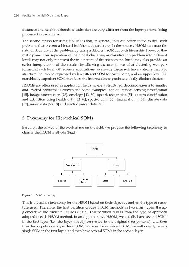
Based on the survey of the work made on the field, we propose the following taxonomy toclassify the HSOM methods (Fig.1).

Figure 1. HSOM taxonomy.

This is a possible taxonomy for the HSOM based on their objective and on the type of struc‐ture used. Therefore, the first partition groups HSOM methods in two main types: the ag‐glomerative and divisive HSOMs (Fig.2). This partition results from the type of approachadopted in each HSOM method. In an agglomerative HSOM, we usually have several SOMsin the first layer (i.e., the layer directly connected to the original data patterns), and thenfuse the outputs in a higher level SOM, while in the divisive HSOM, we will usually have asingle SOM in the first layer, and then have several SOMs in the second layer.


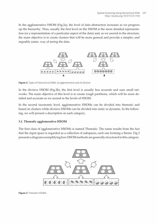
In the agglomerative HSOM (Fig.2a), the level of data abstraction increases as we progressup the hierarchy. Thus, usually the first level on the HSOM is the more detailed representa‐tion (or a representation of a particular aspect of the data) and, as we ascend in the structure,the main objective is to create clusters that will be more general and provide a simpler, andarguably easier, way of seeing the data.

Figure 2. Types of hierarchical SOMs: a) agglomerative and; b) divisive.

In the divisive HSOM (Fig.2b), the first level is usually less accurate and uses small net‐works. The main objective of this level is to create rough partitions, which will be more de‐tailed and accurate as we ascend in the levels of HSOM.

In the second taxonomic level, agglomerative HSOMs can be divided into thematic andbased on clusters while divisive HSOMs can be divided into static or dynamic. In the follow‐ing, we will present a description on each category.

3.1. Thematic agglomerative HSOM

The first class of agglomerative HSOMs is named Thematic. The name results from the factthat the input space is regarded as a collection of subspaces, each one forming a theme. Fig.3presents a diagram exemplifying how HSOM methods are generally structured in this category.

Figure 3. Thematic HSOMs


237

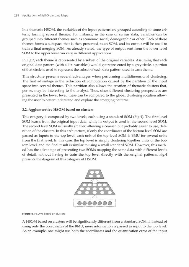
In a thematic HSOM, the variables of the input patterns are grouped according to some cri‐teria, forming several themes. For instance, in the case of census data, variables can begrouped into different themes such as economic, social, demographic or other. Each of thesethemes forms a subspace that is then presented to an SOM, and its output will be used totrain a final merging SOM. As already stated, the type of output sent from the lower levelSOM to the upper level can vary in different applications.

In Fig.3, each theme is represented by a subset of the original variables. Assuming that eachoriginal data pattern (with all its variables) would get represented by a grey circle, a portionof that circle is used to represent the subset of each data pattern used in each theme.

This structure presents several advantages when performing multidimensional clustering.The first advantage is the reduction of computation caused by the partition of the inputspace into several themes. This partition also allows the creation of thematic clusters that,per se, may be interesting to the analyst. Thus, since different clustering perspectives arepresented in the lower level, these can be compared to the global clustering solution allow‐ing the user to better understand and explore the emerging patterns.

3.2. Agglomerative HSOM based on clusters

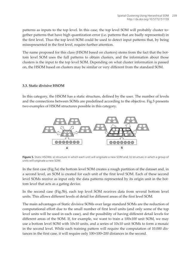
This category is composed by two levels, each using a standard SOM (Fig.4). The first levelSOM learns from the original input data, while its output is used in the second level SOM.The second level SOM is usually smaller, allowing a coarser, but probably easier to use, defi‐nition of the clusters. In this architecture, if only the coordinates of the bottom level SOM arepassed as inputs to the top level, each unit of the top level SOM is BMU for several unitsfrom the first level. In this case, the top level is simply clustering together units of the bot‐tom level, and the final result is similar to using a small standard SOM. However, this meth‐od has the advantage of presenting two SOMs mapping the same data with different levelsof detail, without having to train the top level directly with the original patterns. Fig.4presents the diagram of this category of HSOM.

Figure 4. HSOMs based on clusters

A HSOM based on clusters will be significantly different from a standard SOM if, instead ofusing only the coordinates of the BMU, more information is passed as input to the top level.As an example, one might use both the coordinates and the quantization error of the input


patterns as inputs to the top level. In this case, the top level SOM will probably cluster to‐gether patterns that have high quantization error (i.e. patterns that are badly represented) inthe first level. Thus the top level SOM could be used to detect input patterns that, by beingmisrepresented in the first level, require further attention.

The name proposed for this class (HSOM based on clusters) stems from the fact that the bot‐tom level SOM uses the full patterns to obtain clusters, and the information about thoseclusters is the input to the top level SOM. Depending on what cluster information is passedon, the HSOM based on clusters may be similar or very different from the standard SOM.

3.3. Static divisive HSOM

In this category, the HSOM has a static structure, defined by the user. The number of levelsand the connections between SOMs are predefined according to the objective. Fig.5 presentstwo examples of HSOM structures possible in this category.

Figure 5. Static HSOMs: a) structure in which each unit will originate a new SOM and; b) structure in which a group ofunits will originate a new SOM.

In the first case (Fig.5a) the bottom level SOM creates a rough partition of the dataset and, ina second level, an SOM is created for each unit of the first level SOM. Each of these secondlevel SOMs receive as input only the data patterns represented by its origin unit in the bot‐tom level that acts as a gating device.

In the second case (Fig.5b), each top level SOM receives data from several bottom levelunits. This allows different levels of detail for different areas of the first level SOM.

The main advantages of Static divisive SOMs over large standard SOMs are the reduction ofcomputational effort due to the small number of first level units (and only some of the toplevel units will be used in each case), and the possibility of having different detail levels fordifferent areas of the SOM. If, for example, we want to train a 100x100 unit SOM, we mayuse a bottom level SOM with 10x10 units, and a series of 10x10 unit SOMs to form a mosaicin the second level. While each training pattern will require the computation of 10.000 dis‐tances in the first case, it will require only 100+100=200 distances in the second.


239

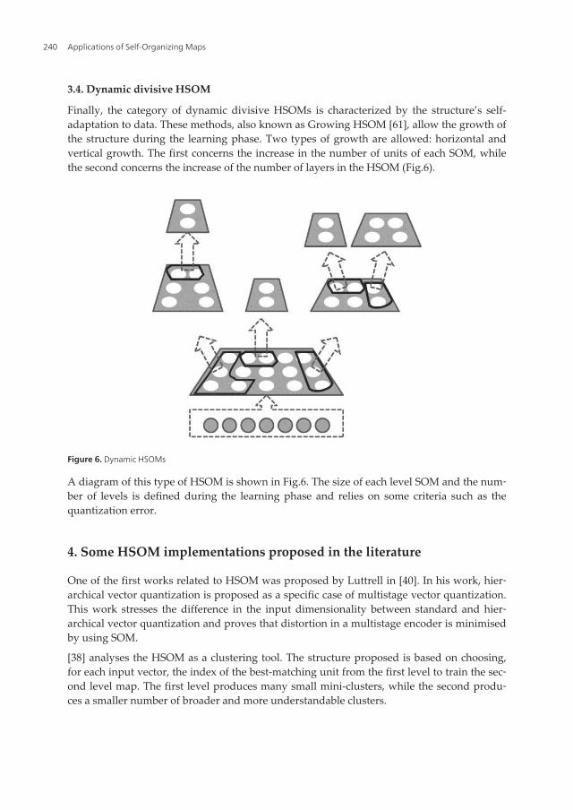
3.4. Dynamic divisive HSOM

Finally, the category of dynamic divisive HSOMs is characterized by the structure’s self-adaptation to data. These methods, also known as Growing HSOM [61], allow the growth ofthe structure during the learning phase. Two types of growth are allowed: horizontal andvertical growth. The first concerns the increase in the number of units of each SOM, whilethe second concerns the increase of the number of layers in the HSOM (Fig.6).

Figure 6. Dynamic HSOMs

A diagram of this type of HSOM is shown in Fig.6. The size of each level SOM and the num‐ber of levels is defined during the learning phase and relies on some criteria such as thequantization error.

4. Some HSOM implementations proposed in the literature

One of the first works related to HSOM was proposed by Luttrell in [40]. In his work, hier‐archical vector quantization is proposed as a specific case of multistage vector quantization.This work stresses the difference in the input dimensionality between standard and hier‐archical vector quantization and proves that distortion in a multistage encoder is minimisedby using SOM.

[38] analyses the HSOM as a clustering tool. The structure proposed is based on choosing,for each input vector, the index of the best-matching unit from the first level to train the sec‐ond level map. The first level produces many small mini-clusters, while the second produ‐ces a smaller number of broader and more understandable clusters.


HSOM has proved to be quite valuable for processing temporal data, often using differenttime scales at different hierarchical levels. An example is the work of [58, 60], where theauthors use HSOM to perform sequence classification and discrimination in musical andelectric power load data. Another example is [62] where HSOM is used to process sleepapnea data.

Another class of HSOM is proposed in [61]with the Growing Hierarchical Self-OrganizingMap (GHSOM). This neural network model is composed of several SOMs, each of which isallowed to grow vertically and horizontally. During the training process, until a given crite‐rion is met, each SOM is allowed to grow in size (horizontal growth) and the number of lay‐ers is allowed to grow (vertical growth) to form a layered architecture such that relationsbetween input data patterns are further detailed at higher levels of the structure. One of theproblems of GHSOM is the definition of the two thresholds used to control the two types ofgrowth. Several authors proposed some variants to this method to better define these crite‐ria. One example is the Enrich-GHSOM [50]. Its main difference is the possibility to force thegrowth of the hierarchy along some predefined paths. This model classifies data into a pre-defined taxonomic structure. Another example of a GHSOM variant is the RoFlex-HSOMextension [57]. This method is suited to non-stationary time-dependent environments by in‐corporating robustness and flexibility in the incremental learning algorithm. RoFlex-HSOMexhibits plasticity when finding the structure of the data, and gradually forgets (but not cat‐astrophically) previous learned patterns. Also,[63] proposed a Tension and Mapping Ratioextension (TMR) to the GHSOM. Two new indexes are introduced, the mapping ratio (MR)and the tension (T) that will control the growth of the GHSOM. MR measures the ratio ofinput patterns that get better represented by a virtual unit, placed between two existentunits. T measures how similar are the distances between all the units.

Another example of HSOM is proposed in [64] with the Hierarchical Overlapped SOM (HO‐SOM). The process starts by using just one SOM. After completing the unsupervised learn‐ing, each unit is labelled. Then, a supervised learning method is used (LVQ2) and units aremerged or removed, based on the number of mapped patterns. After this, a new LVQ2 isapplied and, based on the classification quality, additional layers can be created. The processis then repeated for each of these layers.

A similar structure is presented in [65], which proposes a cooperative learning algorithm forthe hierarchical SOM. In the first layer, some BMUs are selected, and for each of these BMUsa SOM in the second layer is created. Input patterns used in this second level SOM are de‐rived from the original BMU.

Ichiki et al.[43] propose a hierarchical SOM do deal with semantic maps. In this proposal,each input pattern is composed by two parts: the attribute and the symbol,X i = X ai X si .Theattribute partX aiis composed by the variables describing the input pattern, while the symbolpartX si is a binary vector. The first level SOM is trained using both parts of the patterns,while the second level SOM only uses the symbol set and information from the first level.

HSOM has also been used for phoneme recognition [51]. The authors use sound signal at‐tributes in a first level SOM to classify the phonemes into pause, vocalised phoneme, non-


241

vocalised phoneme, and fricative segment. After phonemes are classified, a featurefrequency-scale vector is used to train the corresponding second level SOM.

A different approach called tree structured topological feature map (TSTFM) is presented in[37]. This approach uses a hierarchical structure to search for the BMU, thus reducing com‐putation times. While the purpose of this approach is strictly to reduce computation times,its tree searching strategy is in effect a series of static divisive HSOMs.

Miikkulainen [41] proposes a hierarchical feature map to recognize an input story (text) asan instance of a particular script by classifying it in three levels: scripts, tracks and role bind‐ings. At the lowest level, a standard SOM is used for a gross classification of the scripts. Thesecond level SOMs receives only the input patterns relative to its scripts, and different tracksare classified at this level. Finally, in the third level a role classification is made.

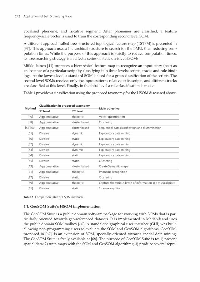
Table 1 provides a classification using the proposed taxonomy for the HSOM discussed above.

MethodClassification in proposed taxonomy

Main objective1st level 2nd level

[40] Agglomerative thematic Vector quantization

[38] Agglomerative cluster based Clustering

[58][60] Agglomerative cluster based Sequential data classification and discrimination

[61] Divisive dynamic Exploratory data mining

[50] Divisive static Exploratory data mining



[64] Divisive static Exploratory data mining

[65] Divisive static Clustering

[43] Agglomerative cluster based Create Semantic maps

[51] Agglomerative thematic Phoneme recognition

[37] Divisive static Clustering

[59] Agglomerative thematic Capture the various levels of information in a musical piece

[41] Divisive static Story recognition

Table 1. Comparison table of HSOM methods

4.1. GeoSOM Suite’s HSOM implementation

The GeoSOM Suite is a public domain software package for working with SOMs that is par‐ticularly oriented towards geo-referenced datasets. It is implemented in Matlab® and usesthe public domain SOM toolbox [66]. A standalone graphical user interface (GUI) was built,allowing non-programming users to evaluate the SOM and GeoSOM algorithms. GeoSOM,proposed in [67], is an extension of SOM, specially oriented towards spatial data mining.The GeoSOM Suite is freely available at [68]. The purpose of GeoSOM Suite is to: 1) presentspatial data; 2) train maps with the SOM and GeoSOM algorithms; 3) produce several repre‐


sentations (views) of the data and; 4) establish dynamic links between views, allowing aninteractive exploration of the data.

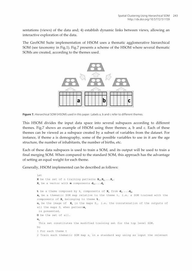
The GeoSOM Suite implementation of HSOM uses a thematic agglomerative hierarchicalSOM (see taxonomy in Fig.1). Fig.7 presents a scheme of the HSOM where several thematicSOMs are created, according to the themes used.

Figure 7. Hierarchical SOM (HSOM) used in this paper. Labels a, b and c refer to different themes.

This HSOM divides the input data space into several subspaces according to differentthemes. Fig.7 shows an example of HSOM using three themes: a, b and c. Each of thesethemes can be viewed as a subspace created by a subset of variables from the dataset. Forinstance, if theme a is demography, some of the possible variables to use in it are the agestructure, the number of inhabitants, the number of births, etc.

Each of these data subspaces is used to train a SOM, and its output will be used to train afinal merging SOM. When compared to the standard SOM, this approach has the advantageof setting an equal weight for each theme.

Generally, HSOM implemented can be described as follows:

Let

X be the set of n training patterns X1,X2,...Xn.

Xi be a vector with m components d1,...dm

t be a theme composed by kt components of Xi from d1,...dktst be a thematic SOM map relative to the theme t, i.e. a SOM trained with the

components of Xi belonging to theme t.

oi be the image of Xi in the maps St, i.e. the concatenation of the outputs of

all the maps St when patternxi is presented.

O be the set of all.

oi This set constitutes the modified training set for the top level SOM.

Do

1 For each theme t

2 Train each thematic SOM map st in a standard way using as input the relevant


243

components of X

3 Create the set of modified training patterns O as a concatenation of the pos-

sible outputs of maps St, using for each input pattern:

a. The coordinates of its BMU.

b. Its quantization error.

c. Its distance to each unit(i.e., all quantization errors).

4 Train the top level SOM using as input the set of modified training patterns

O.

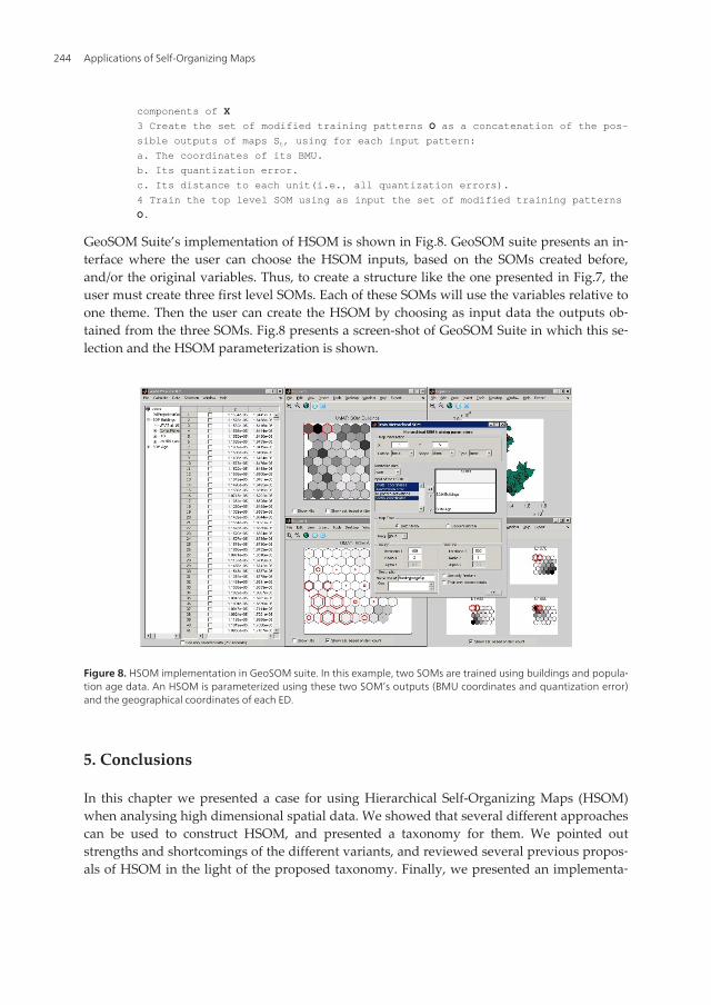
GeoSOM Suite’s implementation of HSOM is shown in Fig.8. GeoSOM suite presents an in‐terface where the user can choose the HSOM inputs, based on the SOMs created before,and/or the original variables. Thus, to create a structure like the one presented in Fig.7, theuser must create three first level SOMs. Each of these SOMs will use the variables relative toone theme. Then the user can create the HSOM by choosing as input data the outputs ob‐tained from the three SOMs. Fig.8 presents a screen-shot of GeoSOM Suite in which this se‐lection and the HSOM parameterization is shown.

Figure 8. HSOM implementation in GeoSOM suite. In this example, two SOMs are trained using buildings and popula‐tion age data. An HSOM is parameterized using these two SOM’s outputs (BMU coordinates and quantization error)and the geographical coordinates of each ED.

5. Conclusions

In this chapter we presented a case for using Hierarchical Self-Organizing Maps (HSOM)when analysing high dimensional spatial data. We showed that several different approachescan be used to construct HSOM, and presented a taxonomy for them. We pointed outstrengths and shortcomings of the different variants, and reviewed several previous propos‐als of HSOM in the light of the proposed taxonomy. Finally, we presented an implementa‐


tion of a HSOM that is particularly well suited for spatial analysis. This implementation ispublically available for general use at [68].

Author details

Roberto Henriques1*, Victor Lobo1,2 and Fernando Bação1

*Address all correspondence to: [email protected]

1 ISEGI, Universidade Nova de Lisboa Campolide, Portugal

2 CINAV, PO Navy Research Center, Alfeite, Portugal

References

[1] Openshaw, S., & Openshaw, C. (1997). Artificial Intelligence in Geography, John Wiley& Sons, Inc., 329.

[2] Gahegan, M. (2003). Is inductive machine learning just another wild goose (or mightit lay the golden egg)? International Journal of Geographical Information Science, 17(1),69-92.

[3] Miller, H., & Han, J. (2001). Geographic Data Mining and Knowledge Discovery.London, UK, Taylor and Francis., 372.

[4] Openshaw, S. (1994). What is GISable spatial analysis? in New Tools for Spatial Anal‐ysis Eurostat Luxembourg , 36-44.

[5] Jain, A. K., Murty, M. N., & Flynn, P. J. (1999). Data clustering: a review., ACM Comput.Surv, 31(3), 264-323.

[6] Fayyad, U. M., Piatetsky-Shapiro, G., & Smyth, P. (1996). From Data Mining toKnowledge Discovery: An Overview. , in Advances in Knowledge Discovery andData Mining, U.M. Fayyad, et al., Editors., AAAI Press/ The MIT Press. , 1-43.

[7] Miller, H., & Han, J. (2001). Geographic data mining and knowledge discovery anoverview. , in Geographic Data Mining and Knowledge Discovery, H. Miller and J.Han, Editors., Taylor and Francis London, UK , 3-32.

[8] Fukunaga, K. (1990). Introduction to statistical pattern recognition. nd ed: AcademicPress Inc.

[9] Duda, R. O., Hart, P. E., & Stork, D. G. (2001). Pattern Classification, Wiley-Inter‐science.


245

[10] Kaufman, L., & Rousseeuw, P. J. (1990). Finding groups in data : an introduction tocluster analysis. Wiley series in probability and mathematical statistics. Appliedprobability and statistics , New York John Wiley & Sons ., 342.

[11] Han, J., Kamber, M., & Tung, A. K. H. (2001). Spatial clustering methods in data min‐ing: A survey, in Geographic Data Mining and Knowledge Discovery. H.J. Miller andJ. Han, Editors., Taylor and Francis London. , 188-217.

[12] Plane, D. A., & Rogerson, P. A. (1994). The Geographical Analysis of Population:With Applications to Planning and Business,. New York, John Wiley & Sons.

[13] Feng, Z., & Flowerdew, R. (1998). Fuzzy geodemographics: a contribution from fuzzyclustering methods,. in Innovations in GIS 5, S. Carver, Editor, Taylor & Francis Lon‐don , 119-127.

[14] Birkin, M., & Clarke, G. (1998). GIS, geodemographics and spatial modeling in theUK financial service industry. Journal of Housing Research, 9, 87-111.

[15] Openshaw, S., Blake, M., & Wymer, C. (1995). Using Neurocomputing Methods toClassify Britain’s Residential Areas Available from: http://www.geog.leeds.ac.uk/papers/95-1/.

[16] Openshaw, S., & Wymer, C. (1995). . Classifying and regionalizing census data, inCensus users handbook,. S. Openshaw, Editor, GeoInformation International Cam‐brige, UK , 239-268.

[17] Fahmy, E., Gordon, D., & Cemlyn, S. (2002). Poverty and Neighbourhood Renewal inWest Cornwall. in Social Policy Association Annual Conference Nottingham, UK.

[18] Birkin, M., Clarke, G., & Clarke, M. (1999). GIS for Business and Service Planning, inGeographical Information Systems. , M. Goodchild, et al., Editors.,GeoinformationCambridge

[19] Bellman, R. (1961). Adaptive Control Processes: A Guided Tour,. Princeton, New Jer‐sey, Princeton University Press.

[20] Rees, P., Martin, D., & Williamson, P. (2002). Census data resources in the UnitedKingdom, in. The Census Data System, P. Rees, D. Martin, and P. Williamson, Edi‐tors., Wiley Chichester , 1-24.

[21] Goodchild, M. (1986). Spatial Autocorrelation. CATMOG, 47, Norwich, Geo Books.

[22] Tobler, W. (1973). A continuous transformation useful for districting. Annals, NewYork Academy of Sciences, 219, 215-220.

[23] Openshaw, S. (1984). The modifiable areal unit problem. Norwich, England, Geo‐Books- CATMOG 38.

[24] Kohonen, T. (2001). Self-Organizing Maps. rd edition ed, Berlin Springer

[25] Muñoz, A., & Muruzábal, J. (1998). Self-organizing maps for outlier detection. Neuro‐computing, 18(1-3), 33-60.


[26] Hadzic, F., Dillon, T. S., & Tan, H. (2007). Outlier detection strategy using the self-organizing map. in Knowledge Discovery and Data Mining: Challenges and Reali‐ties, X.Z.I. Davidson, Editor, Information Science Reference Hershey, PA, USA ,224-243.

[27] Nag, A., Mitra, A., & Mitra, S. (2005). Multiple outlier detection in multivariate datausing self-organizing maps title. Computational Statistics, 245-264.

[28] Barbalho, J. M., et al. (2001). Hierarchical SOM applied to image compression. in In‐ternational Joint Conference on Neural Networks,. IJCNN’01. 2001. Washington, DC

[29] Céréghino, R., et al. (2005). Using self-organizing maps to investigate spatial patternsof non-native species. Biological Conservation, 459-465.

[30] Green, C., et al. (2003). Geographic analysis of diabetes prevalence in an urban area.Social Science & Medicine, 57(3), 551-560.

[31] Guo, D., Peuquet, D. J., & Gahegan, M. (2003). ICEAGE: Interactive Clustering andExploration of Large and High-Dimensional Geodata. GeoInformatica, 229-253.

[32] Koua, E., & Kraak, M. J. (2004). Geovisualization to support the exploration of largehealth and demographic survey data. International Journal of Health Geographics, 3(1),12.

[33] Oyana, T. J., et al. (2005). Exploration of geographic information systems (GIS)-basedmedical databases with self-organizing maps (SOM): A case study of adult asthma.in Proceedings of the 8th International Conference on GeoComputation Ann ArborUniversity of Michigan

[34] Skupin, A. (2003). A novel map projection using an artificial neural network. in Pro‐ceedings of 21st International Cartographic Conference Durban, South Africa: ICC.

[35] Bação, F., Lobo, V., & Painho, M. (2008). Applications of Different Self-OrganizingMap Variants to Geographical Information Science Problems. in Self-OrganisingMaps: Applications in Geographic Information Science P. Agarwal and A. Skupin,Editors. , 21-44.

[36] Kohonen, T. (1982). Self-organized formation of topologically correct feature maps.Biological Cybernetics, 59-69.

[37] Koikkalainen, P., & Oja, E. (1990). Self-organizing hierarchical feature maps. in Inter‐national Joint Conference on Neural Networks, IJCNN Washington, DC, USA

[38] Lampinen, J., & Oja, E. (1992). Clustering properties of hierarchical self-organizingmaps. Journal of Mathematical Imaging and Vision, 261-272.

[39] Kemke, C., & Wichert, A. (1993). Hierarchical Self-Organizing Feature Maps forSpeech Recognition. in Proc. WCNN’93, World Congress on Neural Networks Law‐rence Erlbaum.


247

[40] Luttrell, S. P. (1989). Hierarchical vector quantisation. Communications, Speech and Vi‐sion, IEE Proceedings I, 136(6), 405-413.

[41] Miikkulainen, R. (1990). Script Recognition with Hierarchical Feature Maps. Connec‐tion Science, 2(1), 83-101.

[42] Luttrell, S. P. (1988). Self-organising multilayer topographic mappings. in IEEE Inter‐national Conference on Neural Networks San Diego, California

[43] Ichiki, H., Hagiwara, M., & Nakagawa, M. (1991). Self-organizing multilayer seman‐tic maps. in International Joint Conference on Neural Networks, IJCNN-91. Seattle.

[44] Graham, D. P. W., & D’Eleuterio, G. M. T. (1991). A hierarchy of self-organized mul‐tiresolution artificial neural networks for robotic control. in International Joint Con‐ference on Neural Networks, IJCNN-91. Seattle.

[45] Lee, J., & Ersoy, O. K. (2005). Classification of remote sensing data by multistage self-organizing maps with rejection schemes. in Proceedings of 2nd International Confer‐ence on Recent Advances in Space Technologies, RAST 2005.Istanbul, Turkey

[46] Li, J. M., & Constantine, N. (1989). Multistage vector quantization based on the self-organization feature maps. in Visual Communications and Image ProcessingIV..SPIE

[47] Saavedra, C., et al. (2007). Fusion of Self Organizing Maps. in Computational andAmbient Intelligence , 227-234.

[48] Sauvage, V. (1997). The T-SOM (Tree-SOM). in Advanced Topics in Artificial Intelli‐gence , 389-397.

[49] Bação, F., Lobo, V., & Painho, M. (2005). Geo-SOM and its integration with geograph‐ic information systems. , in WSOM 05, 5th Workshop On Self-Organizing Maps: Uni‐versity Paris 1 Panthéon-Sorbonne , 5-8.

[50] Chifu, E. S., & Letia, I. A. (2008). Text-Based Ontology Enrichment Using Hierarchi‐cal Self-organizing Maps. in Nature inspired Reasoning for the Semantic Web (Na‐tuReS 2008) Karlsruhe, Germany.

[51] Kasabov, N., & Peev, E. (1994). Phoneme Recognition with Hierarchical Self Organ‐ised Neural Networks and Fuzzy Systems- A Case Study. in Proc. ICANN’94, Int.Conf. on Artificial Neural Networks Springer

[52] Douzono, H., et al. (2002). A design method of DNA chips using hierarchical self-or‐ganizing maps. in Proceedings of the 9th International Conference on Neural Infor‐mation Processing. ICONIP’02. Orchid Country Club, Singapore

[53] Hanke, J., et al. (1996). Self-organizing hierarchic networks for pattern recognition inprotein sequence. Protein Science, 5(1), 72-82.

[54] Zheng, C., et al. (2007). Hierarchical SOMs: Segmentation of Cell-Migration Images.in Advances in Neural Networks- ISNN 2007 , 938-946.


[55] Vallejo, E., Cody, M., & Taylor, C. (2007). Unsupervised Acoustic Classification ofBird Species Using Hierarchical Self-organizing Maps. in Progress in Artificial Life ,212-221.

[56] Tsao, C. Y., & Chou, C. H. (2008). Discovering Intraday Price Patterns by Using Hier‐archical Self-Organizing Maps. in JCIS-2008 Proceedings, Advances in IntelligentSystems Research.. Shenzhen, China Atlantis Press

[57] Salas, R., et al. (2007). A robust and flexible model of hierarchical self-organizingmaps for non-stationary environments. Neurocomput, 70(16-18), 2744-2757.

[58] Carpinteiro, O. A. S. (1999). A Hierarchical Self-Organizing Map Model for SequenceRecognition. Neural Processing Letters, 9(3), 209-220.

[59] Law, E., & Phon-Amnuaisuk, S. (2008). Towards Music Fitness Evaluation with theHierarchical SOM. in Applications of Evolutionary Computing , 443-452.

[60] Carpinteiro, O.A.S., & Alves da Silva, A.P. (2001). A Hierarchical Self-OrganizingMap Model in Short-Term Load Forecasting. Journal of Intelligent and Robotic Systems,105-113.

[61] Dittenbach, M., Merkl, D., & Rauber, A. (2002). Organizing And Exploring High-Di‐mensional Data With The Growing Hierarchical Self-Organizing Map. in Proceed‐ings of the 1st International Conference on Fuzzy Systems and Knowledge Discovery(FSKD 2002) Orchid Country Club, Singapore.

[62] Guimarães, G., & Urfer, W. (2000). Self-Organizing Maps and its Applications inSleep Apnea Research and Molecular Genetics,. , University of Dortmund- StatisticsDepartment

[63] Pampalk, E., Widmer, G., & Chan, A. (2004). A new approach to hierarchical cluster‐ing and structuring of data with Self-Organizing Maps. Intell. Data Anal, 8(2),131-149.

[64] Suganthan, P. N. (1999). Hierarchical overlapped SOM’s for pattern classification.Neural Networks, IEEE Transactions on, 10(1), 193-196.

[65] Endo, M., Ueno, M., & Tanabe, T. (2002). A Clustering Method Using HierarchicalSelf-Organizing Maps. The Journal of VLSI Signal Processing, 32(1), 105-118.

[66] Vesanto, J., et al. (1999). Self-organizing map in Matlab: the SOM Toolbox. in Pro‐ceedings of the Matlab DSP Conference Espoo, Finland: Comsol Oy

[67] Bação, F., Lobo, V., & Painho, M. (2004). Geo-self-organizing map (Geo-SOM) forbuilding and exploring homogeneous regions. Geographic Information Science, Proceed‐ings, 3234, 22-37.

[68] Lobo, V., Bação, F., & Henriques, R. (2009). GeoSOM suite. 15-11-2009]; Availablefrom: www.isegi.unl.pt/labnt/geosom


249

Spatial Clustering Using Hierarchical SOM -...

Documents

Transcript of Spatial Clustering Using Hierarchical SOM -...