Spatial and multi-temporal weed mapping at early stage of cotton crop using GIS

Kalivas D.P., G. Economou and Vlachos C.E. 

Athens 2009

AGRICULTURAL UNIVERSITY OF ATHENSAGRICULTURAL UNIVERSITY OF ATHENS

General Scope

Spatial mapping of weeds in one of the most important cotton cultivation area in Greece

Creation of a Geographical database

Influence of abiotic factors and cultivation techniques on weed appearance

Questions ?

Is there a weed problem

Which weeds are the most prevalent during the crucial stages of the crop

Are there any new weeds Is pre- emergence control effective

Would a geographical database be helpful in taking decision

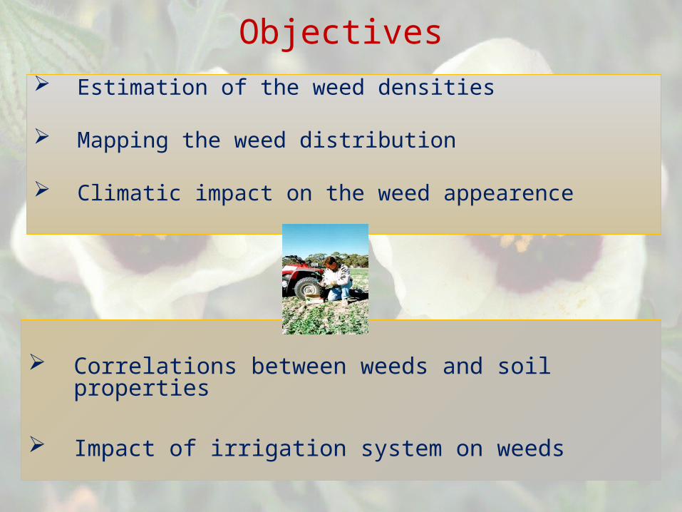
Estimation of the weed densities

Mapping the weed distribution

Climatic impact on the weed appearence

Correlations between weeds and soil properties

Impact of irrigation system on weeds

Objectives

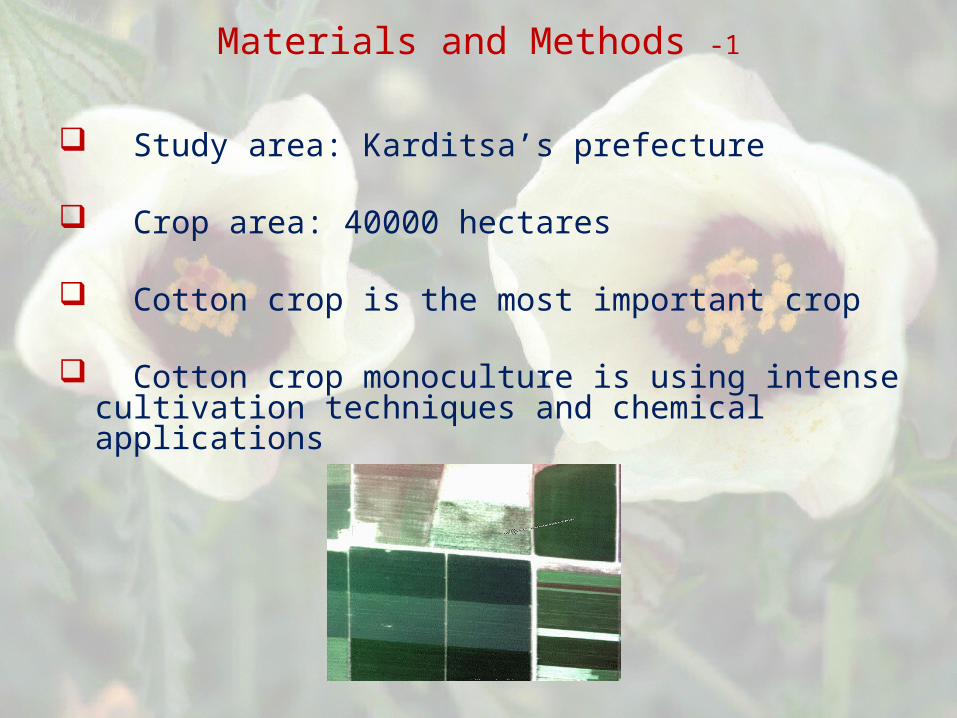
Study area: Karditsa’s prefecture Crop area: 40000 hectares

Cotton crop is the most important crop

Cotton crop monoculture is using intense cultivation techniques and chemical applications

Materials and Methods -1

Materials and Methods -2

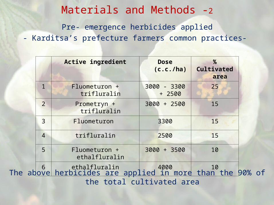
Pre- emergence herbicides applied- Karditsa’s prefecture farmers common practices-

  Active ingredient Dose (c.c./ha)

%Cultivated

area

1 Fluometuron + trifluralin 3000 - 3300 + 2500

25

2 Prometryn + trifluralin 3000 + 2500 15

3 Fluometuron 3300 15

4 trifluralin 2500 15

5 Fluometuron + ethalfluralin

3000 + 3500 10

6 ethalfluralin 4000 10

The above herbicides are applied in more than the 90% of the total cultivated area

Materials and methods -3

Time of sampling: 2 cultivation periods (2007, 2008)(Before the first mechanical weed control)

Crop stage: Pre- anthesis stage

Grid sapmling scheme: cell size 2,6*2,6km

183 cells were designed only above the cultivated area (lowland)

1 sampling per cell

Final number of samplings: 101 (2007), 80 (2008)

Materials and methods -4

Grid applied over the hole prefecture

Cell size: 2,6 km x 2,6 km

Spatial distribution of the sampling sites

Karditsa

Materials and methods -5

In each sampling site we sampled 5 different points (each point was 5 m2) Samplings took place between rows

The distance between the points was 3 meters.

Coordinates were recorded from the central point of each area

Geographical Database(Using the software GIS ArcMap v. 9.3)

 

Weed density per species Total number of weeds per m2

Irrigation system

(sprinkler and drip) Soil properties (texture, calcium carbonates) Climatic data, 2 meteorological stations (precipitation, temperature ) Coordinates

Information input were based on descriptive data

Materials and methods -6

Transformed in GIS layers

Data collected per sampling site

Methods of analysis

Non spatial: Univariate analysis: mean, standard deviation, standard error

of mean

Bivariate analysis: - correlation coefficient (Pearson correlation coefficient),

- comparisons of means (Τ-test) and - analysis of variance (one -way)

Spatial: Examination of the weed spatial distribution and creation of weed appearance interpolated maps (using Inverse Distance Weighting method)

Materials and methods -7

2007 Meteorological Data

Results- climatic

Karditsa stationMean air temperature 17,5ο CTotal rainfall 530 mm

Dafnospilia stationMean air temperature 16,4ο CTotal rainfall 646 mm

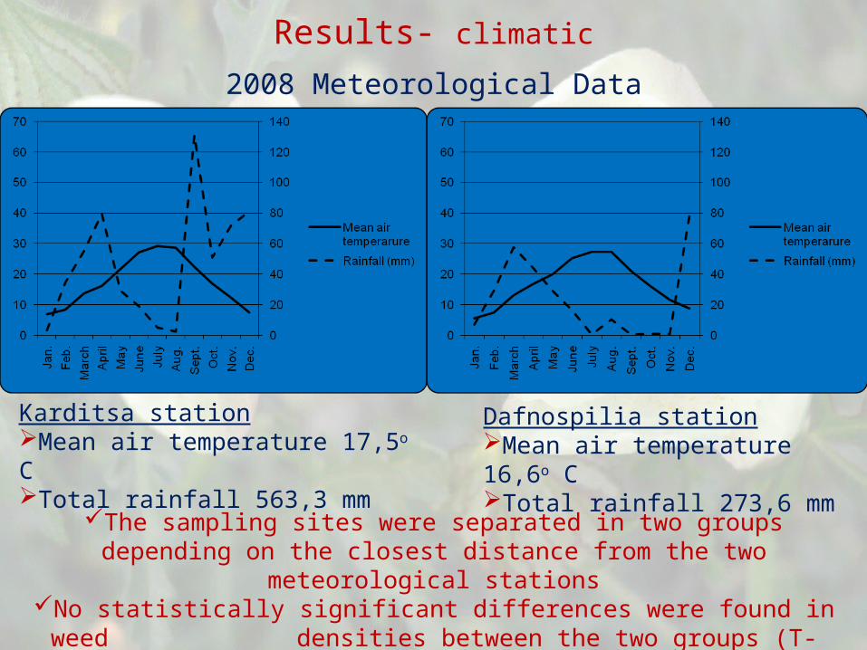
Results- climatic

2008 Meteorological Data

Karditsa stationMean air temperature 17,5ο CTotal rainfall 563,3 mm

Dafnospilia stationMean air temperature 16,6ο CTotal rainfall 273,6 mm

The sampling sites were separated in two groups depending on the closest distance from the two meteorological stations

No statistically significant differences were found in weed densities between the two groups (T-test)

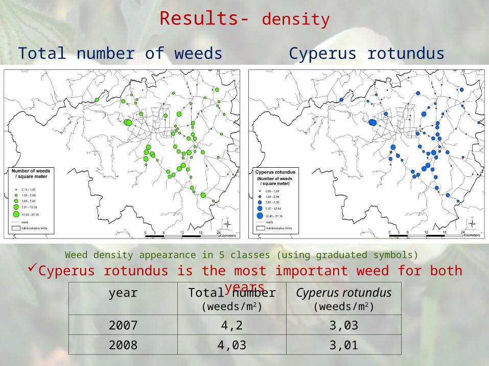
Results- density

Cyperus rotundus is the most important weed for both years

Total number of weeds Cyperus rotundus

Weed density appearance in 5 classes (using graduated symbols)

year Total number (weeds/m2)

Cyperus rotundus(weeds/m2)

2007 4,2 3,03

2008 4,03 3,01

Results- density

2007 2008

   Scientific names

Mean of weed

s( per

m2)

 Scientific names

Mean of weeds

( per m2)

1 Cyperus rotundus 3,036 1 Cyperus rotundus 3,016

2 Convolvulus arvensis 0,349 2 Portulaca oleracea 0,257

3 Portulaca oleracea 0,190 3 Convolvulus arvensis 0,203

4 Cynodon dactylon 0,181 4 Cynodon dactylon 0,183

5 Sorghum halepense 0,103 56789

1011121314151617

Solanum nigrumEchinochloa crus-galliDigitaria sanguinalisSorghum halepense

Chrozophora tinctoriaAmaranthus retroflexusAmaranthus blitoidesAbutilon theophrasti

Hibiscus trionumXanthium strumariumSolanum eleagnifolium

Datura stramoniumSetaria viridis

<0,1

67891

01

11

21

31

4

Xanthium strumariumSolanum nigrum

Amaranthus retroflexus

Chrozophora tinctoriaDatura stramonium

Echinochloa crus-galliHibiscus trionum

Amaranthus blitoidesAbutilon theophrasti

< 0,1

Ranking of the weeds based on density (2007,2008)

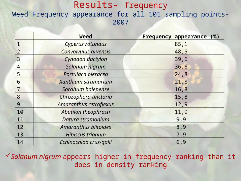
Weed Frequency appearance (%)1 Cyperus rotundus 85,12 Convolvulus arvensis 48,53 Cynodon dactylon 39,64 Solanum nigrum 36,65 Portulaca oleracea 24,86 Xanthium strumarium 21,87 Sorghum halepense 16,88 Chrozophora tinctoria 15,89 Amaranthus retroflexus 12,910 Abutilon theophrasti 11,911 Datura stramonium 9,912 Amaranthus blitoides 8,913 Hibiscus trionum 7,914 Echinochloa crus-galli 6,9

Results- frequencyWeed Frequency appearance for all 101 sampling points- 2007

Solanum nigrum appears higher in frequency ranking than it does in density ranking

Results- frequencyWeed Frequency appearance for all 80 sampling points- 2008

Weed Frequency appearance (%)1 Cyperus rotundus 82,5

2 Convolvulus arvensis 43,8

3 Cynodon dactylon 31,3

4 Solanum nigrum 22,5

5 Portulaca oleracea 20,0

6 Sorghum halepense 12,5

7 Chrozophora tinctoria 11,3

8 Xanthium strumarium 10,0

9 Amaranthus blitoides 8,8

10 Datura stramonium 6,3

11 Abutilon theophrasti 6,3

12 Amaranthus retroflexus 5,0

13 Hibiscus trionum 3,8

14 Digitaria sanguinalis 3,8

15 Echinochloa crus-galli 3,8

16 Setaria viridis 1,3

17 Solanum eleagnifolium 1,3

The first five weeds appear in the same position for both years

Results- spatial distribution

In both years the highest values, appear on the southwestern part of the area

In 2008 the spatial distribution of the high values are more uniform

Total number of weeds(Map of continuous distribution using inverse distance weighing

method)

2007 2008

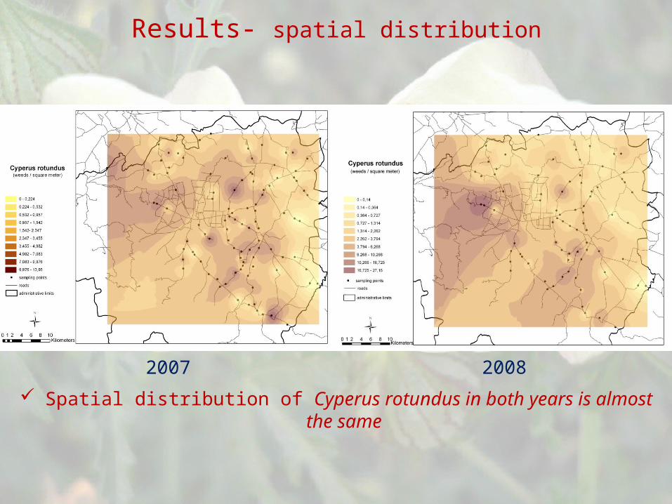
Results- spatial distribution

Spatial distribution of Cyperus rotundus in both years is almost the same

2007 2008

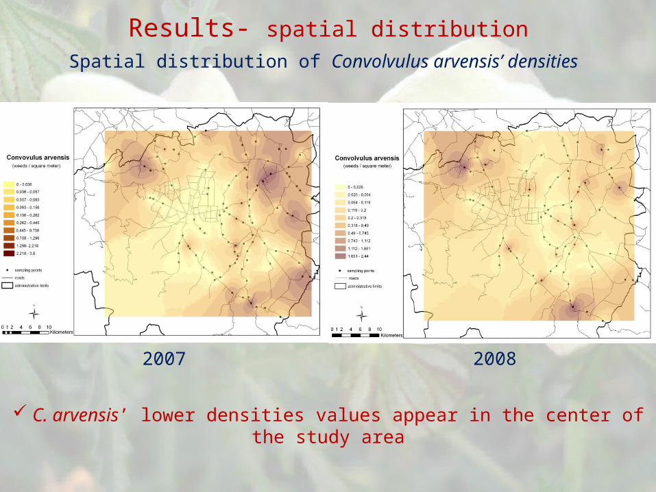
Results- spatial distributionSpatial distribution of Convolvulus arvensis’ densities

2007 2008

C. arvensis’ lower densities values appear in the center of the study area

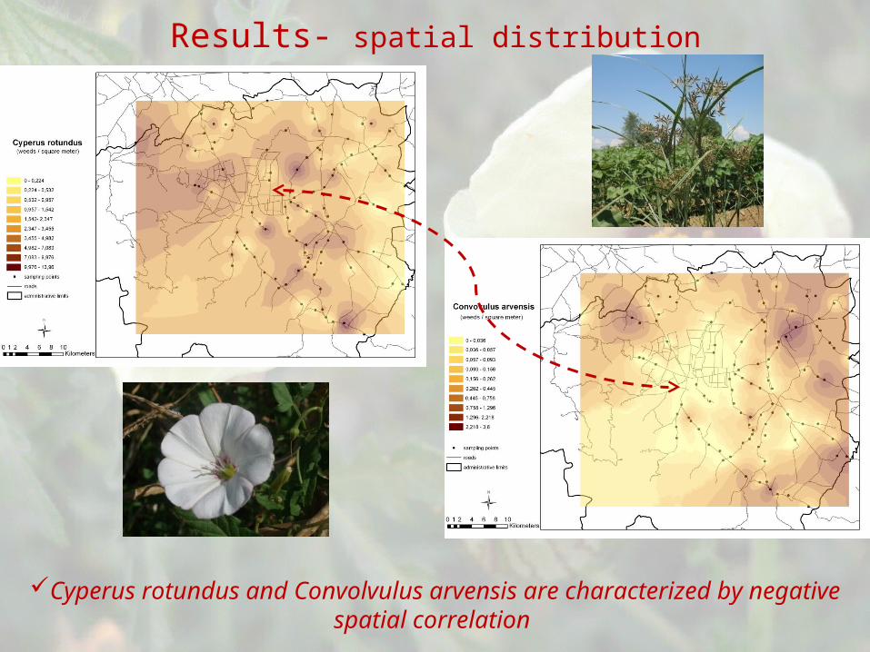
Results- spatial distribution

Cyperus rotundus and Convolvulus arvensis are characterized by negative spatial correlation

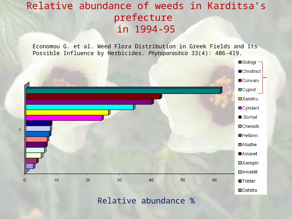
Relative abundance of weeds in Karditsa’s prefecture in 1994-95

Relative abundance %

Economou G. et al. Weed Flora Distribution in Greek Fields and Its Possible Influence by Herbicides. Phytoparasitica 33(4): 406-419.

2007Sprinkler irr.- Mean: 4,64 weeds/ m2

(74 irrigated sampling sites)Drip irr.- Mean: 2,99 weeds/ m2

(27 irrigated sampling points)

Results- irrigation2008

Sprinkler irr.- Mean: 4,5 weeds/ m2

(51 irrigated sampling sites)

Drip irr.- Mean: 3,19 weeds/ m2 (29 irrigated sampling points)

Irrigation effect on the density of the most common weeds

Statistically significant differences, for 2007:• Cyperus rotundus

3,32 plants/ m2 (sprinkler irrig.) – 2,23 plants/ m2 (drip irrig.)

• Convolvulus arvensis0,42 plants/ m2 (sprinkler irrig.) – 0,14 plants/ m2 (drip irrig.)

Results- irrigation

Statistically significant differences, for 2008:• Cyperus rotundus

3,58 plants/ m2 (sprinkler irrig.) – 2 plants/ m2 (drip irrig.)

• Convolvulus arvensis0,25 plants/ m2 (sprinkler irrig.) – 0,11 plants/ m2 (drip irrig.)

Soil properties effect on the weed densities

Texture Class

Sampling points

Mean of weeds

Si, SiL, FSL, L 42 0,1986

SCL, CL,SiCL 37 0,1881

SC, SiC, C 22 0,9

Total 101 0,348

Results- soil properties

Reaction with HCL Sampling points

Mean of weeds

no reaction throughout the surface profile 38 0,249

some reaction occurs deeper than 25 cm 32 0,018

indicates slight reaction in the surface layer

(0-25cm) 15 0,693

strong reaction in the surface layer (0-25cm) 16 0,6

Total 101 0,348

Mean of C. arvensis plants per m2, for each class of soil texture

Mean of C. arvensis plants per m2, for each class of CaCO3 content

All differences are statistically significant (p=0,05)

Correlations between weed species and between weed species and soil properties

Results- correlations

2007 2008

    C.C p- value C.C p- value

Cyperus rotundus Convolvulus arvensis -0,27 0,006 -0,19 0,08Convolvulus

arvensis Soil texture (% clay) 0,33 0,001 0,15 0,19

>> Carbonates content 0,217 0,029 0,17 0,12

Cyperus rotundusTotal density of

weeds 0,921 0,000 0,925 0,000

Cynodon dactylon Cyperus rotundus -0,211 0,034 -0,15 0,18

c.c. Correlation coefficient

Cyperus rotundus is negatively correlated with Convolvulus arvensisConvolvulus arvensis is positively correlated with both soil

propertiesCyperus rotundus is positively correlated with the total density of

weedsCynodon dactylon is negatively correlated with Cyperus rotundus

Conclusions

1. Development of a database regarding the appearance of the weeds and the soil parameters in Karditsa’s prefecture cultivation zone using GIS

2. Mapping the most important weeds (Cyperus rotundus)

3. The most important perennial weeds of the area are Cyperus rotundus, Convolvulus arvensis, Cynodon dactylon

4. The most important annual weed was Portulaca oleracea

5. Drip irrigation constitutes a method of side weed control

6. Convolvulus arvensis responses in high carbonate content and in high clay content

7. The two major perennial weeds (Cyperus rotundus and Convolvulus arvensis) of the area, seem to appear in different places, proving a negative spatial relationship

8. Perennial weeds are difficult to control

9. Comparing the results to the respective ones taken in 1994 we observe that the annual weeds are no longer a serious problem for the farmers. Control of annual weeds proves to be effective

Conclusions

10. Comparing our results with the previous ones of 1994-95, no new species were recorded

11. 2007 results were very similar to 2008 results regarding the spatial distribution of the main weeds, the density and frequency of the main weeds, and the overall density

Conclusions

Finally with the developedGeographical database

It is easier to: Monitor the weed appearance in regards to

abiotic factors and change of land use Map the problematic areas (Appearance of new weed species-

Development of Resistance)