Sparsity-promoting Bayesian inversion · Promoting sparsity using Besov space priors ... Saksman &...
73
Sparsity-promoting Bayesian inversion Samuli Siltanen Department of Mathematics and Statistics University of Helsinki Inverse Problems and Optimal Control for PDEs University of Warwick, May 23–27, 2011
Transcript of Sparsity-promoting Bayesian inversion · Promoting sparsity using Besov space priors ... Saksman &...
Sparsity-promoting Bayesian inversion
Samuli Siltanen
Department of Mathematics and StatisticsUniversity of Helsinki
Inverse Problems and Optimal Control for PDEsUniversity of Warwick, May 23–27, 2011

This is a joint work with
Ville Kolehmainen, University of Eastern Finland
Matti Lassas, University of Helsinki
Kati Niinimäki, University of Eastern Finland
Eero Saksman, University of Helsinki
Outline
Continuous and discrete Bayesian inversion
The prototype problem: one-dimensional deconvolution
Total variation prior and the discretization dilemma
Wavelets and Besov spaces
Promoting sparsity using Besov space priors
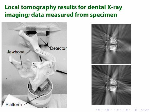
Applications to medical X-ray imaging
Outline
Continuous and discrete Bayesian inversion
The prototype problem: one-dimensional deconvolution
Total variation prior and the discretization dilemma
Wavelets and Besov spaces
Promoting sparsity using Besov space priors
Applications to medical X-ray imaging
Our starting point is the continuum modelfor an indirect measurement
Consider a quantity U that can be observed indirectly by
M = AU + E ,
where A is a smoothing linear operator, E is white noise,and U and M are functions.
In the Bayesian framework, U = U(x , ω), M = M(z , ω) andE = E(z , ω) are taken to be random functions.
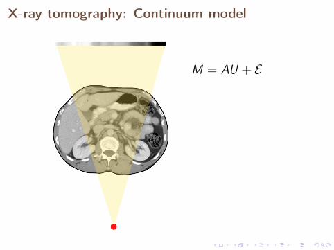
X-ray tomography: Continuum model
M = AU + E
A measurement device gives only a finite numberof data, leading to practical measurement model
The measurement is a realization of the random variable
Mk = PkM = AkU + Ek ,
where Ak = PkA and Ek = PkE . Here Pk is a linear orthogonalprojection with k-dimensional range.
The given data is a realization mk = Mk(z , ω0) of the measurementMk(z , ω), where ω0 ∈ Ω is a specific element in the probabilityspace.
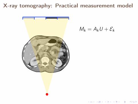
X-ray tomography: Practical measurement model
Mk = AkU + Ek
The inverse problem
This study concentrates on the inverse problem
given a realization mk , estimate U,
using estimates and confidence intervals related to a Bayesianposterior probability distribution.
Numerical solution of the inverse problem is basedon the discrete computational model
We need to discretize the unknown function U. Assume that U is apriori known to take values in a function space Y .
Choose a linear projection Tn : Y → Y with n-dimensional rangeYn, and define a random variable Un := TnU taking values in Yn.This leads to the computational model
Mkn = AkUn + Ek .
Note that realizations of Mkn can be simulated by computerbut cannot be measured in reality.
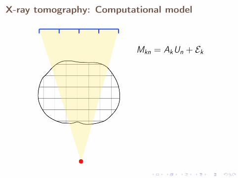
X-ray tomography: Computational model
Mkn = AkUn + Ek
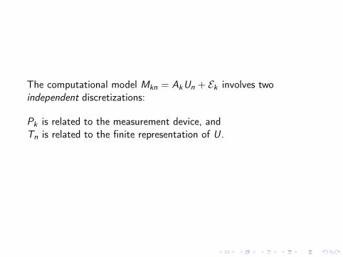
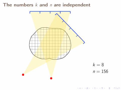
The computational model Mkn = AkUn + Ek involves twoindependent discretizations:
Pk is related to the measurement device, andTn is related to the finite representation of U.
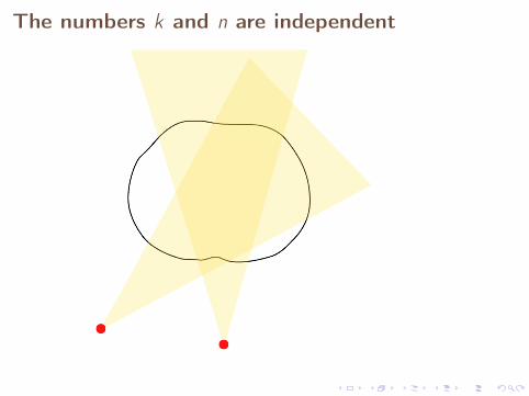
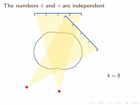
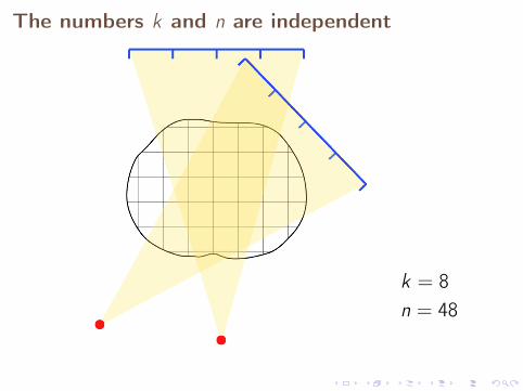
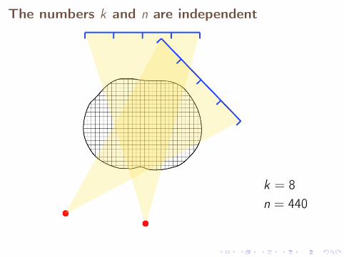
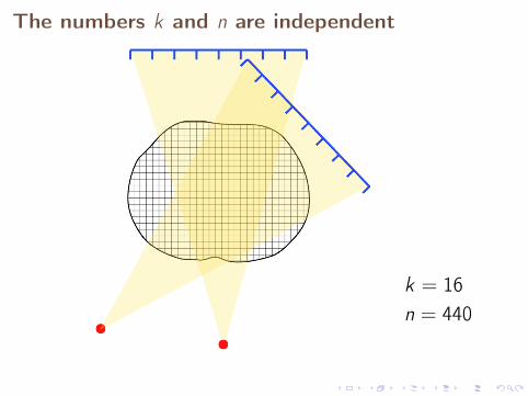
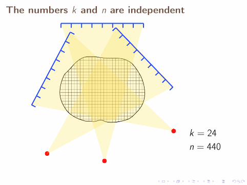
The numbers k and n are independent
The numbers k and n are independent
k = 8
The numbers k and n are independent
k = 8n = 48
The numbers k and n are independent
k = 8n = 156
The numbers k and n are independent
k = 8n = 440
The numbers k and n are independent
k = 16n = 440
The numbers k and n are independent
k = 24n = 440
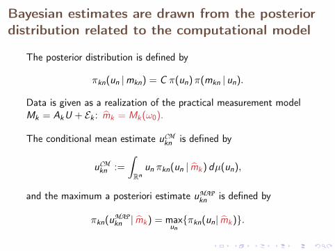
Bayesian estimates are drawn from the posteriordistribution related to the computational model
The posterior distribution is defined by
πkn(un |mkn) = C π(un)π(mkn | un).
Data is given as a realization of the practical measurement modelMk = AkU + Ek : mk = Mk(ω0).
The conditional mean estimate uCMkn is defined by
uCMkn :=
∫Rn
un πkn(un | mk) dµ(un),
and the maximum a posteriori estimate uMAPkn is defined by
πkn(uMAPkn | mk) = max
unπkn(un| mk).
We wish to construct discretization-invariantBayesian inversion strategies
We achieve discretization-invariance by constructing a well-definedinfinite-dimensional Bayesian framework, which can be projected toany finite dimension.
One advantage of discretization-invariance is that the priordistributions π(un) represent the same prior information at anydimension n. This is useful for delayed acceptance MCMCalgorithms, for example.
Discretization-invariant Bayesian estimatesbehave well as k →∞ and n→∞
Typically, a fixed measurement device is given, and k is constant.In that case, these limits should exist:
limn→∞
uCMkn and lim
n→∞uMAPkn .
On the other hand, we might have the opportunity to update ourdevice to a more accurate one, increasing k independently of n. Ifwe keep n fixed, the following limits should exist:
limk→∞
uCMkn and lim
k→∞uMAPkn .
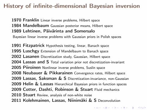
History of infinite-dimensional Bayesian inversion
1970 Franklin Linear inverse problems, Hilbert space1984 Mandelbaum Gaussian posterior means, Hilbert space1989 Lehtinen, Päivärinta and SomersaloBayesian linear inverse problems with Gaussian priors in Polish spaces
1991 Fitzpatrick Hypothesis testing, linear, Banach space1995 Luschgy Extension of Mandelbaum to Banach space2002 Lasanen Discretization study, Gaussian, Hilbert space2004 Lassas and S Total variation prior not discretization-invariant2005 Piiroinen Nonlinear inverse problems, Suslin space2008 Neubauer & Pikkarainen Convergence rates, Hilbert space2009 Lassas, Saksman & S Discretization-invariance, non-Gaussian2009 Helin & Lassas Hierarchical Bayesian priors in function spaces2009 Cotter, Dashti, Robinson & Stuart Fluid mechanics2010 Stuart Review, analysis of non-white noise2011 Kolehmainen, Lassas, Niinimäki & S Deconvolution
Outline
Continuous and discrete Bayesian inversion
The prototype problem: one-dimensional deconvolution
Total variation prior and the discretization dilemma
Wavelets and Besov spaces
Promoting sparsity using Besov space priors
Applications to medical X-ray imaging
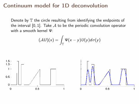
Continuum model for 1D deconvolution
n = 64
Denote by T the circle resulting from identifying the endpoints ofthe interval [0, 1]. Take A to be the periodic convolution operatorwith a smooth kernel Ψ:
(AU)(x) =
∫T
Ψ(x − y)U(y)dσ(y)
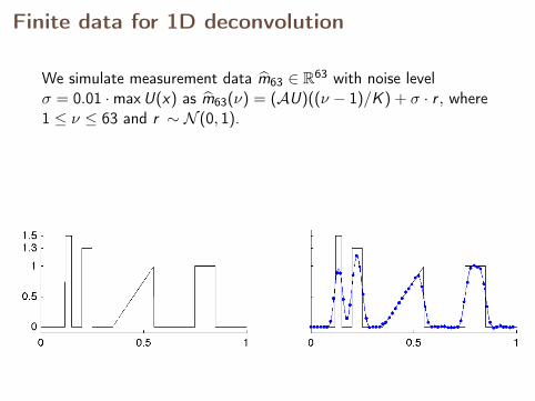
Finite data for 1D deconvolution
n = 64
We simulate measurement data m63 ∈ R63 with noise levelσ = 0.01 ·maxU(x) as m63(ν) = (AU)((ν − 1)/K ) + σ · r , where1 ≤ ν ≤ 63 and r ∼ N (0, 1).
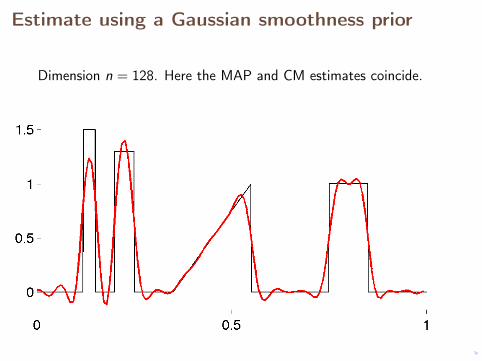
Estimate using a Gaussian smoothness prior
Dimension n = 128. Here the MAP and CM estimates coincide.
Outline
Continuous and discrete Bayesian inversion
The prototype problem: one-dimensional deconvolution
Total variation prior and the discretization dilemma
Wavelets and Besov spaces
Promoting sparsity using Besov space priors
Applications to medical X-ray imaging
Bayesian inversion using total variation prior
Theorem (Lassas and S 2004)Total variation prior is not discretization-invariant.
Sketch of proof: Apply a variant of the central limit theorem tothe independent, identically distributed random consecutivedifferences.
New numerical experiments are reported inKolehmainen, Lassas, Niinimäki and S (submitted).
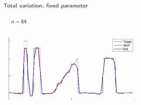
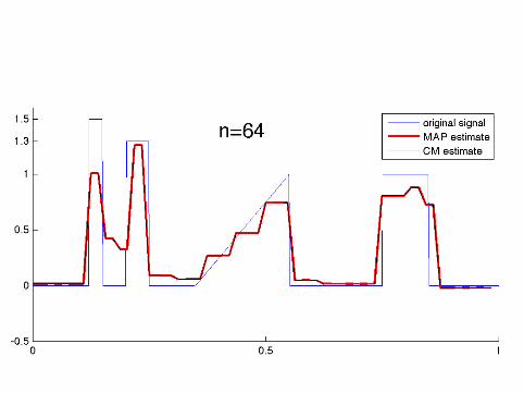
Total variation, fixed parameter
n = 64
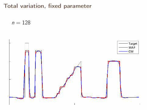
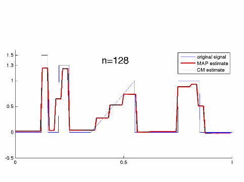
Total variation, fixed parameter
n = 128
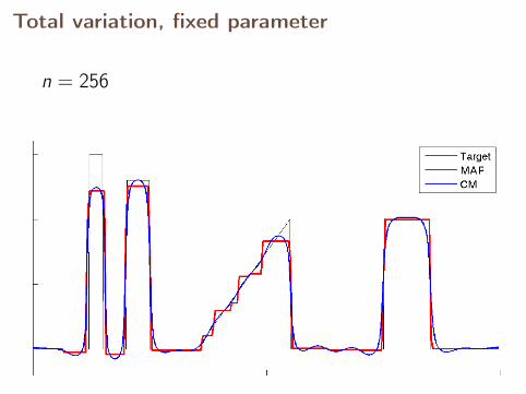
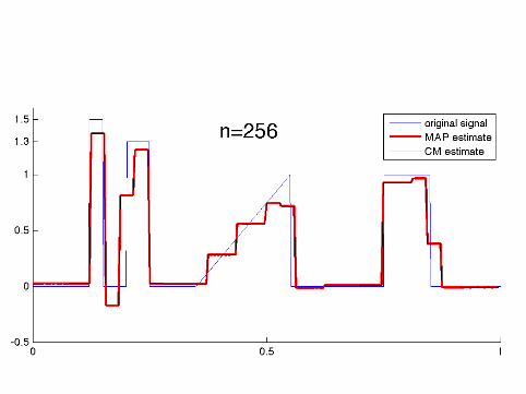
Total variation, fixed parameter
n = 256
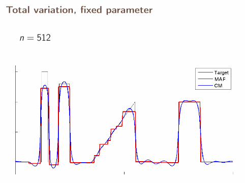
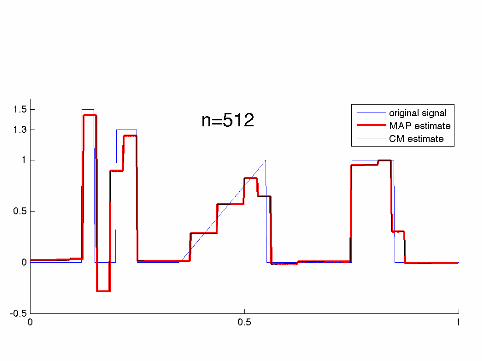
Total variation, fixed parameter
n = 512
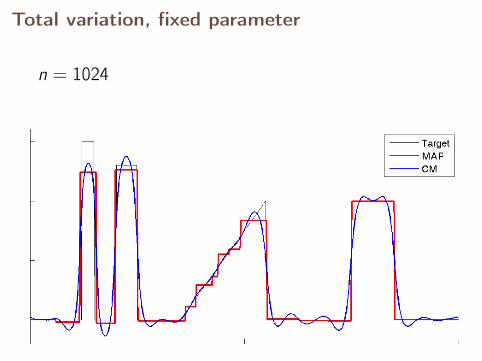
Total variation, fixed parameter
n = 1024
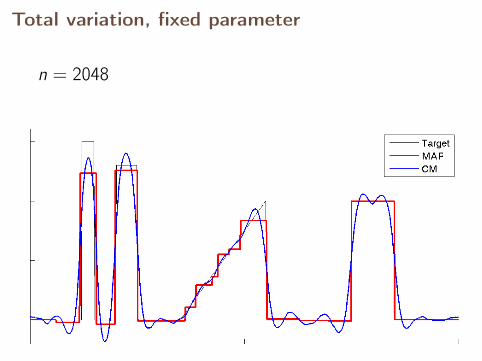
Total variation, fixed parameter
n = 2048
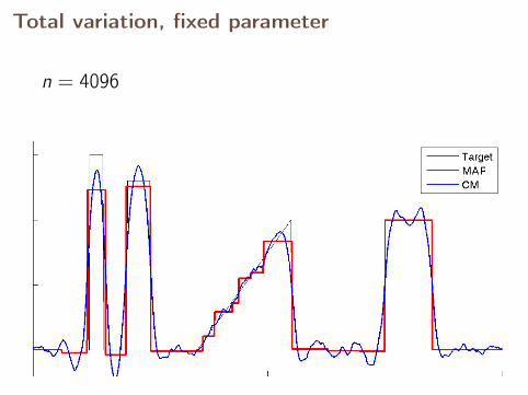
Total variation, fixed parameter
n = 4096
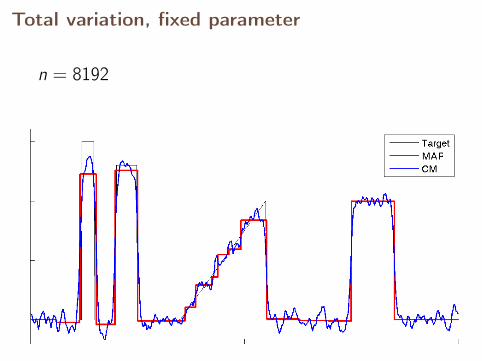
Total variation, fixed parameter
n = 8192
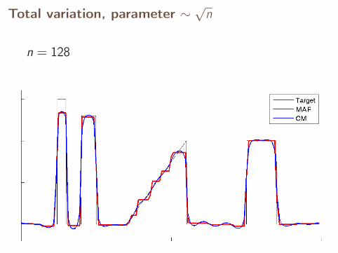
With fixed parameter, the MAP estimates converge,but CM estimates diverge.
Let’s see what happens with a parameter scaled as√
n.
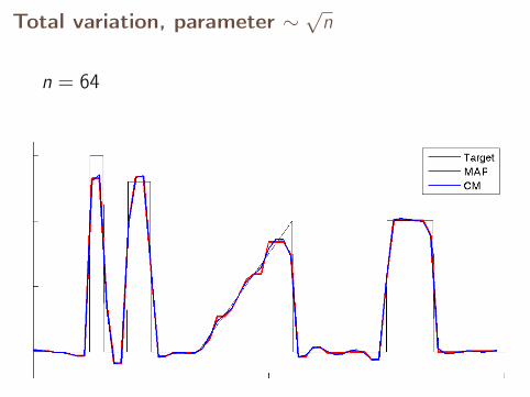
Total variation, parameter ∼√
n
n = 64
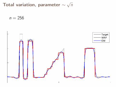
Total variation, parameter ∼√
n
n = 128
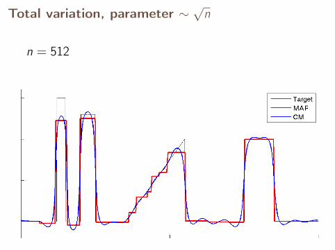
Total variation, parameter ∼√
n
n = 256
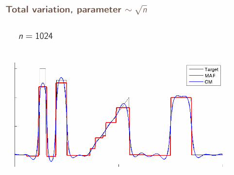
Total variation, parameter ∼√
n
n = 512
Total variation, parameter ∼√
n
n = 1024
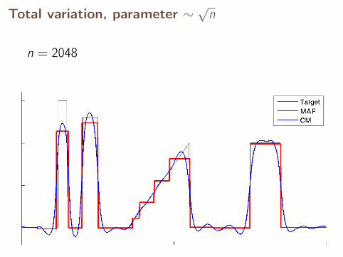
Total variation, parameter ∼√
n
n = 2048
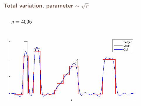
Total variation, parameter ∼√
n
n = 4096
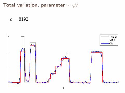
Total variation, parameter ∼√
n
n = 8192

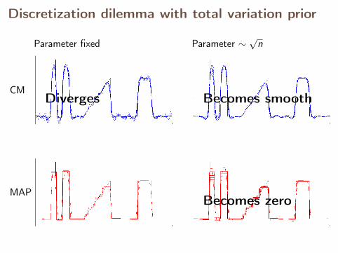
Discretization dilemma with total variation prior
CM
MAP
Parameter fixed Parameter ∼√
n
Discretization dilemma with total variation prior
CM
MAP
Parameter fixed Parameter ∼√
n
Diverges Becomes smooth
Becomes zero
Outline
Continuous and discrete Bayesian inversion
The prototype problem: one-dimensional deconvolution
Total variation prior and the discretization dilemma
Wavelets and Besov spaces
Promoting sparsity using Besov space priors
Applications to medical X-ray imaging
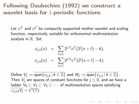
Following Daubechies (1992) we construct awavelet basis for 1-periodic functions
Let ψC and φC be compactly supported mother wavelet and scalingfunction, respectively, suitable for orthonormal multiresolutionanalysis in R. Set
φj ,k(x) =∑`∈Z
2j/2φC (2j(x + `)− k),
ψj ,k(x) =∑`∈Z
2j/2ψC (2j(x + `)− k).
Define Vj := spanφj ,k | k ∈ Z and Wj := spanψj ,k | k ∈ Z.Then Vj are spaces of constant functions for j ≤ 0, and we have aladder V0 ⊂ V1 ⊂ V2 ⊂ · · · of multiresolution spaces satisfying∪j≥0Vj = L2(T).
Wavelet decomposition divides a function intodetails at different scales
We can write
U(x) = c0 +∞∑j=0
2j−1∑k=0
wj ,k ψj ,k(x),
where c0 = 〈U, φ0,0〉 and wj ,k = 〈U, ψj ,k〉.
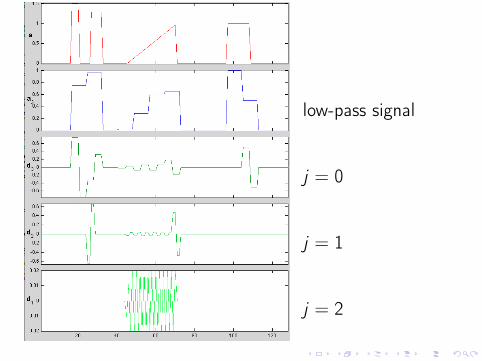
low-pass signal
j = 0
j = 1
j = 2
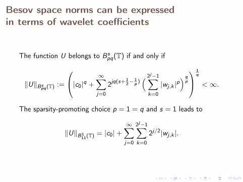
Besov space norms can be expressedin terms of wavelet coefficients
The function U belongs to Bspq(T) if and only if
‖U‖Bspq(T) :=
|c0|q +∞∑j=0
2jq(s+ 12−
1p )( 2j−1∑
k=0
|wj ,k |p) q
p
1q
<∞.
The sparsity-promoting choice p = 1 = q and s = 1 leads to
‖U‖B111(T)
= |c0|+∞∑j=0
2j−1∑k=0
2j/2|wj ,k |.
Outline
Continuous and discrete Bayesian inversion
The prototype problem: one-dimensional deconvolution
Total variation prior and the discretization dilemma
Wavelets and Besov spaces
Promoting sparsity using Besov space priors
Applications to medical X-ray imaging
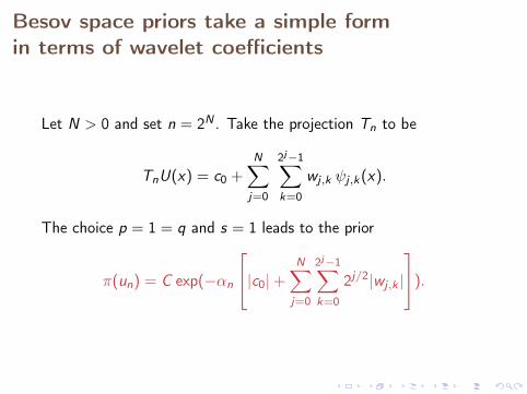
Besov space priors take a simple formin terms of wavelet coefficients
Let N > 0 and set n = 2N . Take the projection Tn to be
TnU(x) = c0 +N∑
j=0
2j−1∑k=0
wj ,k ψj ,k(x).
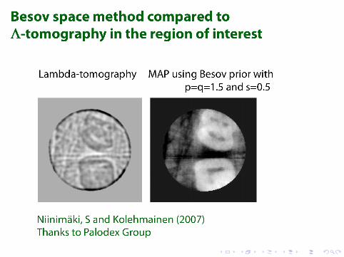
The choice p = 1 = q and s = 1 leads to the prior
π(un) = C exp(−αn
|c0|+N∑
j=0
2j−1∑k=0
2j/2|wj ,k |
).
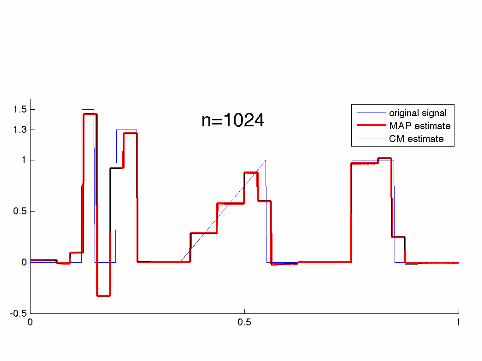
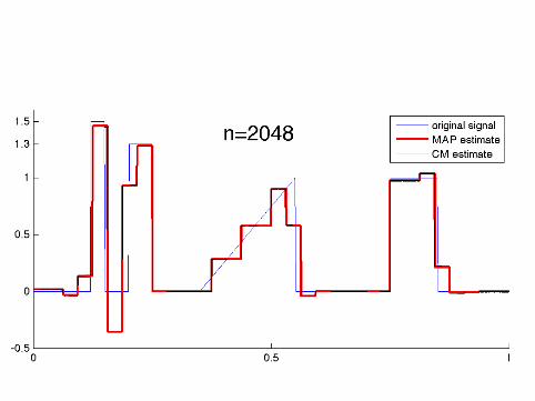
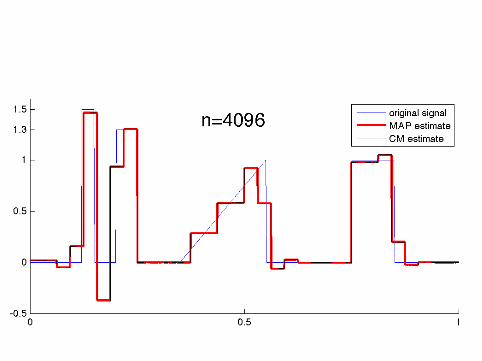
Bayesian inversion using Besov space priors
Theorem (Lassas, Saksman and S 2009)Besov space priors are discretization-invariant.
Sketch of proof: Construction of well-defined Bayesian inversiontheory in infinite-dimensional Besov spaces that allow wavelet bases.Discretizations are achieved by truncating the wavelet expansion.
Numerical experiments are reported inKolehmainen, Lassas, Niinimäki and S (submitted).
Deterministic Besov space regularization was first introduced inDaubechies, Defrise and De Mol 2004.
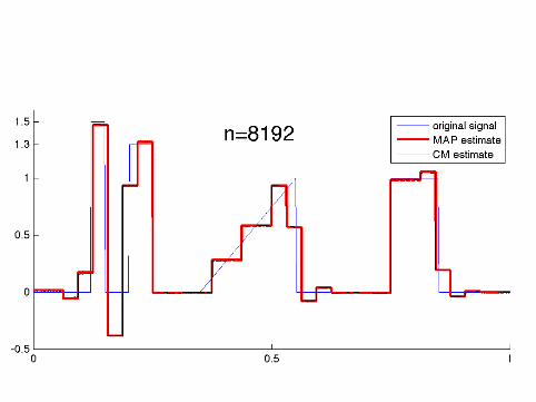
Computational implementation required specialalgorithms as the dimension went up to n = 8192
The MAP estimates were computed using a tailored QuadraticProgramming algorithm.
The CM estimates were computed using the Metropolis-Hastingsalgorithm and a random one-element scanning scheme.
Details of the implementation can be found inKolehmainen, Lassas, Niinimäki and S (submitted).
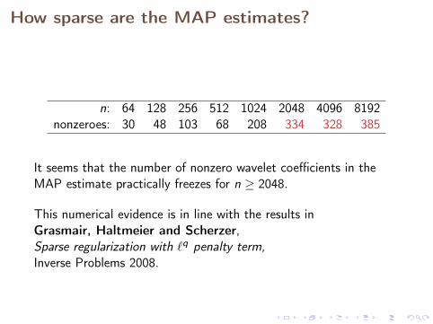
How sparse are the MAP estimates?
n: 64 128 256 512 1024 2048 4096 8192nonzeroes: 30 48 103 68 208 334 328 385
It seems that the number of nonzero wavelet coefficients in theMAP estimate practically freezes for n ≥ 2048.
This numerical evidence is in line with the results inGrasmair, Haltmeier and Scherzer,Sparse regularization with `q penalty term,Inverse Problems 2008.
Outline
Continuous and discrete Bayesian inversion
The prototype problem: one-dimensional deconvolution
Total variation prior and the discretization dilemma
Wavelets and Besov spaces
Promoting sparsity using Besov space priors
Applications to medical X-ray imaging
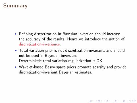
Summary
I Refining discretization in Bayesian inversion should increasethe accuracy of the results. Hence we introduce the notion ofdiscretization-invariance.
I Total variation prior is not discretization-invariant, and shouldnot be used in Bayesian inversion.Deterministic total variation regularization is OK.
I Wavelet-based Besov space priors promote sparsity and providediscretization-invariant Bayesian estimates.

Thank you for your attention!
Preprints available at www.siltanen-research.net.