HAL Id: hal-01328559https://hal.inria.fr/hal-01328559

Submitted on 8 Jun 2016

HAL is a multi-disciplinary open accessarchive for the deposit and dissemination of sci-entific research documents, whether they are pub-lished or not. The documents may come fromteaching and research institutions in France orabroad, or from public or private research centers.

L’archive ouverte pluridisciplinaire HAL, estdestinée au dépôt et à la diffusion de documentsscientifiques de niveau recherche, publiés ou non,émanant des établissements d’enseignement et derecherche français ou étrangers, des laboratoirespublics ou privés.

Distributed under a Creative Commons Attribution| 4.0 International License

SPARK – A Bushfire Spread Prediction ToolClaire Miller, James Hilton, Andrew Sullivan, Mahesh Prakash

To cite this version:Claire Miller, James Hilton, Andrew Sullivan, Mahesh Prakash. SPARK – A Bushfire Spread Pre-diction Tool. 11th International Symposium on Environmental Software Systems (ISESS), Mar 2015,Melbourne, Australia. pp.262-271, �10.1007/978-3-319-15994-2_26�. �hal-01328559�

SPARK - a Bushfire Spread Prediction Tool

Claire Miller1, James Hilton1, Andrew Sullivan2, and Mahesh Prakash1

1CSIRO Digital Productivity Flagship, Melbourne, Australia {claire.miller, james.hilton, mahesh.prakash}@csiro.au

2CSIRO Land and Water Flagship, Canberra, Australia andrew.sullivan@csiro.au

Abstract. Bushfires are complex processes, making it difficult to accurately predict their rate of spread. We present an integrated software system for bush-fire spread prediction, SPARK, which was developed with the functionality to model some of these complexities. SPARK uses a level set method governed by a user-defined algebraic spread rate to model fire propagation. The model is run within a modular workflow-based software environment. Implementation of SPARK is demonstrated for two cases: a small-scale experimental fire and a complex bushfire scenario. In the second case, the complexity of environmental non-homogeneity is explored through the inclusion of local variation in fuel and wind. Simulations over multiple runs with this fuel and wind variation are ag-gregated to produce a probability map of fire spread over a given time period. The model output has potential to be used operationally for real-time fire spread modeling, or by decision makers predicting risk from bushfire events. Keywords: level set, bushfire, wildfire, modeling, simulation

1 Introduction

Although a natural occurrence in the Australian landscape, bushfires have the ability to be devastating, particularly when they come into contact with urban environments. Improving knowledge of how these fires spread is critical for effective management and timely issuing of warnings. Unfortunately, it is difficult to predict the rate of spread of a fire as there are many elements influencing fire behavior occurring over a range of length and time scales. Fully physical computational fluid dynamics models attempt to incorporate a large number of these elements, but are computationally in-tensive and are not practical in an operational environment. Instead, operational mod-els usually propagate the perimeter of the fire using spread rates based on empirical expressions. These empirical models can give an approximation of expected fire area in a significantly shorter computational time than physical models.

Two operational tools currently in use in Australia are Phoenix Rapidfire [1] and Australis [2], both developed over the last ten years. SPARK has been developed with the goal of easy adaptability. It allows user defined spread models, as opposed to the

adfa, p. 1, 2011. © Springer-Verlag Berlin Heidelberg 2011

hard-coded spread models found in current operational tools. This functionality ena-bles many aspects of simulated fire spread to be tested and investigated. One such aspect is the non-homogeneity of a bushfire’s local environment, which we explore in this paper.

This paper aims to familiarize readers with SPARK’s architecture and development path, and to demonstrate its analysis capability for a simple fire scenario. We explore the functionality of SPARK in dealing with non-homogeneity, which highlights the requirement for correct consideration of local environmental conditions.

2 SPARK Overview

SPARK uses a level set method for the representation of the fire perimeter, which propagates over a domain according to a one-dimensional algebraic rate of spread. The model sits within a workflow environment, allowing a broad range of flexibility in the analysis and the input and output of data types. Core elements of the model are explained in further detail below, along with details on the data aspects of the tool.

2.1 Level Set Method

The level set method is used to model the propagation of the fire perimeter. Use of this method is still fairly novel for fire simulation, particularly for large-scale wildland fires. The level set method was first implemented as an interface propagation solution by [3] and has since been found useful over multiple application areas (eg. [4] and [5]). In contrast to traditional simulation methods which define front locations and propagate these locations forward in time, the level set method defines a surface over the domain according to a distance function. In this implementation the value of the distance function, Φ, is equal to the closest distance to the fire perimeter. The function is defined as positive where the fire is yet to burn and negative in burnt areas. This allows for simple identification of the front location at Φ = 0. Evolution of the surface in time is determined for each grid cell using some rate of spread value, S, in a direction normal to the fire front, according to

𝜕𝜕Φ𝜕𝜕𝜕𝜕

+ 𝑆𝑆|∇Φ| = 0. (1)

For a more detailed explanation of the model, see [6].

2.2 One Dimensional Spread Rates

The value of S in Equation (1) is calculated for each cell according to a one dimen-sional rate of spread model. This spread rate model is a function of the environmental conditions at that grid point. The level set method in SPARK uses OpenCL [7], allow-ing the spread rate model governing the value of S to be directly passed to the OpenCL compiler as a text string written in the C programming language. This allows

the flexibility of incorporating a range of aspects and functional forms of fire spread model. An example input is shown in the lower right panel of Fig. 1.

2.3 Workflow System

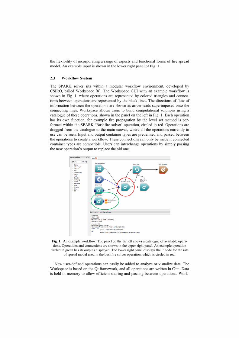
The SPARK solver sits within a modular workflow environment, developed by CSIRO, called Workspace [8]. The Workspace GUI with an example workflow is shown in Fig. 1, where operations are represented by colored triangles and connec-tions between operations are represented by the black lines. The directions of flow of information between the operations are shown as arrowheads superimposed onto the connecting lines. Workspace allows users to build computational solutions using a catalogue of these operations, shown in the panel on the left in Fig. 1. Each operation has its own function, for example fire propagation by the level set method is per-formed within the SPARK ‘Bushfire solver’ operation, circled in red. Operations are dragged from the catalogue to the main canvas, where all the operations currently in use can be seen. Input and output container types are predefined and passed between the operations to create a workflow. These connections can only be made if connected container types are compatible. Users can interchange operations by simply passing the new operation’s output to replace the old one.

Fig. 1. An example workflow. The panel on the far left shows a catalogue of available opera-tions. Operations and connections are shown in the upper right panel. An example operation

circled in green has its outputs displayed. The lower right panel displays the C code for the rate of spread model used in the bushfire solver operation, which is circled in red.

New user-defined operations can easily be added to analyze or visualize data. The Workspace is based on the Qt framework, and all operations are written in C++. Data is held in memory to allow efficient sharing and passing between operations. Work-

space allows the data to be read and written at any stage of workflow operation. This allows users to visualize progressive fire spread output from SPARK. New operations and data types are compiled as shared libraries (.dll, .so or .dylib) which act as plugins to Workspace. For example, the SPARK model and analysis operations are all con-tained within a single plugin. This plugin architecture allows transparent access be-tween different data types and operations within the framework. C++ stub code for new operations and data types can be generated using code generation wizards and compiled using the included CMake build system and scripts for cross platform com-pilation.

As well as the Workspace GUI shown in Fig. 1, workflow execution is supported from the command line through batch execution or exposed through an API. Close integration with Qt allows complex user interfaces to be designed and transparently connected with an underlying workflow, allowing custom applications to be easily developed. Parallel APIs, such as OpenMP and OpenCL, are fully supported. Opera-tions for running scripts in both ECMAScript and Python within Workspace are also available for non C++ developers. Furthermore, a number of existing open-source software systems have been natively compiled with the Workspace framework. These modules include; OpenCV for image analysis, which can be used to convert fire im-agery to SPARK inputs, NetCDF for large data file support, which is useful for SPARK’s environmental inputs and spread information outputs, and GDAL for geo-spatial analysis and conversion, which can convert to meter grids from latitudes and longitudes for compatibility with fire spread rate equations.

2.4 Integration with the Amicus Decision Support Tool

SPARK has been built with the capability to be integrated with the decision support tool Amicus [9] through Workspace. Amicus is a knowledge base and tool informing users on expected fire behavior metrics given a set of fuel, weather, and topographic conditions. It has been built around a number of well-established fire spread models developed for Australian vegetation. The rate of spread model functions in Amicus exist as separate operations within Workspace and can be used and tested within Amicus before being implemented dynamically within SPARK.

2.5 Data Inputs

Fires can occur over a vast range of vegetation and fuel types. By using gridded in-puts for fuel properties it is possible for a variety of fuel types to occur within the same simulation, bounded only by grid size. This can include areas of un-burnable fuel, such as roads and water bodies. The development of SPARK within a workflow environment allows users to easily incorporate these environmental inputs. Fuel grids can be pre-populated and read directly into the workflow, or manipulated from other inputs, such as satellite imagery, within the workflow.

Weather conditions, in particular significant changes in weather conditions, con-tribute significantly to fire consequence. Atmospheric condition inputs, which often include air temperature, relative humidity, wind speed, and wind direction, are gener-

ated as time series. The time series inputs for the model are implemented as a Work-space data type with arbitrary temporal spacing between the samples.

2.6 Data Sources

In order to run SPARK, data is required for the atmospheric conditions, fuel condi-tions, topography, and initial fire location. This can be sourced from a range of data-bases discussed below, depending on the scenario. A current aim is to integrate web services into the model, such that data can be directly used by the system.

Historical data for atmospheric conditions are available from the Australian Bureau of Meteorology at half hourly intervals for a number of stations nationally. This data can be used to set parameters such as the wind, temperature, and moisture levels for simulating large historical fire events. Issues arise when the stations available are not close, in both location and environment, to the ignition location. In the future, we hope to gain access to data recorded during fire events, or gridded hindcast data, which may provide a more accurate record of the conditions. For small experimental fires, such as the case demonstrated in Section 3, atmospheric data is commonly rec-orded at a high frequency in locations close to the fire.

Fuel inputs are slightly more difficult to obtain. They can be manually created us-ing basic satellite imagery, such as from Google maps. A related, but more sophisti-cated, method is to create classifications using satellite band imagery from LandSat. A third option is to use land use grids which can be converted to fuel types, however these tend to lack the critical details of unburnable areas such as roads and water bod-ies. Which of these inputs are most useful depends on the scale of the area of interest and the fuel information that is required for the rate of spread formula used.

The last input is initial fire location information. Fire ignition locations and pro-gression maps are available online for some historical fires and hence are simple to implement. For more recent fires, fire agencies will often use airborne thermal image-ry to determine current fire extent. This imagery is geo-tagged and can be converted to a fire front map. For example, some images may be false colored with the fire ap-pearing as red in the image with the surrounding area blue. It is straightforward to split the image by color and threshold according to the value of the red channel. Addi-tionally, this entire process can be performed within the workflow.

2.7 Data Output

The output from SPARK consists of gridded forms of both the value of the level set function at a user specified frequency and the time of ignition over the domain. This allows users to easily investigate both long term and time specific consequence of the fire.

3 A Simple Fire Scenario

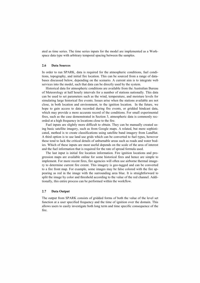
A series of small scale, 35 m square, experimental burns were conducted in Ballarat, Victoria, Australia in January, 2014 [10]. Weather data was recorded during the fires, for both the wind speed and bearing, at a frequency of 10 Hz. The fire used in this example burnt for 28 seconds, with wind speeds averaging around 4 ms-1. Quad-copter footage was taken of each fire, which was then stabilized and rectified to pro-vide clear observations of the spread.

Fig. 2. A simple fire example. Simulated fire fronts (solid white line) are overlaid on fire im-

agery for the ignition configuration, left, and then at 25 seconds, right.

For this example, simulated spread was governed by a generic rate of spread model with an added curvature dependent component. The grid size was 0.1 m. A qualitative comparison of simulated spread to actual fire imagery indicates a good match for both fire shape and rate of spread, as shown in Fig. 2. This is largely influenced by the ability to incorporate curvature. Without the inclusion of a shape-related variable in the spread model, simulated fires on flat ground tend to maintain their initial shape.

4 A Study of Non-Homogeneity

A major challenge in simulating bushfire spread is dealing with the complexities of the environments in which they occur. This can include complex topographies, often large varieties of fuel types, and local variations in weather and fuel. Operational fire spread models developed for large scale fires assume fires will attain a quasi-steady rate of spread for conditions averaged over considerable time and distance, invariably smoothing out local scale environmental variations. SPARK was used to investigate the effect of this local variation on fire spread. The use of a gridded input system al-lows the methods for the inclusion of variation explained below to be simply imple-mented. The application of these mechanisms is demonstrated in Section 5.

4.1 The Inclusion of Variation

At most scales, our environment is far from homogeneous. The software architecture has the functionality to easily incorporate spatial and temporal variation into both the fuel and wind inputs.

In order to include fuel variation, a grid was populated prior to the running of the model. Fuel values for each cell were chosen randomly, and independently of sur-rounding cells, from a predefined distribution. The distribution used could be different for different fuel varieties according to a fuel input grid. The random selection pro-cess enabled reproducibility by setting a seed value for the random number generator. Fig. 3 is a diagram showing the fuel population process.

Fig. 3. The process by which fuel grids are populated. The left column focuses on the definition of multiple fuel types, the right column focuses on the incorporation of variation into the grid.

Variation was also included in wind, for both speed and direction, in a similar manner. For the wind however, the value of each parameter was randomly chosen from its predefined distribution for each grid cell spread calculation at each time step. For this preliminary investigation, the variation in both fuel and wind was assumed to be normally distributed.

The workflow system allowed the implementation of variation to be straightfor-wardly incorporated in the execution of the model. The seed value was given to a random number generation operation which gave a new random value every time one was requested. The random operation in this case was used for both the population of the fuel layer and the wind strength and direction.

4.2 Probability of Arrival Maps

The addition of variation into the model in this manner adds an element of random-ness into the arrival time of the fire at a given location. As such, the same simulation run with a different randomly selected set of environmental values, based on the same distributions, could potentially produce a different set of arrival times. This leads to the concept of an ensemble of simulations run with different seed values for the ran-dom selection process. Producing intuitive visualizations of these results is challeng-ing. The method we use in this paper is maps indicating the probability of arrival of the fire. These maps show, for each grid cell, the proportion of simulations in which the front passed through that cell in a given time frame. As such, they can give an indication of the probability of the fire reaching a location at a given time.

5 Complex Fire Scenario with Variation

The Deans Gap fire burned within the City of Shoalhaven, New South Wales, Aus-tralia, for over a week in January, 2013 [11]. It was a highly complex fire in terms of weather, fuel, and topography. Consequently, it provides an interesting scenario in which to demonstrate how the addition of variation can provide an increased under-standing of expected spread. Our scenario focused on the first 24 hours, January 7th to 8th. Fire location data was obtained from the NSW Rural Fire Service.

For these simulations the Dry Eucalypt Fire Model [12] rate of spread for Australi-an forest vegetation was used. This rate of spread model was chosen as it is the most suitable for the vegetation in the fire area. The domain was an 850 by 740 grid with a cell size of just less than 30 m. Total simulated fire time was 31 hours. Wind was a triangulation of data from the surrounding weather stations of Nowra, Ulladulla, Jer-vis Bay, and Goulburn. The variation in the wind had standard deviation 1 km/h and 10 degrees for speed and direction respectively. Fuel height was variable with mean 50 cm and standard deviation 30 cm. The surface fuel hazard score used in the model was 2, and near-surface fuel hazard 3.5. Maximum slope over which the fire was con-sidered able to run was 40 degrees.

Simulation results for several times are shown in Fig. 4a. Results indicate a slow spread over the first 12 hours, which is the period over the evening and night. The fire picks up during the morning of the next day as the temperature starts to heat up. There is a further increase in spread rate in the afternoon, which is the hottest and driest time of day, as would be expected.

The concept of a probability of arrival map was applied to the Deans Gap scenario using 100 simulations run from different seeds, Fig. 4b. This map highlights that the

addition of variation over a 24 hour period, from a known ignition location, has a significant impact on spread. Within the 10 minute interval possible front locations stretch almost four and a half kilometers. These results show how unpredictable the fire can be, and in which areas this variation is greatest. This has implications both educationally and operationally. It shows that the influence of common local envi-ronmental events can have an impact on the final spread, which the straight empirical models do not capture. Operationally, it provides an enhanced knowledge set to assist decision making.

(a) (b)

Fig. 4. Simulation results for Deans Gap; (a) A single simulation with the ignition point (yel-low, top left) at 17:30 on January 7, and the simulation results for each subsequent 6 hourly

interval finishing at 17:30 on January 8. Each new 6 hour interval is represented by a change in color, (b) Probability of arrival map for the time frame 17:20 to 17:30 on January 8. Red indi-cates a high proportion, and blue low, of simulations predicting the same arrival time in each

cell.

6 Summary

We have provided a general introduction to SPARK, our bushfire prediction tool. The model uses a level set method for fast and simple spread propagation, combined with well-established empirical spread rates. The simple fire example demonstrated the use of a generic fire spread rate that incorporated curvature.

SPARK has been developed with the goal of providing the functionality to easily incorporate, and hence investigate, additional complexities in the model. The use of a visual workflow tool such as Workspace has made this relatively straightforward to do. This is expected to be useful for researchers to determine the roles and importance of these complexities. The complexity considered here was the addition of variation into the environmental components. Applying this to a complex bushfire scenario has indicated that this variation over an extended period of time can introduce a large amount of uncertainty into the results. Highlighting this effect, and the areas in which it is most significant, could potentially provide a more well-informed information set to fire management.

SPARK is currently being used to further investigate the effect of this variation. Future work will also be to consider the inclusion of wind and spotting models.

References

1. Tolhurst, K., Shields, B., Chong, D., 2008. Phoenix: development and application of a bushfire risk management tool. The Australian Journal of Emergency Management 23, 47-54.

2. Johnston, P., Kelso, J., Milne, G. J., 2008. Efficient simulation of wildfire spread on an ir-regular grid. International Journal of Wildland Fire 17, 614–627.

3. Osher, S, Sethian, J., 1988. Fronts Propagating with Curvature-Dependent Speed: Algo-rithms Based on Hamilton-Jacobi Formulations. Journal of Computational Physics 79 (1), 12-49.

4. Sethian, J.A., Strain, J., 1992. Crystal growth and dendritic solidification. Journal of Com-putational Physics 98 (2), 231-253.

5. Sussman, M., Smereka, P., Osher, S., 1994. A level set approach for computing solutions to incompressible two-phase flow. Journal of Computational Physics 114, 146-159.

6. Hilton, J., Miller, C., Sullivan, A., Rucinski, C., Under Review. Incorporation of variation into wildfire spread models using a level set approach. Submitted to Environmental Mod-elling and Software.

7. OpenCL, 2014. https://www.khronos.org/opencl/. Accessed 9 December, 2014. 8. Workspace, 2014. http://research.csiro.au/workspace/. Accessed 31 October, 2014. 9. Sullivan, A.L., Gould, J.S., Cruz, M.G., Rucinski,C., Prakash, M., 2013. Amicus: a nation-

al fire behaviour knowledge base for enhanced information management and better deci-sion making. In: Piantadosi, J.; Anderssen, R. S. & J., B. (Eds.) MODSIM2013, 20th In-ternational Congress on Modelling and Simulation, pp. 2068-2074.

10. Cruz, M.G., Gould, J., Kidnie, S., Nichols, D., Anderson, W.R., Bessel, R., Hurley, R., Koul, V., Under Review. Grass curing and fire behavior. Submitted to International Jour-nal of Wildland Fire.

11. Mackie, B, McLennan, J, Wright, L. 2013. Community Understanding and Awareness of Bushfire Safety: January 2013 Bushfires. Research for the New South Wales Rural Fire Service. Bushfire CRC. La Trobe University.

12. Cheney, N.P., Gould, J.S., McCaw, W.L., Anderson, W.R., 2012. Predicting fire behaviour in dry eucalypt forest in southern Australia. Forest Ecology and Management 280, 120-131.