Spanish-inﬂuenced prosody in Miami...

Spanish-influenced prosody in Miami English

Naomi Enzinna∗

1 Introduction

In 2013, various news organizations—including the Miami Herald, Sun Sentinel, andBusiness Insider—published articles on the emergence of an English dialect unique to Mi-ami. Due to frequent and prolonged contact between Spanish and English in South Florida,this Miami English dialect is claimed to have the following characteristics: subtle vowelshading, a palatalized L,1 and a “syllable-timed” rhythm. Additionally, Miami English issaid to include Spanish-inspired calques. “For example, instead of saying, ‘let’s get out ofthe car,’ someone from Miami might say, ‘let’s get down from the car’ because of the Span-ish phrase bajar del coche” (Watts, 2013). According to sociolinguist Phillip M. Carter,Miami English is spoken by Miami natives: “What’s noteworthy about Miami English isthat we’re now in a third, even fourth generation of kids who are using these features ofnative dialect. So we’re not talking—and let me be clear—we’re not talking about non-native features. These are native speakers of English who have learned a variety influencedhistorically by Spanish” (Haggin, 2013). However, little systematic study has been doneyet to support these impressionistic observations.

This study aims to test these claims using linguistically sound measures, taking intoaccount various influencing factors and narrowing in on a single property of the dialect:prosody. More specifically, this study investigates the influence of Miami’s high Hispanicpopulation on the variety of English spoken in Miami. In 2013, 65.6% of Miami-DadeCounty was Hispanic (U.S. Census Bureau, 2014). However, this percentage varied widelyacross the county. For example, Hialeah’s population was 94.7% Hispanic, while Aven-tura’s population was only 35.8% Hispanic (U.S. Census Bureau, 2014). Considering thesedifferences, this study aims to address whether neighborhood demographics influence whoacquires this Spanish-influenced English variety. Additionally, this study investigates theinfluence of parent language and L2 age of acquisition.

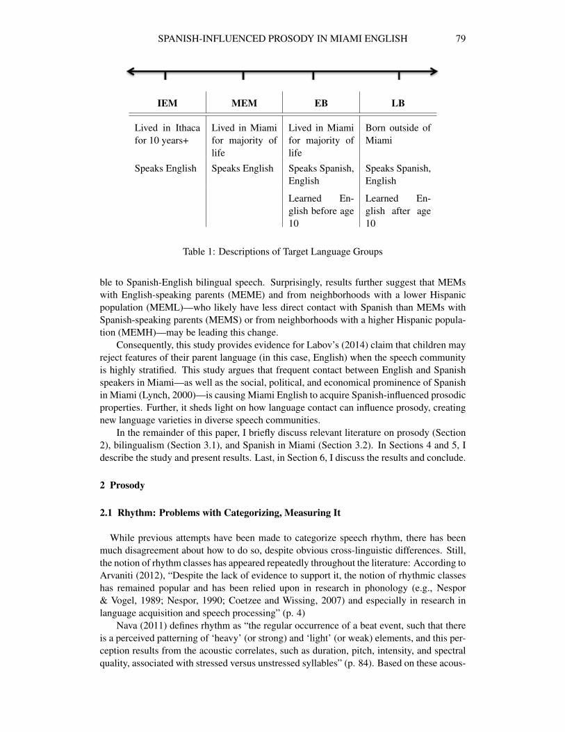
The language groups investigated in this study are (1) English monolinguals from Mi-ami,2 (2) English monolinguals from Ithaca,3 (3) Spanish-English bilinguals who are fromMiami and learned English at an early age, and (4) Spanish-English bilinguals who are notfrom Miami and learned English at a later age—henceforth, MEMs (Miami English Mono-linguals), IEMs (Ithaca English Monolinguals), EBs (Early Spanish-English Bilinguals),and LBs (Late Spanish-English Bilinguals), respectively. Basic descriptions of these par-ticipant groups are presented in Table 1. The continuum (arrow) represents each group’spredicted similarity to English (left) and/or Spanish (right).

To compare the prosody of these language groups, read speech was collected andcompared using rhythm (Ramus et al., 1999) and pitch (Kelm, 1995) metrics. Resultsshow that MEMs’ rhythm and pitch differ from (non-Miami) English and are compara-

∗I thank Sam Tilsen for guidance and feedback, as well as Abby Cohn; Draga Zec; Phillip M. Carter; andthe members of the Cornell Phonetics Lab, Phonetics Data Analysis Working Group, and Research Workshop.

1This is called a heavy L in the article.2Monolingual participants may have studied a second language in high school or university; however, they

do not feel confident in their ability to speak a second language.3This group is meant to be representative of English monolinguals with speech not influenced by Spanish.

Ithaca’s Hispanic population in 2013 was 6.9% (U.S. Census Bureau, 2014).

SPANISH-INFLUENCED PROSODY IN MIAMI ENGLISH 79

IEM MEM EB LB

Lived in Ithacafor 10 years+

Lived in Miamifor majority oflife

Lived in Miamifor majority oflife

Born outside ofMiami

Speaks English Speaks English Speaks Spanish,English

Speaks Spanish,English

Learned En-glish before age10

Learned En-glish after age10

Table 1: Descriptions of Target Language Groups

ble to Spanish-English bilingual speech. Surprisingly, results further suggest that MEMswith English-speaking parents (MEME) and from neighborhoods with a lower Hispanicpopulation (MEML)—who likely have less direct contact with Spanish than MEMs withSpanish-speaking parents (MEMS) or from neighborhoods with a higher Hispanic popula-tion (MEMH)—may be leading this change.

Consequently, this study provides evidence for Labov’s (2014) claim that children mayreject features of their parent language (in this case, English) when the speech communityis highly stratified. This study argues that frequent contact between English and Spanishspeakers in Miami—as well as the social, political, and economical prominence of Spanishin Miami (Lynch, 2000)—is causing Miami English to acquire Spanish-influenced prosodicproperties. Further, it sheds light on how language contact can influence prosody, creatingnew language varieties in diverse speech communities.

In the remainder of this paper, I briefly discuss relevant literature on prosody (Section2), bilingualism (Section 3.1), and Spanish in Miami (Section 3.2). In Sections 4 and 5, Idescribe the study and present results. Last, in Section 6, I discuss the results and conclude.

2 Prosody

2.1 Rhythm: Problems with Categorizing, Measuring It

While previous attempts have been made to categorize speech rhythm, there has beenmuch disagreement about how to do so, despite obvious cross-linguistic differences. Still,the notion of rhythm classes has appeared repeatedly throughout the literature: According toArvaniti (2012), “Despite the lack of evidence to support it, the notion of rhythmic classeshas remained popular and has been relied upon in research in phonology (e.g., Nespor& Vogel, 1989; Nespor, 1990; Coetzee and Wissing, 2007) and especially in research inlanguage acquisition and speech processing” (p. 4)

Nava (2011) defines rhythm as “the regular occurrence of a beat event, such that thereis a perceived patterning of ‘heavy’ (or strong) and ‘light’ (or weak) elements, and this per-ception results from the acoustic correlates, such as duration, pitch, intensity, and spectralquality, associated with stressed versus unstressed syllables” (p. 84). Based on these acous-

80 NAOMI ENZINNA

tic correlates, languages have been characterized in the past as having one of two rhythms:a syllable-timed or stress-timed rhythm—and more recently, a third: a mora-timed rhythm(Pike, 1945; Abercrombie, 1967; Ramus et al., 1999). Romance languages, like Spanish orItalian, were labeled as syllable-timed because of their ‘machine-gun rhythm.’ Germaniclanguages, like English or Dutch, were considered stress-timed because of their ‘Morsecode rhythm.’ Languages like Japanese and Tamil were labeled as mora-timed.

However, Dauer (1987) proposed a “continuous uni-dimensional model of rhythm, withtypical stress-timed and syllable-timed languages at either end of the continuum” (Ramuset al., 1999, p. 268-269; Nava, 2011). Under this approach, the phonetic and phonologicalproperties of a language, such as syllable structure and the presence of vowel reduction,influence the rhythm of a language. The more a language possesses characteristic prop-erties of a stress-timed or syllable-timed rhythm, the more syllable-timed or stress-timedthe language is considered to be along the continuum. English, for example, is consideredto be stress-timed because it has vowel reduction and a highly varied syllable structure in-ventory. Contrastingly, Spanish is syllable-timed because it does not have vowel reductionand has much less syllable structure variety. Catalan, however, falls somewhere betweensyllable-timed and stress-timed rhythm on the rhythm continuum. While Catalan has a syl-lable structure similar to Spanish, it also has vowel reduction similar to English. Therefore,it is not possible to label Catalan as strictly syllable-timed or stress-timed.

Comparably, Levelt & van de Vijver (1998) proposed that there are five classes ofrhythm, rather than the basic three (Ramus et al., 1999). “Three of these classes seemto correspond to the three rhythmic classes described in the literature. It might very wellbe that the other two classes—both containing less studied languages—have characteris-tic rhythms, pointing to the possibility that there are more rhythmic classes rather than acontinuum” (Ramus et al., 1999, p. 269). Thus, as has been shown, categorizing rhythmis not a straightforward task, making categorizing the rhythm of Miami English somewhatdifficult and arbitrary.

Similarly, how to analyze and measure rhythm is still under debate. Various methods,called into question by Tilsen and Johnson (2008), have been utilized across studies—suchas Grabe and Low’s (2002) PVI, Nava’s (2011) comparison of stressed versus unstressedsyllable durations, and Wagner and Dellwo’s (2004) YARD (Yet Another Rhythm Determi-nation) (Arvaniti, 2012). However, the measurement used in this study—and thus relevantfor discussion here—is Ramus et al.’s (1999) %V and ∆C.

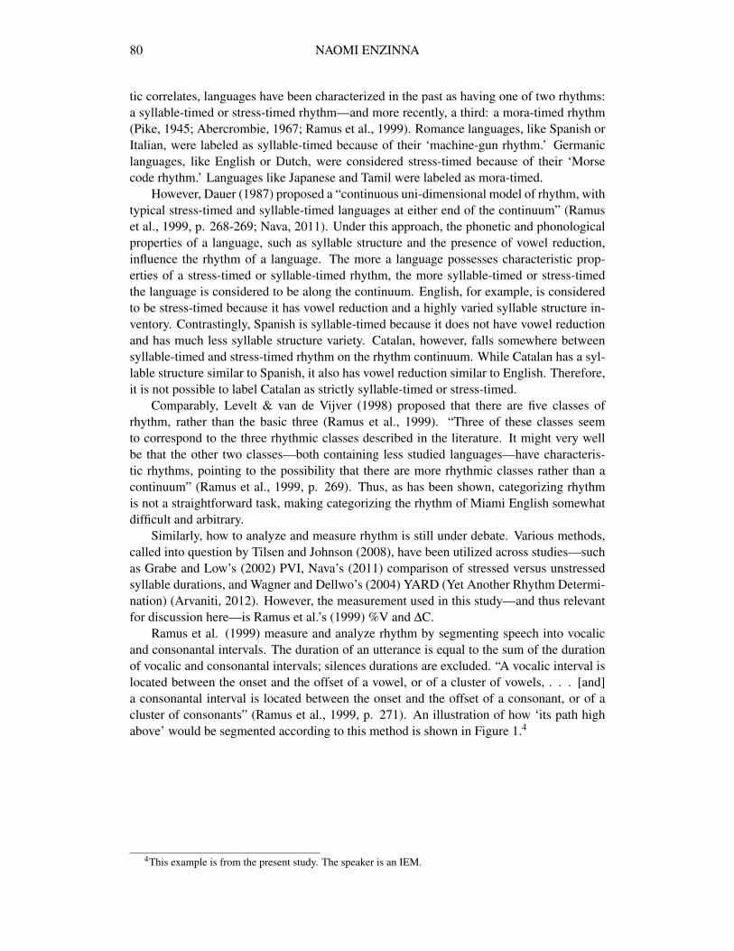
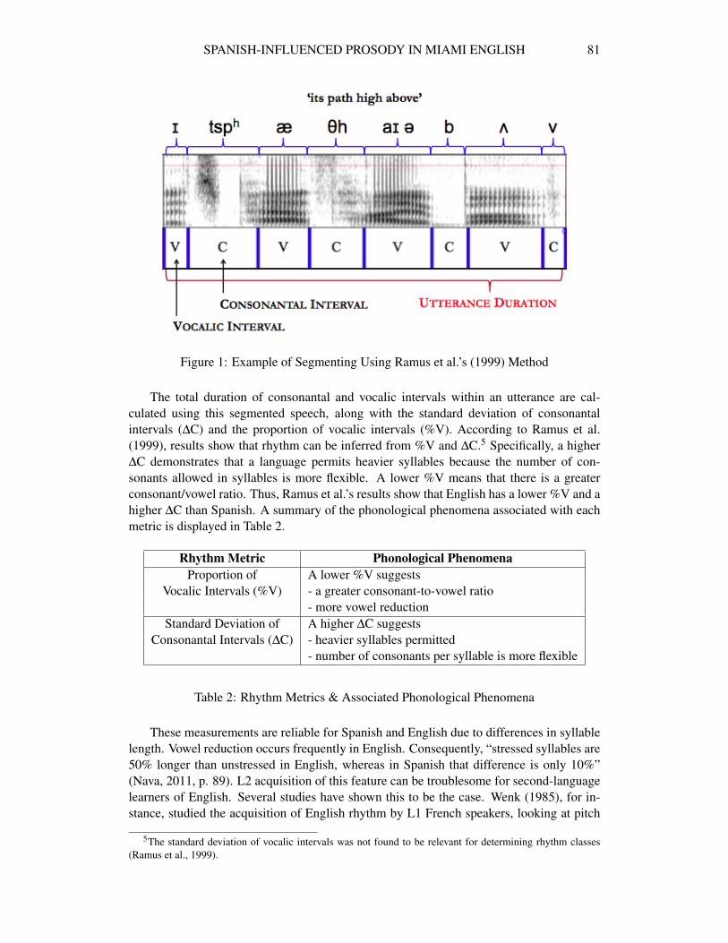
Ramus et al. (1999) measure and analyze rhythm by segmenting speech into vocalicand consonantal intervals. The duration of an utterance is equal to the sum of the durationof vocalic and consonantal intervals; silences durations are excluded. “A vocalic interval islocated between the onset and the offset of a vowel, or of a cluster of vowels, . . . [and]a consonantal interval is located between the onset and the offset of a consonant, or of acluster of consonants” (Ramus et al., 1999, p. 271). An illustration of how ‘its path highabove’ would be segmented according to this method is shown in Figure 1.4

4This example is from the present study. The speaker is an IEM.


Figure 1: Example of Segmenting Using Ramus et al.’s (1999) Method

The total duration of consonantal and vocalic intervals within an utterance are cal-culated using this segmented speech, along with the standard deviation of consonantalintervals (∆C) and the proportion of vocalic intervals (%V). According to Ramus et al.(1999), results show that rhythm can be inferred from %V and ∆C.5 Specifically, a higher∆C demonstrates that a language permits heavier syllables because the number of con-sonants allowed in syllables is more flexible. A lower %V means that there is a greaterconsonant/vowel ratio. Thus, Ramus et al.’s results show that English has a lower %V and ahigher ∆C than Spanish. A summary of the phonological phenomena associated with eachmetric is displayed in Table 2.

Rhythm Metric Phonological PhenomenaProportion of A lower %V suggests

Vocalic Intervals (%V) - a greater consonant-to-vowel ratio- more vowel reduction

Standard Deviation of A higher ∆C suggestsConsonantal Intervals (∆C) - heavier syllables permitted

- number of consonants per syllable is more flexible

Table 2: Rhythm Metrics & Associated Phonological Phenomena

These measurements are reliable for Spanish and English due to differences in syllablelength. Vowel reduction occurs frequently in English. Consequently, “stressed syllables are50% longer than unstressed in English, whereas in Spanish that difference is only 10%”(Nava, 2011, p. 89). L2 acquisition of this feature can be troublesome for second-languagelearners of English. Several studies have shown this to be the case. Wenk (1985), for in-stance, studied the acquisition of English rhythm by L1 French speakers, looking at pitch

5The standard deviation of vocalic intervals was not found to be relevant for determining rhythm classes(Ramus et al., 1999).

82 NAOMI ENZINNA

changes and vowel duration (Nava, 2011). “In describing the L2 acquirer’s ‘rhythmic inter-language,’ he isolates the acquisition of vowel reduction as key in moving from one type ofrhythm to the other” (Nava, 2011, p. 81). Similarly, Adams and Munro (1978) examinedthe production of English stress and rhythm by L1 speakers of English versus L2 speakersof English whose L1 was one of “various Asian languages” (Nava, 2011, p. 82). In theirstudy, they discovered that the non-native speakers of English consistently produced longervowels in unstressed syllables than native English speakers. Similarly, Carter (2005) andGut (2003) found vowel reduction/deletion to be infrequent by L2 learners whose L1 is aSpanish or a Romance language, respectively (Nava, 2011). Thus, it is expected that L2learners of English living in Miami will have trouble adopting English stress patterns andcorresponding vowel reduction.

As shown, categorizing and measuring rhythm are not straightforward tasks. Fortu-nately, for the purposes of this study, it is not imperative to resolve the rhythm debate, asthe goal of this study is not to assess the cross-linguistic validity of Ramus et al.’s (1999)measurement. Rather, this study aims to compare vowel and consonant durations of severalparticipant groups who are all uttering the same passage: a portion of “The Rainbow Pas-sage” in English. Thus, English is being compared to English, not English to Spanish. Forthis purpose, Ramus et al.’s measurement is sufficient.

2.2 Pitch: Native and Non-Native English and Spanish

Pitch differences between IEMs and English speakers from Miami (both MEMs andbilinguals) were noticed after listening to data in this study and to YouTube clips of MiamiEnglish speakers. Specifically, IEMs sounded as if they had greater pitch variation thanMEMs, EBs, and LBs.

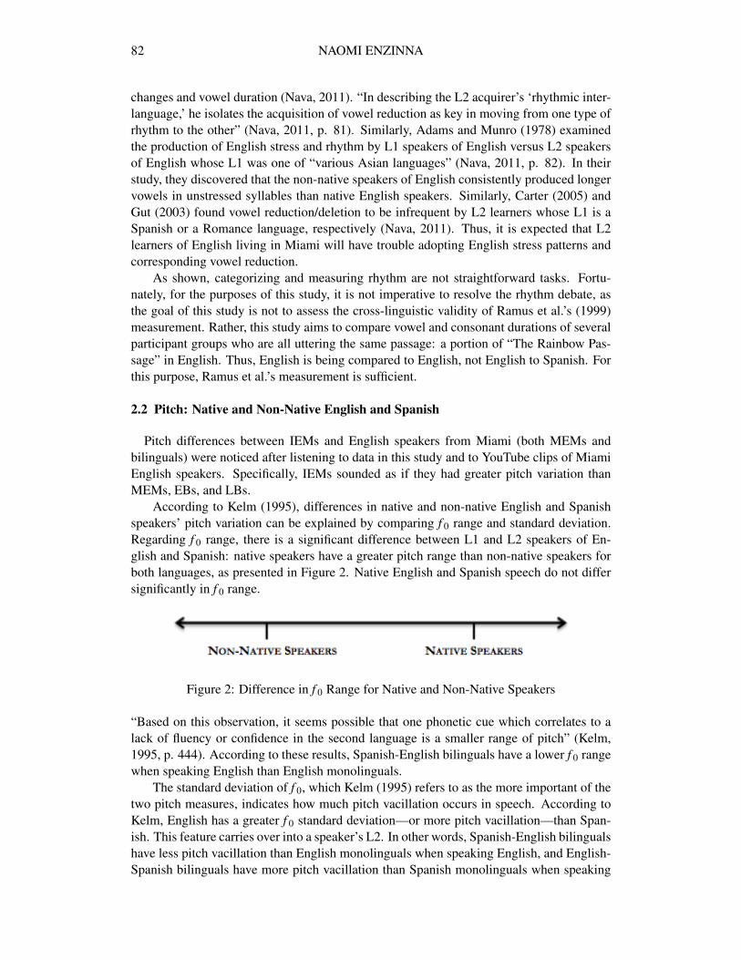
According to Kelm (1995), differences in native and non-native English and Spanishspeakers’ pitch variation can be explained by comparing f 0 range and standard deviation.Regarding f 0 range, there is a significant difference between L1 and L2 speakers of En-glish and Spanish: native speakers have a greater pitch range than non-native speakers forboth languages, as presented in Figure 2. Native English and Spanish speech do not differsignificantly in f 0 range.

Figure 2: Difference in f 0 Range for Native and Non-Native Speakers

“Based on this observation, it seems possible that one phonetic cue which correlates to alack of fluency or confidence in the second language is a smaller range of pitch” (Kelm,1995, p. 444). According to these results, Spanish-English bilinguals have a lower f 0 rangewhen speaking English than English monolinguals.

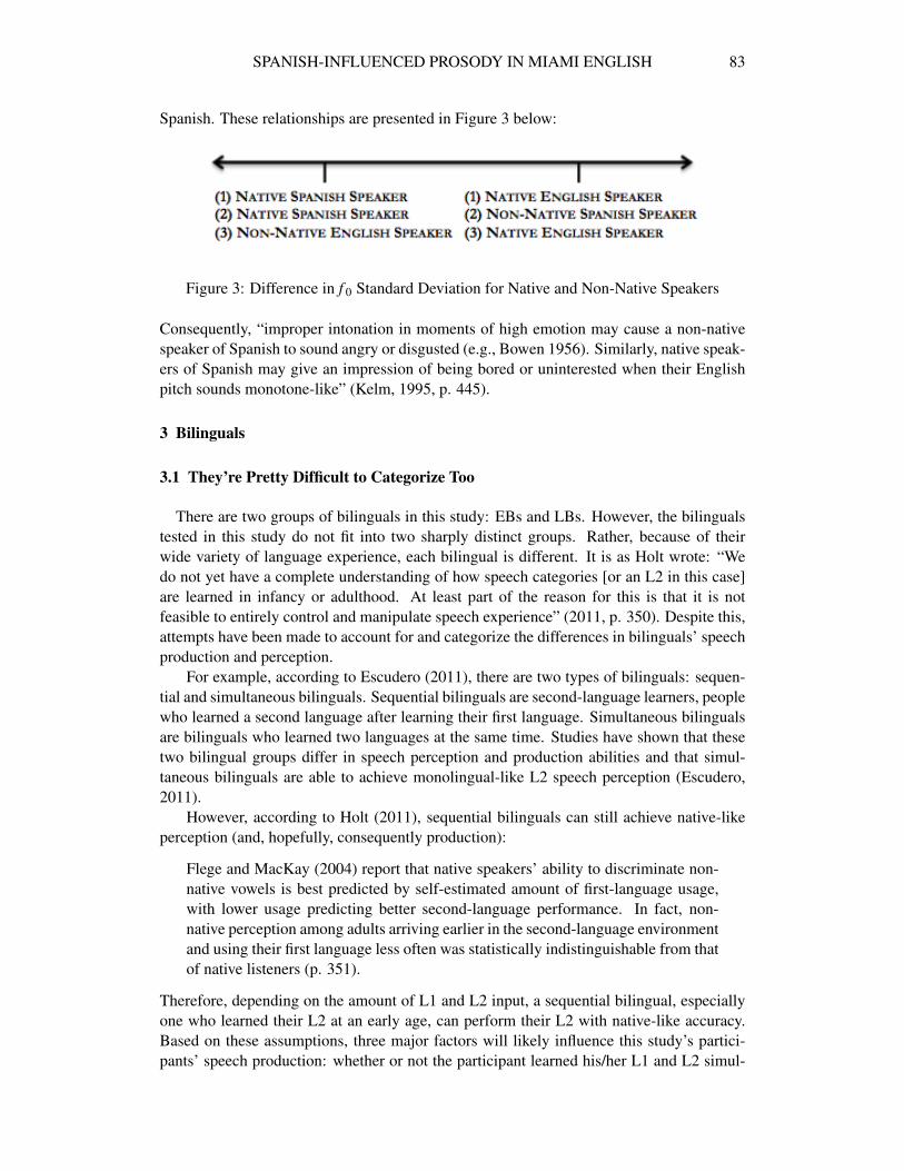
The standard deviation of f 0, which Kelm (1995) refers to as the more important of thetwo pitch measures, indicates how much pitch vacillation occurs in speech. According toKelm, English has a greater f 0 standard deviation—or more pitch vacillation—than Span-ish. This feature carries over into a speaker’s L2. In other words, Spanish-English bilingualshave less pitch vacillation than English monolinguals when speaking English, and English-Spanish bilinguals have more pitch vacillation than Spanish monolinguals when speaking


Spanish. These relationships are presented in Figure 3 below:

Figure 3: Difference in f 0 Standard Deviation for Native and Non-Native Speakers

Consequently, “improper intonation in moments of high emotion may cause a non-nativespeaker of Spanish to sound angry or disgusted (e.g., Bowen 1956). Similarly, native speak-ers of Spanish may give an impression of being bored or uninterested when their Englishpitch sounds monotone-like” (Kelm, 1995, p. 445).

3 Bilinguals

3.1 They’re Pretty Difficult to Categorize Too

There are two groups of bilinguals in this study: EBs and LBs. However, the bilingualstested in this study do not fit into two sharply distinct groups. Rather, because of theirwide variety of language experience, each bilingual is different. It is as Holt wrote: “Wedo not yet have a complete understanding of how speech categories [or an L2 in this case]are learned in infancy or adulthood. At least part of the reason for this is that it is notfeasible to entirely control and manipulate speech experience” (2011, p. 350). Despite this,attempts have been made to account for and categorize the differences in bilinguals’ speechproduction and perception.

For example, according to Escudero (2011), there are two types of bilinguals: sequen-tial and simultaneous bilinguals. Sequential bilinguals are second-language learners, peoplewho learned a second language after learning their first language. Simultaneous bilingualsare bilinguals who learned two languages at the same time. Studies have shown that thesetwo bilingual groups differ in speech perception and production abilities and that simul-taneous bilinguals are able to achieve monolingual-like L2 speech perception (Escudero,2011).

However, according to Holt (2011), sequential bilinguals can still achieve native-likeperception (and, hopefully, consequently production):

Flege and MacKay (2004) report that native speakers’ ability to discriminate non-native vowels is best predicted by self-estimated amount of first-language usage,with lower usage predicting better second-language performance. In fact, non-native perception among adults arriving earlier in the second-language environmentand using their first language less often was statistically indistinguishable from thatof native listeners (p. 351).

Therefore, depending on the amount of L1 and L2 input, a sequential bilingual, especiallyone who learned their L2 at an early age, can perform their L2 with native-like accuracy.Based on these assumptions, three major factors will likely influence this study’s partici-pants’ speech production: whether or not the participant learned his/her L1 and L2 simul-

84 NAOMI ENZINNA

taneously, whether or not the participant learned his/her L2 at an early age, and the amountof L1 versus L2 input the participant receives.

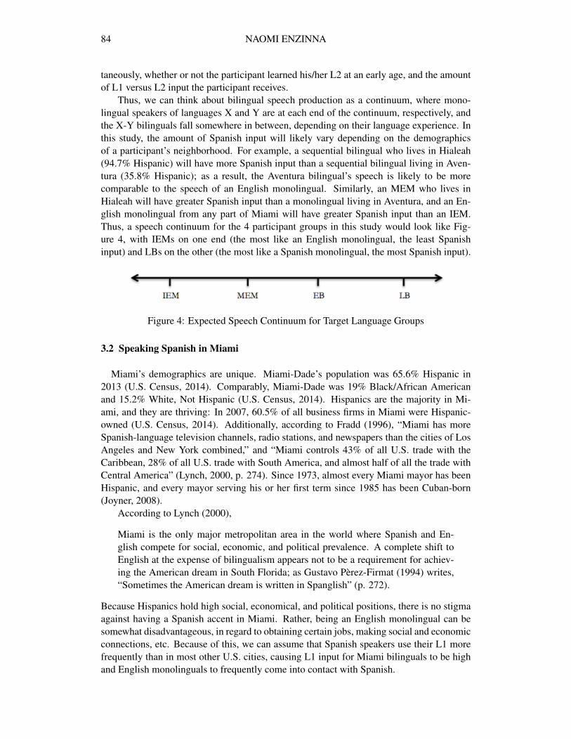
Thus, we can think about bilingual speech production as a continuum, where mono-lingual speakers of languages X and Y are at each end of the continuum, respectively, andthe X-Y bilinguals fall somewhere in between, depending on their language experience. Inthis study, the amount of Spanish input will likely vary depending on the demographicsof a participant’s neighborhood. For example, a sequential bilingual who lives in Hialeah(94.7% Hispanic) will have more Spanish input than a sequential bilingual living in Aven-tura (35.8% Hispanic); as a result, the Aventura bilingual’s speech is likely to be morecomparable to the speech of an English monolingual. Similarly, an MEM who lives inHialeah will have greater Spanish input than a monolingual living in Aventura, and an En-glish monolingual from any part of Miami will have greater Spanish input than an IEM.Thus, a speech continuum for the 4 participant groups in this study would look like Fig-ure 4, with IEMs on one end (the most like an English monolingual, the least Spanishinput) and LBs on the other (the most like a Spanish monolingual, the most Spanish input).

Figure 4: Expected Speech Continuum for Target Language Groups

3.2 Speaking Spanish in Miami

Miami’s demographics are unique. Miami-Dade’s population was 65.6% Hispanic in2013 (U.S. Census, 2014). Comparably, Miami-Dade was 19% Black/African Americanand 15.2% White, Not Hispanic (U.S. Census, 2014). Hispanics are the majority in Mi-ami, and they are thriving: In 2007, 60.5% of all business firms in Miami were Hispanic-owned (U.S. Census, 2014). Additionally, according to Fradd (1996), “Miami has moreSpanish-language television channels, radio stations, and newspapers than the cities of LosAngeles and New York combined,” and “Miami controls 43% of all U.S. trade with theCaribbean, 28% of all U.S. trade with South America, and almost half of all the trade withCentral America” (Lynch, 2000, p. 274). Since 1973, almost every Miami mayor has beenHispanic, and every mayor serving his or her first term since 1985 has been Cuban-born(Joyner, 2008).

According to Lynch (2000),

Miami is the only major metropolitan area in the world where Spanish and En-glish compete for social, economic, and political prevalence. A complete shift toEnglish at the expense of bilingualism appears not to be a requirement for achiev-ing the American dream in South Florida; as Gustavo Pèrez-Firmat (1994) writes,“Sometimes the American dream is written in Spanglish” (p. 272).

Because Hispanics hold high social, economical, and political positions, there is no stigmaagainst having a Spanish accent in Miami. Rather, being an English monolingual can besomewhat disadvantageous, in regard to obtaining certain jobs, making social and economicconnections, etc. Because of this, we can assume that Spanish speakers use their L1 morefrequently than in most other U.S. cities, causing L1 input for Miami bilinguals to be highand English monolinguals to frequently come into contact with Spanish.


4 The Study

4.1 Research Questions

This study aims to answer the following questions:

1. Has the rhythm of MEM speech been influenced by the high number of Spanish-speakers in Miami? If so,

(a) How does rhythm of MEM speech compare to the rhythm of IEM speech?

(b) How does the rhythm of MEM speech compare to the rhythm of EB and LBspeech?

2. What mechanisms are responsible for whether or not MEMs or EBs acquire Spanish-influenced English rhythm? More specifically,

(a) Is a participant’s rhythm influenced by living in a Miami neighborhood with ahigher or lower Hispanic demographic?

(b) Does having Spanish-speaking parents make an MEM more likely to use a Spanish-influenced speech rhythm?

(c) Are simultaneous bilinguals less likely than sequential bilinguals to use Spanish-influenced rhythm in their English speech?

3. Has the pitch of MEM speech been influenced by the high number of Spanish-speakersin Miami? If so,

(a) How does pitch in MEM speech compare to pitch in IEM speech?6

4.2 Hypotheses & Predictions

In response to the research questions above, I hypothesize and predict the following:

1. Hypothesis: The rhythm of English spoken in Miami has been influenced by the highnumber of Spanish-speakers in South Florida.

(a) MEM rhythm is more characteristic of Spanish than IEM rhythm.

(b) MEM rhythm is less characteristic of Spanish than EB and LB rhythm. LB rhythmis more characteristic of Spanish than EB rhythm.

Prediction: Using Ramus et al.’s (1999) rhythm metrics,

(a) IEMs have a lower %V and higher ∆C7 than MEMs (and EBs, LBs).

(b) MEMs have a lower %V and higher ∆C than EBs and LBs, and LBs have a higher%V and the lower ∆C than MEMs and EBs (and IEMs).

6A comparison between MEMs and EBs/LBs is not possible because there are not enough male EBs orfemale LBs to do an adequate comparison. However, Kelm’s (1995) results still allow for a prediction to bemade about EB and LB pitch, which is that both groups have a lower f 0 range and standard deviation thanIEMs.

7Since English is being compared between groups, it was predicted that ∆C may not be a factor at all.

86 NAOMI ENZINNA

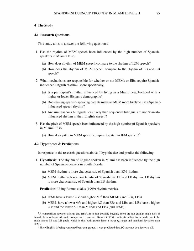
In Figure 5, a graph from Ramus et al.’s (1999) study is shown; on this graph, a pre-diction for MEMs’ %V and ∆C is shown in red. I expect the results of IEMs to becomparable to that of Ramus et al.’s EN (English) group and the results of my EB andLB groups to fall between MEM and SP (Spanish), depending on their L1/L2 languageexperience.

Figure 5: Altered Ramus et al. (1999) Graph, Showing MEM Prediction

2. Hypothesis: MEMs and EBs with greater Spanish input have a Spanish-influencedEnglish rhythm. More specifically,

(a) Participants residing in Miami neighborhoods with a higher Hispanic demographichave a Spanish-influenced rhythm.

(b) MEMs with Spanish-speaking parents have a Spanish-influenced rhythm.(c) Sequential EBs’ rhythm is more similar to Spanish than simultaneous EBs’ rhythm.

Prediction: Using Ramus et al.’s (1999) rhythm metrics, MEMs and EBs with greaterSpanish input have a higher %V and lower ∆C than those with less Spanish input. Inother words,

(a) Participants from a neighborhood with a high Hispanic demographic have a higher%V and lower ∆C than participants from a neighborhood with a low Hispanicpopulation.

(b) MEMs with Spanish-speaking parents have a higher %V and lower ∆C than MEMswith English-speaking parents.

(c) Sequential EBs have a higher %V and lower ∆C than simultaneous EBs.

This prediction is illustrated with the continuum (arrow) in Figure 6; participant groupson the left have less Spanish input than their corresponding group on the right.


Figure 6: Speech Continuum of Amount of Spanish Input

3. Hypothesis: The pitch of English spoken in Miami has been influenced by the highnumber of Spanish-speakers in South Florida.

(a) MEM pitch is more characteristic of Spanish-English bilingual pitch than IEMpitch.

Prediction: Using Kelm’s (1995) pitch metrics,

(a) MEMs have a lower f 0 range and standard deviation than IEMs.

This prediction is illustrated with the continuum (arrow) in Figure 7.

Figure 7: Comparison of MEM and IEM f 0 Range and Standard Deviation

4.3 Methodology

4.3.1 Participants

For each of the following 4 language groups, 10 participants were recorded: MEMs,IEMs, EBs, and LBs. A language background questionnaire was used to determine eachparticipant’s language group, as well as his/her Miami neighborhood, parents’ language(s),L2 age of acquisition (if applicable), relative importance of English to Spanish, and more.Descriptions of all groups are provided in Table 3.

All participants were between the ages of 18 and 30,8 including both males and females.Participants were recruited through advertisements at local universities, an advertisementwebsite,9 and the principal investigator’s social groups.

4.3.2 Materials & Procedure

The materials were presented to participants in the following order: 10 interview ques-tions, “The North Wind and the Sun” (of Aesop’s Fables), “The Rainbow Passage,” 15

8Testing within this age range helps to ensure that any results used as evidence for or against the existence ofan emerging Miami dialect are characteristic of a younger generation of Miami-English speakers. Additionally,focusing on younger speakers means major shifts in their demographics are less likely.

9Craigslist.

88 NAOMI ENZINNA

Abbrev. Participant Group Description

EB Early Spanish-English BilingualLived in Miami majority of life;Speaks Spanish, English;Learned English before age 10

EBH from high Hispanic population area Miami neighborhood>50% HispanicEBL from low Hispanic population area Miami neighborhood<50 % Hispanic

SEQ EB Sequential Early Bilingual Learned Spanish before EnglishSIM EB Simultaneous Early Bilingual Learned Spanish and English from birth

IEM Ithaca English Monolingual

Lived in Ithaca 10+ years,Speaks English,Represents English monolingual groupwith low Spanish contact

LB Late Spanish-English BilingualBorn outside USA;Speaks Spanish, English;Learned English after age 10

MEM Miami English MonolingualLived in Miami majority of life,Speaks English

MEME with English-speaking parents Parents speak EnglishMEMS with Spanish-speaking parents Parents speak Spanish

MEMH from high Hispanic population area Miami neighborhood>50% HispanicMEML from low Hispanic population area Miami neighborhood<50% Hispanic

Table 3: Participant Group Abbreviations

sentences from Arvaniti’s (2012) study, a word list, and a language-background question-naire. When presented with the reading passages, sentences, and word list, participantswere asked to read the materials once to themselves and then once aloud. With the excep-tion of the questionnaire, all participant interactions with the materials were audio recorded.At the end of the procedure, participants received $10 for approximately 30 minutes of par-ticipation.

Of the materials, the language-background questionnaire and the first eight lines of“The Rainbow Passage” were used in the present analysis; these eight lines are presentedbelow:

When the sunlight strikes raindrops in the air, they act as a prism and form a rain-bow. The rainbow is a division of white light into many beautiful colors. Thesetake the shape of a long round arch, with its path high above, and its two ends ap-parently beyond the horizon. There is, according to legend, a boiling pot of gold atone end. People look, but no one ever finds it. When a man looks for somethingbeyond his reach, his friends say he is looking for the pot of gold at the end of the


rainbow. Throughout the centuries people have explained the rainbow in variousways. Some have accepted it as a miracle without physical explanation.

4.3.3 Analysis

Each participant’s results were segmented into vocalic and consonantal intervals, si-lences, and disfluencies in Praat; syllabic consonants were labeled as vowels and disfluencydurations were not counted in duration totals.10 Then, the resulting text grids were readand analyzed in Matlab. Figure 8, repeated from Section 2.1, illustrates how ‘its path highabove’ was segmented in this study.

Figure 8: Example of Segmenting Using Ramus et al.’s (1999) Method

The data were analyzed in two ways: by-subject and by-utterance. In the by-subjectanalysis, all consonant and vowel durations were added to a single total duration, of whichthe proportion of vocalic intervals (%V) and the standard deviation of consonantal intervals(∆C) were calculated. In this analysis, each participant had only one %V and ∆C value forhis/her entire passage reading (all eight lines of “The Rainbow Passage”).

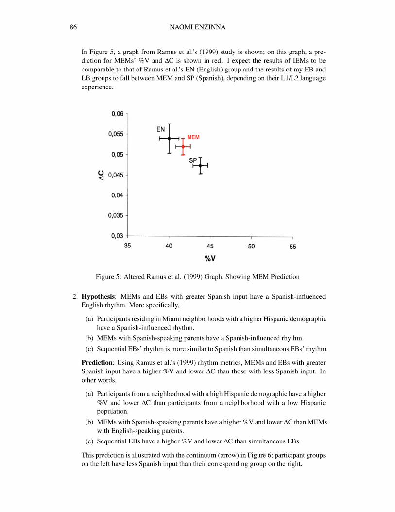
In the by-utterance analysis, vocalic and consonantal interval durations were added tothe total duration of an utterance until there was a silence of 200 ms or greater. Accordingto Thomas and Carter (2006), “Butterworth (1980) notes that 200 ms has become a standardminimum threshold for a pause in studies of pauses” (p. 340). Assuming this standard, theduration of a new utterance began to be calculated after any 200+ ms pause, resulting inmultiple %V and ∆C values for each participant. For example, Figure 9 shows a stretch ofspeech where a speaker pauses (labeled ‘S’) for more than 200 ms (476 ms). This silencefalls between ‘The rainbow is a division of white light into many beautiful colors’ and‘These take the shape of a long round arch . . .’ The consonantal and vocalic intervalsbefore that silence (and after the preceding silence) are equal to one total utterance duration,

10Disfluency durations were not included to ensure that participants’ recordings included the same exactstretch of speech.

90 NAOMI ENZINNA

and the intervals after that silence (and before the next silence) are equal to another totalutterance duration.

Figure 9: Example of Silence Creating New Total Utterance Duration

For the pitch analysis, pitch contours were obtained for each utterance with the RAPT(Robust Automated Pitch Tracking) algorithm (Talkin, 1995), implemented in the Voiceboxtoolbox (Brookes, 1997) for Matlab. In order to obtain more accurate pitch contours, f 0 out-liers were excluded and contours were fit with a smoothing spine. Additionally, utterancesless than 500 ms were removed from the analysis.

5 Results

The results in this section suggest that MEM prosody—in regards to rhythm and pitch—is influenced by Spanish. More specifically, MEMs have a greater %V and a lower f 0range and standard deviation than IEMs, both which are characteristic of Spanish and/orSpanish-English bilingual speech. Additionally, results suggest that MEMs (and EBs) withless Spanish input are leading this trend.

Section 5.1 presents the distribution of consonantal and vocalic intervals, silences, andtotal durations across participant groups. Section 5.2 presents the results by linguistic (par-ticipant) group. Section 5.3 examines the influence of parent language on MEM results.Section 5.4 examines the influence of neighborhood demographics on MEM and EB re-sults. Section 5.5 examines the difference between simultaneous and sequential EB rhythm.Section 5.6 provides evidence of LB participants’ L2 production difficulties. Section 5.7examines the influence of speech rate on %V and ∆C. Last, section 5.7 presents pitch re-sults.

5.1 Interval Distribution

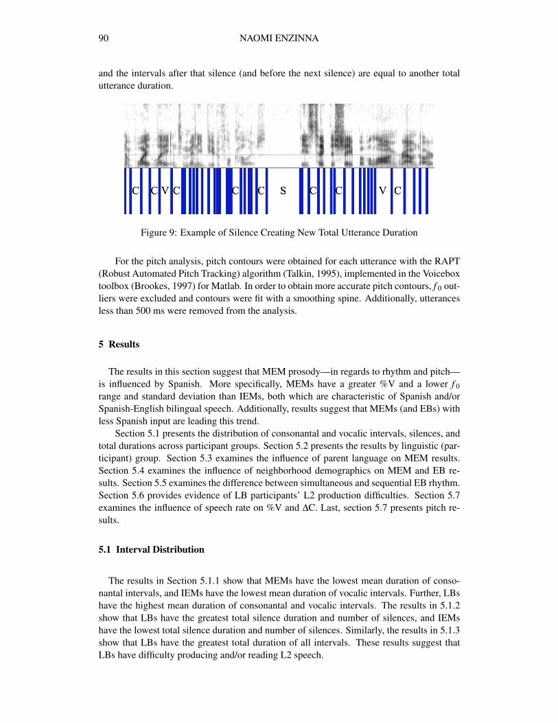
The results in Section 5.1.1 show that MEMs have the lowest mean duration of conso-nantal intervals, and IEMs have the lowest mean duration of vocalic intervals. Further, LBshave the highest mean duration of consonantal and vocalic intervals. The results in 5.1.2show that LBs have the greatest total silence duration and number of silences, and IEMshave the lowest total silence duration and number of silences. Similarly, the results in 5.1.3show that LBs have the greatest total duration of all intervals. These results suggest thatLBs have difficulty producing and/or reading L2 speech.


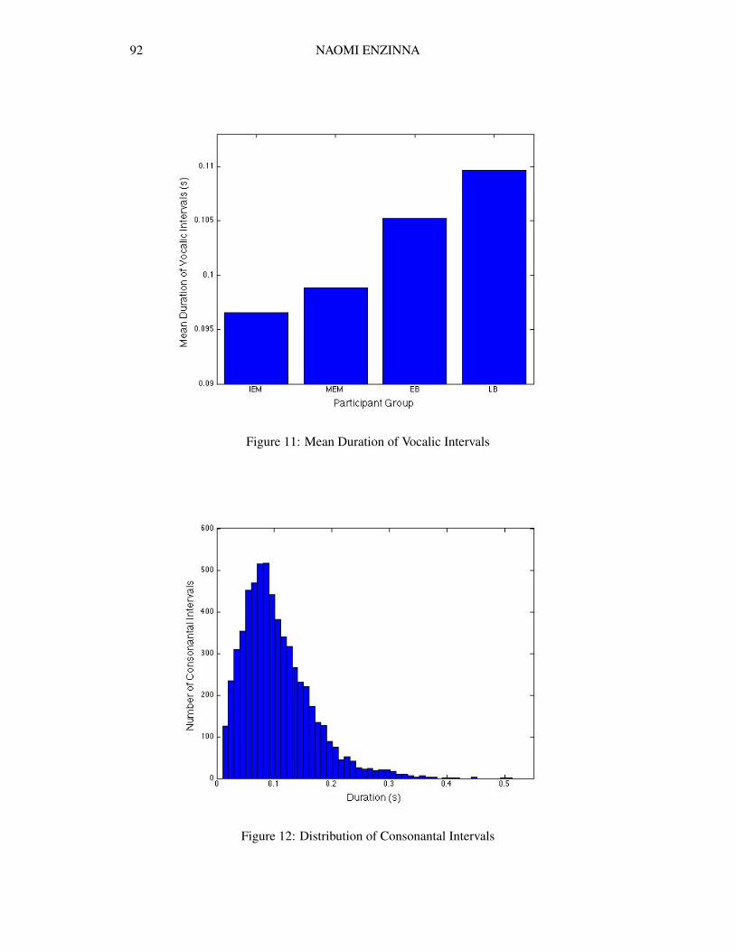
5.1.1 Consonantal and Vocalic Interval Means

The mean duration (in seconds), the standard deviation, and the number of consonantaland vocalic intervals for all participants and for each participant group are presented inTable 4:

Consonantal VocalicALL 0.104 (0.060, 6096) 0.099 (0.059, 6224)IEM 0.102 (0.057, 1495) 0.094 (0.057, 1516)

MEM 0.097 (0.057, 1499) 0.095 (0.056, 1556)EB 0.104 (0.057, 1552) 0.101 (0.058, 1576)LB 0.112 (0.065, 1550) 0.105 (0.062, 1576)

Table 4: Interval Means, Standard Deviation, Number of Tokens (Mean (St.Dev., N))

These results are illustrated in Figures 10 and 11.

Figure 10: Mean Duration of Consonantal Intervals

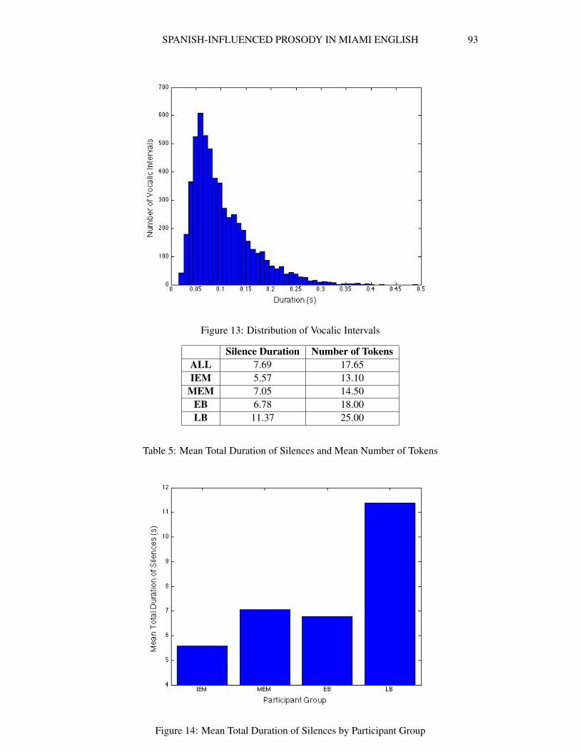
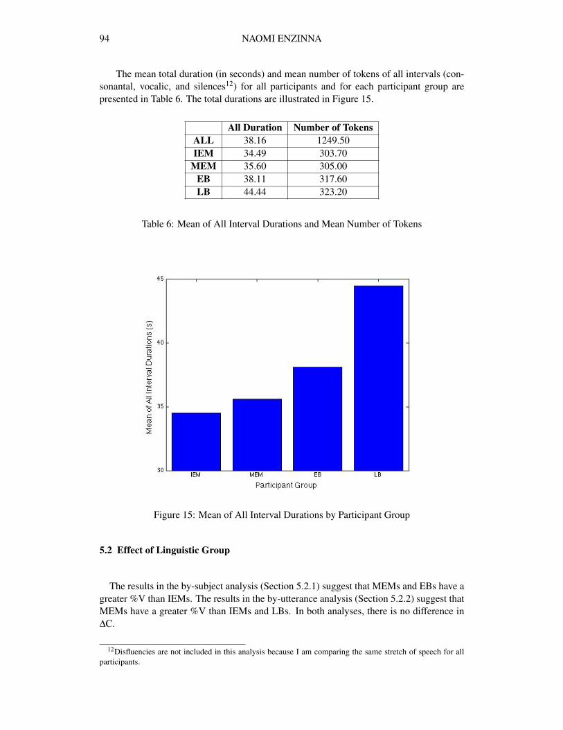
The distribution of consonantal and vocalic intervals for all participants are shown inFigures 12 and 13.

5.1.2 Mean Silence & All Interval Durations

The mean total duration of silences (in seconds) and the mean number of silences11 forall participants and for each participant group are presented in Table 5. The total durationmeans are illustrated in Figure 14.

11The mean and token values do not include the silence before or after the participants read the passage.

92 NAOMI ENZINNA

Figure 11: Mean Duration of Vocalic Intervals

Figure 12: Distribution of Consonantal Intervals


Figure 13: Distribution of Vocalic Intervals

Silence Duration Number of TokensALL 7.69 17.65IEM 5.57 13.10

MEM 7.05 14.50EB 6.78 18.00LB 11.37 25.00

Table 5: Mean Total Duration of Silences and Mean Number of Tokens

Figure 14: Mean Total Duration of Silences by Participant Group

94 NAOMI ENZINNA

The mean total duration (in seconds) and mean number of tokens of all intervals (con-sonantal, vocalic, and silences12) for all participants and for each participant group arepresented in Table 6. The total durations are illustrated in Figure 15.

All Duration Number of TokensALL 38.16 1249.50IEM 34.49 303.70

MEM 35.60 305.00EB 38.11 317.60LB 44.44 323.20

Table 6: Mean of All Interval Durations and Mean Number of Tokens

Figure 15: Mean of All Interval Durations by Participant Group

5.2 Effect of Linguistic Group

The results in the by-subject analysis (Section 5.2.1) suggest that MEMs and EBs have agreater %V than IEMs. The results in the by-utterance analysis (Section 5.2.2) suggest thatMEMs have a greater %V than IEMs and LBs. In both analyses, there is no difference in∆C.

12Disfluencies are not included in this analysis because I am comparing the same stretch of speech for allparticipants.


5.2.1 Effect of Linguistic Group by Subject

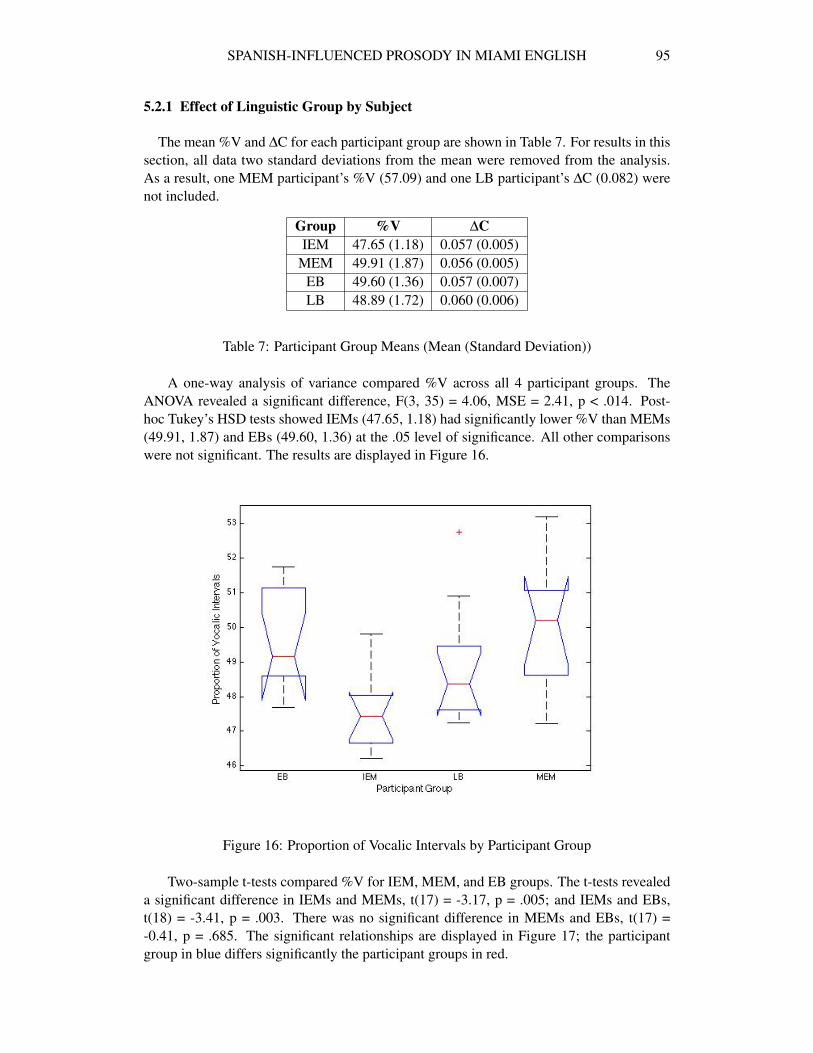
The mean %V and ∆C for each participant group are shown in Table 7. For results in thissection, all data two standard deviations from the mean were removed from the analysis.As a result, one MEM participant’s %V (57.09) and one LB participant’s ∆C (0.082) werenot included.

Group %V ∆CIEM 47.65 (1.18) 0.057 (0.005)

MEM 49.91 (1.87) 0.056 (0.005)EB 49.60 (1.36) 0.057 (0.007)LB 48.89 (1.72) 0.060 (0.006)

Table 7: Participant Group Means (Mean (Standard Deviation))

A one-way analysis of variance compared %V across all 4 participant groups. TheANOVA revealed a significant difference, F(3, 35) = 4.06, MSE = 2.41, p < .014. Post-hoc Tukey’s HSD tests showed IEMs (47.65, 1.18) had significantly lower %V than MEMs(49.91, 1.87) and EBs (49.60, 1.36) at the .05 level of significance. All other comparisonswere not significant. The results are displayed in Figure 16.

Figure 16: Proportion of Vocalic Intervals by Participant Group

Two-sample t-tests compared %V for IEM, MEM, and EB groups. The t-tests revealeda significant difference in IEMs and MEMs, t(17) = -3.17, p = .005; and IEMs and EBs,t(18) = -3.41, p = .003. There was no significant difference in MEMs and EBs, t(17) =-0.41, p = .685. The significant relationships are displayed in Figure 17; the participantgroup in blue differs significantly the participant groups in red.

96 NAOMI ENZINNA

Figure 17: Significant Relationships for %V by Participant Group

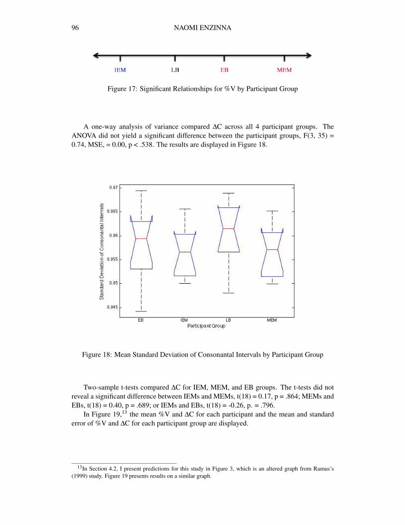
A one-way analysis of variance compared ∆C across all 4 participant groups. TheANOVA did not yield a significant difference between the participant groups, F(3, 35) =0.74, MSE, = 0.00, p < .538. The results are displayed in Figure 18.

Figure 18: Mean Standard Deviation of Consonantal Intervals by Participant Group

Two-sample t-tests compared ∆C for IEM, MEM, and EB groups. The t-tests did notreveal a significant difference between IEMs and MEMs, t(18) = 0.17, p = .864; MEMs andEBs, t(18) = 0.40, p = .689; or IEMs and EBs, t(18) = -0.26, p. = .796.

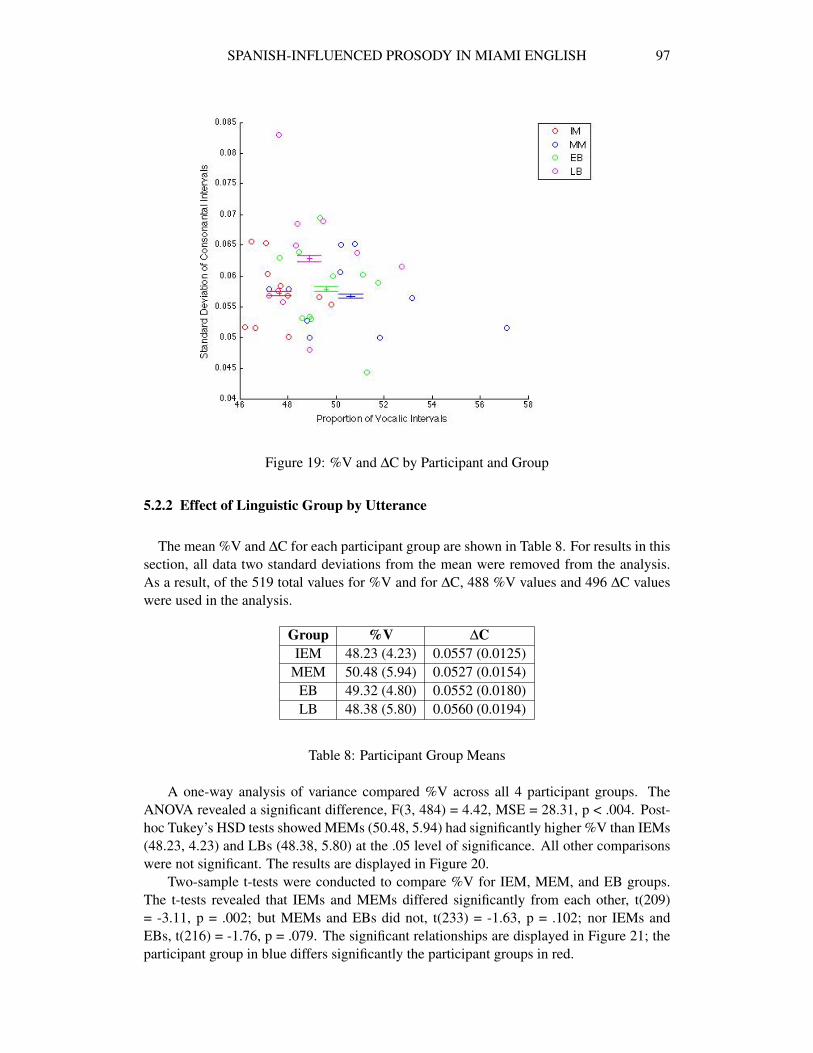
In Figure 19,13 the mean %V and ∆C for each participant and the mean and standarderror of %V and ∆C for each participant group are displayed.

13In Section 4.2, I present predictions for this study in Figure 3, which is an altered graph from Ramus’s(1999) study. Figure 19 presents results on a similar graph.


Figure 19: %V and ∆C by Participant and Group

5.2.2 Effect of Linguistic Group by Utterance

The mean %V and ∆C for each participant group are shown in Table 8. For results in thissection, all data two standard deviations from the mean were removed from the analysis.As a result, of the 519 total values for %V and for ∆C, 488 %V values and 496 ∆C valueswere used in the analysis.

Group %V ∆CIEM 48.23 (4.23) 0.0557 (0.0125)

MEM 50.48 (5.94) 0.0527 (0.0154)EB 49.32 (4.80) 0.0552 (0.0180)LB 48.38 (5.80) 0.0560 (0.0194)

Table 8: Participant Group Means

A one-way analysis of variance compared %V across all 4 participant groups. TheANOVA revealed a significant difference, F(3, 484) = 4.42, MSE = 28.31, p < .004. Post-hoc Tukey’s HSD tests showed MEMs (50.48, 5.94) had significantly higher %V than IEMs(48.23, 4.23) and LBs (48.38, 5.80) at the .05 level of significance. All other comparisonswere not significant. The results are displayed in Figure 20.

Two-sample t-tests were conducted to compare %V for IEM, MEM, and EB groups.The t-tests revealed that IEMs and MEMs differed significantly from each other, t(209)= -3.11, p = .002; but MEMs and EBs did not, t(233) = -1.63, p = .102; nor IEMs andEBs, t(216) = -1.76, p = .079. The significant relationships are displayed in Figure 21; theparticipant group in blue differs significantly the participant groups in red.

98 NAOMI ENZINNA

Figure 20: Proportion of Vocalic Intervals by Participant Group


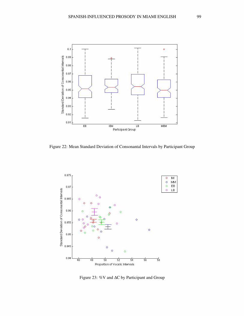
A one-way analysis of variance was conducted to compare ∆C across all 4 participantgroups. The ANOVA did not yield a significant difference between the participant groups,F(3, 492) = 0.99, MSE, = 0.00, p < .397. The results are displayed in Figure 22.

Two-sample t-tests were conducted to compare ∆C for IEM, MEM, and EB groups.The t-tests did not reveal a significant difference between IEMs and MEMs, t(212) = 1.55,p = .120; MEMs and EBs, t(242) = 1.17, p = .242; or IEMs and EBs, t(222) = 0.23, p =.813.

In Figure 23, the mean %V and ∆C for each participant and the mean and standard errorof %V and ∆C for each participant group are displayed.

5.3 Effect of Parents’ Language

Half (5) of the MEM participants’ parents are Spanish-English bilinguals, while the re-maining half are English monolinguals. Of interest is whether or not this influences MEMs’%V and ∆C results. In the following two subsections, MEM participants are split into twogroups—MEMEs and MEMSs14—and compared with IEMs and EBs.

The by-subject (Section 5.3.1) results suggest that parent language does not influenceMEMs’ %V or ∆C; both MEMEs and MEMSs have a greater %V than IEMs. However, the

14See Table 3 for more details.


Figure 22: Mean Standard Deviation of Consonantal Intervals by Participant Group

Figure 23: %V and ∆C by Participant and Group

100 NAOMI ENZINNA

by-utterance results suggest that parent language may be an influencing factor for MEMs’%V, but not for ∆C. Specifically, MEMEs have a greater %V than IEMs and EBs, butMEMSs do not.

5.3.1 Effect of Parents’ Language by Subject

The mean %V and ∆C for each participant group are shown in Table 9. For results in thissection, all data two standard deviations from the mean were removed from the analysis.As a result, one MEME participant’s %V (57.09) was not included.

Group %V ∆CIEM 47.65 (1.18) 0.057 (0.005)

MEME 50.00 (1.97) 0.057 (0.006)MEMS 49.83 (2.02) 0.056 (0.005)

EB 49.60 (1.36) 0.057 (0.007)


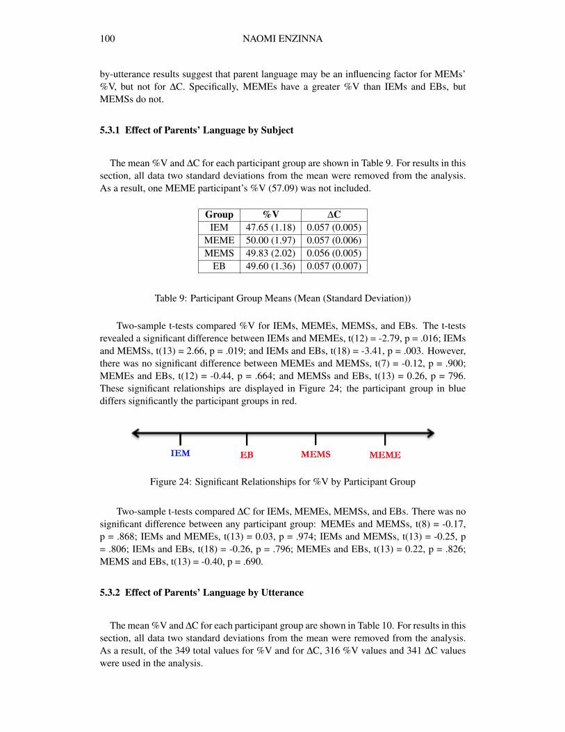
Two-sample t-tests compared %V for IEMs, MEMEs, MEMSs, and EBs. The t-testsrevealed a significant difference between IEMs and MEMEs, t(12) = -2.79, p = .016; IEMsand MEMSs, t(13) = 2.66, p = .019; and IEMs and EBs, t(18) = -3.41, p = .003. However,there was no significant difference between MEMEs and MEMSs, t(7) = -0.12, p = .900;MEMEs and EBs, t(12) = -0.44, p = .664; and MEMSs and EBs, t(13) = 0.26, p = 796.These significant relationships are displayed in Figure 24; the participant group in bluediffers significantly the participant groups in red.


Two-sample t-tests compared ∆C for IEMs, MEMEs, MEMSs, and EBs. There was nosignificant difference between any participant group: MEMEs and MEMSs, t(8) = -0.17,p = .868; IEMs and MEMEs, t(13) = 0.03, p = .974; IEMs and MEMSs, t(13) = -0.25, p= .806; IEMs and EBs, t(18) = -0.26, p = .796; MEMEs and EBs, t(13) = 0.22, p = .826;MEMS and EBs, t(13) = -0.40, p = .690.

5.3.2 Effect of Parents’ Language by Utterance



Group %V ∆CIEM 48.23 (4.23) 0.055 (0.012)

MEME 51.52 (5.80) 0.052 (0.015)MEMS 49.66 (5.96) 0.053 (0.015)

EB 49.32 (4.80) 0.055 (0.018)


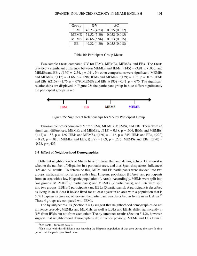
Two-sample t-tests compared %V for IEMs, MEMEs, MEMSs, and EBs. The t-testsrevealed a significant difference between MEMEs and IEMs, t(145) = -3.91, p <.000; andMEMEs and EBs, t(169) = -2.54, p = .011. No other comparisons were significant: MEMEsand MEMSs, t(112) = -1.66, p = .098; IEMs and MEMSs, t(159) = 1.78, p = .076; IEMsand EBs, t(216) = -1.76, p = .079; MEMSs and EBs, t(183) = 0.41, p = .676. The significantrelationships are displayed in Figure 25; the participant group in blue differs significantlythe participant groups in red.


Two-sample t-tests compared ∆C for IEMs, MEMEs, MEMSs, and EBs. There were nosignificant differences: MEMEs and MEMEs, t(115) = 0.38, p = .704; IEMs and MEMEs,t(147) = 1.53, p = .126; IEMs and MEMSs, t(160) = -1.16, p = .245; IEMs and EBs, t(222)= 0.23, p = .813; MEMEs and EBs, t(177) = 1.09, p = .276; MEMSs and EBs, t(190) =-0.78, p = .435.

5.4 Effect of Neighborhood Demographics

Different neighborhoods of Miami have different Hispanic demographics. Of interest iswhether the number of Hispanics in a particular area, and thus Spanish speakers, influences%V and ∆C results. To determine this, MEM and EB participants were divided into twogroups: participants from an area with a high Hispanic population (H Area) and participantsfrom an area with a low Hispanic population (L Area). Accordingly, MEMs were split intotwo groups: MEMHs15 (3 participants) and MEMLs (7 participants), and EBs were splitinto two groups: EBHs (5 participants) and EBLs (5 participants). A participant is describedas living in an H Area if he/she lived for at least a year in an area with a population that is50% Hispanic or greater; otherwise, the participant was described as living in an L Area.16

These 4 groups are compared with IEMs.The by-subject results (Section 5.4.1) suggest that neighborhood demographics do not

influence prosody; MEMLs and MEMHs, as well as EBLs and EBHs, differ significantly in%V from IEMs but not from each other. The by-utterance results (Section 5.4.2), however,suggest that neighborhood demographics do influence prosody; MEMs and EBs from L

15See Table 3 for more details.16One issue with this division is not knowing the Hispanic population of that area during the specific time

period that the participant lived there.

102 NAOMI ENZINNA

Areas have significantly greater %V than MEMs and EBs from H Areas, as well as IEMs.Additionally, the by-utterance results show that MEMLs have a significantly lower ∆C thanIEMs.

5.4.1 Effect of Neighborhood Demographics by Subject

The mean %V and ∆C for each participant group are shown in Table 11. For results in thissection, all data two standard deviations from the mean were removed from the analysis.As a result, one MEML participant’s %V (57.09).

Group %V ∆CIEM 47.65 (1.18) 0.057 (0.005)

MEML 49.62 (1.64) 0.055 (0.005)MEMH 50.48 (2.57) 0.059 (0.004)

EBL 49.89 (1.53) 0.057 (0.009)EBH 49.31 (1.28) 0.057 (0.004)


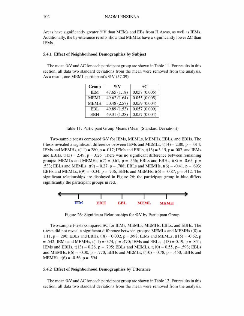
Two-sample t-tests compared %V for IEMs, MEMLs, MEMHs, EBLs, and EBHs. Thet-tests revealed a significant difference between IEMs and MEMLs, t(14) = 2.80, p = .014;IEMs and MEMHs, t(11) = 280, p = .017; IEMs and EBLs, t(13) = 3.15, p = .007, and IEMsand EBHs, t(13) = 2.49, p = .026. There was no significant difference between remaininggroups: MEMLs and MEMHs, t(7) = 0.61, p = .556; EBLs and EBHs, t(8) = -0.65, p =.533; EBLs and MEMLs, t(9) = 0.27, p = .788; EBLs and MEMHs, t(6) = -0.41, p = .693;EBHs and MEMLs, t(9) = -0.34, p = .736; EBHs and MEMHs, t(6) = -0.87, p = .412. Thesignificant relationships are displayed in Figure 26; the participant group in blue differssignificantly the participant groups in red.


Two-sample t-tests compared ∆C for IEMs, MEMLs, MEMHs, EBLs, and EBHs. Thet-tests did not reveal a significant difference between groups: MEMLs and MEMHs t(8) =1.11, p = .296; EBLs and EBHs, t(8) = 0.002, p = .998; IEMs and MEMLs, t(15) = -0.62, p= .542; IEMs and MEMHs, t(11) = 0.74, p = .470; IEMs and EBLs, t(13) = 0.19, p = .851;IEMs and EBHs, t(13) = 0.26, p = .795; EBLs and MEMLs, t(10) = 0.55, p= .593; EBLsand MEMHs, t(6) = -0.30, p = .770; EBHs and MEMLs, t(10) = 0.78, p = .450; EBHs andMEMHs, t(6) = -0.56, p = .594.

5.4.2 Effect of Neighborhood Demographics by Utterance

The mean %V and ∆C for each participant group are shown in Table 12. For results in thissection, all data two standard deviations from the mean were removed from the analysis.


As a result, of the 349 total values for %V and for ∆C, 316 %V values and 341 ∆C valueswere used in the analysis.

Group %V ∆CIEM 48.23 (4.23) 0.055 (0.012)

MEML 51.31 (5.44) 0.051 (0.015)MEMH 49.19 (6.49) 0.055 (0.014)

EBL 50.22 (4.87) 0.055 (0.018)EBH 48.38 (4.59) 0.055 (0.018)


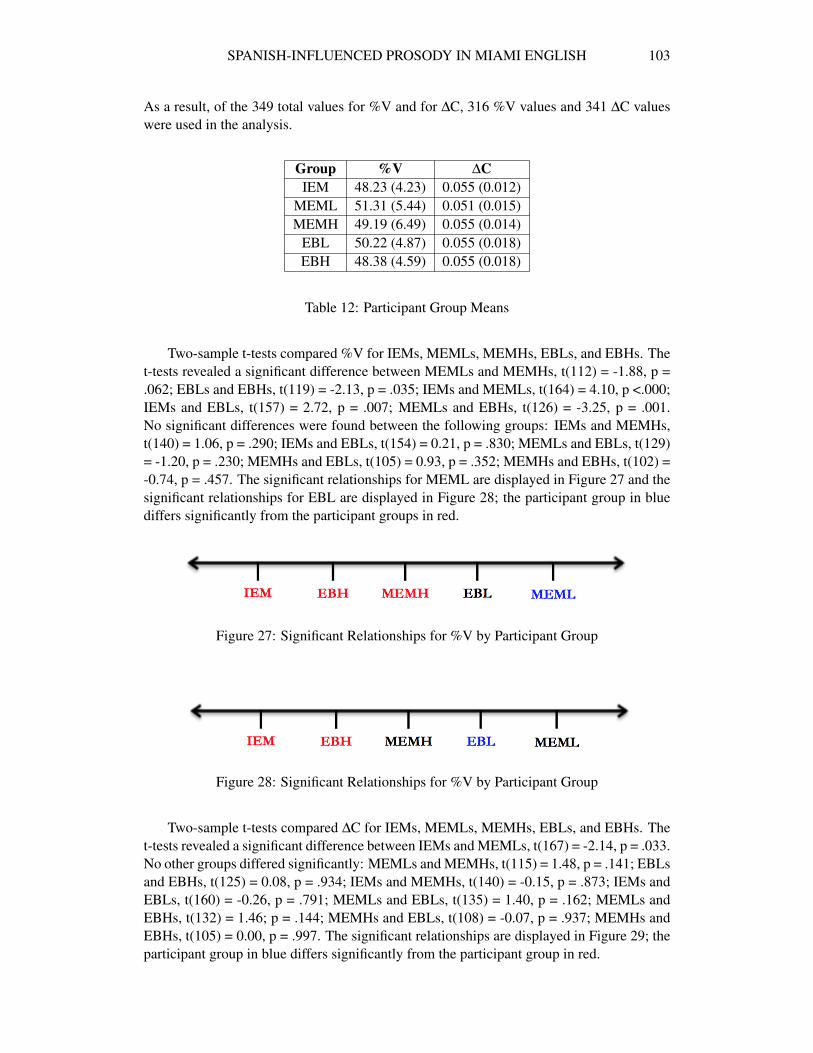
Two-sample t-tests compared %V for IEMs, MEMLs, MEMHs, EBLs, and EBHs. Thet-tests revealed a significant difference between MEMLs and MEMHs, t(112) = -1.88, p =.062; EBLs and EBHs, t(119) = -2.13, p = .035; IEMs and MEMLs, t(164) = 4.10, p <.000;IEMs and EBLs, t(157) = 2.72, p = .007; MEMLs and EBHs, t(126) = -3.25, p = .001.No significant differences were found between the following groups: IEMs and MEMHs,t(140) = 1.06, p = .290; IEMs and EBLs, t(154) = 0.21, p = .830; MEMLs and EBLs, t(129)= -1.20, p = .230; MEMHs and EBLs, t(105) = 0.93, p = .352; MEMHs and EBHs, t(102) =-0.74, p = .457. The significant relationships for MEML are displayed in Figure 27 and thesignificant relationships for EBL are displayed in Figure 28; the participant group in bluediffers significantly from the participant groups in red.



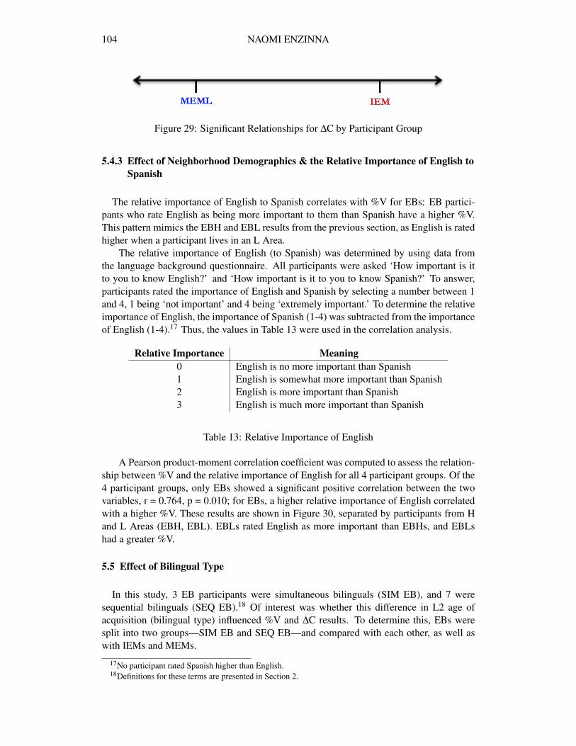
Two-sample t-tests compared ∆C for IEMs, MEMLs, MEMHs, EBLs, and EBHs. Thet-tests revealed a significant difference between IEMs and MEMLs, t(167) = -2.14, p = .033.No other groups differed significantly: MEMLs and MEMHs, t(115) = 1.48, p = .141; EBLsand EBHs, t(125) = 0.08, p = .934; IEMs and MEMHs, t(140) = -0.15, p = .873; IEMs andEBLs, t(160) = -0.26, p = .791; MEMLs and EBLs, t(135) = 1.40, p = .162; MEMLs andEBHs, t(132) = 1.46; p = .144; MEMHs and EBLs, t(108) = -0.07, p = .937; MEMHs andEBHs, t(105) = 0.00, p = .997. The significant relationships are displayed in Figure 29; theparticipant group in blue differs significantly from the participant group in red.

104 NAOMI ENZINNA

Figure 29: Significant Relationships for ∆C by Participant Group

5.4.3 Effect of Neighborhood Demographics & the Relative Importance of English toSpanish

The relative importance of English to Spanish correlates with %V for EBs: EB partici-pants who rate English as being more important to them than Spanish have a higher %V.This pattern mimics the EBH and EBL results from the previous section, as English is ratedhigher when a participant lives in an L Area.

The relative importance of English (to Spanish) was determined by using data fromthe language background questionnaire. All participants were asked ‘How important is itto you to know English?’ and ‘How important is it to you to know Spanish?’ To answer,participants rated the importance of English and Spanish by selecting a number between 1and 4, 1 being ‘not important’ and 4 being ‘extremely important.’ To determine the relativeimportance of English, the importance of Spanish (1-4) was subtracted from the importanceof English (1-4).17 Thus, the values in Table 13 were used in the correlation analysis.

Relative Importance Meaning0 English is no more important than Spanish1 English is somewhat more important than Spanish2 English is more important than Spanish3 English is much more important than Spanish

Table 13: Relative Importance of English

A Pearson product-moment correlation coefficient was computed to assess the relation-ship between %V and the relative importance of English for all 4 participant groups. Of the4 participant groups, only EBs showed a significant positive correlation between the twovariables, r = 0.764, p = 0.010; for EBs, a higher relative importance of English correlatedwith a higher %V. These results are shown in Figure 30, separated by participants from Hand L Areas (EBH, EBL). EBLs rated English as more important than EBHs, and EBLshad a greater %V.

5.5 Effect of Bilingual Type

In this study, 3 EB participants were simultaneous bilinguals (SIM EB), and 7 weresequential bilinguals (SEQ EB).18 Of interest was whether this difference in L2 age ofacquisition (bilingual type) influenced %V and ∆C results. To determine this, EBs weresplit into two groups—SIM EB and SEQ EB—and compared with each other, as well aswith IEMs and MEMs.

17No participant rated Spanish higher than English.18Definitions for these terms are presented in Section 2.


Figure 30: Correlation of %V and Relative Importance of English for EBs

The by-subject results (Section 5.5.1) suggest that bilingual type does not influence%V or ∆C. The by-utterance results (Section 5.5.2) show that SIM EBs have a significantlygreater %V than IEMs, but SEQ EBs do not.

5.5.1 Effect of Bilingual Type by Subject

The mean %V and ∆C for each participant group are shown in Table 14. For results in thissection, all data two standard deviations from the mean were removed from the analysis.As a result, one MEM participant’s %V (57.09). No EBs were excluded.

Group %V ∆CIEM 47.65 (1.18) 0.057 (0.005)

MEM 49.91 (1.87) 0.056 (0.005)SIM EB 49.40 (1.49) 0.059 (0.005)SEQ EB 49.68 (1.42) 0.057 (0.008)


Two-sample t-tests compared %V for IEMs, MEMs, SIM EBs, and SEQ EBs. The t-tests revealed a significant difference between IEMs and SIM EBs, t(11) = -2.12, p = .055;IEMs and SEQ EBs, t(15) = 3.21, p = .005; and IEMs and MEMs, t(17) = -3.17, p = .005.No other comparison was significant: SIM EBs and SEQ EBs, t(8) = 0.28, p = .786; MEMsand SIM EBs, t(10) = 0.41, p = .684; MEMs and SEQ EBs, t(14) = -0.26, p = .796. Thesignificant relationships are displayed in Figure 31; the participant group in blue differssignificantly the participant groups in red.

106 NAOMI ENZINNA


Two-sample t-tests compared ∆C for IEMs, MEMs, SIM EBs, and SEQ EBs. The t-tests did not reveal a significant difference between groups: SIM EBs and SEQ EBs, t(8) =-0.31, p = .758; IEMs and SIM EBs, t(11) = -0.52, p = .606; IEMs and SEQ EBs, t(15) =0.07, p = .940; MEMs and SIM EBs, t(11) = 0.00, p = .545; MEMs and SEQ EBs, t(15) =0.20, p = .841.

5.5.2 Effect of Bilingual Type by Utterance


Group %V ∆CIEM 47.65 (1.18) 0.057 (0.005)

MEM 49.91 (1.87) 0.056 (0.005)SIM EB 49.94 (4.63) 0.056 (0.018)SEQ EB 49.01 (4.89) 0.054 (0.018)


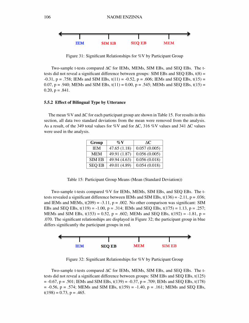
Two-sample t-tests compared %V for IEMs, MEMs, SIM EBs, and SEQ EBs. The t-tests revealed a significant difference between IEMs and SIM EBs, t(136) = -2.11, p = .036;and IEMs and MEMs, t(209) = -3.11, p = .002. No other comparison was significant: SIMEBs and SEQ EBs, t(119) = -1.00, p = .314; IEMs and SEQ EBs, t(175) = 1.13, p = .257;MEMs and SIM EBs, t(153) = 0.52, p = .602; MEMs and SEQ EBs, t(192) = -1.81, p =.070. The significant relationships are displayed in Figure 32; the participant group in bluediffers significantly the participant groups in red.


Two-sample t-tests compared ∆C for IEMs, MEMs, SIM EBs, and SEQ EBs. The t-tests did not reveal a significant difference between groups: SIM EBs and SEQ EBs, t(125)= -0.67, p = .501; IEMs and SIM EBs, t(139) = -0.37, p = .709; IEMs and SEQ EBs, t(178)= -0.56, p = .574; MEMs and SIM EBs, t(159) = -1.40, p = .161; MEMs and SEQ EBs,t(198) = 0.73, p = .465.


5.6 Late Bilingual L2 Difficulty

Several results from this study suggest that LB participants have difficulty producing (orreading in) their L2.

First, as reported in section 5.2, LBs have a significantly lower %V than MEMs. Thisresult is unexpected because Spanish has a higher %V than English (Ramus et al., 1999).To account for this difference, the duration of two consonant clusters (‘str’ in ‘strikes’and ‘ndr’ in ’raindrops’) and two reduced vowels (the first ‘a’ in ‘apparently’ and ‘i’ in‘beautiful’)19 were measured in the speech of all 40 participants. The results show that LBshave the greatest mean duration of consonant clusters; this suggests that LBs have difficultyproducing consonant clusters, increasing %C and lowering %V as a result. Second, theresults show that LBs have the greatest mean duration of (what is expected to be) reducedvowels. This finding supports the claim that L2 learners of English have difficulty acquiringand producing English stress patterns (Nava, 2011). The mean durations (in seconds) arepresented in the Table 16.

ALL IEM MEM EB LBConsonant Cluster 0.132 0.125 0.125 0.124 0.155Reduced Vowel 0.089 0.081 0.086 0.080 0.110

Table 16: Mean Durations (s) of Random Clusters and Reduced Vowels

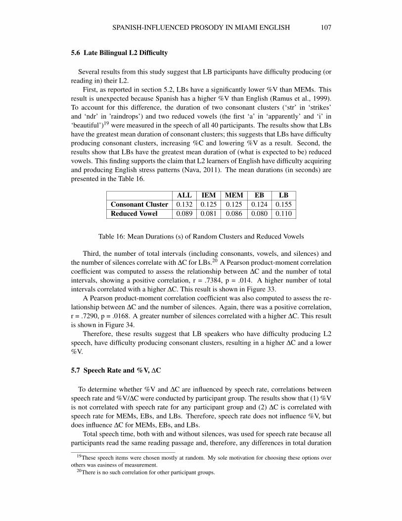
Third, the number of total intervals (including consonants, vowels, and silences) andthe number of silences correlate with ∆C for LBs.20 A Pearson product-moment correlationcoefficient was computed to assess the relationship between ∆C and the number of totalintervals, showing a positive correlation, r = .7384, p = .014. A higher number of totalintervals correlated with a higher ∆C. This result is shown in Figure 33.

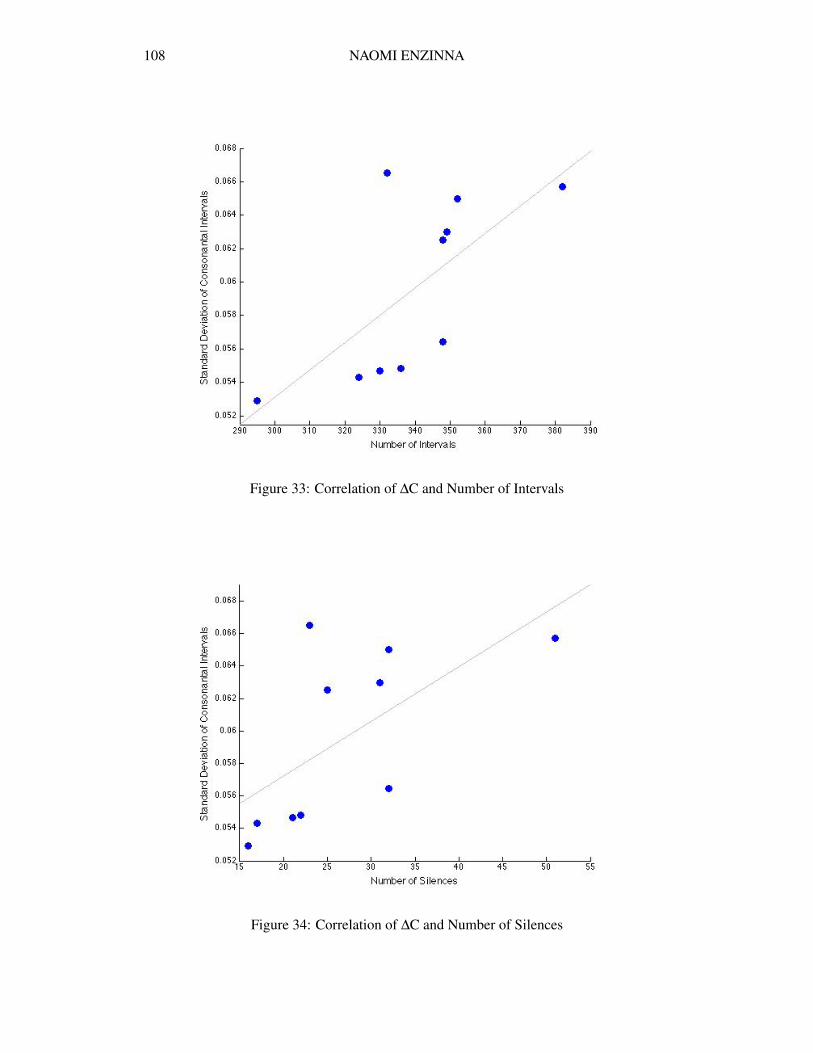
A Pearson product-moment correlation coefficient was also computed to assess the re-lationship between ∆C and the number of silences. Again, there was a positive correlation,r = .7290, p = .0168. A greater number of silences correlated with a higher ∆C. This resultis shown in Figure 34.

Therefore, these results suggest that LB speakers who have difficulty producing L2speech, have difficulty producing consonant clusters, resulting in a higher ∆C and a lower%V.

5.7 Speech Rate and %V, ∆C

To determine whether %V and ∆C are influenced by speech rate, correlations betweenspeech rate and %V/∆C were conducted by participant group. The results show that (1) %Vis not correlated with speech rate for any participant group and (2) ∆C is correlated withspeech rate for MEMs, EBs, and LBs. Therefore, speech rate does not influence %V, butdoes influence ∆C for MEMs, EBs, and LBs.

Total speech time, both with and without silences, was used for speech rate because allparticipants read the same reading passage and, therefore, any differences in total duration

19These speech items were chosen mostly at random. My sole motivation for choosing these options overothers was easiness of measurement.

20There is no such correlation for other participant groups.

108 NAOMI ENZINNA

Figure 33: Correlation of ∆C and Number of Intervals

Figure 34: Correlation of ∆C and Number of Silences


time would depend on how fast or slow the participant read. Both the total duration withand without silences produced the same significant correlations.

5.7.1 Speech Rate and %V

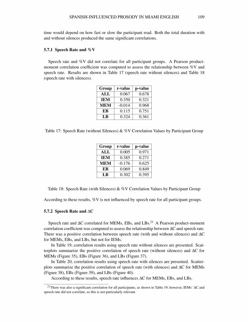
Speech rate and %V did not correlate for all participant groups. A Pearson product-moment correlation coefficient was computed to assess the relationship between %V andspeech rate. Results are shown in Table 17 (speech rate without silences) and Table 18(speech rate with silences).

Group r-value p-valueALL 0.067 0.678IEM 0.350 0.321

MEM -0.014 0.968EB 0.115 0.751LB 0.324 0.361

Table 17: Speech Rate (without Silences) & %V Correlation Values by Participant Group

Group r-value p-valueALL 0.005 0.971IEM 0.385 0.271

MEM -0.176 0.625EB 0.069 0.849LB 0.302 0.395

Table 18: Speech Rate (with Silences) & %V Correlation Values by Participant Group

According to these results, %V is not influenced by speech rate for all participant groups.

5.7.2 Speech Rate and ∆C

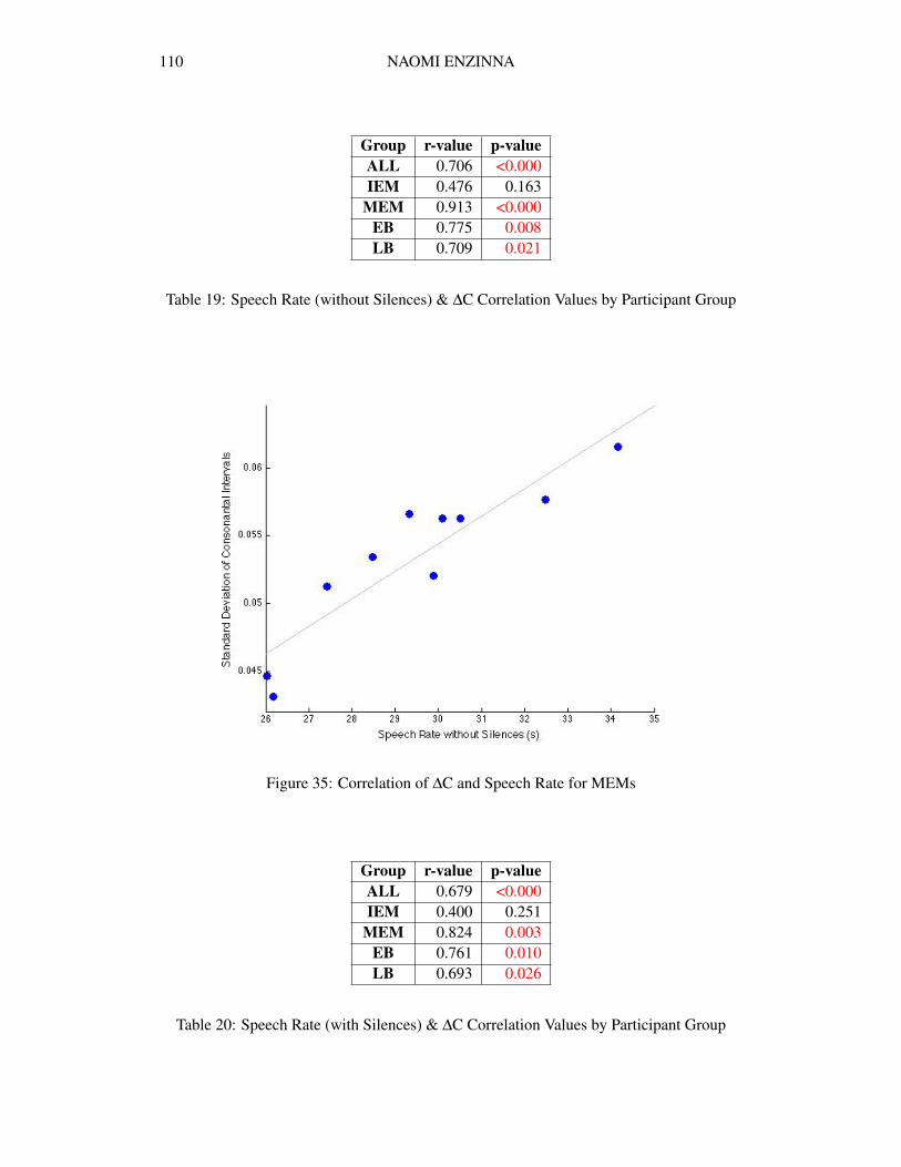
Speech rate and ∆C correlated for MEMs, EBs, and LBs.21 A Pearson product-momentcorrelation coefficient was computed to assess the relationship between ∆C and speech rate.There was a positive correlation between speech rate (with and without silences) and ∆Cfor MEMs, EBs, and LBs, but not for IEMs.

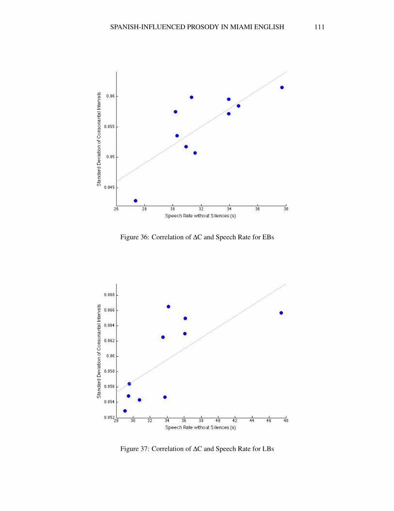
In Table 19, correlation results using speech rate without silences are presented. Scat-terplots summarize the positive correlation of speech rate (without silences) and ∆C forMEMs (Figure 35), EBs (Figure 36), and LBs (Figure 37).

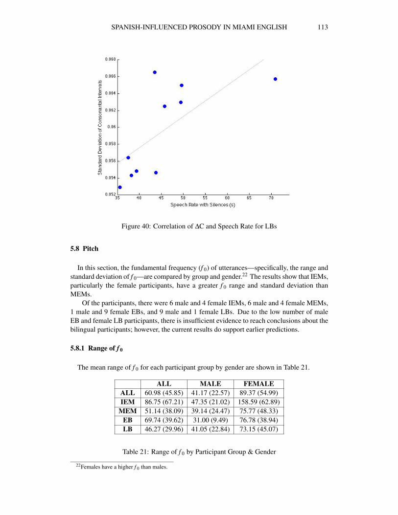
In Table 20, correlation results using speech rate with silences are presented. Scatter-plots summarize the positive correlation of speech rate (with silences) and ∆C for MEMs(Figure 38), EBs (Figure 39), and LBs (Figure 40).

According to these results, speech rate influences ∆C for MEMs, EBs, and LBs.

21There was also a significant correlation for all participants, as shown in Table 19; however, IEMs’ ∆C andspeech rate did not correlate, so this is not particularly relevant.

110 NAOMI ENZINNA

Group r-value p-valueALL 0.706 <0.000IEM 0.476 0.163

MEM 0.913 <0.000EB 0.775 0.008LB 0.709 0.021

Table 19: Speech Rate (without Silences) & ∆C Correlation Values by Participant Group

Figure 35: Correlation of ∆C and Speech Rate for MEMs

Group r-value p-valueALL 0.679 <0.000IEM 0.400 0.251

MEM 0.824 0.003EB 0.761 0.010LB 0.693 0.026

Table 20: Speech Rate (with Silences) & ∆C Correlation Values by Participant Group


Figure 36: Correlation of ∆C and Speech Rate for EBs

Figure 37: Correlation of ∆C and Speech Rate for LBs

112 NAOMI ENZINNA

Figure 38: Correlation of ∆C and Speech Rate for MEMs

Figure 39: Correlation of ∆C and Speech Rate for EBs


Figure 40: Correlation of ∆C and Speech Rate for LBs

5.8 Pitch

In this section, the fundamental frequency (f 0) of utterances—specifically, the range andstandard deviation of f 0—are compared by group and gender.22 The results show that IEMs,particularly the female participants, have a greater f 0 range and standard deviation thanMEMs.

Of the participants, there were 6 male and 4 female IEMs, 6 male and 4 female MEMs,1 male and 9 female EBs, and 9 male and 1 female LBs. Due to the low number of maleEB and female LB participants, there is insufficient evidence to reach conclusions about thebilingual participants; however, the current results do support earlier predictions.

5.8.1 Range of f 0

The mean range of f 0 for each participant group by gender are shown in Table 21.

ALL MALE FEMALEALL 60.98 (45.85) 41.17 (22.57) 89.37 (54.99)IEM 86.75 (67.21) 47.35 (21.02) 158.59 (62.89)

MEM 51.14 (38.09) 39.14 (24.47) 75.77 (48.33)EB 69.74 (39.62) 31.00 (9.49) 76.78 (38.94)LB 46.27 (29.96) 41.05 (22.84) 73.15 (45.07)

Table 21: Range of f 0 by Participant Group & Gender

22Females have a higher f 0 than males.

114 NAOMI ENZINNA

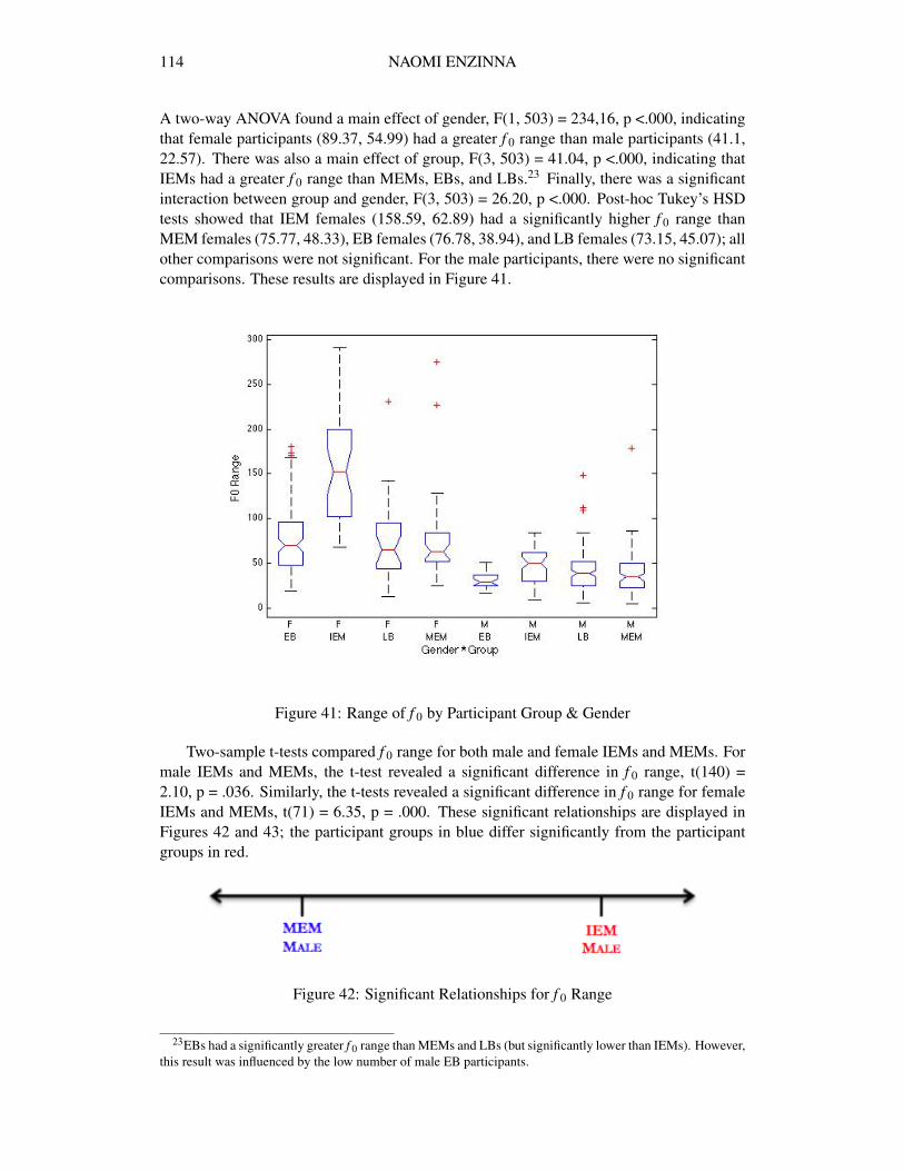
A two-way ANOVA found a main effect of gender, F(1, 503) = 234,16, p <.000, indicatingthat female participants (89.37, 54.99) had a greater f 0 range than male participants (41.1,22.57). There was also a main effect of group, F(3, 503) = 41.04, p <.000, indicating thatIEMs had a greater f 0 range than MEMs, EBs, and LBs.23 Finally, there was a significantinteraction between group and gender, F(3, 503) = 26.20, p <.000. Post-hoc Tukey’s HSDtests showed that IEM females (158.59, 62.89) had a significantly higher f 0 range thanMEM females (75.77, 48.33), EB females (76.78, 38.94), and LB females (73.15, 45.07); allother comparisons were not significant. For the male participants, there were no significantcomparisons. These results are displayed in Figure 41.

Figure 41: Range of f 0 by Participant Group & Gender

Two-sample t-tests compared f 0 range for both male and female IEMs and MEMs. Formale IEMs and MEMs, the t-test revealed a significant difference in f 0 range, t(140) =2.10, p = .036. Similarly, the t-tests revealed a significant difference in f 0 range for femaleIEMs and MEMs, t(71) = 6.35, p = .000. These significant relationships are displayed inFigures 42 and 43; the participant groups in blue differ significantly from the participantgroups in red.

Figure 42: Significant Relationships for f 0 Range

23EBs had a significantly greater f 0 range than MEMs and LBs (but significantly lower than IEMs). However,this result was influenced by the low number of male EB participants.


Figure 43: Significant Relationships for f 0 Range

5.8.2 Standard Deviation of f 0

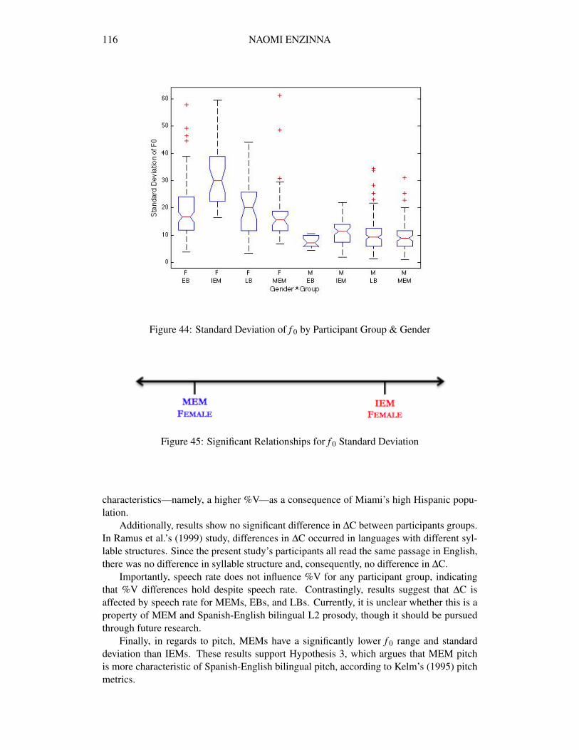
The mean standard deviation of f 0 for each participant group by gender is shown inTable 22.

ALL MALE FEMALEALL 14.48 (10.12) 9.87 (5.26) 21.10 (11.64)IEM 18.45 (13.32) 10.57 (4.80) 32.82 (11.78)

MEM 12.11 (8.17) 9.51 (5.13) 17.45 (10.43)EB 17.30 (10.30) 7.54 (2.17) 19.07 (10.21)LB 11.69 (7.51) 10.10 (5.76) 19.86 (9.97)

Table 22: Standard Deviation of f 0 by Participant Group & Gender (Mean (Std. Dev.))

A two-way ANOVA found a main effect of gender, F(1, 503) = 231.14, p <.000, indicat-ing that the standard deviation of f 0 was greater for female participants (21.10, 11.64) thanmale participants (9.87, 5.26). There was also a main effect of group, F(3, 503) = 22.27, p<.000.24 Finally, there was a significant interaction between group and gender, F(3, 503) =15.30, p <.000. Post-hoc Tukey’s HSD tests showed there were no significant differencesin the standard deviation of f 0 for male participants. For the female participants, how-ever, IEMs (32.82, 11.78) had a significantly higher standard deviation of f 0 than MEMs(17.45, 10.43), EBs (19.07, 10.21), LBs (19.86, 9.97); no other comparisons were signifi-cant. These results are displayed in Figure 44.

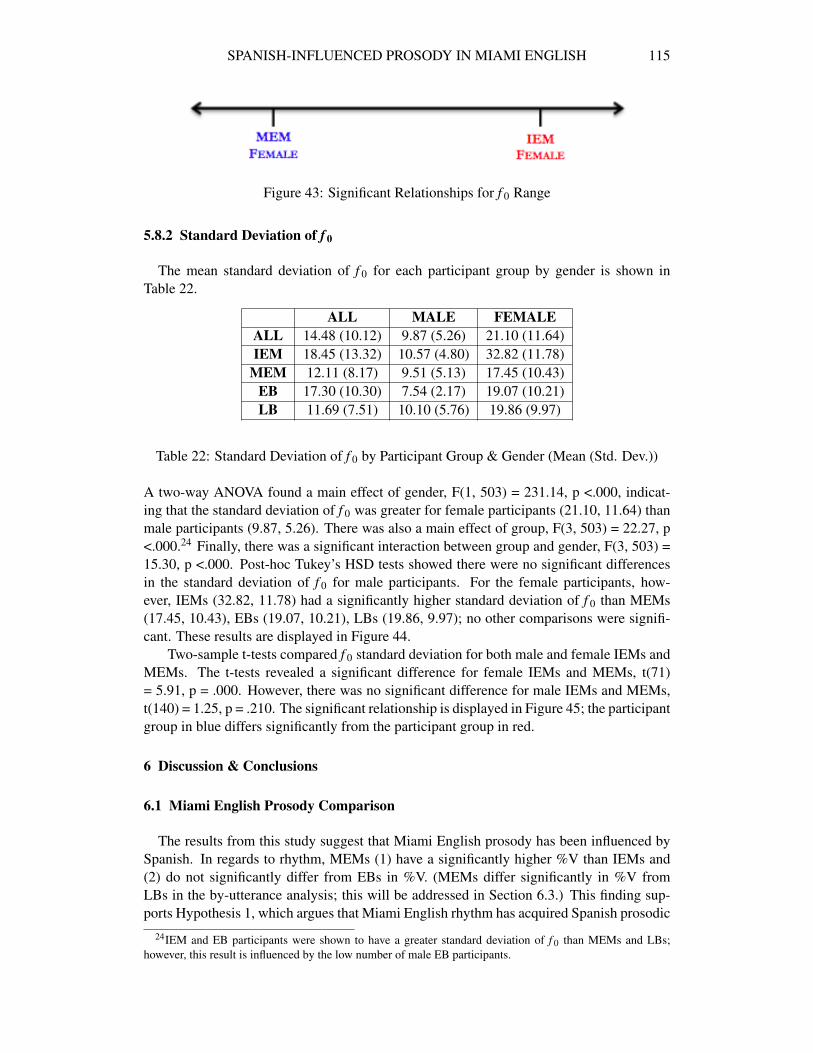
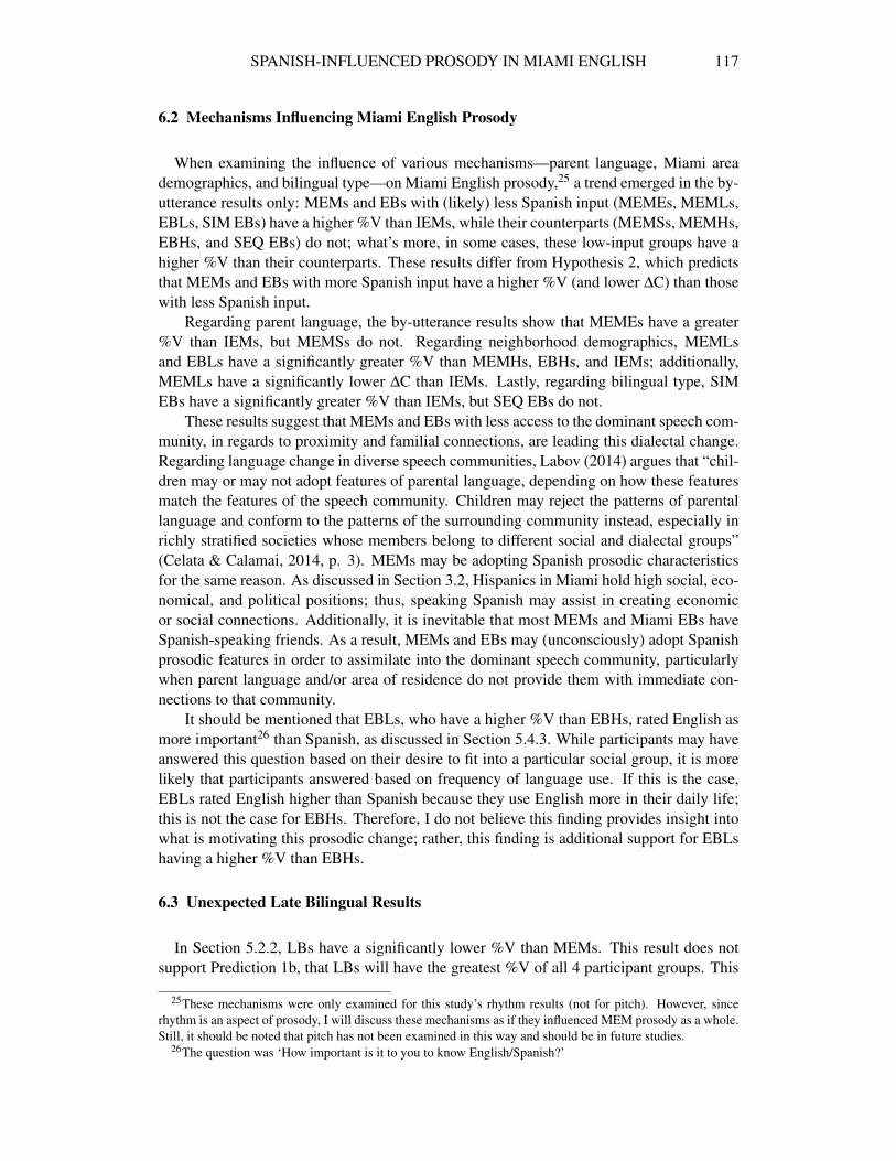
Two-sample t-tests compared f 0 standard deviation for both male and female IEMs andMEMs. The t-tests revealed a significant difference for female IEMs and MEMs, t(71)= 5.91, p = .000. However, there was no significant difference for male IEMs and MEMs,t(140) = 1.25, p = .210. The significant relationship is displayed in Figure 45; the participantgroup in blue differs significantly from the participant group in red.

6 Discussion & Conclusions

6.1 Miami English Prosody Comparison

The results from this study suggest that Miami English prosody has been influenced bySpanish. In regards to rhythm, MEMs (1) have a significantly higher %V than IEMs and(2) do not significantly differ from EBs in %V. (MEMs differ significantly in %V fromLBs in the by-utterance analysis; this will be addressed in Section 6.3.) This finding sup-ports Hypothesis 1, which argues that Miami English rhythm has acquired Spanish prosodic

24IEM and EB participants were shown to have a greater standard deviation of f 0 than MEMs and LBs;however, this result is influenced by the low number of male EB participants.

116 NAOMI ENZINNA

Figure 44: Standard Deviation of f 0 by Participant Group & Gender

Figure 45: Significant Relationships for f 0 Standard Deviation

characteristics—namely, a higher %V—as a consequence of Miami’s high Hispanic popu-lation.

Additionally, results show no significant difference in ∆C between participants groups.In Ramus et al.’s (1999) study, differences in ∆C occurred in languages with different syl-lable structures. Since the present study’s participants all read the same passage in English,there was no difference in syllable structure and, consequently, no difference in ∆C.

Importantly, speech rate does not influence %V for any participant group, indicatingthat %V differences hold despite speech rate. Contrastingly, results suggest that ∆C isaffected by speech rate for MEMs, EBs, and LBs. Currently, it is unclear whether this is aproperty of MEM and Spanish-English bilingual L2 prosody, though it should be pursuedthrough future research.

Finally, in regards to pitch, MEMs have a significantly lower f 0 range and standarddeviation than IEMs. These results support Hypothesis 3, which argues that MEM pitchis more characteristic of Spanish-English bilingual pitch, according to Kelm’s (1995) pitchmetrics.


6.2 Mechanisms Influencing Miami English Prosody

When examining the influence of various mechanisms—parent language, Miami areademographics, and bilingual type—on Miami English prosody,25 a trend emerged in the by-utterance results only: MEMs and EBs with (likely) less Spanish input (MEMEs, MEMLs,EBLs, SIM EBs) have a higher %V than IEMs, while their counterparts (MEMSs, MEMHs,EBHs, and SEQ EBs) do not; what’s more, in some cases, these low-input groups have ahigher %V than their counterparts. These results differ from Hypothesis 2, which predictsthat MEMs and EBs with more Spanish input have a higher %V (and lower ∆C) than thosewith less Spanish input.

Regarding parent language, the by-utterance results show that MEMEs have a greater%V than IEMs, but MEMSs do not. Regarding neighborhood demographics, MEMLsand EBLs have a significantly greater %V than MEMHs, EBHs, and IEMs; additionally,MEMLs have a significantly lower ∆C than IEMs. Lastly, regarding bilingual type, SIMEBs have a significantly greater %V than IEMs, but SEQ EBs do not.

These results suggest that MEMs and EBs with less access to the dominant speech com-munity, in regards to proximity and familial connections, are leading this dialectal change.Regarding language change in diverse speech communities, Labov (2014) argues that “chil-dren may or may not adopt features of parental language, depending on how these featuresmatch the features of the speech community. Children may reject the patterns of parentallanguage and conform to the patterns of the surrounding community instead, especially inrichly stratified societies whose members belong to different social and dialectal groups”(Celata & Calamai, 2014, p. 3). MEMs may be adopting Spanish prosodic characteristicsfor the same reason. As discussed in Section 3.2, Hispanics in Miami hold high social, eco-nomical, and political positions; thus, speaking Spanish may assist in creating economicor social connections. Additionally, it is inevitable that most MEMs and Miami EBs haveSpanish-speaking friends. As a result, MEMs and EBs may (unconsciously) adopt Spanishprosodic features in order to assimilate into the dominant speech community, particularlywhen parent language and/or area of residence do not provide them with immediate con-nections to that community.

It should be mentioned that EBLs, who have a higher %V than EBHs, rated English asmore important26 than Spanish, as discussed in Section 5.4.3. While participants may haveanswered this question based on their desire to fit into a particular social group, it is morelikely that participants answered based on frequency of language use. If this is the case,EBLs rated English higher than Spanish because they use English more in their daily life;this is not the case for EBHs. Therefore, I do not believe this finding provides insight intowhat is motivating this prosodic change; rather, this finding is additional support for EBLshaving a higher %V than EBHs.

6.3 Unexpected Late Bilingual Results

In Section 5.2.2, LBs have a significantly lower %V than MEMs. This result does notsupport Prediction 1b, that LBs will have the greatest %V of all 4 participant groups. This

25These mechanisms were only examined for this study’s rhythm results (not for pitch). However, sincerhythm is an aspect of prosody, I will discuss these mechanisms as if they influenced MEM prosody as a whole.Still, it should be noted that pitch has not been examined in this way and should be in future studies.

26The question was ‘How important is it to you to know English/Spanish?’

118 NAOMI ENZINNA

prediction assumed that L1 prosodic features would carry over into the L2. However, sev-eral durational comparisons from this study suggest that LBs have difficulty reading and/orproducing L2 speech, likely causing these unexpected results.

For example, LBs have the greatest mean duration for all consonant duration compar-isons. Table 4 shows that LBs have the greatest mean duration of consonantal intervals andTable 16 suggests that LBs have the greatest mean duration of consonant clusters. Theseresults suggest that the LBs have difficulty producing L2 consonants/consonant clusters.

Additionally, as shown in Table 5, LBs have the greatest mean total silence durationand the greatest mean number of silences. As shown in Table 6, LBs have the greatest meanduration of all intervals. Further, LBs’ total number of intervals and total number of silencescorrelate with ∆C: a greater ∆C occurred with a higher number of intervals and silences. Allof these findings support the notion that LBs’ L2 speech is affected by L2 reading and/orproduction difficulties.

As shown in Stockmal, Markus, and Bond (2005), who examined the rhythm of Latvianwhen spoken by native speakers and proficient and non-proficient learners, L2 productionis affected by slower reading times: “Proficient [L2] learners read somewhat more slowly,while the non-proficient learners were the slowest as one would expect . . . ∆C decreasedwith increasing speaking rate but there was no tendency for %V to increase” (61). However,unlike Stockmal, Markus, and Bond, %V was affected by production/reading difficulties inthis study (Section 5.2.2).

6.4 Methodology Critique

Several considerations should be taken into account regarding this study’s methodology.First, the principal investigator is an MEM with English-speaking parents and is from anarea of Miami with a low Hispanic population. It may be the case that participants similarto or different from the principal investigator may have adjusted their speech to be more orless similar prosodically.

Regarding the recordings, the Miami data differed from the Ithaca data in how it wascollected. The Ithaca data was collected in a sound booth, while the Miami data was col-lected using a portable recorder in a quiet room (or the quietest room available). As aresult, there were differences in recording quality, and some Miami participants may havebeen distracted by their environment. Contrastingly, the Ithaca participants may have foundthe recording environment to be formal and, as a result, used a more formal register thanthe Miami participants. Ideally, all groups should have been recorded in a sound booth butwith efforts made to make recording as informal as possible.

Regarding participants, more careful selection of the participants could have balancedthe mechanism-related participant categories and the gender of participants in the bilingualgroups. This would have led to a fairer comparison of groups, especially in the pitch portionof this study. Last, using LBs to represent Spanish prosody was not effective; instead,(monolingual) Spanish speech should have been recorded and used as a comparison againstthe English monolingual and EB speech.

6.5 Future Research

The data from this study could be used for several future research projects. Expandingthis current project, the data could be reanalyzed using PVI rhythm metrics; this would en-sure that the conclusions reached by this study hold despite the metric used. Additionally,


the interview data could be used to compare prosody in natural speech between participantgroups; these results could be compared with the current study’s results to assess differencesMEM prosody in natural versus read speech. Last, expanding on the 2013 news organiza-tions’ claims about Miami English, examining vowel shading and L-palatalization wouldprovide further empirical evidence for (or against) such claims.

Expanding on the results found in this study, the study could be repeated in a citywith similar demographics. This would show whether other English varieties have beeninfluenced by Spanish (or other languages) in similar ways. Of interest is whether similarmechanisms would be responsible for the acquisition of any Spanish-influenced speechcharacteristics.

6.6 Conclusion

Results from this study suggest that Miami is developing its own variety of English,one with Spanish-influenced prosody, and MEMs with less Spanish input are driving thisdialectal change. Prosodic properties of this variety include a higher %V and a lower f 0range and standard deviation.

This finding support Labov’s (2014) claim that children may adopt features of the dom-inant speech community and reject features of their parental language when the speechcommunity is largely stratified. In this case, MEMs with English-speaking parents are re-jecting English %V and adopting Spanish %V. The results in this study further extend thisclaim to neighborhood demographics: a speaker will adopt features of the dominant speechcommunity when the speaker has less direct access to that community. In this case, Englishmonolinguals living in Miami—a city with a high Hispanic population—adopt features ofSpanish when they live in areas of Miami with a low Hispanic population.

References

Arvaniti, Amalia. 2012. The usefulness of metrics in the quantification of speech rhythm. Journalof Phonetics 40:351 – 373.

Brookes, Mike. 1997. Voicebox: Speech processing toolbox for MATLAB.http://www.ee.ic.ac.uk/hp/staff/dmb/voicebox/voicebox.

Celata, Chiara, and Silvia Calamai. 2014. Introduction: Sociophonetic perspectives on languagevariation. In Advances in Sociophonetics, ed. S. Celata, C. & Calamai, 1–14. Amsterdam: JohnBenjamins Publishing Company.

Escudero, Paola. 2011. Speech processing in bilingual and multilingual listeners: The interrelationbetween sound perception and word recognition. In Oxford Handbook of Laboratory Phonology,ed. A. Cohn, C. Fougeron, and M. K. Huffman, 407–417. New York: Oxford University Press.

Haggin, Patience. 2013a. English in the 305 has its own distinct Miami sound. The Miami Herald .

Haggin, Patience. 2013b. Why locals embrace that heavy “l” or not. WLRN .

Holt, Lori. 2011. How perceptual and cognitive constraints affect learning of speech categories.In Oxford Handbook of Laboratory Phonology, ed. A. Cohn, C. Fougeron, and M. K. Huffman,348–358. New York: Oxford University Press.

Joyner, James. 2008. Spanish Miami’s primary language. Outside the Beltway .

Kelm, Orlando R. 1995. Acoustic measurement of Spanish and English pitch contours: native andnon-native speakers. Hispanic Linguistics 6:435–448.

Labov, William. 2006. A sociolinguistic perspective on sociophonetic research. Journal of Phonetics34:500–515.

120 NAOMI ENZINNA

Labov, William. 2014. The sociophonetic orientation of the language learner. Advances in Socio-phonetics 15:17.

Lynch, Andrew. 2000. Spanish-speaking Miami in sociolinguistic perspective: Bilingualism, recon-tact, and language maintenance among the Cuban-origin population. Research on Spanish in theU.S. .

Nava, Emily. 2010. Connecting Phrasal and Rhythmic Events: Evidence from Second LanguageSpeech. ERIC.

Ramus, Franck. 2002. Acoustic correlates of linguistic rhythm: Perspectives. Proceedings of SpeechProsody 115–120.

Ramus, Franck, Marina Nespor, and Jacques Mehler. 1999. Correlates of linguistic rhythm in thespeech signal. Cognition 73:265–292.

Stockmal, Verna, Dace Markus, and Dzintra Bond. 2005. Measures of native and non-native rhythmin a quantity language. Language and Speech 48:55–63.

Talkin, David. 1995. A robust algorithm for pitch tracking (RAPT). Speech coding and synthesis495:518.

Thomas, Erik R., and Phillip M. Carter. 2006. Prosodic rhythm and African American english.English World-Wide 27:331–355.

Tilsen, Sam, and Keith Johnson. 2008. Low-frequency Fourier analysis of speech rhythm. TheJournal of the Acoustical Society of America 124:EL34–EL39.

United States Census Bureau. 2014. State & county quickfacts. Accessed: 2014-12-01.Watts, Gabriella. 2013. Miami accents: How ‘Miamah’ turned into a different sort of twang. WLRN

.

Naomi EnzinnaDepartment of LinguisticsCornell UniversityIthaca, NY [email protected]

Spanish-inﬂuenced prosody in Miami...

Documents

Transcript of Spanish-inﬂuenced prosody in Miami...