Copyright ⓒ The Korean Society for Aeronautical & Space SciencesReceived: April 28, 2012 Accepted: June 1, 2012

154 http://ijass.org pISSN: 2093-274x eISSN: 2093-2480

Review PaperInt’l J. of Aeronautical & Space Sci. 13(2), 154–169 (2012)DOI:10.5139/IJASS.2012.13.2.154

Spacecraft Guidance Algorithms for Asteroid Intercept and Rendezvous Missions

Matt Hawkins1, Yanning Guo2 and Bong Wie3 Iowa State University, Ames, IA 50011

Abstract

This paper presents a comprehensive review of spacecraft guidance algorithms for asteroid intercept and rendezvous missions.

Classical proportional navigation (PN) guidance is reviewed first, followed by pulsed PN guidance, augmented PN guidance,

predictive feedback guidance, Lambert guidance, and other guidance laws based on orbit perturbation theory. Optimal feedback

guidance laws satisfying various terminal constraints are also discussed. Finally, the zero-effort-velocity (ZEV) error, analogous

to the well-known zero-effort-miss (ZEM) distance, is introduced, leading to a generalized ZEM/ZEV guidance law. These

various feedback guidance laws can be easily applied to real asteroid intercept and rendezvous missions. However, differing

mission requirements and spacecraft capabilities will require continued research on terminal-phase guidance laws.

Key words: asteroid intercept, asteroid rendezvous, terminal-phase guidance, optimal guidance

1. Introduction

Acknowledgement of the threat to planet Earth from the

impact of an asteroid or comet has led to increased interest

in studying asteroid intercept and rendezvous missions. In

addition to responding to a threatening asteroid, scientific

missions to asteroids and other small bodies are of interest.

NASA’s Deep Space 1 and Deep Impact missions, and JAXA’s

Hayabusa mission are examples of flyby, intercept/impact, and

rendezvous, respectively. The differing mission requirements

and spacecraft capabilities will require continued study on

terminal-phase guidance laws.

This paper will review a number of different feedback

guidance laws, starting with simple laws to enable intercept,

then going through more sophisticated laws, including laws

with specified terminal conditions, and optimal feedback

guidance laws. Simulation results are shown, proving the

practical effectiveness of such feedback guidance laws.

Proportional navigation (PN) guidance is one of the

earliest known feedback guidance laws. Zarchan [1] describes

PN guidance, as well as a method of augmenting it when

acceleration characteristics of the target are known or can be

assumed. These feedback guidance laws can be implemented

with on-off thrusters using a simple Schmitt trigger or other

pulse-modulation devices as described in Wie [2]. Zarchan [1]

also describes predictive guidance for targets whose primary

acceleration is due to a gravitational field. This is based

on Lambert’s theorem. Linearized predictive guidance is

possible, based on the state-error transition matrix described

by Vallado [3].

Gil-Fernández et al. [4, 5] describe various terminal-phase

guidance laws of a kinetic impactor as applied to the European

Space Agency’s Don Quijote mission (now cancelled). This

work was continued in more detail by Hawkins et al. [6].

This is an Open Access article distributed under the terms of the Creative Com-mons Attribution Non-Commercial License (http://creativecommons.org/licenses/by-nc/3.0/) which permits unrestricted non-commercial use, distribution, and reproduc-tion in any medium, provided the original work is properly cited.

1Ph.D. Candidate 2 Visiting Student (2010 – 2012). Ph.D. Candidate, Department of Control Science

and Engineering, Harbin Institute of Technology, Harbin, People’s Republic of China 150001

3 Vance Coffman Endowed Chair Professor. Corresponding author. Email: bongwie@iastate.edu Tel: 1-515-294-3124 Fax: 1-515-294-3262.

20120430review.indd 154 2012-07-11 오후 1:50:17

155

Matt Hawkins Spacecraft Guidance Algorithms for Asteroid Intercept and Rendezvous Missions

http://ijass.org

Much work has been done on the problem of commanding

intercept at a specified impact angle. Some of the earliest

work led to guidance laws with strict limits on initial

conditions [7]. Since then, a number of different laws with

different advantages have been proposed. Various guidance

laws exist that do not require the time-to-go [8] that allow for

significant target maneuvers [9] and that can be used during

hypersonic flight [10]. Linear-quadratic control laws have

been derived in [11], and guidance laws based on classical

proportional navigation are described in [12]. Guidance laws

have been derived to follow a circular path to the target [13]

and to establish the desired end-of-mission geometry early

on [14]. Hawkins and Wie [15] investigated modified PN

guidance laws for asteroid intercept with terminal velocity

directional constraints.

Bryson and Ho [15] discussed optimal feedback control

laws for a simple rendezvous problem, considering both free-

terminal velocity and constrained-terminal velocity. They

also discussed the relationship between optimal feedback

control and proportional navigation guidance. Battin [16]

also discussed an optimal terminal-state vector control for

the orbit control problem, directly compensating for the

known disturbing gravitational acceleration. D’Souza [17]

further examined an optimal control algorithm in a uniform

gravitational field, and developed a computational method

to determine the optimal time-to-go.

Guo et al. [18] found three different optimal control laws

for certain constraints on terminal conditions. All three

laws require the terminal position to be specified, while the

terminal velocity can be fully specified, free, or constrained

along a particular direction. Hawkins et al. [19] compared

these guidance laws with PN-based guidance laws.

Ebrahimi et al. [20] proposed a robust optimal sliding

mode guidance law for an exoatmospheric interceptor, using

fixed-interval propulsive maneuvers. In this paper, gravity

was considered to be an explicit function of time. One major

contribution of Ebrahimi et al. was the new concept of the

zero-effort-velocity (ZEV) error, analogous to the well-known

zero-effort-miss (ZEM) distance. The ZEV is the velocity error

at the end of the mission if no further control accelerations

are imparted. Furfaro et al. [21] later employed the ZEM/

ZEV concept to construct two classes of non-linear guidance

algorithms for a lunar precision landing mission.

Guo et al. [22, 23] showed that in a uniform gravitational

field, the ZEM/ZEV logic is basically a generalized form of

various well-known optimal feedback guidance solutions

such as intercept or rendezvous, terminal guidance, and

planetary landing. A Mars landing example, originally

described by Acikmese and Ploen [24] is investigated in [23,

24]. In some cases ZEM/ZEV guidance can be improved by

introducing a number of waypoints. Details are given in [23,

24] on how to practically compute such waypoints in real

time. Finally, the ZEM/ZEV concept was also generalized to

other feedback guidance problems in [23, 24].

2. Mathematical modeling

The target asteroid can be modeled as a point mass in a

standard heliocentric Keplerian orbit, as follows:

(1)

where rT and vT are the position and velocity vectors of the

target and gT is the gravitational acceleration due to the sun,

expressed as

(2)

where is the solar gravitational parameter. Similarly,

the motion of the spacecraft is described by

(3)

where rS and vS are the position and velocity vectors of

the spacecraft, gS is again the gravitational acceleration

acting on the spacecraft due to the sun, and a is the control

acceleration provided by the spacecraft thrusters. In this

paper, a boldfaced symbol indicate a column matrix of a

physical vector expressed in a chosen inertial reference

frame.

In general, we have g = g(r, t). For some guidance

problems the gravitational acceleration can be considered

constant or negligible, but in general, the gravitational

acceleration must be considered a nonlinear function of

position. There are some other disturbing accelerations that

act on the spacecraft, such as solar radiation pressure and

the gravitational acceleration due to the asteroid. However,

intercept and rendezvous missions to small asteroids can

neglect these.

The relative position of the spacecraft with respect to the

target asteroid is then described by

(4)

The equation of motion of the spacecraft with respect to

the target becomes

(5)

20120430review.indd 155 2012-07-11 오후 1:50:18

DOI:10.5139/IJASS.2012.3.2.154 156

Int’l J. of Aeronautical & Space Sci. 3(2), 154–169 (2012)

where g represents the sum of apparent gravitational

accelerations on the target, as follows:

(6)

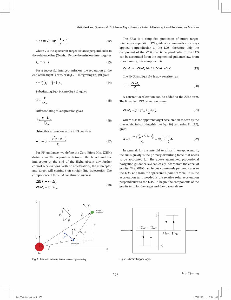
From Figure 1, it can be seen that

(7)

where λ is the line-of-sight (LOS) angle and (x, y) are the

components of the relative position vector along the inertial

(X, Y) coordinates. Differentiating this with respect to time

gives

(8)

where λ is the LOS rate and r = x 2+y 2. The rate of change

of the distance between the target and the spacecraft is the

closing velocity, found by differentiating r with respect to

time as

(9)

3. Guidance Laws

3.1 PN-based Feedback Guidance Laws

3.1.1 Classical Proportional Navigation (PN) Guidance

The first guidance law considered in this paper is the

so-called proportional navigation (PN) guidance. The PN

guidance attempts to drive the LOS rate to zero by applying

accelerations perpendicular to the LOS direction. The PN

guidance law is expressed as

(10)

where a is the acceleration command and n is the

effective navigation ratio, a designer-tunable parameter

[1]. The navigation ratio is typically chosen between 3 and

5. The optimal value, which will be derived and discussed

in a later section, is 3. Larger values are chosen to provide

more robustness against disturbances and errors. This can

be seen by inspecting Eq. (10). Inaccurate estimates of the

closing velocity or the LOS rate are equivalent to changing

the navigation ratio and using accurate closing velocity and

LOS rate information. Large navigation ratios will command

unnecessarily large accelerations, while small navigation

ratios risk commanding too little acceleration and missing

the target. Thus a larger navigation ratio ensures that

measurement errors will not make the accelerations too

small to achieve impact.

Because the acceleration commands are chosen to be

perpendicular to the LOS, the PN guidance law gives a scalar

value. The PN guidance acceleration command is then

expressed in the inertial reference frame as

(11)

The PN guidance law for steering an interceptor is also

called constant-bearing guidance, because it steers the

interceptor in such a way that the LOS does not rotate. An

interceptor using PN guidance, on a perfect collision course,

will maintain a constant bearing (i.e., λ is zero). When the

interceptor is not on a collision course, the trajectory is not

truly constant-bearing for n < ∞. As the effective navigation

ratio becomes very large, the LOS rate approaches zero faster,

at the expense of larger commanded acceleration.

The PN guidance law does not require the target or

interceptor velocities to be constant, nor does it require

the external accelerations to be zero. For small deviations

from constant velocity and small external accelerations, the

PN guidance law will still achieve intercept in a feedback

fashion. For the asteroid intercept scenario, the velocities

are approximately constant, and the external acceleration is

due almost entirely to the sun, and can be accounted for as

described below.

3.1.2 Augmented PN Guidance

The basic PN guidance law can overcome target accel-

erations in a feedback fashion. As can be seen from the

equations for LOS rate and closing velocity Vc, Eqs. (8) and (9),

the PN guidance law uses only the position and velocity of the

target, and is unable to take into account target accelerations

(if they exist). A guidance law which incorporates terms to

account for the target’s acceleration should be able to perform

better than the basic PN guidance law. Since the primary

target accelerations are from the sun’s gravity, the target’s

future accelerations are known. An augmented proportional

navigation guidance (APNG) law will now be discussed. As

with PNG, an easily tractable derivation will be given first,

and optimality will be considered in a later section.

From Figure 1, with a small-angle approximation, we

have

20120430review.indd 156 2012-07-11 오후 1:50:18

157

Matt Hawkins Spacecraft Guidance Algorithms for Asteroid Intercept and Rendezvous Missions

http://ijass.org

(12)

where y is the spacecraft-target distance perpendicular to

the reference line (X-axis). Define the mission time-to-go as

(13)

For a successful intercept mission, the separation at the

end of the flight is zero, or r(tf) = 0. Integrating Eq. (9) gives

(14)

Substituting Eq. (14) into Eq. (12) gives

(15)

Differentiating this expression gives

(16)

Using this expression in the PNG law gives

(17)

For PN guidance, we define the Zero-Effort-Miss (ZEM)

distance as the separation between the target and the

interceptor at the end of the flight, absent any further

control accelerations. With no accelerations, the interceptor

and target will continue on straight-line trajectories. The

components of the ZEM can thus be given as

(18)

The ZEM is a simplified prediction of future target-

interceptor separation. PN guidance commands are always

applied perpendicular to the LOS, therefore only the

component of the ZEM that is perpendicular to the LOS

can be accounted for in the augmented guidance law. From

trigonometry, this component is

(19)

The PNG law, Eq. (10), is now rewritten as

(20)

A constant acceleration can be added to the ZEM term.

The linearized ZEM equation is now

(21)

where aT is the apparent target acceleration as seen by the

spacecraft. Substituting this into Eq. (20), and using Eq. (17),

gives

(22)

In general, for the asteroid terminal intercept scenario,

the sun’s gravity is the primary disturbing force that needs

to be accounted for. The above augmented proportional

navigation guidance law can easily incorporate the effect of

gravity. The APNG law issues commands perpendicular to

the LOS, and from the spacecraft’s point of view. Thus the

acceleration term needed is the relative solar acceleration

perpendicular to the LOS. To begin, the components of the

gravity term for the target and the spacecraft are

43

Fig. 1. Asteroid intercept/rendezvous geometry.

Fig. 1. Asteroid intercept/rendezvous geometry.

44

UonUoff

- Uoff- Uon

1

-1

Fig. 2. Schmitt trigger logic.

Fig. 2. Schmitt trigger logic.

20120430review.indd 157 2012-07-11 오후 1:50:19

DOI:10.5139/IJASS.2012.3.2.154 158

Int’l J. of Aeronautical & Space Sci. 3(2), 154–169 (2012)

(23)

The components perpendicular to the LOS are

(24)

The target’s apparent acceleration perpendicular to the

LOS, as seen by the spacecraft, is

(25)

Substituting this equation into the APNG law, Eq. (22),

gives

(26)

In the inertial reference frame, the APNG law is expressed

as

(27)

As with PNG, the optimal navigation ratio for APNG is 3, to

be discussed in a later section.

3.1.3 Pulsed Guidance

For a simple intercept problem, the terminal velocity

is not specified, and is assumed to be the closing velocity

for PNG and APNG. The PNG and APNG laws assume that

continuously variable thrust is available. For thrusters with

no throttling ability, a different approach to guidance laws

is needed. Two approaches to formulating guidance laws

for fixed-thrust-level (on-off) guidance laws are PN-based

guidance laws and predictive guidance laws.

The PNG law continuously generates acceleration

commands to achieve intercept. Due to its feedback nature,

PNG will continue to generate guidance commands until

intercept is achieved. A special case of PNG occurs when

the interceptor is on a direct collision course. When this is

true, the guidance commands will be zero. When using PNG

logic, then, an acceleration command of zero means that the

interceptor is instantaneously on a direct collision course.

This fact can be exploited to use PNG logic for constant-

thrust engines.

Pulsed PNG (PPNG) logic computes the required

acceleration commands from PNG, but applies them in

continuous-thrust pulses. PPNG will “overshoot” the amount

of correction specified by PNG, until the PNG command is

zero. At that point, the interceptor is instantaneously on a

collision course, and the engines are turned off. If there were

no external accelerations or disturbances, the interceptor

would continue on an interception course. Because of the

acceleration due to the sun, this will not be the case, and a

further engine firing will be required later as the interceptor

“drifts” further and further from the straight-line collision

path.

Two approaches to determining when to fire engines

are threshold methods and timed methods. Both methods

will be described, as well as advantages and disadvantages

associated with each approach.

The threshold method can employ the so-called Schmitt

trigger or other pulse-modulation schemes [2]. Using a

Schmitt trigger, acceleration commands are calculated by

the PN guidance law as before. The trigger commands the

divert thrusters to turn on once the commanded acceleration

exceeds a certain magnitude, chosen by the designer, and

off when the commanded acceleration reaches a designer-

chosen cutoff. With traditional PN guidance the LOS rate

must reach zero for a successful intercept. Therefore the

second cutoff is typically selected as zero. The Schmitt trigger

control logic for pulsed proportional navigation guidance

(PPNG) is shown in Figure 2. The Schmitt trigger can also

be used for augmented PN guidance, giving an augmented

pulsed proportional navigation guidance (APPNG).

The timed method is similar to the threshold method in

that the PNG commands are still calculated, and applied

with constant thrust. As the name suggests, the difference

is that the timed method uses predetermined firing times

to turn on the thrusters. The designer must choose the firing

schedule. Typically at least three firings are required. An

early firing, near or at the beginning of the terminal mission

phase, is used to overcome most of the orbit injection errors.

The final firing comes shortly before impact, with enough

lead time to allow the thrust command to complete (e.g. the

commanded acceleration reaches zero), but close enough

to impact that only minimal further errors accumulate.

Additional intermediate firings provide robustness. As with

the Schmitt trigger, the timed method turns off thrusters

when the commanded thrust level is zero.

The advantage of these methods is the ability to use

constant-thrust on-off engines. The Schmitt trigger has

20120430review.indd 158 2012-07-11 오후 1:50:19

159

Matt Hawkins Spacecraft Guidance Algorithms for Asteroid Intercept and Rendezvous Missions

http://ijass.org

the same feedback advantages as PNG, in that it will issue

commands when the spacecraft is not on an intercept

course. A disadvantage of the Schmitt trigger is that the

designer must select the magnitude to turn on the thrusters.

Too small a magnitude risks excessive on-off cycles (chatter)

for the engines, while too large a magnitude risks missing the

target by failing to issue commands at all. An advantage of

the timed method is that the total number of on-off cycles

is known in advance and can be kept small. A disadvantage

is that the timed method might not issue commands even

when the calculated PNG commands are large.

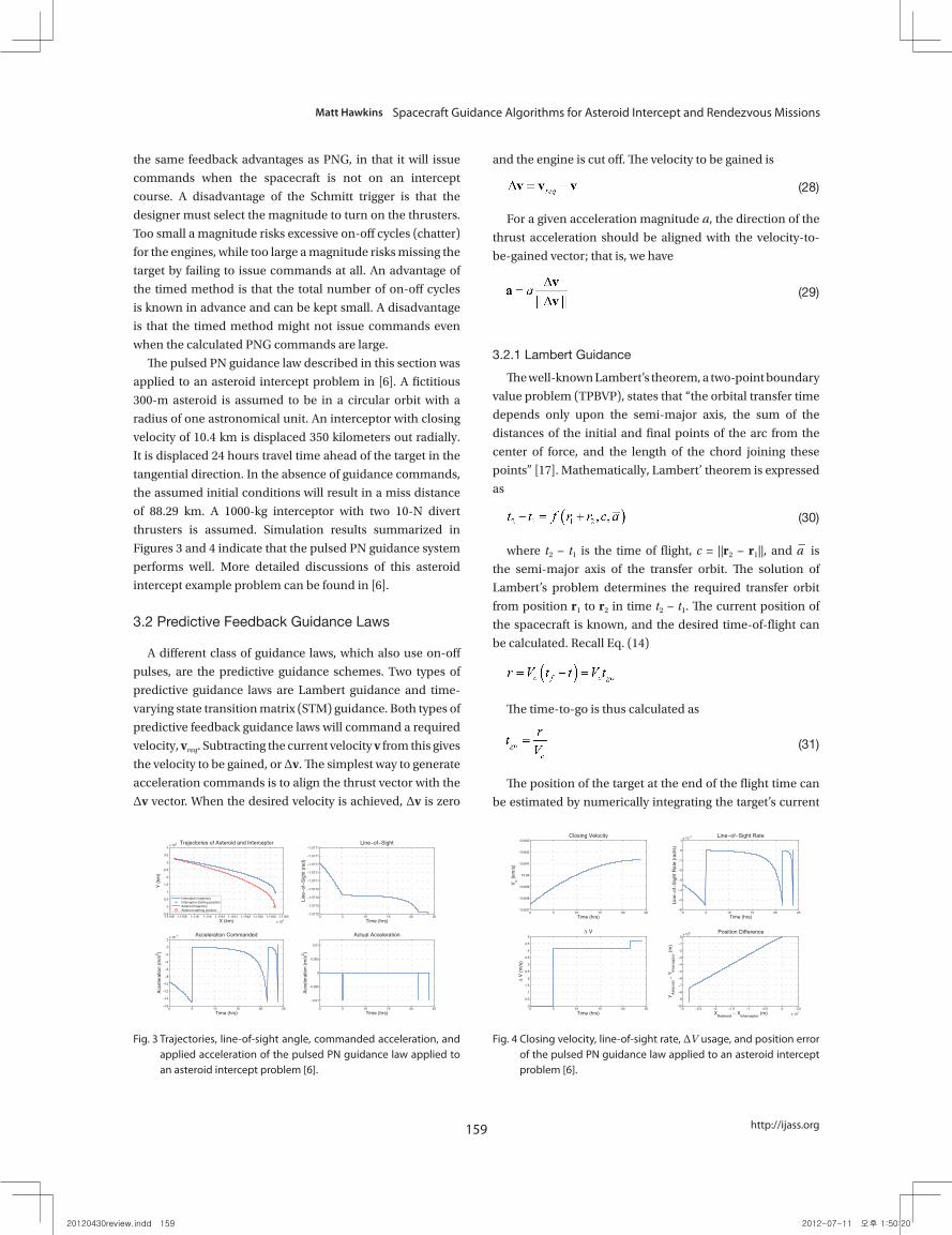
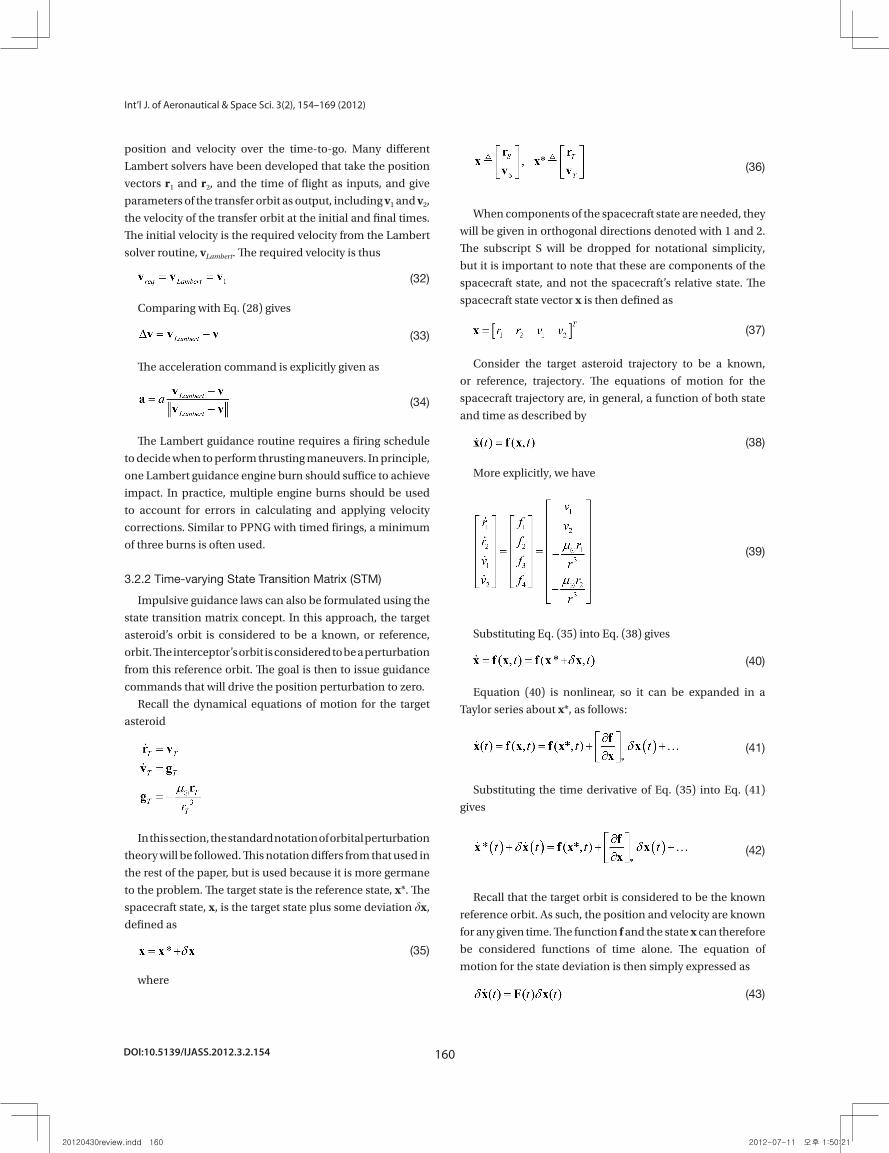
The pulsed PN guidance law described in this section was

applied to an asteroid intercept problem in [6]. A fictitious

300-m asteroid is assumed to be in a circular orbit with a

radius of one astronomical unit. An interceptor with closing

velocity of 10.4 km is displaced 350 kilometers out radially.

It is displaced 24 hours travel time ahead of the target in the

tangential direction. In the absence of guidance commands,

the assumed initial conditions will result in a miss distance

of 88.29 km. A 1000-kg interceptor with two 10-N divert

thrusters is assumed. Simulation results summarized in

Figures 3 and 4 indicate that the pulsed PN guidance system

performs well. More detailed discussions of this asteroid

intercept example problem can be found in [6].

3.2 Predictive Feedback Guidance Laws

A different class of guidance laws, which also use on-off

pulses, are the predictive guidance schemes. Two types of

predictive guidance laws are Lambert guidance and time-

varying state transition matrix (STM) guidance. Both types of

predictive feedback guidance laws will command a required

velocity, vreq. Subtracting the current velocity v from this gives

the velocity to be gained, or ∆v. The simplest way to generate

acceleration commands is to align the thrust vector with the

∆v vector. When the desired velocity is achieved, ∆v is zero

and the engine is cut off. The velocity to be gained is

(28)

For a given acceleration magnitude a, the direction of the

thrust acceleration should be aligned with the velocity-to-

be-gained vector; that is, we have

(29)

3.2.1 Lambert Guidance

The well-known Lambert’s theorem, a two-point boundary

value problem (TPBVP), states that “the orbital transfer time

depends only upon the semi-major axis, the sum of the

distances of the initial and final points of the arc from the

center of force, and the length of the chord joining these

points” [17]. Mathematically, Lambert’ theorem is expressed

as

(30)

where t2 − t1 is the time of flight, c = ||r2 − r1||, and a is

the semi-major axis of the transfer orbit. The solution of

Lambert’s problem determines the required transfer orbit

from position r1 to r2 in time t2 − t1. The current position of

the spacecraft is known, and the desired time-of-flight can

be calculated. Recall Eq. (14)

The time-to-go is thus calculated as

(31)

The position of the target at the end of the flight time can

be estimated by numerically integrating the target’s current

45

1.1159 1.1159 1.116 1.116 1.1161 1.1161 1.1162 1.1162 1.1163 1.1163

x 108

−0.5

0

0.5

1

1.5

2

2.5

3

3.5

4x 106 Trajectories of Asteroid and Interceptor

X (km)

Y (k

m)

Interceptor trajectoryInterceptor starting positionAsteroid trajectoryAsteroid starting position

0 5 10 15 20 25−1.5712

−1.5712

−1.5712

−1.5712

−1.5711

−1.5711

−1.5711

−1.5711

−1.5711Line−of−Sight

Time (hrs)

Line−o

f−S

ight

(rad

)

0 5 10 15 20 25−16

−14

−12

−10

−8

−6

−4

−2

0

2x 10−5 Acceleration Commanded

Time (hrs)

Acc

eler

atio

n (m

/s2 )

0 5 10 15 20 25

−0.01

−0.005

0

0.005

0.01

Actual Acceleration

Time (hrs)

Acc

eler

atio

n (m

/s2 )

Fig. 3 Trajectories, line-of-sight angle, commanded acceleration, and applied acceleration of the pulsed PN guidance law applied to an asteroid intercept problem [6].

Fig. 3 Trajectories, line-of-sight angle, commanded acceleration, and applied acceleration of the pulsed PN guidance law applied to an asteroid intercept problem [6].

46

0 5 10 15 20 2510.837

10.838

10.839

10.84

10.841

10.842

10.843Closing Velocity

Time (hrs)

Vc (k

m/s

)

0 5 10 15 20 25−6

−5

−4

−3

−2

−1

0

1x 10

−9 Line−of−Sight Rate

Time (hrs)

Line−o

f−S

ight

Rat

e (r

ad/s

)

0 5 10 15 20 250

0.5

1

1.5

2

2.5

3

3.5

4

4.5

5Δ V

Time (hrs)

Δ V

(m/s

)

−3 −2.5 −2 −1.5 −1 −0.5 0 0.5

x 105

−10

−9

−8

−7

−6

−5

−4

−3

−2

−1

0x 108 Position Difference

XAsteroid

− XInterceptor

(m)

YA

ster

oid −

YIn

terc

epto

r (m)

Fig. 4 Closing velocity, line-of-sight rate, VΔ usage, and position error of the pulsed PN guidance law applied to an asteroid intercept problem [6].

Fig. 4 Closing velocity, line-of-sight rate, ∆V usage, and position error of the pulsed PN guidance law applied to an asteroid intercept problem [6].

20120430review.indd 159 2012-07-11 오후 1:50:20

DOI:10.5139/IJASS.2012.3.2.154 160

Int’l J. of Aeronautical & Space Sci. 3(2), 154–169 (2012)

position and velocity over the time-to-go. Many different

Lambert solvers have been developed that take the position

vectors r1 and r2, and the time of flight as inputs, and give

parameters of the transfer orbit as output, including v1 and v2,

the velocity of the transfer orbit at the initial and final times.

The initial velocity is the required velocity from the Lambert

solver routine, vLambert. The required velocity is thus

(32)

Comparing with Eq. (28) gives

(33)

The acceleration command is explicitly given as

(34)

The Lambert guidance routine requires a firing schedule

to decide when to perform thrusting maneuvers. In principle,

one Lambert guidance engine burn should suffice to achieve

impact. In practice, multiple engine burns should be used

to account for errors in calculating and applying velocity

corrections. Similar to PPNG with timed firings, a minimum

of three burns is often used.

3.2.2 Time-varying State Transition Matrix (STM)

Impulsive guidance laws can also be formulated using the

state transition matrix concept. In this approach, the target

asteroid’s orbit is considered to be a known, or reference,

orbit. The interceptor’s orbit is considered to be a perturbation

from this reference orbit. The goal is then to issue guidance

commands that will drive the position perturbation to zero.

Recall the dynamical equations of motion for the target

asteroid

In this section, the standard notation of orbital perturbation

theory will be followed. This notation differs from that used in

the rest of the paper, but is used because it is more germane

to the problem. The target state is the reference state, x*. The

spacecraft state, x, is the target state plus some deviation δx,

defined as

(35)

where

(36)

When components of the spacecraft state are needed, they

will be given in orthogonal directions denoted with 1 and 2.

The subscript S will be dropped for notational simplicity,

but it is important to note that these are components of the

spacecraft state, and not the spacecraft’s relative state. The

spacecraft state vector x is then defined as

(37)

Consider the target asteroid trajectory to be a known,

or reference, trajectory. The equations of motion for the

spacecraft trajectory are, in general, a function of both state

and time as described by

(38)

More explicitly, we have

(39)

Substituting Eq. (35) into Eq. (38) gives

(40)

Equation (40) is nonlinear, so it can be expanded in a

Taylor series about x*, as follows:

(41)

Substituting the time derivative of Eq. (35) into Eq. (41)

gives

(42)

Recall that the target orbit is considered to be the known

reference orbit. As such, the position and velocity are known

for any given time. The function f and the state x can therefore

be considered functions of time alone. The equation of

motion for the state deviation is then simply expressed as

(43)

20120430review.indd 160 2012-07-11 오후 1:50:21

161

Matt Hawkins Spacecraft Guidance Algorithms for Asteroid Intercept and Rendezvous Missions

http://ijass.org

where F is the partial derivative term in Eq. (42), which is

the Jacobian of the function f evaluated at x* defined as

(44)

where is replaced with μ for notational simplicity.

Recall that the acceleration due to the sun’s gravity, Eq. (2),

is

The Jacobian of the gravitational force vector is often called

the gravity-gradient matrix defined as follows:

(45)

Observe that this corresponds to the bottom-left submatrix

of F, which can be written as a block matrix

(46)

where I and 0 are the identity matrix and the zero matrix of

conformal (in this case 2×2) size.

The general solution to Eq. (43) above can be expressed

as

(47)

where δx0 = δx(t0). Differentiating this gives

(48)

Substituting Eq. (48) into Eq. (43), and using Eq. (47), we

have

(49)

This must be true for any δx0, thus

(50)

with initial conditions given by

(51)

Equation (50) can be numerically integrated, starting with

the initial conditions given in Eq. (51), to find the current

estimate of the state transition matrix. However, for use in

generating a guidance law for asteroid intercept, it is desirable

to avoid numerical integration. As will be discussed in a later

section, if a numerical integration is to be performed, it is

better to simply integrate the equations of motion directly.

It is desirable to have an analytical expression of Φ for use in

guidance laws.

Consider the expression for the state error. Expanding this

into a Taylor series gives

(52)

Recalling Eq. (43), and taking its derivatives, gives

(53)

Comparing Eqs. (47) and (52) gives

(54)

Evaluating the expression in brackets gives the state-error

transition matrix as

(55)

This state-error transition matrix can be partitioned as

(56)

where

(57)

(58)

20120430review.indd 161 2012-07-11 오후 1:50:22

DOI:10.5139/IJASS.2012.3.2.154 162

Int’l J. of Aeronautical & Space Sci. 3(2), 154–169 (2012)

(59)

The simplest form of intercept guidance using the state-

error transition matrix uses only the position information

to generate a Δv command. The first-order approximation

for the final miss vector, absent any further acceleration

commands, is found as

(60)

The second term on the right-hand side is negligible for

small changes in closing velocity, giving

(61)

Consider driving the final relative position to zero. For

linearized dynamics, there are no external accelerations, so

we have

(62)

where vSTM is seen to be the velocity to be gained to ensure

impact.

For small changes in relative velocity, we have

(63)

The velocity change to be imparted becomes

(64)

The acceleration command vector is given, similar to

Lambert guidance, as

(65)

Using the gravity gradient matrix from Eq. (45), we can

show that

(66)

3.2.2.1 Predictive Impulsive Guidance

For practical implementation, we adopt the following

definitions

(67)

Substituting these into the guidance law in Eq. (64) gives

the predictive impulsive guidance law

(68)

3.2.2.2 Kinematic Impulsive Guidance

In terms of the line-of-sight angle, we have

(69)

The relative position can also be approximated as

(70)

and we obtain

(71)

The relative velocity can be approximated as a component

along the LOS and a component perpendicular to the LOS,

described as

(72)

Substituting Eq. (72) into Eq. (68) results in the kinematic

impulsive guidance law of the form

(73)

20120430review.indd 162 2012-07-11 오후 1:50:23

163

Matt Hawkins Spacecraft Guidance Algorithms for Asteroid Intercept and Rendezvous Missions

http://ijass.org

3.3 Optimal Feedback Guidance Algorithms

For some applications it is desirable to specify terminal

conditions on the interceptor. For intercept, the terminal

position is by definition zero. The terminal velocity, though,

may have direction or magnitude requirements, depending

on the mission. Optimal feedback guidance laws can be used

to achieve intercept, with the option of specifying the final

velocity.

Three different optimal feedback guidance laws are

considered for asteroid intercept and rendezvous missions.

The various forms of proportional navigation and predictive

guidance laws compute an estimated mission time-to-go

based on relative position and velocity. This computed

time-to-go is used as an input for the predictive laws, and

is available as an output of the proportional navigation

laws. In contrast, the optimal feedback guidance laws use a

specified time-to-go as a mission parameter, and compute

the acceleration commands needed to achieve intercept at

this pre-determined time.

When the final impact velocity vector (both impact velocity

and impact angle) is specified, the terminal velocity is

constrained. This leads to the constrained-terminal-velocity

guidance (CTVG) law. If the final velocity is free, the free-

terminal-velocity guidance (FTVG) law results, as discussed

in [18, 19]. When only the approach angle is commanded, the

velocity vector component along the desired final direction is

free, while the perpendicular components are constrained to

be zero. A combination of FTVG along the impact direction

and CTVG along the perpendicular directions allows

pointing of the final velocity vector, referred to as intercept-

angle-control guidance (IACG).

3.3.1 Constrained-Terminal-Velocity Guidance (CTVG)

Consider an optimal control problem for minimizing the

integral of the acceleration squared, formulated as

(74)

subject to r = v and v = g + a with the following boundary

conditions

(75)

The Hamiltonian function is given by

(76)

where pr and pv are co-state vectors associated with the

position and velocity vectors, respectively. In general, for a

terminal-phase guidance problem gravity is a function of

position and time, g = g(r, t). Using such a function will not

allow a simple closed-form solution to the optimal control

problem. For the class of terminal guidance problems

considered in this paper, the gravitational acceleration is

approximately constant for the duration of the terminal

phase. Therefore, a constant gravitational acceleration is

assumed to permit an analytical closed-form solution. The

co-state equations and control equation imply that

(77)

(78)

(79)

For fixed terminal conditions, the co-states at tf are non-

zero. Define tgo = tf − t as the time-to-go before arrival at the

terminal state, and let pr(tf) and pv(tf) describe the value of pr

and pv at tf, respectively. Integrating the co-state equations

yields

(80)

(81)

Substituting Eq. (81) into Eq. (79) yields the optimal

control solution as

(82)

The states can thus be expressed as

(83)

(84)

Combining Eq. (83) and Eq. (84) leads to

(85)

(86)

Finally, the optimal feedback control law with specified rf,

20120430review.indd 163 2012-07-11 오후 1:50:23

DOI:10.5139/IJASS.2012.3.2.154 164

Int’l J. of Aeronautical & Space Sci. 3(2), 154–169 (2012)

vf, and tgo, the CTVG law, is obtained as

(87)

or

(88)

Figure 3 shows a family of asteroid intercept trajectories

using CTVG. In all cases the spacecraft starts 2 km from the

target, with initial velocity of [50,0,0] m/s.

3.3.2 Free-Terminal-Velocity Guidance (FTVG)

For the case when the terminal velocity is free, the

boundary conditions for unconstrained final velocity give pv

(tf) = 0, thus Eq. (81) pv becomes

(89)

The acceleration command is then given as

(90)

Accordingly we have

(91)

(92)

Solving the above equations results in

(93)

The terminal velocity can be expressed in terms of time-

to-go and system states after substituting Eq. (93) into Eq.

(91), as

(94)

which is a function of time with given initial position and

velocity vectors.

Substituting Eq. (93) into Eq. (90), the FTVG law is

obtained as follows

(95)

Figure 4 shows a family of asteroid intercept trajectories

using FTVG. The initial conditions and final position are

fixed, but the total flight time is varied.

3.3.3 Intercept-Angle-Control Guidance (IACG)

Both CTVG and FTVG command the final position. The

terminal velocity vector can be commanded, as in CTVG, or

free as in FTVG. Consider an orthogonal coordinate system

with the first component e1 in the direction of the desired

terminal velocity, and the other two components (e2, e3)

perpendicular to this direction. The acceleration vector can

be expressed as

(96)

The performance index then becomes simply

(97)

The position, velocity, and gravity vectors can also be

expressed as

(98)

In order to achieve impact along the e1-direction, it is

required that v1 is free, and v2 and v3 are both zero. The IACG

algorithm combines the CTVG and FTVG algorithms as

follows:

(99)

This algorithm can also be expressed in terms of vectors

r, rf, v, and g as

(100)

It is important to note that the IACG guidance law does not

impose a unique direction on the final velocity. Ultimately,

the velocity is only constrained to be parallel to the specified

direction. The final velocity direction will depend on the

initial conditions. If the spacecraft is initially moving toward

the target in the e1 direction, that is, (rf1 − r1)v1 > 0, then

20120430review.indd 164 2012-07-11 오후 1:50:24

165

Matt Hawkins Spacecraft Guidance Algorithms for Asteroid Intercept and Rendezvous Missions

http://ijass.org

the intercept will be in the specified direction. Otherwise,

when (rf1 − r1)v1 ≤ 0, the spacecraft will intercept opposite

the specified direction. Figure 5 shows a family of asteroid

intercept trajectories using IACG. The spacecraft’s initial

speed is 100 m/s in all cases, with different initial directions.

Intercept is always directed to occur along λf = 0.

3.3.4 Relationship between PNG and Optimal Feedback Guidance

As mentioned in the section on PNG, the optimal value for

the navigation constant is 3 [1]. To show this, first consider a

two-dimensional problem with

(101)

(102)

where λ is the LOS angle as before. Defining R = |rf − r| as

the distance from the spacecraft to the target along the LOS.

The closing velocity and time-to-go are given by

(103)

(104)

The optimal FTVG algorithm thus becomes

(105)

This is the augmented PNG logic, with an effective

navigation ratio of 3.

Controlling the direction of the final velocity is equivalent

to controlling the final impact angle, but not the velocity.

Since the PNG laws only command control perpendicular to

the LOS, the velocity along the LOS is free. For the case with

small LOS angles, it can be shown that IACG becomes PNG

with impact angle control

(106)

where λf is the desired final impact angle.

3.3.5 Calculation of Time-To-Go

The basic PNG laws do not specify the time-to-go, and

can estimate it based on current conditions. In contrast, the

optimal feedback guidance laws are derived for a fixed flight

time. The time-to-go appears in the acceleration commands.

For some missions it may be desirable to specify the mission

flight time. However, for asteroid intercept it is often not

necessary to achieve impact or rendezvous at a particular

time, and a difference of a few seconds or minutes is not

significant to the overall mission.

Consider, for example, an interceptor that is already on

a collision course with the target. Proportional navigation

guidance will not issue any commands, and intercept will

occur based on the interceptor’s velocity relative to the

target. If one of the optimal feedback guidance laws is used

with a different time-to-go, intercept will still occur, but the

spacecraft will spend unnecessary fuel either speeding up

or slowing down the spacecraft along the LOS direction. It

is natural to ask, then, if there is an optimal choice for time-

to-go.

For both the CTVG and FTVG laws, under certain

conditions a local minimum for the performance index with

respect to mission time is possible [18, 19]. This condition

will be derived next. It is important to note that the optimal

feedback control laws minimize the integral of acceleration

squared, and not ΔV or fuel use.

3.3.5.1 CTVG

As was the case when deriving the CTVG law, the

gravitational acceleration is assumed to be constant to

permit a closed-form solution. The transversality condition

is given by

(107)

The Hamiltonian function of the form

(108)

becomes

(109)

Equation (107) then gives

(110)

− 3

2 g

20120430review.indd 165 2012-07-11 오후 1:50:24

DOI:10.5139/IJASS.2012.3.2.154 166

Int’l J. of Aeronautical & Space Sci. 3(2), 154–169 (2012)

which can be solved for the time-to-go. Note that the first

term in the above equation contains the fourth power of the

time-to-go, and the unknown parameter Γ. This first term

is also the only term where the gravitational acceleration

appears. By assuming that g is negligible, and setting Γ to

zero, Eq. (110) simplifies to

(111)

The time-to-go can be calculated as follows:

(112)

where

and τ is the smaller positive solution of Eq. (111), leading

to a local minimum of J*. The larger solution corresponds

to a local maximum of J*. J* decreases monotonically with

respect to tgo for values beyond the larger solution. When

there is no solution, the partial derivative of J* is always

negative, thus increasing tgo leads to decreasing J*.

3.3.5.2 FTVG

A similar procedure can be used to compute the time-

to-go for the FTVG law. The condition corresponding to Eq.

(110) is

(113)

When g = 0 and Γ = 0, this becomes

(114)

Let θ be the angle between the vectors v and (rf − r). The

solution of equation (114) is obtained as

(115)

There is a finite solution only when θ lies in the range

(−30°, 30°).

There is no general way to derive an optimal time-to-go

for IACG. Recall that IACG consists of FTVG along the final

impact velocity direction, and CTVG perpendicular to this.

Typically, then, there will be two different optimal times, and

the true local minimum will be dependent on the particular

mission geometry.

3.4 ZEM/ZEV Feedback Guidance

In the preceding section, the optimal feedback guidance

laws were discussed assuming a uniform gravitational field

(g = constant). If g is an explicit function of time, it is also

possible to derive the optimal CTVG and FTVG algorithms.

Let the zero-effort-miss (ZEM) be the position offset at the

end of the mission if no more acceleration is applied. Also let

the zero-effort-velocity (ZEV) be the end-of-mission velocity

offset with no acceleration applied. The dynamic equations

of motion with no control acceleration are

(116)

These equations can be integrated to find the ZEV and

ZEM as

(117)

(118)

With the ZEM and ZEV defined as above, the ZEM/ZEV

version of the CTVG law is expressed as

(119)

The FTVG law is expressed as

(120)

As was the case for the optimal feedback laws, the ZEM/

ZEV laws are optimal for a specified flight time. When a

particular flight time is needed as a mission requirement,

ZEM/ZEV laws can be applied using that flight time. If the

20120430review.indd 166 2012-07-11 오후 1:50:25

167

Matt Hawkins Spacecraft Guidance Algorithms for Asteroid Intercept and Rendezvous Missions

http://ijass.org

exact flight time is not important, some additional analysis

can be applied to find the optimal flight time. The optimal

flight times found above for CTVG and FTVG, for example,

can be used as a starting point for the optimal flight time.

3.4.1 Estimation the ZEM and ZEV

For the case when gravity is not constant, the ZEM and

ZEV must be estimated. There are three basic options, of

varying complexity. The most complex option is simple

numerical integration of the equations of motion. This

method is computationally intensive, but will result in the

most accurate estimates of ZEM and ZEV.

The second option employs the time-varying STM. Recall

that the ZEM is the difference between the desired final

position and the final position in the absence of corrective

maneuvers. For the asteroid intercept/rendezvous problem,

this can be expressed as

(121)

where r(tf) is the predicted spacecraft position at t = tf and

rf is the desired final position. Then the ZEM estimate using

the time-varying STM becomes

(122)

Similarly, the ZEV can be estimated as

(123)

(124)

Finally, for cases when the gravitational force is not

significant, the ZEM and ZEV can be estimated by direct

linearization of the relative states. Ignoring any external

accelerations, we can estimate the ZEV as the current relative

velocity and the ZEM as the current relative position plus the

relative velocity times time-to-go, described as

(125)

(126)

3.4.2 Optimal Feedback Guidance Algorithms for a Spe-cial Case of g = g(t)

The gravitational acceleration is, in general, a function

of position, which will not lead to an analytical solution of

the optimal control problem. However, if the gravitational

acceleration is assumed to be an explicit function of only

time, then the analytical optimal solution can be found.

For a mission from time t0 to tf, the optimal control

acceleration needs to be determined by minimizing the

standard performance index of the form

(127)

subject to Eq. (116) and the following given boundary

conditions:

(128)

The Hamiltonian function for this problem is then defined

as

(129)

where pr and pv are the co-state vectors associated with

the position and velocity vectors, respectively.

The co-state equations provide the optimal control

solution expressed as a linear combination of the terminal

values of the co-state vectors. Defining the time-to-go, tgo, as

tgo = tf − t. The optimal acceleration at any time t is expressed

as

(130)

By substituting the above expression into the dynamic

equations to solve for pr(tf) and pv(tf), the optimal control

solution with the specified rf, vf, and tgo is finally obtained as

(131)

The zero-effort-miss (ZEM) distance and zero-effort-

velocity (ZEV) error denote, respectively, the differences

between the desired final position and velocity and the

projected final position and velocity if no additional control

is commanded after the current time. For the assumed

gravitational acceleration g(t), the ZEM and ZEV have the

following expressions

(132)

(133)

20120430review.indd 167 2012-07-11 오후 1:50:25

DOI:10.5139/IJASS.2012.3.2.154 168

Int’l J. of Aeronautical & Space Sci. 3(2), 154–169 (2012)

3.4.3 Generalized ZEM/ZEV Feedback Guidance

In addition to the terminal-phase guidance problem of

asteroid missions discussed so far, the ZEM/ZEV concept can

also be applied to a wide variety of orbital guidance problems

with g = g(x, t). In certain applications, such as planetary

landing, gravity can be simply assumed to be constant. In

other applications, such as orbital transfer, nonlinearities

are strong enough that the position-dependent gravitational

acceleration is often dealt with by directly compensating

(cancelling) for it, rather than predicting its future effects.

However, in some cases a generalized ZEM/ZEV feedback

guidance law can be employed by introducing a number

of waypoints. Details can be found in [23, 24] on how to

practically compute such waypoints in real time for the

generalized ZEM/ZEV feedback guidance applications.

4. Conclusions

The feedback guidance algorithms described in this paper

are applicable to a wide variety of asteroid missions. The PN-

based methods require only line-of-sight rate measurements,

while more advanced methods require knowledge of the

state of both the spacecraft and the target asteroid. Predictive

guidance laws use only information about the current state

to form guidance commands for future intercept. Optimal

feedback guidance laws were also described, which can be

used to deliver the spacecraft to a specified final position, or

they can offer full final state control. When the mission time

is not specified, conditions for an optimal mission time were

found. Finally, these optimal feedback guidance laws were

shown to be part of a class of generalized ZEM/ZEV feedback

guidance laws. Examples of these laws, and some practical

considerations for implementation, were discussed. This

paper establishes a solid foundation for continued research

into asteroid intercept/rendezvous missions, including

topics such as waypoint guidance, and strategies for dealing

with irregular gravitational fields of larger asteroids.

Acknowledgements

This research work was supported by a research grant

from NASA’s Iowa Space Grant Consortium (ISGC) awarded

to the Asteroid Deflection Research Center at Iowa State

University. This research was also in part supported by NASA

Innovative Advanced Concept (NIAC) Phase I study project

(2011 – 2012).

References

[1] Zarchan, P., Tactical and Strategic Missile Guidance,

5th Ed., Progress in Astronautics and Aeronautics, AIAA,

Washington, DC, 2007.

[2] Wie, B., Space Vehicle Dynamics and Control, 2nd Ed.,

AIAA, Reston, VA, 2008.

[3] Vallado, D., Fundamentals of Astrodynamics and

Applications, 3rd Ed., Microcosm Press, Hawthorne, CA,

2007.

[4] Gil-Fernández, J., Cadenas-Gorgojo, R., Prieto-Llanos,

T., and Graziano, M., “Autonomous GNC Algorithms for

Rendezvous Missions to Near-Earth-Objects”, AIAA/AAS

Astrodynamics Specialist Conference and Exhibit, Honolulu,

HI, 2008.

[5] Gil-Fernández, J., Panzeca, R., and Corral, C.,

“Impacting Small Near Earth Objects”, Advances in Space

Research, Vol. 42, No. 8, 2008, pp. 1352-1363.

DOI: 10.1016/j.asr.2008.02.023

[6] M. Hawkins, A. Pitz, B. Wie, and J. Gil-Fernández,

“Terminal-Phase Guidance and Control Analysis of Asteroid

Interceptors”, AIAA Guidance, Control, and Navigation

Conference, Toronto, Canada, August 2-5, 2010.

[7] Kim, M. and Grider, K. V., “Terminal Guidance for

Impact Attitude Angle Constraint Flight Trajectories”, IEEE

Transactions on Aerospace and Electronic Systems, Vol. AES-

9, No. 6, 1973, pp. 269-278.

DOI: DOI: 10.1109/TAES.1973.309659

[8] Kim, B. S., Lee, J. G., and Han, H. S., “Biased PNG Law

for Impact with Angular Constraint”, IEEE Transactions on

Aerospace and Electronic Systems, Vol. 34, No. 1, 1998, pp.

277-288.

[9] Ryoo, C. K., Cho, H. J., and Tahk, M. J., “Optimal

Guidance Laws with Terminal Impact Angle Constraint”,

Journal of Guidance, Control, and Dynamics, Vol. 28, No. 4,

2005, pp. 724-732.

DOI: 10.2514/1.8392

[10] Lu, P., Doman, D. B., and Schierman, J. D., “Adaptive

Terminal Guidance for Hypervelocity Impact in Specified

Direction”, Journal of Guidance, Control, and Dynamics, Vol.

29, No. 2, 2006, pp. 724-732.

DOI: 10.2514/1.14367

[11] Shaferman, V., and Shima, T., “Linear Quadratic

Guidance Laws for Imposing a Terminal Intercept Angle”,

Journal of Guidance, Control, and Dynamics, Vol. 31, No. 5,

2008, pp. 1400-1412.

DOI: 10.2514/1.32836

[12] Ratnoo, A., and Ghose, D., “Impact Angle Constrained

Guidance Against Nonstationary Nonmaneuvering Targets”,

Journal of Guidance, Control, and Dynamics, Vol. 33, No. 1,

20120430review.indd 168 2012-07-11 오후 1:50:25

169

Matt Hawkins Spacecraft Guidance Algorithms for Asteroid Intercept and Rendezvous Missions

http://ijass.org

2010, pp. 269-275.

DOI: 10.2514/1.45026

[13] Yoon, M. G., “Relative Circular Navigation Guidance

for Three-Dimensional Impact Angle Control Problem”,

Journal of Aerospace Engineering, Vol. 33, No. 4, 2010, pp.

300-308.

DOI: 10.1061/(ASCE)AS.1943-5525.0000043

[14] Shima, T., “Intercept-Angle Guidance”, Journal of

Guidance, Control, and Dynamics, Vol. 34, No. 2, 2011, pp.

484-492.

DOI: 10.2514/1.51026

[15] Bryson, A. E., and Ho, Y.-C., Applied Optimal Control:

Optimization, Estimation, and Control, Wiley, New York,

1975.

[16] Battin, R. H., An Introduction to the Mathematics and

Methods of Astrodynamics, AIAA Education Series, Reston,

VA, 1987.

[17] D’Souza, C. N., “An Optimal Guidance Law for

Planetary Landing”, AIAA Guidance, Navigation, and Control

Conference, New Orleans, LA, 1997.

[18] Guo, Y., Hawkins, M., and Wie, B., “Optimal Feedback

Guidance Algorithms for Planetary Landing and Asteroid

Intercept”, AAS/AIAA Astrodynamics Specialist Conference,

Girdwood, AK, 2011.

[19] Hawkins, M., Guo, Y., and Wie, B., “Guidance

Algorithms for Asteroid Intercept Missions with Precision

Targeting Requirements”, AAS/AIAA Astrodynamics

Specialist Conference, Girdwood, AK, 2011.

[20] Ebrahimi, B., Bahrami, M., and Roshanian, J., “Optimal

Sliding-mode Guidance with Terminal Velocity Constraint

for Fixed-interval Propulsive Maneuvers”, Acta Astronautica,

Vol. 62, No. 10-11, 2008, pp.556-562.

DOI: 10.1016/j.actaastro.2008.02.002

[21] Furfaro, R., Selnick, S., Cupples, M. L., and Cribb, M.,

W., “Non-linear Sliding Guidance Algorithms for Precision

Lunar Landing”, AAS/AIAA Astrodynamics Specialist

Conference, Girdwood, AK, 2011.

[22] Guo, Y., Hawkins, M., and Wie, B., “Waypoint-

Optimized Zero-Effort-Miss / Zero-Effort-Velocity Feedback

Guidance For Mars Landing”, AAS/AIAA Space Flight

Mechanics Meeting, Charleston, SC, 2012. Submitted to

Journal of Guidance, Control and Dynamics.

[23] Guo, Y., Hawkins, M., and Wie, B., “Applications of

Generalized Zero-Effort-Miss/Zero-Effort-Velocity Feedback

Guidance Algorithm”, AAS/AIAA Space Flight Mechanics

Meeting, Charleston, SC, 2012. Journal of Guidance, Control

and Dynamics.

[24] Açikmeşe, B., and Ploen, S. R., “Convex Programming

Approach to Powered Descent Guidance for Mars Landing”,

Journal of Guidance, Control, and Dynamics, Vol. 30, No. 5,

2007, pp. 1353-1366.

DOI: 10.2514/1.27553

20120430review.indd 169 2012-07-11 오후 1:50:25