Louisiana State UniversityLSU Digital Commons

LSU Master's Theses Graduate School

2006

Space-time block coding for multiple transmitantennas over time-selective fading channelsIoannis ErotokritouLouisiana State University and Agricultural and Mechanical College, ieroto1@lsu.edu

Follow this and additional works at: https://digitalcommons.lsu.edu/gradschool_theses

Part of the Electrical and Computer Engineering Commons

This Thesis is brought to you for free and open access by the Graduate School at LSU Digital Commons. It has been accepted for inclusion in LSUMaster's Theses by an authorized graduate school editor of LSU Digital Commons. For more information, please contact gradetd@lsu.edu.

Recommended CitationErotokritou, Ioannis, "Space-time block coding for multiple transmit antennas over time-selective fading channels" (2006). LSUMaster's Theses. 214.https://digitalcommons.lsu.edu/gradschool_theses/214

57

SPACE-TIME BLOCK CODING FOR MULTIPLE TRANSMIT ANTENNAS OVER TIME-SELECTIVE

FADING CHANNELS

A Thesis

Submitted to the Graduate Faculty of the Louisiana State University and

Agricultural and Mechanical College in partial fulfillment of the

requirements for the degree of Master of Science in Electrical Engineering

in

The Department of Electrical and Computer Engineering

by Ioannis D. Erotokritou

B.S.E.E., Louisiana State University, 2004 May 2006

58

I would like to dedicate this work to my parents Demetrios and Koulla Erotokritou, who have supported me throughout my academic endeavors,

without them this may have never been possible.

ii

59

Acknowledgments First and foremost, I would like to express my gratitude to my advisor, Dr. Xue-Bin

Liang for his constant encouragement, guidance and research support throughout my

master’s studies. His technical advice and suggestions, made this work wonderful

learning experience.

I would like to thank my committee members, Dr. Subhash C. Kak and Dr.

Shuangqing Wei, for taking time out of their busy schedule and accepting to be part of

my committee.

I would like to give special thanks to my friend Elena Loizou for her help and support

during this difficult time. In addition, I would like to thank my friends here at LSU

and back home for all their help, love, and support.

Finally, I want to thank my beloved parents, who have always stood behind me

regardless of my decisions. They have encouraged me to get my degree and succeed

in life more than anyone. I hope the effort that I put to complete this degree will be a

new starting point for my professional career that will open many doors to future

success.

iii

60

Table of Contents Acknowledgments…………………………….…………………………..…………iii

List of Tables…………………………………………………………………..…….vi

List of Figures………………………………………………………………….……vii

Abstract………………………………………………………..…………………......ix

Chapter 1 Introduction and Literature Review......................................................1 1.1 Background....................................................................................................1 1.2 Orthogonal Space-Time Block Codes (O-STBC)..........................................2 1.3 Antenna Theory .............................................................................................4

1.3.1 Multipath Interference Effect.................................................................5 1.3.2 Doppler Effect........................................................................................6

1.4 MIMO - Multiple Input Multiple Output.......................................................8 1.4.1 Principles of MIMO Systems.................................................................9 1.4.2 Transmit Diversity Model....................................................................10

1.5 Thesis Organization .....................................................................................11 Chapter 2 The System Model .................................................................................12

2.1 Encoding ......................................................................................................13 2.2 Decoding ......................................................................................................16

Chapter 3 Simulation Methodology .......................................................................17

3.1 Simulator......................................................................................................17 3.2 Components of Simulation ..........................................................................17 3.3 Constellations...............................................................................................19 3.4 Terminal Speeds...........................................................................................20 3.5 Simulation Parameters .................................................................................21

Chapter 4 Two Transmit Antennas........................................................................23

4.1 Channel Matrix Calculations .......................................................................23 4.2 Simulation Results .......................................................................................24 4.3 Performance Evaluation...............................................................................27

Chapter 5 Three Transmit Antennas.....................................................................29

5.1 Channel Matrix Calculations .......................................................................29 5.2 Simulation Results .......................................................................................31 5.3 Performance Evaluation...............................................................................32

Chapter 6 Four Transmit Antennas.......................................................................35

6.1 Channel Matrix Calculations .......................................................................35 6.2 Comparison of Performance of Two O-STBC for Four Transmit Antennas ......................................................................................................37

6.2.1 Orthogonal Designs .............................................................................37 6.2.2 The Conventional O-STBC..................................................................38 6.2.3 The New High-Rate O-STBC..............................................................38 6.2.4 Comparison of the Orthogonal Designs...............................................39

iv

61

6.2.5 Simulation Results for 1.5 Bits per Channel Use ................................39 6.2.6 Conclusions..........................................................................................42

6.3 Simulation Results for 2 Bits per Channel Use ...........................................42 6.4 Performance Evaluation...............................................................................42

Chapter 7 Five Transmit Antennas........................................................................45

7.1 Channel Matrix Calculations .......................................................................45 7.2 Simulation Results .......................................................................................47 7.3 Performance Evaluation...............................................................................49

Chapter 8 Conclusions.............................................................................................51

Bibliography………………….……………………………………………………. 54 Vita……………………………………………………………………………..…… 56

v

62

List of Tables

1.1 Transmission sequence for two transmit antennas...............................................10

3.1 Vehicle speeds with their corresponding constants .............................................20

vi

63

List of Figures 1.1 System block diagram............................................................................................2

1.2 Block diagram of multiple transmit and receive antennas.....................................2

1.3 Transmission matrix...............................................................................................3

1.4 The effect of multipath on a mobile user ...............................................................5

1.5 Representation of the Rayleigh fade effect on a user signal ..................................6

1.6 Illustration of co-channel interference ...................................................................6

1.7 a) Stationary source b) Moving source .................................................................7

1.8 Block diagram of MIMO system ...........................................................................8

1.9 Basic spatial multiplexing scheme with 3-Tx antennas. Ai, Bi, and Ci represent symbol constellations ............................................................................................9 1.10 Discrete time equivalent model .........................................................................10

2.1 The channel model for n-Tx antennas ................................................................12

2.2 Orthogonal time-space block code for 3-Tx antennas .........................................13

2.3 Bessel Function of the first kind ..........................................................................14

2.4 The time-selective codeword ...............................................................................15

3.1 Flowchart of the m-file functions of the simulation software..............................18

3.2 a) 4-PSK constellation b) 8-PSK constellation.....................................................19

4.1 Transmission model for 2-Tx antennas................................................................24

4.2 Bit, symbol, and block error probability versus signal-to-noise ratio (SNR) for 2-Tx antennas base on vehicle speed 0, 25, 50, 75, 150, 200, and 250 km/h. .....25 4.3 BER comparisons between different values of speeds, for 2-Tx antennas..........27

5.1 Transmission model for 3-Tx antennas................................................................30

5.2 Bit, symbol, and block error probability versus signal-to-noise ratio (SNR) for 3-Tx antennas base on vehicle speed 0, 25, 50, 75, and 150 km/h. ....................31 5.3 BER comparisons between different values of speeds, for 3-Tx antennas..........33

vii

64

6.1 Transmission model for 4-Tx antennas, for 2 bits per channel use ....................35

6.2 The conventional code [p, n, k] = [8, 4, 4]..........................................................38

6.3 The new High-Rate O-STBC [p, n, k] = [8, 4, 6] ...............................................38

6.4 The BER vs. SNR performance between the two orthogonal designs for terminal speeds 0, 25, 50, and 75 km/h.............................................................................40

6.5 The BER performance of the O-STBC with rate =84 ........................................41

6.6 The BER performance of the O-STBC with rate =86 ........................................41

6.7 Bit, symbol, and block error probability versus signal-to-noise ratio (SNR) for 4-Tx antennas base on vehicle speeds 0, 25, 50, and 75 km/h. ............................43 6.8 BER comparisons between different values of speeds, for 4-Tx antennas..........44

7.1 Bit, symbol, and block error probability versus signal-to-noise ratio (SNR) for 5-Tx antennas for speeds 0, 25, 50, and 75 km/h…………….…………………48 7.2 BER comparisons between different values of speeds, for 5-Tx antennas.........49

8.1 Bit error probability versus SNR for different number of transmit antennas ......52

viii

65

Abstract The last decade we have witnessed an extraordinary growing interest in the field of

wireless communications. Wireless industry has recently turned into a technology

known as Multiple-Input Multiple-Output (MIMO) to minimize errors and optimize

data speed. This is done by using multiple transmit and receive antennas, as well as

appropriate space-time block code techniques.

Due the fact that time-selective fading channels exist, the assumption that the channel

is being static over the length of the codeword does not apply in this thesis. The

channel state varies over the number of signal intervals, and in such case the

orthogonality of the space-time block code will be destroyed leading to irreducible

error floor. This thesis deals with orthogonal space-time block coding schemes where

time-selective fading channels arise due to Doppler Effect. A realistic channel model

was used, where the channel coherency was considered. Modeling the time-selective

channels as random processes, a fast and simple decoding algorithm was derived at

the receiver. Using MATLABTM as a simulation tool, we provide simulation results

demonstrating the performance for two, three, four, and five transmit antennas over

time-selective fading channels. We illustrate that using multiple transmit antennas and

space-time coding outstanding performance can be obtained, under the impact of

channel variation.

ix

1

Chapter 1

Introduction and Literature Review

In the last decade, the study of wireless communications with multiple transmit and

receive antennas has been conducted expansively in the literature on information

theory and communications. It has been known from the information-theoretic results

[1], [2], [3], [4], [5] that the application of multiple antennas in wireless systems can

significantly improve the channel capacity over the single-antenna systems with the

same requirements of power and bandwidth. Based on those results, many

communication schemes suitable for data transmission through multiple-antenna

wireless channels have been proposed, including Bell Labs Layered Space–Time

(BLAST) [1], space–time trellis codes [6], space–time block codes from orthogonal

designs [7], and unitary space–time codes [8], [9], among many others.

1.1 Background It is well-known that the decoding algorithm must have as low as possible complexity

in order to find applications in the real-world of wireless communication systems.

Base on this criterion, Alamouti [10] developed a simple and effective transmit

technique for two transmit antennas which has remarkably low decoding complexity.

Tarokh, Jafarkhani, and Calderbank [7] presented orthogonal designs that can be used

as space-time block codes for wireless communications and generalized the Alamouti

scheme for more than two transmit antennas. Space–time block coding provides an

exceptional link between orthogonal designs and wireless communications. Since this

coding scheme achieves full transmit diversity and has a very simple maximum-

2

likelihood decoding algorithm at the receiver, Alamouti’s space-time block code has

been established as a part of the W-CDMA and CDMA-2000 standards.

Figure 1.1: System block diagram (Adapted from Ref. [11])

Orthogonal space-time block codes (O-STBC) achieve high transmit diversity and

have a low complexity decoding algorithm at the receiver using any number of

transmit and receive antennas (Figure 1.1).

1.2 Orthogonal Space-Time Block Codes (O-STBC) Space–time block coding is a technique used to improve the performance of a

wireless transmission system, where the receiver is provided with multiple signals

carrying the same information. The concept behind space-time block coding is to

transmit multiple copies of the same data through multiple antennas in order to

improve the reliability of the data-transfer through the noisy channel. This is shown in

Figure 1.2.

Figure 1.2: Block diagram of multiple transmit and receive antennas

h11

Transmit Antenna

Array . . .

.

.

.Ant#n

h ij

hn n

Receive Array

Ant#2

Ant#1 y1

y2

yk

3

In the receiver terminal, space–time coding combines together all the copies of the

received signal in an optimal way to extract as much information from each of them

as possible.

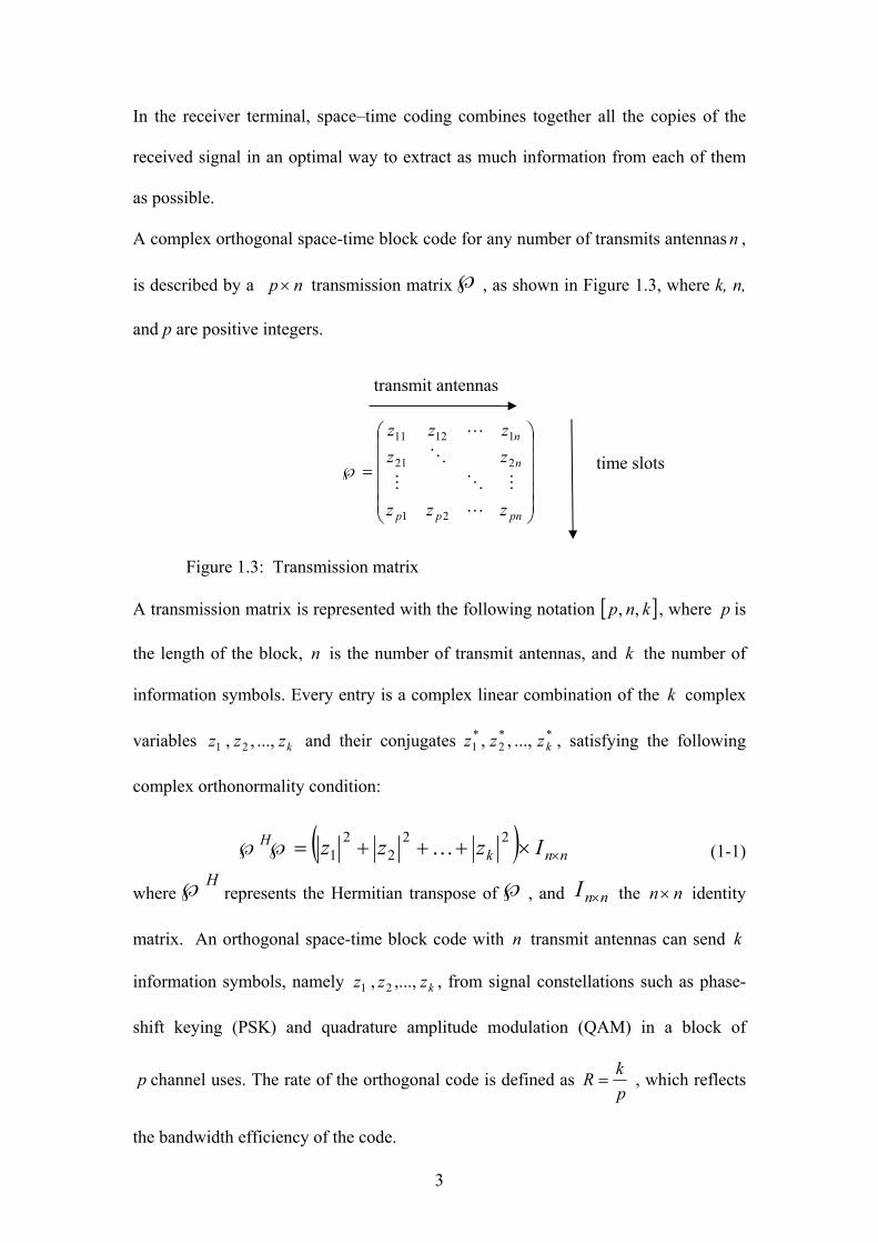
A complex orthogonal space-time block code for any number of transmits antennas n ,

is described by a np × transmission matrix ℘, as shown in Figure 1.3, where k, n,

and p are positive integers.

⎟⎟⎟⎟⎟

⎠

⎞

⎜⎜⎜⎜⎜

⎝

⎛

=℘

pnpp

n

n

zzz

zzzzz

L

MOM

O

L

21

221

11211

Figure 1.3: Transmission matrix A transmission matrix is represented with the following notation [ ]knp , , , where p is

the length of the block, n is the number of transmit antennas, and k the number of

information symbols. Every entry is a complex linear combination of the k complex

variables kzzz ..., , , 2 1 and their conjugates **2

*1 ..., , , kzzz , satisfying the following

complex orthonormality condition:

( ) nnkH Izzz ××+++=℘℘ 22

22

1 K (1-1)

where H℘ represents the Hermitian transpose of ℘, and nnI × the nn× identity

matrix. An orthogonal space-time block code with n transmit antennas can send k

information symbols, namely kzzz ,...,, 2 1 , from signal constellations such as phase-

shift keying (PSK) and quadrature amplitude modulation (QAM) in a block of

p channel uses. The rate of the orthogonal code is defined as pkR = , which reflects

the bandwidth efficiency of the code.

time slots

transmit antennas

4

The construction of high-rate orthogonal space-time block codes is an essential

problem in space-time block coding. The first complex orthogonal space-time block

code was proposed by Alamouti [10] as follows:

⎟⎟⎠

⎞⎜⎜⎝

⎛−

=℘ *1

*2

21

zzzz

(1-2)

for two transmit antennas [ ]knp ,, = [ ] 2 ,2 ,2 , which has full rate 122 ==R . Three,

four, five, and eight transmit antennas, with different rates were constructed by Liang

[12]. Obviously, a complex orthogonal space-time block code with high rate can

improve the bandwidth efficiency. Hence, in order to improve the bandwidth

efficiency of a complex orthogonal space-time block code for any given number of

transmit antennas, we need to apply the space-time block code with the highest rate

( R ) as possible. Orthogonal designs with maximal rates where demonstrated

successfully by Liang [12].

1.3 Antenna Theory An antenna is a device used for transmitting and/or receiving electromagnetic waves

which are operated in radio frequencies (RF), a range of 10 kHz to 300 GHz. The size

and shape of antennas are determined from the frequency of the signal they are

designed to receive. An antenna must be tuned to the same frequency band that the

radio system to which it is connected operates in, otherwise reception and/or

transmission will fail. Therefore, antennas couple electromagnetic energy from the

space to other mediums. In the recent years, due to the wireless cellular evolution

many antenna technologies were proposed which provide more quality, capacity, and

coverage. These types of antenna systems are the sectorized antenna systems,

diversity antenna systems and many others. For more information regarding antenna

5

theory refer to Ref. [13]. However, antennas are operated in a noisy environment

where many hostile effects should surpassed or minimize in order the communication

to be successful.

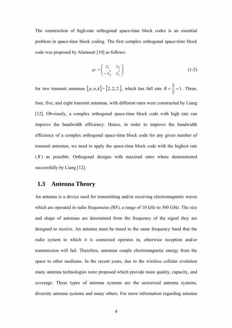
1.3.1 Multipath Interference Effect

Multipath interference is a phenomenon where two or more waves are transmitted at

the same time from a base station and travel through different paths towards the

receiving end (Figure 1.4); whereas, before the reception they interfere with each

other causing a phase shift.

Figure 1.4: The effect of multipath on a mobile user When the waves of multipath signals are out of phase, reduction in signal strength can

occur. This phenomenon is known as Rayleigh fading. As shown in Figure 1.5, fade

describes the loss of signal strength at the receiver by causing periodic attenuation. In

addition, due to the multiple reflections, the same signals could arrive at the receiver

end at different times. This effect arises a phenomenon called intersymbol

interference, where the receiver cannot sort the incoming information. As a result, the

bit error rate increases and distorts the incoming signal.

Path C

Base Station

Path A

Path B Mobile User

6

Figure 1.5: Representation of the Rayleigh fade effect on a user signal (Adapted from Ref. [14])

Another very important phenomenon is the co-channel interference (Figure 1.6),

where the same carrier frequency reaches the same mobile receiver from two separate

base stations.

Figure 1.6: Illustration of co-channel interference The signals that missed their intended destination become interference for the rest of

the users on the same frequency in the same or adjoin cells.

1.3.2 Doppler Effect

The Doppler Effect is the change in frequency of a wave that is perceived by an

observer moving towards or away from the source of the waves. It is well-known that

Doppler effects generated by high speed mobility are the major reason for the

1 4

3 1

3 2

2

4 1

1

7

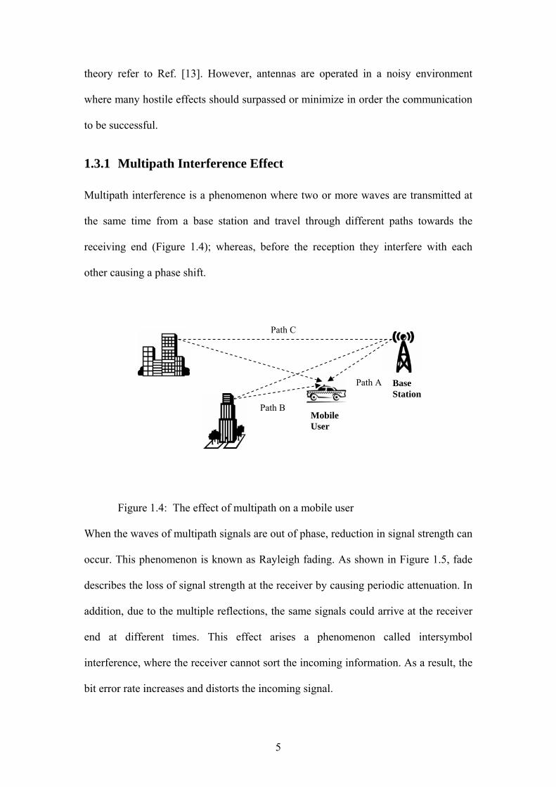
reduction of data rates in cellular systems. The Doppler Effect may occur from either

motion of the source (Figure 1.7) or motion of the receiver. This thesis will consider

the latter case, where the receiving end (mobile user) is in motion and the source (base

station) is stationary.

Figure 1.7: a) Stationary source b) Moving source

It is important to comprehend that the frequency of the signal that the source emits

does not actually change, but the wavelength (λ) does; consequently, the perceived

frequency is also affected. When the receiving end moves towards the base station the

receiving frequency becomes higher and when is receding the receiving frequency

becomes lower (see Figure 1.7).

The Doppler shift in frequency depends on the velocity between the source and the

receiver and on the speed of propagation of the signal. Doppler frequency is given by

the formula [15] :

cvff c ×±≈∆ (1-3)

where f∆ is the change in frequency, cf is carrier frequency, v is the speed

difference between the source and the receiver, and c is the speed of light in vacuum.

For the purpose of this paper the carrier frequency will be taken as 2 GHz as specified

in the Enhanced Data rates for GSM Evolution (EDGE) and the speed of light in

vacuum will be equal with sm 103c 8×= .

λ

(a) λ (b) λ

Low Freq.

High Freq.

8

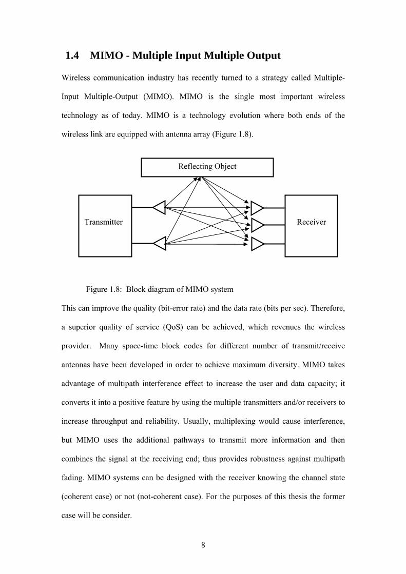
1.4 MIMO - Multiple Input Multiple Output Wireless communication industry has recently turned to a strategy called Multiple-

Input Multiple-Output (MIMO). MIMO is the single most important wireless

technology as of today. MIMO is a technology evolution where both ends of the

wireless link are equipped with antenna array (Figure 1.8).

Figure 1.8: Block diagram of MIMO system This can improve the quality (bit-error rate) and the data rate (bits per sec). Therefore,

a superior quality of service (QoS) can be achieved, which revenues the wireless

provider. Many space-time block codes for different number of transmit/receive

antennas have been developed in order to achieve maximum diversity. MIMO takes

advantage of multipath interference effect to increase the user and data capacity; it

converts it into a positive feature by using the multiple transmitters and/or receivers to

increase throughput and reliability. Usually, multiplexing would cause interference,

but MIMO uses the additional pathways to transmit more information and then

combines the signal at the receiving end; thus provides robustness against multipath

fading. MIMO systems can be designed with the receiver knowing the channel state

(coherent case) or not (not-coherent case). For the purposes of this thesis the former

case will be consider.

Transmitter

Receiver

Reflecting Object

9

1.4.1 Principles of MIMO Systems

An efficient way to improve data rate and transmission reliability over wireless links

is through the use of MIMO systems.

Figure 1.9: Basic spatial multiplexing scheme with 3-Tx antennas. Ai, Bi, and Ci represent symbol constellations (Adapted from Ref. [16])

Figure 1.9 shows an intuitive representation of how MIMO systems operate. A simple

bit sequence is decomposed into three independent sequences, which then are

transmitted simultaneously through multiple antennas. Bit sequences pass through

modulation and mapping process using various symbol constellations. The signals use

the same frequency spectrum and they naturally mix together in the wireless channel.

At the receiver, after having identified the mixing channel matrix (coherent case), the

individual bit streams are separated and estimated. This works in the same way as a

linear system of three equations. Therefore, each pair of transmit-receive antennas has

a single scalar channel coefficient, hence flat fading channel. A more detail

10

explanation about the functionality of MIMO systems is explained and illustrated in

Ref. [16] (also see later in this thesis for more details).

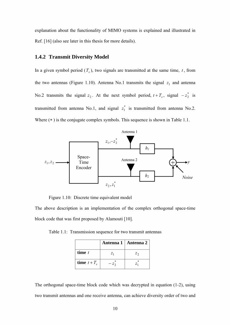
1.4.2 Transmit Diversity Model

In a given symbol period ( sT ), two signals are transmitted at the same time, t , from

the two antennas (Figure 1.10). Antenna No.1 transmits the signal 1z and antenna

No.2 transmits the signal 2 z . At the next symbol period, sTt + , signal *2z− is

transmitted from antenna No.1, and signal *1z is transmitted from antenna No.2.

Where (∗ ) is the conjugate complex symbols. This sequence is shown in Table 1.1.

Figure 1.10: Discrete time equivalent model The above description is an implementation of the complex orthogonal space-time

block code that was first proposed by Alamouti [10].

Table 1.1: Transmission sequence for two transmit antennas

Antenna 1 Antenna 2

time t 1z 2z

time sTt + *2z− *

1z

The orthogonal space-time block code which was decrypted in equation (1-2), using

two transmit antennas and one receive antenna, can achieve diversity order of two and

Noise

21, zz y

Space- Time

Encoder

h1

h2

Antenna 2

Antenna 1

*21, zz −

*12 , zz

11

full coding rate. This scheme can be generalized to n transmit antennas and one

receive antenna in order to achieve greater diversity order.

Chapter 2 introduces the system model which was used to analyze the performance of

various number of transmit antennas over time selective-fading channels.

1.5 Thesis Organization The remainder of this thesis has been organized as follows: Chapter 2 provides in

detail the system model that was used. Chapter 3 provides simulator features and

specifications of the modeled system. Chapter 4, 5, 6, and 7 present experimental

results for two, three, four, and five transmit antennas respectively base on the

proposed scheme. Finally, in Chapter 8, we conclude this thesis with a summary of

the results and we point to directions of future work.

12

Chapter 2

The System Model

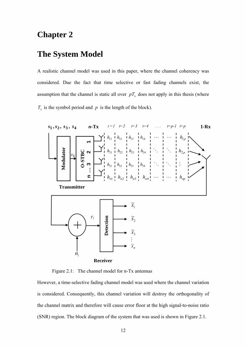
A realistic channel model was used in this paper, where the channel coherency was

considered. Due the fact that time selective or fast fading channels exist, the

assumption that the channel is static all over spT does not apply in this thesis (where

sT is the symbol period and p is the length of the block).

Figure 2.1: The channel model for n-Tx antennas However, a time-selective fading channel model was used where the channel variation

is considered. Consequently, this channel variation will destroy the orthogonality of

the channel matrix and therefore will cause error floor at the high signal-to-noise ratio

(SNR) region. The block diagram of the system that was used is shown in Figure 2.1.

ks

ri

11h 12h 13h 14h L L ph1

21h 22h 23h 24h O O ph2

31h 32h 33h 34h O O M

1nh 2nh 3nh 4nh L L nph

t =1 t=2 t=3 t=4 . . . t=p-1 t=p

Transmitter

Receiver in

Mod

ulat

or

O-S

TB

C

n .

.. 3

2

1

1~s

2~s

3~s M

ns~

Det

ectio

n

1-Rx n-Tx 1s , 2s , 3s , 4s

13

In order, to reduce the above error floor a high rate orthogonal time-space block codes

are introduced for the cases of two, three, four, and five transmit antennas [12]. The

orthogonal designs that will be presented in this thesis have a special structure.

⎟⎟⎟⎟⎟

⎠

⎞

⎜⎜⎜⎜⎜

⎝

⎛

−

−

−=℘

*2

*3

*1

*3

*1

*2

321

00

0

zzzz

zzzzz

Figure 2.2: Orthogonal time-space block code for 3-Tx antennas Each row has either only complex symbols or only conjugate (*) complex symbols, as

shown in Figure 2.2. This structure gives the flexibility to manipulate the complex

number properties in order to demodulate the receive signals.

2.1 Encoding We assume n transmit antennas and one receive antenna, where the information

symbols kzzz , , , 21 L are transmitted using complex orthogonal time-space block

codes [12]. All the complex information symbols are first grouped together by a

modulator and then passed trough an O-STBC encoder. Then they are transmitted

over =sT 1, 2, p,L symbol periods.

The receive signal ( ir ) at time i can be estimated by:

∑ +×==

n

jiijjii nchr

1 ... p, , where i ,321= (2-1)

where in is a complex additive white Gaussian noise (AWGN) with zero mean and

variance 2

2iσ , ijc equals with one of the following complex information symbols

kzzz ±±± ,,[ 2,1 L , ] ,, , **2

*1 kzzz ±±± L from O-STBC matrix (see Figure 1.3), and

14

jih denotes the time selective channel from the thj transmit antenna to the receive

antenna.

One of the best known models that have been used for a time variant flat-fading

channel is the Jake’s model [17], which is the following:

jiijiji whh )1()1( +×= −−α p ,, i

, n, , where j,21

21K

K

==

(2-2)

where jiw is noise which has complex Gaussian zero-mean with complex variance

2

2iσ per dimension, and it is statically independent of ( )1−ijh . The coefficient α can

be estimated by:

)2(0 sdi TfiJa ×××= π (2-3) where df is the Doppler frequency, sT is the information symbol duration, and

(.)0J is the 0th order Bessel function of the first kind (Figure 2.3).

Figure 2.3: Bessel Function of the first kind (Adapted from Ref. [18])

15

We need to give special attention to jiw where is another i.i.d complex Gaussian

random variable having zero mean and variance 2iσ and is statistically independent

of ( )1 −ijh . The variance of jiw can be calculated from the following:

( )2

12 1 −−= ii ασ (2-4)

where it depends on the variableα . The value of α depends on the terminal speed.

In order to find the Doppler frequency, df , we have to use the following formula:

)cV (ff cd ×= (2-5)

where cf corresponds to the carrier frequency, V is the speed of the mobile terminal,

and c is the speed of light in vacuum .

The information symbol duration sT can be found by:

ChipRateSFTs = (2-6)

where SF is the spreading factor. According to Universal Mobile Telecommunications

System (UMTS), sec

1084.3 6 chipsChipRate ×= and 128=SF .

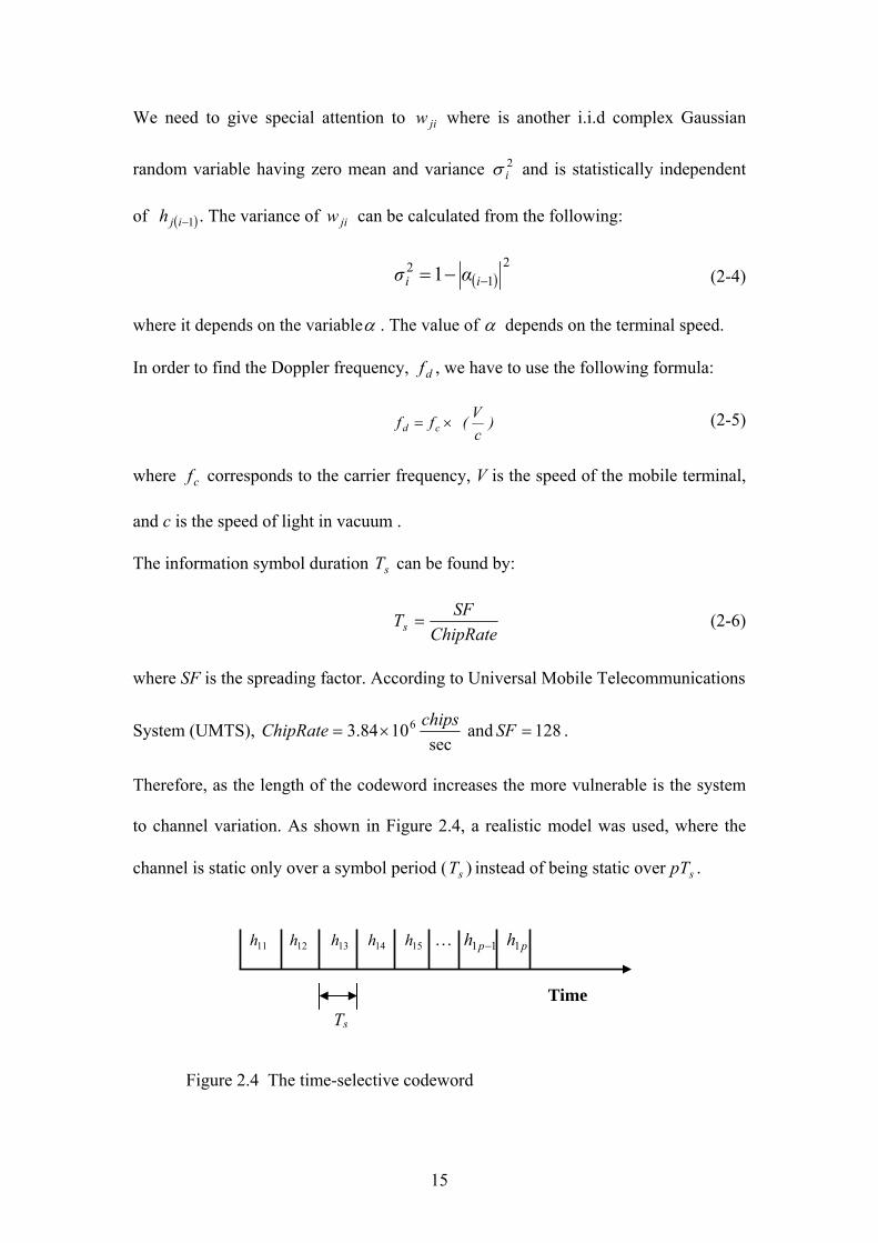
Therefore, as the length of the codeword increases the more vulnerable is the system

to channel variation. As shown in Figure 2.4, a realistic model was used, where the

channel is static only over a symbol period ( sT ) instead of being static over spT .

Figure 2.4 The time-selective codeword

Time Ts

11h 12h 13h 14h 15h … 11 −ph ph1

16

2.2 Decoding As mentioned above, the information was encoded based on the following model:

111 ×××× +×= p kkpp W S HY (2-7)

where Y is the received signal, H the channel, S the information, and W the noise. All

the variables are in a matrix form.

Given that the receiver knows the channel state information (coherent case), a simple

decoding algorithm was used:

[ ]11~

××× ××= pH

pkk YH d S (2-8)

where H denotes conjugate transpose (Hermitian) and the constant d is given by:

k

hhhd

pk22

122

11

1

+++=

L (2-9)

17

Chapter 3

Simulation Methodology

MATLABTM Release 14, V 7.0 was used as a simulator tool in order to perform the

simulation experiments.

3.1 Simulator

MATLABTM is a software package for high-performance in technical computing,

integrating programming, visualization, and computation in a very user-friendly

environment. Best of all, it also provides extensibility and flexibility with its own

high-level programming language. Common uses of MATLABTM involve [19]:

(a) Mathematics (Arrays and matrices, linear algebra, etc.)

(b) Programming development (Function, data structures, etc.)

(c) Modeling and simulation (Signal Processing etc.)

(d) Data analysis (statistics etc.)

(e) Visualization (graphics, animation etc.)

All the simulations were performed by automation programs which were created by

me. The whole simulation program was divided in sub-functions which were built in

M-files form, ∗ .m extension. More details about the structure of the software are

shown in Figure 3.1.

3.2 Components of Simulation

The following components were modeled, through the simulations:

1. Complex information symbols signals

2. Flat-fading channels (Jake’s model [17])

18

Figure 3.1: Flowchart of the m-file functions of the simulation software

START

STOP

Given • A complex O-STBC design ],,[ knp • System Model

Find Block error rate, Symbol error rate, and Bit error rate

Given • Two vectors of the same

length Find number of positions in which components are not the same

Given • A complex vector 1×k

Find transmission matrix (H)

Given • A complex vector

Find its components indexes in counter-clock manner

Main function • Initialize variables

o Signal-to-Noise Ratio ( dB 360 − ) o Number of realizations ( 6105× ) o Number of errors (1000)

• Load output matrix • Testing invalid outputs • Save and print results

Given • Two binary sequences

Find Hamming distance

do { # realizations }

19

3. Doppler effect

4. White Gaussian Noise

5. Terminal speed

3.3 Constellations The complex information symbols kzzz ±±± ,, [ 2,1 L , ] ,, , **

2*1 kzzz ±±± L are

transmitted using complex orthogonal time-space block codes. The information

symbols are randomly selected from 4-PSK or/and 8-PSK constellations accordingly

in order to achieve transmission of two bits per channel use (Figure 3.2).

Figure 3.2: a) 4-PSK constellation b) 8-PSK constellation (Phase Shift Key) The representations of the information symbols are randomly selected from the above

constellations and the bit mapping of the signals are built in an array form as shown

below:

1> PSK4_constellation= [ 2> 1 i -1 -i 3>]; 4> 5> PSK4_bitmapping= [ 6> 00 01 11 10 7>]; 8> 9> %------------------------------------------------------------------------------------

2 3

1

4

3 1

2 4

5

7

6 8

(a) (b)

20

10> PSK8_constellation= [ 11>1 1/sqrt(2)+i*1/sqrt(2) i -1/sqrt(2)+i*1/sqrt(2) -1 -1/sqrt(2)-i*1/sqrt(2) -i 1/sqrt(2)-12> i*1/sqrt(2) 13>]; 15> 16> PSK8_bitmapping= [ 17> 000 001 101 100 110 111 011 010 18>];

3.4 Terminal Speeds

The following seven vehicle speeds 0, 25, 50, 75, 150, 200, and 250h

km were used to

calculate the Doppler frequencies and their corresponding constants sd Tf × .

sT is the symbol period and equals with s.

610843128×

and df is the Doppler

frequency shift and can be calculated using the equations 1-3, 2-3, and 2-5 (see Table

3.1).

Table 3.1: Vehicle speeds with their corresponding constants

Vehicle Speed (h

km ) sd Tf ×

1 0 0 2 25 0.001543 3 50 0.003086 4 75 0.004630 5 150 0.009300 6 200 0.012300 7 250 0.015400

It’s obvious, that the value of ia depends on the applications. Recalling the formula

of ia

)2(0 sdi TfiJa ×××= π (3-1)

21

we can realize that the terminal speed is the major factor that determines the value of

ia . Using the above formula it can be shown that for speeds less thanh

km 150

) 150 (h

kmV ⟨ , iα is greater than 0.9991 ( 0.9991 ⟩ia and assuming that 4 ⟨i ).

Consequently, as the number of transmit antennas increases the length of the block

increases as well. In addition, as the terminal speed increases more channel variation

occurs. The consequences of the above factors result to an irreducible error floor in

the BER curves at the high signal-to-noise ratio region.

Considering the above restrictions and base on realistic scenarios the range of the

above speeds (h

km 2500 − ) was chosen among many others in order to determine the

performance of different multiple transmit antennas. For instance, high speeds trains

in Europe can easily reach 250 kilometers per hour. On the other hand, indoor

networks can be built where the receiver is stationary (h

km 0 ).

3.5 Simulation Parameters

All the simulation parameters that have been used in this thesis are base on European

Telecommunication Standards [20].

• Carrier Frequency: GHz 2

• Transmission Rate: sec

144 kbits

• Terminal Speeds: h

km 2500 −

• Channel Realizations: 6105×

• Signal to Noise Ratio (SNR): dB 360 −

22

• Bit Error Rate (BER): 6100 −−

• Chip Rate:sec

chips 1084.3 6×

• Spreading Factor (SF)=128

23

Chapter 4

Two Transmit Antennas

This chapter presents performance results of two transmit antennas and one receive

antenna over the impact of time-varying channels base on the terminal speeds.

4.1 Channel Matrix Calculations

The remarkable Alamouti-coded symbol matrix was used for two transmit antennas,

for the time intervals 1 , +tt [10].

⎟⎟⎠

⎞⎜⎜⎝

⎛−

=℘ *1

*2

21

zzzz

z (4-1)

Alamouti scheme has low complexity and it can achieve full rate 122==R

( [ ]knp ,, = [ ]2 ,2 ,2 ).

The complex modulation symbols kz are arranged based on a transmit matrix z℘ . It

is important to mention that the power of each symbol is normalized, 1)( 2 =Ε kz . Let

1h and 2h be the channels from the two transmit antennas to the receive antenna,

respectively. In all orthogonal space-time block schemes, a crucial assumption was

considered, where 1h and 2h are constants over two consecutive symbol periods. This

thesis, will not consider this assumption, rather the channel state will vary from

symbol to symbol, as shown in Figure 4.1.

2 ,1 )1()( =+⋅≠ iwherethth ii (4-2)

24

Figure 4.1: Transmission model for 2-Tx antennas

At times:

1=t 12211111 wzhzhy +⋅+⋅= (4-3)

2=t *22

*121

*22

*22

*212

*1222 wzhzhywzhzhy +⋅−⋅=⇒+⋅−⋅= (4-4)

From equations 4-3 and 4-4 the receive signal in matrix form is:

⎥⎦

⎤⎢⎣

⎡+⎥

⎦

⎤⎢⎣

⎡⋅⎥

⎦

⎤⎢⎣

⎡−

=⎥⎦

⎤⎢⎣

⎡*2

1

2

1*12

*22

2111*2

1

ww

zz

hhhh

yy

(4-5)

where the dimensions of matrix/vectors are: 12122212 ×××× +×= W S HY .

As you can see from the above calculations the receive signal is given by:

wsHy +⋅= ~~ (4-6)

where s is the signal vector, T21 ][ zzs = , w is the noise vector, T*

21 ][ www = ,

and H~ is the new mortified coded channel matrix, ⎥⎦

⎤⎢⎣

⎡−

= *12

*22

2111~hh

hhH .

To detect the original information symbols, we take advantage the orthogonal

structure of H~ , so the retrieve symbols can be found by:

( )ws

hhhhyHs H ~

2 ~ ~~

222

221

212

211 +⋅

+++=⋅= (4-7)

4.2 Simulation Results

The following graphs illustrate simulation results in terms of bit, symbol, and block

error probability versus signal-to-noise ratio (SNR) for two transmit antennas and one

11h 1z 12h *2z−

21h 2z 22h *1z

t=1 t=2

1-Rx2-Tx

25

receive antenna based on seven different vehicle speeds 0, 25, 50, 75, 150, 200, and

250h

km , for transmission of 2 bits per channel use. The transmission using

Alamouti’s scheme [10] for two transmit antennas employs the 4-PSK constellation.

Figure 4.2: Bit, symbol, and block error probability versus signal-to-noise ratio (SNR) for 2-Tx antennas base on vehicle speed 0, 25, 50, 75, 150, 200, and 250 km/h, respectively. (Figure Continue)

(c) 50 km/h (d) 75 km/h

(a) 0 km/h (b) 25 km/h

26

(g) 250 km/h

(e) 150 km/h (f) 200 km/h

27

4.3 Performance Evaluation

Through analysis and simulations, we present the performance of two transmit

antennas and one receive antenna over time-varying fading channels. For comparison

and readability purposes we plot all the BER curves for all the aforementioned speeds,

as shown in Figure 4.3.

Figure 4.3: BER comparisons between different values of speeds, for 2-Tx antennas

Assuming that the receiver has perfect knowledge of the channel, a very low

complexity decoding algorithm is proposed. At low vehicle speeds or slow fading

scenarios (h

kmV 75 ⟨ ), our simulations indicated that the bit error probability has very

low variation below the bit error rate of 510 − . However, above 510− the bit error

remains the same for vehicle speeds below 75h

km . Consequently, the scheme

28

performance of the proposed decoding algorithm is excellent and shows no error floor

at all at low vehicle speeds and under the presence of channel variation. On the other

hand, when the vehicle speed is equal to or higher than 150h

km the receiver exhibits

a progressively severe irreducible error floor in the high SNR region. At low vehicle

speeds, the assumption that the channel remains static over the length of the codeword

is reasonable; whereas, our simulations show that channel variation at higher speeds

destroys the orthogonality of transmission matrix leading to irreducible error floor in

the high SNR region. As shown in the graph, the higher signal-to-noise ratio the lower

the number of errors. Therefore, the desired low error bit probability comes with a

costly price of high SNR. This undesirable price will be minimized by the addition of

more transmit antennas, which will be discussed in the following chapters.

29

Chapter 5

Three Transmit Antennas

This chapter exhibits performance results for three transmit antennas and one receive

antenna over time-selective fading channels, according to user vehicle speeds.

5.1 Channel Matrix Calculations

Using the Adams-Lax-Philips [21] construction matrix techniques, which are clearly

demonstrated in Ref. [12], the following orthogonal space-time block code was

chosen for the simulations of the three antennas.

⎟⎟⎟⎟⎟

⎠

⎞

⎜⎜⎜⎜⎜

⎝

⎛

−−−

=℘

*2

*3

*1

*3

*1

*2

321

00

0

zzzz

zzzzz

z (5-1)

This O-STBC has rate of 43

==pkR ( [ ]knp , , = [ ]3 ,3 ,4 ) and it has a special

structure where each row has either only complex symbols or only conjugate (∗ )

complex symbols. This structure gives the flexibility to use the complex number

properties in order to demodulate the receive signals. The complex modulation

symbols ] , , , ,[ *3

*2

*1,321 zzzzzz are transmitted and arranged according to the

transmission matrix z℘ . During the time intervals, t, t+1, t+2, and t+3 the channel

state varies over the length of the codeword. Let iii hhh 321 , , be the channel for the

transmit antennas one, two, and three respectively, where 4 ,3 21 ,, i = , as shows in

Figure 5.1.

30

Figure 5.1: Transmission model for 3-Tx antennas

At times:

1=t 13312211111 wzhzhzhy +⋅+⋅+⋅= (5-2)

2=t *22

*121

*22

*2232

*212

*1222 00 wzhzhywhzhzhy ++⋅−⋅=⇒+⋅+⋅−⋅= (5-3)

3=t *33

*131

*33

*33

*133

*313233 00 wzhzhywzhzhhy ++⋅−⋅=⇒+⋅+⋅−⋅= (5-4)

4=t *43

*242

*34

*44

*234

*324144 00 wzhzhywzhzhhy ++⋅−⋅=⇒+⋅+⋅−⋅= (5-5)

From equations 5-2, 5-3, 5-4, and 5-5 the receive signal in matrix form is:

⎥⎥⎥⎥

⎦

⎤

⎢⎢⎢⎢

⎣

⎡

+⎥⎥⎥

⎦

⎤

⎢⎢⎢

⎣

⎡⋅

⎥⎥⎥⎥

⎦

⎤

⎢⎢⎢⎢

⎣

⎡

−−

−=

⎥⎥⎥⎥

⎦

⎤

⎢⎢⎢⎢

⎣

⎡

*4

*3

*2

1

3

2

1

*24

*34

*13

*33

*12

*22

312111

*4

*3

*2

1

00

0

wwww

zzz

hhhh

hhhhh

yyyy

(5-6)

where the dimensions of matrix/vectors are: 14133414 ×××× +×= W S HY .

As you can see from the above calculations the receive signal is given by:

wsHy +⋅= ~~ (5-7)

where s is the signal vector, T321 ][ zzzs = , w is the noise vector,

T*4

*3

*21 ][ wwwww = , and H~ is the new mortified orthogonal coded channel

matrix.

t=1 t=2 t=3 t=4

11h 1z 12h *2z− 13h *

3z− 14h 0

21h 2z 22h *1z 23h 0 24h *

3z−

31h 3z 32h 0 33h *1z 34h *

2z

3-Tx 1-Rx

31

⎥⎥⎥⎥

⎦

⎤

⎢⎢⎢⎢

⎣

⎡

−−

−=℘

*24

*34

*13

*33

*12

*22

312111

00

0

hhhh

hhhhh

h (5-8)

The detection procedure is the same as it is described in chapter 2 and chapter 4.

5.2 Simulation Results

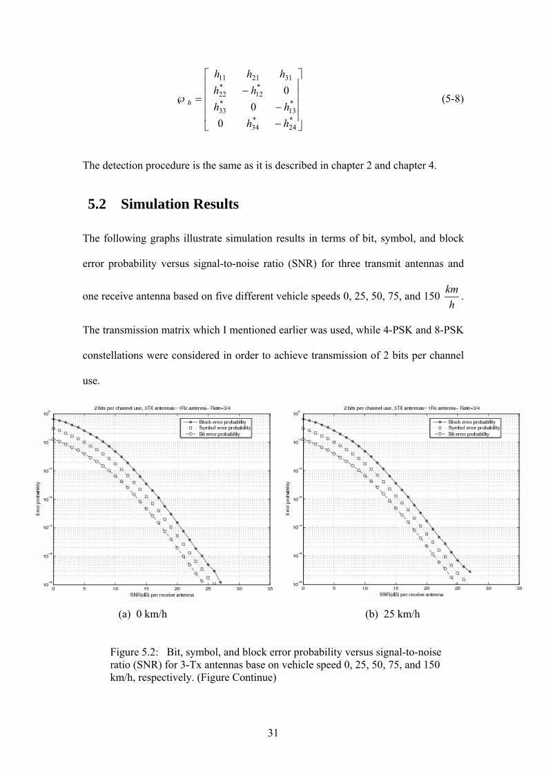
The following graphs illustrate simulation results in terms of bit, symbol, and block

error probability versus signal-to-noise ratio (SNR) for three transmit antennas and

one receive antenna based on five different vehicle speeds 0, 25, 50, 75, and 150h

km .

The transmission matrix which I mentioned earlier was used, while 4-PSK and 8-PSK

constellations were considered in order to achieve transmission of 2 bits per channel

use.

Figure 5.2: Bit, symbol, and block error probability versus signal-to-noise ratio (SNR) for 3-Tx antennas base on vehicle speed 0, 25, 50, 75, and 150 km/h, respectively. (Figure Continue)

(a) 0 km/h (b) 25 km/h

32

5.3 Performance Evaluation

Based on analysis and simulations, we present the BER performance of the proposed

decoder for three transmit antennas and one receive antenna over time-selective

fading channels. For comparison and readability purposes we plot all the BER curves

for all the above mentioned speeds, as shown in Figure 5.3.

(c) 50 km/h (d) 75 km/h

(e) 150 km/h

33

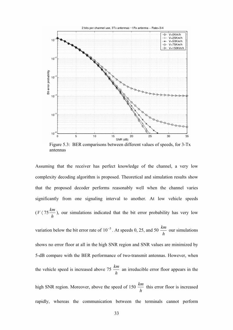
Figure 5.3: BER comparisons between different values of speeds, for 3-Tx antennas

Assuming that the receiver has perfect knowledge of the channel, a very low

complexity decoding algorithm is proposed. Theoretical and simulation results show

that the proposed decoder performs reasonably well when the channel varies

significantly from one signaling interval to another. At low vehicle speeds

(h

kmV 75 ⟨ ), our simulations indicated that the bit error probability has very low

variation below the bit error rate of 510 − . At speeds 0, 25, and 50h

km our simulations

shows no error floor at all in the high SNR region and SNR values are minimized by

5-dB compare with the BER performance of two-transmit antennas. However, when

the vehicle speed is increased above 75h

km an irreducible error floor appears in the

high SNR region. Moreover, above the speed of 150h

km this error floor is increased

rapidly, whereas the communication between the terminals cannot perform

34

successfully. As shown in Figure 5.3, using three transmit antennas we achieved the

same bit error probability with lower SNR values, compared with the two transmit

antenna scheme (Figure 4.3). Overall, three antennas can perform better in some

applications but on the other hand, hostile error floor effects must be considered at

high vehicle speeds.

In the next chapter, we will consider a scheme where four transmit antennas and one

receive antenna take place.

35

Chapter 6

Four Transmit Antennas

This chapter presents performance results for four transmit antennas and one receive

antenna over time-varying channels based on the terminal speeds. In the section 6.2

simulation results were built with 1.5 bits per channel use, where in the section 6.3

2 bits per channel use was considered.

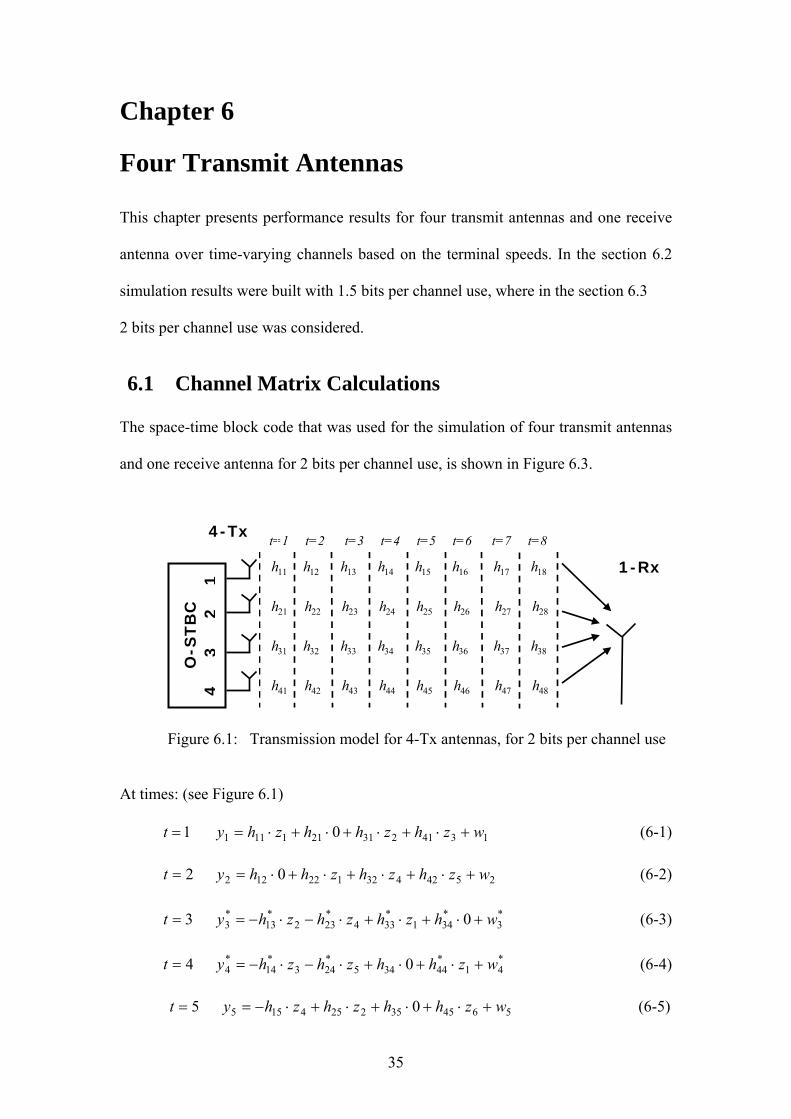
6.1 Channel Matrix Calculations The space-time block code that was used for the simulation of four transmit antennas

and one receive antenna for 2 bits per channel use, is shown in Figure 6.3.

Figure 6.1: Transmission model for 4-Tx antennas, for 2 bits per channel use

At times: (see Figure 6.1)

1=t 1341231211111 0 wzhzhhzhy +⋅+⋅+⋅+⋅= (6-1)

2=t 2542432122122 0 wzhzhzhhy +⋅+⋅+⋅+⋅= (6-2)

3=t *3

*341

*334

*232

*13

*3 0 whzhzhzhy +⋅+⋅+⋅−⋅−= (6-3)

4=t *41

*44345

*243

*14

*4 0 wzhhzhzhy +⋅+⋅+⋅−⋅−= (6-4)

5=t 5645352254155 0 wzhhzhzhy +⋅+⋅+⋅+⋅−= (6-5)

1-Rx

O-S

TB

C

4 3

2

1

11h 12h 13h 14h 15h 16h 17h 18h

21h 22h 23h 24h 25h 26h 27h 28h

31h 32h 33h 34h 35h 36h 37h 38h

41h 42h 43h 44h 45h 46h 47h 48h

t=1 t=2 t=3 t=4 t=5 t=6 t=7 t=84-Tx

36

6=t *62

*463

*366

*2616

*6 0 wzhzhzhhy +⋅+⋅−⋅−⋅= (6-6)

7=t 7476373275177 0 whzhzhzhy +⋅+⋅−⋅+⋅−= (6-7)

8=t *84

*485

*38286

*18

*8 0 wzhzhhzhy +⋅+⋅−⋅−⋅= (6-8)

⎥⎥⎥⎥⎥⎥⎥⎥⎥⎥⎥

⎦

⎤

⎢⎢⎢⎢⎢⎢⎢⎢⎢⎢⎢

⎣

⎡

+

⎥⎥⎥⎥⎥⎥⎥⎥

⎦

⎤

⎢⎢⎢⎢⎢⎢⎢⎢

⎣

⎡

⋅

⎥⎥⎥⎥⎥⎥⎥⎥⎥⎥⎥

⎦

⎤

⎢⎢⎢⎢⎢⎢⎢⎢⎢⎢⎢

⎣

⎡

−−−−−

−−−

−−

=

⎥⎥⎥⎥⎥⎥⎥⎥⎥⎥⎥

⎦

⎤

⎢⎢⎢⎢⎢⎢⎢⎢⎢⎢⎢

⎣

⎡

*8

7

*6

5

*4

*3

2

1

6

5

4

3

2

1

*18

*38

*48

371727

*26

*36

*46

451525

*24

*14

*44

*23

*13

*33

423222

413111

*8

7

*6

5

*4

*3

2

1

000000

000000

000000000000

wwwwwwww

zzzzzz

hhhhhhhhh

hhhhhh

hhhhhh

hhh

yyyyyyyy

(6-9)

where the dimensions of matrix/vectors are: 18166818 ×××× +×= W S HY .

And again the receive signal is given by:

wsHy +⋅= ~~ (6-10) where s is the signal vector, T

654321 ][ zzzzzzs = , w is the noise

vector, T*87

*65

*4

*321 ][ wwwwwwwww = , and ~H is the new orthogonal

mortified coded channel matrix (equation 6-11).

⎥⎥⎥⎥⎥⎥⎥⎥⎥⎥⎥

⎦

⎤

⎢⎢⎢⎢⎢⎢⎢⎢⎢⎢⎢

⎣

⎡

−−−−−

−−−

−−

=℘

*18

*38

*48

371727

*26

*36

*46

451525

*24

*14

*44

*23

*13

*33

423222

413111

000000

000000

000000000000

hhhhhhhhh

hhhhhh

hhhhhh

hhh

h (6-11)

37

To detect the original information symbols, we take advantage the orthogonal

structure of H~ , so the retrieve symbols can be found by :

yHs H ~ ~~ ⋅= (6-12)

6.2 Comparison of Performance of Two O-STBC for Four Transmit Antennas

Orthogonal designs have been used as space–time block codes for wireless

communications with multiple transmit antennas )( n . This section of the chapter

presents a comparison of performance of two orthogonal space-time block codes with

different rates, 84 1 =R and

86 2 =R , for four transmit antennas over time-selective

fading channels. It is shown that under time-selectiveness and once the vehicle speed

rises above a certain value, the code with rate of 86 is much more efficient than the

code with rate84 [12, 22].

6.2.1 Orthogonal Designs The aim of this section is to introduce a new orthogonal space-time code design,

which minimizes the floor error that arises due to the terminal speed. The orthogonal

designs that will be presented in this chapter have a special structure. Each row has

either only complex symbols or only conjugate (∗ ) complex symbols (Figure 6.2 and

Figure 6.3). This structure gives the flexibility to manipulate the complex number

properties in order to demodulate the receive signals. The new orthogonal design has

many advantages over the conventional code [22] that has been used so far.

38

6.2.2 The Conventional O-STBC This space-time block code, (Figure 6.2) can find application for 4 transmit antennas

)(n to send 4 information symbols )(k in a block of 8 channel uses )( p . The rate of

this orthogonal code is therefore, 21

84===

pkR [22].

⎟⎟⎟⎟⎟⎟⎟⎟⎟⎟⎟

⎠

⎞

⎜⎜⎜⎜⎜⎜⎜⎜⎜⎜⎜

⎝

⎛

−−−−

−−

−−−−

−−

=℘

*1

*2

*3

*4

*2

*1

*4

*3

*3

*4

*1

*2

*4

*3

*2

*1

1234

2143

3412

4321

ZZZZZZZZ

ZZZZZZZZZZZZZZZZ

ZZZZZZZZ

Figure 6.2: The conventional code [p, n, k] = [8, 4, 4]

6.2.3 The New High-Rate O-STBC The new design of transmission matrix for 4 transmit antennas of size 48× is given

in Figure 6.3. This matrix is clearly an orthogonal space-time block code and sends

6 =k information symbols in a block of 8 =p channel uses. The rate of this

orthogonal code is therefore, 43

86===

pkR [12].

⎟⎟⎟⎟⎟⎟⎟⎟⎟⎟⎟

⎠

⎞

⎜⎜⎜⎜⎜⎜⎜⎜⎜⎜⎜

⎝

⎛

−−−−−

−−−−−

=℘

*4

*5

*6

635

*2

*3

*6

624

*1

*5

*3

*1

*4

*2

541

321

00

000

00

0

ZZZZZZ

ZZZZZZZZZ

ZZZZZZZZZ

Figure 6.3: The new High-Rate O-STBC [p, n, k] = [8, 4, 6]

39

6.2.4 Comparison of the Orthogonal Designs Clearly, the new orthogonal design has a greater rate than the conventional code.

Consequently, the new high rate orthogonal design can achieve bigger diversity gain

by transmitting additional two more information symbols. Another big advantage of

the new orthogonal design is that in eight symbol periods ( sT ) transmits zero

(nothing), which saves power consumption to the transmitter. The simulations show

that the new orthogonal design can efficiently reduce the error floor at the high signal-

to-noise ratio (SNR) region. In addition, it provides better performance in high vehicle

speed values.

6.2.5 Simulation Results for 1.5 Bits per Channel Use

The following section provides simulation results for the performance of the above

orthogonal space-time block codes. The new orthogonal design code with rate 43 is

compared with the conventional code, which has rate21 . The transmission model that

was used it is described in detail in chapter 2 and is similar with the transmission

model for wireless communication systems with multiple antennas as described in

Ref. [23]. A simple decoding algorithm under the assumption that the receiver knows

the channel state information is also described in chapter 2. The receiver estimates the

transmitted bits by using the signals of the receive antennas (coherent case). Figure

6.5 and Figure 6.6 show bit error rates (BER), for transmission of 1.5 bits per channel

use for four transmit antennas and one receive antenna, with rates 84 and

86 ,

respectively. In order to achieve a transmission with 1.5 bits per channel use, 8-PSK

(Phase Shift Key) constellation for the conventional orthogonal design and 4-PSK

40

constellation for the new orthogonal design were used. Channel matrix H was

generated using the equation 2-2, Jake’s model [17]. Each graph in Figure 6.4

presents the performance results for terminal speeds 0, 25, 50, and 75h

km . The bit

error rate at each SNR )/( 0NEb point is averaged over 6105× channel realizations.

Figure 6.4: The BER vs. SNR performance between the two orthogonal designs for terminal speeds 0, 25, 50, and 75 km/h respectively

(a) 0 km/h (b) 25 km/h

(c) 50 km/h (d) 75 km/h

41

Figure 6.5: The BER performance of the O-STBC with rate =84

Figure 6.6: The BER performance of the O-STBC with rate =86

42

6.2.6 Conclusions The section 6.2 has shown simulation results for the performance of the new

orthogonal space-time block code. It is clearly shown that the new orthogonal design

(Figure 6.6) has better performance compared with the conventional orthogonal

design (Figure 6.5). It reduces efficiently the error floor at the high signal-to-noise

ratio region, especially when the terminal speed is 50h

km (Figure 6.4c).

6.3 Simulation Results for 2 Bits per Channel Use

The graphs in Figure 6.7 illustrate simulation results in terms of bit, symbol, and

block error probability versus signal-to-noise ratio (SNR) for four transmit antennas

and one receive antenna base on four different vehicle speeds 0, 25, 50, and 75h

km ,

for transmission of 2 bits per channel use. The orthogonal transmission matrix that

was used is the one that was demonstrated in Figure 6.3. It’s important to mention,

that in order to achieve a transmission rate of 2 bits per channel use, 4-PSK and 8-

PSK constellations where used. Therefore, two symbols where selected from 4-PSK

constellation and four symbols from 8-PSK constellation since the orthogonal design

has rate of86 ==

pkR .

6.4 Performance Evaluation The analysis and simulations, for four transmit antennas and one receive antenna have

shown that for vehicle speeds above 25 h

km a significant amount of error floor

appears at high regions of SNR, as shown in Figure 6.8.

43

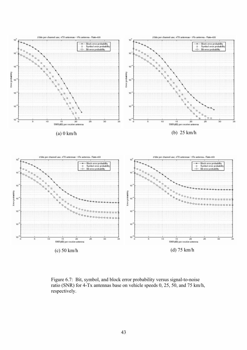
Figure 6.7: Bit, symbol, and block error probability versus signal-to-noise ratio (SNR) for 4-Tx antennas base on vehicle speeds 0, 25, 50, and 75 km/h, respectively.

(b) 25 km/h (a) 0 km/h

(c) 50 km/h (d) 75 km/h

44

Figure 6.8: BER comparisons between different values of speeds, for 4-Tx antennas

On the other hand, the scheme performance below 25h

km is excellent and shows no

error floor at all, under the presence of channel variation. Consequently, when the

terminals speeds are kept below 25h

km , a very good performance appears where the

bit error probability is very low at low signal-to-noise ratio areas. The performance of

this scheme has shown that it can find real applications, which are discussed in detail

in chapter 8.

45

515*8

*9

*10

*6

*7

*10

*5

*7

*9

*5

*6

*8

10947

*3

*4

*10

10836

*2

*4

*9

*2

*3

*8

9825

*1

*7

*4

*1

*6

*3

*1

*5

*2

7651

4321

0000

00000

00000

000

000000

00

×⎟⎟⎟⎟⎟⎟⎟⎟⎟⎟⎟⎟⎟⎟⎟⎟⎟⎟⎟⎟⎟⎟

⎠

⎞

⎜⎜⎜⎜⎜⎜⎜⎜⎜⎜⎜⎜⎜⎜⎜⎜⎜⎜⎜⎜⎜⎜

⎝

⎛

−−

−−

−−−−−

−−−−−−

−−−−−−−

=℘

zzzzzzzzz

zzzzzzz

zzzzzzzzzz

zzzzzzzzzz

zzzzzz

zzzzzzzz

z

Chapter 7 Five Transmit Antennas This chapter demonstrates performance results for five transmit antennas and one

receive antenna over time-selective fading channels, according on user vehicle speeds.

7.1 Channel Matrix Calculations

An outstanding orthogonal matrix construction procedure was demonstrated in Ref.

[12], where using the proposed construction matrix technique, the following

orthogonal space-time block code was obtained.

(7-1)

46

The above orthogonal space-time block channel matrix has rate of 1510

==pkR

( [ ]knp , , = [ ]10 ,5 ,15 ) and it is used for five transmit antennas. The complex

modulation symbols are transmitted and arranged according to the above transmission

matrix z℘ in such a way that each row has either only complex symbols or only

conjugate (∗ ) complex symbols. During the fifteen time intervals, channel state varies

over the length of the codeword. Let iiiii hhhhh 54321 , , , , be the channel for the

transmit antennas one, two, three, four, and five, respectively, where 15 , 21 L,, i = .

The corresponding orthogonal channel matrix is shown below:

(7-2)

⎥⎥⎥⎥⎥⎥⎥⎥⎥⎥⎥⎥⎥⎥⎥⎥⎥⎥⎥⎥⎥⎥

⎦

⎤

⎢⎢⎢⎢⎢⎢⎢⎢⎢⎢⎢⎢⎢⎢⎢⎢⎢⎢⎢⎢⎢⎢

⎣

⎡

−−−

−−−−−−

−−−−

−−−

−−−−

−−

=℘

*315

*415

*515

*114

*414

*514

*113

*313

*513

*112

*312

*412

411311111211

*210

*410

*510

59391929

*28

*38

*58

*27

*37

*47

56461626

*25

*15

*35

*24

*14

*44

*23

*13

*33

52423222

51413111

00000000000000

00000000000000

0000000000000000000

00000000000000000000000000000000000000000000000000000

hhhhhh

hhhhhh

hhhhhhhhhhh

hhhhhh

hhhhhhh

hhhhhh

hhhhhhhh

h

47

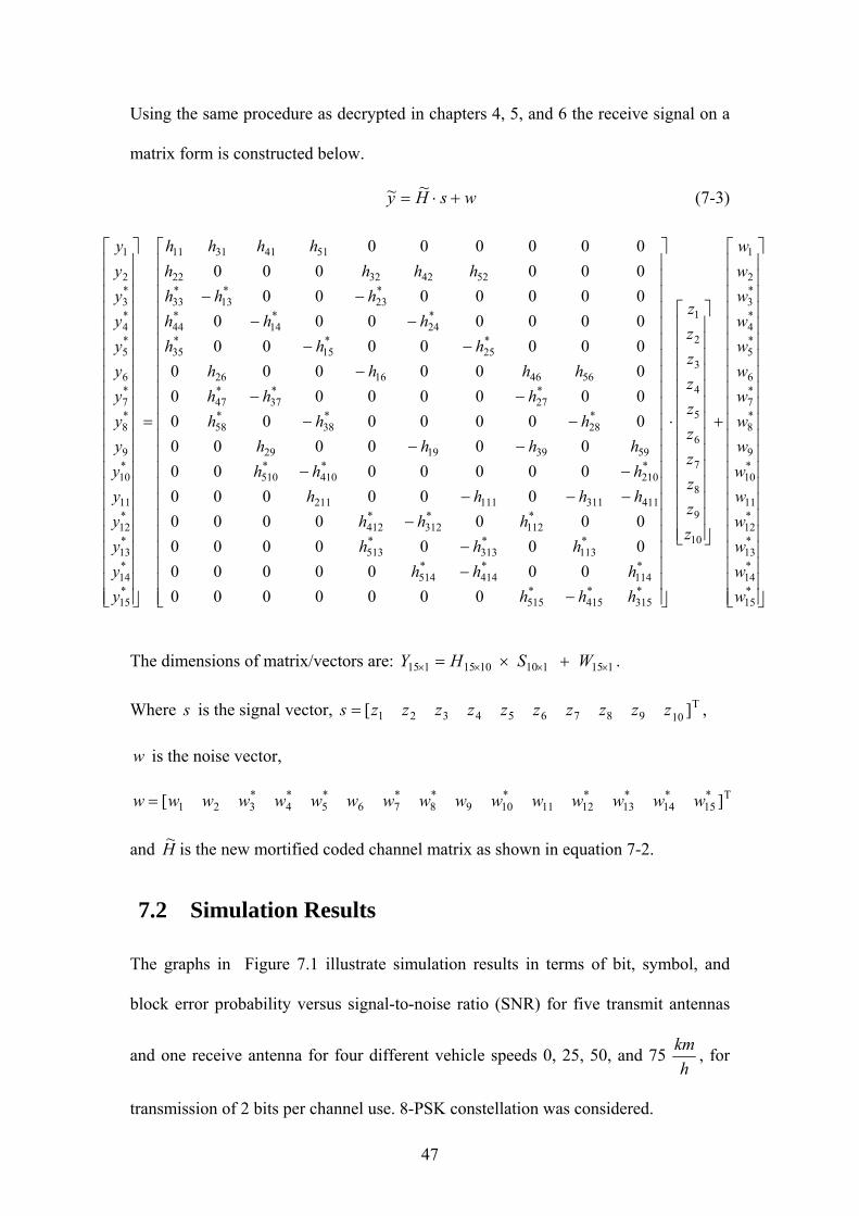
Using the same procedure as decrypted in chapters 4, 5, and 6 the receive signal on a

matrix form is constructed below.

wsHy +⋅= ~~ (7-3)

The dimensions of matrix/vectors are: 1151101015115 ×××× +×= W S HY .

Where s is the signal vector, T10987654321 ][ zzzzzzzzzzs = ,

w is the noise vector,

T*15

*14

*13

*1211

*109

*8

*76

*5

*4

*321 ][ wwwwwwwwwwwwwwww =

and H~ is the new mortified coded channel matrix as shown in equation 7-2.

7.2 Simulation Results

The graphs in Figure 7.1 illustrate simulation results in terms of bit, symbol, and

block error probability versus signal-to-noise ratio (SNR) for five transmit antennas

and one receive antenna for four different vehicle speeds 0, 25, 50, and 75h

km , for

transmission of 2 bits per channel use. 8-PSK constellation was considered.

⎥⎥⎥⎥⎥⎥⎥⎥⎥⎥⎥⎥⎥⎥⎥⎥⎥⎥⎥⎥⎥⎥

⎦

⎤

⎢⎢⎢⎢⎢⎢⎢⎢⎢⎢⎢⎢⎢⎢⎢⎢⎢⎢⎢⎢⎢⎢

⎣

⎡

+

⎥⎥⎥⎥⎥⎥⎥⎥⎥⎥⎥⎥⎥⎥

⎦

⎤

⎢⎢⎢⎢⎢⎢⎢⎢⎢⎢⎢⎢⎢⎢

⎣

⎡

⋅

⎥⎥⎥⎥⎥⎥⎥⎥⎥⎥⎥⎥⎥⎥⎥⎥⎥⎥⎥⎥⎥⎥

⎦

⎤

⎢⎢⎢⎢⎢⎢⎢⎢⎢⎢⎢⎢⎢⎢⎢⎢⎢⎢⎢⎢⎢⎢

⎣

⎡

−−−

−−−−−−

−−−−

−−−

−−−−

−−

=

⎥⎥⎥⎥⎥⎥⎥⎥⎥⎥⎥⎥⎥⎥⎥⎥⎥⎥⎥⎥⎥⎥

⎦

⎤

⎢⎢⎢⎢⎢⎢⎢⎢⎢⎢⎢⎢⎢⎢⎢⎢⎢⎢⎢⎢⎢⎢

⎣

⎡

*15

*14

*13

*12

11

*10

9

*8

*7

6

*5

*4

*3

2

1

10

9

8

7

6

5

4

3

2

1

*315

*415

*515

*114

*414

*514

*113

*313

*513

*112

*312

*412

411311111211

*210

*410

*510

59391929

*28

*38

*58

*27

*37

*47

56461626

*25

*15

*35

*24

*14

*44

*23

*13

*33

52423222

51413111

*15

*14

*13

*12

11

*10

9

*8

*7

6

*5

*4

*3

2

1

00000000000000

00000000000000

0000000000000000000

00000000000000000000000000000000000000000000000000000

wwwwwwwwwwwwwww

zzzzzzzzzz

hhhhhh

hhhhhh

hhhhhhhhhhh

hhhhhh

hhhhhhh

hhhhhh

hhhhhhhh

yyyyyyyyyyyyyyy

48

Figure 7.1: Bit, symbol, and block error probability versus signal-to-noise ratio (SNR) for 5-Tx antennas for speeds 0, 25, 50, and 75 km/h, respectively.

(d) 75 km/h (c) 50 km/h

(a) 0 km/h (b) 25 km/h

49

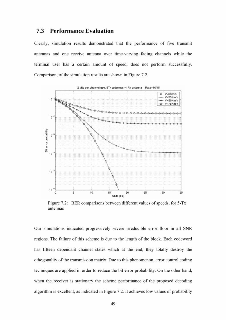
7.3 Performance Evaluation Clearly, simulation results demonstrated that the performance of five transmit

antennas and one receive antenna over time-varying fading channels while the

terminal user has a certain amount of speed, does not perform successfully.

Comparison, of the simulation results are shown in Figure 7.2.

Figure 7.2: BER comparisons between different values of speeds, for 5-Tx antennas

Our simulations indicated progressively severe irreducible error floor in all SNR

regions. The failure of this scheme is due to the length of the block. Each codeword

has fifteen dependant channel states which at the end, they totally destroy the

othogonality of the transmission matrix. Due to this phenomenon, error control coding

techniques are applied in order to reduce the bit error probability. On the other hand,

when the receiver is stationary the scheme performance of the proposed decoding

algorithm is excellent, as indicated in Figure 7.2. It achieves low values of probability

50

errors with low amount of signal-to-noise ratio. This scheme can successfully find

many applications where the receiver terminal is stationary, such as indoor wireless

networks.

51

Chapter 8

Conclusions Through our work, we investigated and demonstrated that significant gains can be

achieved by increasing the number of transmit antennas. We provided a special family

of complex orthogonal space-time codes for transmission using multiple transmit

antennas. The encoding and decoding of these codes have low complexity. Earlier

works have ignored the variation of the channel state over the length of the codeword.

This thesis presented performance results where the channel state varies from symbol

to symbol. For comparison and readability purposes we plot all the corresponding

BER curves for each number of transmit antennas, according to terminal speed, as

shown in the Figure 8.1.

Figure 8.1(a), shows bit error probability curves for different amount of transmit

antennas, where the receiver is stationary. It can been seen from the Figure 8.1(a), that

at bit error rates equal to 610− , the scheme with five transmit antennas achieves more

than 2-dB gain over the scheme with four transmit antennas. Moreover, the

performance of four transmit antennas achieve 5-dB gain over the three transmit

antennas and lastly the three transmit antennas more than 5-dB gain over the two

transmit antennas. Previous works confirm our results [11, 22, 24]. A possible

application of the scheme is to provide diversity improvement in all stationary receive

units in a wireless system, such as an indoor wireless network.

Figure 8.1(b), shows bit error probability curves for different amount of transmit

antennas, where the receiver have speed of 25h

km . Clearly, the following simulations

demonstrate that significant gains can be achieved by increasing the number of

transmit antennas.

52

Figure 8.1: Bit error probability versus SNR for different number of transmit antennas

(c) 50 km/h (d) 75 km/h

(e) 150 km/h

(b) 25 km/h (a) 0 km/h

53

It’s essential to observe that the two, three, and four transmit antennas schemes shows

no error floor at any value of SNR. However, when it comes for the scheme of five

transmit antennas under the speed of 25h

km , an error floor appears at high SNR

regions. This happens due the channel variations between the transmitted symbols and

due to the long length of the codeword. In addition, Figure 8.1(c), shows the

performance results of the abovementioned schemes under the speed of 50h

km ,

where the three transmit antennas can achieve better diversity gain (3-dB) than two

transmit antennas. However, four and five transmit antennas schemes appear to suffer

from error floor. In Figure 8.1(d), shows that all the schemes except from the two

transmit antenna scheme suffer from error floor at the high SNR regions under the

speed of 75h

km . Lastly, the performance results of two and three transmits antennas

schemes under the vehicle speed of 150h

km are demonstrated in Figure 8.1(e).

Future studies can consider combination of multiple transmit antennas and error

control coding techniques in order to suppress the above error floors.

54

Bibliography

[1] G. J. Foschini, "Layered space-time architecture for wireless communication in fading environment when using multi-element antennas," Bell Labs Tech. J., vol. 1, No. 2, pp. 41-59, 1996.

[2] G. J. Foschini and M. J. Gans, "On limitis of wireless communications in

fading environment when using multiple antennas," Wireless Personal Commun., pp. 311-355, 1998.

[3] T. L. Marzetta and B. M. Hochwald, "Capacity of a mobile multiple-antenna

communiction link in Rayleigh flat fading " IEEE Trans. Inform. Theory, vol. 45, pp. 139-157, Jan. 1999.

[4] I. E. Telatar, "Capacity of multi-antenna Gaussian channels," AT&T Bell Labs,

Internal Tech. Memo, 1995. See also, European Trans. Telecommun., vol. 10, no. 6, pp. 585-595, 1999.

[5] L. Zheng and D. N. C. Tse, "Communication on the Grassmann manifold: A

geometric approach to the noncoherent multiple-antenna channel," IEEE Trans. Inform. Theory, vol. 48, pp. 359-383, Feb. 2002.

[6] V. Tarokh, N. Seshadri, and A. R. Calderbank, "Space-time codes for high

data rate wireless communications: Performance criterion and code construction," IEEE Trans. Inform. Theory, vol. 44, pp. 744-765, Mar. 1998.

[7] V. Tarokh, H. Jafarkhani, and A. R. Calderbank, "Space-time block codes

from orthogonal designs," IEEE Trans. Inform. Theory, vol. 45, pp. 1456-1467, July 1999.

[8] B. M. Hochwald and T. L. Marzetta, "Unitary space-time modulation for

multiple-antenna communication in Rayleigh flat fading," IEEE Trans. Inform. Theory, vol. 46, pp. 543-564, Mar. 2000.

[9] A. Shokrollahi, B. Hassibi, B. M. Hochwald, and W. Sweldens,

"Representation theory for high-rate multiple-antenna code design," IEEE Trans. Commun., vol. 47, pp. 2335-2367, Sept. 2001.

[10] S. M. Alamouti, "A simple trasmit diversity technique for wireless

communications," IEEE J. Select. Areas Commun. , vol. 16, pp. 1451-1458, Oct. 1998.

[11] V. Tarokh, H. Jafarkhani, and A. R. Calderbank, "Space-Time Block Coding

for Wireless Communications: Performance Results," IEEE J. Select. Areas Commun., vol. 17, No.3, pp. 451-460, March 1999.

[12] X. B. Liang, "Orthogonal Designs with Maximal Rates," IEEE Trans. Inform.

Theory, vol. 49, pp. 2468-2503, Oct. 2003.

55

[13] R. Ludwing and P. Bretchko, RF Circuit Design Theory and Applications. New Jersey: Prendice-Hall, Inc., 2000.

[14] "http://www.iec.org/online/tutorials/smart_ant/index.html." [15] P. Tipler, Physics for Scientists and Engineers, 3 ed: Worth Publishers, 1991. [16] D. Gesbert, D. Shiu, P. J. Smith, and A. Naguib, "From theory to practice: An

Overview of MIMO Space–Time Coded Wireless Systems," IEEE J. Select. Areas Commun., vol. 21, No. 3, pp. 281-302, April 2003.

[17] W. C. Jakes, Microwave Mobile Communication. New York, NY: Wiley,

1974. [18] "http://mathworld.wolfram.com/." [19] "http://www.mathworks.com/access/helpdesk/help/techdoc/matlab.html." [20] "Digital Cellural Telecommmunications System (Phase 2+);Enhanced Data

rates for GSM Evolution (EDGE); European Telecommunications Standards Istitute. [Online] http:// www.etsi.org ".

[21] J. F. Adams, P. D. Lax, and R. S. Philips, "On matrices whose real linear

combinations are nonsingular," Proc. Amer. Math. Soc., vol. 16, pp. 318-322, 1965.

[22] F.-C. Zheng and A. G. Burr, "Receiver Design for Orthogonal Space-Time

Block Coding for Four Transmit Antennas over Time Selective-Fading Channels," in Proc. IEEE Globecom. San Francisco, CA, 2003, pp. 128-132.

[23] Z. Liu, X. Ma, and G. B. Giannakis, "Space-Time Coding and Kalman

Filtering for Time-Selective Fading Channels," IEEE Trans. Commun., vol. 50, No. 2, pp. 183-186, Feb. 2002.

[24] X. B. Liang, "A High-Rate Orthogonal Space-Time Block Code," IEEE

Communications Letters, vol. 7, pp. 222-223, May 2003.

56

Vita Ioannis D. Erotokritou was born in Nicosia, Cyprus, on August 3rd, 1979. In the

months after completing his high school education from Acropolis Lyceum in July of

1997, he enrolled as a student in the Higher Technical Institute in Cyprus, with focus

in electrical engineering. After completing his first degree in electrical engineering, in

June 2000, he joined the Greek Army and the Cyprus National Guard where he served

as an officer during his 26 month term. After he was discharged from the army in

2002, he enrolled in the Department of Electrical and Computer Engineering at

Louisiana State University where he graduated with a first class in spring 2004 with a

Bachelor of Science in Electrical Engineering. Upon graduation, Ioannis was accepted

as a graduate student in the same department and he is expected to get his Master of

Science in Electrical Engineering with specialization in telecommunications and

networking in spring 2006.