Space-Time Block Coding for Multiple Antenna Systems · PDF fileSpace-Time Block Coding for...
127
DISSERTATION Space-Time Block Coding for Multiple Antenna Systems ausgef¨ uhrt zum Zwecke der Erlangung des akademischen Grades eines Doktors der technischen Wissenschaften eingereicht an der Technischen Universit¨ at Wien Fakult¨ at f¨ ur Elektrotechnik und Informationstechnik von Dipl.-Ing. Biljana Badic Wien, November 2005
Transcript of Space-Time Block Coding for Multiple Antenna Systems · PDF fileSpace-Time Block Coding for...
DISSERTATION
Space-Time Block Codingfor
Multiple Antenna Systems
ausgefuhrt zum Zwecke der Erlangung des akademischen Gradeseines Doktors der technischen Wissenschaften
eingereicht an der Technischen Universitat WienFakultat fur Elektrotechnik und Informationstechnik
von
Dipl.-Ing. Biljana Badic
Wien, November 2005

unter der Leitung von
Univ. Prof. Dr. Johann Weinrichter
Institut fur Nachrichten- und HochfrequenztechnikTechnischen Universitat Wien
Fakultat fur Elektrotechnik und Informationstechnik
Univ. Prof. Dr. Markus Rupp
Institut fur Nachrichten- und HochfrequenztechnikTechnischen Universitat Wien
Fakultat fur Elektrotechnik und Informationstechnik


”Anyone who stops learning is old, whether at twenty or eighty.Anyone who keeps learning stays young. The greatest thing inlife is to keep your mind young.”
Henry Ford


Acknowledgement
It is my pleasure to thank the people with whom I enjoyed discussing problems and sharing ideas. I amespecially thankful to Prof. Dr. Weinrichter, for his valuable reading of the thesis, for having discussionstogether line by line, and giving me inestimable feedback.I also wish to thank Prof. Dr. Rupp for his encouragement, forreading the thesis and for providing mecontinuously support for my PhD work.I am deeply thankful to all my colleagues who contributed to different subjects of this thesis.And, my final thank is for my family, their love and support through my work.
i

Abstract
The demand for mobile communication systems with high data rates has dramatically increased in recentyears. New methods are necessary in order to satisfy this huge communications demand, exploiting thelimited resources such as bandwidth and power as efficient aspossible. MIMO systems with multiple an-tenna elements at both link ends are an efficient solution forfuture wireless communications systems asthey provide high data rates by exploiting the spatial domain under the constraints of limited bandwidthand transmit power. Space-Time Block Coding (STBC) is a MIMOtransmit strategy which exploitstransmit diversity and high reliability. STBCs can be divided into two main classes, namely, OrthogonalSpace-Time Block Codes (OSTBCs) and Non-Orthogonal Space-Time Block Codes (NOSTBCs). TheQuasi-Orthogonal Space-Time Block Codes (QSTBCs) belong to class of NOSTBCs and have been anintensive area of research. The OSTBCs achieve full diversity with low decoding complexity, but atthe price of some loss in data rate. Full data rate is achievable in connection with full diversity only inthe case of two transmit antennas in case of complex-valued symbol transmission. For more than twotransmit antennas full data rate can be achieved with QSTBCswith a small loss of the diversity gain.However, it has been shown that QSTBCs perform even better than OSTBCs in the SNR range of prac-tical interest (up to 20 dB) that makes this class of STBCs an attractive area of research.
The main goal of this work is to provide a unified theory of QSTBCs for four transmit antennas andone (or more) receive antennas. The thesis consists of two main parts: In the first part we analyze theQSTBCs transmission without any channel knowledge at the transmitter and in the second part we an-alyze transmission with QSTBCs assuming partial channel state (CSI) information at the transmitter.For both cases, the QSTBCs are studied on spatially correlated and uncorrelated frequency flat MIMOchannels applying a Maximum Likelihood receivers as well asa low complexity linear Zero-Forcingreceivers. The spatial correlation is modelled by the so-called Kronecker Model. Measured indoor chan-nels are also used in our simulations to show the performanceof the QSTBCs in real-world environment.
In the first part of this thesis we give a consistent definitionof QSTBCs for four transmit antennas.We show that different QSTBCs are obtained by linear transformations and that already known codescan be transformed into each other. We show that the (4 × 1) MIMO channel in the case of applyingquasi-orthogonal codes can be transformed into an equivalent highly structured virtual (4 × 4) MIMOchannel matrix. The structure of the equivalent channel is of vital importance for the performance of theQSTBCs. We show that the off-diagonal elements of the virtual channel matrix are responsible for somesignal self-interference at the receiver. The closer theseoff-diagonal elements of the virtual channel ma-trix are to zero, the closer is the code to an orthogonal code.Based on this self-interference parameter itcan be shown that only 12 QSTBC types with different performance exist.
In the second part of the thesis we provide two simple methodsto improve the QSTBC transmis-sion when partial CSI is available at the transmitter. We propose two novel closed-loop transmissionschemes, namely channel adaptive code selection (CACS) andchannel adaptive transmit antenna selec-tion (CAAS). By properly utilization of partial CSI at the transmitter, we show that QSTBCs can achievefull diversity and nearly strict orthogonality with a smallamount of feedback bits returned from the re-ceiver back to the transmitter. CACS is very simple and requires only a small amount of the feedbackbits. With CAAS full diversity of four and a small improvement of the outage capacity can be achieved.The CAAS increases the channel capacity substantially, butthe required number of the feedback bitsincreases exponentially with the number of available transmit antennas.
iii

Zusammenfassung
Die Nachfrage nach Mobilfunksystemen mit hoher Datenrate undUbertragungsqualitat ist in den letztenJahren dramatisch gestiegen. Zur Deckung des hohen Kommunikationsbedarfs werden neue Technolo-gien benotigt, welche die knappen Ressourcen, wie Bandbreite und Sendeleistung, optimal ausnutzenkonnen. MIMO Systeme, bestehend aus mehreren Sende- und Empfangsantennen, stellen eine ef-fiziente Maßnahme fur eine deutliche Steigerung derUbertragungskapazitat gegenuber konventionellenKommunikationssystemen (mit je einer Sende- und Empfangsantenne) bei gleicher Sendeleistung undUbertragungsbandbreite dar. Die Raum-Zeit Block Codierung (STBC) ist einUbertragunsverfahren,das neben der zeitlichen und der spektralen auch die raumliche Dimension derUbertragungsstreckeausnutzt. Man unterscheidet zwischen orthogonalen Raum-Zeit Block Codes (OSTBCs) und nicht-orthogonalen Raum-Zeit Block Codes (NOSTBCs). Die quasi-orthogonalen Raum-Zeit Block Codes(QSTBCs) sind eine Unterklasse der NOSTBCs. OSTBCs erreichen volle Diversitat mit einem ein-fachen Decodierungsalgorithmus, jedoch mit einer eingeschrankten Datenrate. Volle Datenrate und volleDiversitat sind gleichzeitig nur in MIMO Systemen mit zweiSendeantennen erreichbar. In MIMO Syste-men mit mehr als zwei Sendeantennen kann man volle Datenratenur mittels QSTBCs erreichen, welcheaber einen Diversitatsverlust zur Folge haben. Es wurde festgestellt, dass im SNR Bereich bis zu 20 dBQSTBCs sogar weniger Fehler anfallig sind als OSTBCs. Aus diesem Grund sind QSTBCs ein wichtigesForschungsgebiet geworden.
Das Ziel dieser Arbeit ist die Formulierung einer vereinheitlichten Theorie uber QSTBCs fur vier Sendean-tennen und eine (oder mehrere) Empfangsantennen. Die Arbeit umfasst zwei Themenschwerpunkte: Imersten Teil, analysieren wir die QSTBC-Ubertragung ohne Kanalkenntnis am Sender und im zweitenTeil analysieren wir Leistungsvermogen von QSTBCs unter der Annahme, dass der Sender den Kanalnur teilweise kennt. In beiden Fallen werden QSTBCs uber raumlich korrelierte und raumlich unkorre-lierte echofreie Funkkanale unter der Verwendung von Maximum-Likelihood Empfangern sowie auchunter Verwendung von einfachen Zero-Forcing Empfangern untersucht. Die raumliche Korrelation wirdmit dem so genannten Kronecker Modell eingebracht. Um zu zeigen, wie sich QSTBCs in realen MIMOKanalen verhalten, haben wir in unseren Simulationen Messungen aus einem Buroraum-Szenario ver-wendet.
Im ersten Teil dieser Dissertation definieren wir QSTBCs fur vier Sendeantennen. Wir zeigen, dassverschiedene QSTBCs durch lineare Transformationen konstruiert werden konnen und dass die bereitsbestehenden Codes ineinander uberfuhrt werden konnen.Im Falle von QSTBCs wird in dieser Arbeitgezeigt, dass der(4 × 1) MIMO-Kanal in einen aquivalenten, hoch-struktuierten, virtuellen (4 × 4)MIMO-Kanal transformiert werden kann. Die Struktur des aquivalenten Kanals ist von zentraler Be-deutung fur Eigenschaften von QSTBCs. Die Elemente, welche sich nicht auf der Hauptdiagonale dervirtuellen Kanalmatrix befinden, konnen als kanalabhangiger SelbstinterferenzparameterX interpretiertwerden. Wir zeigen, dassX eine bedeutende Wirkung auf die Systemeigenschaften hat. Je kleinerXist, um so naher ist der Code einem orthogonalen Code. Basierend auf dem ParameterX, wird gezeigt,dass es nur 12 verschiedenen Typen von QSTBCs gibt.
Im zweiten Teil dieser Dissertation schlagen wir zwei einfache Methoden vor, um das Leistungsvermogenvon QSTBCs zu verbessern. Unter der Annahme, dass der Senderden Kanal nur teilweise kennt,schlagen wir eine kanaladaptive Codeselektion (CACS) und eine kanaladaptive Sendeantennenselek-tion (CAAS) vor. Bei richtiger Anwendung der partiellen Kanalkenntnis am Sender, zeigen wir, dass
v
QSTBCs volle Diversitat und beinahe volle Orthogonalitat erreichen konnen. Dabei wird nur wenigKanalinformation vom Empfanger zum Sender gesendet. Die CACS ist sehr einfach und braucht nur1-2 Ruckkopplungsbits pro Schwundblock um die volle Diversitat vier zu erreichen. Leider erhoht sichbei diesem Verfahren die Kanalkapazitat nicht wesentlich. Dem gegenuber erhoht sich die Kanalka-pazitat bei Verwendung der CAAS betrachtlich! Die Anzahldie notigen Ruckkopplungsbits steigt aberexponentiell mit der Anzahl der vorhandenen Sendeantennen.
Contents
1 Introduction 1
1.1 Outline of the Thesis . . . . . . . . . . . . . . . . . . . . . . . . . . . . . .. . . . . . 2
2 Multiple-Antenna Wireless Communication Systems 5
2.1 Introduction . . . . . . . . . . . . . . . . . . . . . . . . . . . . . . . . . . . .. . . . . 5
2.1.1 Multi - Antenna Transmission Methods . . . . . . . . . . . . . .. . . . . . . . 7
2.2 Modelling the Wireless MIMO System . . . . . . . . . . . . . . . . . .. . . . . . . . . 8
2.2.1 System (and Channel) Model . . . . . . . . . . . . . . . . . . . . . . .. . . . . 8
2.2.2 Channel Model . . . . . . . . . . . . . . . . . . . . . . . . . . . . . . . . . .. 9
2.2.2.1 Spatially Uncorrelated Channel . . . . . . . . . . . . . . . .. . . . . 9
2.2.2.2 Spatially Correlated Channel . . . . . . . . . . . . . . . . . .. . . . 9
2.2.2.3 Noise Term and SNR-Definition . . . . . . . . . . . . . . . . . . .. 11
2.3 Channel Capacity . . . . . . . . . . . . . . . . . . . . . . . . . . . . . . . . .. . . . . 12
2.4 Summary . . . . . . . . . . . . . . . . . . . . . . . . . . . . . . . . . . . . . . . . .. 13
3 Space-Time Coding 15
3.1 Introduction . . . . . . . . . . . . . . . . . . . . . . . . . . . . . . . . . . . .. . . . . 15
3.2 Space-Time Coded Systems . . . . . . . . . . . . . . . . . . . . . . . . . .. . . . . . 15
3.2.1 Performance Analysis . . . . . . . . . . . . . . . . . . . . . . . . . . .. . . . 16
3.2.1.1 Error Probability for Slow Fading Channels . . . . . . .. . . . . . . 17
3.2.1.2 Error Probability for Fast Fading Channels . . . . . . .. . . . . . . . 18
3.2.2 Space-Time Codes . . . . . . . . . . . . . . . . . . . . . . . . . . . . . . .. . 20
3.3 Space-Time Block Codes . . . . . . . . . . . . . . . . . . . . . . . . . . . .. . . . . . 20
3.3.1 Alamouti Code . . . . . . . . . . . . . . . . . . . . . . . . . . . . . . . . . .. 21
3.3.2 Equivalent Virtual(2 × 2) Channel Matrix (EVCM) of the Alamouti Code . . . 22
3.3.3 Linear Signal Combining and Maximum Likelihood Decoding of the AlamoutiCode . . . . . . . . . . . . . . . . . . . . . . . . . . . . . . . . . . . . . . . . 23
3.3.4 Orthogonal Space-Time Block Codes (OSTBCs) . . . . . . . .. . . . . . . . . 24
vii
viii CONTENTS
3.3.4.1 Examples of OSTBCs . . . . . . . . . . . . . . . . . . . . . . . . . . 25
3.3.4.2 Bit Error Rate (BER) of OSTBCs . . . . . . . . . . . . . . . . . . .. 26
3.3.5 Quasi-Orthogonal Space-Time Block Codes (QSTBC) . . .. . . . . . . . . . . 28
3.4 Summary . . . . . . . . . . . . . . . . . . . . . . . . . . . . . . . . . . . . . . . . .. 29
4 Quasi-Orthogonal Space-Time Block Code Design 31
4.1 Introduction . . . . . . . . . . . . . . . . . . . . . . . . . . . . . . . . . . . .. . . . . 31
4.2 Structure of QSTBCs . . . . . . . . . . . . . . . . . . . . . . . . . . . . . . .. . . . . 31
4.3 Known QSTBCs . . . . . . . . . . . . . . . . . . . . . . . . . . . . . . . . . . . . .. 32
4.3.1 Jafarkhani Quasi-Orthogonal Space-Time Block Code .. . . . . . . . . . . . . 32
4.3.2 ABBA Quasi-Orthogonal Space-Time Block Code . . . . . . .. . . . . . . . . 34
4.3.3 Quasi-Orthogonal Space-Time Block Code Proposed by Papadias and Foschini . 34
4.4 New QSTBCs . . . . . . . . . . . . . . . . . . . . . . . . . . . . . . . . . . . . . . .. 36
4.4.1 New QSTBCs Obtained by Linear Transformations . . . . . .. . . . . . . . . . 36
4.5 Equivalent Virtual Channel Matrix (EVCM) . . . . . . . . . . . .. . . . . . . . . . . . 39
4.6 Receiver Algorithms for QSTBCs . . . . . . . . . . . . . . . . . . . . .. . . . . . . . 40
4.6.1 Maximum Ratio Combining . . . . . . . . . . . . . . . . . . . . . . . . .. . . 40
4.6.2 Maximum Likelihood (ML) Receiver . . . . . . . . . . . . . . . . .. . . . . . 41
4.6.3 Linear Receivers . . . . . . . . . . . . . . . . . . . . . . . . . . . . . . .. . . 42
4.7 EVCMs for known QSTBCs . . . . . . . . . . . . . . . . . . . . . . . . . . . . .. . . 44
4.7.1 EVCM for the Jafarkhani Code . . . . . . . . . . . . . . . . . . . . . .. . . . 45
4.7.2 EVCM for the ABBA Code . . . . . . . . . . . . . . . . . . . . . . . . . . . .45
4.7.3 EVCM for the Papadias-Foschini Code . . . . . . . . . . . . . . .. . . . . . . 46
4.7.4 Other EVCMs with Channel Independent Diagonalization of G . . . . . . . . . 46
4.7.5 Statistical Properties of the Channel Dependent Self-Interference Parameter . . . 47
4.7.6 Common Properties of the Equivalent Virtual Channel Matrices Correspondingto QSTBCs . . . . . . . . . . . . . . . . . . . . . . . . . . . . . . . . . . . . . 49
4.7.7 Useful QSTBC Types . . . . . . . . . . . . . . . . . . . . . . . . . . . . . .. 49
4.7.7.1 QSTBCs with real and purely imaginary-valued self-interference pa-rameters . . . . . . . . . . . . . . . . . . . . . . . . . . . . . . . . . 50
4.7.8 Impact of Spatially Correlated Channels on the Self-Interference Parameter X . . 52
4.8 BER Performance of 12 useful QSTBCs . . . . . . . . . . . . . . . . . .. . . . . . . . 53
4.8.1 BER Performance of QSTBCs using Linear ZF Receiver . . .. . . . . . . . . . 53
4.8.2 BER Performance of QSTBCs using a ML Receiver . . . . . . . .. . . . . . . 54
4.8.3 BER Performance of QSTBCs on Measured MIMO Channels . .. . . . . . . . 55
4.8.3.1 Measurement Setup . . . . . . . . . . . . . . . . . . . . . . . . . . . 55
4.8.3.2 Simulation Results . . . . . . . . . . . . . . . . . . . . . . . . . . .. 57
4.9 Summary . . . . . . . . . . . . . . . . . . . . . . . . . . . . . . . . . . . . . . . . .. 58
CONTENTS ix
5 Performance of QSTBCs with Partial Channel Knowledge 59
5.1 Introduction . . . . . . . . . . . . . . . . . . . . . . . . . . . . . . . . . . . .. . . . . 59
5.1.1 QSTBCs Exploiting Partial CSI using Limited Feedback. . . . . . . . . . . . . 60
5.2 Channel Adaptive Code Selection (CACS) . . . . . . . . . . . . . .. . . . . . . . . . . 61
5.2.1 CACS with One Feedback Bit per Code Block . . . . . . . . . . . .. . . . . . 61
5.2.2 Probability Distribution of the Resulting Interference Parameter W . . . . . . . . 64
5.2.3 CACS with Two Control Bits fed back from the Receiver tothe Transmitter . . . 64
5.2.4 Probability Distribution of the Interference Parameter Z . . . . . . . . . . . . . 65
5.2.5 Simulation Results . . . . . . . . . . . . . . . . . . . . . . . . . . . . .. . . . 66
5.2.5.1 Spatially Uncorrelated MIMO Channels . . . . . . . . . . .. . . . . 66
5.2.5.2 Spatially Correlated MIMO Channels . . . . . . . . . . . . .. . . . . 66
5.2.5.3 Measured Indoor MIMO Channels . . . . . . . . . . . . . . . . . .. 73
5.2.5.4 Real-Time Evaluation . . . . . . . . . . . . . . . . . . . . . . . . .. 74
5.3 Channel Adaptive Transmit Antenna Selection (CAAS) . . .. . . . . . . . . . . . . . . 77
5.3.1 Transmission Scheme . . . . . . . . . . . . . . . . . . . . . . . . . . . .. . . 78
5.3.2 Antenna Selection Criteria . . . . . . . . . . . . . . . . . . . . . .. . . . . . . 79
5.3.3 Simulation Results . . . . . . . . . . . . . . . . . . . . . . . . . . . . .. . . . 81
5.3.4 Is there a Need for QSTBCs with Antenna Selection? . . . .. . . . . . . . . . . 85
5.3.5 Code and Antenna Selection . . . . . . . . . . . . . . . . . . . . . . .. . . . . 86
5.4 Channel Capacity of QSTBCs . . . . . . . . . . . . . . . . . . . . . . . . .. . . . . . 88
5.4.1 Capacity of Orthogonal STBC vs. MIMO Channel Capacity. . . . . . . . . . . 88
5.4.2 Capacity of QSTBCs with No Channel State Information at the Transmitter . . . 90
5.4.3 Capacity of QSTBCs with Channel State Information at the Transmitter . . . . . 91
5.4.4 Simulation Results . . . . . . . . . . . . . . . . . . . . . . . . . . . . .. . . . 91
5.5 Summary . . . . . . . . . . . . . . . . . . . . . . . . . . . . . . . . . . . . . . . . .. 93
6 Conclusions 95
Appendices 97
A Alamouti-type STBCs for Two Transmit Antennas 98
B ”Useful” QSTBC Matrices for Four Transmit Antennas 99
C Maximum Likelihood Receiver Algorithms 101
D Acronyms 102

List of Figures
2.1 MIMO model withnt transmit antennas andnr receive antennas. . . . . . . . . . . . . . 8
2.2 Ergodic MIMO channel capacity vs. SISO channel capacity(spatially uncorrelated chan-nel). . . . . . . . . . . . . . . . . . . . . . . . . . . . . . . . . . . . . . . . . . . . . . 13
3.1 A block diagram of the Alamouti space-time encoder. . . . .. . . . . . . . . . . . . . . 21
3.2 The BER performance of the QPSK Alamouti Scheme,nt = 2, nr = 1,2. . . . . . . . . 24
3.3 Bit error performance for OSTBC of 3 bits/channel use onnt × 1 channels with i.i.dRayleigh fading channel coefficients. . . . . . . . . . . . . . . . . . .. . . . . . . . . . 27
3.4 Bit error performance for OSTBC of 2 bits/channel use onnt × 1 channels with i.i.dRayleigh fading channel coefficients. . . . . . . . . . . . . . . . . . .. . . . . . . . . . 27
3.5 Comparison of OSTBCs and QSTBC on ant × 1 channel withnt = 4 and i.i.d Rayleighfading channel coefficients transmitting 2 bits/channel use. . . . . . . . . . . . . . . . . 28
4.1 Comparison of known code designs on spatially uncorrelated and spatially correlatedMIMO channels (ρ = 0,95) with ML receiver. . . . . . . . . . . . . . . . . . . . . . . . 35
4.2 The performance of the QSTBC compared with ideal three and four-path diversity. . . . 44
4.3 The pdf of|XEA|. . . . . . . . . . . . . . . . . . . . . . . . . . . . . . . . . . . . . . . 48
4.4 Expectation of|Xi| as a function ofρ. . . . . . . . . . . . . . . . . . . . . . . . . . . . 53
4.5 BER performance of QSTBCsS1 −S6 on spatially uncorrelated and spatially correlatedchannels using a ZF receiver a)ρ = 0,75, b) ρ = 0,95. . . . . . . . . . . . . . . . . . . 54
4.6 BER performance of QSTBCsS7−S12 on spatially uncorrelated and spatially correlatedchannels and ZF receiver a)ρ = 0,75, b) ρ = 0,95. . . . . . . . . . . . . . . . . . . . . 54
4.7 BER performance of QSTBCsS1 −S6 on spatially uncorrelated and spatially correlatedchannels and ML receiver a)ρ = 0,75, b) ρ = 0,95. . . . . . . . . . . . . . . . . . . . . 55
4.8 BER performance of QSTBCsS7−S12 on spatially uncorrelated and spatially correlatedchannels and ML receiver a)ρ = 0,75, b) ρ = 0,95. . . . . . . . . . . . . . . . . . . . . 56
4.9 BER performance of QSTBCsS1 to S12 on real MIMO channels and ZF receiver a)QSTBCs with real-valued ofXi , b) QSTBCs with imaginary-valued ofXi. . . . . . . . 57
4.10 BER performance of QSTBCsS1 to S12 on real MIMO channels and ML receiver a)QSTBCs with real-valued ofXi , b) QSTBCs with imaginary-valued ofXi. . . . . . . . 58
5.1 Closed-loop scheme with code selection,nt = 4, nr = 1. . . . . . . . . . . . . . . . . . 62
xi
xii LIST OF FIGURES
5.2 One sided pdf of the interference parametersX,W , andZ. . . . . . . . . . . . . . . . . 66
5.3 BER for a (4× 1) closed-loop scheme applying a ZF receiver, uncorrelated MISO channel. 67
5.4 BER for (4 × 1) closed-loop scheme applying a ML receiver, uncorrelated MISO channel. 67
5.5 BER of (4× 1) closed-loop scheme with one bit feedback, ZF receiver and fading corre-lation factorρ. . . . . . . . . . . . . . . . . . . . . . . . . . . . . . . . . . . . . . . . . 68
5.6 BER of (4 × 1) closed-loop scheme with two bits feedback, ZF receiver andfadingcorrelation factorρ. . . . . . . . . . . . . . . . . . . . . . . . . . . . . . . . . . . . . . 68
5.7 BER of (4 × 1) closed-loop scheme with one bit feedback, ML receiver and fading cor-relation factorρ. . . . . . . . . . . . . . . . . . . . . . . . . . . . . . . . . . . . . . . . 69
5.8 BER of (4 × 1) closed-loop scheme with two bits feedback, ML receiver andfadingcorrelation factorρ. . . . . . . . . . . . . . . . . . . . . . . . . . . . . . . . . . . . . . 69
5.9 BER-Performance comparison of the ABBA- and EA-type QSTBC for spatially uncor-related channels, ZF receiver. . . . . . . . . . . . . . . . . . . . . . . . .. . . . . . . . 71
5.10 BER-Performance comparison of the ABBA- and EA-type QSTBC for spatially corre-lated channels withρ = 0,5, ZF receiver. . . . . . . . . . . . . . . . . . . . . . . . . . . 71
5.11 Comparison of the BER-Performance between the ABBA- and EA-type QSTBC for spa-tially correlated channels withρ = 0,75, ZF receiver. . . . . . . . . . . . . . . . . . . . 72
5.12 Comparison of the BER-Performance between the ABBA- and EA-type QSTBC for spa-tially correlated channels withρ = 0,95, ZF receiver. . . . . . . . . . . . . . . . . . . . 72
5.13 One sided pdf ofX for correlated channels for a) the EA-type QSTBC, b) the ABBA-type QSTBC. . . . . . . . . . . . . . . . . . . . . . . . . . . . . . . . . . . . . . . . . 73
5.14 Performance of code selection on measured channels, Scenario A (NLOS) and ZF receiver. 74
5.15 Performance of code selection on measured channels, Scenario A (NLOS) and ML receiver. 75
5.16 Performance of code selection on measured channels, Scenario B (LOS) and ZF receiver. 75
5.17 Performance of code selection on measured channels, Scenario B (LOS) and ML receiver. 76
5.18 BER-performance of code selection in real-time measurement. . . . . . . . . . . . . . . 76
5.19 Antenna Selection at the Transmitter,h = [h1, h2, · · · , hNt ] → hsel = [hi, hj , hk, hl]. . 78
5.20 Comparison of the three antenna selection criteria forselectingnt = 4 out of Nt = 6available antennas with i.i.d. Rayleigh fading channel coefficients. . . . . . . . . . . . . 80
5.21 One sided pdf of|X| for three selection criteria,nt = 4 out ofNt = 6, Nr = nr = 1. . . 81
5.22 Transmit antenna selection, channels with i.i.d. Rayleigh channel coefficients,nt = 4out of5 ≤ Nt ≤ 7. . . . . . . . . . . . . . . . . . . . . . . . . . . . . . . . . . . . . . 82
5.23 Transmit selection performance forNt = 5,6,7 using the maxh2(1 − X2) criterioncompared with the corresponding ideal transmit diversity systems. . . . . . . . . . . . . 83
5.24 Interrelation of closed loop transmit selection gain on i.i.d. channels and required amountof feedback information at BER=10−4. . . . . . . . . . . . . . . . . . . . . . . . . . . . 83
5.25 Transmit antenna selection on spatially correlated channels, (ρ = 0,95). . . . . . . . . . 84
5.26 Transmit antenna selection on measured MIMO channels,Scenario A (NLOS), ZF receiver. 84
5.27 Transmit antenna selection on measured MIMO channels,Scenario B (LOS), ZF receiver. 85
LIST OF FIGURES xiii
5.28 Transmit antenna selection performance for three transmission schemes. . . . . . . . . . 86
5.29 Transmit antenna selection performance when a bit error ratio of BERfeedback = 10−2
at the feedback link is assumed. . . . . . . . . . . . . . . . . . . . . . . . .. . . . . . 87
5.30 Joint antenna/code selection,nt = 4 out of5 ≤ Nt ≤ 7. . . . . . . . . . . . . . . . . . . 88
5.31 One sided pdfs ofX for joint antenna/code selection,Nt = 6. . . . . . . . . . . . . . . 89
5.32 3% outage capacity of QSTBCs with code selection when comparedwith ideal open-looptransmission scheme,nt = 4, nr = 1. . . . . . . . . . . . . . . . . . . . . . . . . . . . 92
5.33 3% outage capacity of QSTBCs with transmit antenna selection when compared with anideal open-loop transmission scheme,Nt = 5,6,7, nt = 4, nr = 1. . . . . . . . . . . . . 92
5.34 Comparison of the3% outage capacity for the QSTBC with CSI at the transmitter andaMISO system without any CSI at the transmitter. . . . . . . . . . . .. . . . . . . . . . 93

Chapter 1
Introduction
Communication technologies have become a very important part of human life. Wireless communicationsystems have opened new dimensions in communications. People can be reached at any time and at anyplace. Over 700 million people around the world subscribe toexisting second and third generationcellular systems supporting data rates of9,6 kbps to2 Mbps. More recently, IEEE 802.11 wireless LANnetworks enable communication at rates of around 54 Mbps andhave attracted more than1,6 billion USDin equipment sales. Over the next ten years, the capabilities of these technologies are expected to movetowards the 100 Mbps - 1 Gbps range and to subscriber numbers of over two billion. At the present time,the wireless communication research community and industry discuss standardizations for the fourthmobile generation (4G). The research community has generated a number of promising solutions forsignificant improvements in system performance. One of the most promising future technologies inmobile radio communications is multi antenna elements at the transmitter and at the receiver.
MIMO stands formultiple-input multiple-outputand means multiple antennas at both link ends ofa communication system, i.e., at the transmit and at the receive side. The multiple-antennas at thetransmitter and/or at the receiver in a wireless communication link open a new dimension in reliablecommunication, which can improve the system performance substantially. The idea behind MIMO is thatthe transmit antennas at one end and the receive antennas at the other end are ”connected and combined”in such a way that the quality (the bit error rate (BER), or thedata rate) for each user is improved.The core idea in MIMO transmission isspace-timesignal processing in which signal processing in timeis complemented by signal processing in the spatial dimension by using multiple, spatially distributedantennas at both link ends.
Because of the enormous capacity increase MIMO systems offer, such systems gained a lot of interestin mobile communication research [1], [2]. One essential problem of the wireless channel is fading,which occurs as the signal follows multiple paths between the transmit and the receive antennas. Undercertain, not uncommon conditions, the arriving signals will add up destructively, reducing the receivedpower to zero (or very near to zero). In this case no reliable communication is possible.Fading can be mitigated by diversity, which means that the information is transmitted not only once butseveral times, hoping that at least one of the replicas will not undergo severe fading. Diversity makes useof an important property of wireless MIMO channels: different signal paths can be often modeled as anumber of separate, independent fading channels. These channels can be distinct in frequency domainor in time domain.
Several transmission schemes have been proposed that utilize the MIMO channel in different ways,e.g., spatial multiplexing, space-time coding or beamforming. Space-time coding (STC), introduced firstby Tarokh at el. [3], is a promising method where the number ofthe transmitted code symbols per timeslot are equal to the number of transmit antennas. These codesymbols are generated by the space-time
1
2 1.1. OUTLINE OF THE THESIS
encoder in such a way that diversity gain, coding gain, as well as high spectral efficiency are achieved.
Space-time coding finds its application in cellular communications as well as in wireless local areanetworks. There are various coding methods as space-time trellis codes (STTC), space-time block codes(STBC), space-time turbo trellis codes and layered space-time (LST) codes. A main issue in all theseschemes is the exploitation of redundancy to achieve high reliability, high spectral efficiency and highperformance gain. The design of STC amounts to find code matrices that satisfy certain optimality crite-ria. In particular, STC schemes optimize a trade-off between the three conflicting goals of maintaining asimple decoding algorithm, obtaining low error probability, and maximizing the information rate.
In the last few years the research community has made an enormous effort to understand space-time codes, their performance and their limits. The purposeof this work is to explain the concept ofspace-time block coding in a systematic way. This thesis provides an overview of STBC design princi-ples and performance. The main focus is devoted to so-calledquasi-orthogonal space-time block codes(QSTBCs). Our goal is to provide a unified theory of QSTBCs forfour transmit antennas and one receiveantenna and to analyze their performance on different MIMO channels, with and without channel stateinformation (CSI) available at the transmitter.
1.1 Outline of the Thesis
This thesis consists of six chapters and three appendices and is organized as follows:
Chapter 2introduces MIMO systems. We describe multiple antenna systems and the correspondingstatistical parameters [1]-[15] . The potential of MIMO systems as well their problems are described. Wepresent two channel correlation models which will be used throughout this thesis [16]-[22]. The Signal-to-Noise Ratio (SNR) definition used in this thesis is explained in detail. At the end of this chapter, themost important parameter of a MIMO system, the channel capacity, is presented [1], [2].
Chapter 3deals with space-time coding techniques and their performance in slow and fast fadingMIMO channels. It provides a systematic discussion of STCs and sets the framework for the rest of thisthesis. We start with the performance and the design criteria of STCs defined in [3]. We provide a moresystematic discussion of space-time block coding (STBC). We first explain the Alamouti STBC [29] thatprovides a transmit diversity of two. Orthogonal and quasi-orthogonal designs [30] -[34] are presentedand their performance is evaluated by simulations.
Chapter 4is devoted to the analysis of quasi-orthogonal STBCs in open-loop transmission systems.The complete family of OSTBCs is well understood, but for QSTBCs only examples have been reportedin the literature [42]-[47] without systematic analysis and precise definition. E.g., in [48] the charactermatrices of known QSTBCs have been analyzed and new versionsof QSTBCs have been presented. In[49] the design of the receiver structure for the QSTBC proposed in [42] has been studied.The primary goal of this chapter is to provide a unified theoryof QSTBCs for four transmit antennasand one receive antenna. Our aim is to present the topic as consistent as possible. The chapter startswith an overview on known QSTBCs and their performance including recent analytic findings and theirexperimental validation [42]-[44]. We introduce a conceptof extending OSTBCs to QSTBCs and showhow families of codes with essentially identical code properties but different transmission properties inspatially correlated channels can be generated. No researcher ever dared to define exactly what a quasi
CHAPTER 1. INTRODUCTION 3
orthogonal code exactly is. The word quasi is not well definedin such context. We give a consistent def-inition of QSTBCs for four transmit antennas and show that essentially only 12 QSTBCs with differentperformance exits. We analyze the structuring property of the equivalent virtual MIMO channel matrix(EVCM) resulting from the QSTBCs due to which we can reformulate the transmission problem in anequivalent form much more suitable for the system performance analysis. Finally, we discuss the per-formance of various receivers under QSTBC transmission. ByMonte Carlo simulations we evaluate theBER performance of the 12 different QSTBCs on i.i.d. channels as well as on correlated and measuredindoor MIMO channels.The QSTBCs treated in this chapter do not exploit at least partial channel knowledge at the transmitter.However in some applications, the transmitter can exploit channel state information (CSI) to improve theoverall performance of the system, especially in case of spatially correlated channels [66], [67], [80].
Chapter 5provides very simple methods to improve the QSTBC transmission strategy when the trans-mitter knows the channel. Evaluating the performance of QSTBCs with feedback of CSI has been anintensive area of research resulting in various transmission strategies [64] - [67]. In these works (andreferences therein) it has been shown that partial channel knowledge can be advantageously exploited toadapt the transmission strategy in order to optimize the system performance. In this chapter we study twolow complexity closed-loop transmission schemes relying on partial CSI feedback showing that QSTBCscan achieve full diversity even if only a small amount of channel state information is available at thetransmitter. We present a simple version of a code selectionand a simple version of an antenna selectionmethod in combination with QSTBCs. In both cases the receiver returns a small amount of the CSI thatenables the transmitter to minimize the interference parameter resulting from the non-orthogonality ofall QSTBCs. In this way full diversity and nearly full-orthogonality can be achieved with a maximumlikelihood (ML) receiver as well as with a simple zero-forcing (ZF) receiver.
Chapter 6highlights the content of the thesis and summarises the major results.
Appendix Ashows 16 different(2× 2) Alamouti-like code matrices for two transmit antennas neces-sary for the design of QSTBCs in Chapter 4.Appendix Bpresents some examples of useful QSTBCs forfour transmit antennas explained in Section 4.7.7.Appendix Cexplains the principle of the maximum-likelihood detection algorithm discussed in Section 4.6.2. In Appendix D, in the thesis oftentimes used,acronyms are listed.

4 1.1. OUTLINE OF THE THESIS
Chapter 2
Multiple-Antenna WirelessCommunication Systems
2.1 Introduction
The invention of the radio telegraph byGuglielmo Marconimore than hundert years ago marks the com-mencement of wireless communications. In the last 20 years,the rapid progress in radio technology hasactivated a communications revolution. Wireless systems have been deployed through the world to helppeople and machines to communicate with each other independent of their location.”Always best con-nected”is one of the slogans for the fourth generation of wireless communications system (4G), meaningthat your wireless equipment should connect to the network or system that at the moment is the ”best”for you.Wireless communication is highly challenging due to the complex, time varying propagation medium. Ifwe consider a wireless link with one transmitter and one receiver, the transmitted signal that is launchedinto wireless environment arrives at the receiver along a number of diverse paths, referred to as multi-paths. These paths occur from scattering and rejection of radiated energy from objects (buildings, hills,trees ...) and each path has a different and time-varying delay, angle of arrival, and signal amplitude. Asa consequence, the received signal can vary as a function of frequency, time and space. These variationsare referred to asfading and cause deterioration of the system quality. Furthermore, wireless channelssuffer ofcochannel interference(CCI) from other cells that share the same frequency channel, leading todistortion of the desired signal and also low system performance. Therefore, wireless systems must bedesigned to mitigate fading and interference to guarantee areliable communication.A successful method to improve reliable communication overa wireless link is to use multiple antennas.The main arguments for this method are:
• Array gainArray gain means the average increase insignal to noise ratio(SNR) at the receiver that can beobtained by the coherent combining of multiple antenna signals at the receiver or at the transmitterside or at both sides. The average increase in signal power isproportional to the number of re-ceive antennas [9]. In case of multiple antennas at the transmitter, array gain exploitation requireschannel knowledge at the transmitter.
• Interference reductionCochannel interference contributes to the overall noise ofthe system and deteriorates performance.By using multiple antennas it is possible to suppress interfering signals what leads to an improve-ment ofsystem capacity. Interference reduction requires knowledge of the channelof the desiredsignal, but exact knowledge of channel may not be necessary [9].
5
6 2.1. INTRODUCTION
• Diversity gainAn effective method to combat fading is diversity. According to the domain where diversity isintroduced, diversity techniques are classified intotime, frequencyandspace diversity. Spaceorantenna diversity has been popular in wireless microwave communications and can be classifiedinto two categories:receive diversityand transmit diversity[4] , depending on whether multipleantennas are used for reception or transmission.
– Receive DiversityIt can be used in channels with multiple antennas at the receive side. The receive signalsare assumed to fade independently and are combined at the receiver so that the resultingsignal shows significantly reduced fading. Receive diversity is characterized by the numberof independent fading branches and it is at most equal to the number of receive antennas.
– Transmit DiversityTransmit diversity is applicable to channels with multipletransmit antennas and it is at mostequal to the number of the transmit antennas, especially if the transmit antennas are placedsufficiently apart from each other. Information is processed at the transmitter and then spreadacross the multiple antennas. Transmit diversity was introduced first by Winters [5] and ithas become an active research area [3], [7].
In case of multiple antennas at both link ends, utilization of diversity requires a combination of thereceive and transmit diversity explained above. Thediversity orderis bounded by theproduct ofthe number of transmit and receive antennas, if the channel between each transmit-receive antennapair fades independently [8].
The key feature of all diversity methods is a low probabilityof simultaneous deep fades in the variousdiversity channels. In general the system performance withdiversity techniques depends on how manysignal replicas are combined at the receiver to increase theoverall SNR. There exist four main types ofsignal combining methods at the receiver:selection combining, switched combining, equal-gain combin-ing andmaximum ratio combining(MRC). More information about combining methods can be found in[9], [10].
Wireless systems consisting of a transmitter, a radio channel and a receiver are categorized by theirnumber of inputs and outputs. The simplest configuration is asingle antenna at both sides of the wirelesslink, denoted as single-input/single output (SISO) system. Using multiple antennas on one or both sidesof the communication link are denoted as multiple input/multiple output (MIMO) systems. The differ-ence between a SISO system and a MIMO system withnt transmit antennas andnr receive antennas isthe way of mapping the single stream of data symbols tont streams of symbols and the correspondinginverse operation at the receiver side. Systems with multiple antennas on the receive side only are calledsingle input/multiple output (SIMO) systems and systems with multiple antennas at the transmitter sideand a single antenna at the receiver side are called multipleinput/single output (MISO) systems. TheMIMO system is the most general and includes SISO, MISO, SIMOsystems as special cases. Therefore,the term MIMO will be used in general for multiple antenna systems.The fundamentalproblem of MIMO systems is the mapping operation at the transmitter and the corre-sponding inversion at the receiver to optimize the overall performance of the wireless system. Mostly,researchers concentrate on the following system parameters: bit rate , reliability andcomplexity. Thegoal is to design a robust and low complex wireless system that provides the highest possible bit rate perunit bandwidth.
CHAPTER 2. MULTIPLE-ANTENNA WIRELESS COMMUNICATION SYSTEMS 7
2.1.1 Multi - Antenna Transmission Methods
To transmit information over a single wireless link, different transmission and reception strategies canbe applied. Which one of them should be used depends on the knowledge of the instantaneous MIMOchannel parameters at the transmitter side. If the channel state information (CSI) is not available at thetransmitterspatial multiplexing(SM) or space-time coding(STC) can be used for transmission. If theCSI is available at the transmitter,beamformingcan be used to transmit a single data stream over thewireless link. In this way, spectral efficiency and robustness of the system can be improved.It is difficult to decide which of these transmission methodsis the best one. It can be concluded that thechoice of the transmission model depends on three entities important for wireless link design, namely bitrate, system complexity and reliability. A STC has low complexity and promises high diversity, but thebit rate is moderate. SM provides high bit rate, but is less reliable. Beamforming exploits array gain, isrobust with respect to channel fading, but it requires CSI.In this thesis we will only consider STC transmissions. In the first part of the thesis, we will analyzeSTC transmission without any channel knowledge at the transmitter side and in the second part of thethesis, we will analyze STC transmissions with partial CSI at the transmitter. We will propose some lowcomplexity feedback methods which improve the overall system quality without increasing the systemcomplexity substantially.
In most cases the complexity of signal processing at the transmitter side is very low and the main partof the signal processing has to be performed at the receiver.The receiver has to regain the transmittedsymbols from the mixed received symbols. Several receiver strategies can be applied:
• Maximum Likelihood (ML) ReceiverML achieves the best system performance (maximum diversityand lowestbit error ratio (BER)can be obtained), but needs the most complex detection algorithm. The ML receiver calculatesall possible noiseless receive signals by transforming allpossible transmit signals by the knownMIMO channel transfer matrix. Then it searches for that signal calculated in advance, whichminimizes the Euclidean distance to the actually received signal. The undisturbed transmit signalthat leads to this minimum distance is considered as the mostlikely transmit signal.Note that the above described detection process is optimum in sense of BER for white Gaussiannoise. Using higher signal modulation, this receiver option is extremely complex. There existapproximate receive strategies, which achieve almost ML performance and need only a fraction ofthe ML complexity [11], [12], [13].
• Linear ReceiversZero Forcing (ZF) receivers and Minimum Mean Square Error (MMSE) receivers belong to thegroup of linear receivers. The ZF receiver completely nullsout the influence of the interferencesignals coming from other transmit antennas and detects every data stream separately. The dis-advantage of this receiver is that due to canceling the influence of the signals from other transmitantennas, the additive noise may be strongly increased and thus the performance may degradeheavily. Due to the separate decision of every data stream, the complexity of this algorithm ismuch lower than in case of an ML receiver.The MMSE receiver compromises between noise enhancement and signal interference and mini-mizes the mean squared error between the transmitted symboland the detected symbol. Thus theresults of the MMSE equalization are the transmitted data streams plus some residual interferenceand noise. After MMSE equalization each data stream is separately detected (quantized) in thesame way as in the ZF case. In practice it can be difficult to obtain correct parameter values of thenoise that is necessary for an optimum signal detection and only a small improvement comparedto the ZF receiver can be obtained. Therefore, this receiveris not used in practice.
8 2.2. MODELLING THE WIRELESS MIMO SYSTEM
• Bell Labs Layered Space-Time (BLAST) nulling and cancelingThese receivers implement aNulling and Cancelingalgorithm based on aDecision Feedbackstrat-egy. Such receivers operate similar to the Nulling and Canceling method used by multiuser de-tectors explained in [14] or to Decision Feedback equalizers in frequency selective SISO fadingchannels [15]. In principle, all received symbols are equalized according to the ZF approach(Nulling) and afterwards the symbol with the highest SNR (that can easily be calculated with theknowledge of the MIMO channel) is detected by a grid decision. The detected symbol is assumedto be correct and its influence on the received symbol vector is subtracted (Canceling). The perfor-mance of these nulling and canceling receivers lies in between the performance of linear receivers(ZF and MMSE) and ML receivers.
Along this thesis, the ML receiver and the ZF receiver for STC-transmissions will be discussed in detail.
2.2 Modelling the Wireless MIMO System
To analyze the wireless communication system, appropriatemodels for signals and channels are needed.In this section we will present the necessary prerequisitesfor the models used in the thesis. We will givean overview over the MIMO channels and the signal models and describe parameters of interest such asantenna correlation, noise and SNR definition.
2.2.1 System (and Channel) Model
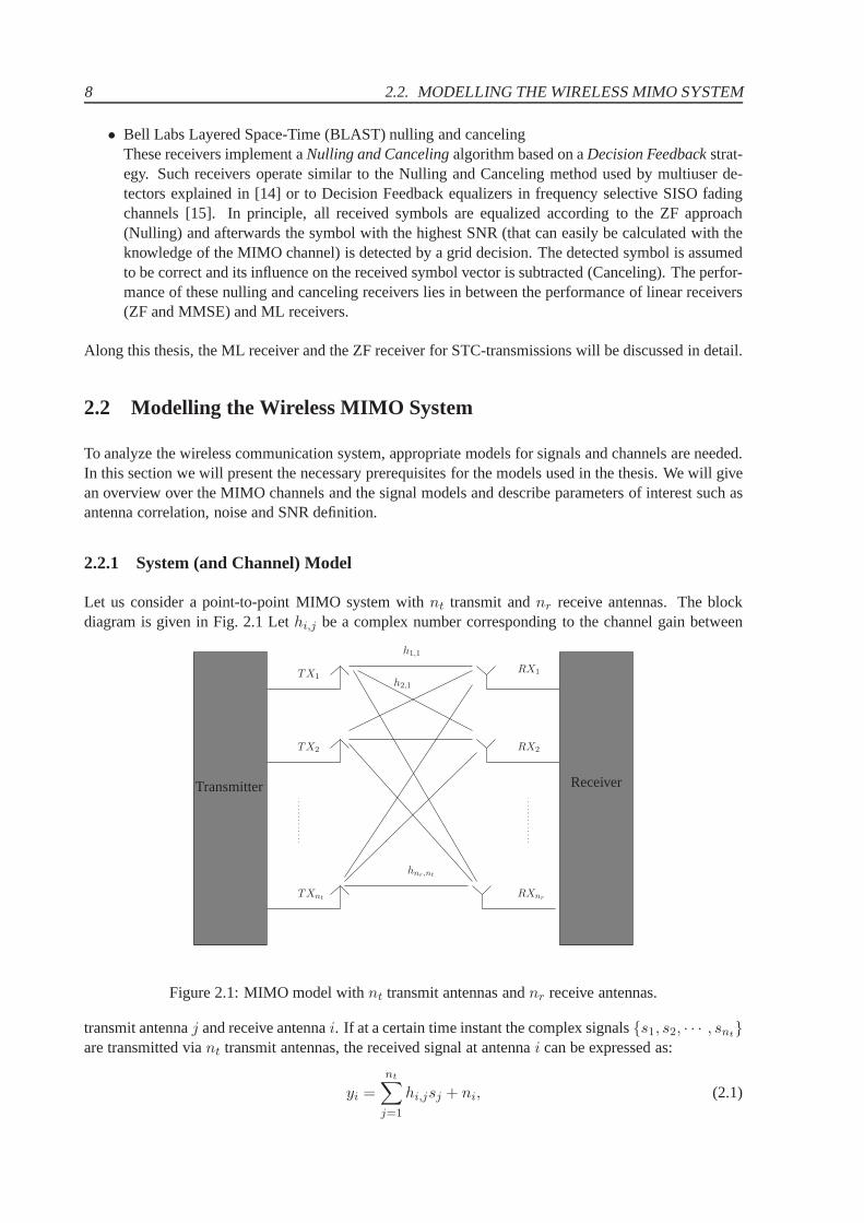
Let us consider a point-to-point MIMO system withnt transmit andnr receive antennas. The blockdiagram is given in Fig. 2.1 Lethi,j be a complex number corresponding to the channel gain between
Transmitter Receiver
TX1
TX2
TXnt
RX1
RX2
RXnr
h1,1
h2,1
hnr,nt
Figure 2.1: MIMO model withnt transmit antennas andnr receive antennas.
transmit antennaj and receive antennai. If at a certain time instant the complex signals{s1, s2, · · · , snt}are transmitted viant transmit antennas, the received signal at antennai can be expressed as:
yi =
nt∑
j=1
hi,jsj + ni, (2.1)
CHAPTER 2. MULTIPLE-ANTENNA WIRELESS COMMUNICATION SYSTEMS 9
whereni is a noise term (to be discussed later). Combining all receive signals in a vectory, (2.1) can beeasily expressed in matrix form
y = Hs + n. (2.2)
y is thenr × 1 receive symbol vector,H is thenr × nt MIMO channel transfer matrix,
H =
h1,1 · · · h1,nt
... · · · ...hnr ,1 · · · hnr ,nt
. (2.3)
s is thent × 1 transmit symbol vector andn is thenr × 1 additive noise vector. Note that the systemmodel implicitly assumes a flat fading MIMO channel, i.e., channel coefficients are constant during thetransmission of several symbols. Flat fading, or frequencynon-selective fading, applies by definition tosystems where the bandwidth of the transmitted signal is much smaller than the coherence bandwidth ofthe channel. All the frequency components of the transmitted signal undergo the same attenuation andphase shift propagation through the channel.Throughout this thesis, we assume that the transmit symbolsare uncorrelated, that means
E{ssH} = PsI, (2.4)
wherePs denotes the mean signal power of the used modulation format at each transmit antenna. Thisimplies that only modulation formats with the same mean power on all transmit antennas are considered.
2.2.2 Channel Model
In this thesis, two different spatial channel models are considered, namely spatially uncorrelated andspatially correlated channels.
2.2.2.1 Spatially Uncorrelated Channel
Spatially uncorrelated channels are modeled by a random matrix with independent identically distributed(i.i.d.), circularly symmetric, complex Gaussian entrieswith zero mean and unit variance [3], [2]:
H ∼ Nnr×ntC (0, 1). (2.5)
This is usually a rough approximation and such a model can be observed in scenarios where the antennaelements are located far apart from each other and a lot of scattering surround the antenna arrays atboth sides of the link. In practice, the elements ofH are correlated by an amount that depends on thepropagation environment as well as on the polarization of the antenna elements and the spacing betweenthem. For this reason it is necessary to consider correlatedchannels too.
2.2.2.2 Spatially Correlated Channel
In many implementations, the transmit and/or receive antennas can be spatially correlated. For exam-ple, in cellular systems, the base-station antennas are typically unhindered and have no local scatteringinducing correlation across the base-station antennas. Antenna correlation informs about the spatialdiversity available in a MIMO channel. If antennas are highly correlated, very small spatial diversitygain can be achieved. In principle, correlated MIMO channels can be modeled in two ways. There aregeometrically-based [17], [18] andstatistically-based [19], [20] channel models. In this thesis the focus
10 2.2. MODELLING THE WIRELESS MIMO SYSTEM
lies on statistical models.
Channel correlation models
A very simple and appropriate approach is to assume the entries of the channel matrix to be complexGaussian distributed with zero mean and unit variance with complex correlations between all entries[19]. The full correlation matrix can then be written as:
RH = E
h1hH1 h1h
H2 · · · h1h
Hnt
h2hH1 h2h
H2 · · · h2h
Hnt
......
.. ....
hnthH1 hnth
H2 · · · hnth
Hnt
(2.6)
wherehi denotes the i-th column vector of the channel matrix. Knowing all complex correlation coeffi-cients, the actual channel matrix can be modeled as:
H = (h1h2 · · ·hnt) with (hT1 hT
2 · · ·hTnt
)T = (RH)1/2g. (2.7)
g is an i.i.d. (nr · nt) × 1 random vector with complex Gaussian distributed entries with zero meanand unit variance. This model is called afull correlation model. The big drawback of this model is thata huge number of correlation parameters, namely(nr · nt)
2 parameters, are necessary to describe andgenerate the correlated channel matrices necessary for Monte Carlo simulations.
To reduce the huge number of necessary parameters, the so-called Kronecker Modelhas been intro-duced [19], [21], [22]. The assumption of this model is that the transmit and the receive correlation canbe separated. The model is described by the transmit correlation matrix
Rt = EH{HT H∗}, (2.8)
and the receive correlation matrix:Rr = EH{HHH}. (2.9)
Then, a correlated channel matrix can be generated as:
H =1
√
tr(Rr)R1/2
r V(R1/2t )T , (2.10)
where the matrixV is an i.i.d. random matrix with complex Gaussian entries with zero mean and unitvariance. With this approach the large number of model parameters is reduced ton2
r + n2t terms. A
big disadvantage of this correlation model is that MIMO channels with relatively high spatial correlationcannot be modeled adequately, due to the limiting heuristicassumption. More information about theKroncker model can be found in [23], [24].
In this thesis, we use the Kronecker model with the followingassumptions:The coefficients corresponding to adjacent transmit antennas are correlated according to:
Eh{|hi,j h∗i,j+1|} = ρt , j ∈ {1 . . . nt − 1}, (2.11)
ρt ∈ R , 0 ≤ ρt ≤ 1 .
independent from the receive antennai. In the same way the correlation of adjacent receive antennachannel coefficients is given by:
Eh{|hi,j h∗i+1,j|} = ρr , j ∈ {1 . . . nr − 1} (2.12)
CHAPTER 2. MULTIPLE-ANTENNA WIRELESS COMMUNICATION SYSTEMS 11
ρr ∈ R , 0 ≤ ρr ≤ 1 .
and does not depend on the transmit antenna indexj.In this way, we obtain specifically structured correlation matricesRt (transmit correlation matrix) andRr (receive correlation matrix):
Rt = RTt =
1 ρt ρ2t · · · ρnt−1
t
ρt 1 ρt · · · ρnt−2t
ρ2t ρt 1 · · · ρnt−3
t...
..... .
...ρnt−1
t ρnt−2t ρnt−3
t · · · 1
, (2.13)
Rr = RTr =
1 ρr ρ2r · · · ρnr−1
r
ρr 1 ρr · · · ρnr−2r
ρ2r ρr 1 · · · ρnr−3
r...
.... . .
...ρnr−1
r ρnr−2r ρnr−3
r · · · 1
, (2.14)
with real-valued correlation coefficients
ρt,ρr ∈ R , 0 ≤ ρt,ρr ≤ 1 .
TheseToeplitzstructured correlation matrices are quite appropriate formodelling the statistical behaviorwhen the antenna elements at the transmitter as well as at thereceiver are collocated linearly [25].
2.2.2.3 Noise Term and SNR-Definition
We assume the noise samples at the receive antennas to be spatially white circularly symmetric complexGaussian random variables with zero mean and varianceσ2
n:
n ∼ Nnr×1C (0, σ2
n). (2.15)
Such noise is calledadditive white Gaussian noise(AWGN). There are two strong reasons for this as-sumption. First, the Gaussian distribution tends to yield mathematical expressions that are easy to dealwith. Second, a Gaussian distribution of a disturbance termcan often be motivated via the central limittheorem of many statistical independent small contributions.
In this thesis, the simulation results are presented in terms of bit error ratios (BERs) either as afunction of the average SNR or as a function of the average SNRper bit, SNRbit. The average SNR isdefined as the ratio of the total received signal power and thetotal noise power:
SNR=EH,s
{
||y||22}
En
{
||n||22} =
EH,s
{
||Hs||22}
En
{
||n||22} , (2.16)
where||.||2 denotes thel2-norm operator. Assuming white Gaussian noise at each receive antenna anduncorrelated symbols with powerPs, (2.16) yields:
SNR=
∑nri=1
∑ntj=1 EH
{
|hi,j |22}
Ps
nrσ2n
. (2.17)
12 2.3. CHANNEL CAPACITY
Normalizing the MIMO channel matrix defined in (2.1) according toEH
{
|hi,j |22}
= 1, the final result
for the mean SNR is obtained as:
SNR=nrntPs
nrσ2n
=ntPs
σ2n
. (2.18)
Note that the SNR definition is symbol based and bit based definition is given by:
SNRbit =SNRld|A| (2.19)
where|A| denotes the cardinality of the modulation format.
2.3 Channel Capacity
Information-theoretic studies of wireless channels have been performed extensively. It has been shownthat the increase of MIMO capacity is huge compared to the capacity of a SISO system. One of themost important fields in the research area of MIMO systems is how to exploit this potential increase inchannel capacity in an efficient way. There are a lot of approaches, which can mainly be subdivided intospace-time coded and uncoded transmission systems.
The maximum error-free data rate that a channel can support is called thechannel capacity. Thechannel capacity for SISO AWGN channels was first derived by Claude Shannon [26]. In contrast toAWGN channels, multiple antenna channels combat fading andcover a spatial dimension.The capacity of a deterministic SISO channel with an input-output relationr = Hs + n is given by [2]
C = log2(1 + ρ|H|2) [bits/channel use] (2.20)
where the normalized channel power transfer characteristic is |H|2. The average SNR at each receiverbranch independent ofnt is ρ = P/σ2
n andP is the average power at the output of each receive antennas.The channel capacity of a deterministic MIMO channel is given by [2]:
C = log2
[
det(
Inr +ρ
ntHHH
)
]
[bits/channel use], (2.21)
and for random MIMO channels, the mean channel capacity, also calledthe ergodic capacity, is givenby [1]:
C = EH
{
log2
[
det(
Inr +ρ
ntHHH
)
]}
[bits/channel use], (2.22)
whereEH denotes expectation with respect toH. The ergodic capacity grows with the numbern ofantennas (under the assumptionnt = nr = n), which results in a significant capacity gain of MIMOfading channels compared to a wireless SISO transmission.The capacity of STBC will be discussed in detail in Chapter 6.
Example 2.1 Channel Cpacity of Spatially Uncorrelated MIMO Systems
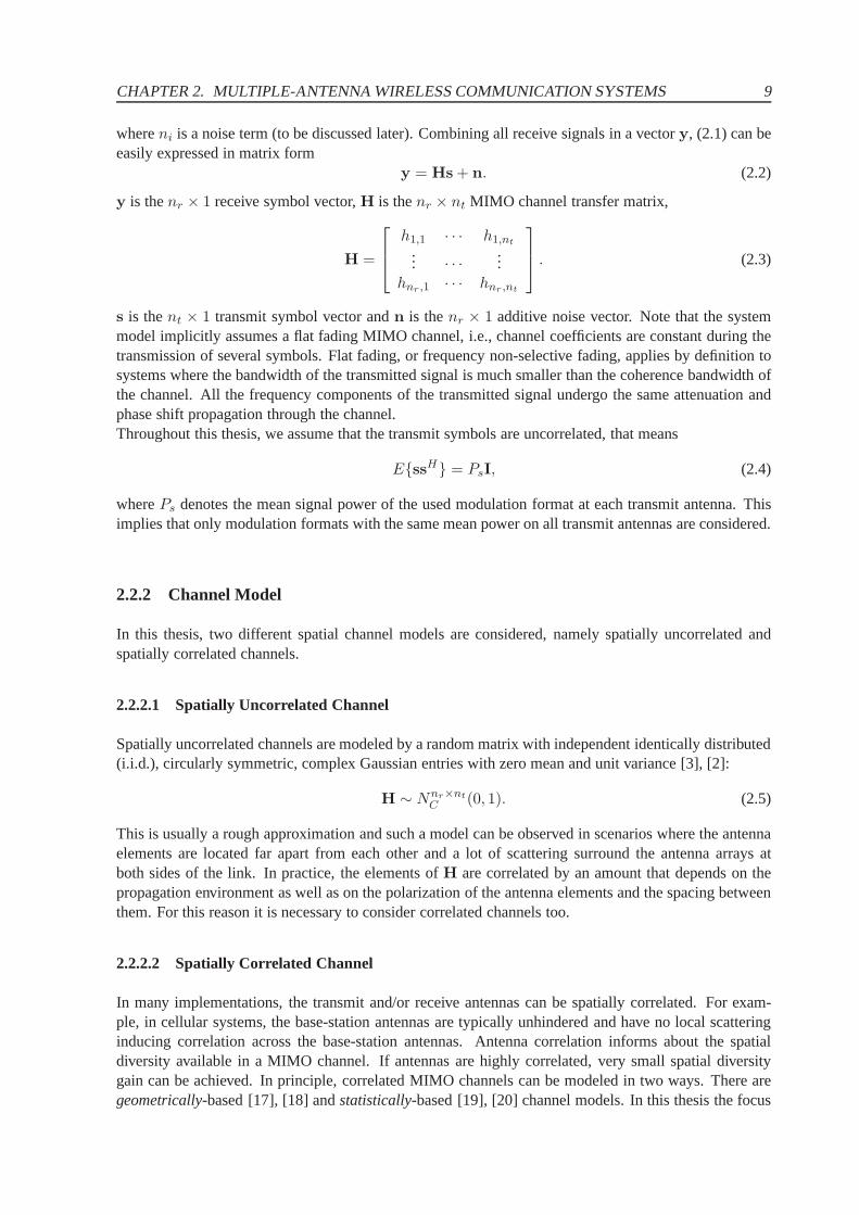
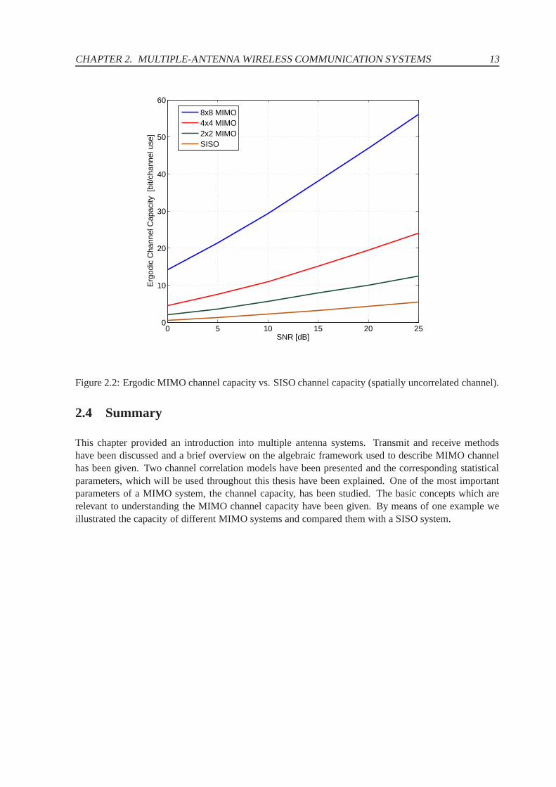
In Fig. 2.2 the ergodic channel capacity vs. the mean SNR is plotted for several uncorrelated MIMOsystems withnt = nr = n. The channel capacity for the SISO system (nt = nr = 1) at SNR=10 dBis approximately 2,95 bit /channel use. By applying multiple antennas, it is obvious that the channelcapacity increases substantially. A(4× 4) MIMO system (with four transmit and four receive antennas)can transmit more than 10,9 bit / channel use and the MIMO system with eight transmit and eight receiveantennas (8×8 MIMO) promises almost the ten fold capacity (29,7 bit / channel use) of the SISO channelat this SNR value.
CHAPTER 2. MULTIPLE-ANTENNA WIRELESS COMMUNICATION SYSTEMS 13
0 5 10 15 20 250
10
20
30
40
50
60
Erg
odic
Cha
nnel
Cap
acity
[bi
t/cha
nnel
use
]
SNR [dB]
8x8 MIMO4x4 MIMO2x2 MIMOSISO
Figure 2.2: Ergodic MIMO channel capacity vs. SISO channel capacity (spatially uncorrelated channel).
2.4 Summary
This chapter provided an introduction into multiple antenna systems. Transmit and receive methodshave been discussed and a brief overview on the algebraic framework used to describe MIMO channelhas been given. Two channel correlation models have been presented and the corresponding statisticalparameters, which will be used throughout this thesis have been explained. One of the most importantparameters of a MIMO system, the channel capacity, has been studied. The basic concepts which arerelevant to understanding the MIMO channel capacity have been given. By means of one example weillustrated the capacity of different MIMO systems and compared them with a SISO system.

14 2.4. SUMMARY
Chapter 3
Space-Time Coding
3.1 Introduction
Space-Time Codes (STCs) have been implemented in cellular communications as well as in wirelesslocal area networks. Space time coding is performed in both spatial and temporal domain introducingredundancy between signals transmitted from various antennas at various time periods. It can achievetransmit diversity and antenna gain over spatially uncodedsystems without sacrificing bandwidth. Theresearch on STC focuses on improving the system performanceby employing extra transmit antennas.In general, the design of STC amounts to finding transmit matrices that satisfy certain optimality criteria.Constructing STC, researcher have to trade-off between three goals: simple decoding, minimizing theerror probabilty, and maximizing the information rate. Theessential question is:How can we maximizethe transmitted date rate using a simple coding and decodingalgorithm at the same time as the bit errorprobability is minimized?
3.2 Space-Time Coded Systems
Let us consider a space-time coded communication system with nt transmit antennas andnr receiveantennas. The transmitted data are encoded by a space-time encoder. At each time slot, a block ofm ·nt
binary information symbolsct = [c1
t , c2t , · · · , cm·nt
t ]T (3.1)
is fed into the space-time encoder. The encoder maps the block of m binary data intont modulationsymbols from a signal set of constellationM = 2m points. After serial-to-parallel (SP) conversion, thent symbols
st = [s1t , s
2t , · · · , snt
t ]T 1 6 t 6 N (3.2)
are transmitted simultaneously during the slott from nt transmit antennas. Symbolsit, 1 6 i 6 nt,
is transmitted from antennai and all transmitted symbols have the same duration of T sec. The vectorin (3.2) is called aspace-time symboland by arranging the transmitted sequence in an array, ant × Nspace-time codeword matrix
S = [s1, s2, · · · , sN ] =
s11 s1
2 . . . s1N
s21 s2
2 . . . s2N
......
. . . . . .snt1 snt
2 . . . sntN
(3.3)
15
16 3.2. SPACE-TIME CODED SYSTEMS
can be defined. Thei-th rowsi = [si1, s
i2, · · · , si
N ] is the data sequence transmitted form thei-th transmitantenna and thej-th columnsj = [s1
j , s2j , · · · , snt
j ]T is the space-time symbol transmitted at timej, 1 6
j 6 N .As already explained in Section 2.2, the received signal vector can be calculated as
Y = HS + N. (3.4)
The MIMO channel matrixH corresponding tont transmit antennas andnr receive antennas can berepresented by annr × nt matrix:
H =
ht1,1 ht
1,2 . . . ht1,nt
ht2,1 ht
2,2 . . . ht2,nt
......
. . . . . .ht
nr ,1 htnr ,2 . . . ht
nr ,nt
, (3.5)
where theji-th element, denoted byhtj,i, is the fading gain coefficient for the path from transmit antenna
i to receive antennaj. We assume perfect channel knowledge at the receiver side and the transmitter hasno information about the channel available at the transmitter side. At the reciver, the decision metric iscomputed based on the squared Euclidian distance between all hypothesized receive sequences and theactual received sequence:
d2H =
∑
t
nr∑
j=1
∣
∣
∣yj
t −nt∑
i=1
htj,is
it
∣
∣
∣
2. (3.6)
Given the receive matrixY the ML-detector decides for the transmit matrixS with smallest Euclidiandistanced2
H .
3.2.1 Performance Analysis
To unterstand the properties of the STC, we will give an overview on the performance analysis first de-veloped by Tarokh [3] and Vucetic [27].
For the performance analysis of STCs it is important to evaluate thepairwise error probability(PEP). The pairwise error probabilityP (S, S) is the probability that the decoder selects a codewordS = [s1, s2, · · · , sN ], when the transmitted codeword was in factS = [s1, s2, · · · , sN ] 6= S.Assuming that the matrixH = [h1,h2, . . . ,hN ] is known, than the conditional pairwise error probabilityis given as:
P (S, S|H) = Q
(
√
Es
2N0d2
H(S, S)
)
, (3.7)
whered2H(S, S) is given by
d2H(S, S) = ||H(S − S)||2F (3.8)
=
N∑
t=1
nr∑
j=1
∣
∣
∣
∣
∣
nt∑
i=1
hti,j(s
it − si
t)
∣
∣
∣
∣
∣
2
, (3.9)
whereEs is the energy per symbol at each transmit antenna,N0 is noise power spectral density andQ(x)is the complementary error function defined by:
Q(x) =1√2π
∫ ∞
xe−t2/2dt. (3.10)
CHAPTER 3. SPACE-TIME CODING 17
By applying the bound
Q(x) 61
2e−x2/2, x > 0, (3.11)
the PEP in (3.7) becomes
P (S, S|H) 61
2exp
(
− d2H(S, S)
Es
4N0
)
. (3.12)
3.2.1.1 Error Probability for Slow Fading Channels
If slow fading is assumed, the fading coefficients are assumed to be constant duringNs symbols andvary from one symbol block to another, which means that the symbol period is small compared to thechannel coherence time. Since the fading coefficients within each frame are constant the superscriptt ofthe fading coefficients can be ignored:
h1j,i = h2
j,i = · · · = hNj,i = hj,i, i = 1, 2, · · · , nt, j = 1, 2, · · · , nr. (3.13)
Let us define ant × N codeword difference matrixB:
B(S, S) = S− S =
s11 − s1
1 s12 − s1
2 · · · s1N − s1
N
s21 − s2
1 s22 − s2
2 · · · s2N − s2
N...
.... . .
...snt1 − snt
1 snt2 − snt
2 · · · sntN − snt
N
. (3.14)
Next, ant × nt code distance matrixA is defined as:
A = BBH , (3.15)
where the superscript H denotes the Hermitian (transpose conjugate) of a matrix.A is a nonnegativedefinite Hermitian matrix, sinceA = AH and the eigenvalues ofA are nonnegative real numbers [28] .Therefore, there exits a unitary matrixU and a real diagonal matrix∆ such that
UAUH = ∆. (3.16)
The rows ofU, {u1,u2, · · · ,unt} are the eigenvectors ofA. The diagonal elements of∆, denoted asλi, i = 1, 2, · · · , nt are the eigenvalues ofA. Let r denote the rank of the matrixA. Then there existrreal, nonnegative eigenvaluesλ1, λ2, · · · , λr.With hj = [hj,1, hj,2, · · · .hj,nt]
T andβj,i = hj · ui Eqn. (3.9)1 can be rewritten as
d2H(S, S) =
nr∑
j=1
r∑
i=1
λi|βj,i|2. (3.17)
Substituting (3.17) in (3.12) we obtain
P (S, S) 61
2exp
(
−nr∑
j=1
r∑
i=1
λi|βj,i|2Es
4N0
)
. (3.18)
Inequality (3.18) is an upper bound on the conditional pairwise error probability expressed as a func-tion of |βj,i|. Assuming knowledge ofhj,i we can determine the distribution of|βj,i|. Note that, forU = const, and assuming thathj,i are complex Gaussian random variables with meanµj,i
h and variance1/2 per dimension and{u1,u2, · · · ,unt} is an orthonormal basis of an N-dimensional vector space.
1· denotes the inner product of complex-valued vectors
18 3.2. SPACE-TIME CODED SYSTEMS
Therefore|βj,i| are independent complex Gaussian random variables with variance1/2 per dimensionand meanµj,i
β ,
µj,iβ = E[hj ] · E[ui] = [µj,1
h , µj,2h , · · · , µj,nt
h ] · ui (3.19)
whereE[·] denotes the expectation. LetKj,i = |µj,ih |2, then |βj,i| has a Rician distribution with the
probability density function(pdf) [30]
p(|βj,i|) = 2|βj,i|exp(−|βj,i|2 − Ki,j)I0(2|βj,i|√
Ki,j). (3.20)
To compute an upper bound on the mean probability of error, wehave simply to average over
nr∏
j=1
exp
((
Es
4N0
)
nt∑
i=1
λi|βj,i|2)
. (3.21)
For the special case of flat Rayleigh fading withE[hi,j ] = 0 andKi,j = 0 for all i andj, the PEP canbe bounded by [3]
P (s, s) 6
(
r∏
i=1
λi
)−nr(
Es
4N0
)−rnr
(3.22)
wherer denotes the rank of the matrixA(S,S) andλ1, λ2, · · · , λr are the nonzero eigenvalues of thematrixA(S,S).
From (3.22) two most important parameters of a STC can be defined:
• The diversity gainis equal tornr. It determines the slope of the mean PEP over SNR curve. It isan approximate measure of a power gain of the system with space diversity compared to systemwithout diversity measured at the same error probability value.
• The coding gainis (∏r
i=1 λi)1/r. It determines a horizontal shift of the mean PEP curve for a
coded system relative to an uncoded system with the same diversity gain.
To minimize the PEP, it is preferable to make both diversity gain and coding gain as large as possible.Since the diversity gain is an exponent in the error probability upper bound (3.22), it is obvious that inthe high SNR range achieving a large diversity gain is more important than achieving a high coding gain.
3.2.1.2 Error Probability for Fast Fading Channels
In a fast fading channel, the fading coefficients are constant within each symbol period but vary from onesymbol to another. At each timet thespace-time symbol difference vectorf(st, st) is
f(st, st) =[
s1t − s1
t , s2t − s2
t , · · · , sntt − snt
t
]
. (3.23)
Let us consider annt × nt matrixC(st,st) defined as:
C(st,st) = f(st, st)fH(st, st). (3.24)
It is clear that the matrixC(st,st) is Hermitian and there exists a unitary matrixUt and a real-valueddiagonal matrixDt, such that:
UtC(st,st)UHt = Dt. (3.25)
CHAPTER 3. SPACE-TIME CODING 19
The diagonal elements ofDt are the eigenvaluesDit, i = 1, 2, · · · , nt, and the rows ofUt, {u1
t ,u2
t , · · · ,untt }, are the eigenvectors ofC(st, st), which form a complete orthonormal basis of an
nt -dimensional vector space.In the casest = st, C(st,st) is an all-zero matrix and all the eigenvaluesDi
t are zero. On the other hand,if st 6= st the matrixC(st,st) has only one nonzero eigenvalue and the othernt − 1 eigenvalues arezero. LetD1
t be the single nonzero eigenvalue element which is equal to the squared Euclidian distancebetween the two space-time symbolsst andst:
D1t = ||st − st||2 =
nt∑
i=1
||sit − si
t||2. (3.26)
The eigenvector ofC(st, st) corresponding to the nonzero eigenvalueD1t is denoted byu1
t , hjt is defined
ashjt = [ht
j,1, htj,2, · · · , ht
j,nt] andβt
j,i = hjt · ui
t. Sincehi,j are samples of a complex Gaussian randomvariable with meanE[hi,j ] and sinceUt is unitary, it follows thatβt
j,i are independent Gaussian randomvariables with variance1/2 per dimension. The mean ofβt
j,i can be easily computed from the mean of
hjt and the matrixC(st,st) [27].
Assuming fast fading, the modified Euclidian distance in (3.9) can be rewritten as:
d2H(S,S) =
N∑
t=1
nr∑
j=1
nt∑
i
|βtj,i|2 · Di
t. (3.27)
Since at each timet there is at most only one nonzero eigenvalueD1t , the (3.27) can be represented as:
d2H(S,S) =
N∑
t∈ρ(s,s)
nr∑
j=1
|βtj,i|2 · D1
t
=
N∑
t∈ρ(s,s)
nr∑
j=1
|βtj,i|2 · ||st − st||2 (3.28)
whereρ(s, s) denotes the set of time instancest = 1, 2, · · · , N where||st − st|| 6= 0. Substituting (3.28)into (3.7), we obtain:
P (S, S|H) 61
2exp
(
−∑
t∈ρ(s,s)
nr∑
j=1
λi|βj,i|2||st − st||2Es
4N0
)
. (3.29)
DenotingδH as the number of the space-time symbols in wich two code wordsS andS differ, then atthe right side of inequality (3.29), there areδHnr different random variables. The termδH is calledspace-time symbol-wise Hamming distancebetween two code words [27].
For a special case where|βtj,i| are Rayleigh distributed, the upper bound of the pairwise error proba-
bility at high SNR’s becomes [3]
P (S, S) 6∏
t∈ρ(s,s)
|st − st|−2nr
(
Es
4N0
)−δHnr
= d−2nrp
(
Es
4N0
)−δHnr
, (3.30)
20 3.3. SPACE-TIME BLOCK CODES
whered2p is the product of the squared Euclidian distances between the two space-time symbol sequences
and it is given by
d2p =
∏
t∈ρ(s,s)
|st − st|2. (3.31)
The termδHnr is called thediversity gainin case of fast fading channels and
Gc =d21/δH
p
d2u
(3.32)
is calledcoding gain, whered2u is the squared Euclidian distance of the uncoded reference system.
Diversity and coding gains are obtained as the minimum ofδHnr andd21/δHp over all pairs of distinct
codewords [3], [27].
The optimal code design in fading channels depends on the possible diversity gain (total diversity)of the STC system. For codes on slow fading channels, the total diversity is the product of the receivediversity,nr, and the transmit diversityr provided by the coding scheme (3.22). For codes on fast fadingchannels, the total diversity is the product of the receive diversitynr, and the time diversityδH , achievedby the coding scheme (3.30). For small values of total diversity and slow fading channels, the diversityand the coding gain should be maximized by choosing a code with the largest minimum rank and thelargest determinant of the distance matrixA. For fast fading channels, a code with the largest minimumsymbol-wise Hamming distance and the largest product distance should be chosen. Further details aboutcode design can be found in [3] and in [27].
3.2.2 Space-Time Codes
Essentially, two different space-time coding methods, namely space-time trellis codes (STTCs) andspace-time block codes (STBCs) have been proposed. STTC hasbeen introduced in [3] as a codingtechnique that promises full diversity and substantial coding gain at the price of a quite high decodingcomplexity. To avoid this disadvantage, STBCs have been proposed by the pioneering work of Alamouti[29]. The Alamouti code promises full diversity and full data rate (on data symbol per channel use) incase of two transmit antennas. The key feature of this schemeis the orthogonality between the signalvectors transmitted over the two transmit antennas. This scheme was generalized to an arbitrary numberof transmit antennas by applying the theorie oforthogonal design[40]. The generalized schemes arereferred to asspace-time block codes[32]. However, for more than two transmit antennas no complex-valued STBCs with full diversity and full data rate exist. Thus, many different code design methodshave been proposed providing either full diversity or full data rate [31], [32], [33], [34]. In our opinion,the essential of STBCs is the provision of full diversity with extremely low encoder/decoder complex-ity, what will be discussed in this thesis afterwards. If we want to increase the coding gain further, weshould apply an additional high performance outer code concatenated with an appropriate STBC used asan inner code. Such schemes have been proposed e.g. under thename of Super Orthogonal Space-TimeTrellis Codes [35].
3.3 Space-Time Block Codes
In a general form, an STBC can be seen as a mapping ofnN complex symbols{s1, s2, · · · , sN} onto amatrixS of dimensionnt × N :
{s1, s2, · · · , sN} → S (3.33)
CHAPTER 3. SPACE-TIME CODING 21
An STBC code matrixS taking on the following form:
S =
nN∑
n=1
(snAn + jsnBn), (3.34)
where{s1, s2, · · · , snN} is a set of symbols to be transmitted withsn = Re{sn} and sn = Im{sn} ,
and with fixed code matrices{An,Bn} of dimensionnt × N are called linear STBCs. The followingSTBCs can be regarded as special cases of these codes.
3.3.1 Alamouti Code
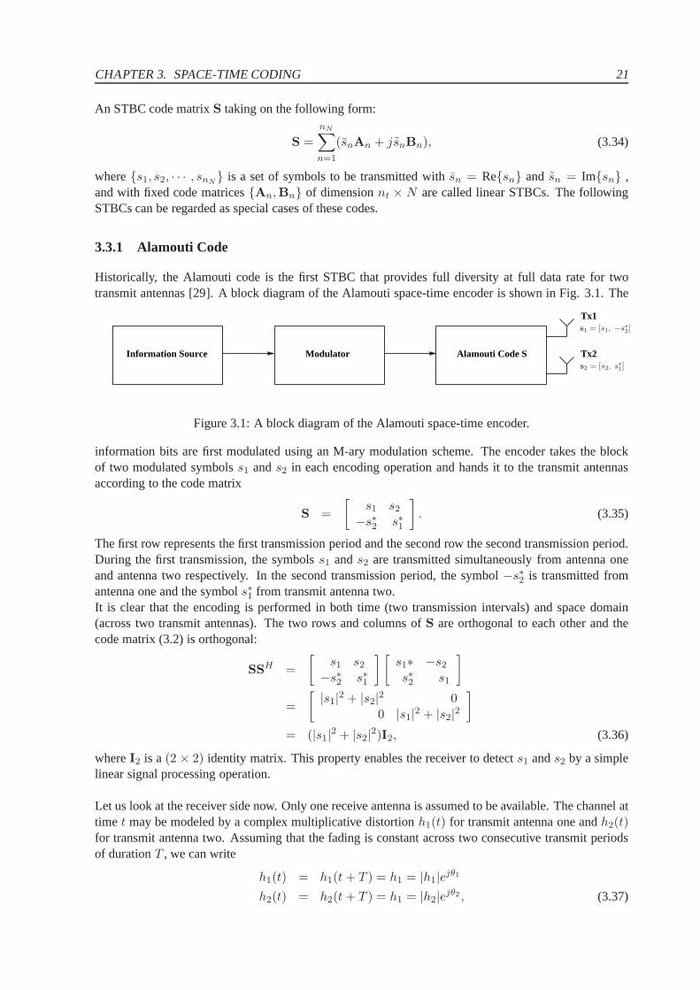
Historically, the Alamouti code is the first STBC that provides full diversity at full data rate for twotransmit antennas [29]. A block diagram of the Alamouti space-time encoder is shown in Fig. 3.1. The
Alamouti Code SModulatorInformation Source Tx2
Tx1s1 = [s1, −s∗2]
s2 = [s2, s∗1]
Figure 3.1: A block diagram of the Alamouti space-time encoder.
information bits are first modulated using an M-ary modulation scheme. The encoder takes the blockof two modulated symbolss1 ands2 in each encoding operation and hands it to the transmit antennasaccording to the code matrix
S =
[
s1 s2
−s∗2 s∗1
]
. (3.35)
The first row represents the first transmission period and thesecond row the second transmission period.During the first transmission, the symbolss1 ands2 are transmitted simultaneously from antenna oneand antenna two respectively. In the second transmission period, the symbol−s∗2 is transmitted fromantenna one and the symbols∗1 from transmit antenna two.It is clear that the encoding is performed in both time (two transmission intervals) and space domain(across two transmit antennas). The two rows and columns ofS are orthogonal to each other and thecode matrix (3.2) is orthogonal:
SSH =
[
s1 s2
−s∗2 s∗1
] [
s1∗ −s2
s∗2 s1
]
=
[
|s1|2 + |s2|2 00 |s1|2 + |s2|2
]
= (|s1|2 + |s2|2)I2, (3.36)
whereI2 is a(2 × 2) identity matrix. This property enables the receiver to detect s1 ands2 by a simplelinear signal processing operation.
Let us look at the receiver side now. Only one receive antennais assumed to be available. The channel attime t may be modeled by a complex multiplicative distortionh1(t) for transmit antenna one andh2(t)for transmit antenna two. Assuming that the fading is constant across two consecutive transmit periodsof durationT , we can write
h1(t) = h1(t + T ) = h1 = |h1|ejθ1
h2(t) = h2(t + T ) = h1 = |h2|ejθ2 , (3.37)
22 3.3. SPACE-TIME BLOCK CODES
where|hi| andθi, i = 1, 2 are the amplitude gain and phase shift for the path from transmit antennai tothe receive antenna. The received signals at the timet andt + T can then be expressed as
r1 = s1h1 + s2h2 + n1
r2 = −s∗2h1 + s∗1h2 + n2, (3.38)
wherer1 andr2 are the received signals at timet andt + T , n1 andn2 are complex random variablesrepresenting receiver noise and interference. This can be written in matrix form as:
r = Sh + n, (3.39)
whereh = [h1,h2]T is the complex channel vector andn is the noise vector at the receiver.
3.3.2 Equivalent Virtual (2 × 2) Channel Matrix (EVCM) of the Alamouti Code
Conjugating the signalr2 in (3.38) that is received in the second symbol period, the received signal maybe written equivalently as
r1 = h1s1 + h2s2 + n1
r∗2 = −h∗1s2 + h∗
2s1 + n2. (3.40)
Thus the equation (3.40) can be written as
[
r1
r∗2
]
=
[
h1 h2
h∗2 −h∗
1
] [
s1
s2
]
+
[
n1
n2
]
or in short notation:
y = Hvs + n, (3.41)
where the modified receive vectory = [r1, r∗2]
T has been introduced.Hv will be termed the equivalentvirtual MIMO channel matrix (EVCM) of the Alamouti STBC scheme. It is given by:
Hv =
[
h1 h2
h∗2 −h∗
1
]
. (3.42)
Thus, by considering of the elements ofy in (3.41) as originating from two virtual receive antennas(instead of received samples at one antenna at two time slots) one could interpret the(2 × 1) AlamoutiSTBC as a(2× 2) spatial multiplexing transmission using one time slot. Thekey difference between theAlamouti scheme and a true(2× 2) multiplexing system lies in the specific structure ofHv. Unlike to ageneral i.i.d. MIMO channel matrix, the rows and columns of the virtual channel matrix are orthogonal:
HvHHv = HH
v Hv = (|h1|2 + |h2|2)I2 = |h|2I2 , (3.43)
whereI2 is the(2 × 2) identity matrix andh2 is the power gain of the equivalent MIMO channel withh2 = |h1|2 + |h2|2. Due to this orthogonality the receiver of the Alamouti scheme (discussed in detailin the following subsection) decouples the MISO channel into two virtually independent channels eachwith channel gainh2 and diversityd = 2.It is obvious that the EVCM depends on the structure of the code and the channel coefficients. Theconcept of the EVCM simplifies the analysis of the STBC transmission scheme. The existence of anEVCM is one of the important characteristics of STBCs and will be frequently used in this thesis.
CHAPTER 3. SPACE-TIME CODING 23
3.3.3 Linear Signal Combining and Maximum Likelihood Decoding of the AlamoutiCode
If the channel coefficientsh1 and h2 can be perfectly estimated at the receiver, the decoder can usethem as channel state information (CSI). Assuming that all the signals in the modulation constellationare equiprobable, a maximum likelihood (ML) detector decides for that pair of signals(s1, s2) from thesignal modulation constellation that minimizes the decision metric
d2(r1, h1s1 + h2s2) + d2(r2,−h1s∗2 + h2s
∗1) = |r1 − h1s1 − h2s2|2 + |r2 + h1s
∗2 − h2s
∗1|2, (3.44)
whered(x1, x2) = |x1 − x2|. On the other hand, using a linear receiver, the signal combiner at thereceiver combines the received signalsr1 andr2 as follows
s1 = h∗1r1 + h2r
∗2 = (|h1|2 + |h2|2)s1 + h∗
1n1 + h2n∗2
s2 = h∗2r1 − h1r
∗2 = (|h1|2 + |h2|2)s2 − h1n
∗2 + h∗
2n1. (3.45)
Hences1 ands2 are two decisions statistics constructed by combining the received signals with coeffi-cients derived from the channel state information. These noisy signals are sent to ML detectors and thusthe ML decoding rule (3.45) can be separated into two independent decoding rules fors1 ands2, namely
s1 = argmins1∈S
d2(s1, s1) (3.46)
for detectings1, and
s2 = argmins2∈S
d2(s2, s2) (3.47)
for detectings2.
The Alamouti transmission scheme is a simple transmit diversity scheme which improves the signalquality at the receiver using a simple signal processing algorithm (STC) at the transmitter. The diversityorder obtained is equal to that one applying maximal ratio combining (MRC) with one antenna at thetransmitter and two antennas at the receiver where the resulting signals at the receiver are:
r1 = h1s1 + n1 (3.48)
r2 = h2s1 + n2 (3.49)
and the combined signal is
s1 = h∗1r1 + h∗
2r2
= (|h1|2 + |h2|2)s1 + h∗1n1 + h∗
2n2. (3.50)
The resulting combined signals in (3.45) are equivalent to those obtained from a two-branch MRC in(3.50). The only difference are phase rotations on the noisecomponents which do not degrade the ef-fective SNR. Therefore, the resulting diversity order obtained by the Alamouti scheme with one receiveris equal to that of a two-branch MRC at the receiver. We confirmthis statement by simulating the BERperformance of the Alamouti scheme.
Example 3.1 BER Performance of the Alamouti Scheme
The performance of the Alamouti scheme using QPSK symbols, Gray coding and averaged over 10.000channel realizations obtained by simulations of slow Rayleigh fading channels is shown in Fig. 3.2. It
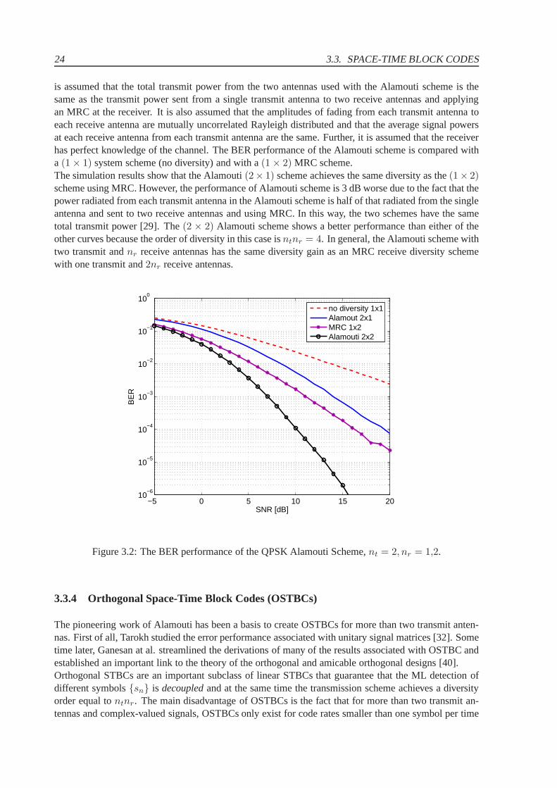
24 3.3. SPACE-TIME BLOCK CODES
is assumed that the total transmit power from the two antennas used with the Alamouti scheme is thesame as the transmit power sent from a single transmit antenna to two receive antennas and applyingan MRC at the receiver. It is also assumed that the amplitudesof fading from each transmit antenna toeach receive antenna are mutually uncorrelated Rayleigh distributed and that the average signal powersat each receive antenna from each transmit antenna are the same. Further, it is assumed that the receiverhas perfect knowledge of the channel. The BER performance ofthe Alamouti scheme is compared witha (1 × 1) system scheme (no diversity) and with a(1 × 2) MRC scheme.The simulation results show that the Alamouti(2× 1) scheme achieves the same diversity as the(1× 2)scheme using MRC. However, the performance of Alamouti scheme is 3 dB worse due to the fact that thepower radiated from each transmit antenna in the Alamouti scheme is half of that radiated from the singleantenna and sent to two receive antennas and using MRC. In this way, the two schemes have the sametotal transmit power [29]. The(2 × 2) Alamouti scheme shows a better performance than either of theother curves because the order of diversity in this case isntnr = 4. In general, the Alamouti scheme withtwo transmit andnr receive antennas has the same diversity gain as an MRC receive diversity schemewith one transmit and2nr receive antennas.
−5 0 5 10 15 2010
−6
10−5
10−4
10−3
10−2
10−1
100
SNR [dB]
BE
R
no diversity 1x1Alamout 2x1MRC 1x2Alamouti 2x2
Figure 3.2: The BER performance of the QPSK Alamouti Scheme,nt = 2, nr = 1,2.
3.3.4 Orthogonal Space-Time Block Codes (OSTBCs)
The pioneering work of Alamouti has been a basis to create OSTBCs for more than two transmit anten-nas. First of all, Tarokh studied the error performance associated with unitary signal matrices [32]. Sometime later, Ganesan at al. streamlined the derivations of many of the results associated with OSTBC andestablished an important link to the theory of the orthogonal and amicable orthogonal designs [40].Orthogonal STBCs are an important subclass of linear STBCs that guarantee that the ML detection ofdifferent symbols{sn} is decoupledand at the same time the transmission scheme achieves a diversityorder equal tontnr. The main disadvantage of OSTBCs is the fact that for more than two transmit an-tennas and complex-valued signals, OSTBCs only exist for code rates smaller than one symbol per time
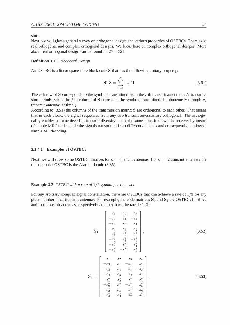
CHAPTER 3. SPACE-TIME CODING 25
slot.Next, we will give a general survey on orthogonal design and various properties of OSTBCs. There existreal orthogonal and complex orthogonal designs. We focus here on complex orthogonal designs. Moreabout real orthogonal design can be found in [27], [32].
Definition 3.1 Orthogonal Design
An OSTBC is a linear space-time block codeS that has the following unitary property:
SHS =N∑
n=1
|sn|2I (3.51)
Thei-th row ofS corresponds to the symbols transmitted from thei-th transmit antenna inN transmis-sion periods, while thej-th column ofS represents the symbols transmitted simultaneously through nt
transmit antennas at timej.According to (3.51) the columns of the transmission matrixS are orthogonal to each other. That meansthat in each block, the signal sequences from any two transmit antennas are orthogonal. The orthogo-nality enables us to achieve full transmit diversity and at the same time, it allows the receiver by meansof simple MRC to decouple the signals transmitted from different antennas and consequently, it allows asimple ML decoding.
3.3.4.1 Examples of OSTBCs
Next, we will show some OSTBC matrices fornt = 3 and4 antennas. Fornt = 2 transmit antennas themost popular OSTBC is the Alamouti code (3.35).
Example 3.2 OSTBC with a rate of1/2 symbol per time slot
For any arbitrary complex signal constellation, there are OSTBCs that can achieve a rate of1/2 for anygiven number ofnt transmit antennas. For example, the code matricesS3 andS4 are OSTBCs for threeand four transmit antennas, respectively and they have the rate1/2 [3].
S3 =
s1 s2 s3
−s2 s1 −s4
−s3 s4 s1
−s4 −s3 s2
s∗1 s∗2 s∗3−s∗2 s∗1 −s∗4−s∗3 s∗4 s∗1−s∗4 −s∗3 s∗2
, (3.52)
S4 =
s1 s2 s3 s4
−s2 s1 −s4 s3
−s3 s4 s1 −s2
−s4 −s3 s2 s1
s∗1 s∗2 s∗3 s∗4−s∗2 s∗1 −s∗4 s∗3−s∗3 s∗4 s∗1 −s∗2−s∗4 −s∗3 s∗2 s∗1
. (3.53)
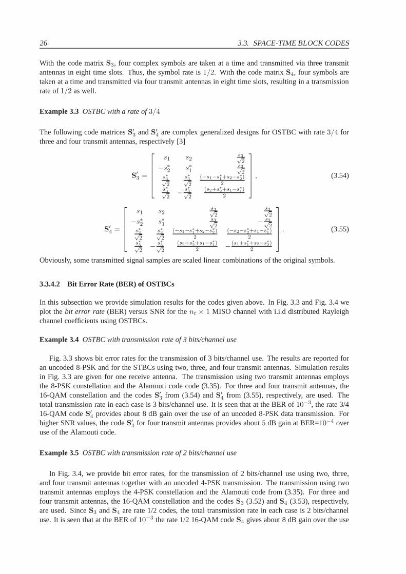
26 3.3. SPACE-TIME BLOCK CODES
With the code matrixS3, four complex symbols are taken at a time and transmitted viathree transmitantennas in eight time slots. Thus, the symbol rate is1/2. With the code matrixS4, four symbols aretaken at a time and transmitted via four transmit antennas ineight time slots, resulting in a transmissionrate of1/2 as well.
Example 3.3 OSTBC with a rate of3/4
The following code matricesS′3 andS′
4 are complex generalized designs for OSTBC with rate3/4 forthree and four transmit antennas, respectively [3]
S′3 =
s1 s2s3√2
−s∗2 s∗1s3√2
s∗3√2
s∗3√2
(−s1−s∗1+s2−s∗
2)
2s∗3√2
− s∗3√2
(s2+s∗2+s1−s∗
1)
2
, (3.54)
S′4 =
s1 s2s3√2
s3√2
−s∗2 s∗1s3√2
− s3√2
s∗3√2
s∗3√2
(−s1−s∗1+s2−s∗
2)
2(−s2−s∗
2+s1−s∗
1)
2s∗3√2
− s∗3√2
(s2+s∗2+s1−s∗
1)
2 − (s1+s∗1+s2−s∗
2)
2
. (3.55)
Obviously, some transmitted signal samples are scaled linear combinations of the original symbols.
3.3.4.2 Bit Error Rate (BER) of OSTBCs
In this subsection we provide simulation results for the codes given above. In Fig. 3.3 and Fig. 3.4 weplot thebit error rate (BER) versus SNR for thent × 1 MISO channel with i.i.d distributed Rayleighchannel coefficients using OSTBCs.
Example 3.4 OSTBC with transmission rate of 3 bits/channel use
Fig. 3.3 shows bit error rates for the transmission of 3 bits/channel use. The results are reported foran uncoded 8-PSK and for the STBCs using two, three, and four transmit antennas. Simulation resultsin Fig. 3.3 are given for one receive antenna. The transmission using two transmit antennas employsthe 8-PSK constellation and the Alamouti code code (3.35). For three and four transmit antennas, the16-QAM constellation and the codesS′
3 from (3.54) andS′4 from (3.55), respectively, are used. The
total transmission rate in each case is 3 bits/channel use. It is seen that at the BER of10−3, the rate 3/416-QAM codeS′
4 provides about 8 dB gain over the use of an uncoded 8-PSK data transmission. Forhigher SNR values, the codeS′
4 for four transmit antennas provides about5 dB gain at BER=10−4 overuse of the Alamouti code.
Example 3.5 OSTBC with transmission rate of 2 bits/channel use
In Fig. 3.4, we provide bit error rates, for the transmissionof 2 bits/channel use using two, three,and four transmit antennas together with an uncoded 4-PSK transmission. The transmission using twotransmit antennas employs the 4-PSK constellation and the Alamouti code from (3.35). For three andfour transmit antennas, the 16-QAM constellation and the codesS3 (3.52) andS4 (3.53), respectively,are used. SinceS3 andS4 are rate 1/2 codes, the total transmission rate in each case is 2 bits/channeluse. It is seen that at the BER of10−3 the rate 1/2 16-QAM codeS4 gives about 8 dB gain over the use
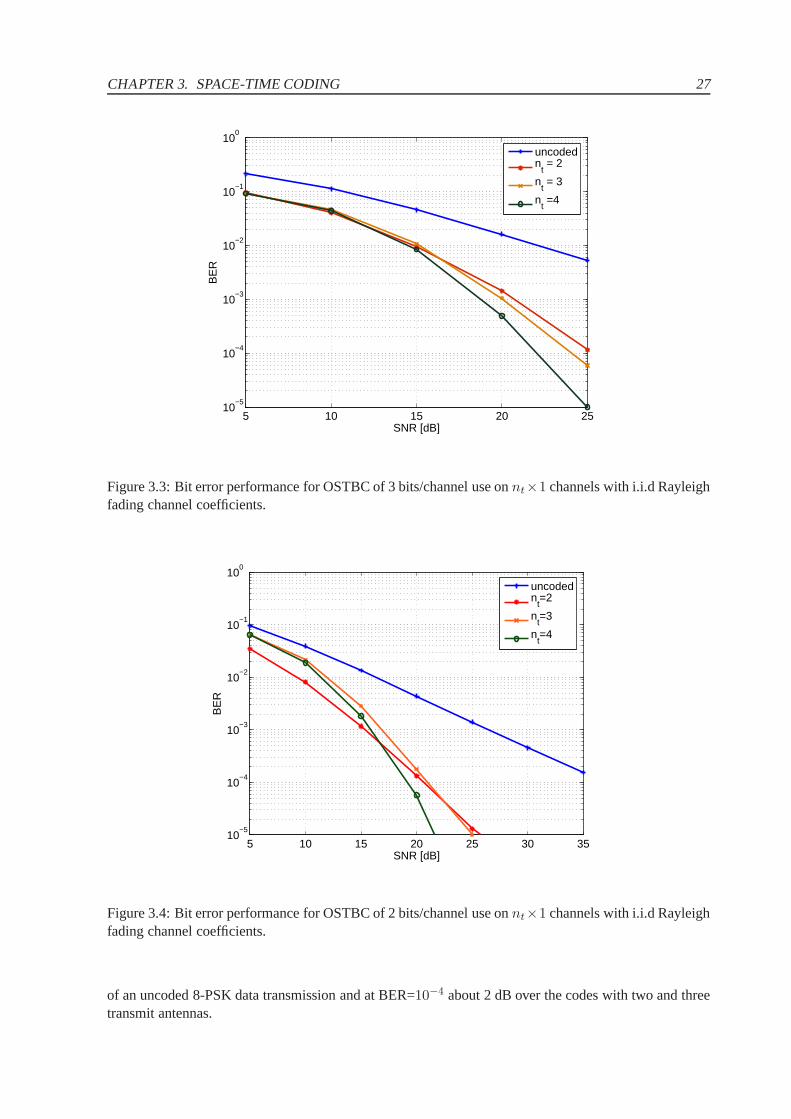
CHAPTER 3. SPACE-TIME CODING 27
5 10 15 20 2510
−5
10−4
10−3
10−2
10−1
100
SNR [dB]
BE
R
uncodedn
t = 2
nt = 3
nt =4
Figure 3.3: Bit error performance for OSTBC of 3 bits/channel use onnt×1 channels with i.i.d Rayleighfading channel coefficients.
5 10 15 20 25 30 3510
−5
10−4
10−3
10−2
10−1
100
SNR [dB]
BE
R
uncodedn
t=2
nt=3
nt=4
Figure 3.4: Bit error performance for OSTBC of 2 bits/channel use onnt×1 channels with i.i.d Rayleighfading channel coefficients.
of an uncoded 8-PSK data transmission and at BER=10−4 about 2 dB over the codes with two and threetransmit antennas.
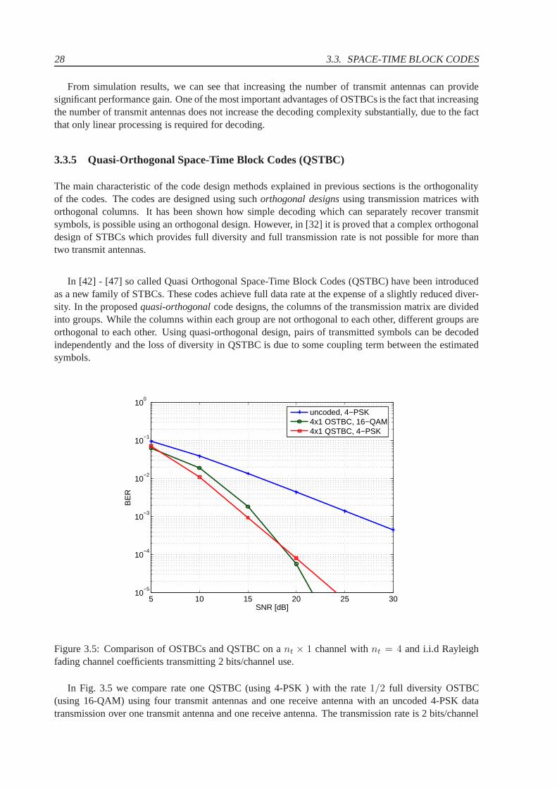
28 3.3. SPACE-TIME BLOCK CODES
From simulation results, we can see that increasing the number of transmit antennas can providesignificant performance gain. One of the most important advantages of OSTBCs is the fact that increasingthe number of transmit antennas does not increase the decoding complexity substantially, due to the factthat only linear processing is required for decoding.
3.3.5 Quasi-Orthogonal Space-Time Block Codes (QSTBC)
The main characteristic of the code design methods explained in previous sections is the orthogonalityof the codes. The codes are designed using suchorthogonal designsusing transmission matrices withorthogonal columns. It has been shown how simple decoding which can separately recover transmitsymbols, is possible using an orthogonal design. However, in [32] it is proved that a complex orthogonaldesign of STBCs which provides full diversity and full transmission rate is not possible for more thantwo transmit antennas.
In [42] - [47] so called Quasi Orthogonal Space-Time Block Codes (QSTBC) have been introducedas a new family of STBCs. These codes achieve full data rate atthe expense of a slightly reduced diver-sity. In the proposedquasi-orthogonalcode designs, the columns of the transmission matrix are dividedinto groups. While the columns within each group are not orthogonal to each other, different groups areorthogonal to each other. Using quasi-orthogonal design, pairs of transmitted symbols can be decodedindependently and the loss of diversity in QSTBC is due to some coupling term between the estimatedsymbols.
5 10 15 20 25 3010
−5
10−4
10−3
10−2
10−1
100
SNR [dB]
BE
R
uncoded, 4−PSK4x1 OSTBC, 16−QAM4x1 QSTBC, 4−PSK
Figure 3.5: Comparison of OSTBCs and QSTBC on ant × 1 channel withnt = 4 and i.i.d Rayleighfading channel coefficients transmitting 2 bits/channel use.
In Fig. 3.5 we compare rate one QSTBC (using 4-PSK ) with the rate 1/2 full diversity OSTBC(using 16-QAM) using four transmit antennas and one receiveantenna with an uncoded 4-PSK datatransmission over one transmit antenna and one receive antenna. The transmission rate is 2 bits/channel
CHAPTER 3. SPACE-TIME CODING 29
use in each case. Simulation results show that full transmission rate is more important at very low SNRvalues and high BERs, whereas full diversity is the right choice for high SNR values and low BERs.This is due to the fact that the slope of the performance curveat high SNR is determined by the diversityorder. Therefore, the BER-SNR curve of the full diversity scheme passes the curve for the QSTBC atsome moderate SNR value. Note, that the receiver of the full diversity OSTBC can decode the symbolsone by one while the decoding for the rate one QSTBCs is performed for pairs of symbols that interfereand thus loose diversity, as will be shown later in more details. This means that the decoding complexityof the full diversity orthogonal codes is lower, although both codes have a very low decoding complexitycompared to the decoding of Space-Time Trellis Codes. Decoding of QSTBCs will be treated in detailin Section 4.6. The encoding complexity of the two systems islow for both STBC types.In the next chapter we will analyze the performance of QSTBC for four transmit antennas on MIMOchannels. We will provide a unified theory of QSTBCs for four transmit antennas and one receiveantenna.
3.4 Summary
This chapter provided a summary of space-time codes and their performance. Performance and designcriteria of the STCs have been discussed. A substantial partof this chapter was dedicated to orthogo-nal STBCs. We focussed on general principles illustrated bya few simulation examples. The simpleAlamouti code and its performance were discussed in detail.Then we provided a short introduction intoQSTBCs and their performance, that are the main focus of thisthesis.

30 3.4. SUMMARY
Chapter 4
Quasi-Orthogonal Space-Time Block CodeDesign
4.1 Introduction
In the previous chapter we have already pointed out that fullrate orthogonal STBC only exist for twotransmit antennas. For four transmit antennas, there existfull rate quasi-orthogonal STBCs which pro-vide no full diversity and the decoder can work on pairs of transmitted symbols instead of single symbols.The complete family of OSTBCs is well understood, but for QSTBCs only examples have been reportedin the literature without systematic analysis and precise definition. The primary goal of this chapter is toprovide a unified theory of QSTBCs for four transmit antennasand one receive antenna. Our aim is topresent the topic as consistent as possible.The first step in this chapter will be a review on recently published QSTBCs. We will show that there isonly a small set of QSTBCs with different performance and allother codes can be generated by lineartransformations of these set members. The performance of QSTBCs will be studied by means of theequivalent virtual MIMO channel (EVCM). Decoding methods for QSTBCs will be discussed in detail.This chapter refers solely to a transmission system with channel knowledge only available at the receiver.
4.2 Structure of QSTBCs
A full rate QSTBC can be defined by a mappingC, with
C[s] = S, (4.1)
wheres denotes a symbol vector withN independent data symbols,s = [s1,s2,...,sN ], andS denotes acode word matrix of sizeN × N with entries derived from the elementssi of s andN is the number ofdata symbols in a block. We are specifically interested in block codes where all elements ofs appear ex-actly once in each row and in each column. Since we also allow−si or the conjugate-complex values∗i ,the number of possible codewords derived froms grows rapidly with the numberN of symbolssi. Someof these mappings have received particular interest in the literature [42]-[48] and therefore they will bedescribed next. We will limit our discussion to codes transmitting four symbolss1, · · · , s4, (N = 4) ina block overnt = N = 4 transmit antennas but our results can be easily extended to higher values ofN ,in particular toN = 2k with k = 3, 4, · · · [47].
All previously published QSTBCs are extensions of the Alamouti (2 × 2) matrix (3.35) defined in[29] to a(4 × 4) code matrix and are designed following theAlamoutisation rules:
31
32 4.3. KNOWN QSTBCS
Design Rule 4.1Alamoutisation rules1
1. Each row and each column contains all elements ofs. This rule ensures symmetry of the codebehavior and an equal distribution of all symbols in a code word.
2. Any element in a code word may occur with a positive or negative sign.
3. The conjugate complex operation of symbols is only allowed on entire rows of the(4 × 4) blockmatrix. This rule is required for holding quasi-orthogonality and low decoding complexity.
4. The code matrix is divided into groups where the columns ofthe code matrix are not orthogonalto each other, but columns of different groups are orthogonal to each other.
These constraints make QSTBCs more attractive for wirelesscommunication than other non-orthogonalSTBCs especially due to the low complexity of the decoding algorithm. Surprisingly, no researcher everdared to define exactly what a quasi orthogonal code exactly is. The wordquasi is not well defined insuch context. Therefore we propose the following definition:
Definition 4.1 A QSTBC of dimensionN ×N is a code word matrix that satisfiesSSH =∑N
i=1 |si|2Qwith Q being a sparse matrix with ones on its main diagonal and having at leastN2/2 zero entries atoff-diagonal positions.
We will continue our overview mostly on the basis of four transmit antennas and one receive antennaalthough we like to point out that the statements we give are equivalently true for more transmit antennas.However, explicit terms are often not as comprehensible as for the four antenna case and four antennasare more likely to be used in the near future than for example 8or 16 transmit antennas.
4.3 Known QSTBCs
4.3.1 Jafarkhani Quasi-Orthogonal Space-Time Block Code
The first QSTBC was proposed by Jafarkhani [42] where two(2 × 2) Alamouti codes [29],S12 andS34
with
S12 =
[
s1 s2
−s∗2 s∗1
]
and S34 =
[
s3 s4
−s∗4 s∗3
]
(4.2)
are used in a block structure resulting in the so calledextended AlamoutiQSTBC,SEA, for four transmitantennas:
SEA =
[
S12 S34
−S∗34 S∗
12
]
=
s1 s2 s3 s4
−s∗2 s∗1 −s∗4 s∗3−s∗3 −s∗4 s∗1 s∗2
s4 −s3 −s2 s1
. (4.3)
1Note that the rules 1-4 are required but not sufficient for thedesign of QSTBCs, as will be shown in the rest of this chapter.
CHAPTER 4. QUASI-ORTHOGONAL SPACE-TIME BLOCK CODE DESIGN 33
The underlying block structure shown at the left side of the (4.3) strongly simplifies the analysis of theEA code. The decoder is based on the multiplication ofSEA with its Hermitian matrixSH
EA leading tothenon-orthogonal Grammian matrix2 QEA:
QEA = SHEASEA = SEASH
EA
= s2
1 0 0 γEA
0 1 −γEA 00 −γEA 1 0
γEA 0 0 1
(4.4)
= s2
[
I2 VEA
−VEA I2
]
whereI2 denotes the(2 × 2) identity matrix,
s2 = |s1|2 + |s2|2 + |s3|2 + |s4|2, (4.5)
andVEA is defined as
VEA =
[
0 γEA
−γEA 0
]
(4.6)
with
γEA =2Re(s1s
∗4 − s2s
∗3)
s2. (4.7)
From (4.7) it can be seen that the symbolss1, s4 and the symbolss2, s3 appear in pairs, a fact thatsimplifies the analysis of the code. In this thesis QSTBCs with the block structure of (4.3) are calledEA-typeQSTBCs. This structure is strongly related to the concept ofcomplex Hadamard matrices [50].We therefore propose the following rule to generate a set ofEA-typeQSTBCs:
Design Rule 4.2Design of the EA-type QSTBCs
The(4 × 4) EA-type code matrix is split up into four(2 × 2) sub-matrices and any sub-matrix must beAlamouti-like (Appendix A). The columns of the(4 × 4) EA-type code matrix are not orthogonal toeach other, but different Alamouti-like(2 × 2) submatrices are orthogonal to each other. Following thisrule we obtain the following 16 variants of the EA-type QSTBCs. The first four examples of EA-typeQSTBCs are:
[
−S1 S2
S∗2 S∗
1
]
;
[
S1 −S2
S∗2 S∗
1
]
;
[
S1 S2
−S∗2 S∗
1
]
;
[
S1 S2
S∗2 −S∗
1
]
.
Inverting the sign of each code matrix we obtain four more code matrices:[
S1 −S2
−S∗2 −S∗
1
]
;
[
−S1 S2
−S∗2 −S∗
1
]
;
[
−S1 −S2
S∗2 −S∗
1
]
;
[
−S1 −S2
−S∗2 S∗
1
]
.
All eight code matrices given above can be complex conjugated, resulting in eight more variants.S1
andS2 are Alamouti-type(2 × 2) code matrices given in Appendix A. The Grammian matrices of these(4 × 4) codes have a similar structure as the quasi-orthogonal Grammian matrixQEA in (4.4): On themain diagonal they contain only ones and on the second diagonal there occur non-zero terms, similar toγEA in (4.7). The authors in [46] termed these codes as the superset of Jafarkhani’s QSTBC and theystudied their performance in highly correlated channels. It has been shown there that these codes arevery robust against channel correlation when compared to the ABBA code that we explain next.
2A Grammian matrixA is a Hermitian symmetric matrix that fulfillsAH= A, whereH indicates conjugate-transpose.
34 4.3. KNOWN QSTBCS
4.3.2 ABBA Quasi-Orthogonal Space-Time Block Code
Again, two(2 × 2) Alamouti codesS12 andS34 from (4.2) are used to build the ABBA code [43] forfour transmit antennas:
SABBA =
[
S12 S34
S34 S12
]
=
s1 s2 s3 s4
−s∗2 s∗1 −s∗4 s∗3s3 s4 s1 s2
−s∗4 s∗3 −s∗2 s∗1
. (4.8)
By multiplication of the code matrixSABBA by its Hermitian the followingnon-orthogonal GrammianmatrixQABBA is obtained:
QABBA = SHABBASABBA
= s2
1 0 γABBA 00 1 0 γABBA
γABBA 0 1 00 γABBA 0 1
(4.9)
=
[
I2 VABBA
VABBA I2
]
with I2 denoting the(2 × 2) identity matrix, andVABBA defined as
VABBA =
[
γABBA 00 γABBA
]
(4.10)
with
γABBA =2Re(s1s
∗3 + s2s
∗4)
s2. (4.11)
QSTBCs with the block structure
[
S1 S2
S2 S1
]
(4.12)
are calledABBA-typeQSTBCs, ifS1 andS2 are Alamouti-type(2 × 2) code matrices.
4.3.3 Quasi-Orthogonal Space-Time Block Code Proposed by Papadias and Foschini
A third proposal for a QSTBC is due to Papadias and Foschini [44]. They arranged the signal elementss1 to s4 in a slightly different way such thatSPF cannot be composed as a simple combination of two(2 × 2) Alamouti-like subblocks and their complex-conjugated and/or negative variants:
SPF =
s1 s2 s3 s4
s∗2 −s∗1 s∗4 −s∗3s3 −s4 −s1 s2
s∗4 s∗3 −s∗2 −s∗1
. (4.13)
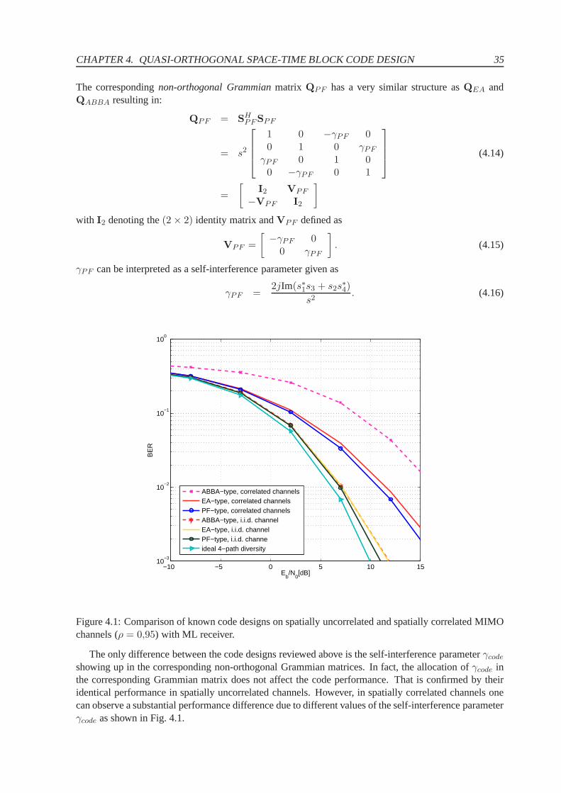
CHAPTER 4. QUASI-ORTHOGONAL SPACE-TIME BLOCK CODE DESIGN 35
The correspondingnon-orthogonal Grammianmatrix QPF has a very similar structure asQEA andQABBA resulting in:
QPF = SHPFSPF
= s2
1 0 −γPF 00 1 0 γPF
γPF 0 1 00 −γPF 0 1
(4.14)
=
[
I2 VPF
−VPF I2
]
with I2 denoting the(2 × 2) identity matrix andVPF defined as
VPF =
[
−γPF 00 γPF
]
. (4.15)
γPF can be interpreted as a self-interference parameter given as
γPF =2jIm(s∗1s3 + s2s
∗4)
s2. (4.16)
−10 −5 0 5 10 1510
−3
10−2
10−1
100
Eb/N
0[dB]
BE
R
ABBA−type, correlated channelsEA−type, correlated channelsPF−type, correlated channelsABBA−type, i.i.d. channelEA−type, i.i.d. channelPF−type, i.i.d. channe�ideal 4−path diversity
Figure 4.1: Comparison of known code designs on spatially uncorrelated and spatially correlated MIMOchannels (ρ = 0,95) with ML receiver.
The only difference between the code designs reviewed aboveis the self-interference parameterγcode
showing up in the corresponding non-orthogonal Grammian matrices. In fact, the allocation ofγcode inthe corresponding Grammian matrix does not affect the code performance. That is confirmed by theiridentical performance in spatially uncorrelated channels. However, in spatially correlated channels onecan observe a substantial performance difference due to different values of the self-interference parameterγcode as shown in Fig. 4.1.
36 4.4. NEW QSTBCS
Example 4.1 Performance of the known QSTBCs applying an ML receiver
In Fig. 4.1 we compared the above explained QSTBCs on spatially uncorrelated as well as on spatiallycorrelated MIMO channels with four transmit antennas and one receive antenna, applying QPSK modu-lation and an ML receiver. We modeled the channel correlation as explained in Chapter 2, Eqn. (2.13).For highly correlated channels withρ = 0,95 the ABBA- type QSTBC shows very poor performance.There is almost10 dB performance loss at BER= 10−2 when compared with i.i.d. channels and about5 dB loss when compared with a PF-type QSTBC, that shows the best performance on highly correlatedMIMO channels. The BER curve named ideal four-path diversity corresponds to an ideal four-path datatransmission assumingγ = 0.
4.4 New QSTBCs
4.4.1 New QSTBCs Obtained by Linear Transformations
Although similar in appearance, the codes (4.3), (4.8), and(4.13) show quite different behavior on par-ticular channels. Thus the question arose how many QSTBCs exist which are equivalent, and are certaincodes optimal for particular channels. Although the first question of how many codes exist is ratherdifficult to answer, we will show in the next section by working out the concept of the equivalent virtualchannel matrix that there are just a few code types withdifferent behavior. This is due to the fact thatvarious QSTBCs can be translated into each other by linear transformations.We consider the following linear transformations on a givenQSTBC:
1. The first transformation of a given code matrix permutes rows and columns in a code matrix. Thisis performed by the application of an elementary permutation matrix or by a concatenation ofseveral elementary permutation matrices. An elementary permutation matrixPij is anN × Nmatrix with ones at its diagonal and zeros at all off-diagonal positions with the exceptionpii =pjj = 0, butpij andpji = 1. E.g., the matrix
P34 =
1 0 0 00 1 0 00 0 0 10 0 1 0
(4.17)
is a permutation matrix that changes the third and the fourthrow or the third and the fourth columnof anN × N matrixS, if P34 multipliesS from the left or from the right.
Applying the permutation matrix to a code matrix either the columns no. i andj are switched(corresponding to switching antennai andj), if we multiply Pij from the right hand side, getting
Snew = SPij, (4.18)
or the rows no.i andj of the code matrixS are switched (which is equivalent to changing thetemporal order of the symbol vector sequence), if we multiply Pij from the left hand side, resultingin:
S′new = PijS. (4.19)
Applying a permutation matrixPij to a symbol vectors the two elements ofs at positioni andjare switched.
CHAPTER 4. QUASI-ORTHOGONAL SPACE-TIME BLOCK CODE DESIGN 37
2. A second class of linear transformations changes the signof either a column or a row of the originalmatrix S. This can be performed by multiplyingS with a diagonal matrixIi which has only+1values at its diagonal entries except at thei−th diagonal position it has a−1. Depending on leftor right multiplication ofIi to the code matrixS, such a matrix can either change the sign of thecolumn No.i with
Ssign = SIi (4.20)
or the sign of thei-th row ofS:S′
sign = IiS. (4.21)
Applying the matrixIi to a symbol vectors the sign of thei−th elementsi is flipped.
3. Similarly to the previous sign inverting transformation, an operatorI∗i (non-multiplicativ) can beapplied to change the entries of column no.i or the entries of the rows no.j to their conjugatecomplex values.
Note that all of these elementary operations are easily performed without essential hardware or soft-ware complexity. Applying one or several of such operationsTi on a given codeword matrix, new codesare generated. In the following we consider transformations of the type:
Snew = [T2C [T1s]]T3. (4.22)
Heres is the set of symbols (for example{s1,s2,s3,s4}) generating the space-time code matrixS. Apermutation matrixT1 may change the ordering of the symbols. The linear code mapping functionC
maps the vectorT1s into a space-time code matrix by repeating the symbols N times in each row in adifferent order. The symbols are placed in such a way that allsymbols appear once in each row and oncein each column. The linear transformationT2 may permute the rows ofC, or may change the entirerows to their conjugate complex values, and/or may reverse the sign of some rows ofC. Finally,T3 maypermute the columns and/or may reverse the sign of some columns.To generate a new quasi-orthogonal space-time code matrixS, the linear transformations described abovemust be applied in such a way, that the new code also fulfills the constraints given in Definition (4.1).Note that all of these linear transformations (4.22) areunitary, i.e., energy preserving. Therefore someessential properties like the trace value of all these codes, remain unchanged.With these linear transformations discussed above the already known code types (4.3), (4.8), and (4.13)can be transformed into each other, and new code variants canbe obtained. This will be illustrated bythe following examples.
Example 4.2 ABBA-type QSTBC obtained by Linear Transformations of the EA-type QSTBC
Let us start with the EA code given in (4.3) Applying a linear transformation (4.19) we can permute the3rd row with the 4th row ofSEA to:
Snew = P34SEA
=
1 0 0 00 1 0 00 0 0 10 0 1 0
s1 s2 s3 s4
−s∗2 s∗1 −s∗4 s∗3−s∗3 −s∗4 s∗1 s∗2
s4 −s3 −s2 s1
=
s1 s2 s3 s4
−s∗2 s∗1 −s∗4 s∗3s4 −s3 −s2 s1
−s∗3 −s∗4 s∗1 s∗2
(4.23)
38 4.4. NEW QSTBCS
whereP34 is the permutation matrix that permutes the 3rd row and the 4th row of SEA. MultiplyingSnew with P34 from the right hand sinde, the 3rd column ofSnew is permuted with the 4th columnresulting in
S′new = SnewP34 =
s1 s2 s4 s3
−s∗2 s∗1 s∗3 −s∗4s4 −s3 s1 −s2
−s∗3 −s∗4 s∗2 s∗1
. (4.24)
Changing the sign of the 2nd column and the 4th row leads to an ABBA-type QSTBC defined in (4.8):
SEAnew = I2[S′newI2]=SABBA(S12 ,S34)=
[
S12 S34
S34 S12
]
=
s1 −s2 s4 s3
−s∗2 −s∗1 s∗3 −s∗4s4 s3 s1 −s2
s∗3 −s∗4 −s∗2 −s∗1
. (4.25)
TheIi are diagonal matrices defined in (4.20) and (4.21), respectively, andS12 andS34 are the Alamouti-type (2 × 2) STBCs (see Appendix A) with differently arranged symbols. The corresponding non-orthogonal Grammian matrixQ has the same structure asQABBA given in (4.9) with the self-interferenceparameterγEA already given in (4.11):
SEAnewSHEAnew
= s2
1 0 γEA 00 1 0 γEA
γEA 0 0 00 γEA 0 1
.
Example 4.3 EA-type QSTBC obtained by Linear Transformations of the ABBA-type QSTBC
In a similar way as shown in the previous example, we can applythe linear transformation (4.22) on theABBA code (4.8) to obtain a new QSTBC. The new code matrix is generated by applying the followinglinear transformations toSABBA
[
I4[P34SABBA
]
P12]I1 = SABBAnew , (4.26)
whereP34 denotes the permutation matrix that permutes the 3rd and the4th row of the ABBA codematrix, P12 changes the 1st and the 2nd column of the code matrix in brackets , the diagonal matrixI4 changes the sign in the 4th row, and the diagonal matrixI1 changes the sign of the 1st column thecorresponding matrix. Finally, the new code matrix has the structure of the EA-type QSTBC with
SABBAnew = SEA(S12 ,S34) =
[
S12 S34
−S∗34 S∗
12
]
=
s2 −s1 s3 s4
s∗1 s∗2 −s∗4 s∗3−s∗3 −s∗4 s∗2 −s∗1
s4 −s3 s1 s2
.
This linear transformation leads to a new QSTBC with a non-orthogonal Grammian matrixQ similar tothe EA code (4.4)
SABBAnewSHABBAnew
= s2
1 0 0 −γnew
0 1 γnew 00 γnew 1 0
−γnew 0 0 1
.
CHAPTER 4. QUASI-ORTHOGONAL SPACE-TIME BLOCK CODE DESIGN 39
with the self-interference parameter
γnew =2Re(s1s
∗3 + s2s
∗4)
s2. (4.27)
As has been demonstrated by these two examples, the linear transformations can lead to differentpositions of the interference parameterγ in the corresponding Grammian matrix. However, we willshow that the positions of the interference parameter essentially do not influence the performance of theQSTBC, but rather the value of the interference parameterγ effects the code performance.In [48] some other examples of QSTBCs obtained by permutations of rows and/or columns of a givencode matrix can be found.
4.5 Equivalent Virtual Channel Matrix (EVCM)
As will be shown in this section, an important characteristic of QSTBCs is their unique equivalent, highlystructured, virtual MIMO channel matrixHv with the following property:
Definition 4.2 The equivalent virtual channel matrixHv is a matrix that satisfiesHHv Hv =
∑N1 |hi|2G,
whereG is a sparse matrix with ones on its main diagonal, having at least N2/2 zero entries at off-diagonal positions and its remaining (self-interference)entries being bounded in magnitude by1.
The EVCM has a very similar structure as the code matrixS of the underlying QSTBC.
Example 4.4 Construction of the EVCM
Let us consider a QSTBC denoted byS, e.gSEA from (4.3), and an(4×1) frequency flat MISO channel.Then we obtain
r = Sh + n, (4.28)
as already shown in (3.39) wherer denotes the vector of four temporally successive signal samples at thereceive antenna. The channel coefficients are denoted byh = [h1, h2, h3, h4]
T , andn = [n1, n2, n3, n4]T
is the noise vector. Assuming a single receive antenna and the code matrixSEA given in (4.3) the re-ceived signals within four successive time slots are given as:
r1 = s1h1 + s2h2 + s3h3 + s4h4 + n1
r2 = s∗2h1 − s∗1h2 + s∗4h3 − s∗3h4 + n2
r3 = s∗3h1 + s∗4h2 − s∗1h3 − s∗2h4 + n3
r4 = s4h1 − s3h2 − s2h3 + s1h4 + n4. (4.29)
If the second and the third row of the code matrixSEA is complex conjugated, then the modified receivedsignal vectory can be written as
y =
r1
r∗2r∗3r4
= Hvs + n, (4.30)
with
y1 = r1, n1 = n1
y2 = r∗2, n2 = n∗2
y3 = r∗3, n3 = n∗3
y4 = r4, n4 = n4,
40 4.6. RECEIVER ALGORITHMS FOR QSTBCS
and the virtual equivalent (4 × 4) channel matrixHv given as
Hv =
h1 h2 h3 h4
h∗2 −h∗
1 h∗4 −h∗
3
h∗3 h∗
4 −h∗1 −h∗
2
h4 −h3 −h2 h1
. (4.31)
In this caseHv can be interpreted as an equivalent, highly structured, virtual (4 × 4) MIMO channelmatrix (EVCM), replacing the(4 × 1) channel vectorh.
In this way, the QSTBC pretends a virtual, specificallystructured (4 × 4) MIMO channel with fourtransmit and four virtual receive antennas. This EVCM simplifies the analysis of the QSTBCs as will beshown in the next chapter.
4.6 Receiver Algorithms for QSTBCs
4.6.1 Maximum Ratio Combining
The simplest way to decode a QSTBCs is to apply a simple maximum ratio combining technique. Amaximum ratio combining (MRC) of the modified received signal vectory can be done in a very simpleway by multiplyingy with HH
v3. Then we obtain a new decision vectorz as
z = HHv y = HH
v Hvs + HHv n
= Gs + Hvn, (4.32)
with thenon-orthogonal GrammianmatrixG = HHv Hv. G is asparsematrix with the real-valued gain
factorh2 at its main diagonal and a self-interference factorX at some off-diagonal positions. This self-interference factor can be real or purely imaginary, as we will explain later. This fact is very importantfor the efficient decoding algorithm of the QSTBCs.For the EA-type QSTBCs, thenon-orthogonal GrammianmatrixG has following form
G = HvHHv = HH
v Hv = h2
1 0 0 X0 1 −X 00 −X 1 0
X 0 0 1
(4.33)
with
h2 = |h1|2 + |h2|2 + |h3|2 + |h4|2, (4.34)
and
X =2Re(h1h
∗4 − h2h
∗3)
h2.
Note, that in case of orthogonal STBCs the corresponding Grammian matrixG is strictly diagonal(as it has been shown for the Alamouti scheme). Therefore, OSTBCs have an important advantage indecoding, that comes from the fact that the inverse of the Grammian matrixG is proportional to theidentity matrix. This means that the MRC receiver degenerates to a low-complexity ZF receiver withs = 1/h2HHy = s + nZF and behaves exactly as an otherwise high-complex ML receiver.
3In literature, the operationHHv is often denoted as matched filtering (MF). Through this thesis we will denote it as a MRC.
CHAPTER 4. QUASI-ORTHOGONAL SPACE-TIME BLOCK CODE DESIGN 41
Returning to ournon-orthogonal Grammianmatrix (4.33) corresponding to the MRC receiver oper-ating according to (4.32), we find that decoding can be performed not one by one symbol but by splittingup the decision vectorz into the subsetsz1 andz4, andz2 andz3. Due to the symmetry in (4.33), af-ter MRC, the 4-input / 4-output system can be perfectly decoupled into sets of two 2-input / 2-outputsystems. This can be seen by writing (4.32) explicitly as
z = h2
s1 + Xs4
s2 − Xs3
s3 − Xs2
s4 + Xs1
+ HHv n (4.35)
and by grouping the entries ofz in two pairs
[
z1
z4
]
= h2
[
1 XX 1
] [
s1
s4
]
+
[
n1
n4
]
[
z2
z3
]
= h2
[
1 −X−X 1
] [
s2
s3
]
+
[
n2
n3
]
, (4.36)
where theni i = 1, · · · , 4 are the receive noise terms after MRC. It is important to emphasize that thetwo pairs of symbols in equation (4.35) are completely decoupled. As will be shown later, this leads tocomplexity and computation reduction at the receiver.After MRC an additional decoding step is required in order toretrieve the input signal. Different strate-gies can be applied at this final step, from optimal Maximum Likelihood detection to ZF or MMSEequalization (as will be described in the next section). Specific decoding solution for QSTBCs have beenderived in [44] and [49].
4.6.2 Maximum Likelihood (ML) Receiver
The ML detector is optimal in the sense of minimum error probability when all transmitted data vectorsare equally probable. However, this optimality is obtainedat the cost of an exponentially increasing com-putational complexity depending on the symbol constellation size and the number of transmit antennas.In general, the ML detector selects that signal vectors that minimizes the distanceDML1
(s) betweenthe receive vectory and all possible undisturbed output vectorsHvsi, wheresi stands for all possibletransmit vectors. For a specific transmit vectors we obtain
DML1(s) = ||y − Hvs||2 = sHGs− 2Re(yHvs) + ||y||2. (4.37)
Considering a QPSK modulation we have to take into account44 = 256 symbol vectorssi to find thebest metricDML1
(s).Using QSTBCs it is possible to reduce the decoding complexity of the ML- detector applying MRC(4.32) toy before applying ML detection. In fact, the ML detection is now applied toz instead toy.The benefit of this approach is that the MRC partly decouples the symbols. E.g for the EA-code (4.3)the symbol pair{s1, s4} is decoupled from{s2, s3}. Consequently, the ML algorithm has to be appliedtwice to search over both signal pairs but only over a reducedset of42 = 16 symbol pairs. The newdistance metric equivalent to (4.37) can be written as4
DML2(s) = (z − Gs)HG−1(z − Gs). (4.38)
4A proof can be found in the Appendix C.
42 4.6. RECEIVER ALGORITHMS FOR QSTBCS
Exploiting the sparse structure of the non-orthogonal Grammian matrix and following (4.36), for theEA-type QSTBC, equation (4.38) results in
DML2(s) =
z1
z2
z3
z4
−
s1 + Xs4
s2 − Xs3
s3 − Xs2
s4 + Xs1
H
1
1 − X2
1 0 0 −X0 1 X 00 X 1 0
−X 0 0 1
·
z1
z2
z3
z4
−
s1 + Xs4
s2 − Xs3
s3 − Xs2
s4 + Xs1
=1
1 − X2
[
z1 − h2(s1 + Xs4)z4 − h2(s4 + Xs1)
]H [1 −X
−X 1
] [
z1 − h2(s1 + Xs4)z4 − h2(s4 + Xs1)
]
+1
1 − X2
[
z2 − h2(s2 − Xs3)z3 − h2(s3 − Xs2)
]H [1 XX 1
] [
z2 − h2(s2 − Xs3)z3 − h2(s3 − Xs2)
]
= DML(s1, s4) + DML(s2, s3), (4.39)
with
DML(s1, s4) =1
1 − X2
(
|z1 − h2(s1 + Xs4)|2 + |z4 − h2(s4 + Xs1)|2
− 2XRe{[z1 − h2(s1 + Xs4)][z∗4 − h2(s∗4 + Xs∗1)]}
)
(4.40)
and
DML(s2, s3) =1
1 − X2
(
|z2 − h2(s2 − Xs3)|2 + |z3 − h2(s3 − Xs2)|2
+ 2XRe{[z2 − h2(s2 − Xs3)][z∗3 − h2(s∗3 − Xs∗2)]}
)
. (4.41)
The pair {s1, s4} is detected by minimizingDML(s1, s4) over all symbol combinationss1 and s4
transmitted over transmit antennant1 and nt4 and symbol pair{s2, s3} is detected by minimizingDML(s2, s3) over all symbol combinationss2 and s3 transmitted over transmit antennant2 and nt3 .Finally, both search algorithms (4.37) and (4.38) give the whole estimated transmit vectors [47], [52],[53]. Applying (4.38) or (4.40) and (4.41) respectively, the ML algorithm only searches over a reducedset of42 = 16 symbol pairs. In Fig. 4.2 the performance of QSTBC applying aML receiver is shown.
4.6.3 Linear Receivers
Linear receivers (Zero Forcing (ZF) and Mean Squared Error(MMSE) receiver) can reduce the decodingcomplexity but they typically suffer from noise enhancement. Linear detection can be described by
s = (HHv Hv + µI)−1z (4.42)
whereµ = 0 for the ZF receiver andµ = σ2n for the MMSE receiver. The MMSE receiver behaves
similar to the ZF receiver, however with an additional term in the matrix inverse proportional to the noisevariance. In practice it can be difficult to obtain correct values ofσ2
n. But only for correct values a smallimprovement compared to the ZF receiver can be obtained. Therefore, the MMSE technique is not usedin practice and will be not discussed in this thesis furthermore.
CHAPTER 4. QUASI-ORTHOGONAL SPACE-TIME BLOCK CODE DESIGN 43
A ZF receiver is highly appreciated for its low complexity. For large signal alphabets this can beof great advantage, whereas for small signal alphabets the ML receiver can compete in complexity. ZFdecoding of QSTBCs separates the received signal into its components by
s =(
HvHHv
)−1z = s +
(
HvHHv
)−1Hv
H n = s + n. (4.43)
The ZF receiver decouples the channel matrix intont parallel scalar channels with additive noise. Thenoise is enhanced by the factor(HvH
Hv )−1 and furthermore, the noise is correlated across the channels
and contains signal components ofs (self-interference) due to the self-interference parameter X. Thecorrelation of the resulting noise samples is given by
E[nnH ] = σ2n
(
HvHHv
)−1= σ2
nG−1
=σ2
n
h2(1 − X2)
1 0 0 −X0 1 X 00 X 1 0
−X 0 0 1
. (4.44)
In the final detection, the ZF receiver decodes each stream independently ignoring noise correlation andself-interference. The decision about which symbols have been transmitted are then taken using a detec-tor that associates to each term ofs the nearest symbol belonging to the constellation of the transmittedsymbols.The resulting estimated signal vector is denoted ass. The ZF receiver reduces the decoding complexity,but the receiver is sub-optimal and leads to a significant performance degradation. However, if the CSIinformation is available at the transmitter, the self-interference can be compensated and the ZF receivercan perform as well as the ML receiver, as we will show in next chapter.
Since we know the covariance matrix of the filtered noise, theBER of QSTBC for ZF receiver is easyto calculate as has been shown in [47]. Thei-th diagonal element of the covariance matrix denotes thevariance of the modified noisen:
σ2n =
σ2ni
h2(1 − X2), 1 ≤ i ≤ 4 (4.45)
Considering (4.45), the BER for QSTBC is obtained5
BERZF = Eh2,X
{
Q(√
h2(1 − X2)
σ2n
)}
, (4.46)
where the expectation value is computed with respect to the channel gainh2 and the self-interferenceparameterX contained inG. The statistical properties ofh2 andX will be discussed in detail in Section4.7.5.From the above analytical result it is obvious, that the power of the filtered noise increases with increas-ing X. Additionally, the correlation between the noise samplesni also increases withX leading to aperformance gap compared with the results obtained by the MLreceiver [52]. The performance of theQSTBC applying a low complexity ZF receiver is also shown in Fig. 4.2.
Example 4.5 Performance of the EA-type QSTBC for different receiver types
In Fig. 4.2 we illustrate the BER performance of the EA-type QSTBC given in (4.3) for different receivertypes in case of i.i.d. Rayleigh fading averaged over 10.000channel realizations. We apply an ML
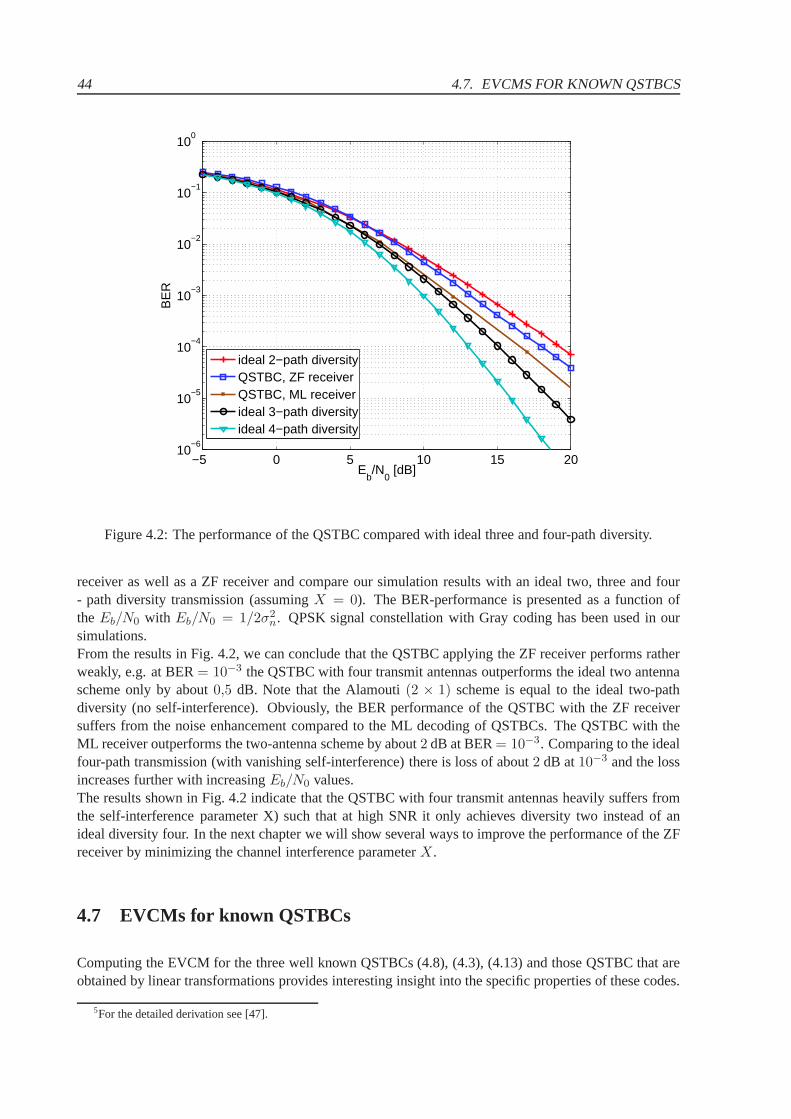
44 4.7. EVCMS FOR KNOWN QSTBCS
−5 0 5 10 15 2010
−6
10−5
10−4
10−3
10−2
10−1
100
Eb/N
0 [dB]
BE
R
ideal 2−path diversityQSTBC, ZF receiverQSTBC, ML receiverideal 3−path diversityideal 4−path diversity
Figure 4.2: The performance of the QSTBC compared with idealthree and four-path diversity.
receiver as well as a ZF receiver and compare our simulation results with an ideal two, three and four- path diversity transmission (assumingX = 0). The BER-performance is presented as a function ofthe Eb/N0 with Eb/N0 = 1/2σ2
n. QPSK signal constellation with Gray coding has been used inoursimulations.From the results in Fig. 4.2, we can conclude that the QSTBC applying the ZF receiver performs ratherweakly, e.g. at BER= 10−3 the QSTBC with four transmit antennas outperforms the idealtwo antennascheme only by about0,5 dB. Note that the Alamouti(2 × 1) scheme is equal to the ideal two-pathdiversity (no self-interference). Obviously, the BER performance of the QSTBC with the ZF receiversuffers from the noise enhancement compared to the ML decoding of QSTBCs. The QSTBC with theML receiver outperforms the two-antenna scheme by about2 dB at BER= 10−3. Comparing to the idealfour-path transmission (with vanishing self-interference) there is loss of about2 dB at10−3 and the lossincreases further with increasingEb/N0 values.The results shown in Fig. 4.2 indicate that the QSTBC with four transmit antennas heavily suffers fromthe self-interference parameter X) such that at high SNR it only achieves diversity two instead of anideal diversity four. In the next chapter we will show several ways to improve the performance of the ZFreceiver by minimizing the channel interference parameterX.
4.7 EVCMs for known QSTBCs
Computing the EVCM for the three well known QSTBCs (4.8), (4.3), (4.13) and those QSTBC that areobtained by linear transformations provides interesting insight into the specific properties of these codes.
5For the detailed derivation see [47].
CHAPTER 4. QUASI-ORTHOGONAL SPACE-TIME BLOCK CODE DESIGN 45
In the following,h2 denotes the overalchannel gain(also called fading factor) with
h2 = |h1|2 + |h2|2 + |h3|2 + |h4|2
indicating a potential system diversity order of four in allcases.
4.7.1 EVCM for the Jafarkhani Code
As already shown in Example 4.4, by changing the second and third element of the receive vector thatstems from the EA-code matrixSEA into their conjugate complex-values, the EVCM for the EA-codecan be derived. This virtual channel matrixHvEA
shows the same sub-block structure as the code matrixSEA in (4.3) and results in
HvEA=
[
Hv12Hv34
H∗v34
−H∗v12
]
=
h1 h2 h3 h4
h∗2 −h∗
1 h∗4 −h∗
3
h∗3 h∗
4 −h∗1 −h∗
2
h4 −h3 −h2 h1
. (4.47)
The corresponding non-orthogonal Grammian matrixGEA results in:
GEA = HHvEA
HvEA
= h2
1 0 0 XEA
0 1 −XEA 00 −XEA 1 0
XEA 0 0 1
(4.48)
= h2
[
I2 WE
−WE I2
]
,
whereh2 is the channel gain factor given in (4.34),I2 is the(2 × 2) identity matrix,WEA is defined as
WEA =
[
0 XEA
−XEA 0
]
, (4.49)
andXEA is a channel dependent self-interference parameter resulting in
XEA =2Re(h1h
∗4 − h2h
∗3)
h2. (4.50)
4.7.2 EVCM for the ABBA Code
Similarly to Example 4.4, the second and the fourth element of the receive vector are complex conjugated.Then we obtain the equivalent virtual MIMO channel matrix for the ABBA Code (4.8):
HvABBA=
[
Hv12Hv34
Hv34Hv12
]
=
h1 h2 h3 h4
h∗2 −h∗
1 h∗4 −h∗
3
h3 h4 h1 h2
h∗4 −h∗
3 h∗2 −h∗
1
. (4.51)
Multiplying (4.51) with its Hermitian conjugate leads to the Grammian matrixGABBA:
GABBA = HHvABBA
HvABBA
= h2
1 0 XA 00 1 0 XA
XA 0 1 00 XA 0 1
(4.52)
= h2
[
I2 WA
WA I2
]
,
46 4.7. EVCMS FOR KNOWN QSTBCS
whereh2 is the channel gain given in (4.34),I2 is the(2 × 2) identity matrix,WA defined as
WABBA =
[
XA 00 XA
]
(4.53)
andXA is a channel dependent self-interference parameter resulting in:
XA =2Re(h1h
∗3 + h2h
∗4)
h2. (4.54)
4.7.3 EVCM for the Papadias-Foschini Code
A third version of an EVCM is obtained from the Papadias-Foschini code (4.13). This EVCM does nothave a sub-block structure as the EVCMs discussed above:
HvPF=
h1 h2 h3 h4
−h∗2 h∗
1 −h∗4 h∗
3
−h3 h4 h1 −h2
−h∗4 −h∗
3 h∗2 h∗
1
. (4.55)
The Grammian matrixGPF is obtained as
GPF = HHvPF
HvPF
= h2
1 0 XPF 00 1 0 −XPF
−XPF 0 1 00 XPF 0 1
(4.56)
= h2
[
I2 WPF
−WPF I2
]
whereh2 is the channel gain given in (4.34),I2 is the(2 × 2) identity matrix,WPF is defined as
WPF =
[
XPF 00 −XPF
]
(4.57)
with the channel dependent self-interference parameterXPF :
XPF =2jIm(h∗
1h3 + h2h∗4)
h2. (4.58)
4.7.4 Other EVCMs with Channel Independent Diagonalization of G
The main focus in the design of useful QSTBCs is the Grammian matrixG that is of essential importancein decoding the QSTBCs. Following Definition 4.1 and Definition 4.2, the Grammian matrix of eachQSTBC for four transmit antennas can be written in the following general way:
GQSTBC = HHv Hv = HvH
Hv
= h2
[
I2 XcodeWl
XcodeWl I2
]
l = 1,2 (4.59)
CHAPTER 4. QUASI-ORTHOGONAL SPACE-TIME BLOCK CODE DESIGN 47
with Wl beeing either
W1 =
[
±1 00 ±1
]
, or W2 =
[
0 ±1±1 0
]
. (4.60)
The Grammian matrixG should approximate a scaled identity-matrix as far as possible to achievefull diversity and optimum BER performance. IfG is a scaled identity matrix, we have an orthogonalSTBC and we could use a simple linear matrix multiplication of the modified received vectory byHH
v todecouple the vector component ofs perfectly and to obtain full diversity orderd = 4. Otherwise,Xcode
leads to a partial interference between symbol pairs. This means,X should beas small as possible. As(4.46) indicates, we can achieve full diversityd = 4, if X can be made zero. In the next chapter we willshow several ways to minimize the self-interference parameter X.
A nice property of the Grammian matrixG shown in (4.59) is the fact that it can be diagonalized byΛ = DT GD with a channelindependenteigenmatrixD [45], [52] given as
D =1√2
[
I2 Ji
Ji I2
]
, (4.61)
consisting of the(2 × 2) identity matrixI2, andJi resulting either as
J1 =
[
0 ±1±1 0
]
or J2 =
[
±1 00 ±1
]
(4.62)
depending on which code design is considered.J1 results in case of the EA-type QSTBCs andJ2 in caseof the ABBA-type or the PF-type QSTBCs.The diagonal matrixΛ consists of two pairs of eigenvalues with :
λ1 = λ2 = h2(1 + X)
λ3 = λ4 = h2(1 − X). (4.63)
Obviously, these eigenvalues depend on the channel parameters. In case ofX = 0 all eigenvalues areequal.
4.7.5 Statistical Properties of the Channel Dependent Self-Interference Parameter
Since the self-interference parameterX is the most important parameter of a QSTBC with respect to di-versity order and BER performance, in the following we will discuss its statistical properties at Rayleighfading channels in detail. If the channel coefficientshi are complex i.i.d. Gaussian distributed randomvariables, then the probability density function (pdf) ofX can be easily derived. Starting e.g. withXEA
in (4.50) given as:
XEA =2Re(h1h
∗4 − h2h
∗3)
h2(4.64)
we can calculateXEA + 1 as [47]
XEA + 1 =|h1 + h4|2 + |h2 − h3|2
|h1|2 + |h2|2 + |h3|2 + |h4|2. (4.65)
Sincehi are i.i.d. complex-valued Gaussian distributed variables, the variablesh1 + h4 andh2 − h3 arealso complex Gaussian distributed and independent of each other. Defining a linear orthogonal coordinatetransformation
u = (h1 + h4)/√
2, v = (h2 − h3)/√
2,
u′ = (h1 − h4)/√
2, v′ = (h2 + h3)/√
2, (4.66)
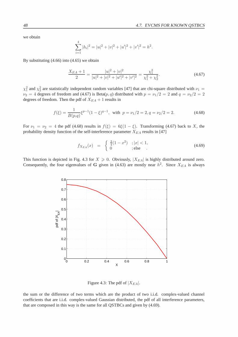
48 4.7. EVCMS FOR KNOWN QSTBCS
we obtain4∑
i=1
|hi|2 = |u|2 + |v|2 + |u′|2 + |v′|2 = h2.
By substituting (4.66) into (4.65) we obtain
XEA + 1
2=
|u|2 + |v|2|u|2 + |v|2 + |u′|2 + |v′|2 =
χ21
χ21 + χ2
2
. (4.67)
χ21 andχ2
2 are statistically independent random variables [47] that are chi-square distributed withν1 =ν2 = 4 degrees of freedom and (4.67) is Beta(p, q) distributed withp = ν1/2 = 2 andq = ν2/2 = 2degrees of freedom. Then the pdf ofXEA + 1 results in
f(ξ) =1
B(p,q)ξp−1(1 − ξ)q−1, with p = ν1/2 = 2, q = ν2/2 = 2. (4.68)
For ν1 = ν2 = 4 the pdf (4.68) results inf(ξ) = 6ξ(1 − ξ). Transforming (4.67) back toX, theprobability density function of the self-interference parameterXEA results in [47]
fXEA(x) =
{
34(1 − x2) ; |x| < 1,0 ; else .
(4.69)
This function is depicted in Fig. 4.3 forX > 0. Obviously, |XEA| is highly distributed around zero.Consequently, the four eigenvalues ofG given in (4.63) are mostly nearh2. SinceXEA is always
0 0.2 0.4 0.6 0.8 10
0.1
0.2
0.3
0.4
0.5
0.6
0.7
0.8
X
pdf o
f |X
EA|
Figure 4.3: The pdf of|XEA|.
the sum or the difference of two terms which are the product oftwo i.i.d. complex-valued channelcoefficients that are i.i.d. complex-valued Gaussian distributed, the pdf of all interference parameters,that are composed in this way is the same for all QSTBCs and given by (4.69).
CHAPTER 4. QUASI-ORTHOGONAL SPACE-TIME BLOCK CODE DESIGN 49
4.7.6 Common Properties of the Equivalent Virtual Channel Matrices Corresponding toQSTBCs
Let us now summarize the main properties of the EVCMs and their Grammian matricesG for fourtransmit antennas:
1. Any virtual MIMO channel matrixHv has a structure very similar to the corresponding quasi-orthogonal code matrixS.
2. Working out linear transformations onS in such a way that the sparse structure ofG with onlyone off-diagonal self-interference parameterX is maintained, these transformations may changethevalue of X.
3. The self-interference parameterX indicates the non-orthogonality of the code. The closerX is tozero, the closer is the quasi orthogonal code to an orthogonal code withG = h2I.
4. |X| is bounded by1, and thus the eigenvalues ofG are in the range ofh2[0,2].
5. In all (4×4) EVCMs, the Grammian matrixG has two pairs of eigenvalues with valuesh2(1±X).Due to the channel gain given in (4.34), QSTBCs provide potentially full diversity, if X 6= 1.
6. SinceX is the only term that changes its value with the constrained linear transformations,onlythe values ofX (but not the eigenvectors ofHv) depend on the particular channel realization, andthus determine the BER performance of the code.
7. By an appropriate code design,X can be designed to be either purely real-valued or purelyimaginary-valued (as will be shown in Section (4.7.7.1)).
The number of distinct QSTBCs is not easy to find. However, thenumber ofusefulcodes that showa distinct behavior on a given wireless MIMO channel can be easily derived. Although many lineartransformations exist which lead to different QSTBCs, someconstraints are necessary to achieveusefulQSTBC codes in the case of four transmit antennas. Therefore, we propose a definition ofusefulQSTBCsconsidering a QSTBC design with respect to their corresponding EVCMs:
Definition 4.3 AusefulQSTBC of dimensionN×N has an EVCM that satisfiesHvHvH =
∑N1 |hi|2G
with G being a sparse matrix with ones on its main diagonal, having at leastN2/2 zero entries at off-diagonal positions and its remaining entries being boundedin magnitude by1.
With the Definition (4.3) and the design rules proposed in theprevious sections, we can reduce thelarge number of different QSTBCs to 12usefulcode types. In the next section we will present these 12useful code types and we will discuss their BER performance.
4.7.7 Useful QSTBC Types
In previous sections, we have required, that by linear transformations of the QSTBCs the sparse struc-ture of the GrammianG matrix is preserved and only the value of the interference parameterX maybe changed. By these constraints, the number of useful QSTBCs that perform differently can be easilycalculated. SinceX is always the real or the imaginary part of the sum or the difference of two complexterms which are the product of two channel coefficients in case of four transmit antennas, only 12 dif-ferent code types exist (we do not count the negative values of X seperately, since these codes have the
50 4.7. EVCMS FOR KNOWN QSTBCS
same BER performance). The 12 distinctX values that can occur with useful QSTBCs are listed below.First, six code types with real-valued self-interference parametersXi are given as:
X1 =2Re(h1h
∗3 + h2h
∗4)
h2
X2 =2Re(h1h
∗3 − h2h
∗4)
h2
X3 =2Re(h1h
∗2 + h3h
∗4)
h2(4.70)
X4 =2Re(h1h
∗2 − h3h
∗4)
h2
X5 =2Re(h1h
∗4 + h2h
∗3)
h2
X6 =2Re(h1h
∗4 − h2h
∗3)
h2.
Additionally, we can get six code types with purely imaginary-valuedXi given as:
X7 =2jIm(h1h
∗3 + h2h
∗4)
h2
X8 =2jIm(h1h
∗3 − h2h
∗4)
h2
X9 =2jIm(h1h
∗2 + h3h
∗4)
h2(4.71)
X10 =2jIm(h1h
∗2 − h3h
∗4)
h2
X11 =2jIm(h1h
∗4 + h2h
∗3)
h2
X12 =2jIm(h1h
∗4 − h2h
∗3)
h2.
The corresponding QSTBCs can be found by starting with an arbitrary QSTBC and applying appro-priate linear transformations as described in Section 4.4.1. Given a wireless channel, these 12 possiblevariants ofX indicate whether the obtained code is close to an orthogonalcode or not. A detailedanalysis of these codes is given in Section 4.7.8.
4.7.7.1 QSTBCs with real and purely imaginary-valued self-interference parameters
In Appendix B we have listed examples of useful QSTBCs matricesS. The subscripts of the QSTBCspresented there correspond to the subscripts of the channeldependent parametersXi given in (4.70)and (4.71). By linear transformations many different variants of the QSTBCs with the same channeldependent self-interference parameterX can be obtained. In fact, we distinguish between two classesofQSTBCs according to their interference parameterX: Codes with real-valued self-interference parame-tersXi and codes with imaginary-valued self-interference parametersXi.Studying these different codes we have found one additionalinteresting property of QSTBCs:
Conjecture 4.1 If the QSTBC signal matrix has a block-structure obtained bytwo different(2 × 2)Alamouti-like matrices and their conjugate complex and/ortheir negative variants, the values ofX arealways real-valued. Otherwise,X is purely imaginary.
CHAPTER 4. QUASI-ORTHOGONAL SPACE-TIME BLOCK CODE DESIGN 51
We corroborate this conjecture by an example.
Example 4.6 QSTBCs with real-valued channel dependent self-interference parameterX.
We start with the ABBA-type QSTBC (4.8)
QSTBC =
[
S1 S2
S2 S1
]
with the EVCM Hv =
[
Hv1 Hv2
Hv2 Hv1
]
, (4.72)
whereHv1andHv2
are(2 × 2) EVCMs with Alamouti-like structure. e.g.
Hv1=
[
h1 h2
−h∗2 h∗
1
]
, Hv2=
[
h3 h4
−h∗4 h∗
3
]
. (4.73)
The Grammian matrix ofHv can be calculated as
G = HvHHv = HH
v Hv
=
[
Hv1Hv2
Hv2Hv1
]
·[
Hv1Hv2
Hv2Hv1
]H
=
[
Hv1Hv2
Hv2Hv1
]
·[
HHv1
HHv2
HHv2
HHv1
]
=
[
Hv1HH
v1+ Hv2
HHv2
Hv1HH
v2+ Hv2
HHv1
Hv1HH
v2+ Hv2
HHv1
Hv1HH
v1+ Hv2
HHv2
]
. (4.74)
Hv1HH
v1andHv2
HHv2
are real-valued and the corresponding(2 × 2) Grammian matrices are diagonal:
Hv1HH
v1= (|h1|2 + |h2|2)I2 (4.75)
Hv2HH
v2= (|h3|2 + |h4|2)I2. (4.76)
The off-diagonal submatrices of the matrixG show the following structure:
Hv1HH
v2+ Hv2
HHv1
= Hv1HH
v2+ (Hv1
HHv2
)H
= A + AH . (4.77)
From matrix algebra, we know that if a matrixA is a complex-valued matrix, than it follows thatA+AH
is a matrix with real diagonal values (aii + a∗ii = 2Re{aii}). Thus the termHv1HH
v2+ Hv2
HHv1
is a(2 × 2) matrix with real diagonal values:
Hv1HH
v2+ Hv2
HHv1
=
[
h1 h2
−h∗2 h∗
1
]
·[
h3 h4
−h∗4 h∗
3
]H
+
[
h3 h4
−h∗4 h∗
3
]
·[
h1 h2
−h∗2 h∗
1
]H
=
[
h1h∗3 + h2h
∗4 −h1h4 + h2h3
−h∗2h
∗3 + h∗
1h∗4 h∗
2h4 + h∗1h3
]
+
[
h3h∗1 + h4h
∗2 h4h1 − h3h2
h∗3h
∗2 − h∗
4h∗1 h∗
4h2 + h∗3h1
]
=
[
2Re(h1h∗3 + h2h
∗4) 00 2Re(h1h
∗3 + h2h
∗4)
]
. (4.78)
This real diagonal value has been called self-interferenceparameter in the previous section. Thereforeany QSTBC signal matrix with a block structure as the ABBA-type QSTBC, (4.8) has a real-valued self-interference parameterX. In a similar way it can be shown that all QSTBCs with block structure fromthe EA-type QSTBC (4.3) have a real-valued self-interference parameter.
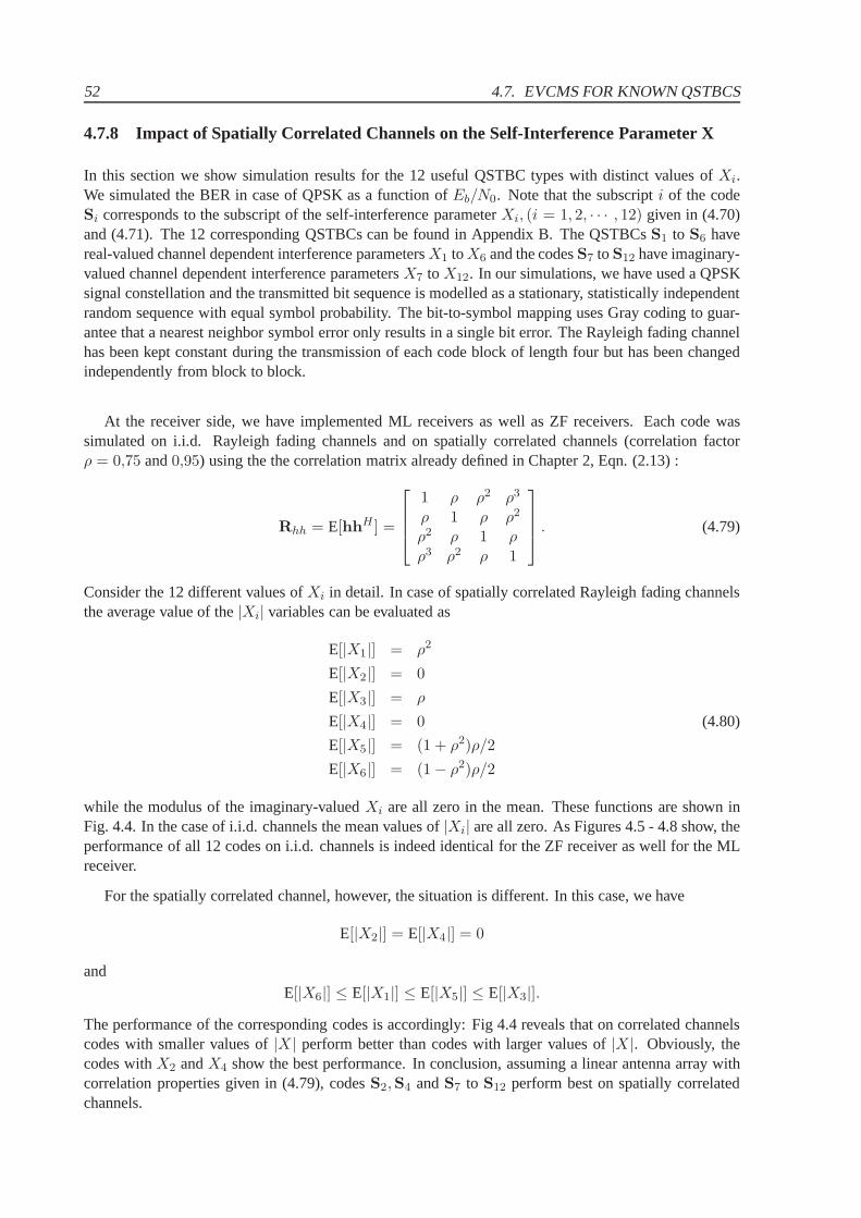
52 4.7. EVCMS FOR KNOWN QSTBCS
4.7.8 Impact of Spatially Correlated Channels on the Self-Interference Parameter X
In this section we show simulation results for the 12 useful QSTBC types with distinct values ofXi.We simulated the BER in case of QPSK as a function ofEb/N0. Note that the subscripti of the codeSi corresponds to the subscript of the self-interference parameterXi, (i = 1, 2, · · · , 12) given in (4.70)and (4.71). The 12 corresponding QSTBCs can be found in Appendix B. The QSTBCsS1 to S6 havereal-valued channel dependent interference parametersX1 toX6 and the codesS7 toS12 have imaginary-valued channel dependent interference parametersX7 to X12. In our simulations, we have used a QPSKsignal constellation and the transmitted bit sequence is modelled as a stationary, statistically independentrandom sequence with equal symbol probability. The bit-to-symbol mapping uses Gray coding to guar-antee that a nearest neighbor symbol error only results in a single bit error. The Rayleigh fading channelhas been kept constant during the transmission of each code block of length four but has been changedindependently from block to block.
At the receiver side, we have implemented ML receivers as well as ZF receivers. Each code wassimulated on i.i.d. Rayleigh fading channels and on spatially correlated channels (correlation factorρ = 0,75 and0,95) using the the correlation matrix already defined in Chapter2, Eqn. (2.13) :
Rhh = E[hhH ] =
1 ρ ρ2 ρ3
ρ 1 ρ ρ2
ρ2 ρ 1 ρρ3 ρ2 ρ 1
. (4.79)
Consider the 12 different values ofXi in detail. In case of spatially correlated Rayleigh fading channelsthe average value of the|Xi| variables can be evaluated as
E[|X1|] = ρ2
E[|X2|] = 0
E[|X3|] = ρ
E[|X4|] = 0 (4.80)
E[|X5|] = (1 + ρ2)ρ/2
E[|X6|] = (1 − ρ2)ρ/2
while the modulus of the imaginary-valuedXi are all zero in the mean. These functions are shown inFig. 4.4. In the case of i.i.d. channels the mean values of|Xi| are all zero. As Figures 4.5 - 4.8 show, theperformance of all 12 codes on i.i.d. channels is indeed identical for the ZF receiver as well for the MLreceiver.
For the spatially correlated channel, however, the situation is different. In this case, we have
E[|X2|] = E[|X4|] = 0
andE[|X6|] ≤ E[|X1|] ≤ E[|X5|] ≤ E[|X3|].
The performance of the corresponding codes is accordingly:Fig 4.4 reveals that on correlated channelscodes with smaller values of|X| perform better than codes with larger values of|X|. Obviously, thecodes withX2 andX4 show the best performance. In conclusion, assuming a linearantenna array withcorrelation properties given in (4.79), codesS2,S4 andS7 to S12 perform best on spatially correlatedchannels.
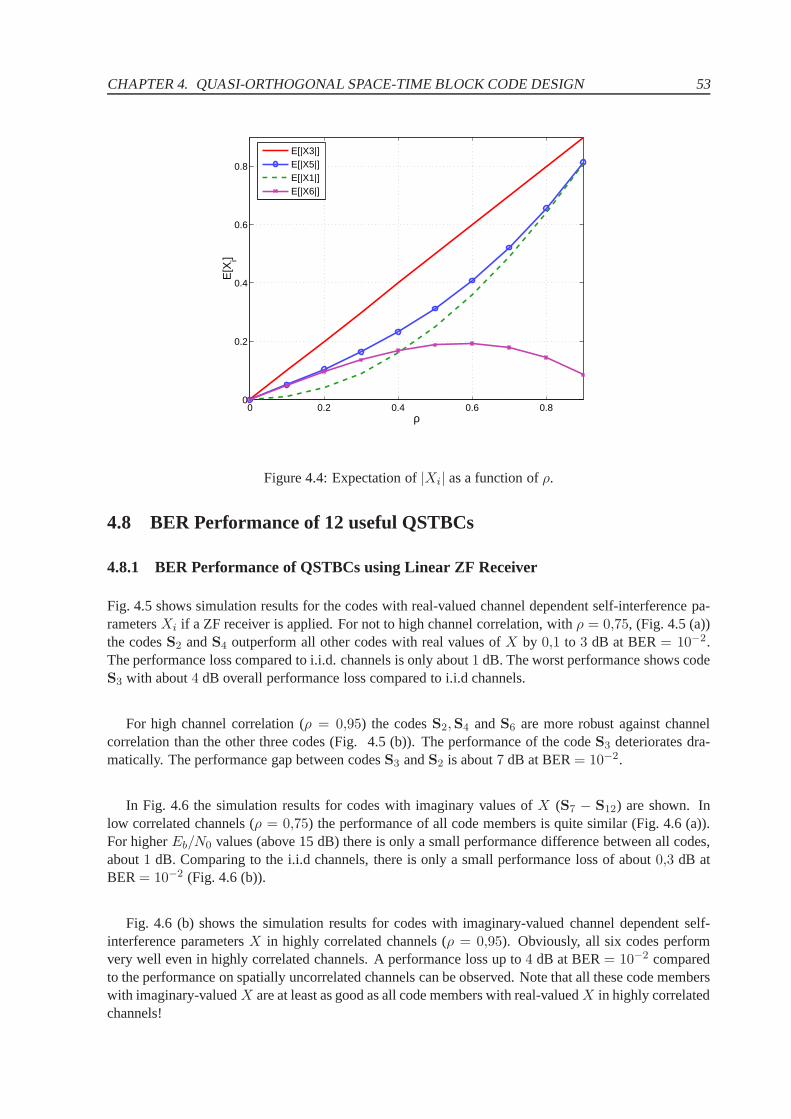
CHAPTER 4. QUASI-ORTHOGONAL SPACE-TIME BLOCK CODE DESIGN 53
0 0.2 0.4 0.6 0.80
0.2
0.4
0.6
0.8
ρ
E[X
i]
E[|X3|]E[|X5|]E[|X1|]E[|X6|]
Figure 4.4: Expectation of|Xi| as a function ofρ.
4.8 BER Performance of 12 useful QSTBCs
4.8.1 BER Performance of QSTBCs using Linear ZF Receiver
Fig. 4.5 shows simulation results for the codes with real-valued channel dependent self-interference pa-rametersXi if a ZF receiver is applied. For not to high channel correlation, withρ = 0,75, (Fig. 4.5 (a))the codesS2 andS4 outperform all other codes with real values ofX by 0,1 to 3 dB at BER= 10−2.The performance loss compared to i.i.d. channels is only about 1 dB. The worst performance shows codeS3 with about4 dB overall performance loss compared to i.i.d channels.
For high channel correlation (ρ = 0,95) the codesS2,S4 andS6 are more robust against channelcorrelation than the other three codes (Fig. 4.5 (b)). The performance of the codeS3 deteriorates dra-matically. The performance gap between codesS3 andS2 is about7 dB at BER= 10−2.
In Fig. 4.6 the simulation results for codes with imaginary values ofX (S7 − S12) are shown. Inlow correlated channels (ρ = 0,75) the performance of all code members is quite similar (Fig. 4.6 (a)).For higherEb/N0 values (above 15 dB) there is only a small performance difference between all codes,about1 dB. Comparing to the i.i.d channels, there is only a small performance loss of about0,3 dB atBER= 10−2 (Fig. 4.6 (b)).
Fig. 4.6 (b) shows the simulation results for codes with imaginary-valued channel dependent self-interference parametersX in highly correlated channels (ρ = 0,95). Obviously, all six codes performvery well even in highly correlated channels. A performanceloss up to4 dB at BER= 10−2 comparedto the performance on spatially uncorrelated channels can be observed. Note that all these code memberswith imaginary-valuedX are at least as good as all code members with real-valuedX in highly correlatedchannels!
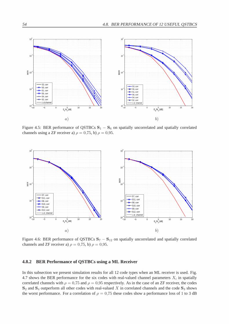
54 4.8. BER PERFORMANCE OF 12 USEFUL QSTBCS
−10 −5 0 5 10 15 2010
−4
10−3
10−2
10−1
100
Eb/N
0 [dB]
BE
R
S3, corrS5, corrS1, corrS6, corrS4, corrS2, corri.i.d.channel
−10 −5 0 5 10 15 2010
−4
10−3
10−2
10−1
100
Eb/N
0 [dB]
BE
R
S3, corrS5, corrS1, corrS6, corrS4, corrS2, corri.i.d. channel
a) b)
Figure 4.5: BER performance of QSTBCsS1 − S6 on spatially uncorrelated and spatially correlatedchannels using a ZF receiver a)ρ = 0,75, b) ρ = 0,95.
−10 −5 0 5 10 15 2010
−4
10−3
10−2
10−1
100
Eb/N
0 [dB]
BE
R
S7, corrS11, corrS8, corrS10, corrS9, corrS12, corri.i.d. channel
−10 −5 0 5 10 15 2010
−4
10−3
10−2
10−1
100
Eb/N
0 [dB]
BE
R
S7, corrS11, corrS8, corrS10, corrS9, corrS12, corri.i.d. channel
a) b)
Figure 4.6: BER performance of QSTBCsS7 − S12 on spatially uncorrelated and spatially correlatedchannels and ZF receiver a)ρ = 0,75, b) ρ = 0,95.
4.8.2 BER Performance of QSTBCs using a ML Receiver
In this subsection we present simulation results for all 12 code types when an ML receiver is used. Fig.4.7 shows the BER performance for the six codes with real-valued channel parametersXi in spatiallycorrelated channels withρ = 0,75 andρ = 0,95 respectively. As in the case of an ZF receiver, the codesS2 andS4 outperform all other codes with real-valuedX in correlated channels and the codeS3 showsthe worst performance. For a correlation ofρ = 0,75 these codes show a performance loss of1 to 3 dB
CHAPTER 4. QUASI-ORTHOGONAL SPACE-TIME BLOCK CODE DESIGN 55
at BER= 10−2 compared to the results on uncorrelated i.i.d. MIMO channels (Fig. 4.7 (a)).
−10 −5 0 5 10 1510
−4
10−3
10−2
10−1
100
Eb/N
0 [dB]
BE
R
S3, corrS5, corrS1, corrS6, corrS4, corrS2, corri.i.d. channel
−10 −5 0 5 10 1510
−4
10−3
10−2
10−1
100
Eb/N
0 [dB]
BE
R
S3, corrS5, corrS1, corrS6, corrS4, corrS2, corri.i.d. channel
a) b)
Figure 4.7: BER performance of QSTBCsS1 − S6 on spatially uncorrelated and spatially correlatedchannels and ML receiver a)ρ = 0,75, b) ρ = 0,95.
In highly correlated channels (Fig. 4.7 (b)) the performance of codeS3 degrades enormously asin the case when a ZF receiver is used. Obviously, this code collapses in highly correlated channelsregardless what receiver algorithm is applied. The BER performance for the six codes with imaginary-valued channel parametersXi in spatially correlated channels is presented in Fig. 4.8 for ρ = 0,75 (a)and forρ = 0,95 (b) respectively. For channels correlated by a factorρ = 0,75 all code members showthe same BER performance and there is an overall loss of0,5 dB compared to spatially uncorrelatedchannels. For highly correlated channels (ρ = 0,95) we can see a loss of about5 dB at BER=10−3 forall codes. In a high correlation scenario, all codes with imaginary-valuedXi perform equally; they arequite robust against channel correlation.
4.8.3 BER Performance of QSTBCs on Measured MIMO Channels
In the analysis of STBCs, mostly channel models with i.i.d. Rayleigh fading channel transfer coefficientshave been used. Since this is rather far from practical setups, it is better to use realistic MIMO channels toevaluate different transmission schemes. In [16], [57], [58] (and references therein) it was shown that therealistic MIMO channels provide a significantly lower channel capacity than the idealized i.i.d. channels.This is mainly due to spatially correlated MIMO channel coefficients. In [60] and [61] the performance ofsome codes on measured MIMO channels has been studied. In this section we investigate the behaviorof all distinct 12usefulQSTBCs defined above on measured indoor MIMO channels. Additionallywe use realistic channel parameter measurements to estimate the correlation matrices necessary for thegeneration of a Kronecker channel model as defined in Chapter2.
4.8.3.1 Measurement Setup
In order to get realistic channel parameters, model parameters are extracted form MIMO channel mea-surements, which have been performed at our Institute. In the following, some important measurement
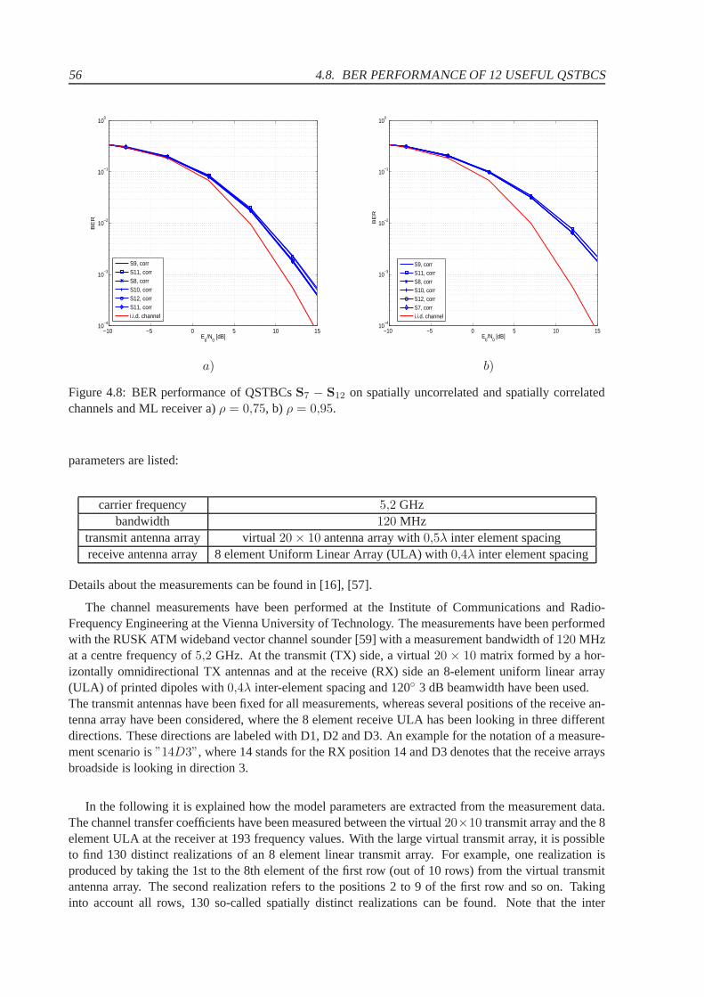
56 4.8. BER PERFORMANCE OF 12 USEFUL QSTBCS
−10 −5 0 5 10 1510
−4
10−3
10−2
10−1
100
Eb/N
0 [dB]
BE
R
S9, corrS11, corrS8, corrS10, corrS12, corrS11, corri.i.d. channel
−10 −5 0 5 10 1510
−4
10−3
10−2
10−1
100
Eb/N
0 [dB]
BE
R
S9, corrS11, corrS8, corrS10, corrS12, corrS7, corri.i.d. channel
a) b)
Figure 4.8: BER performance of QSTBCsS7 − S12 on spatially uncorrelated and spatially correlatedchannels and ML receiver a)ρ = 0,75, b) ρ = 0,95.
parameters are listed:
carrier frequency 5,2 GHzbandwidth 120 MHz
transmit antenna array virtual 20 × 10 antenna array with0,5λ inter element spacingreceive antenna array 8 element Uniform Linear Array (ULA) with0,4λ inter element spacing
Details about the measurements can be found in [16], [57].
The channel measurements have been performed at the Institute of Communications and Radio-Frequency Engineering at the Vienna University of Technology. The measurements have been performedwith the RUSK ATM wideband vector channel sounder [59] with ameasurement bandwidth of120 MHzat a centre frequency of5,2 GHz. At the transmit (TX) side, a virtual20 × 10 matrix formed by a hor-izontally omnidirectional TX antennas and at the receive (RX) side an 8-element uniform linear array(ULA) of printed dipoles with0,4λ inter-element spacing and 120◦ 3 dB beamwidth have been used.The transmit antennas have been fixed for all measurements, whereas several positions of the receive an-tenna array have been considered, where the 8 element receive ULA has been looking in three differentdirections. These directions are labeled with D1, D2 and D3.An example for the notation of a measure-ment scenario is”14D3”, where 14 stands for the RX position 14 and D3 denotes that thereceive arraysbroadside is looking in direction 3.
In the following it is explained how the model parameters areextracted from the measurement data.The channel transfer coefficients have been measured between the virtual20×10 transmit array and the 8element ULA at the receiver at 193 frequency values. With thelarge virtual transmit array, it is possibleto find 130 distinct realizations of an 8 element linear transmit array. For example, one realization isproduced by taking the 1st to the 8th element of the first row (out of 10 rows) from the virtual transmitantenna array. The second realization refers to the positions 2 to 9 of the first row and so on. Takinginto account all rows, 130 so-called spatially distinct realizations can be found. Note that the inter
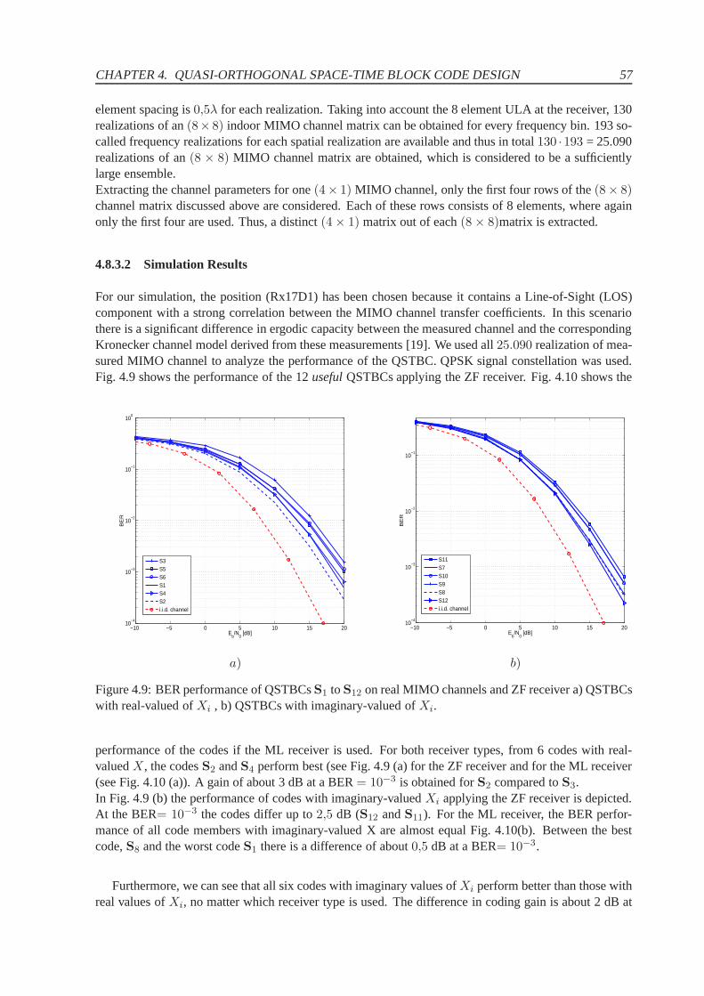
CHAPTER 4. QUASI-ORTHOGONAL SPACE-TIME BLOCK CODE DESIGN 57
element spacing is0,5λ for each realization. Taking into account the 8 element ULA at the receiver, 130realizations of an(8× 8) indoor MIMO channel matrix can be obtained for every frequency bin. 193 so-called frequency realizations for each spatial realization are available and thus in total130 ·193 = 25.090realizations of an(8 × 8) MIMO channel matrix are obtained, which is considered to be asufficientlylarge ensemble.Extracting the channel parameters for one(4× 1) MIMO channel, only the first four rows of the(8× 8)channel matrix discussed above are considered. Each of these rows consists of 8 elements, where againonly the first four are used. Thus, a distinct(4 × 1) matrix out of each(8 × 8)matrix is extracted.
4.8.3.2 Simulation Results
For our simulation, the position (Rx17D1) has been chosen because it contains a Line-of-Sight (LOS)component with a strong correlation between the MIMO channel transfer coefficients. In this scenariothere is a significant difference in ergodic capacity between the measured channel and the correspondingKronecker channel model derived from these measurements [19]. We used all25.090 realization of mea-sured MIMO channel to analyze the performance of the QSTBC. QPSK signal constellation was used.Fig. 4.9 shows the performance of the 12usefulQSTBCs applying the ZF receiver. Fig. 4.10 shows the
−10 −5 0 5 10 15 2010
−4
10−3
10−2
10−1
100
Eb/N
0 [dB]
BE
R
S3S5S6S1S4S2i.i.d. channel
−10 −5 0 5 10 15 2010
−4
10−3
10−2
10−1
Eb/N
0 [dB]
BE
R
S11S7S10S9S8S12i.i.d. channel
a) b)
Figure 4.9: BER performance of QSTBCsS1 toS12 on real MIMO channels and ZF receiver a) QSTBCswith real-valued ofXi , b) QSTBCs with imaginary-valued ofXi.
performance of the codes if the ML receiver is used. For both receiver types, from 6 codes with real-valuedX, the codesS2 andS4 perform best (see Fig. 4.9 (a) for the ZF receiver and for the ML receiver(see Fig. 4.10 (a)). A gain of about 3 dB at a BER= 10−3 is obtained forS2 compared toS3.In Fig. 4.9 (b) the performance of codes with imaginary-valuedXi applying the ZF receiver is depicted.At the BER= 10−3 the codes differ up to2,5 dB (S12 andS11). For the ML receiver, the BER perfor-mance of all code members with imaginary-valued X are almostequal Fig. 4.10(b). Between the bestcode,S8 and the worst codeS1 there is a difference of about0,5 dB at a BER= 10−3.
Furthermore, we can see that all six codes with imaginary values ofXi perform better than those withreal values ofXi, no matter which receiver type is used. The difference in coding gain is about 2 dB at
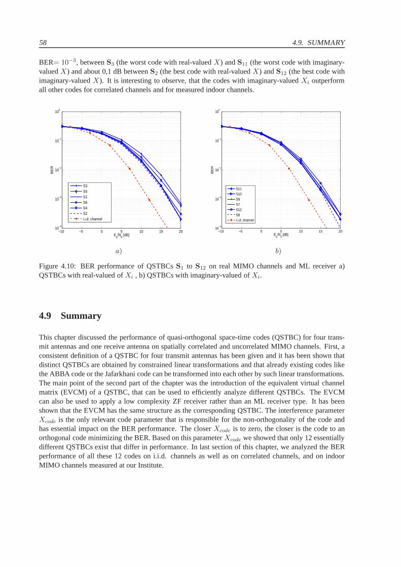
58 4.9. SUMMARY
BER= 10−3, betweenS3 (the worst code with real-valuedX) andS11 (the worst code with imaginary-valuedX) and about 0,1 dB betweenS2 (the best code with real-valuedX) andS12 (the best code withimaginary-valuedX). It is interesting to observe, that the codes with imaginary-valuedXi outperformall other codes for correlated channels and for measured indoor channels.
−10 −5 0 5 10 15 2010
−4
10−3
10−2
10−1
100
Eb/N
0 [dB]
BE
R
S3S5S1S6S4S2i.i.d. channel
−10 −5 0 5 10 15 2010
−4
10−3
10−2
10−1
100
Eb/N
0 [dB]
BE
R
S11S10S9S7S12S8i.i.d. channel
a) b)
Figure 4.10: BER performance of QSTBCsS1 to S12 on real MIMO channels and ML receiver a)QSTBCs with real-valued ofXi , b) QSTBCs with imaginary-valued ofXi.
4.9 Summary
This chapter discussed the performance of quasi-orthogonal space-time codes (QSTBC) for four trans-mit antennas and one receive antenna on spatially correlated and uncorrelated MIMO channels. First, aconsistent definition of a QSTBC for four transmit antennas has been given and it has been shown thatdistinct QSTBCs are obtained by constrained linear transformations and that already existing codes likethe ABBA code or the Jafarkhani code can be transformed into each other by such linear transformations.The main point of the second part of the chapter was the introduction of the equivalent virtual channelmatrix (EVCM) of a QSTBC, that can be used to efficiently analyze different QSTBCs. The EVCMcan also be used to apply a low complexity ZF receiver rather than an ML receiver type. It has beenshown that the EVCM has the same structure as the corresponding QSTBC. The interference parameterXcode is the only relevant code parameter that is responsible for the non-orthogonality of the code andhas essential impact on the BER performance. The closerXcode is to zero, the closer is the code to anorthogonal code minimizing the BER. Based on this parameterXcode we showed that only 12 essentiallydifferent QSTBCs exist that differ in performance. In last section of this chapter, we analyzed the BERperformance of all these 12 codes on i.i.d. channels as well as on correlated channels, and on indoorMIMO channels measured at our Institute.
Chapter 5
Quasi-Orthogonal Space-Time BlockCodes with Partial Channel Knowledge
5.1 Introduction
In previous chapters various space-time coding schemes have been presented. In the analysis of theseSTBCs it is usually assumed that the channel state information (CSI) is known perfectly at the receiverbut not at the transmitter. On the other hand, CSI can be made available at the transmitter. In some casesCSI is limited to the channel statistics whereas the actual CSI is unknown. In fact, the transmitter shouldexploit any channel information available. This knowledge, whether partial or complete, can be advan-tageously exploited to adapt the transmission strategy in order to optimize the system performance. Fullchannel knowledge at the transmitter implies that the instantaneous channel transfer matrixH is knownat the transmitter.
If the channel is known at the transmitter the channel capacity can be increased by resorting to theso-calledwater-filling principle [1]. In order to use water-filling we have to perform a singular valuedecomposition (SVD) of the MIMO channel ifH is available at the transmitter [82]. Define the SVD ofthe channel matrixH as
H = UΛVH (5.1)
whereU is annr×nr matrix,V is nt×nt complex unitary matrix andΛ is annr×nt matrix containingreal, non-negative singular valuesλ
1/2i , i = 1, 2, · · · , r andλi are at the same time the eigenvalues of
the matrixHHH (r denotes the rank of the matrixH). Applying a preprocessing of the transmit vectors and of the modified receive vectory due to
y = UHy
n = UHn
s = VHs
(5.2)
then the channel model in (2.2),y = Hs + n, can be reformulated as
y = Λs + n. (5.3)
SinceΛ is annr × nt matrix with r nonzero diagonal elements, we have effectivelyr parallel and inde-pendent transmission channels. When we transmit a vectors through a MIMO channel in this way, we
59
60 5.1. INTRODUCTION
excite the so-called eigenmodes of the channel. Each eigenmode is directly related to one of the channeleigen vectors and each mode is received with a gain proportional to the corresponding singular value, orin a quadratic sense, with a power gain equal toλi. Thus the eigenvalues ofHHH play a fundamentalrole in characterizing the performance of a MIMO channel.
With full CSI at the transmitter, the water-filling transmission scheme pours power on the eigenmodesof the MIMO channel in such a way that more power is delivered to stronger eigenmodes and less or nopower to the weaker eigenmodes. This algorithm is an optimalpower allocation algorithm. Since thisalgorithm only concentrates on good-quality channels and rejects the bad ones during each channel real-ization, it is easy to understand that this method yields a capacity that is equal or better than the situationwhen the channel is unknown to the transmitter.Another strategy with full channel knowledge at the transmitter is beamforming[62], [63] where onlythe strongest eigenmode is used. However, beamforming is a specific example of signal processing at thetransmitter, as it works only in the spatial domain. Note however, that this technique requires transmitamplifiers which are highly linear [62]. At low SNR beamforming is a spectrally efficient transmissionscheme and at high SNR, where more channel eigenmodes can be used, water-filling is better for achiev-ing high channel capacity.
In general and assuming an ideal channel knowledge at the transmitter, a transmission using a STBCperforms worse than a system using a beamforming technique [69], [70]. This stems from the fact, thatSTBC systems spreads the available power uniformly in all directions in space, while beamforming usesinformation about the channel to steer energy in the direction of the receiver. The gap in the performancebetween the two methods can be quite significant, especiallyin highly correlated channels.One general drawback of methods relying on complete CSI at the transmitter is feasibility and the needfor a feedback path delivering CSI from the receiver to the transmitter. In practical situations, the feed-back channel may allow only partial CSI to be returned to the transmitter in order to save bandwidth inthe feedback path. Partial channel knowledge might refer tosome parameters of the instantaneous chan-nel or some statistics on the channel. To close the gap between the beamforming system and the STBCbased system, improved space time coding using feedback of partial or full channel state information tothe transmitter may be used.
5.1.1 QSTBCs Exploiting Partial CSI using Limited Feedback
Designing STBCs and evaluating the performance of STBCs in transmission schemes with feedback hasbeen an intensive area of research resulting in several different transmit strategies [64] - [81]. PartialCSI feedback can correspond to a quantized channel estimate[68], or can be used to find an optimumindex in a finite set of precoder matrices [69],[71], or can beused for antenna selection [77]-[81] or forcode selection [64]-[67]. Each of these partial feedback options returns a limited number of channelinformation bits from the receiver to the transmitter. Due to practical limitations, the number of feedbackbits per code block returned from the receiver to the transmitter should be kept as small as possible.
Diversity order is an important indicator of the performance of any multi-antenna transmission scheme.Since QSTBCs without feedback do not achieve full diversity, research on QSTBCs with partial feed-back is beginning to gain more and more attention. For instance, a very simple and clever scheme waspresented in [64] where block codes with feedback have been used. On the transmitter side code se-lection according to the feedback bit is performed. Selecting one of two possible code matrices alreadyleads to full diversity and some coding gain. However, this scheme requires also perfect synchronizationof transmitter and receiver. If this synchronization is erroneous or the feedback information is decoded
CHAPTER 5. PERFORMANCE OF QSTBCS WITH PARTIAL CHANNEL KNOWLEDGE 61
incorrectly this concept easily looses most of its benefits.One more disadvantage of the scheme pro-posed in [64] is that by increasing the number of transmit antennas, the required number of feedback bitsincreases proportional.In [65], [67] we presented recently an even simpler version of a channel adaptive code selection(CACS)in combination with QSTBCs. The receiver returns one or two feedback bits per fading block and (de-pending on the number of returned bits) the transmitter switches between two or four predefined QSTBCsto minimize the channel dependent interference parameterX. In this way full diversity and nearly full-orthogonality can be achieved with an ML receiver as well as with a simple ZF receiver. This methodcan be applied to any number of transmit antennas without increasing the required number of feedbackbits. In [61, 66], our simulations have been applied on correlated MIMO channels and measured MIMOindoor channels, and there we have shown that QSTBCs with oursimple feedback scheme are robustagainst channel variations, and that they perform very welleven on highly correlated channels. Thismethod will be explained in detail in the next section.
In order to reduce the implementation complexity of MIMO systems (e.g. the high number of radio-frequency (RF) chains on both link ends)channel adaptive antenna selection(CAAS) at the transmitterand/or at the receiver side has been proposed in [77]-[81], where only a subset of ”best” antennas is usedfor transmitting the data. CAAS was first combined using OSTBCs in [77, 78]. In [77], the transmitselection criterion was based on maximization of the Frobenius norm of the channel transfer matrix. Ithas been shown that this scheme achieves full diversity, as if all the transmit antennas were used.In [80, 81] transmit and receive CAAS with QSTBC for four transmit antennas and a ZF receiver hasbeen proposed. The selection criterion is based on the analytic expression for the BER given in Chapter4, Eqn. (4.46) and maximizes the termh2(1 − X2) [81]. This CAAS will be described in detail in thenext section.
5.2 Channel Adaptive Code Selection (CACS)
In this section a simple and effective way to adapt a full rateQSTBCs over2n transmit antennas tothe actual channel is proposed achieving full diversity, nearly full orthogonality and at the same time alow bit error rate. A feedback system returning one or two bits per code block from the receiver to thetransmitter is applied. Depending on the feed-back information the transmitter switches between two orfour predefined QSTBCs which only differ in the resulting channel dependent interference parameter.The transmitter chooses that code that minimizes the channel depended interference parameterX whichis responsible for the diversity loss of the QSTBC. With thissimple scheme, a ZF as well as an MLreceiver achieves nearly optimum system performance.
5.2.1 CACS with One Feedback Bit per Code Block
The feedback scheme using one bit feedback per code block sent from the receiver to the transmittercharacterizing the channel will be explained first. The transmission scheme is depicted in Fig. 5.1. Fourtransmit antennas and one receive antenna and an actual channel transfer vectorh = [h1, h2, h3, h4]
T
are considered. The channel transfer elementshi may fade in any arbitrary way but it is assumed thatthey are constant during the code block of length four. The signal transmission is described (as explainedin the Chapter 4, Eqn. (4.28)) by
r = Sh + n, (5.4)
wherer is the (4 × 1) vector of received signals of one the code-block within foursuccessive timeslots. S is the predefined QSTBC, eitherS1, as defined in (5.5), orS2 defined in (5.6) depending on
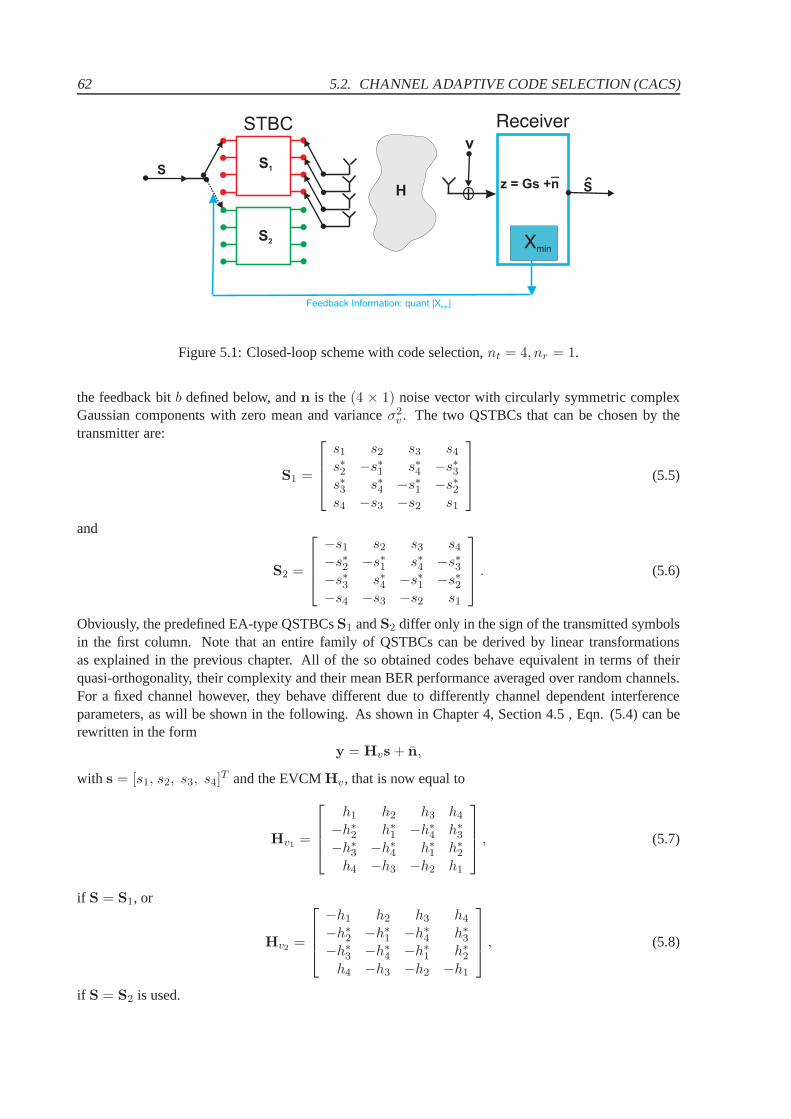
62 5.2. CHANNEL ADAPTIVE CODE SELECTION (CACS)
H
Feedback Information: quant |X |min
S1
S2
STBC
z = Gs +n
Receiver
Xmin
S
v
S
Figure 5.1: Closed-loop scheme with code selection,nt = 4, nr = 1.
the feedback bitb defined below, andn is the(4 × 1) noise vector with circularly symmetric complexGaussian components with zero mean and varianceσ2
v . The two QSTBCs that can be chosen by thetransmitter are:
S1 =
s1 s2 s3 s4
s∗2 −s∗1 s∗4 −s∗3s∗3 s∗4 −s∗1 −s∗2s4 −s3 −s2 s1
(5.5)
and
S2 =
−s1 s2 s3 s4
−s∗2 −s∗1 s∗4 −s∗3−s∗3 s∗4 −s∗1 −s∗2−s4 −s3 −s2 s1
. (5.6)
Obviously, the predefined EA-type QSTBCsS1 andS2 differ only in the sign of the transmitted symbolsin the first column. Note that an entire family of QSTBCs can bederived by linear transformationsas explained in the previous chapter. All of the so obtained codes behave equivalent in terms of theirquasi-orthogonality, their complexity and their mean BER performance averaged over random channels.For a fixed channel however, they behave different due to differently channel dependent interferenceparameters, as will be shown in the following. As shown in Chapter 4, Section 4.5 , Eqn. (5.4) can berewritten in the form
y = Hvs + n,
with s = [s1, s2, s3, s4]T and the EVCMHv, that is now equal to
Hv1=
h1 h2 h3 h4
−h∗2 h∗
1 −h∗4 h∗
3
−h∗3 −h∗
4 h∗1 h∗
2
h4 −h3 −h2 h1
, (5.7)
if S = S1, or
Hv2=
−h1 h2 h3 h4
−h∗2 −h∗
1 −h∗4 h∗
3
−h∗3 −h∗
4 −h∗1 h∗
2
h4 −h3 −h2 −h1
, (5.8)
if S = S2 is used.
CHAPTER 5. PERFORMANCE OF QSTBCS WITH PARTIAL CHANNEL KNOWLEDGE 63
In both cases we obtain non-orthogonal Grammian matrices with the same structure
Gi = HHviHvi = HviH
Hvi
= h2
1 0 0 Xi
0 1 −Xi 00 −Xi 1 0
X1 0 0 1
(5.9)
for i = 1,2, with
h2 = |h1|2 + |h2|2 + |h3|2 + |h4|2,
but different values ofXi, namely
X1 =2Re(h1h
∗4 − h2h
∗3)
h2, (5.10)
if S1 is sent, and
X2 =2Re(−h1h
∗4 − h2h
∗3)
h2, (5.11)
if S2 is sent.
It is well known thatG should approximate a scaled identity-matrix as far as possible to achieve fulldiversity and optimum BER performance [47]. IfG is a scaled identity matrix, we have an orthogonalSTBC and we could use a simple linear matrix multiplication of y by HH
v (corresponding to a simplematched filter operation) at the receiver to decouple the channel perfectly and to obtain full diversityorderd = 4. Otherwise,Xi leads to a partial interference betweenh1 andh4 and betweenh2 andh3.This means,X should be as small as possible. AsGi indicates, our scheme inherently supports fulldiversityd = 4, if Xi can be made zero.
Thus, our code selection strategy is to transmit that codeS1 or S2 that minimizes|X|. S2 is obtainedfrom S1 by a linear transformation, explained in Chapter 4, Eqn. (4.20):
S2 = S1 · I1, (5.12)
whereI1 is a diagonal(4 × 4) matrix that changes the sign of the 1st column of the matrixS1. Bychanging the sign of the first column of the QSTBCS1 we change the sign of the first term of the channeldependent self-interference parameterX given in (5.10) and (5.11). As it is assumed that the receiverhasfull information of the channel, knowingh1 to h4, the receiver can computeX1 andX2 due to (5.10) and(5.11). With this information the receiver returns the feedback bitb informing the transmitter to selectthat code blockSi(i = 1, 2) which leads to the smaller value ofXi. With this information the transmitterswitches between the predefined QSTBCS1 andS2 such that the resulting|X| will be min(|X1|, |X2|).Obviously the control information sent back to the transmitter only needs one feedback bit per codeblock. In our simulations it is assumed that the channel varies slowly such that the delay of the feedbackinformation can be neglected. In this way we obtain very small values ofX, due to the fact that in (5.10),(5.11) two approximately equally valued terms are subtracted and thus at least partially compensate eachother. Nevertheless, some performance loss due to the non vanishing value ofX is expected resultingfrom the residual interference between the signal elementss1 ands4, ands2 ands3, respectively.
64 5.2. CHANNEL ADAPTIVE CODE SELECTION (CACS)
5.2.2 Probability Distribution of the Resulting Interference Parameter W
As explained before, the main idea of our adaptive space-time coding is to reduce the resulting interfer-ence parameterX in order to improve the ”quasi-orthogonality” of the virtual equivalent channel matrix.Therefore, we want to derive the corresponding probabilitydensity of this resulting random interferencevariableX in case of switching between the two predefined QSTBCs,S1 andS2.If the channel coefficientshi are i.i.d. random complex Gaussian distributed variables,then the proba-bility density function ofX is given as (see Chapter 4, Section 4.7.5, Eqn. (4.69) )
fX(x) =
{
34(1 − x2) ; |x| < 1,0 ; else .
To derive the probability density function of min(|X1|, |X2|) in case of one feedback bit per code block,the pdfs of two random variables need to be considered. For this purpose a new random variable (RV) isdefined as:
W =
{
X1 ; if |X1| < |X2|X2 ; else .
(5.13)
Due to its symmetry only the one sided (positive) pdf is considered and following [39][p. 195] we obtain:
fW (w) = fX1(w) + fX2
(w) − fX1(w)FX2
(w)
− FX1(w)fX2
(w)
= 2fX1(w)(1 − FX1
(w)) (5.14)
whereX1,X2 are assumed to be two statistically independent random variables. With (4.69), the finalsolution forfW (w) is :
fW (w) =
{
32(1 − w2)
[
1 − 32 |w|(1 − w2
3 )]
; |w| ≤ 1
0 ; else .(5.15)
Simulations results verifying this result are presented inFig. 5.2 further ahead.
5.2.3 CACS with Two Control Bits fed back from the Receiver tothe Transmitter
In a similar way as discussed in Section 5.2.1, we can switch between four different QSTBCs at thetransmitter to improve our system further. Let us discuss the case when we are allowed to send two bitsb1, b2 as a feedback information from the receiver to the transmitter. Now, we let the transmitter switchbetween four very similar QSTBCs, namelyS1 andS2 defined in (5.5) and (5.6) and two new codematricesS3,S4 defined as:
S3 =
js1 −js2 s3 s4
js∗2 js∗1 s∗4 −s∗3js∗3 −js∗4 −s∗1 −s∗2js4 js3 −s2 s1
(5.16)
and
S4 =
js1 js2 s3 s4
js∗2 −js∗1 s∗4 −s∗3js∗3 js∗4 −s∗1 −s∗2js4 −js3 −s2 s1
. (5.17)
The corresponding EVCM,Hv, is equal to:
Hv3=
jh1 −jh2 h3 h4
−jh∗2 −jh∗
1 −h∗4 h∗
3
−h∗3 −h∗
4 −jh∗1 jh∗
2
h4 −h3 jh2 jh1
(5.18)
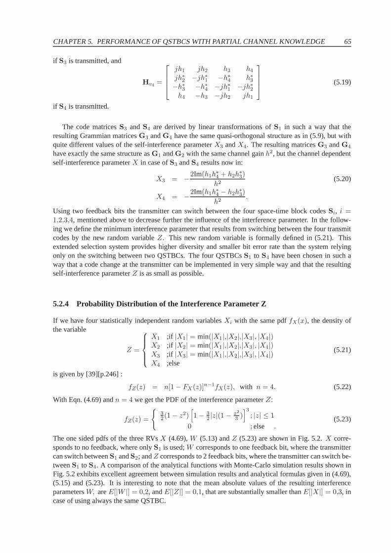
CHAPTER 5. PERFORMANCE OF QSTBCS WITH PARTIAL CHANNEL KNOWLEDGE 65
if S3 is transmitted, and
Hv4=
jh1 jh2 h3 h4
jh∗2 −jh∗
1 −h∗4 h∗
3
−h∗3 −h∗
4 −jh∗1 −jh∗
2
h4 −h3 −jh2 jh1
(5.19)
if S4 is transmitted.
The code matricesS3 andS4 are derived by linear transformations ofS1 in such a way that theresulting Grammian matricesG3 andG4 have the same quasi-orthogonal structure as in (5.9), but withquite different values of the self-interference parameterX3 andX4. The resulting matricesG3 andG4
have exactly the same structure asG1 andG2 with the same channel gainh2, but the channel dependentself-interference parameterX in case ofS3 andS4 results now in:
X3 = −2Im(h1h∗4 + h2h
∗3)
h2(5.20)
X4 = −2Im(h1h∗4 − h2h
∗3)
h2.
Using two feedback bits the transmitter can switch between the four space-time block codesSi, i =1,2,3,4, mentioned above to decrease further the influence of the interference parameter. In the follow-ing we define the minimum interference parameter that results from switching between the four transmitcodes by the new random variableZ. This new random variable is formally defined in (5.21). Thisextended selection system provides higher diversity and smaller bit error rate than the system relyingonly on the switching between two QSTBCs. The four QSTBCsS1 to S4 have been chosen in such away that a code change at the transmitter can be implemented in very simple way and that the resultingself-interference parameterZ is as small as possible.
5.2.4 Probability Distribution of the Interference Parameter Z
If we have four statistically independent random variablesXi with the same pdffX(x), the density ofthe variable
Z =
X1 ;if |X1| = min(|X1|,|X2|,|X3|, |X4|)X2 ;if |X2| = min(|X1|,|X2|,|X3|, |X4|)X3 ;if |X3| = min(|X1|,|X2|,|X3|, |X4|)X4 ;else
(5.21)
is given by [39][p.246] :
fZ(z) = n[1 − FX(z)]n−1fX(z), with n = 4. (5.22)
With Eqn. (4.69) andn = 4 we get the PDF of the interference parameterZ:
fZ(z) =
{
32(1 − z2)
[
1 − 32 |z|(1 − z2
3 )]3
; |z| ≤ 1
0 ; else .(5.23)
The one sided pdfs of the three RVsX (4.69),W (5.13) andZ (5.23) are shown in Fig. 5.2.X corre-sponds to no feedback, where onlyS1 is used;W corresponds to one feedback bit, where the transmittercan switch betweenS1 andS2; andZ corresponds to 2 feedback bits, where the transmitter can switch be-tweenS1 to S4. A comparison of the analytical functions with Monte-Carlosimulation results shown inFig. 5.2 exhibits excellent agreement between simulation results and analytical formulas given in (4.69),(5.15) and (5.23). It is interesting to note that the mean absolute values of the resulting interferenceparametersW, areE[|W |] = 0,2, andE[|Z|] = 0,1, that are substantially smaller thanE[|X|] = 0,3, incase of using always the same QSTBC.
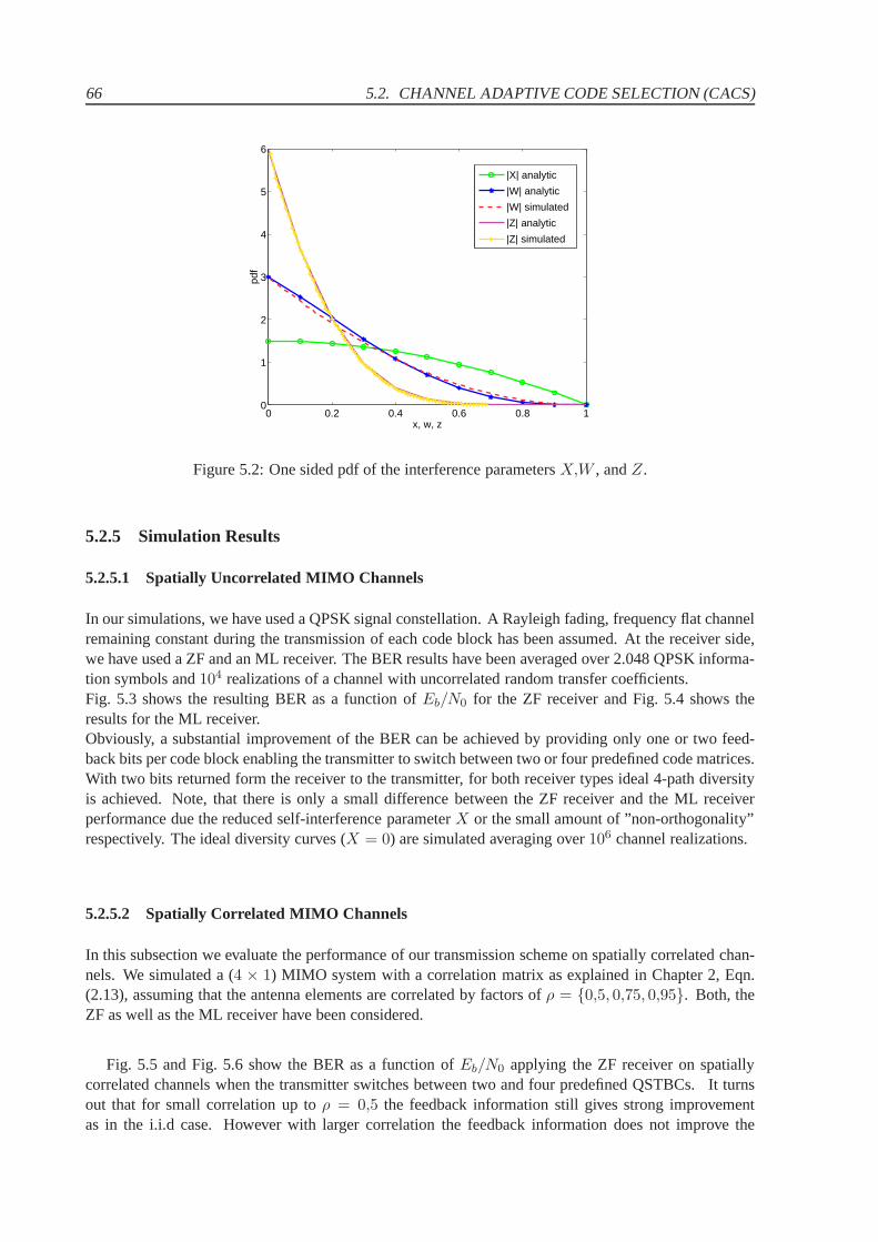
66 5.2. CHANNEL ADAPTIVE CODE SELECTION (CACS)
0 0.2 0.4 0.6 0.8 10
1
2
3
4
5
6
x, w, z
|X| analytic
|W| analytic
|W| simulated
|Z| analytic
|Z| simulated
Figure 5.2: One sided pdf of the interference parametersX,W , andZ.
5.2.5 Simulation Results
5.2.5.1 Spatially Uncorrelated MIMO Channels
In our simulations, we have used a QPSK signal constellation. A Rayleigh fading, frequency flat channelremaining constant during the transmission of each code block has been assumed. At the receiver side,we have used a ZF and an ML receiver. The BER results have been averaged over 2.048 QPSK informa-tion symbols and104 realizations of a channel with uncorrelated random transfer coefficients.Fig. 5.3 shows the resulting BER as a function ofEb/N0 for the ZF receiver and Fig. 5.4 shows theresults for the ML receiver.Obviously, a substantial improvement of the BER can be achieved by providing only one or two feed-back bits per code block enabling the transmitter to switch between two or four predefined code matrices.With two bits returned form the receiver to the transmitter,for both receiver types ideal 4-path diversityis achieved. Note, that there is only a small difference between the ZF receiver and the ML receiverperformance due the reduced self-interference parameterX or the small amount of ”non-orthogonality”respectively. The ideal diversity curves (X = 0) are simulated averaging over106 channel realizations.
5.2.5.2 Spatially Correlated MIMO Channels
In this subsection we evaluate the performance of our transmission scheme on spatially correlated chan-nels. We simulated a (4 × 1) MIMO system with a correlation matrix as explained in Chapter 2, Eqn.(2.13), assuming that the antenna elements are correlated by factors ofρ = {0,5, 0,75, 0,95}. Both, theZF as well as the ML receiver have been considered.
Fig. 5.5 and Fig. 5.6 show the BER as a function ofEb/N0 applying the ZF receiver on spatiallycorrelated channels when the transmitter switches betweentwo and four predefined QSTBCs. It turnsout that for small correlation up toρ = 0,5 the feedback information still gives strong improvementas in the i.i.d case. However with larger correlation the feedback information does not improve the
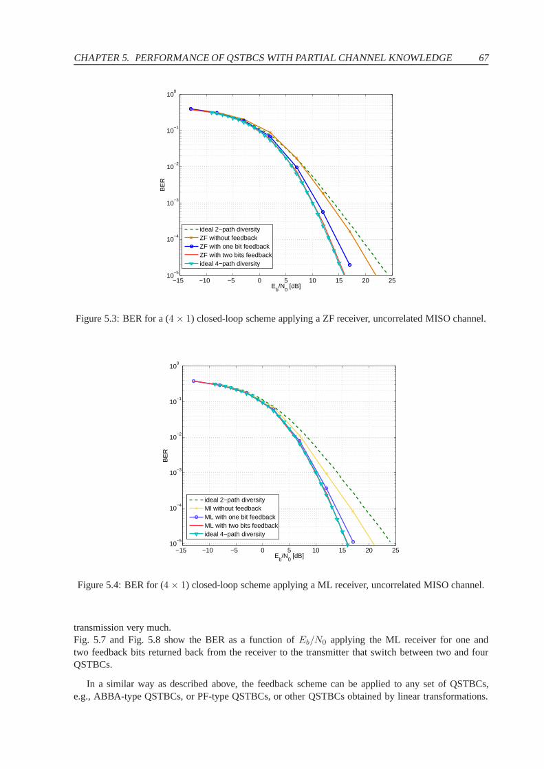
CHAPTER 5. PERFORMANCE OF QSTBCS WITH PARTIAL CHANNEL KNOWLEDGE 67
−15 −10 −5 0 5 10 15 20 2510
−5
10−4
10−3
10−2
10−1
100
Eb/N
0 [dB]
BE
R
ideal 2−path diversityZF without feedbackZF with one bit feedbackZF with two bits feedbackideal 4−path diversity
Figure 5.3: BER for a (4 × 1) closed-loop scheme applying a ZF receiver, uncorrelated MISO channel.
−15 −10 −5 0 5 10 15 20 2510
−5
10−4
10−3
10−2
10−1
100
Eb/N
0 [dB]
BE
R
ideal 2−path diversityMl without feedbackML with one bit feedbackML with two bits feedbackideal 4−path diversity
Figure 5.4: BER for (4 × 1) closed-loop scheme applying a ML receiver, uncorrelated MISO channel.
transmission very much.Fig. 5.7 and Fig. 5.8 show the BER as a function ofEb/N0 applying the ML receiver for one andtwo feedback bits returned back from the receiver to the transmitter that switch between two and fourQSTBCs.
In a similar way as described above, the feedback scheme can be applied to any set of QSTBCs,e.g., ABBA-type QSTBCs, or PF-type QSTBCs, or other QSTBCs obtained by linear transformations.
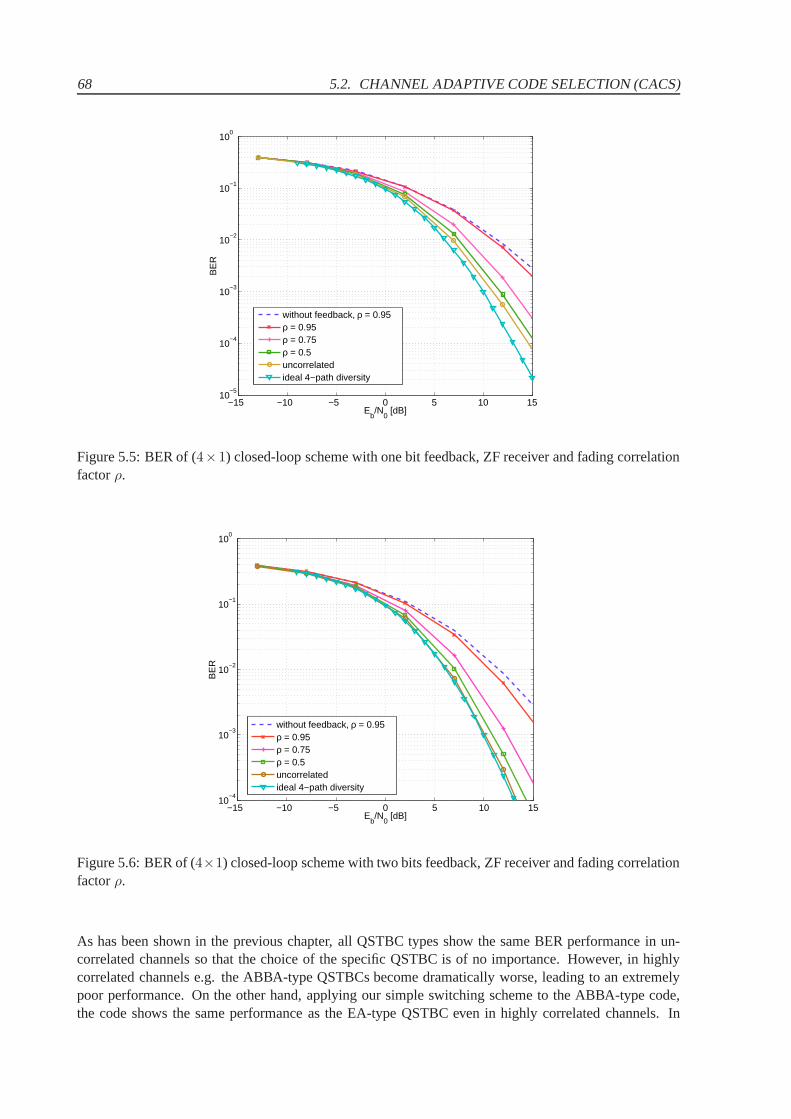
68 5.2. CHANNEL ADAPTIVE CODE SELECTION (CACS)
−15 −10 −5 0 5 10 1510
−5
10−4
10−3
10−2
10−1
100
Eb/N
0 [dB]
BE
R
without feedback, ρ = 0.95ρ = 0.95ρ = 0.75ρ = 0.5uncorrelatedideal 4−path diversity
Figure 5.5: BER of (4×1) closed-loop scheme with one bit feedback, ZF receiver and fading correlationfactorρ.
−15 −10 −5 0 5 10 1510
−4
10−3
10−2
10−1
100
Eb/N
0 [dB]
BE
R
without feedback, ρ = 0.95ρ = 0.95ρ = 0.75ρ = 0.5uncorrelatedideal 4−path diversity
Figure 5.6: BER of (4×1) closed-loop scheme with two bits feedback, ZF receiver andfading correlationfactorρ.
As has been shown in the previous chapter, all QSTBC types show the same BER performance in un-correlated channels so that the choice of the specific QSTBC is of no importance. However, in highlycorrelated channels e.g. the ABBA-type QSTBCs become dramatically worse, leading to an extremelypoor performance. On the other hand, applying our simple switching scheme to the ABBA-type code,the code shows the same performance as the EA-type QSTBC evenin highly correlated channels. In
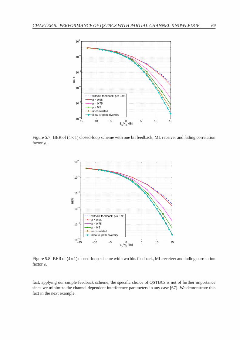
CHAPTER 5. PERFORMANCE OF QSTBCS WITH PARTIAL CHANNEL KNOWLEDGE 69
−15 −10 −5 0 5 10 1510
−5
10−4
10−3
10−2
10−1
100
Eb/N
0 [dB]
BE
R
without feedback, ρ = 0.95ρ = 0.95ρ = 0.75ρ = 0.5uncorrelatedideal 4−path diversity
Figure 5.7: BER of (4×1) closed-loop scheme with one bit feedback, ML receiver and fading correlationfactorρ.
−15 −10 −5 0 5 10 1510
−5
10−4
10−3
10−2
10−1
100
Eb/N
0 [dB]
BE
R
without feedback, ρ = 0.95ρ = 0.95ρ = 0.75ρ = 0.5uncorrelatedideal 4−path diversity
Figure 5.8: BER of (4×1) closed-loop scheme with two bits feedback, ML receiver andfading correlationfactorρ.
fact, applying our simple feedback scheme, the specific choice of QSTBCs is not of further importancesince we minimize the channel dependent interference parameters in any case [67]. We demonstrate thisfact in the next example.
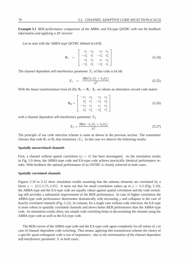
70 5.2. CHANNEL ADAPTIVE CODE SELECTION (CACS)
Example 5.1 BER performance comparison of the ABBA- and EA-type QSTBC with one bit feedbackinformation and applying a ZF receiver
Let us start with the ABBA-type QSTBC defined in (4.8):
S1 =
s1 s2 s3 s4
−s∗2 s∗1 −s∗4 s∗3s3 s4 s1 s2
−s∗4 s∗3 −s∗2 s∗1
. (5.24)
The channel dependent self-interference parameterX1 of this code is (4.54)
X1 =2Re(h1h
∗3 + h2h
∗4)
h2. (5.25)
With the linear transformation from (4.20),S2 = S1 · I1, we obtain an alternative second code matrix
S2 =
−s1 s2 s3 s4
s∗2 s∗1 −s∗4 s∗3−s3 s4 s1 s2
s∗4 s∗3 −s∗2 s∗1
(5.26)
with a channel dependent self-interference parameterX2
X2 =2Re(−h1h
∗3 + h2h
∗4)
h2. (5.27)
The principle of our code selection scheme is same as shown inthe previous section: The transmitterchooses that codeS1 or S2 that minimizes|Xi|. In this case we observe the following results:
Spatially uncorrelated channels
First, a channel without spatial correlation (ρ = 0) has been investigated. As the simulation resultsin Fig. 5.9 show, the ABBA-type code and EA-type code achievepractically identical performance re-sults. With feedback the optimal performance of an OSTBC is closely achieved in both cases.
Spatially correlated channels
Figures 5.10 to 5.12 show simulation results assuming that the antenna elements are correlated by afactor ρ = {0,5, 0,75, 0,95}. It turns out that for small correlation values up toρ = 0,5 (Fig. 5.10),the ABBA-type and the EA-type code are equally robust against spatial correlation and the code switch-ing still provides a substantial improvement of the BER performance. In case of higher correlation theABBA-type code performance deteriorates dramatically with increasingρ and collapses in the case ofheavily correlated channels (Fig. 5.12). In contrast, for asingle case without code selection, the EA-typeis more robust in spatially correlated channels and shows better BER performance than the ABBA-typecode. As simulation results show, our simple code switchinghelps in decorrelating the channel using theABBA-type code as well as the EA-type code.
The BER-curves of the ABBA-type code and the EA-type code agree completely for all values ofρ incase of channel dependent code switching. That means, applying this transmission scheme the choice ofa specific quasi-orthogonal code is not of importance -due to the minimization of the channel dependentself-interference parameterX in both cases.
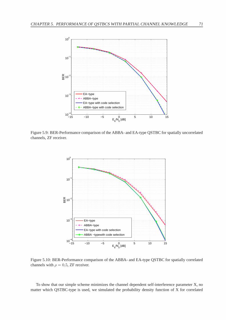
CHAPTER 5. PERFORMANCE OF QSTBCS WITH PARTIAL CHANNEL KNOWLEDGE 71
−15 −10 −5 0 5 10 1510
−4
10−3
10−2
10−1
100
Eb/N
0 [dB]
BE
R
EA−type
ABBA−type
EA−type with code selection
ABBA−type with code selection
Figure 5.9: BER-Performance comparison of the ABBA- and EA-type QSTBC for spatially uncorrelatedchannels, ZF receiver.
−15 −10 −5 0 5 10 1510
−4
10−3
10−2
10−1
100
Eb/N
0 [dB]
BE
R
EA−type
ABBA−type
EA−type with code selection
ABBA −typewith code selection
Figure 5.10: BER-Performance comparison of the ABBA- and EA-type QSTBC for spatially correlatedchannels withρ = 0,5, ZF receiver.
To show that our simple scheme minimizes the channel dependent self-interference parameter X, nomatter which QSTBC-type is used, we simulated the probability density function of X for correlated
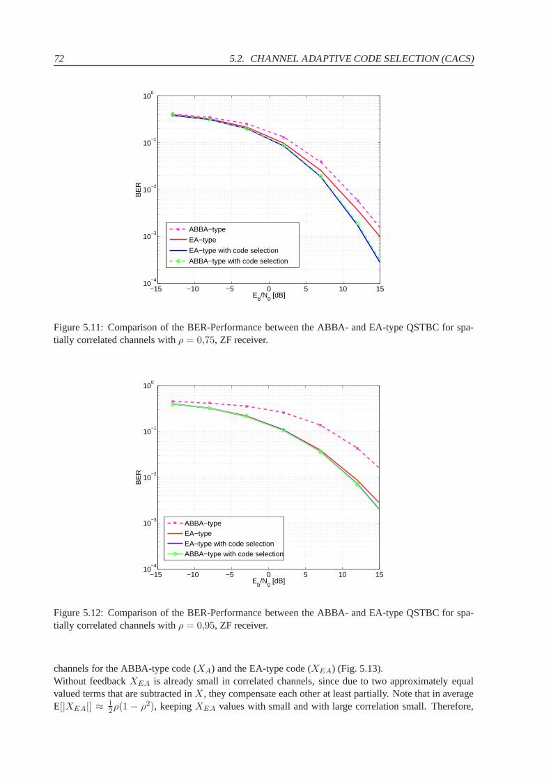
72 5.2. CHANNEL ADAPTIVE CODE SELECTION (CACS)
−15 −10 −5 0 5 10 1510
−4
10−3
10−2
10−1
100
Eb/N
0 [dB]
BE
R
ABBA−type
EA−type
EA−type with code selection
ABBA−type with code selection
Figure 5.11: Comparison of the BER-Performance between theABBA- and EA-type QSTBC for spa-tially correlated channels withρ = 0,75, ZF receiver.
−15 −10 −5 0 5 10 1510
−4
10−3
10−2
10−1
100
Eb/N
0 [dB]
BE
R
ABBA−typeEA−typeEA−type with code selectionABBA−type with code selection
Figure 5.12: Comparison of the BER-Performance between theABBA- and EA-type QSTBC for spa-tially correlated channels withρ = 0,95, ZF receiver.
channels for the ABBA-type code (XA) and the EA-type code (XEA) (Fig. 5.13).Without feedbackXEA is already small in correlated channels, since due to two approximately equalvalued terms that are subtracted inX, they compensate each other at least partially. Note that inaverageE[|XEA|] ≈ 1
2ρ(1 − ρ2), keepingXEA values with small and with large correlation small. Therefore,
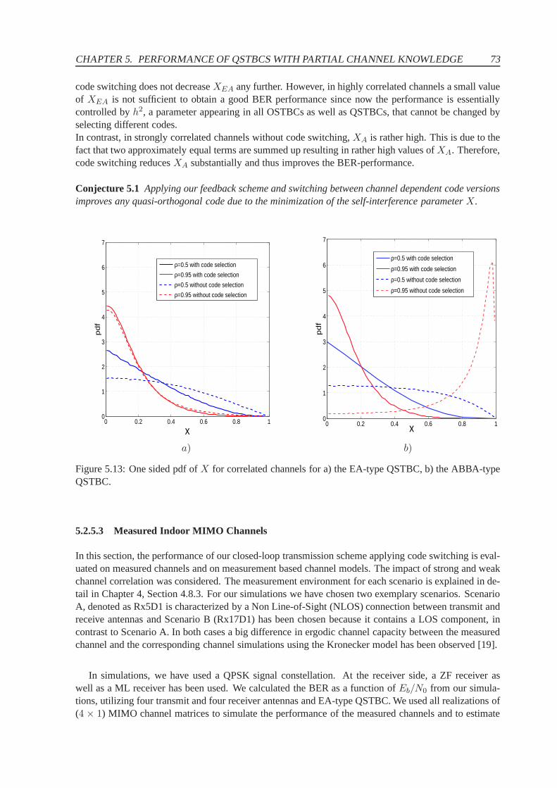
CHAPTER 5. PERFORMANCE OF QSTBCS WITH PARTIAL CHANNEL KNOWLEDGE 73
code switching does not decreaseXEA any further. However, in highly correlated channels a smallvalueof XEA is not sufficient to obtain a good BER performance since now the performance is essentiallycontrolled byh2, a parameter appearing in all OSTBCs as well as QSTBCs, that cannot be changed byselecting different codes.In contrast, in strongly correlated channels without code switching,XA is rather high. This is due to thefact that two approximately equal terms are summed up resulting in rather high values ofXA. Therefore,code switching reducesXA substantially and thus improves the BER-performance.
Conjecture 5.1 Applying our feedback scheme and switching between channeldependent code versionsimproves any quasi-orthogonal code due to the minimizationof the self-interference parameterX.
0 0.2 0.4 0.6 0.8 10
1
2
3
4
5
6
7
x
pd
f
ρ=0.5 with code selection
ρ=0.95 with code selection
ρ=0.5 without code selection
ρ=0.95 without code selection
0 0.2 0.4 0.6 0.8 10
1
2
3
4
5
6
7
x
pd
f
ρ=0.5 with code selection
ρ=0.95 with code selection
ρ=0.5 without code selection
ρ=0.95 without code selection
a) b)
Figure 5.13: One sided pdf ofX for correlated channels for a) the EA-type QSTBC, b) the ABBA-typeQSTBC.
5.2.5.3 Measured Indoor MIMO Channels
In this section, the performance of our closed-loop transmission scheme applying code switching is eval-uated on measured channels and on measurement based channelmodels. The impact of strong and weakchannel correlation was considered. The measurement environment for each scenario is explained in de-tail in Chapter 4, Section 4.8.3. For our simulations we havechosen two exemplary scenarios. ScenarioA, denoted as Rx5D1 is characterized by a Non Line-of-Sight (NLOS) connection between transmit andreceive antennas and Scenario B (Rx17D1) has been chosen because it contains a LOS component, incontrast to Scenario A. In both cases a big difference in ergodic channel capacity between the measuredchannel and the corresponding channel simulations using the Kronecker model has been observed [19].
In simulations, we have used a QPSK signal constellation. Atthe receiver side, a ZF receiver aswell as a ML receiver has been used. We calculated the BER as a function ofEb/N0 from our simula-tions, utilizing four transmit and four receiver antennas and EA-type QSTBC. We used all realizations of(4 × 1) MIMO channel matrices to simulate the performance of the measured channels and to estimate
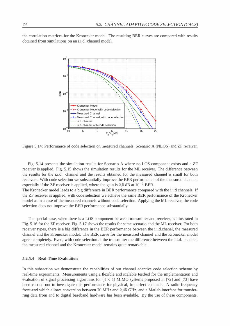
74 5.2. CHANNEL ADAPTIVE CODE SELECTION (CACS)
the correlation matrices for the Kronecker model. The resulting BER curves are compared with resultsobtained from simulations on an i.i.d. channel model.
−10 −5 0 5 10 15 2010
−4
10−3
10−2
10−1
100
Eb/N
0 [dB]
BE
R
Kronecker ModelKronecker Model with code selectionMeasured ChannelMeasured Channel with code selectioni.i.d. channeli.i.d. channel with code selection
Figure 5.14: Performance of code selection on measured channels, Scenario A (NLOS) and ZF receiver.
Fig. 5.14 presents the simulation results for Scenario A where no LOS component exists and a ZFreceiver is applied. Fig. 5.15 shows the simulation resultsfor the ML receiver. The difference betweenthe results for the i.i.d. channel and the results obtained for the measured channel is small for bothreceivers. With code selection we substantially improve the BER performance of the measured channel,especially if the ZF receiver is applied, where the gain is2,5 dB at10−3 BER.The Kronecker model leads to a big difference in BER performance compared with the i.i.d channels. Ifthe ZF receiver is applied, with code selection we achieve the same BER performance of the Kroneckermodel as in a case of the measured channels without code selection. Applying the ML receiver, the codeselection does not improve the BER performance substantially.
The special case, when there is a LOS component between transmitter and receiver, is illustrated inFig. 5.16 for the ZF receiver. Fig. 5.17 shows the results forsame scenario and the ML receiver. For bothreceiver types, there is a big difference in the BER performance between the i.i.d.chanel, the measuredchannel and the Kronecker model. The BER curve for the measured channel and the Kronecker modelagree completely. Even, with code selection at the transmitter the difference between the i.i.d. channel,the measured channel and the Kronecker model remains quite remarkable.
5.2.5.4 Real-Time Evaluation
In this subsection we demonstrate the capabilities of our channel adaptive code selection scheme byreal-time experiments. Measurements using a flexible and scalable testbed for the implementation andevaluation of signal processing algorithms for(4 × 4) MIMO systems proposed in [72] and [73] havebeen carried out to investigate this performance for physical, imperfect channels. A radio frequencyfront-end which allows conversion between70 MHz and2,45 GHz, and a Matlab interface for transfer-ring data from and to digital baseband hardware has been available. By the use of these components,
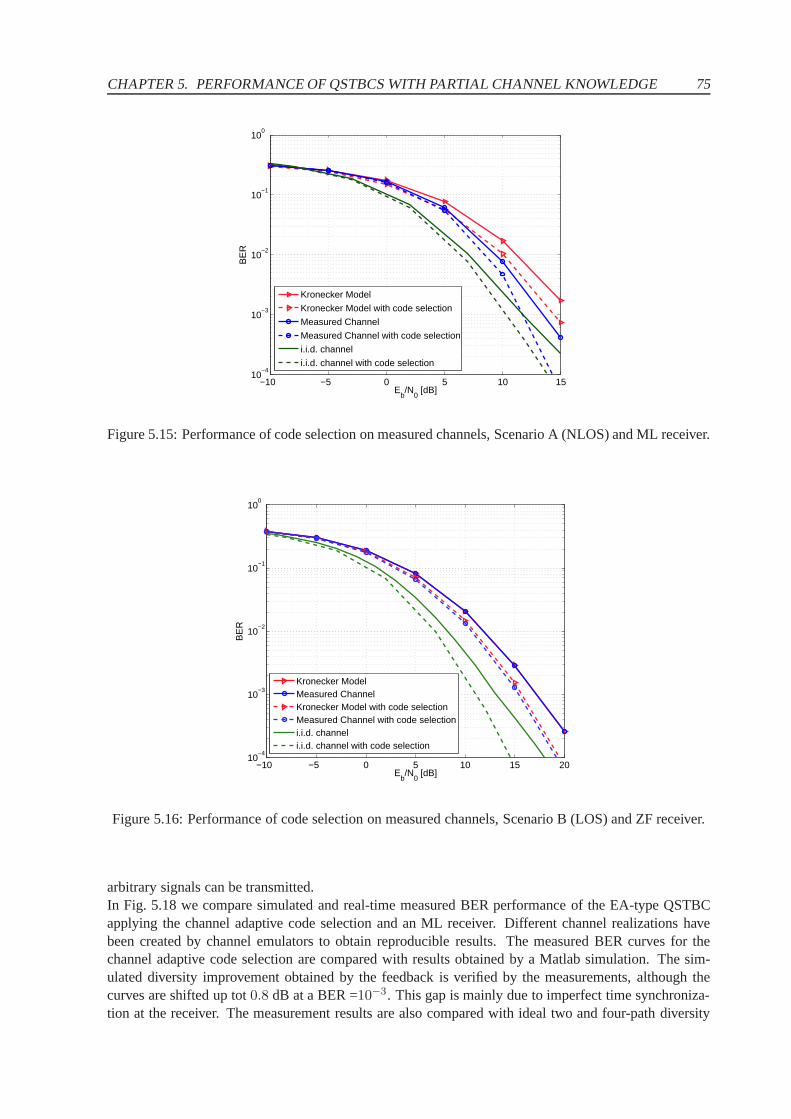
CHAPTER 5. PERFORMANCE OF QSTBCS WITH PARTIAL CHANNEL KNOWLEDGE 75
−10 −5 0 5 10 1510
−4
10−3
10−2
10−1
100
Eb/N
0 [dB]
BE
R
Kronecker Model
Kronecker Model with code selection
Measured Channel
Measured Channel with code selection
i.i.d. channel
i.i.d. channel with code selection
Figure 5.15: Performance of code selection on measured channels, Scenario A (NLOS) and ML receiver.
−10 −5 0 5 10 15 2010
−4
10−3
10−2
10−1
100
Eb/N
0 [dB]
BE
R
Kronecker ModelMeasured ChannelKronecker Model with code selectionMeasured Channel with code selectioni.i.d. channeli.i.d. channel with code selection
Figure 5.16: Performance of code selection on measured channels, Scenario B (LOS) and ZF receiver.
arbitrary signals can be transmitted.In Fig. 5.18 we compare simulated and real-time measured BERperformance of the EA-type QSTBCapplying the channel adaptive code selection and an ML receiver. Different channel realizations havebeen created by channel emulators to obtain reproducible results. The measured BER curves for thechannel adaptive code selection are compared with results obtained by a Matlab simulation. The sim-ulated diversity improvement obtained by the feedback is verified by the measurements, although thecurves are shifted up tot0.8 dB at a BER =10−3. This gap is mainly due to imperfect time synchroniza-tion at the receiver. The measurement results are also compared with ideal two and four-path diversity
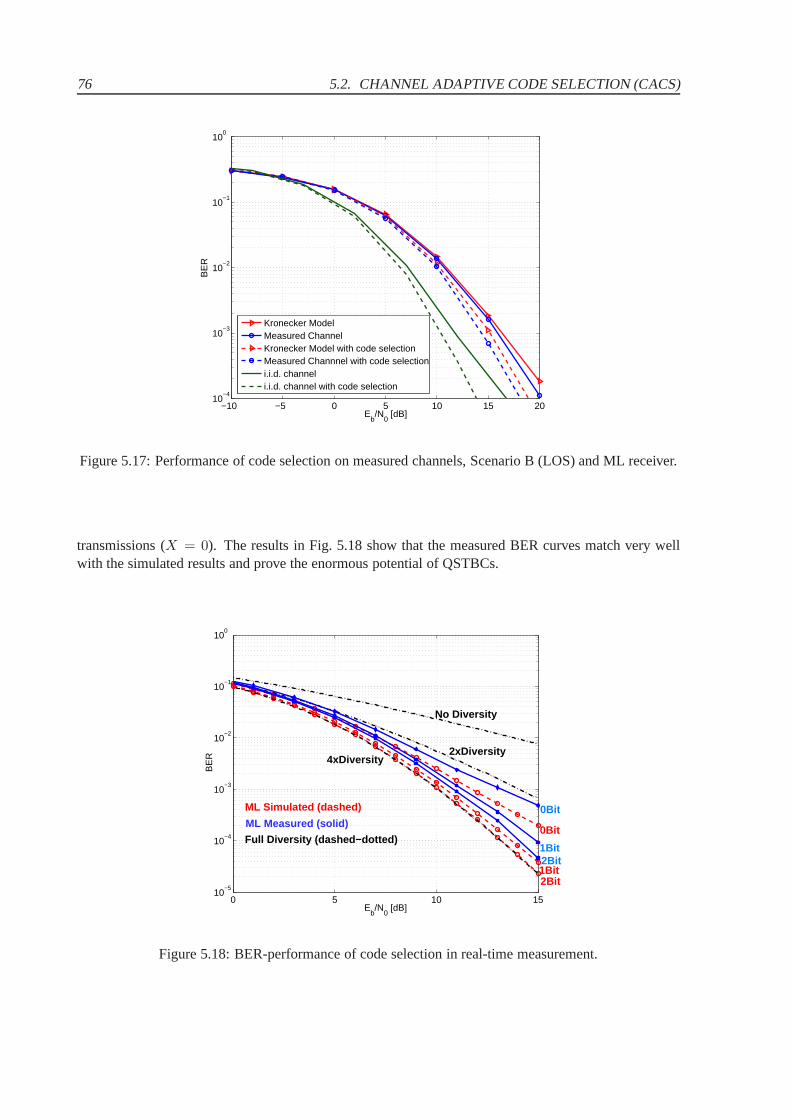
76 5.2. CHANNEL ADAPTIVE CODE SELECTION (CACS)
−10 −5 0 5 10 15 2010
−4
10−3
10−2
10−1
100
Eb/N
0 [dB]
BE
R
Kronecker ModelMeasured ChannelKronecker Model with code selectionMeasured Channnel with code selectioni.i.d. channeli.i.d. channel with code selection
Figure 5.17: Performance of code selection on measured channels, Scenario B (LOS) and ML receiver.
transmissions (X = 0). The results in Fig. 5.18 show that the measured BER curves match very wellwith the simulated results and prove the enormous potentialof QSTBCs.
0 5 10 1510
−5
10−4
10−3
10−2
10−1
100
Eb/N
0 [dB]
BE
R
ML Measured (solid) Full Diversity (dashed−dotted)
No Diversity
2xDiversity 4xDiversity
ML Simulated (dashed)
1Bit
0Bit
2Bit
0Bit
1Bit2Bit
Figure 5.18: BER-performance of code selection in real-time measurement.
CHAPTER 5. PERFORMANCE OF QSTBCS WITH PARTIAL CHANNEL KNOWLEDGE 77
5.3 Channel Adaptive Transmit Antenna Selection (CAAS)
The main impediment in deploying multiple antennas is the additional complexity associated to them.This complexity comes from the following two facts.
1. Increased processing effort.Both transmitter and receiver need to be equipped with powerful signal-processors in order tohandle the algorithmic intricacy introduced by the use of multiple antennas.
2. Multiple radio-frequency (RF) front ends.Thesimultaneousutilization of multiple antennas also implies that the number of costly analog-circuitry elements integrated on both sides of the link is significantly higher compared to the singleantenna case.
Technical advancements in the field of digital signal processor (DSP) design are significantly faster thenin the domain of low cost integration of high frequency analog equipment. Consequently, the needfor more DSP power will eventually become less of a problem. The following quote taken from [79]confirms this conjecture:
“While additional antenna elements (patch or dipole antennas) are usually inexpensive, andthe additional digital signal processing power becomes ever cheaper, the RF elements areexpensive and do not follow Moore’s law.”
One attractive way to reduce the number of RF chains is antenna selection (AS) [74, 75, 76, 77]. Systemsequipped with this capability optimally choose a subset of the available transmit and receive antennasand only process the signals associated with them. This allows to maximally benefit from the multipleantennas within given RF complexity and cost constraints since the diversity order associated with anoptimally selected antenna system is the same as that of the system with all antennas in use.
Obviously, the performance of an AS scheme compared to the non-selective, full complexity systemdepends on the signaling scheme, the receiver structure, the capability of the applied selection algorithmto compute the subset that is best suited (optimum) for the current channel state and the nature of thechannel knowledge.
Generally, three different ways of antenna selection exist:
1. Antenna selection at the receiver only (no feedback information).
2. Antenna selection at the transmitter only (feedback information required).
3. Antenna selection at both ends (feedback information required).
In all of those selection scenarios the computation of the optimum antenna subset is based on estimatesof the channel coefficients as perceived by the receiver. Since channel reciprocity cannot be assumedin general the transmitter cannot do this by itself and needsto be provided with that subset information(closed loop system). This critical requirement is a major drawback of transmit and combined selectionschemes. Furthermore, the information rates of permanently available feedback links are usually verylimited. It is therefore of interest to devise closed loop schemes that can achieve high selection gainswith as little feedback information as possible.
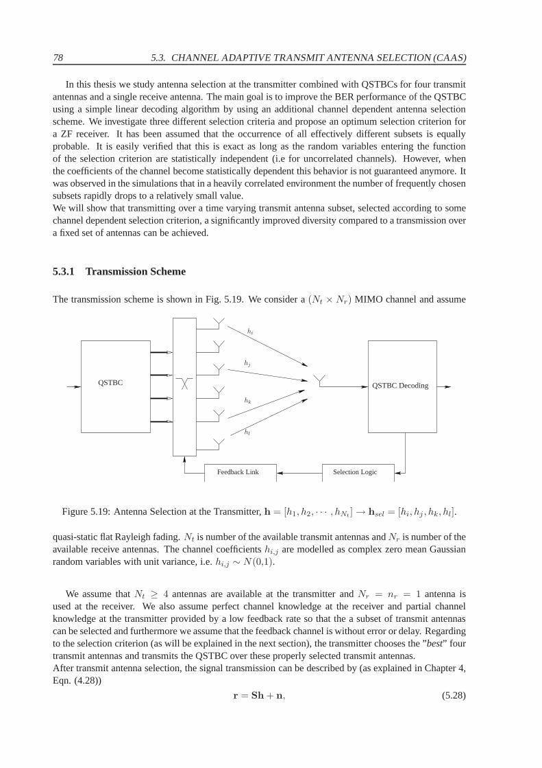
78 5.3. CHANNEL ADAPTIVE TRANSMIT ANTENNA SELECTION (CAAS)
In this thesis we study antenna selection at the transmittercombined with QSTBCs for four transmitantennas and a single receive antenna. The main goal is to improve the BER performance of the QSTBCusing a simple linear decoding algorithm by using an additional channel dependent antenna selectionscheme. We investigate three different selection criteriaand propose an optimum selection criterion fora ZF receiver. It has been assumed that the occurrence of all effectively different subsets is equallyprobable. It is easily verified that this is exact as long as the random variables entering the functionof the selection criterion are statistically independent (i.e for uncorrelated channels). However, whenthe coefficients of the channel become statistically dependent this behavior is not guaranteed anymore. Itwas observed in the simulations that in a heavily correlatedenvironment the number of frequently chosensubsets rapidly drops to a relatively small value.We will show that transmitting over a time varying transmit antenna subset, selected according to somechannel dependent selection criterion, a significantly improved diversity compared to a transmission overa fixed set of antennas can be achieved.
5.3.1 Transmission Scheme
The transmission scheme is shown in Fig. 5.19. We consider a(Nt × Nr) MIMO channel and assume
QSTBC QSTBC Decoding
Feedback Link Selection Logic
hi
hj
hk
hl
Figure 5.19: Antenna Selection at the Transmitter,h = [h1, h2, · · · , hNt ] → hsel = [hi, hj , hk, hl].
quasi-static flat Rayleigh fading.Nt is number of the available transmit antennas andNr is number of theavailable receive antennas. The channel coefficientshi,j are modelled as complex zero mean Gaussianrandom variables with unit variance, i.e.hi,j ∼ N(0,1).
We assume thatNt ≥ 4 antennas are available at the transmitter andNr = nr = 1 antenna isused at the receiver. We also assume perfect channel knowledge at the receiver and partial channelknowledge at the transmitter provided by a low feedback rateso that the a subset of transmit antennascan be selected and furthermore we assume that the feedback channel is without error or delay. Regardingto the selection criterion (as will be explained in the next section), the transmitter chooses the ”best” fourtransmit antennas and transmits the QSTBC over these properly selected transmit antennas.After transmit antenna selection, the signal transmissioncan be described by (as explained in Chapter 4,Eqn. (4.28))
r = Sh + n, (5.28)
CHAPTER 5. PERFORMANCE OF QSTBCS WITH PARTIAL CHANNEL KNOWLEDGE 79
whereS is the QSTBC,r is the (4 × 1) vector of signals received at the receive antenna within foursuccessive time slots andv is the(nr × 1) complex-valued Gaussian noise vector.From the previous chapter we know, that by complex conjugation of some elements ofr, the transmission(5.28) can be reformulated as
y = Hvs + n,
whereHv is an(4 × 4) equivalent virtual channel matrix (EVCM).
On the receiver side we apply a low-complexity ZF receiver. Due to the quasi-orthogonality of theapplied QSTBC the results for this transmission system using a linear receiver differ from the optimummaximum-likelihood (ML) receiver performance. On the other hand, the simple ZF detection approachexhibits very low computational complexity and also benefits from the fact that complex matrix inversionis not necessary. The ZF receiver algorithm leads to
y = (HHv Hv)
−1y = s + (HHv Hv)
−1HHv n. (5.29)
As already has been shown in Chapter 4, Section 4.6.3, Eqn.(4.46) the expression for the instantaneousbit error ratio of QSTBC using the ZF receiver is
BERZF = Eh2,X
{
Q(√
h2(1 − X2)
σ2n
)}
.
In fact, the fading factorh2 as well as the interference parameterX determine the BER performance asalready shown in previous sections. Our optimization criterion will be based on minimizing BER.
5.3.2 Antenna Selection Criteria
The selection process consists of selecting thent ”best suited” antennas (in this section we choosent =4) out ofNt available with channel coefficientshi,j,k,l = (hi, hj , hk, hl)
T ,1 ≤ i < j < k < l ≤ Nt. Theordering of the transmit antenna elements is always set to the default sequence with strictly increasingindicesi, j, k, l.We assume that the receiver has perfect channel knowledge and that it returns some channel informationto the transmitter in form of some control bits. At the transmitter, four out ofNt transmit antennas areselected for transmitting the QSTBC. In total, there are
qeff =
(
Nt
4
)
possibilities to select a subset ofnt = 4 transmit antennas out of a set ofNt available antennas andtherefore
bfeedback =⌈
log2(qeff)⌉
=
⌈
log2
[(
Nt
4
)]
⌉
bits
have to be returned to inform the transmitter which transmitantenna subset should be used. We assumethat the receiver knows allNt complex channel gainsh1 to hNt and finds the best subset ofnt = 4transmit antennas to be used, according to one of the three optimization criteria discussed below. Then,the receiver provides the transmitter with this information via a low-rate feedback channel (we assumethat the channel varies slowly and is constant during each QSTBC block).
From the previous section, we know that the self-interference parameterX and the channel gainh2 need to be jointly considered when”the best” antenna subset has to be determined. In fact, our
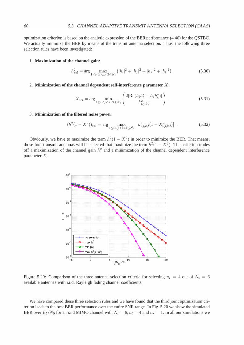
80 5.3. CHANNEL ADAPTIVE TRANSMIT ANTENNA SELECTION (CAAS)
optimization criterion is based on the analytic expressionof the BER performance (4.46) for the QSTBC.We actually minimize the BER by means of the transmit antennaselection. Thus, the following threeselection rules have been investigated:
1. Maximization of the channel gain:
h2sel = arg max
1≤i<j<k<l≤Nt
(
|hi|2 + |hj |2 + |hk|2 + |hl|2)
. (5.30)
2. Minimization of the channel dependent self-interference parameter X:
Xsel = arg min1≤i<j<k<l≤Nt
(
2|Re(hih∗l − hjh
∗k)|
h2i,j,k,l
)
. (5.31)
3. Minimization of the filtered noise power:
(h2(1 − X2))sel = arg max1≤i<j<k<l≤Nt
[
h2i,j,k,l(1 − X2
i,j,k,l)]
. (5.32)
Obviously, we have to maximize the termh2(1 − X2) in order to minimize the BER. That means,those four transmit antennas will be selected that maximizethe termh2(1 − X2). This criterion tradesoff a maximization of the channel gainh2 and a minimization of the channel dependent interferenceparameterX.
−5 0 5 10 15 2010
−6
10−5
10−4
10−3
10−2
10−1
100
Eb/N
0 [dB]
BE
R
no selection
max h2
min |X|
max h2(1−X2)
Figure 5.20: Comparison of the three antenna selection criteria for selectingnt = 4 out of Nt = 6available antennas with i.i.d. Rayleigh fading channel coefficients.
We have compared these three selection rules and we have found that the third joint optimization cri-terion leads to the best BER performance over the entire SNR range. In Fig. 5.20 we show the simulatedBER overEb/N0 for an i.i.d MIMO channel withNt = 6, nt = 4 andnr = 1. In all our simulations we
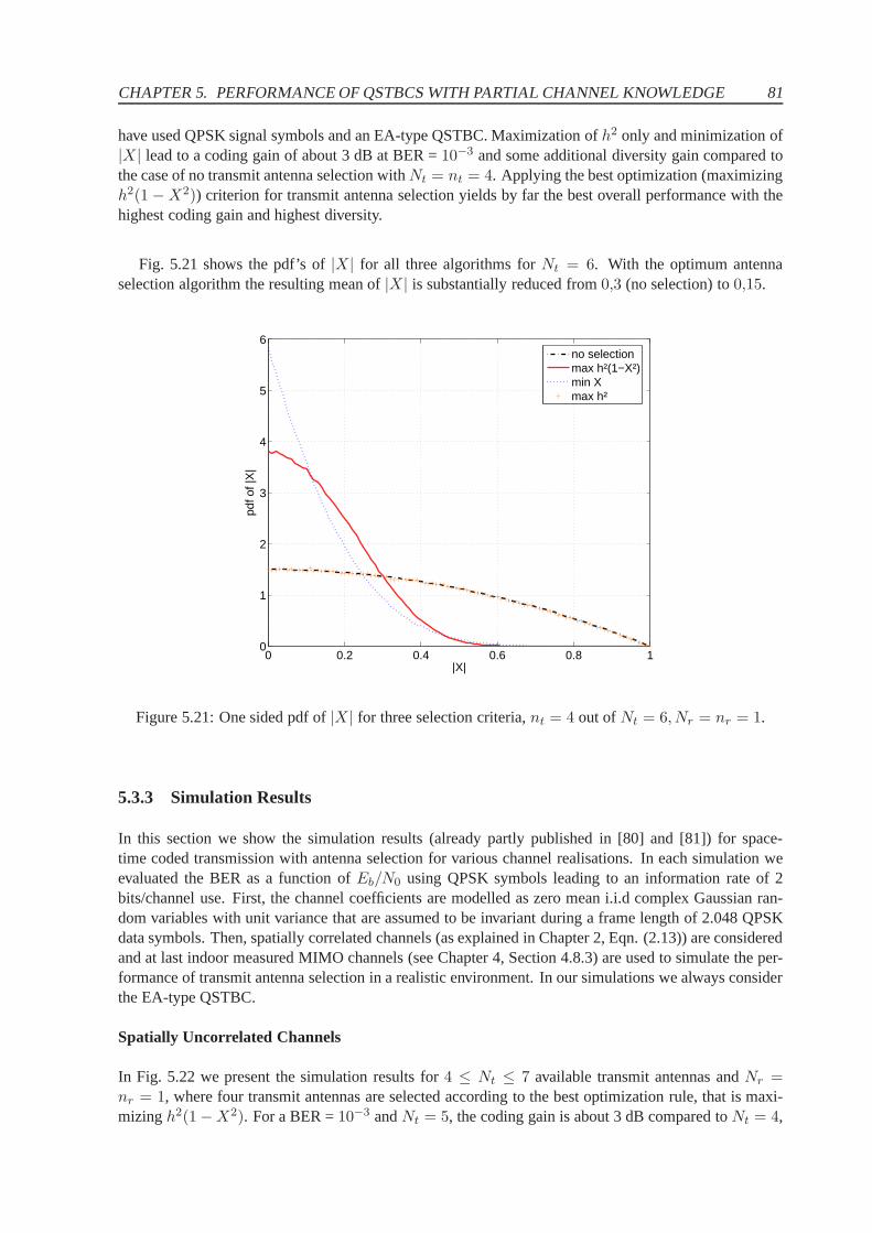
CHAPTER 5. PERFORMANCE OF QSTBCS WITH PARTIAL CHANNEL KNOWLEDGE 81
have used QPSK signal symbols and an EA-type QSTBC. Maximization of h2 only and minimization of|X| lead to a coding gain of about 3 dB at BER =10−3 and some additional diversity gain compared tothe case of no transmit antenna selection withNt = nt = 4. Applying the best optimization (maximizingh2(1 − X2)) criterion for transmit antenna selection yields by far thebest overall performance with thehighest coding gain and highest diversity.
Fig. 5.21 shows the pdf’s of|X| for all three algorithms forNt = 6. With the optimum antennaselection algorithm the resulting mean of|X| is substantially reduced from0,3 (no selection) to0,15.
0 0.2 0.4 0.6 0.8 10
1
2
3
4
5
6
|X|
pdf o
f |X
|
no selection max h²(1−X²)min Xmax h²
Figure 5.21: One sided pdf of|X| for three selection criteria,nt = 4 out ofNt = 6, Nr = nr = 1.
5.3.3 Simulation Results
In this section we show the simulation results (already partly published in [80] and [81]) for space-time coded transmission with antenna selection for variouschannel realisations. In each simulation weevaluated the BER as a function ofEb/N0 using QPSK symbols leading to an information rate of 2bits/channel use. First, the channel coefficients are modelled as zero mean i.i.d complex Gaussian ran-dom variables with unit variance that are assumed to be invariant during a frame length of 2.048 QPSKdata symbols. Then, spatially correlated channels (as explained in Chapter 2, Eqn. (2.13)) are consideredand at last indoor measured MIMO channels (see Chapter 4, Section 4.8.3) are used to simulate the per-formance of transmit antenna selection in a realistic environment. In our simulations we always considerthe EA-type QSTBC.
Spatially Uncorrelated Channels
In Fig. 5.22 we present the simulation results for4 ≤ Nt ≤ 7 available transmit antennas andNr =nr = 1, where four transmit antennas are selected according to thebest optimization rule, that is maxi-mizingh2(1 − X2). For a BER =10−3 andNt = 5, the coding gain is about 3 dB compared toNt = 4,
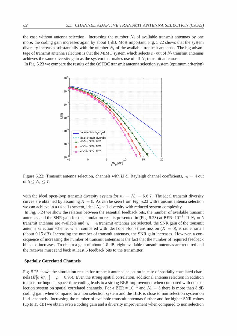
82 5.3. CHANNEL ADAPTIVE TRANSMIT ANTENNA SELECTION (CAAS)
the case without antenna selection. Increasing the numberNt of available transmit antennas by onemore, the coding gain increases again by about 1 dB. Most important, Fig. 5.22 shows that the systemdiversity increases substantially with the numberNt of the available transmit antennas. The big advan-tage of transmit antenna selection is that the MIMO system which selectsnt out ofNt transmit antennasachieves the same diversity gain as the system that makes useof all Nt transmit antennas.In Fig. 5.23 we compare the results of the QSTBC transmit antenna selection system (optimum criterion)
−5 0 5 10 15 2010
−6
10−5
10−4
10−3
10−2
10−1
100
Eb/N
0 [dB]
BE
R
no selection Nt=n
t=4
ideal 4−path diversityCAAS, N
t=5, n
t=4
CAAS, Nt=6, n
t=4
CAAS, Nt=7, n
t=4
Figure 5.22: Transmit antenna selection, channels with i.i.d. Rayleigh channel coefficients,nt = 4 outof 5 ≤ Nt ≤ 7.
with the ideal open-loop transmit diversity system fornt = Nt = 5,6,7. The ideal transmit diversitycurves are obtained by assumingX = 0. As can be seen from Fig. 5.23 with transmit antenna selectionwe can achieve in a(4 × 1) system, idealNt × 1 diversity with reduced system complexity.In Fig. 5.24 we show the relation between the essential feedback bits, the number of available transmit
antennas and the SNR gain for the simulation results presented in (Fig. 5.23) at BER=10−4. If Nt = 5transmit antennas are available andnt = 4 transmit antennas are selected, the SNR gain of the transmitantenna selection scheme, when compared with ideal open-loop transmission (X = 0), is rather small(about 0.15 dB). Increasing the number of transmit antennas, the SNR gain increases. However, a con-sequence of increasing the number of transmit antennas is the fact that the number of required feedbackbits also increases. To obtain a gain of about1.5 dB, eight available transmit antennas are required andthe receiver must send back at least 6 feedback bits to the transmitter.
Spatially Correlated Channels
Fig. 5.25 shows the simulation results for transmit antennaselection in case of spatially correlated chan-nels (E[hih
∗i+1] = ρ = 0,95). Even the strong spatial correlation, additional antennaselection in addition
to quasi-orthogonal space-time coding leads to a strong BERimprovement when compared with non se-lection system on spatial correlated channels. For a BER =10−3 andNt = 5 there is more than5 dBcoding gain when compared to a non selection system and the BER is close to non selection system oni.i.d. channels. Increasing the number of available transmit antennas further and for higher SNR values(up to 15 dB) we obtain even a coding gain and a diversity improvement when compared to non selection
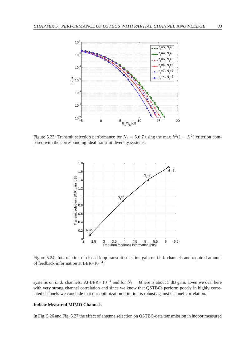
CHAPTER 5. PERFORMANCE OF QSTBCS WITH PARTIAL CHANNEL KNOWLEDGE 83
−5 0 5 10 15 2010
−6
10−5
10−4
10−3
10−2
10−1
100
Eb/N
0 [dB]
BE
R
nt=5, N
t=5
nt=4, N
t=5
nt=6, N
t=6
nt=4, N
t=6
nt=7, N
t=7
nt=4, N
t=7
Figure 5.23: Transmit selection performance forNt = 5,6,7 using the maxh2(1 − X2) criterion com-pared with the corresponding ideal transmit diversity systems.
2 2.5 3 3.5 4 4.5 5 5.5 6 6.50
0.2
0.4
0.6
0.8
1
1.2
1.4
1.6
1.8
Required feedback information [bits]
Tra
nsm
it se
lect
ion
SN
R g
ain
[dB
]
Nt=5
Nt=6
Nt=7
Nt=8
Figure 5.24: Interrelation of closed loop transmit selection gain on i.i.d. channels and required amountof feedback information at BER=10−4.
systems on i.i.d. channels. At BER=10−4 and forNt = 6there is about3 dB gain. Even we deal herewith very strong channel correlation and since we know that QSTBCs perform poorly in highly corre-lated channels we conclude that our optimization criterionis robust against channel correlation.
Indoor Measured MIMO Channels
In Fig. 5.26 and Fig. 5.27 the effect of antenna selection on QSTBC-data transmission in indoor measured
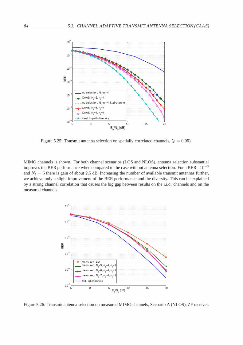
84 5.3. CHANNEL ADAPTIVE TRANSMIT ANTENNA SELECTION (CAAS)
−5 0 5 10 15 2010
−6
10−5
10−4
10−3
10−2
10−1
100
Eb/N
0 [dB]
BE
R
no selection, Nt=n
t=4
CAAS, Nt=5, n
t=4
no selection, Nt=n
t=4, i.i.d channel
CAAS, Nt=6, n
t=4
CAAS, Nt=7, n
t=4
ideal 4−path diversity
Figure 5.25: Transmit antenna selection on spatially correlated channels, (ρ = 0,95).
MIMO channels is shown. For both channel scenarios (LOS and NLOS), antenna selection substantialimproves the BER performance when compared to the case without antenna selection. For a BER=10−3
andNt = 5 there is gain of about2,5 dB. Increasing the number of available transmit antennas further,we achieve only a slight improvement of the BER performance and the diversity. This can be explainedby a strong channel correlation that causes the big gap between results on the i.i.d. channels and on themeasured channels.
−5 0 5 10 15 2010
−5
10−4
10−3
10−2
10−1
100
Eb/N
0 [dB]
BE
R
measured, 4x1measured, N
t=5, n
t=4, n
r=1
measured, Nt=6, n
t=4, n
r=1
measured, Nt=7, n
t=4, n
r=1
4x1, iid channels
Figure 5.26: Transmit antenna selection on measured MIMO channels, Scenario A (NLOS), ZF receiver.
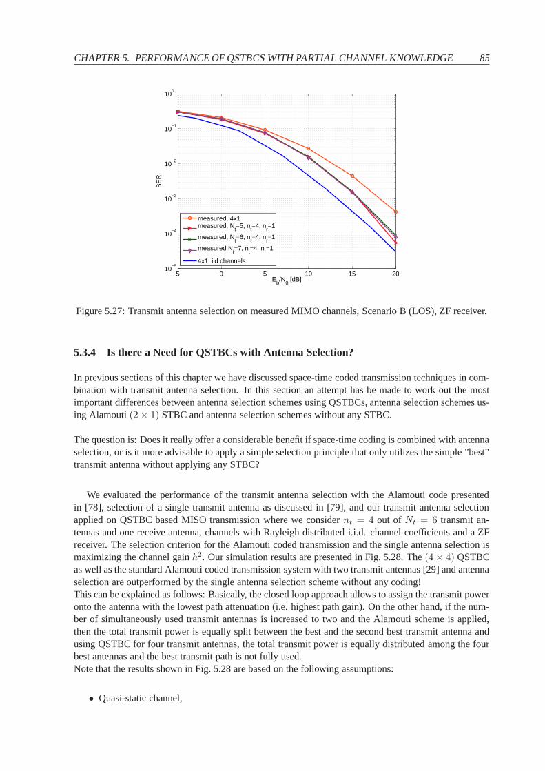
CHAPTER 5. PERFORMANCE OF QSTBCS WITH PARTIAL CHANNEL KNOWLEDGE 85
−5 0 5 10 15 2010
−5
10−4
10−3
10−2
10−1
100
Eb/N
0 [dB]
BE
R
measured, 4x1measured, N
t=5, n
t=4, n
r=1
measured, Nt=6, n
t=4, n
r=1
measured Nt=7, n
t=4, n
r=1
4x1, iid channels
Figure 5.27: Transmit antenna selection on measured MIMO channels, Scenario B (LOS), ZF receiver.
5.3.4 Is there a Need for QSTBCs with Antenna Selection?
In previous sections of this chapter we have discussed space-time coded transmission techniques in com-bination with transmit antenna selection. In this section an attempt has be made to work out the mostimportant differences between antenna selection schemes using QSTBCs, antenna selection schemes us-ing Alamouti(2 × 1) STBC and antenna selection schemes without any STBC.
The question is: Does it really offer a considerable benefit if space-time coding is combined with antennaselection, or is it more advisable to apply a simple selection principle that only utilizes the simple ”best”transmit antenna without applying any STBC?
We evaluated the performance of the transmit antenna selection with the Alamouti code presentedin [78], selection of a single transmit antenna as discussedin [79], and our transmit antenna selectionapplied on QSTBC based MISO transmission where we considernt = 4 out of Nt = 6 transmit an-tennas and one receive antenna, channels with Rayleigh distributed i.i.d. channel coefficients and a ZFreceiver. The selection criterion for the Alamouti coded transmission and the single antenna selection ismaximizing the channel gainh2. Our simulation results are presented in Fig. 5.28. The(4 × 4) QSTBCas well as the standard Alamouti coded transmission system with two transmit antennas [29] and antennaselection are outperformed by the single antenna selectionscheme without any coding!This can be explained as follows: Basically, the closed loopapproach allows to assign the transmit poweronto the antenna with the lowest path attenuation (i.e. highest path gain). On the other hand, if the num-ber of simultaneously used transmit antennas is increased to two and the Alamouti scheme is applied,then the total transmit power is equally split between the best and the second best transmit antenna andusing QSTBC for four transmit antennas, the total transmit power is equally distributed among the fourbest antennas and the best transmit path is not fully used.Note that the results shown in Fig. 5.28 are based on the following assumptions:
• Quasi-static channel,
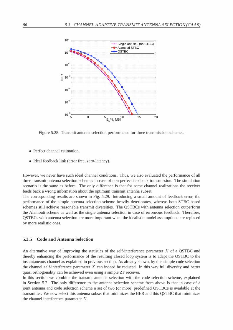
86 5.3. CHANNEL ADAPTIVE TRANSMIT ANTENNA SELECTION (CAAS)
−5 0 5 10 15 2010
−6
10−5
10−4
10−3
10−2
10−1
100
Eb/N
0 [dB]
BE
R
Single ant. sel. (no STBC)Alamouti STBCQSTBC
Figure 5.28: Transmit antenna selection performance for three transmission schemes.
• Perfect channel estimation,
• Ideal feedback link (error free, zero-latency).
However, we never have such ideal channel conditions. Thus,we also evaluated the performance of allthree transmit antenna selection schemes in case of non perfect feedback transmission. The simulationscenario is the same as before. The only difference is that for some channel realizations the receiverfeeds back a wrong information about the optimum transmit antenna subset.The corresponding results are shown in Fig. 5.29. Introducing a small amount of feedback error, theperformance of the simple antenna selection scheme heavilydeteriorates, whereas both STBC basedschemes still achieve reasonable transmit diversities. The QSTBCs with antenna selection outperformthe Alamouti scheme as well as the single antenna selection in case of erroneous feedback. Therefore,QSTBCs with antenna selection are more important when the idealistic model assumptions are replacedby more realistic ones.
5.3.5 Code and Antenna Selection
An alternative way of improving the statistics of the self-interference parameterX of a QSTBC andthereby enhancing the performance of the resulting closed loop system is to adapt the QSTBC to theinstantaneous channel as explained in previous section. Asalready shown, by this simple code selectionthe channel self-interference parameterX can indeed be reduced. In this way full diversity and betterquasi orthogonality can be achieved even using a simple ZF receiver.In this section we combine the transmit antenna selection with the code selection scheme, explainedin Section 5.2. The only difference to the antenna selectionscheme from above is that in case of ajoint antenna and code selection scheme a set of two (or more)predefined QSTBCs is available at thetransmitter. We now select this antenna subset that minimizes the BER and this QSTBC that minimizesthe channel interference parameterX.
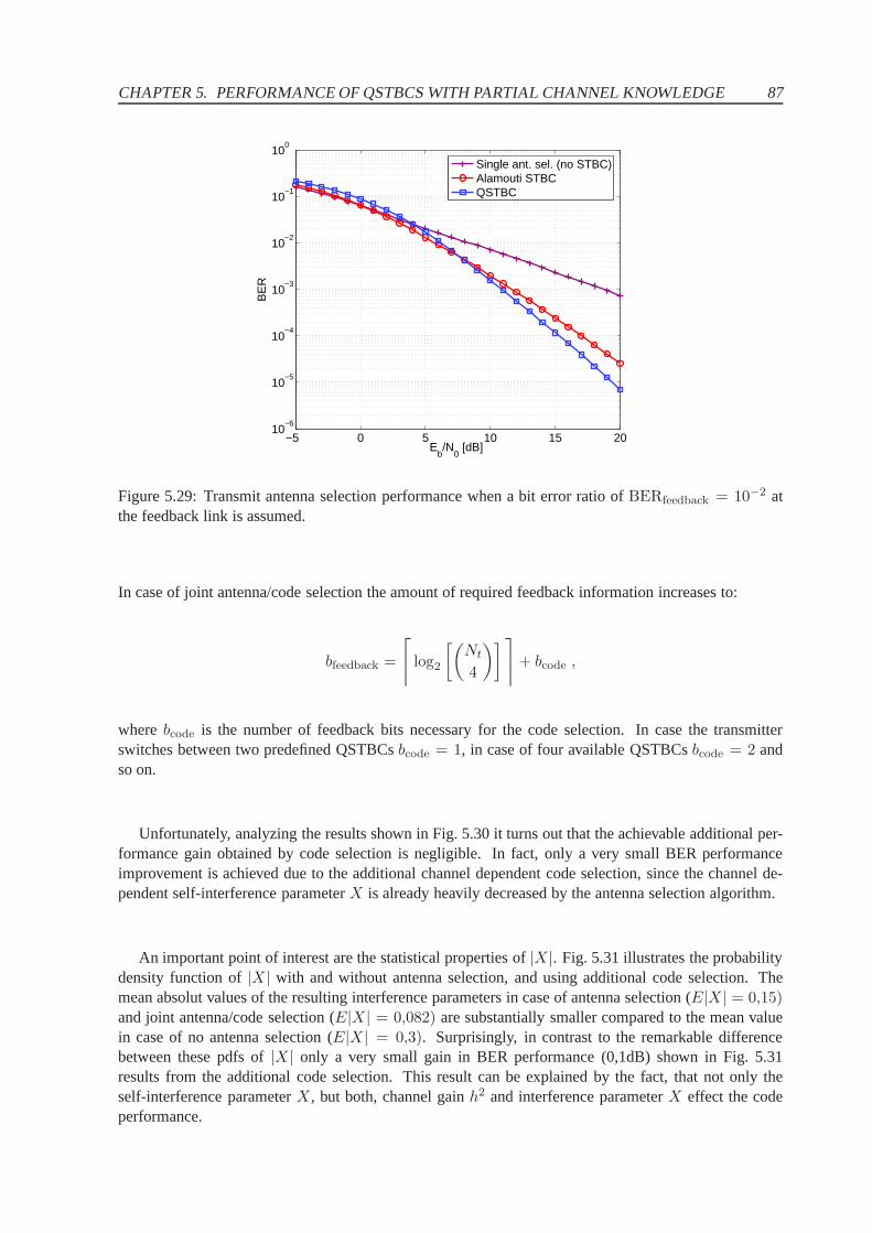
CHAPTER 5. PERFORMANCE OF QSTBCS WITH PARTIAL CHANNEL KNOWLEDGE 87
−5 0 5 10 15 2010
−6
10−5
10−4
10−3
10−2
10−1
100
Eb/N
0 [dB]
BE
R
Single ant. sel. (no STBC)Alamouti STBCQSTBC
Figure 5.29: Transmit antenna selection performance when abit error ratio ofBERfeedback = 10−2 atthe feedback link is assumed.
In case of joint antenna/code selection the amount of required feedback information increases to:
bfeedback =
⌈
log2
[(
Nt
4
)]
⌉
+ bcode ,
wherebcode is the number of feedback bits necessary for the code selection. In case the transmitterswitches between two predefined QSTBCsbcode = 1, in case of four available QSTBCsbcode = 2 andso on.
Unfortunately, analyzing the results shown in Fig. 5.30 it turns out that the achievable additional per-formance gain obtained by code selection is negligible. In fact, only a very small BER performanceimprovement is achieved due to the additional channel dependent code selection, since the channel de-pendent self-interference parameterX is already heavily decreased by the antenna selection algorithm.
An important point of interest are the statistical properties of|X|. Fig. 5.31 illustrates the probabilitydensity function of|X| with and without antenna selection, and using additional code selection. Themean absolut values of the resulting interference parameters in case of antenna selection (E|X| = 0,15)and joint antenna/code selection (E|X| = 0,082) are substantially smaller compared to the mean valuein case of no antenna selection (E|X| = 0,3). Surprisingly, in contrast to the remarkable differencebetween these pdfs of|X| only a very small gain in BER performance (0,1dB) shown in Fig. 5.31results from the additional code selection. This result canbe explained by the fact, that not only theself-interference parameterX, but both, channel gainh2 and interference parameterX effect the codeperformance.
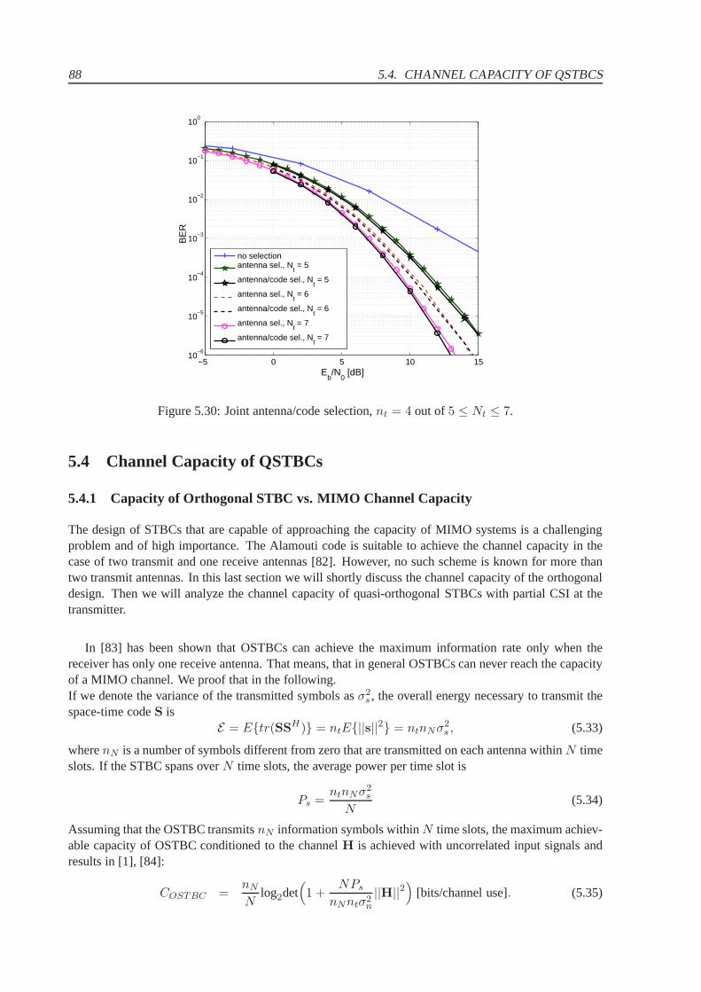
88 5.4. CHANNEL CAPACITY OF QSTBCS
−5 0 5 10 1510
−6
10−5
10−4
10−3
10−2
10−1
100
Eb/N
0 [dB]
BE
R
no selectionantenna sel., N
t = 5
antenna/code sel., Nt = 5
antenna sel., Nt = 6
antenna/code sel., Nt = 6
antenna sel., Nt = 7
antenna/code sel., Nt = 7
Figure 5.30: Joint antenna/code selection,nt = 4 out of5 ≤ Nt ≤ 7.
5.4 Channel Capacity of QSTBCs
5.4.1 Capacity of Orthogonal STBC vs. MIMO Channel Capacity
The design of STBCs that are capable of approaching the capacity of MIMO systems is a challengingproblem and of high importance. The Alamouti code is suitable to achieve the channel capacity in thecase of two transmit and one receive antennas [82]. However,no such scheme is known for more thantwo transmit antennas. In this last section we will shortly discuss the channel capacity of the orthogonaldesign. Then we will analyze the channel capacity of quasi-orthogonal STBCs with partial CSI at thetransmitter.
In [83] has been shown that OSTBCs can achieve the maximum information rate only when thereceiver has only one receive antenna. That means, that in general OSTBCs can never reach the capacityof a MIMO channel. We proof that in the following.If we denote the variance of the transmitted symbols asσ2
s , the overall energy necessary to transmit thespace-time codeS is
E = E{tr(SSH)} = ntE{||s||2} = ntnNσ2s , (5.33)
wherenN is a number of symbols different from zero that are transmitted on each antenna withinN timeslots. If the STBC spans overN time slots, the average power per time slot is
Ps =ntnNσ2
s
N(5.34)
Assuming that the OSTBC transmitsnN information symbols withinN time slots, the maximum achiev-able capacity of OSTBC conditioned to the channelH is achieved with uncorrelated input signals andresults in [1], [84]:
COSTBC =nN
Nlog2det
(
1 +NPs
nNntσ2n
||H||2)
[bits/channel use]. (5.35)
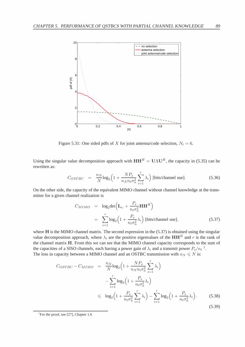
CHAPTER 5. PERFORMANCE OF QSTBCS WITH PARTIAL CHANNEL KNOWLEDGE 89
0 0.2 0.4 0.6 0.8 10
2
4
6
8
10
|X|
pdf o
f |X
|
no selectionantenna selectionjoint antenna/code selection
Figure 5.31: One sided pdfs ofX for joint antenna/code selection,Nt = 6.
Using the singular value decomposition approach withHHH = UΛUH , the capacity in (5.35) can berewritten as:
COSTBC =nN
Nlog2
(
1 +NPs
nNntσ2n
r∑
i=1
λi
)
[bits/channel use]. (5.36)
On the other side, the capacity of the equivalent MIMO channel without channel knowledge at the trans-mitter for a given channel realization is
CMIMO = log2det(
Inr +Ps
ntσ2n
HHH)
=r∑
i=1
log2
(
1 +Ps
ntσ2n
λi
)
[bits/channel use], (5.37)
whereH is the MIMO channel matrix. The second expression in the (5.37) is obtained using the singularvalue decomposition approach, whereλi are the positive eigenvalues of theHHH andr is the rank ofthe channel matrixH. From this we can see that the MIMO channel capacity corresponds to the sum ofthe capacities of a SISO channels, each having a power gain ofλi and a transmit powerPs/nt
1.The loss in capacity between a MIMO channel and an OSTBC transmission withnN 6 N is:
COSTBC − CMIMO =nN
Nlog2
(
1 +NPs
nNntσ2n
r∑
i=1
λi
)
−r∑
i=1
log2
(
1 +Ps
ntσ2n
λi
)
6 log2
(
1 +Ps
ntσ2n
r∑
i=1
λi
)
−r∑
i=1
log2
(
1 +Ps
ntσ2n
λi
)
. (5.38)
(5.39)1For the proof, see [27], Chapter 1.6
90 5.4. CHANNEL CAPACITY OF QSTBCS
With the property
a log(1 + x/a) 6 log(1 + x), for 0 < a 6 1 and x > 0, (5.40)
and
log
(
1 +∑
i
xi
)
6∑
i
log(1 + xi), for x > 0. (5.41)
we obtain
COSTBC − CMIMO 6 0. (5.42)
The equality sign in (5.38) and (5.42) hold true if and only ifnN = N and the channel rank is one(r = 1). This condition is only fulfilled by the Alamouti full rate,full diversity code. Therefore, from(5.38) we can conclude that the orthogonal design cannot reach the MIMO channel capacity, except forthe case whennN = N and the channel rank is one (r = 1) [82].
For the case of a MISO system (nr = 1, nt > nr), the channel matrix is a row matrixH =(h1, h2, · · · , hnt). With HHH =
∑ntj=1 |hj |2 eqn. (5.37) specializes into
CMISO = log2
(
1 +Ps
ntσ2n
nt∑
j
|hj |2)
[bits/channel use]. (5.43)
5.4.2 Capacity of QSTBCs with No Channel State Information at the Transmitter
Since we know that the eigenvalues of a QSTBCs induced equivalent virtual channel matrixHv areλ1,2 = h2(1 + X) andλ3,4 = h2(1 − X) (4.63) the capacity of the QSTBCs for four transmit antennas(when the channel is unknown at the transmitter) can be written as
CQSTBC =1
4log2det
(
1 +Ps
4σ2n
HvHvH)
=1
4· 2 ·
2∑
i=1
log2
(
1 +Ps
4σ2n
λi
)
=1
2
{
log2
(
1 +Ps
4σ2n
h2(1 + X))
+log2
(
1 +Ps
4σ2n
h2(1 − X))}
[bits/channel use]. (5.44)
If the channel dependent interference parameterX vanishes, the channel capacity of a QSTBC schemebecomes
CQSTBCX=0= log2
(
1 +Ps
4σ2n
r∑
j
|hj |2)
[bits/channel use]. (5.45)
This is the ideal channel capacity of a rate-one orthogonal STBC for four transmit antennas and onereceive antenna with uniformly distributed signal power and a given channel realization [84]. However,such a rate-one code does not exist for an open-loop transmission scheme with more than two transmitantennas. Therefore a QSTBC for four transmit antennas and using one receive antenna cannot reach theMISO channel capacity (5.43).
CHAPTER 5. PERFORMANCE OF QSTBCS WITH PARTIAL CHANNEL KNOWLEDGE 91
5.4.3 Capacity of QSTBCs with Channel State Information at the Transmitter
As has been explained in the previous sections, when partialCSI is returned to the transmitter the QST-BCs performance can be substantially improved. In the previous sections, we have shown, that for bothclosed-loop transmission schemes, the channel dependent interference parameterX is approximatelyzero. Thus the channel capacity for QSTBC in code selection transmission scheme withX ≈ 0 can bewritten as:
CQSTBCCS≤ log2
(
1 +Ps
4σ2n
h2)
[bits/channel use] (5.46)
and for the space-time coded transmission in antenna selected MIMO system gain, withX ≈ 0 andh2
sel =∑
j max|hj |2, j = 1, 2, · · · , 4, the channel capacity is given by
CQSTBCTAS≤ log2
(
1 +Ps
4σ2n
h2sel
)
[bits/channel use], (5.47)
whereh2sel is the channel gain from the optimum selected antenna subset. From the Equation (5.47), it
is obvious that the channel capacity of QSTBC with CSI is equal to the MISO channel capacity withoutCSI. We approve this with simulation results given in next section.
5.4.4 Simulation Results
We simulated a3% outage capacity of the EA-type QSTBC with code selection (Fig. 5.32) and withtransmit antenna selection (Fig. 5.33). The channel coefficients are chosen as Gaussian random variableswith unit variance. The outage values are computed based on10.000 independent runs. The results arecompared with the capacity of an ideal open-loop(4 × 1) transmission scheme Eqn. (5.45) and with thechannel capacity of QSTBC without CSI at the transmitter (Eqn. (5.44)).
For low SNR values (up to10 dB) we have not any improvement of the outage capacity applyingcode selection at the transmitter (Fig. 5.32). In the higherSNR range, there is only a small improvementof the outage capacity, about0,2 dB at3 bits/channel use. Even with two bits feedback returned fromthereceiver to the transmitter we do not achieve ideal(4 × 1) open-loop transmission scheme.
From Fig. 5.33 we can observe that QSTBC with transmit antenna selection achieves much higheroutage capacity than QSTBC with code selection. The performance gain between the outage capacityof a transmit antenna selection system whenNt = 5 transmit antennas are available andnt = 4 areselected, compared to the(4× 1) QSTBC without CSI at the transmitter is approximately4,5 dB gain at3 bits/channel use. Increasing the number of the available transmit antennas further, the channel capacityincreases up to1 dB per additional antenna and it remains constant for higherSNR values. It is im-portant to observe, that the outage capacity of the transmitantenna selection system is above the outagecapacity of the ideal open-loop transmission scheme. This is due to the fact that exploiting the CSI atthe transmitter only ”optimum” antennas are used for the data transmission. Obviously, transmit antennaselection not only reduces the complexity of MIMO systems having Nt transmit antennas available, butalso improves the capacity of the MIMO systems at the cost of aminimal amount of feedback.
In Fig. 5.34 we demonstrate that the channel capacity of a QSTBC with CSI at the transmitter can beseen as a MISO channel capacity without any CSI at the transmitter. We compare the outage capacity ofchannel adaptive code selection (one bit feedback) and channel adaptive antenna selection (nt = 4 out
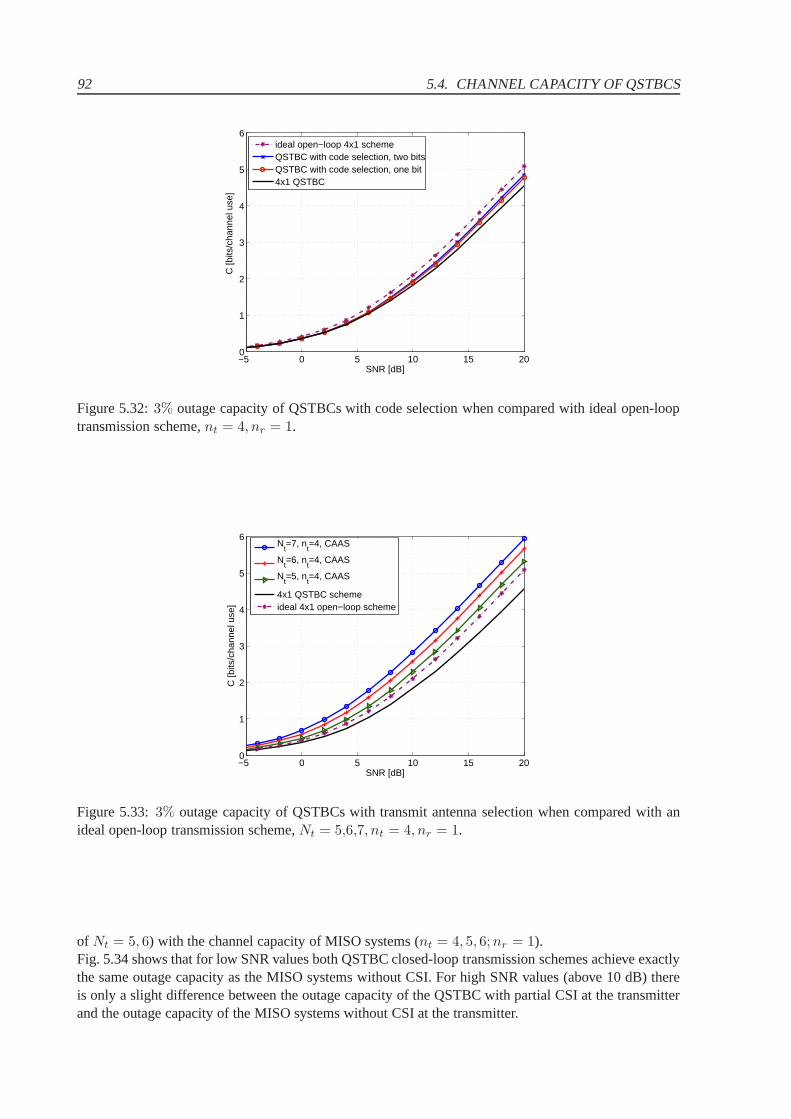
92 5.4. CHANNEL CAPACITY OF QSTBCS
−5 0 5 10 15 200
1
2
3
4
5
6
SNR [dB]
C [b
its/c
hann
el u
se]
ideal open−loop 4x1 schemeQSTBC with code selection, two bitsQSTBC with code selection, one bit4x1 QSTBC
Figure 5.32:3% outage capacity of QSTBCs with code selection when comparedwith ideal open-looptransmission scheme,nt = 4, nr = 1.
−5 0 5 10 15 200
1
2
3
4
5
6
SNR [dB]
C [b
its/c
hann
el u
se]
Nt=7, n
t=4, CAAS
Nt=6, n
t=4, CAAS
Nt=5, n
t=4, CAAS
4x1 QSTBC schemeideal 4x1 open−loop scheme
Figure 5.33:3% outage capacity of QSTBCs with transmit antenna selection when compared with anideal open-loop transmission scheme,Nt = 5,6,7, nt = 4, nr = 1.
of Nt = 5, 6) with the channel capacity of MISO systems (nt = 4, 5, 6;nr = 1).Fig. 5.34 shows that for low SNR values both QSTBC closed-loop transmission schemes achieve exactlythe same outage capacity as the MISO systems without CSI. Forhigh SNR values (above 10 dB) thereis only a slight difference between the outage capacity of the QSTBC with partial CSI at the transmitterand the outage capacity of the MISO systems without CSI at thetransmitter.
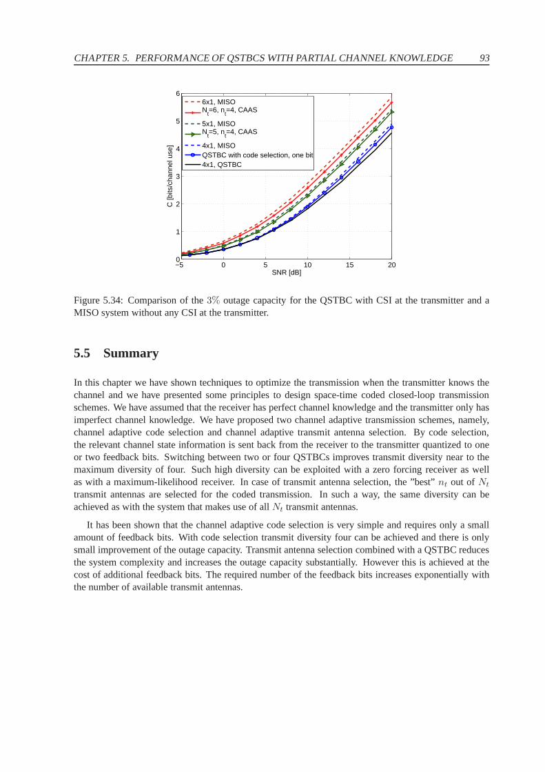
CHAPTER 5. PERFORMANCE OF QSTBCS WITH PARTIAL CHANNEL KNOWLEDGE 93
−5 0 5 10 15 200
1
2
3
4
5
6
SNR [dB]
C [b
its/c
hann
el u
se]
6x1, MISON
t=6, n
t=4, CAAS
5x1, MISON
t=5, n
t=4, CAAS
4x1, MISOQSTBC with code selection, one bit4x1, QSTBC
Figure 5.34: Comparison of the3% outage capacity for the QSTBC with CSI at the transmitter andaMISO system without any CSI at the transmitter.
5.5 Summary
In this chapter we have shown techniques to optimize the transmission when the transmitter knows thechannel and we have presented some principles to design space-time coded closed-loop transmissionschemes. We have assumed that the receiver has perfect channel knowledge and the transmitter only hasimperfect channel knowledge. We have proposed two channel adaptive transmission schemes, namely,channel adaptive code selection and channel adaptive transmit antenna selection. By code selection,the relevant channel state information is sent back from thereceiver to the transmitter quantized to oneor two feedback bits. Switching between two or four QSTBCs improves transmit diversity near to themaximum diversity of four. Such high diversity can be exploited with a zero forcing receiver as wellas with a maximum-likelihood receiver. In case of transmit antenna selection, the ”best”nt out of Nt
transmit antennas are selected for the coded transmission.In such a way, the same diversity can beachieved as with the system that makes use of allNt transmit antennas.
It has been shown that the channel adaptive code selection isvery simple and requires only a smallamount of feedback bits. With code selection transmit diversity four can be achieved and there is onlysmall improvement of the outage capacity. Transmit antennaselection combined with a QSTBC reducesthe system complexity and increases the outage capacity substantially. However this is achieved at thecost of additional feedback bits. The required number of thefeedback bits increases exponentially withthe number of available transmit antennas.

94 5.5. SUMMARY
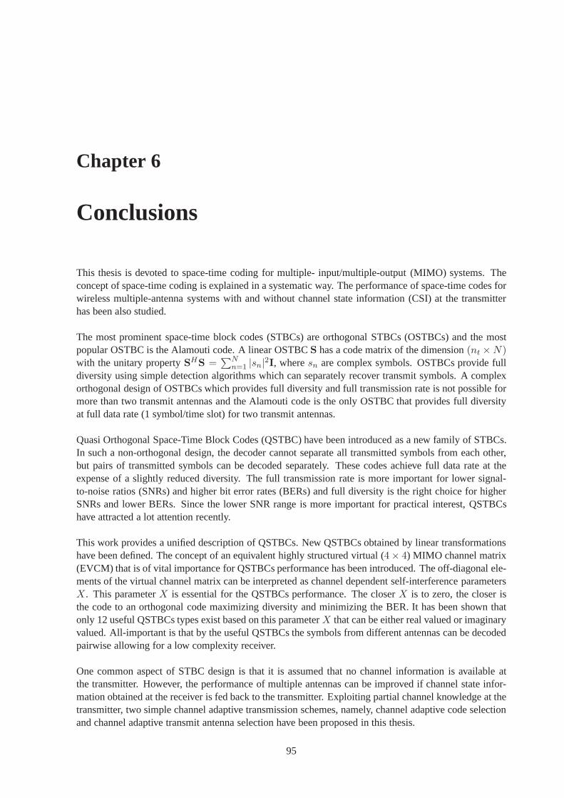
Chapter 6
Conclusions
This thesis is devoted to space-time coding for multiple- input/multiple-output (MIMO) systems. Theconcept of space-time coding is explained in a systematic way. The performance of space-time codes forwireless multiple-antenna systems with and without channel state information (CSI) at the transmitterhas been also studied.
The most prominent space-time block codes (STBCs) are orthogonal STBCs (OSTBCs) and the mostpopular OSTBC is the Alamouti code. A linear OSTBCS has a code matrix of the dimension(nt × N)with the unitary propertySHS =
∑Nn=1 |sn|2I, wheresn are complex symbols. OSTBCs provide full
diversity using simple detection algorithms which can separately recover transmit symbols. A complexorthogonal design of OSTBCs which provides full diversity and full transmission rate is not possible formore than two transmit antennas and the Alamouti code is the only OSTBC that provides full diversityat full data rate (1 symbol/time slot) for two transmit antennas.
Quasi Orthogonal Space-Time Block Codes (QSTBC) have been introduced as a new family of STBCs.In such a non-orthogonal design, the decoder cannot separate all transmitted symbols from each other,but pairs of transmitted symbols can be decoded separately.These codes achieve full data rate at theexpense of a slightly reduced diversity. The full transmission rate is more important for lower signal-to-noise ratios (SNRs) and higher bit error rates (BERs) andfull diversity is the right choice for higherSNRs and lower BERs. Since the lower SNR range is more important for practical interest, QSTBCshave attracted a lot attention recently.
This work provides a unified description of QSTBCs. New QSTBCs obtained by linear transformationshave been defined. The concept of an equivalent highly structured virtual (4× 4) MIMO channel matrix(EVCM) that is of vital importance for QSTBCs performance has been introduced. The off-diagonal ele-ments of the virtual channel matrix can be interpreted as channel dependent self-interference parametersX. This parameterX is essential for the QSTBCs performance. The closerX is to zero, the closer isthe code to an orthogonal code maximizing diversity and minimizing the BER. It has been shown thatonly 12 useful QSTBCs types exist based on this parameterX that can be either real valued or imaginaryvalued. All-important is that by the useful QSTBCs the symbols from different antennas can be decodedpairwise allowing for a low complexity receiver.
One common aspect of STBC design is that it is assumed that no channel information is available atthe transmitter. However, the performance of multiple antennas can be improved if channel state infor-mation obtained at the receiver is fed back to the transmitter. Exploiting partial channel knowledge at thetransmitter, two simple channel adaptive transmission schemes, namely, channel adaptive code selectionand channel adaptive transmit antenna selection have been proposed in this thesis.
95
96
In case of code selection, the receiver returns one or two feedback bits per fading block and (depend-ing on the number of returned bits) the transmitter switchesbetween two or four predefined QSTBCsto minimize the channel dependent self- interference parameterX. In this way full diversity and nearlyfull-orthogonality can be achieved with an ML receiver as well as with a simple ZF receiver. This methodcan be applied to any number of transmit antennas without increasing the required number of feedbackbits.QSTBCs with antenna selection are analyzed based on different selection criterions. The ” best”nt out ofNt transmit antennas are selected for the transmission with respect to a certain selection criterion. Withan optimum selection criterion the same diversity can be achieved as with the system that makes use of allNt transmit antennas. Transmit antenna selection reduces thehardware complexity and achieves the sys-tem diversity as the complete systems were used. With transmit antenna selection, high channel capacitycan be achieved. However, a one drawback of this method is that the number of required feedback bits
increases exponentially with the number of antennas andbfeedback =⌈
log2(qeff)⌉
=⌈
log2
[
(Nt
4
)
] ⌉
bits
have to be returned to inform the transmitter which transmitantenna subset should be used.
In this work new useful QSTBCs have been proposed which can bea good candidate for future wirelesscommunication systems. These useful QSTBCs provide high transmission rate with simple decodingalgorithms and perform very well on i.i.d. MIMO channels as well on realistic MIMO channels. Thedrawback of these codes, a diversity loss, can be avoided by simple closed-loop transmission schemeswhich only require a small amount of feedback bits. Partial channel knowledge at the transmitter in-creases the diversity of QSTBCs and orthogonalizes the QSTBCs opening the way to simple decodingalgorithms that offer a good trade-off between performanceand complexity. Furthermore, QSTBCs us-ing partial channel information make a MIMO system more robust against the negative influences of thewireless channel environment, e.g. high antenna correlations.

Appendices
97
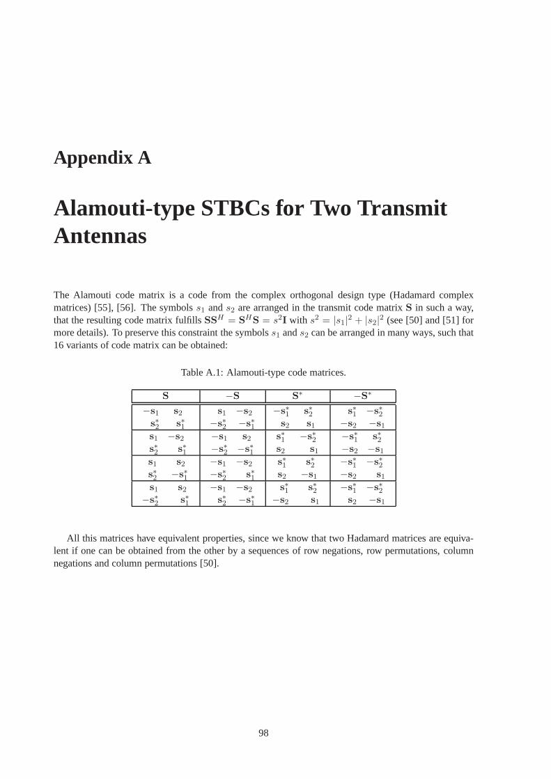
Appendix A
Alamouti-type STBCs for Two TransmitAntennas
The Alamouti code matrix is a code from the complex orthogonal design type (Hadamard complexmatrices) [55], [56]. The symbolss1 ands2 are arranged in the transmit code matrixS in such a way,that the resulting code matrix fulfillsSSH = SHS = s2I with s2 = |s1|2 + |s2|2 (see [50] and [51] formore details). To preserve this constraint the symbolss1 ands2 can be arranged in many ways, such that16 variants of code matrix can be obtained:
Table A.1: Alamouti-type code matrices.
S −S S∗ −S∗
−s1 s2
s∗2 s∗1
s1 −s2
−s∗2 −s∗1
−s∗1 s∗2s2 s1
s∗1 −s∗2−s2 −s1
s1 −s2
s∗2 s∗1
−s1 s2
−s∗2 −s∗1
s∗1 −s∗2s2 s1
−s∗1 s∗2−s2 −s1
s1 s2
s∗2 −s∗1
−s1 −s2
−s∗2 s∗1
s∗1 s∗2s2 −s1
−s∗1 −s∗2−s2 s1
s1 s2
−s∗2 s∗1
−s1 −s2
s∗2 −s∗1
s∗1 s∗2−s2 s1
−s∗1 −s∗2s2 −s1
All this matrices have equivalent properties, since we knowthat two Hadamard matrices are equiva-lent if one can be obtained from the other by a sequences of rownegations, row permutations, columnnegations and column permutations [50].
98
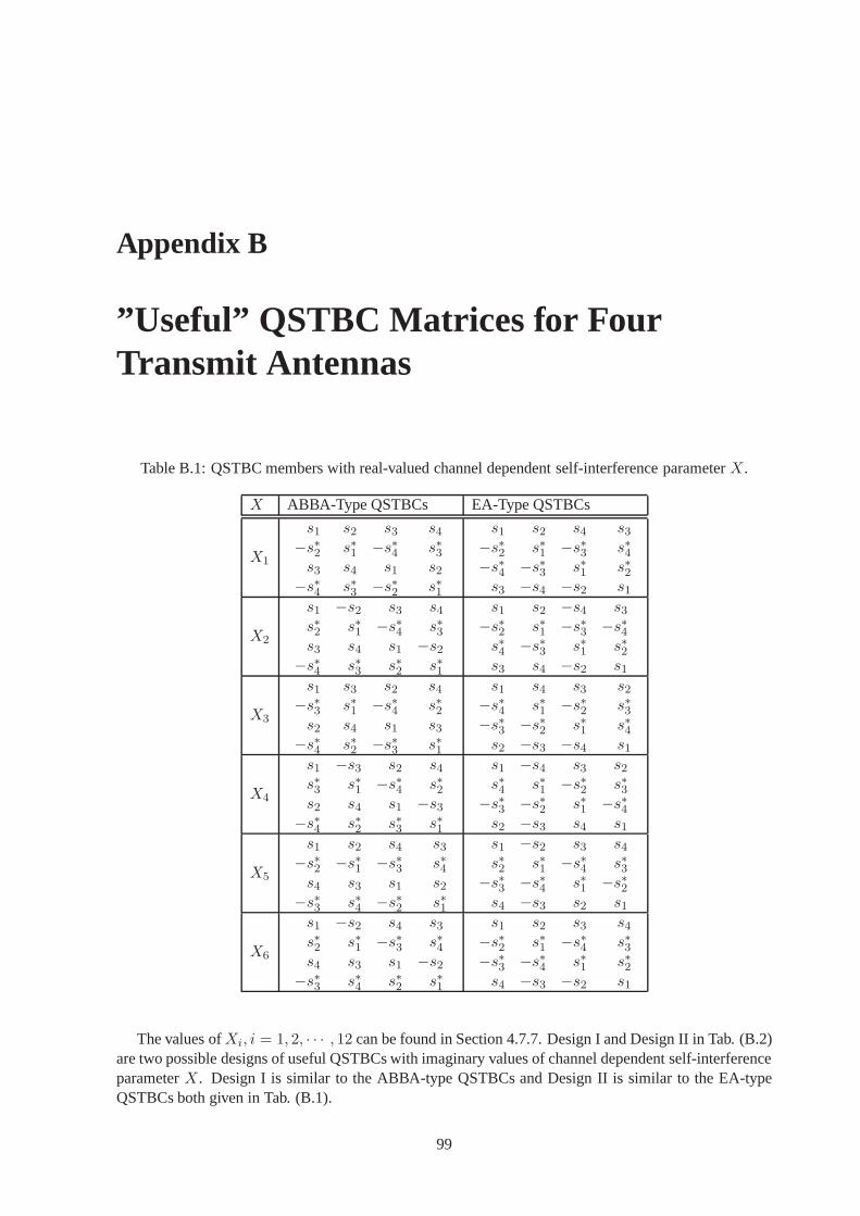
Appendix B
”Useful” QSTBC Matrices for FourTransmit Antennas
Table B.1: QSTBC members with real-valued channel dependent self-interference parameterX.
X ABBA-Type QSTBCs EA-Type QSTBCs
X1
s1 s2 s3 s4
−s∗2 s∗1 −s∗4 s∗3s3 s4 s1 s2
−s∗4 s∗3 −s∗2 s∗1
s1 s2 s4 s3
−s∗2 s∗1 −s∗3 s∗4−s∗4 −s∗3 s∗1 s∗2
s3 −s4 −s2 s1
X2
s1 −s2 s3 s4
s∗2 s∗1 −s∗4 s∗3s3 s4 s1 −s2
−s∗4 s∗3 s∗2 s∗1
s1 s2 −s4 s3
−s∗2 s∗1 −s∗3 −s∗4s∗4 −s∗3 s∗1 s∗2s3 s4 −s2 s1
X3
s1 s3 s2 s4
−s∗3 s∗1 −s∗4 s∗2s2 s4 s1 s3
−s∗4 s∗2 −s∗3 s∗1
s1 s4 s3 s2
−s∗4 s∗1 −s∗2 s∗3−s∗3 −s∗2 s∗1 s∗4
s2 −s3 −s4 s1
X4
s1 −s3 s2 s4
s∗3 s∗1 −s∗4 s∗2s2 s4 s1 −s3
−s∗4 s∗2 s∗3 s∗1
s1 −s4 s3 s2
s∗4 s∗1 −s∗2 s∗3−s∗3 −s∗2 s∗1 −s∗4
s2 −s3 s4 s1
X5
s1 s2 s4 s3
−s∗2 −s∗1 −s∗3 s∗4s4 s3 s1 s2
−s∗3 s∗4 −s∗2 s∗1
s1 −s2 s3 s4
s∗2 s∗1 −s∗4 s∗3−s∗3 −s∗4 s∗1 −s∗2
s4 −s3 s2 s1
X6
s1 −s2 s4 s3
s∗2 s∗1 −s∗3 s∗4s4 s3 s1 −s2
−s∗3 s∗4 s∗2 s∗1
s1 s2 s3 s4
−s∗2 s∗1 −s∗4 s∗3−s∗3 −s∗4 s∗1 s∗2
s4 −s3 −s2 s1
The values ofXi, i = 1, 2, · · · , 12 can be found in Section 4.7.7. Design I and Design II in Tab. (B.2)are two possible designs of useful QSTBCs with imaginary values of channel dependent self-interferenceparameterX. Design I is similar to the ABBA-type QSTBCs and Design II is similar to the EA-typeQSTBCs both given in Tab. (B.1).
99
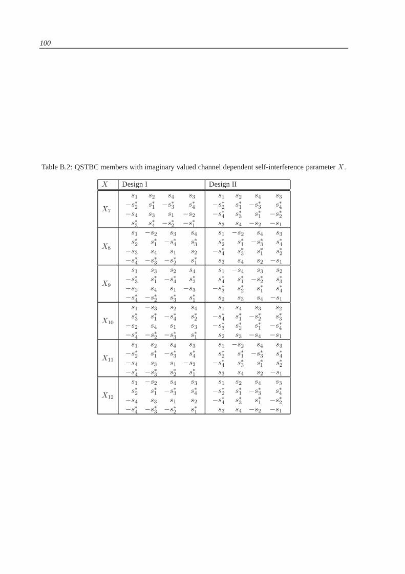
100
Table B.2: QSTBC members with imaginary valued channel dependent self-interference parameterX.
X Design I Design II
X7
s1 s2 s4 s3
−s∗2 s∗1 −s∗3 s∗4−s4 s3 s1 −s2
s∗3 s∗4 −s∗2 −s∗1
s1 s2 s4 s3
−s∗2 s∗1 −s∗3 s∗4−s∗4 s∗3 s∗1 −s∗2
s3 s4 −s2 −s1
X8
s1 −s2 s3 s4
s∗2 s∗1 −s∗4 s∗3−s3 s4 s1 s2
−s∗4 −s∗3 −s∗2 s∗1
s1 −s2 s4 s3
s∗2 s∗1 −s∗3 s∗4−s∗4 s∗3 s∗1 s∗2
s3 s4 s2 −s1
X9
s1 s3 s2 s4
−s∗3 s∗1 −s∗4 s∗2−s2 s4 s1 −s3
−s∗4 −s∗2 s∗3 s∗1
s1 −s4 s3 s2
s∗4 s∗1 −s∗2 s∗3−s∗3 s∗2 s∗1 s∗4
s2 s3 s4 −s1
X10
s1 −s3 s2 s4
s∗3 s∗1 −s∗4 s∗2−s2 s4 s1 s3
−s∗4 −s∗2 −s∗3 s∗1
s1 s4 s3 s2
−s∗4 s∗1 −s∗2 s∗3−s∗3 s∗2 s∗1 −s∗4
s2 s3 −s4 −s1
X11
s1 s2 s4 s3
−s∗2 s∗1 −s∗3 s∗4−s4 s3 s1 −s2
−s∗4 −s∗3 s∗2 s∗1
s1 −s2 s4 s3
s∗2 s∗1 −s∗3 s∗4−s∗4 s∗3 s∗1 s∗2
s3 s4 s2 −s1
X12
s1 −s2 s4 s3
s∗2 s∗1 −s∗3 s∗4−s4 s3 s1 s2
−s∗4 −s∗3 −s∗2 s∗1
s1 s2 s4 s3
−s∗2 s∗1 −s∗3 s∗4−s∗4 s∗3 s∗1 −s∗2
s3 s4 −s2 −s1
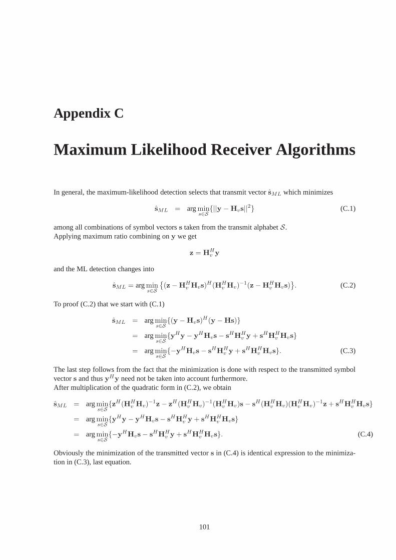
Appendix C
Maximum Likelihood Receiver Algorithms
In general, the maximum-likelihood detection selects thattransmit vectorsML which minimizes
sML = argmins∈S
{||y − Hvs||2} (C.1)
among all combinations of symbol vectorss taken from the transmit alphabetS.Applying maximum ratio combining ony we get
z = HHv y
and the ML detection changes into
sML = argmins∈S
{
(z −HHv Hvs)
H(HHv Hv)
−1(z − HHv Hvs)
}
. (C.2)
To proof (C.2) that we start with (C.1)
sML = argmins∈S
{(y − Hvs)H(y − Hs)}
= argmins∈S
{yHy − yHHvs − sHHHv y + sHHH
v Hvs}
= argmins∈S
{−yHHvs − sHHHv y + sHHH
v Hvs}. (C.3)
The last step follows from the fact that the minimization is done with respect to the transmitted symbolvectors and thusyHy need not be taken into account furthermore.After multiplication of the quadratic form in (C.2), we obtain
sML = argmins∈S
{zH(HHv Hv)
−1z − zH(HHv Hv)
−1(HHv Hv)s − sH(HH
v Hv)(HHv Hv)
−1z + sHHHv Hvs}
= argmins∈S
{yHy − yHHvs− sHHHv y + sHHH
v Hvs}
= argmins∈S
{−yHHvs− sHHHv y + sHHH
v Hvs}. (C.4)
Obviously the minimization of the transmitted vectors in (C.4) is identical expression to the minimiza-tion in (C.3), last equation.
101
Appendix D
Acronyms
AWGN Additive WhiteGaussianNoiseBER Bit Error RatioBLAST Bell Labs-LayeredSpace-TimeCAAS ChannelAdaptiveAntennaSelectionCACS ChannelAdaptiveCodeSelectionCSI ChannelStateInformationEA ExtendedAlamoutiEVCM EquivalentVirtual ChannelMatrixi.i.d independentlyidenticaldistributedMIMO Multiple InputMultiple OutputMISO Multiple InputSingle OutputML MaximumLikelihoodMMSE Minimum MeanSquareErrorMRC MaximumRatio CombiningOSTBC OrthogonalSpace-Time Block-CodePEP PairwiseError ProbabiltyPDF ProbabiltyDensityFunktionQPSK QuadraturePhaseShift KeyingQSTBC Quasi-OrthogonalSpace-Time Block CodesSER Symbol Error RatioSISO Single InputSingle OutputSIMO Single InputMultiple OutputSM SpatialMultiplexingSTBC Space-Time Block CodeSNR Signal toNoiseRatioSTC Space-Time CodingSTTC Space-Time Trellis CodeULA Uniform LinearArrayZF ZeroForcing
102
Bibliography
[1] I.E.Telatar, “Capacity of Multi-Antenna Gaussian Channels”, AT&T Bell Labs,http://mars.belllabs.com/cm/ms/what/mars/papers/proof, 1995.
[2] G. J. Foschini, M. J. Gans, “On Limits of Wireless Communications in Fading Environments whenUsing Multiple Antennas”, Wireless Personal Communications, vol. 6, pp. 311-335, March 1998.
[3] V. Tarokh, N. Seshadri, A. R. Calderbank, “Space-Time Codes for High Data Rate Wireless Com-munication: Performance Criterion and Code Construction”, IEEE Trans. Inform. Theory, vol. 44,no. 2, pp. 744-765, March 1998.
[4] Z. Liu, G. B. Giannakis, S. Zhou, B. Muquet, ”Space-time coding for boradband wireless commu-nications”, Wireless Communications and Moblie Computing, vol. 1, no. 1. pp. 35-53, Jan. 2001.
[5] J. H. Winters, ”On the capacity of radio communication systems with diversity in a Rayleigh fadingenvironment”, IEEE Journal on Selected Areas in Communications, pp. 871-878, June 1987.
[6] A. Wittneben, ”A new bandwidth efficient transmit antenna modulation diversity scheme for lineardigital modulation”, IEEE Int. Conference on Com., vol. 3, pp. 1630 - 1634, Geneva, May 1993.
[7] V. Tarokh, N. Seshadri, A. R. Calderbank, “Combined Array Processing and Space-Time Coding”,IEEE Trans. Inform. Theory, vol. 45, no. 5, pp. 1121 - 1128, May 1999.
[8] A. Hottinen, O. Tirkkonen, R. Wichman,”Multi-Antenna Transceiver Techniques for 3G and Be-yond”, John Wiley and Son Ltd. 2003.
[9] M. K. Simon, M.-S. Alouini,Digital Communication over Fading Channel: A Unified Approach toPerformance Analysis, John Wiley& Sohn, 2000.
[10] T. S. Rappapot,Wireless Communications: Principles and Practice, Prentice Hall, 1996.
[11] M. Rupp, H. Weinrichter, G. Gritsch, ”Approximate ML Detection for MIMO Systems with VeryLow Complexity”, ICASSPO04, Montreal, Canada, pp. 809-812, May 2004.
[12] H. Artes, D. Seethaler, F. Hlawatsch, ”Efficient Detection Algorithms for MIMO Channels: Ageometrical Approach to Approximate ML Detection”, IEEE Transactions on Signal Processing,Special Issue on MIMO communications Systems, vol. 51, no. 11, pp. 2808-2820, Nov. 2003.
[13] U. Fincke, M. Phost, ”Improved methods for calculatingvectors of short length in a lattice, includ-ing a complexity analysis”, Math. of Comp., vol. 44, pp. 463-471, April 1985.
[14] S. Verdu,”Multiuser Detection”, Cambridge University Press, New York, 1998.
[15] John G. Proakis,”Digital Communications”, 3rd ed. McGraw-Hill, Inc. 1995.
103
104 BIBLIOGRAPHY
[16] M. Herdin, “Non-Stationary Indoor MIMO Radio Channels”, Ph.D. Thesis, Vienna University ofTechnology, Aug. 2004.
[17] J. Fuhl, A. F. Molisch, E. Bonek, “Unified Channel Model for Mobile Radio Systems with SmartAntennas”, IEE Proceedings Pt. F. (Radar, Sonar and Navigation), vol. 145, no. 1, pp. 32-41, Feb.1998.
[18] M. T. Ivrlac, T. P. Kurpjuhn, C. Brunner, W. Utschick, “Efficient use of fading correlation in MIMOsystems”, 54th VTC, Atlantic City, USA, vol. 4, pp. 2763-2767, Oct. 2001.
[19] J. P. Kermoal, L. Schumacher, K. I. Pedersen, P. E. Mogensen, F. Frederiksen, “A Stochastic MIMORadio Channel Model With Experimental Validation”, IEEE Journal on Selected Areas in Commu-nications, vol. 20, no. 6, pp. 1211-1226, Aug. 2002.
[20] W. Weichselberger, M. Herdin, H.Ozcelik, E. Bonek, “A Novel Stochastic MIMO Channel Modeland its Physical Interpretation”, International Symposium on Wireless Personal Multimedia Com-munications, Yokosuka, Japan, 19. - 22. Oct. 2003.
[21] Da-Shan Shiu, G. J. Foschini, M. J. Gans, J. M. Kahn, “Fading Correlation and Its Effect on theCapacity of Multielement Antenna Systems”, IEEE Transactions on Communications, vol. 48, no.3, pp. 502-513, March 2000.
[22] Chen-Nee Chuah, J. M. Kahn, D. Tse, “Capacity of Multi-Antenna Array Systems in Indoor Wire-less Environment”, Globecom, Sydney, Australia, vol. 4, pp. 1894-1899, Nov. 998.
[23] W. Weichselberger, “Spatial Structure of Multiple Antenna Radio Channels - A Signal ProcessorViewpoint”, Ph.D. Thesis, Vienna University of Technology, Dec. 2003.
[24] H. Ozcelik, M. Herdin, W. Weichselberger, J. Wallace, E.Bonek,“Deficiencies of the KroneckerMIMO radio channel model”, Electronics Letters, vol. 39, pp. 1209-1210, Aug. 2003.
[25] K. I. Pedersen, J. B. Andersen, J. P. Kermoal, P. Mogenesen, ”A Stochastic Multiple-Input-Multiple-Output Radio Channel Model for Evaluation of Space-Time Coding Algorithms”, 52ndVTC, vol. 2, pp. 893-897, Sept. 2000.
[26] C. E. Shannon, ” A mathematical theory of communication”, Bell Syst. Tech. J.,vol. 27, pp. 379-423, Oct. 1948.
[27] B. Vucetic, J. Yuan,”Space-Time Coding”, John Wiley & Sons, England, 2003.
[28] R. A. Horn, C. R. Johnson,Matrix Analysis, New York, Cambridge Univ. Press. 1988.
[29] S. Alamouti, “A Simple Transmitter Diversity Technique for Wireless Communications”, IEEEJournal on Selected Areas of Communications, Special Issueon Signal Processing for WirelessCommunications, vol.16, no.8, pp.1451-1458, Oct. 1998.
[30] V. Tarokh, N. Seshadri, A.R. Calderbank, “Space-time codes for high data rate wireless communi-cation: Performance criterion and code construction,” IEEE Trans. Inform. Theory, vol. 44, no. 2,pp. 744–765, March 1998.
[31] V. Tarokh, H. Jafarkhani, A.R. Calderbank, ”Space-time block coding for wireless communications:Performance results,” IEEE Journal on Sel. Areas in Com., vol.17, no. 3, pp. 451-460, Mar. 1999.
[32] V. Tarokh, H. Jafarkhani and A. R. Calderbank, ”Space-time block codes from orthogonal designs,”IEEE Trans. Inform. Theory, vol. 45, pp. 1456-1467, July 1999.
BIBLIOGRAPHY 105
[33] O. Tirkkonen, A. Hottinen, ”Complex Space-Time Block Codes for four TX antennas”, Globecom2000, vol. 2, pp. 1005-1009, Dec. 2000.
[34] M. Rupp, C. F. Mecklenbrauker, “On Extended Alamouti Schemes for Space-Time Coding”,WPMC, Honolulu, pp. 115-118, Oct. 2002.
[35] H. Jafarkhani and N. Seshadri, Super-orthogonal space-time trellis codes, IEEE Trans. Inform.Theory, vol. 49, pp. 937-950, Apr. 2003.
[36] Z. Chen, J. Yuan, B. Vucetic, “An improved space time trellis coded modulation scheme on slowRayleigh fading channels”, IEE Electronics Letters., vol.37, no. 7, pp. 440-441, Mar. 2001.
[37] Z. Chen, B. Vucetic, J. Yuan, K. L. Lo, “Space-time trellis codes with two three and four transmitantennas in quasi-static flat channels”, IEEE Communication Letter, vol. 6, no. 2, Feb. 2002.
[38] B. Vucetic, J. Nicolas, ”Performance of 8PSK trellis codes over nonlinear fading mobile satellitechannels”, Inst. Elect. Eng. Proc. I, vol. 139, pp. 462-471,Aug. 1992.
[39] A. Papoulis,Probability, Random Variables and Stochastic Processes,McGraw-Hill, 4.Ed., 2002.
[40] G. Ganesan, P. Stoica, ”Space-time diversity using orthogonal and amicable orthogonal design”,Wireless Personal Communications, vol. 18, pp. 165-178, 2001.
[41] E. G. Larsson, P. Stoica,”Space-Time Block Coding for Wireless Communications”, CambridgeUniversity Press, Cambridge UK, 2003.
[42] H. Jafarkhani, ”A quasi orthogonal space-time block code,” IEEE Trans. Comm., vol. 49, pp. 1-4,Jan. 2001.
[43] O. Tirkkonen, A. Boariu, A. Hottinen, ”Minimal nonorthogonality rate one space-time block codesfor 3+ Tx antennas,” IEE International Symposium on Spread Spectrum Techniques and Applica-tions (ISSSTA), vol. 2, New Jersey, USA, pp. 429-432, Sept. 2000.
[44] C. Papadias, G. Foschini, ”Capacity-Approaching Space-Time Codes for System Employing FourTransmitter Antennas”, IEEE Trans. Inf. Theory, vol. 49, no. 3, pp. 726-733, March 2003.
[45] C.F. Mecklenbrauker, M. Rupp, ”On extended Alamouti schemes for space-time coding,”,WPMC’02, Honolulu, pp. 115-119, Oct. 2002.
[46] F. C. Zheng, A. G. Burr, ”Robust non-orthogonal space-time block codes over highly correlatedchannels: a generalisation, ”IEE El. Letters, vol. 39, no. 16, pp. 1190-1191, Aug. 2003.
[47] C.F. Mecklenbrauker, M. Rupp, ”Flexible space-time block codes for trading quality of serviceagainst data rate in MIMO UMTS,” EURASIP J. on Appl. Signal Proc., no. 5, pp. 662-675, May2004.
[48] J. Hou, M.H. Lee, J.Y. Park, ”Matrices analysis of quasi-orthogonal space-time block code,” IEEECommunications Letters, vol. 7, no. 8, pp. 385-387, Aug. 2003.
[49] C. Yuen, Y. L. Guan, T. T. Tjhung, ”Decoding of Quasi-Orthogonal Space-Time Block Code withNoise Whitening”, 14th IEEE international Symposium on Personal, Indoor and Mobile RadioCommunication Proceedings, Beijing, China, pp. 2166-2170, Sept. 2003
[50] R.J. Turyn,Complex Hadamard Matrices, Structure und their Applications, Gordon and Breach,New York, 1970.
106 BIBLIOGRAPHY
[51] S. Rahardja, B.J. Falkowski, ”Family of complex Hadamard transforms: relationship with othertransforms and complex composite spectra”, 27th International Symposium on Multiple-ValuedLogic, pp. 125-130, May 1997.
[52] M. Rupp , C.F. Mecklenbrauker, G. Gritsch, ”High Diversity with Simple Space Time Block-Codes”, Proc. of Globecom 03, vol. 1, pp.302-306, San Francisco, USA, 2003.
[53] M. Rupp, H. Weinrichter, G. Gritsch, “Approximate ML Detection for MIMO Systems with VeryLow Complexity”, ICASSP’04, Montreal, Canada, pp. 809-812, May 2004.
[54] Gerhard Gritsch , Error Performance of Multiple Antenna Systems, Dissertation, TU Wien (2004).
[55] J. Seberry, M. Yamada ”Hadamard matrices, sequences and block designs”,Contemporary DesignTheory: A Collection of Surveys, eds., J. Dinitz, D. Stinson, J. Wiley, New York, pp. 431-560, 1992.
[56] J. Seberry, R. Craigen. ”Orthogonal Designs”, inHandbook of Combinatorial Designs, C.J. Col-bourn, J.H. Dinitz, CRC Press, pp. 400-406, 1996.
[57] H. Ozcelik, M. Herdin, H. Hofstetter, E. Bonek, ”A comparsion of measured8× 8 ”MIMO systemwith a popular stochastic channel model at 5.2 GHz,” 10th International Conference on Telecom-munications (ICT’2003), Tahiti, March 2003.
[58] H. Ozcelik, M. Herdin, R. Prestros, E. Bonek, ”How MIMO capacity is linked with single elementfading statistics”, International Conference on Elektromagnetics in Advanced Applications, Torino,Italy, pp. 775-778, Sept. 2003.
[59] R.S. Thoma, D. Hampicke, A. Richter, G. Sommerkorn, A.Schneider, U.Trautwein, W.Wirnitzer,”Identification of time-variant directional mobile radio channels”, IEEE Transactions on Instru-mentation and Measurement, vol.49, pp.357-364, April 2000.
[60] B. Badic, M. Herdin, G. Gritsch, M. Rupp, H. Weinrichter”Performance of various data transmis-sion methods on measured MIMO channels,” 59th IEEE Vehicular Technology Conference VTCSpring 2004, Milan, Italy, May 2004.
[61] B. Badic, M. Herdin, M. Rupp, H. Weinrichter, ”Quasi Orthogonal Space-Time Block Codes onMeasured MIMO Channels,” SympoTIC 04, Bratislava, pp. 17-20, Oct. 2004.
[62] S. Zhou, Z. Wang, G.B. Giannakis, ”Performance analysis for transmit-beamforming with finite-rate feedback,” Proc. of Conference on Information Sciences and Systems, Princeton University,Princeton, NJ, March 2004.
[63] K. Mukkavilli, A. Sabharwal, E. Erkip, B. Aazhang, ”On beamforming with finite rate feedback inmultiple antenna systems,” IEEE Transactions on Information Theory, vol. 49, No. 10, pp. 2562-2579, Oct. 2003.
[64] J. Akhtar, D. Gesbert, ”Partial feedback based orthogonal block coding,” Proc. of the 57th IEEESemiannual Vehicular Technology Conference, 2003, VTC 2003-Spring, vol.1, pp. 287-291, April2003.
[65] B. Badic, M. Rupp, H. Weinrichter, ”Adaptive channel matched extended Alamouti space-timecode exploiting partial feedback,” Proc. of the International Conference on Cellular and IntelligentCommunications (CIC), Seoul, Korea, pp. 350-354, Oct. 2003.
[66] B. Badic, M. Rupp, H. Weinrichter, ”Extended alamouti codes in correlated channels using partialfeedback”, IEEE International Conference on Communications, vol. 2, pp. 896 - 900, Paris, France,June 2004
BIBLIOGRAPHY 107
[67] B. Badic, H. Weinrichter, M. Rupp, ”Comparison of Non-Orthogonal Space-Time Block Codes inCorrelated Channels,” SPAWC 04, Lisboa, July 2004.
[68] G. Jongren, M. Skoglund, ”Utilizing quantized feedback information in orthogonal space-timeblock coding,” Proc. of Glob. Telecom. Conference, vol. 2, pp. 1147-1151, Nov. 2002.
[69] E.G. Larsson, G. Ganesan, P. Stoica, W.H. Wong, ”On the performance of orthogonal space-timeblock coding with quantized feedback,” IEEE Com. Letters, vol. 6, pp. 487-489, Nov. 2002.
[70] K. K. Mukkavilli, A. Sabharwal, B. Aazhang, ”Design of Multiple Antenna Coding Schemes withChannel Feedback”, Asilomar Conference on Signals, Systems, and Computers, Pacific Grove, CA,pp. 1009-1013, Nov. 2001.
[71] D. Love, R. Heath, ”Diversity performance of precoded orthogonal space-time block codes usinglimited feedback,” IEEE Communications Letters, vol.8, pp. 308-310, May 2004.
[72] S. Caban, C. Mehlfuhrer, R. Langwieser, A. L. Scholtz,M. Rupp, ”MATLAB Interfaced MIMOTestbed,” , in press EURASIP Journal on Applied Signal Processing, 2005.
[73] C. Mehlfuhrer, S. Geirhofer, S. Caban, M. Rupp ”A Flexible MIMO Testbed with Remote Access”,13th European Signal Processing Conference (EUSIPCO 2005), Antalya, Turkey, Sep. 2005.
[74] D.A. Gore, R.U. Nabar, A. Paulraj, “Selecting an Optimal Set of Transmit Antennas for a Low RankMatrix Channel,” ;IEEE International Conference on Acoustics, Speech, and Signal Processing,2000. ICASSP ’00, vol. 5, pp. 2785 - 2788, June 2000.
[75] S. Sandhu, R.U. Nabar, D.A. Gore, A. Paulraj, “Near-Optimal Selection of Transmit Antennas fora MIMO Channel Based on Shannon Capacity,”Conference Record of the Thirty-Fourth AsilomarConference on Signals, Systems and Computers, 2000, vol. 1, pp. 567 - 571, Oct. 2000.
[76] R.W. Heath Jr., S. Sandhu and A. Paulraj, “Antenna Selection for Spatial Multiplexing Systemswith Linear Receivers,”IEEE Communications Letters, vol. 5, is. 4, pp. 142 - 144, April 2001
[77] D. Gore, A. Paulraj, ”Space-time block coding with optimal antenna selction,” IEEE InternationalConference on Acoustics, Speech, Signal Processing, vol 4,pp. 2441-2444, May 2001.
[78] Z. Chen, J. Yuan, B. Vucetic, Z. Zhou, ”Performance of Alamouti scheme with transmit antennaselection,’ IEEE Electronic Letters, vol. 39, no. 23, pp. 1666-1668, Nov. 2003.
[79] A.F. Molisch, M.Z. Win, ”MIMO Systems with Antenna Selection”, IEEE Microwave Magazine,vol.5, pp. 46-56, March 2004.
[80] B. Badic, P. Fuxjager, H. Weinrichter, ”Performance of a Quasi-Orthogonal Space-Time Code withAntenna Selection”, IEE El. Letters, vol. 40, no. 20, pp. 1282-1284, Sep. 2004.
[81] B. Badic, P. Fuxjager, H. Weinrichter , ”Optimizationof Coded MIMO-Transmission with AntennaSelection,” Proc. 2005 IEEE 61 st Vehicular Technology Conference, VTC2005 - Spring, 30 May-1 June 2005, Stockholm Sweden.
[82] S. Barbarossa,”Multiantenna Wireless Communication Systems”, Artech House, INC, 2005.
[83] S. S. Paulraj, ”Space-Time Block Codes: a capacity perspective”, IEEE Communications Letters,vol. 4, pp. 384-386, Dec. 2000.
[84] C. Papadias, G. Foschini, ”Capacity Approaching Space-Time Codes for Systems Employing FourTransmit Antennas”, IEEE Transaction on Information Theory, vol. 49, no.3, pp. 726-733, March2003.