Space Object Data Association Using Spatial Pattern Recognition...

Space Object Data Association

Using Spatial Pattern Recognition Approaches

Aniketh Kalur∗

University of Minnesota, Minneapolis, MN 55455

Steven A. Szklany† and John L. Crassidis‡

University at Buffalo, State University of New York, Amherst, NY 14260-4400

Closely-spaced objects, especially debris objects, create a setting that is very similar to amulti-target environment in a tracking problem. This environment engenders a major dataassociation problem in the field of space situational awareness. To address this problem,an approach that couples gating methods for data association along with a star patternrecognition algorithm, called the planar triangular method, is developed. The planar tri-angular method has been shown to work effectively for spacecraft attitude determinationusing star trackers by comparing stars in field-of-view to those present in the catalog. Thisapproach is further enhanced here for association of resident space objects. The planartriangle approach is further enhanced to associate closely spaced objects by incorporatinga classical validation gate-based algorithm. The work in this paper shows the effectivenessof combining traditional data association methods with an existing planar triangle patternrecognition algorithm for space object association. Results indicate that the traditionalgating algorithm significantly improves the planar triangular method’s accuracy for spaceobject association of closely-spaced clutters in highly uncertain environments.

I. Introduction

Space Situational Awareness (SSA) deals with collecting and maintaining knowledge of all objects orbitingthe Earth. It is defined as the comprehensive knowledge of space objects and the ability to track, understandand predict their future location. The orbits in space are comprised of functional and defunct objects, aswell as artificial objects. Functional objects are actively controlled so that their attitude and position can bemaintained to accomplish mission objectives. However, defunct objects generally are not actively controlledfor attitude and positional corrections. Inability to control objects in space renders them as “space junk;”these objects are rarely of any use and cause a threat to functional objects that are currently in orbit.Defunct objects are often spent rocket stages, inoperable satellites or parts of spacecraft that were oncefunctional. Most uncontrolled objects are often referred to as orbital debris. Generally these objects do notfollow pure Keplerian motion, being subjected to drift and decay. For example, variations in the Earth’sgravitational field cause drift, which can lead to gradual movement of an object from one orbital plane toanother. Atmospheric drag is a major cause of orbital decay, thereby causing a slow decrease in altitude ofthe object. Solar radiation pressure can also affect an object’s orbit. Taken together, uncontrolled objectspose a difficult problem in maintaining adequate SSA.

A very common term associated with Resident Space Objects (RSOs) in space is Kessler’s syndrome,which theorizes that creation of new debris occurs faster than the time taken by natural forces to removethem. As space object density increases, the collision between objects could cause a cascading effect, i.e. eachcollision generates more debris and thereby increases the likelihood of further collisions. There are more than

∗Graduate Student, Department of Aerospace Engineering & Mechanics. Email: [email protected].†Graduate Student, Department of Mechanical & Aerospace Engineering. Email: [email protected].‡CUBRC Professor in Space Situational Awareness, Department of Mechanical & Aerospace Engineering. Email:

[email protected]. Fellow AIAA.

1 of 21

American Institute of Aeronautics and Astronautics

21,000 piece of debris with a radius larger than 10 centimeters. These 21,000 pieces of debris are open tothe same threat of collisions as defined by the Kessler’s syndrome. A recent consequence of these debrisobjects is the International Space Station (ISS), which had to perform five collision avoidance maneuvers in2014. This has been the highest number of avoidance maneuvers recorded since 1998.1 On July 16, 2015 theISS crew were forced to scramble to safety in the Soyuz escape capsule after NASA received data on a fastapproaching space debris object. The data regarding the debris being in close proximity, and on a highlyprobable collision course with the ISS, was received late and was imprecise as well. Hence the ISS could notmake any evasive maneuvers. Close collision encounters not only endanger humans lives but pose a majorthreat to the many functional spacecraft and scientific equipment present in space. This makes it imperativeto effectively study and develop methods for information fusion and RSO association to improve SSA.

The primary step in resolving the ever growing issue of space debris is proper association and identificationof RSOs. Typically, RSOs are identified by matching sensor measurements (e.g. space-surveillance telescopedata) to a space object catalog of previously identified objects. If the current RSO cannot be matched withany cataloged object, then that object is deemed an unidentified object, otherwise known as an “uncorrelatedtrack,” which is placed in the catalog and monitored throughout its entire life span if possible. Note that someagencies require that the object be determined all the way back to its launch origin to be identified. A catalogis simply a directory of objects that includes information pertaining to the object’s estimated position andcharacteristics, such as the ballistic coefficient-like term found in two-line elements. The process of matchingsensor measurements to a target, or RSO, is known as data association. It is important to note that anassociated object may not be an identified object. Data association is fundamental in determining whichRSOs within a sensor’s field-of-view (FOV) are cataloged, and which are previously unidentified objects. Anaccurate and up-to-date RSO catalog is critical in avoidance maneuver planning and overall SSA.2

Much work has been done in the area of identification and data association in the recent years. Thesecan be broadly divided into Gaussian and non-Gaussian methods. A covariance-based track associationapproach is shown in Ref. 3. An entropy-based data association approach for non-Gaussian probabilitydensity functions (pdfs) is shown in Ref. 4. Tracking multiple number of objects using finite-set statisticsand finite mixture-model representations of multi-object pdfs is developed in Ref. 5. A Gaussian mixtureProbability Hypothesis Density filter for multiple space object tracking is presented in Ref. 6. The ∂-GeneralLabeled Multi-Bernoulli filter has been studied for tracking a large number of objects in Ref. 7. The useof magnetometers in identifying space objects in geosynchronous orbits has been studied and discussed inRef. 8. Each of the aforementioned algorithms has its advantages and disadvantages. For example, Gaussian-based approaches may not work well when the pdf is non-Gaussian, and non-Gaussian approaches may becomputationally expensive and also overburdensome when Gaussian pdfs exist.

The work presented here provides an alternate RSO data association approach, which has its roots instar pattern recognition.9 Pattern recognition is a mature subject in the functionality of star trackers. Astar tracker is an optical device, which collects star measurements in order to determine the attitude of itshost spacecraft. One way stars are identified is by comparing the angles between observed stars in the startracker’s FOV with angles stored in a star catalog. This identification process is known as the angle method.If the angles of the observed stars match the angles of a set of stars in the catalog, then the spacecraft’sattitude can be determined. Given the criticality of attitude knowledge to the performance of a spacecraft,the primary step is to consistently identify stars within the star tracker’s FOV without requiring significantcomputation effort. The additional work on pattern recognition has led to the development of a methodthat uses planar triangle properties for spacecraft attitude determination in lieu of the angle method. Thismethod is called the “Planar Triangle Method” (PTM).10 The PTM is shown to be an accurate and efficientmethod of pattern recognition, and has been proven to work very well for spacecraft attitude determination.Pattern recognition algorithms attempt to match measurements with a certain target by using geometricdata analysis. Given a cluster of data and stored a priori knowledge of the suspected targets, it is anticipatedthat this data will maintain a specific pattern that can be associated with the assigned targets. This workuses the PTM as an effective pattern recognition method for effective RSO data association.

Data association is the process of matching an unknown measured object to its known truth. Problemsattributed to associating the true object from a cluster of similar objects can be addressed by variousmethods. These problems have been very well studied for the case of target tracking and multiple targettracking.11 Data association has been studied in detail for target tracking in surveillance systems employingone or more sensors. In particular, many algorithms such as nearest neighbor, global nearest neighbor,multiple hypothesis tracking, joint probabilistic data association have been extensively studied.11 Coupling

2 of 21


traditional data association techniques with other methods for SSA is the focus of this work. In this papertraditional data association methods, such as elliptical/validation gates, are used to improve the associationof the RSO when combined with the PTM. In traditional star identification algorithms, the errors in thereference vector are orders of magnitude smaller than the focal-plane errors, so that reference errors can beignored in the pattern recognition algorithm. Here, errors in the RSO position significantly contribute tothe overall uncertainty of the observation-to-truth correlation.

The outline of this paper proceeds as follows. First, the dynamics and measurement models are reviewed.Then, the PTM and traditional data association methods are discussed, as well as their combination for theRSO data association problem. Next, simulation results are presented for both uncluttered and clutteredenvironments. Finally, conclusions are drawn upon the simulation results.

II. Dynamics and Measurement Models

This section briefly covers the RSO dynamics model, as well as the focal-plane sensor model used fortelescopes. A derivation of the errors induced on the focal-plane measurements due to RSO estimation errorsis also shown. There are many forces acting on an RSO that perturb it away from the nominal orbit. Theseperturbations, or variations in the orbital elements, can be classified based on how they affect the Keplerianelements. The three basic type of orbital perturbations are secular variations, short period variations andlong period variations. Secular variations have a long term linear variation on the orbit prediction, they causethe orbital elements to increase or decrease as time progresses. The main types of perturbation faced by abody in space are third-body perturbations, atmospheric drag, J2 perturbations, solar radiation pressure,etc. Here, only J2 perturbations are considered. The gravity potential for an arbitrary body is expressedas12

V (r, φ) = −Gmr

[1−

∞∑k=2

(reqr

)kJkPk(sinφ)

](1)

where G is gravitational constant, m is mass of the body, req is the equatorial radius of the body, r is thedistance to a point away from the body, Jk is the kth zonal gravitational harmonic, Pk is the kth orderLegendre polynomial, and φ is the elevation angle of the vector tracking a point away from the body. Theperturbing acceleration due to J2 harmonics is given by

aJ2= −3

2J2

(µg

r2

)(reqr

)2(

1− 5(zr

)2) xr(

1− 5(zr

)2) yr(

3− 5(zr

)2) zr

(2)

The dynamics model for the ith RSO is given by

rRSOi = − µ

r3irRSOi + aJ2i (3)

where µ = Gm, rRSOi = [xi yi zi]

T and ri = ‖rRSOi ‖.

Unit vector observations are assumed here. Focal-plane detectors form measurements according to a setof collinearity equations, which are standard in many photogrammetry applications.13 Assuming that thecamera boresight is aligned with the z-axis, these are given by

αi = −f A11 (xi −X) +A12 (yi − Y ) +A13 (zi − Z)

A31 (xi −X) +A32 (yi − Y ) +A33 (zi − Z), i = 1, 2, . . . , N (4a)

βi = −f A21 (xi −X) +A22 (yi − Y ) +A23 (zi − Z)

A31 (xi −X) +A32 (yi − Y ) +A33 (zi − Z), i = 1, 2, . . . , N (4b)

where f is the focal length, (X, Y Z) is the sensor (instrument) coordinates, denoted in vector form byrINSTR = [X Y Z]T , and Aij are the elements of the attitude matrix, which is a proper orthogonal 3 × 3matrix, denoted by A. This matrix is given by three succussive rotations, given by

A = AT /U AU/F AF/I (5)

3 of 21


where T denotes the Instrument (INSTR) coordinate system, U denotes the local East-North-Up (ENU)coordinate system, F denotes Earth-Centered Earth-Fixed (ECEF) coordinate system, and I Earth-CenteredInertial (ECI) coordinate system. The ENU coordinate system is formed by a plane tangent to Earth’ssurface at a specific location. The origin of the tangent plane is usually dictated by the geolocation of aradar, telescope, or other instrument. Conversions between the various frames can be found in Ref. 14.

The observation vector that is directly measured by the instrument is

γi ≡[αi

βi

](6)

and the corresponding measurement equation with noise is

γi = γi + wi (7)

The zero-mean Gaussian noise process wi is assumed to have covariance given by

RFOCALi =

σ2

1 + d (α2i + β2

i )

[(1 + dα2

i

)2(dαiβi)

2

(dαiβi)2 (

1 + dβ2i

)2]

(8)

where d is on the order of one (and often simply set to one) and σ is assumed to be known.15

In unit vector form, the observations are

bi = Ari, i = 1, 2, . . . , N (9)

where

bi ≡1√

f + α2i + β2

i

−αi

−βif

(10a)

ri ≡1√

(xi −X)2

+ (yi − Y )2

+ (zi − Z)2

xi −Xyi − Yzi − Z

(10b)

The measurement equation for the unit vector is

bi = bi + υi, υTibi = 0 (11)

where the statistics of the noise υi are given by

E{υi} = 0 (12a)

RQUESTi ≡ E

{υiυ

Ti

}= σ2

(I3×3 − bib

Ti

)(12b)

where I3×3 is a 3× 3 identity matrix. The QUEST measurement model16 of Eq. (12b) makes the generallyreasonable assumption that the uncertainty in the line-of-sight (LOS) unit vector measurement lies in thetangent plane to the unit sphere at the point where it intersects the measurement. This assumption becomesless valid for sensors with a wide FOV and LOS vectors far from the boresight direction.

To derive a wide-FOV covariance model, the 2× 2 covariance RFOCALi from Eq. (8) is transformed to a

rank-deficient 3× 3 covariance matrix (RwFOVi ) via the Jacobian:17

Ji ≡∂bi

∂γi

=1√

f + α2i + β2

i

−1 0

0 −1

0 0

− 1

f + α2i + β2

i

bi

[αi βi

](13)

With this Ji, the new covariance is given by

RwFOVi = JiR

FOCALi JT

i (14)

Reference 18 proves that the wide-FOV covariance model achieves the Cramer-Rao lower bound. Thus, thiscovariance model is used for the work presented here, which is denoted by RINSTR

i .

4 of 21


The main difference between star tracker applications and RSO tracking applications is that the referencevector ri contains errors that cannot be ignored in general for the RSO case. It is assumed that the error-covariance of the ith RSO estimate, denoted by rRSO

i which is computed from an orbit determination process,is given by RRSO

i . The vector ri can be rewritten as

ri =rRSOi − rINSTR

‖rRSOi − rINSTR‖

(15)

Its corresponding estimate is computed by

ri =rRSOi − rINSTR


(16)

Taking the partial of Eq. (15) with respect to rRSOi gives

Ji ≡∂ri

∂rRSOi

=1


I3×3 −(rRSOi − rINSTR

) (rRSOi − rINSTR

)T‖rRSO

i − rINSTR‖3(17)

Note that rINSTR is constant and is assumed to be well known. It is assumed here that the current bi isnot used to determine rRSO

i , so that no correlations exist between the estimate and the measurement. Thisis practically true because the RSO estimates are obtained by propagating the dynamics model along withits error-covariance from a previous time to the time of the instrument sighting. Therefore, since the errorsbetween the focal plane and RSO positions are uncorrelated the total covariance accounting for both errorsis simply given by

Ri = RINSTRi +AJiRRSO

i J Ti A

T (18)

The attitude matrix is used to map the RSO covariance into the instrument coordinate system. Also, notethat Ri contains true values of the focal plane observations and true values of the RSO position. These canbe replaced with their corresponding measurements or estimates, which leads to second-order error effectsin the computation of Ri.

III. Planar Triangle Method

The planar triangular method and the spherical triangular methods (STM) are both pattern recognitionalgorithms initially applied for star identification. These methods are extensions to the popular angle method,which requires two vectors while the STM and PTM require at least three vectors. The novelty lies in thefact that the STM and PTM require less pivoting, and provide a more consistent solution when comparedto the angle method for pattern recognition. In this paper, details about the PTM are shown. Details ofthe STM can be found in Ref. 19. For a complete derivation of the PTM refer to Ref. 10. It has beendetermined in Ref. 10 that the PTM yields similar performance to that of the STM. Therefore, the PTM ispreferred over STM due to reduced complexity and computational cost. The PTM requires that there be atleast three objects present in the FOV. Again, it will be necessary to introduce pivoting with the PTM toreduce multiple solutions.

The PTM works on an elementary concept of pattern recognition, i.e. pattern matching for data associ-ation of RSOs. The PTM uses the objects present in the FOV to form triangles from which the area andpolar moment of the triangles are then calculated. The catalog is then searched for matching areas and polarmoments. If multiple matches are found, then one of the vertices of the triangle is pivoted using anotherstar. This process is continued until a single solution can be reached. For the purpose of matching objectsin the FOV with that of the ones present in the catalog, the PTM exploits information using some simplegeometrical properties of triangles.

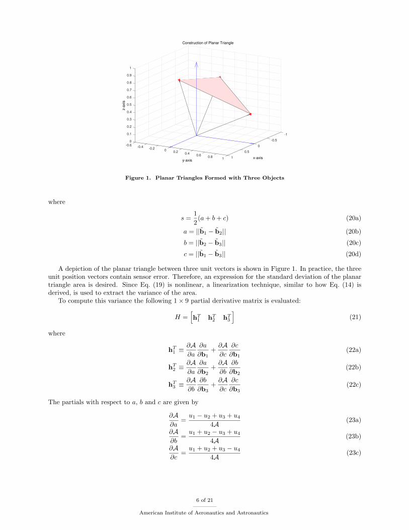
The two properties used by the PTM to identify the objects in the FOV are area and polar moment ofthe planar triangles. The area of the planar triangle can be given by the Heron’s formula.10 Given threeunit vectors pointing toward three space objects, denoted by b1, b2 and b3, the area of a planar triangle isgiven by

A =√s (s− a) (s− b) (s− c) (19)

5 of 21


-1

-0.50

Construction of Planar Triangle

0.1

0.2

-0.6

x-axis

0

0.3

-0.4

0.4

0.5

-0.2

z-a

xis

0.6

0.7

0

y-axis

0.8

0.50.2

0.9

1

0.40.6

0.8 11

Figure 1. Planar Triangles Formed with Three Objects

where

s =1

2(a+ b+ c) (20a)

a = ||b1 − b2|| (20b)

b = ||b2 − b3|| (20c)

c = ||b1 − b3|| (20d)

A depiction of the planar triangle between three unit vectors is shown in Figure 1. In practice, the threeunit position vectors contain sensor error. Therefore, an expression for the standard deviation of the planartriangle area is desired. Since Eq. (19) is nonlinear, a linearization technique, similar to how Eq. (14) isderived, is used to extract the variance of the area.

To compute this variance the following 1× 9 partial derivative matrix is evaluated:

H =[hT1 hT

2 hT3

](21)

where

hT1 ≡

∂A∂a

∂a

∂b1+∂A∂c

∂c

∂b1(22a)

hT2 ≡

∂A∂a

∂a

∂b2+∂A∂b

∂b

∂b2(22b)

hT3 ≡

∂A∂b

∂b

∂b3+∂A∂c

∂c

∂b3(22c)

The partials with respect to a, b and c are given by

∂A∂a

=u1 − u2 + u3 + u4

4A(23a)

∂A∂b

=u1 + u2 − u3 + u4

4A(23b)

∂A∂c

=u1 + u2 + u3 − u4

4A(23c)

6 of 21


where

u1 = (s− a) (s− b) (s− c) (24a)

u2 = s (s− b) (s− c) (24b)

u3 = s (s− a) (s− c) (24c)

u4 = s (s− a) (s− b) (24d)

The partials with respect to b1, b2 and b3 are given by

∂a

∂b1= (b1 − b2)

T/a,

∂a

∂b2= − ∂a

∂b1(25a)

∂b

∂b2= (b2 − b3)

T/b,

∂b

∂b3= − ∂b

∂b2(25b)

∂c

∂b1= (b1 − b3)

T/c,

∂c

∂b3= − ∂c

∂b1(25c)

The variance of the area, denoted by σ2A, is given by

σ2A = H RHT (26)

where

R ≡

R1 03×3 03×3

03×3 R2 03×3

03×3 03×3 R3

(27)

where 03×3 denotes a 3×3 matrix of zeros and R1, R2 and R3 are given by Eq. (18). Note that the matricesH and R are evaluated at the respective true values; however, replacing the true values with the measuredones leads to second-order errors that are negligible. Since the standard deviation, σA, is derived analytically,the bounds over which the true area is likely to exist can be determined precisely to within any prescribedconfidence level, no matter the shape or size of the planar triangle.

The triangular polar moment of inertia is introduced as a supplemental screening property to the planartriangle area. If two planar triangles have the same area, then their polar moments are most likely different.The reverse is also true; if two planar triangles have the same polar moments, then it is likely that their areasare not equal. The polar moment of inertia property helps further differentiate possible triangle combinations.The polar moment of inertia the planar triangle is given by

J = A (a2 + b2 + c2)/36 (28)

As with the area, the variance of the polar moment of inertia can also be derived in closed form. To computethis quantity the following 1× 9 partial derivative matrix is evaluated:

H =[hT1 hT

2 hT3

](29)

where

hT1 ≡

∂J∂a

∂a

∂b1+∂J∂c

∂c

∂b1+∂J∂A

hT1 (30a)

hT2 ≡

∂J∂a

∂a

∂b2+∂J∂b

∂b

∂b2+∂J∂A

hT2 (30b)

hT3 ≡

∂J∂b

∂b

∂b3+∂J∂c

∂c

∂b3+∂J∂A

hT3 (30c)

with

∂J∂a

= A a/18,∂J∂a

= A b/18,∂J∂a

= A c/18 (31a)

∂J∂A

= (a2 + b2 + c2)/36 (31b)

7 of 21


All other quantities in Eq. (30) are given from the area variance calculations. The variance of the polarmoment of inerita, denoted by σ2

J , is given by

σ2J = H R HT (32)

As with the area variance, the true values are replaced with the respective measured polar moment of inertia.

Figure 2. Flattened Spherical Quad-Tree Structure

A. Planar Triangle Catalog

It is necessary to organize the planar triangle catalog in an efficient manner to help reduce search andcreation time. This is especially important because, unlike stars, RSO catalogs are updated frequently(sometimes daily). Therefore, a new planar triangle catalog will need to be created once an RSO catalog ismade available. In order to make the catalog easily accessible, a spherical quad-tree structure is used. Thespherical quad-tree structure is similar to a traditional quad-tree structure except it uses spherical trianglesinstead of square quadrants as the element type. The traditional quad-tree is presented in detail in Ref. 19.A spherical quad-tree structure is a multi-level apportioned spherical triangle that enables objects to beassociated based on their location within that spherical triangle. If the spherical triangle is flattened in 2-Dspace, then it would somewhat resemble the triangular structure shown in Figure 2. The spherical triangleis divided into four labeled elements in each of its three levels. Also, each individual element is assignedthree labeled vertices. During the spherical quad-tree build, each object is assigned to a spherical triangleand the associated elements based on its location in the celestial sphere. The elements and vertices are theparameters used to locate a particular object in the structure. There are four spherical triangles that createa spherical tetrahedron that spans the entire celestial sphere. To further simplify the search, only the objectswithin the specified FOV are considered. Therefore, any object outside this boundary is omitted from thesearch.

During a search it is not immediately known where each object is located since there are a significantnumber of them cataloged. To clarify the search process, an example will be presented. Assume that anyobject in space, denoted as star A in Figure 2, is the only object cataloged, and it is located inside root(top level) − element 1, level 1 − element 7, level 2 − element 11, and level 3 − element 13. Now, supposemeasurements are taken and the measured angle lies within a boundary of the spherical triangle, say thelower right of element 1. Considering more levels, the measured angle is determined to lie within element13. Since star A is contained in element 13, star A is the measured object. If the measured angle lies withina different boundary and other objects are cataloged, then a different object may be identified. Clearly, itis necessary to define multiple levels in order to obtain a sufficient amount of precision when the number of

8 of 21


objects is large. The benefit of the spherical quad-tree structure is that once it is created, an object can beidentified without using any information about the unit position vector of the object.

The spherical quad-tree is an efficient way to store information, but an optimal organization of thecatalog is desired. If the catalog can be organized in such a way that it follows a mathematical equation,then it would be simple to find a particular property in the catalog. For example, if it is determined thatthe planar triangle area is within a certain boundary, then a search of the catalog for that boundary wouldbe required. If the catalog is not organized appropriately, then it would result in a search spanning themajority of the catalog. Since the catalog can be quite extensive, this would lead to a high computationcost. To resolve this issue the k-vector approach20 is used. For object pattern recognition, if the area of eachpair of objects is plotted against its location in the catalog, then a line can be drawn connecting the firstand last pair of objects. The equation of this line can be used in association with the generated k-vector tolocate where in the catalog a particular pair of objects with a given angle is located. This greatly reducesthe computational burden since the object pattern search algorithm requires a search of the pairs of objectsonly within a measurement uncertainty region, not a search of the entire catalog. For the planar triangleapproach a parabolic k-vector is constructed because it is the best relationship between the planar triangleidentifier and the planar triangle area. If a certain planar triangle area is desired, then the k-vector willquickly provide the associated planar triangle identifier.

−4 −3 −2 −1 0 1 2 3 4−4

−3

−2

−1

0

1

2

3

4

First SphericalTriangleFirst Pivot

Triangle

Figure 3. Pivoting within Field of View

B. Planar Triangle Pivot

If several objects are within the FOV, then it is likely that there can be multiple solutions to the search. Toreduce and ultimately eliminate multiple solutions, planar triangle pivoting is leveraged. The method forpivoting planar triangles is similar to the method for pivoting angles using two objects. A planar triangleis made from three objects in the FOV, and its area and polar moment of inertia are calculated. A rangeover which the true area and polar moment of inertia exist are calculated using the standard deviations foreach. Going through the catalog, triangles that have an area and polar moment that fit within the boundscalculated for the triangle in the FOV are sought. Ideally, only one possible solution exists, but this istypically unlikely. When more than one solution exists, a pivot is performed. Another planar triangle ismade from the objects in the FOV such that there are two objects in common with the first triangle, asshown in Figure 3. A list of possible solutions is made, and then the solutions between the first planartriangle and second planar triangle are compared. Any solution in each list that does not have two objects incommon with at least one solution in the other lists is discarded. After the comparison is made, if more thanone solution exists, then another pivot is made. Pivoting continues until either a single solution is found orthe pivoting limit has been met. Pivoting such that only one object is shared between the first and second

9 of 21


planar triangles can be done, but would be less effective. The number of triangles that are likely to shareone object is greater than two, so the solution would require a greater number of pivots.

Also considering false objects and highly cluttered object patterns, the pivoting order would ideally pivotaway from objects that are uncertain. This concept becomes feasible with the addition of the gating methodresults. Careful ordering of the pivoting of the objects in the FOV allows the PTM to strategically pick thenext object to pivot.

IV. Traditional Data Association Methods

Nearest Neighbor (NN) is the simplest data association algorithm, used for single target tracking. Whenmultiple measurements fall within a target’s validation gate, the one that is closest with respect to a pre-defined distance measure is assumed to come from that target. Sometimes called the optimal assignmentapproach, global nearest neighbor (GNN) is the multi-target version of the NN approach. Instead of mini-mizing a single distance, GNN looks to minimize a global distance measure. Two assumptions are made: 1)each measurement can only be associated to one track, and 2) each track can only be associated with onemeasurement. The primary advantage of the GNN algorithm is that its computational cost does not increaserapidly as the number of targets increases. The disadvantage of this algorithm is that track initiation mustbe performed separately. Reference 21 identifies two classes of track initiation techniques: sequential andbatch. The former is preferred for low-clutter environments, while the latter is used for high-clutter envi-ronments. The primary difference between the two is that batch techniques are generally slower and morecomputationally expensive.

The goal of this work is to associate RSOs within a single object field observation. For this reason theNN approach is used as the data association method for gating. This helps to keep away any undesirableobservation that might be made. A simple example of a gating method is that of a house with an auto-matic gate that opens only when the identity of the person at the gate can be verified. However, if theidentity cannot be verified, then the person does not have access. Similarly, validation gates do not let themeasurement be associated with the track if the measurement does not pass the gate provided by the truthand assumed uncertainty. A gate is formed about the predicted measurement, and all observations that fallwithin the gate are considered for the track update. The manner in which the observations are actuallychosen to update the track depends on the data association method in use. Gating methods are useful forreducing complexity and increasing computational efficiency.

A. Elliptical Gates

The Mahalanobis distance is synonymous to the ellipsoidal gate. This is a statistical tool used to measurethe distance between points in multivariate data. Mahalanobis distance measure is also the distance betweena point P and a distribution D. The Mahalanobis distance was originally developed for use with multivariatenormal distributed data. A prediction ellipse is a region for predicting the location of a new observation underthe assumption that the population is bivariate normal. For example, an 80% prediction ellipse indicates aregion that would contain about 80% of the new samples that are drawn from a bivariate normal populationwith mean and covariance matrices that are equal to the sample estimates. The Mahalanobis distance isalso said to be the simple Euclidean distance, which takes into account the covariance of the data. If thecovariance of the data is an identity matrix, then the Mahalanobis distance is equivalent to the Euclideandistance. The Mahalanobis distance measure used in this work is mathematically written as:

dij =√eTijR

−1i eij (33)

where Ri is given by Eq. (18), and the residual eij is given by eij = bj− bi, with bi = Ari, where ri is givenby Eq. (16). Note that dij is computed for all possible (i, j) pairs. The Mahalanobis distance from Eq. (33)represents the general arbitrarily oriented ellipsoid. A ellipsoid with center at v is defined by solutions to xof the equation

(x− v)TZ(x− v) = 1 (34)

where Z is a positive definite matrix. The equation of an ellipse given by Eq. (34) and the Mahalanobisdistance are clearly identical in form, and hence the Mahalanobis distance is often referred to as eitherelliptical gates or ellipsoidal gates.

10 of 21


In the simplest of terms the Mahalanobis distance is a powerful method for measuring how similar someset of conditions are to an ideal set of conditions. This is precisely what is desired by the RSO data associationproblem, because it is desired to see how similar a point in space is to all true points in the catalog. Unlikethe Euclidean distance the Mahalanobis distance takes into account the following facts:

• It accounts for the fact that the variance is different in each direction;

• It accounts for the covariance between variables;

• It reduces to the Euclidean distance for uncorrelated variables and unit variance.

It is desired to determine the probability that the measurement lies inside the following quadratic hyper-surface:

eTijR−1i eij < γ2 (35)

The probability of a correct match is defined by the gate threshold γ. This area is called the validationgate, and the threshold value for γ can be obtained from the inverse χ2 cumulative distribution. The solidellipsoid of values satisfying

(bj − bi)TR−1i (bj − bi) ≤ χ2

n(α)

has probability 1 − α. For example, for three-variable vectors (n = 3), and α = 0.1, then χ2n(α) = 6.2513,

which is what is used in this work.The Mahalanobis distance takes into account factors such as uncertainty and correlations between mea-

surements. Therefore it is an effective tool to solve the RSO data association problem. It will also be shownthat elliptical gates can be used to increase the performance of the PTM. This distance can be combined withalgorithms such as the NN to associate closest neighbors in a multivariate data set. The NN maintains thesingle most likely hypothesis. The fundamental concept of the NN is to associate the most likely assignmentof an measurement to its existing estimate. This association is attained by verifying if the measurement liesin the validation gate and it is the closest measurement to the existing estimate. The NN in the validationgate region is then assigned to the existing estimate, and this is updated.

The NN algorithm can be used with various types of distances (Euclidean, city block, Chebyshev, etc.).The most popular among these is the Mahalanobis distance or the ellipsoidal gate described in this section.The gate can be written in general by

Gr = {z : D(z) ≤ γ} (36)

where D(z) is the distance measure. For the RSO association problem the Mahalanobis distance is usedas the distance measure. Also, z is the estimate, which is determined by propagating the state model ofthe target forward to the observation time. The measurements are associated to the estimates by the NNdetermination through

z∗ = Dargminjij

(z), j = 1, 2, . . . , N (37)

where N is the number of available observations. The subscripts i and j denote eij with corresponding Ri.Application of NN approach for RSO association when a measurement is available involves finding all theneighbors for a given measuremment. This measured value is then associated to the nearest vector in thedata. This simple form of data association will be used for associating a single object to its true object. TheNN approach can be implemented by the following algorithm:

1. Compute the Mahalanobis distance from all possible cataloged estimates to all measurements in theFOV;

2. Accept the closest measurement that passes the gate threshold;

3. Find the match with the lowest Mahalanobis distance for each estimate (ensure only one measurementis associated with each estimate);

4. Update the match as if it were the correct measurement.

11 of 21


V. Simulation Results

To simulate realistic conditions data from the debris field of the 2007 Chinese anti-satellite missile test ofthe Fengyun 1C satellite is used. This Chinese weather satellite was launched into a Sun-synchronous orbitwith a mean altitude of 850 km and an inclination of 98.8 degrees.22 The orbital elements of the 2,000 piecesof debris data for the Fengyun 1C are available on www.celestrak.com. Another set of 2,000 pieces of debrisare also simulated to create a sufficient cluttered environment that stresses the data association algorithms.

The chosen site is the Ground-based Electro-Optical Deep Space Surveillance (GEODSS) instrument,which is located at the White Sands Missile Range in New Mexico. The location of the telescope is 32.82◦

latitude, −106.66◦ longitude and 1.250 (km) altitude. The simulated objects are normally distributed aboutthe specific object in the Fengyun 1C debris field that has the smallest separation angle with respect to thenormal vector of the site at a specific time. This provides a distribution of 2,000 simulated objects in whichthe majority are within the view of the site. In total, there are 4,000 RSOs that are cataloged and roughly2,000 of those are in view of the site.

Simulated objects in ECI coordinates are shown in Figure 4. The ECI initial debris data are thenpropagated to obtain an instance of time in which there is an acceptable amount of debris visible to the site.Then the debris is converted to the ECEF coordinate system. To see RSOs in the FOV, transformationsfrom ECEF to ENU to the INSTR frame are required. The reader is recommended to review Ref. 2 (chapter5), for details of the simulations required to generate the RSO.

-6000

-4000

-2000

6000

0

4000

z-a

xis

(km

) 2000

2000

4000

5000

Initial Debris Positions (ECI)

y-axis (km)

6000

0

x-axis (km)

-2000 0-4000

-6000 -5000-8000

Figure 4. Debris in ECI Coordinate System

A. Planar Triangle Method Algorithm

The PTM code execution can be seen in Ref. 10. However a broad overview of the steps can be given asfollows:

1. Create the spherical quad-tree structure;

2. Catalog planar triangles;

3. Add planar triangle properties;

4. Sort planar triangles;

5. Run the pattern recognition algorithm in a Monte Carlo regime.

The first step in the PTM code execution is to create a multi-level spherical quad-tree structure. Then,based on an RSO’s position data, it is stored within that structure. Once all RSOs have been assigned aposition in the tree structure, the planar triangle properties are computed and associated with that tree

12 of 21


structure location. To increase efficiency further, a binary tree is implemented to sort the planar triangleproperties according to the value of the planar triangle area. The ultimate goal is to provide an efficientstoring mechanism that can be used to quickly associate an RSO based on planar triangle area and polarmoment.

Once the storing mechanism (steps 1-4) has been constructed, it can now be used to compare focal-planeobservations of RSOs from the catalog. Several Monte Carlo runs are executed to test the PTM. At eachiteration, a random telescope boresight is generated, and an associated random INSTR frame is constructed.From this INSTR frame, all RSOs within the FOV are provided as inputs to the pattern recognition algo-rithm. This sequence is repeated many times in order to accumulate a large result set. A representation ofthe pattern recognition algorithm is as follows:

for i = 1 to number of desired iterations do

• Compute random boresight vector;

• Compute random INSTR frame with tz aligned with boresight vector;

• Determine RSOs in FOV;

• Perform ENU to INSTR coordinate system transformation;

• Compute focal-plane observations;

• Add sensor error to focal-plane observations;

• Compute measured RSO position vectors with both measurement and sensor error;

• Compute planar triangle properties;

• Compute area variance;

• Compute polar moment variance;

• Compare computed values with catalog and determine matching RSOs.

The first step in the algorithm is to compute a random boresight vector. This represents a randomtelescope boresight, which is restricted to the physical attributes of the space surveillance telescope. Thetelescope is restricted to an elevation angle of 20 degrees above the horizon and an azimuth angle that spansthe entire plane. Therefore the random boresight vectors are uniformly distributed within these boundaries.The random boresight vector is computed by

θelev =π

9+[π

2− π

9

]rand(1) (38a)

ψaz = 2π rand(1) (38b)

rb =

cos(θelev) cos(ψaz)

cos(θelev) sin(ψaz)

sin(ψaz)

(38c)

In the above equation, θelev and ψaz are the elevation and azimuth angles, respectively. The function rand isuniform random number generator. The random INSTR frame is then constructed with the tz axis alignedwith the current boresight vector.

The INSTR frame is constructed by:

tz = rb (39a)

t′y = tz × r′b (39b)

ty =tz × t′y‖tz × t′y‖

(39c)

tz =ty × tz‖ty × tz‖

(39d)

13 of 21


where r′b is a separate random vector generated from Eq. (38c), and t′y is a temporary y-axis used to generatethe orthogonality condition between tz and ty. The specific orientation of the txy plane is not significantas long as tz is along the boresight vector. The instrument is assumed to have a 6 degree FOV, which isrepresented by a plane at the end point of the random boresight vector. The condition for an object to bewithin the FOV is given by

arccos(rRSO · rb) ≤3π

180(40)

B. Execution of PTM

For the purpose of simulation 1,000 random boresight vectors are generated. The RSOs in the FOV for eachboresight vector are calculated, and when the RSOs in FOV are more than the minimum number desired,the PTM is executed. Two Monte Carlo runs of random attitude tests (RATs) are performed − each MonteCarlo run consists of 1,000 RATs, and this Monte Carlo simulation is done two times for every case ofmeasurement error. An illustration of the random boresight vectors computed with the debris can be seenin Figure 5, which gives a clear understanding of how the boresight vectors are generated, and also helpsto visualize the RSOs that are within the FOV. In Figure 5 the red dots are the debris in space. The bluestraight lines pointing up towards the debris are the boresight vectors of the telescope. The blue lines at thebase of the boresight vectors show the other two axes of each boresight vector. The blue circular head ontop of each boresight vector is the FOV for that particular telescope boresight, and the light pink trianglesare the planar triangles formed between the debris pieces in space. For the purpose of simulations, six casesof measurement error are used listed in Table 1.

Figure 5. Random Attitude Tests with Debris

Table 1. Measurement Errors

Iteration no. 1 2 3 4 5 6

3σ errors (km) 0.06 0.12 0.24 0.3 0.6 0.9

C. Gating-Based Data Association

Gating-based data association involves the association of measurements to known true values or tracks, andthe sorting of results based on the data association method. As mentioned the data association methodfor this simulation is the NN method. In order to evaluate the performance of this algorithm with respectto object association, randomly selected FOVs in the aforementioned object measurement and catalog areselected and used as an input to the gating method. Figure 6 shows the number of debris objects visible to

14 of 21


the ground site for a representative single run. The Mahalanobis distance between each measured observationand all its true positions are found. Then the NN algorithm is used to associate the closest measured valueto the true debris. Another logical check is performed to ensure that only one measurement is associatedwith a single track. If more than one association is made to a true track, then the measurement with thelowest Mahalanobis distance is chosen. At the output of each association, a check is performed to see ifthe associated objects match the true objects. If both the measured and truth are the same, then a correctmatch is counted and the truth counter is incremented, else a bad/fail counter is incremented.

Figure 6. Debris in the FOV

D. Cluttering the FOV to Test Gating and PTM

Since the gating method performs exceptionally well in cases where the FOV is very lightly dense, the systemis strained for cases where the FOV is very dense, or cluttered with debris. A function is used to artificiallyadd pieces of debris in the FOV. To add closely spaced debris the pairwise distance between each piece ofdebris in the FOV is taken. The minimum distance in each case is taken and used as the 3σ (standarddeviation) to generate three pieces of debris around each already existing debris to populate the FOV, asshown in Figure 7. This figure illustrates the cluttering approach used to demonstrate performance of theproposed algorithms. Once the addition of debris is done, the simple elliptical gating approach is used forthe debris matching, and the results are saved accordingly.

VI. Gating-Assisted Planar Triangular Method

This method couples the working of the PTM and the gating method. First, the gating method isexecuted as a precursor to the PTM. Here, the gating method is used to associate the measured data to thetruth data under varying measurement errors. Once gating data associations are completed, the PTM isexecuted using the updated track values determined in the gating process.

The pre-processing of the measurement field with the gating data association helps the PTM to comparedebris pieces that are already associated to the truth. In the case where the gating process incorrectlymatches a measurement to the wrong track, the PTM algorithm has additional criteria in the triangleproperties to screen mismatches. The polar moment of inertia provides additional screening criteria toevaluate observations determined in the gating processing. When considering the flexibility to use thepivoting methods, the PTM acts as a robust additional screening method for gating results.

Additional performance can be realized by providing an intelligent pivoting order based on the outputof the gating results. If there are sufficient gating-associated objects, then the combinations of associatedobjects are determined, and then they are sorted based on triangle area. The sorted results are re-organizedto follow the traditional pivot method where one object of the triangle is shifted from the first to the nextanalysis. This approach allows the PTM to use more information yielded from gating to assist in determiningprecise and robust object association. If more pivots are available, then the objects in the FOV that arenot associated by gating can fill out the remainder of the pivots. Along with the updated object vectors,

15 of 21


-3 -2 -1 0 1 2 3-3

-2

-1

0

1

2

3Field of View

Center of FOV

FOV

True Position

Measured Position

Figure 7. Adding Three Pieces of Debris Around Each Existing Piece to Clutter the Environment

the pre-sorted pivot list is handed over to the traditional PTM algorithm. Once the PTM is executed theresults obtained are saved for each run. Results below show that this method increases the efficiency andeffectiveness of the PTM under highly cluttered and uncertain conditions.

The gating-assisted PTM object association method is summarized as follows:

• Perform gating data association with measured objects in the FOV;

• Update measured tracks with associated vectors based on the output of the gating method;

• Determine triangles and planar triangle area based on the combinations of the observations;

• Sort the area of the triangles in descending order;

• Starting with the largest area, re-sort triangles based on pivoting logic used in the PTM approach;

• Using the pivoting list and updated track vectors, execute the PTM algorithm to determine objectmatches.

Outputting a failed result from the PTM given incorrectly associated objects in the gating pre-processing isalmost as good as a correct output from the PTM. By signifying a failure given incorrect observations, thePTM acts as a screen previously unavailable to the gating method alone. Without the PTM addition, thegating method can supply incorrect matches without any additional checks.

By prioritizing the inputs of the PTM with the results of the gating method, notable improvements tothe stand-alone performance of both algorithms are realized. The synergistic result of joining these twomethods yields improvements than either alone. The PTM benefits from the prioritization of results fromgating because it does not have to pivot through uncertain measurements. The gating method benefits fromthe robustness of the PTM because the PTM can correct and/or reject incorrect associations made fromgating. The gating-assisted PTM is also shown to perform well under highly populated false object cases.

A. Results

The purpose of this work is to show that the accuracy of the PTM can be improved by using elliptical gatesas a screening method to associate the measured observations to the truth. A comprehensive study has alsobeen performed on using just the gating approach for data association. During the study it is found thatthe simple gating approach works well in cases where the FOV is not cluttered with debris and corrupted byuncertainty. The simple gating approach for an uncluttered FOV proves to have a better performance under

16 of 21


varying uncertainty in the debris position, when compared to the PTM. But when left without additionalscreening, the gating method yields more incorrect associations.

Figure 8 shows the accuracy of the gating method compared to the PTM. Note that each run numberrepresents 1,000 Monte Carlo runs. The gating method is very promising in an uncluttered regime, whileboth algorithms tend to be sensitive to measurement uncertainty. The uncluttered condition is useful as abaseline, but to stress the algorithms, the FOV is artificially cluttered with additional debris.

0.06 0.06 0.12 0.12 0.24 0.24 0.3 0.3 0.6 0.6 0.9 0.9

Measurement Error [km]

0

10

20

30

40

50

60

70

80

90

100

Success P

erc

enta

ge

PTM vs Gating Method in Uncluttered FOV

PTMGating

Figure 8. Accuracy of the Gating Method Compared to the PTM in an Uncluttered FOV

Table 2. x-Axis Run Number and Corresponding Measurement Error

Run No. 1, 2 3, 4 5, 6 7, 8 9, 10 11, 12

RSO Meas. 3σ Error (km) 0.06 0.12 0.24 0.3 0.6 0.9

The performance of the object association algorithms decrease when presented with a highly clutteredenvironment. As expected the accuracy of the gating method becomes more sensitive to noise as performancesuffers with the increase in measurement uncertainty. As the measurement uncertainty ellipse and the tightlycluttered measurements start to overlap, the ability of either algorithm to associate the likely object dropssignificantly. The cluttered FOV case is run for both the gating and PTM algorithms, and results arecompared. In Figure 9, the PTM results show significant sensitivity to the highest measurement case. Bothalgorithms take a hit to performance and show increased sensitivity to uncertainty.

To investigate the performance further, Figures 10(a) and 10(b) illustrate the minimum pairwise distancemeasured in each FOV run in the cluttered case where the respective algorithm fails to produce the correctobject association. Clearly, the tightly spaced and cluttered FOV is the leading cause of failure in the twoalgorithms. The separation distance at which both algorithms degrade is well below the average distancemeasured in the FOV.

To improve upon the performance of the gating and PTM, the gating-assisted PTM is evaluated. Asdescribed above in Section VI, the gating-assisted PTM utilizes the gating algorithm as a precursor to thePTM. When this gating method is performed before the PTM, significant robustness to noise and uncertaintyis shown. The results shown in Figure 11 show clear improvement of performance of the new method to thatof the previously existing PTM or gating. It can be seen that the PTM with gates performs better thanthe PTM alone. The PTM with gating pre-processing shows an improvement over gating and PTM alonethat gets better with increasing measurement uncertainty. To show the combined approach is statisticallysignificant a hypothesis test is performed. In this method it is found that the null hypothesis shows themethods are identical in performance at the 99% confidence interval. After performing the hypothesistesting, the null hypothesis was rejected. This confirms the assumption that the application of gating to thePTM helps enhance the overall association performance.

17 of 21


0.06 0.06 0.12 0.12 0.24 0.24 0.3 0.3 0.6 0.6 0.9 0.9


0

10

20

30

40

50

60

70

80

90

100

Success P

erc

enta

ge

Planar Triangle Method vs Gating Method in Highly Cluttered FOV

PTMGating

Figure 9. Comparision of PTM with the Gating Method for Varying Measurement Errors

0 5 10 15

Minimum Distance Between Debris×10

-3

0

50

100

150

200

250

300

350

400

450

500

Occu

rre

nce

of

Fa

ilure

/In

co

rre

ct

ID

Minimum Distance of Failure/Incorrect PTM ID in Highly Cluttered FOV

Average Distance: 0.041276

PTM Incorrect ID

(a) Min Distance of Failed Cases, PTM

0 5 10 15

Minimum Distance Between Debris×10

-3

0

50

100

150

200

250

300

350

Occu

rre

nce

of

Fa

ilure

/In

co

rre

ct

ID

Minimum Distance of Failure/Incorrect Gating ID in Highly Cluttered FOV

Average Distance: 0.041342

Gating Incorrect ID

(b) Min Distance of Failed Cases, Gating

Figure 10. Minimum Distance Analysis for Failures on PTM and Gating Methods in Cluttered Environments

The breakdown of the gating-assisted PTM performance against incorrect associations from the gatingpre-processing shows the power of pivoting and of the pre-sorted pivoting index. The inclusion of the PTMallows for a significant reduction in false associations when compared to the gating-only method. For allcases, the PTM is able to correct the incorrect gating associated measurements at a rate of over 95%. Figures12(a) and 12(b) illustrate the performance of the gating-assisted PTM as well as how the algorithm handlesincorrect associations from gating. The screening capability of the PTM significantly enhances the successrate of the output by utilizing the planar triangle properties as well as pivoting. The extremely small numberof incorrectly associated object combinations outputted from the gating-assisted PTM is notable given theharsh cluttering and uncertainty condition. The ability to screen and remove bad associations is attributedto the PTM as demonstrated in Ref. 10.

To evaluate the performance of the proposed algorithm in yet another challenging environment, theclutter added to the FOV is not cataloged, therefore the clutter acts as false object observations. Thefalse object could be an uncataloged star/object or a sensor malfunction. It is important to note that theapproach in this work uses “static” (spatial) observations (i.e. one snapshot in the FOV), unlike “dynamic”

18 of 21


0.06 0.06 0.12 0.12 0.24 0.24 0.3 0.3 0.6 0.6 0.9 0.9


0

10

20

30

40

50

60

70

80

90

100

Success P

erc

enta

ge

Method Comparison for Highly Cluttered FOVPTM+Gating CorrectPTM CorrectGating Correct

Figure 11. Performance of Gating-Assisted PTM in Highly Cluttered FOV

0.06 0.06 0.12 0.12 0.24 0.24 0.3 0.3 0.6 0.6 0.9 0.9

Measurement Error

0

10

20

30

40

50

60

70

80

90

100

Perc

enta

ge o

f O

ccurr

ence

Gating-Assisted Planar Triangle Method in Highly Cluttered Cataloged FOV

PTM+GatingGating Incorrect

(a) Gating-Assisted PTM and Incorrect GatingID’s

0.06 0.06 0.12 0.12 0.24 0.24 0.3 0.3 0.6 0.6 0.9 0.9

Measurement Error

0

50

100

150

200

250

300

350

Occu

rre

nce

of

Inco

rre

ct

Ga

tin

g R

esp

on

se

PTM Response Given Incorrect Gating Measurement Association

PTM Correct IDPTM Inconclusive IDPTM Incorrect ID

(b) Breakdown of PTM Response to Incorrect Gat-ing ID’s

Figure 12. Gating-Assisted PTM Performance with Incorrect Gating ID’s in Highly Cluttered FOV

(temporal) filtering-based methods. Therefore, actual stars in the FOV can be treated as false objects.Clearly by adding three times the number of false objects than the number of real objects, the simulationcase is extremely challenging. The PTM approach alone would unlikely be able to provide any solutiongiven the low probability of selecting real objects out of the FOV, and without using an extraordinarilyhigh pivot limit. But the gating method will help match measurements to existing objects based on theMahalanobis distance. Results show excellent performance of the gating-assisted PTM. Figures 13(a) and13(b) demonstrate the ability of the gating-assisted PTM to overcome significant numbers of false objectsand measurement uncertainty to provide the correct object association. Compared to the true object case,the false object case shows more dependency on measurement noise, but still remains comparable. Again,Figure 13(b) demonstrates the benefit of the hybrid gating-assisted PTM, where incorrect associations fromgating are corrected a majority of the time via the PTM. The false object case shows more conditions wherethe PTM could not achieve an object association given the incorrect gating association. Although not ideal,the rejection of the gating-associated values is still a significant improvement over the gating method alone.

A paired-sample t-test is conducted to compare the mean accuracy of the PTM versus the PTM with

19 of 21


0.06 0.06 0.12 0.12 0.24 0.24 0.3 0.3 0.6 0.6 0.9 0.9

Measurement Error

0

10

20

30

40

50

60

70

80

90

100

Pe

rce

nta

ge

of

Occu

rre

nce

Gating-Assisted Planar Triangle Method in Highly Cluttered False Star FOV

PTM+GatingGating Incorrect Results

(a) Gating-Assisted PTM and Incorrect GatingID’s with False Stars

0.06 0.06 0.12 0.12 0.24 0.24 0.3 0.3 0.6 0.6 0.9 0.9

Measurement Error

0

50

100

150

200

250

300

350

400

Occu

rre

nce

of

Inco

rre

ct

Ga

tin

g R

esp

on

se

PTM Response Given Incorrect Gating Measurement Association

PTM Correct IDPTM Inconclusive IDPTM Incorrect ID

(b) Breakdown of PTM Response to Incorrect Gat-ing ID’s

Figure 13. Gating-Assisted PTM Performance with Incorrect Gating ID’s in Highly Cluttered False Star FOV

gates using the IBM SPSS 19 Statistical Software. The summarized results in Tables 3 − 4 show a significantdifference between the accuracy of PTM with gates (Mean = 91.32, S.D. = 13.164) and PTM alone (Mean =83.52, S.D. = 13.841) with t = 11.415 at p = 0.01. From these results it is concluded that PTM with gatesis 7.801% (Mean = 7.801,S.D. = 2.899) more accurate than PTM alone with a 99% confidence interval.

Table 3. Paired Samples Statistics

Mean N Std. Deviation Std. Error Mean

PTM Gate 91.32 18 13.164 3.103

PTM 83.52 18 13.841 3.262

N Correlation Sig

PTM Gate & PTM 18 0.978 0.000

Table 4. Paired Samples Test for Difference Between PTM Gate and PTM Only

Paired Differences

99 % Confidence Interval

Std. Std. of the Difference Sig.

Mean Deviation Error Mean Lower Upper t df (2-tailed)

7.801 2.899 0.683 5.820 9.782 11.415 17 0.000

VII. Conclusions

This work extends the concepts of using ellipsoidal validation gates to data association and patternrecognition algorithms such the planar triangle method (PTM). The proposed method of using a ellipsoidalgating as a precursor to the PTM shows improvement in accuracy of objects being correctly associated whencompared to the PTM or gating method alone in a highly challenging field of view. This method is fairlysimple and compact in implementation, but the results show a significant improvement ranging anywherefrom 5% to 20% depending on the measurement errors involved. The greatest improvement in successfulobject association is shown in high measurement uncertainty simulations. Due to the lack of a reliablescreening method, the gating method is most likely not a feasible association algorithm on its own. Asuncertainty rises, the gating method yields significantly more incorrect results while the PTM often yields

20 of 21


inconclusive associations. When the gating method is joined with the PTM, a significant improvement inrobustness and accuracy is realized. The synergistic effect of combining the two methods removes certaindisadvantages of each. The PTM provides additional screening and checking to the gating output data, whilethe gating output data provides a verified starting point for the PTM to begin its search. The addition of asmart pivoting index as an output of the gating method proves to increase reliability of the PTM.

VIII. Future Work

Investigation into an even more intelligent and streamlined interface between gating and PTM algorithmscould provide savings in computation and additional increases in accuracy. Potentially, using the Mahalanobisdistance to dictate the next pivot from an unlikely object to a more likely measurement, could provideadditional benefits. Further exploration into data association for non-Gaussian errors could make a strongercase for implementation as orbit errors are often non-Gaussian. More advanced data association techniquescan be used that do not make an assumption of the form of the uncertainty of the measurement.

References

1NASA, “International Space Station Performs Fourth and Fifth Debris Avoidance Maneuvers of 2014,” Orbital DebrisQuaterly News, Vol. 19, NASA, Jan. 2015, pp. 1–2.

2Silversmith, P. E., Space-Object Identification Using Spatial Pattern Recognition, Master’s thesis, University at Buffalo,State University of New York, 2013.

3Hill, K., Alfriend, K. T., and Sabol, C., “Covariance-based Uncorrelated Track Association,” AIAA/AAS AstrodynamicsSpecialist Conference and Exhibit , Honolulu, HI, 2008, AIAA 2008-7211, doi:10.2514/6.2008-7211.

4Giza, D., Singla, P., Crassidis, J., Linares, R., Cefola, P., and Hill, K., “Entropy-Based Space Object Data AssociationUsing an Adaptive Gaussian Sum Filter,” AIAA/AAS Astrodynamics Specialist Conference, Toronto, ON, Canada, 2010, AIAA2010-7526, doi:10.2514/6.2010-7526.

5DeMars, K. J., Hussein, I. I., Frueh, C., Jah, M. K., and Erwin, R. S., “Multiple-Object Space Surveillance Track-ing Using Finite-Set Statistics,” Journal of Guidance, Control, and Dynamics, Vol. 38, No. 9, March 2015, pp. 1741–1756,doi:10.2514/1.G000987.

6Cheng, Y., DeMars, K., and Fruh, C., “Gaussian Mixture PHD Filter for Space Object Tracking,” AAS/AIAA SpaceFlight Mechanics Meeting, Kauai, HI, 2013, AAS 13-242.

7Jones, B. A. and Vo, B.-N., “A Labeled Multi-Bernoulli Filter for Space Object Tracking,” AAS/AIAA Space FlightMechanics Meeting, Williamsburg, VA, 2014, AAS 15-413.

8Holzinger, M. J., “Using Magnetometers for Space Object Characterization in Space Situational Awareness Applications,”Journal of Guidance, Control, and Dynamics, Vol. 37, No. 5, Sept.-Oct. 2014, pp. 1397–1405, doi:10.2514/1.G000523.

9Spratling, B. B. and Mortari, D., “A Survey on Star Identification Algorithms,” Algorithms, Vol. 2, No. 1, Jan. 2009,pp. 93–107, doi:10.3390/a2010093.

10Cole, C. L. and Crassidis, J. L., “Fast Star-Pattern Recognition Using Planar Triangles,” Journal of Guidance, Control,and Dynamics, Vol. 29, No. 1, Jan.-Feb. 2006, pp. 64–71, doi:10.2514/1.13314.

11Blackman, S. and Popoli, R., Design and Analysis of Modern Tracking Systems, Artech House, Boston, MA, 1999.12Schaub, H. and Junkins, J. L., Analytical Mechnics of Space Systems, American Institute of Aeronautics and Astronautics,

Inc., Reston, Virginia, 2nd ed., 2009.13Light, D. L., “Satellite Photogrammetry,” Manual of Photogrammetry, edited by C. C. Slama, chap. 17, American Society

of Photogrammetry, Falls Church, VA, 4th ed., 1980.14Vallado, D. A., Fundamentals of Astrodynamics and Applications, Microcosm Press, Torrance, CA, 4th ed., 2013.15Shuster, M. D., “Kalman Filtering of Spacecraft Attitude and the QUEST Model,” Journal of the Astronautical Sciences,

Vol. 38, No. 3, July-Sept. 1990, pp. 377–393.16Shuster, M. D. and Oh, S. D., “Three-Axis Attitude Determination from Vector Observations,” Journal of Guidance and

Control , Vol. 4, No. 1, Jan.-Feb. 1981, pp. 70–77, doi:10.2514/3.19717.17Cheng, Y., Crassidis, J. L., and Markley, F. L., “Attitude Estimation for Large Field-of-View Sensors,” Journal of the

Astronautical Sciences, Vol. 54, No. 3&4, July-Dec. 2006, pp. 433–448.18Hinks, J. C. and Crassidis, J. L., “Covariance Analysis of Maximum Likelihood Attitude Estimation,” The Journal of

the Astronautical Sciences, Vol. 60, No. 2, 2013, pp. 186–210, doi:10.1007/s40295-014-0028-7.19Cole, C. L., Fast Star Pattern Recognition Using Spherical Triangles, Master’s thesis, University at Buffalo, State

University of New York, 2004.20Mortari, D., “A Fast On-Board Autonomous Attitude Determination System Based on a new Star-ID Technique for a

Wide FOV Star Tracker,” AAS/AIAA Space Flight Mechanics Meeting, Austin, TX, 1996, AAS 96-158.21Leung, H., Hu, Z., and Blanchette, M., “Evaluation of multiple target track initiation techniques in real radar tracking

environments,” IEE Proceedings - Radar, Sonar and Navigation, Vol. 143, No. 4, Aug. 1996, pp. 246–254, doi:10.1049/ip-rsn:19960404.

22Johnson, N. L., Stansbery, E., Liou, J.-C., Horstman, M., Stokely, C., and Whitlock, D., “The Characteristics andConsequences of the Break-Up of the Fengyun-1C Spacecraft,” Acta Astronautica, Vol. 63, No. 1, July-Aug. 2008, pp. 128–135,doi:10.1016/j.actaastro.2007.12.044.

21 of 21


Space Object Data Association Using Spatial Pattern Recognition...

Documents

Transcript of Space Object Data Association Using Spatial Pattern Recognition...