arX

iv:0

806.

4627

v2 [

cs.D

B]

21 O

ct 2

008

SP2Bench: A SPARQL Performance BenchmarkMichael Schmidt∗ ♯, Thomas Hornung♯, Georg Lausen♯, Christoph Pinkel♮

♯Freiburg UniversityGeorges-Koehler-Allee 51, 79110 Freiburg, Germany

{mschmidt|hornungt|lausen }@informatik.uni-freiburg.de

♮MTC Infomedia OHGKaiserstrasse 26, 66121 Saarbrucken, Germany

c.pinkel@mtc-infomedia.de

Abstract— Recently, the SPARQL query language for RDFhas reached the W3C recommendation status. In response tothis emerging standard, the database community is currentlyexploring efficient storage techniques for RDF data and evalua-tion strategies for SPARQL queries. A meaningful analysis andcomparison of these approaches necessitates a comprehensive anduniversal benchmark platform. To this end, we have developedSP2Bench, a publicly available, language-specific SPARQL per-formance benchmark. SP2Bench is settled in the DBLP scenarioand comprises both a data generator for creating arbitrarily largeDBLP-like documents and a set of carefully designed benchmarkqueries. The generated documents mirror key characteristics andsocial-world distributions encountered in the original DBLP dataset, while the queries implement meaningful requests on topofthis data, covering a variety of SPARQL operator constellationsand RDF access patterns. As a proof of concept, we applySP2Bench to existing engines and discuss their strengths andweaknesses that follow immediately from the benchmark results.

I. I NTRODUCTION

The Resource Description Framework [1] (RDF) has be-come the standard format for encoding machine-readableinformation in the Semantic Web [2]. RDF databases canbe represented by labeled directed graphs, where each edgeconnects a so-calledsubjectnode to anobjectnode under labelpredicate. The intended semantics is that theobject denotesthe value of thesubject’s propertypredicate. Supplementary toRDF, the W3C has recommended the declarative SPARQL [3]query language, which can be used to extract informationfrom RDF graphs. SPARQL bases upon a powerful graphmatching facility, allowing to bind variables to components inthe input RDF graph. In addition, operators akin to relationaljoins, unions, left outer joins, selections, and projections canbe combined to build more expressive queries.

By now, several proposals for the efficient evaluation ofSPARQL have been made. These approaches comprise a widerange of optimization techniques, including normal forms [4],graph pattern reordering based on selectivity estimations[5](similar to relational join reordering), syntactic rewriting [6],specialized indices [7], [8] and storage schemes [9], [10],[11],[12], [13] for RDF, and Semantic Query Optimization [14].Another viable option is the translation of SPARQL intoSQL [15], [16] or Datalog [17], which facilitates the evaluation

∗The work of this author was funded by DFG grant GRK 806/2

with traditional engines, thus falling back on establishedoptimization techniques implemented in conventional engines.

As a proof of concept, most of these approaches havebeen evaluated experimentally either in user-defined scenarios,on top of the LUBM benchmark [18], or using the BartonLibrary benchmark [19]. We claim that none of these sce-narios is adequate for testing SPARQL implementations in ageneral and comprehensive way: On the one hand, user-definedscenarios are typically designed to demonstrate very specificproperties and, for this reason, lack generality. On the otherhand, the Barton Library Benchmark is application-oriented,while LUBM was primarily designed to test the reasoningand inference mechanisms of Knowledge Base Systems. As atrade-off, in both benchmarks central SPARQL operators likeOPTIONAL and UNION, or solution modifiers are not covered.

With the SPARQL PerformanceBenchmark (SP2Bench)we propose a language-specific benchmark framework specif-ically designed to test the most common SPARQL constructs,operator constellations, and a broad range of RDF data accesspatterns. The SP2Bench data generator and benchmark queriesare available for download in a ready-to-use format.1

In contrast to application-specific benchmarks, SP2Benchaims at a comprehensive performance evaluation, rather thanassessing the behavior of engines in an application-drivenscenario. Consequently, it is not motivated by a single use case,but instead covers a broad range of challenges that SPARQLengines might face in different contexts. In this line, it allowsto assess the generality of optimization approaches and tocompare them in a universal, application-independent setting.We argue that, for these reasons, our benchmark providesexcellent support for testing the performance of engines ina comprising way, which might help to improve the quality offuture research in this area. We emphasize that such language-specific benchmarks (e.g., XMark [20]) have found broadacceptance, in particular in the research community.

It is quite evident that the domain of a language-specificbenchmark should not only constitute a representative scenariothat captures the philosophy behind the data format, but alsoleave room for challenging queries. With the choice of theDBLP [21] library we satisfy both desiderata. First, RDF hasbeen particularly designed to encode metadata, which makes

1http://dbis.informatik.uni-freiburg.de/index.php?project=SP2B

DBLP an excellent candidate. Furthermore, DBLP reflectsinteresting social-world distributions (cf. [22]), and hencecaptures the social network character of the Semantic Web,whose idea is to integrate a great many of small databasesinto a global semantic network. In this line, it facilitatesthedesign of interesting queries on top of these distributions.

Our data generator supports the creation of arbitrarily largeDBLP-like models in RDF format, which mirror vital keycharacteristics and distributions of DBLP. Consequently,ourframework combines the benefits of a data generator forcreating arbitrarily large documents with interesting data thatcontains many real-world characteristics, i.e. mimics naturalcorrelations between entities, such as power law distributions(found in the citation system or the distribution of papersamong authors) and limited growth curves (e.g., the increasingnumber of venues and publications over time). For this reasonour generator relies on an in-depth study of DBLP, whichcomprises the analysis of entities (e.g. articles and authors),their properties, frequency, and also their interaction.

Complementary to the data generator, we have de-signed 17 meaningful queries that operate on top of thegenerated documents. They cover not only the most importantSPARQL constructs and operator constellations, but also varyin their characteristics, such as complexity and result size. Thedetailed knowledge of data characteristics plays a crucialrolein query design and makes it possible to predict the challengesthat the queries impose on SPARQL engines. This, in turn,facilitates the interpretation of benchmark results.

The key contributions of this paper are the following.• We present SP2Bench, a comprehensive benchmark for

the SPARQL query language, comprising a data generatorand a collection of 17 benchmark queries.

• Our generator supports the creation of arbitrarily largeDBLP documents in RDF format, reflecting key charac-teristics and social-world relations found in the originalDBLP database. The generated documents cover variousRDF constructs, such as blank nodes and containers.

• The benchmark queries have been carefully designedto test a variety of operator constellations, data accesspatterns, and optimization strategies. In the exhaustivediscussion of these queries we also highlight the specificchallenges they impose on SPARQL engines.

• As a proof of concept, we apply SP2Bench to selectedSPARQL engines and discuss their strengths and weak-nesses that follow from the benchmark results. Thisanalysis confirms that our benchmark is well-suited toidentify deficiencies in SPARQL implementations.

• We finally propose performance metrics that capturedifferent aspects of the evaluation process.

Outline. We next discuss related work and design decisionsin Section II. The analysis of DBLP in Section III forms thebasis for our data generator in Section IV. Section V gives anintroduction to SPARQL and describes the benchmark queries.The experiments in Section VI comprise a short evaluationof our generator and benchmark results for existing SPARQLengines. We conclude with some final remarks in Section VII.

II. B ENCHMARK DESIGN DECISIONS

Benchmarking. The Benchmark Handbook [23] providesa summary of important database benchmarks. Probably themost “complete” benchmark suite for relational systems isTPC2, which defines performance and correctness benchmarksfor a large variety of scenarios. There also exists a broad rangeof benchmarks for other data models, such as object-orienteddatabases (e.g., OO7 [24]) and XML (e.g., XMark [20]).

Coming along with its growing importance, different bench-marks for RDF have been developed. The Lehigh UniversityBenchmark [18] (LUBM) was designed with focus on infer-ence and reasoning capabilities of RDF engines. However, theSPARQL specification [3] disregards the semantics of RDFand RDFS [25], [26], i.e. does not involve automated reasoningon top of RDFS constructs such as subclass and subpropertyrelations. With this regard, LUBM does not constitute anadequate scenario for SPARQL performance evaluation. Thisis underlined by the fact that central SPARQL operators, suchas UNION and OPTIONAL, are not addressed in LUBM.

The Barton Library benchmark [19] queries implement auser browsing session through the RDF Barton online catalog.By design, the benchmark is application-oriented. All queriesare encoded in SQL, assuming that the RDF data is stored ina relational DB. Due to missing language support for aggrega-tion, most queries cannot be translated into SPARQL. On theother hand, central SPARQL features like left outer joins (therelational equivalent of SPARQL operator OPTIONAL) andsolution modifiers are missing. In summary, the benchmarkoffers only limited support for testing native SPARQL engines.

The application-oriented Berlin SPARQL Benchmark [27](BSBM) tests the performance of SPARQL engines in a pro-totypical e-commerce scenario. BSBM is use-case driven anddoes not particularly address language-specific issues. With itsfocus, it is supplementary to the SP2Bench framework.

The RDF(S) data model benchmark in [28] focuses onstructural properties of RDF Schemas. In [29] graph featuresof RDF Schemas are studied, showing that they typicallyexhibit power law distributions which constitute a valuablebasis for synthetic schema generation. With their focus onschemas, both [28] and [29] are complementary to our work.

A synthetic data generation approach for OWL based ontest data is described in [30]. There, the focus is on rapidlygenerating large data sets from representative data of a fixeddomain. Our data generation approach is more fine-grained, aswe analyze the development of entities (e.g. articles) overtimeand reflect many characteristics found in social communities.

Design Principles.In the Benchmark Handbook [23], fourkey requirements for domain specific benchmarks are pos-tulated, i.e. it should be (1)relevant, thus testing typicaloperations within the specific domain, (2)portable, i.e. shouldbe executable on different platforms, (3)scalable, e.g. it shouldbe possible to run the benchmark on both small and very largedata sets, and last but not least (4) it must beunderstandable.

2See http://www.tpc.org.

For a language-specific benchmark, the relevance require-ment (1) suggests that queries implement realistic requestson top of the data. Thereby, the benchmark should notfocus on correctness verification, but on common operatorconstellations that impose particular challenges. For instance,two SP2Bench queries test negation, which (under closed-world assumption) can be expressed in SPARQL through acombination of operators OPTIONAL, FILTER, andBOUND.

Requirements (2) portability and (3) scalability bring alongtechnical challenges concerning the implementation of thedatagenerator. In response, our data generator is deterministic,platform independent, and accurate w.r.t. the desired sizeofgenerated documents. Moreover, it is very efficient and getsbywith a constant amount of main memory, and hence supportsthe generation of arbitrarily large RDF documents.

From the viewpoint of engine developers, a benchmarkshould give hints on deficiencies in design and implementa-tion. This is where (4) understandability comes into play, i.e. itis important to keep queries simple and understandable. At thesame time, they should leave room for diverse optimizations.In this regard, the queries are designed in such a way that theyare amenable to a wide range of optimization strategies.

DBLP. We settled SP2Bench in the DBLP [21] scenario.The DBLP database contains bibliographic information aboutthe field of Computer Science and, particularly, databases.

In the context of semi-structured data one often dis-tinguishes between data- and document-centric scenarios.Document-centric design typically involves large amountsoffree-form text, while data-centric documents are more struc-tured and usually processed by machines rather than humans.RDF has been specifically designed for encoding informationin a machine-readable way, so it basically follows the data-centric approach. DBLP, which contains structured data andlittle free text, constitutes such a data-centric scenario.

As discussed in the Introduction, our generator mirrors vitalreal-world distributions found in the original DBLP data. Thisconstitutes an improvement over existing generators that createpurely synthetic data, in particular in the context of a language-specific benchmark. Ultimately, our generator might also beuseful in other contexts, whenever large RDF test data isrequired. We point out that the DBLP-to-RDF translation ofthe original DBLP data in [31] provides only a fixed amountof data and, for this reason, is not sufficient for our purpose.

We finally mention that sampling down large, existing datasets such as U.S. Census3 (about 1 billion triples) mightbe another reasonable option to obtain data with real-worldcharacteristics. The disadvantage, however, is that samplingmight destroy more complex distributions in the data, thusleading to unnatural and “corrupted” RDF graphs. In contrast,our decision to build a data generator from scratch allows ustocustomize the structure of the RDF data, which is in line withthe idea of a comprehensive, language-specific benchmark.This way, we easily obtain documents that contain a rich setof RDF constructs, such as blank nodes or containers.

3http://www.rdfabout.com/demo/census/

<!ELEMENT dblp(article|inproceedings|proceedings|book|

incollection|phdthesis|mastersthesis|www) * ><!ENTITY % field

"author|editor|title|booktitle|pages|year|address|journal|volume|number|month|url|ee|cdrom|cite|publisher|note|crossref|isbn|series|school|chapter" >

<!ELEMENT article (%field;) * >...<!ELEMENT www (%field;) * >

Fig. 1. Extract of the DBLP DTD

III. T HE DBLP DATA SET

The study of the DBLP data set in this section lays thefoundations for our data generator. The analysis of frequencydistributions in scientific production has first been discussedin [32], and characteristics of DBLP have been investigatedin [22]. The latter work studies a subset of DBLP, restrictingDBLP to publications in database venues. It is shown that(this subset of) DBLP reflects vital social relations, forminga “small world” on its own. Although this analysis formsvaluable groundwork, our approach is of more pragmaticnature, as we approximate distributions by concrete functions.

We use function families that naturally reflect the scenarios,e.g. logistics curves for modeling limited growth or powerequations for power law distributions. All approximationshavebeen done with theZunZun4 data modeling tool and thegnuplot5 curve fitting module. Data extraction from the DBLPXML data was realized with the MonetDB/XQuery6 processor.

An important objective of this section is also to provideinsights into key characteristics of DBLP data. Although itisimpossible to mirror all relations found in the original data,we work out a variety of interesting relationships, consideringentities, their structure, or the citation system. The insightsthat we gain establish a deep understanding of the benchmarkqueries and their specific challenges. As an example,Q3a,Q3b, andQ3c (see Appendix) look similar, but pose differentchallenges based on the probability distribution of articleproperties discussed within this section;Q7, on the other hand,heavily depends on the DBLP citation system.

Although the generated data is very similar to the originalDBLP data for years up to the present, we can give noguarantees that our generated data goes hand in hand with theoriginal DBLP data for future years. However, and this is muchmore important, even in the future the generated data willfollow reasonable (and well-known) social-world distributions.We emphasize that the benchmark queries are designed toprimarily operate on top of these relations and distributions,which makes them realistic, predictable and understandable.For instance, some queries operate on top of the citationsystem, which is mirrored by our generator. In contrast, thedistribution of article release months is ignored, hence noquery relies on this property.

A. Structure of Document Classes

Our starting point for the discussion is the DBLP DTDand the February 25, 2008 version of DBLP. An extract of

4http://www.zunzun.com5http://www.gnuplot.info6http://monetdb.cwi.nl/XQuery/

the DTD is provided in Figure 1. Thedblp element defineseight child entities, namely ARTICLE, INPROCEEDINGS, . . .,and WWW resources. We call these entitiesdocument classes,and instances thereofdocuments. Furthermore, we distinguishbetween PROCEEDINGS documents, calledconferences, andinstances of the remaining classes, calledpublications.

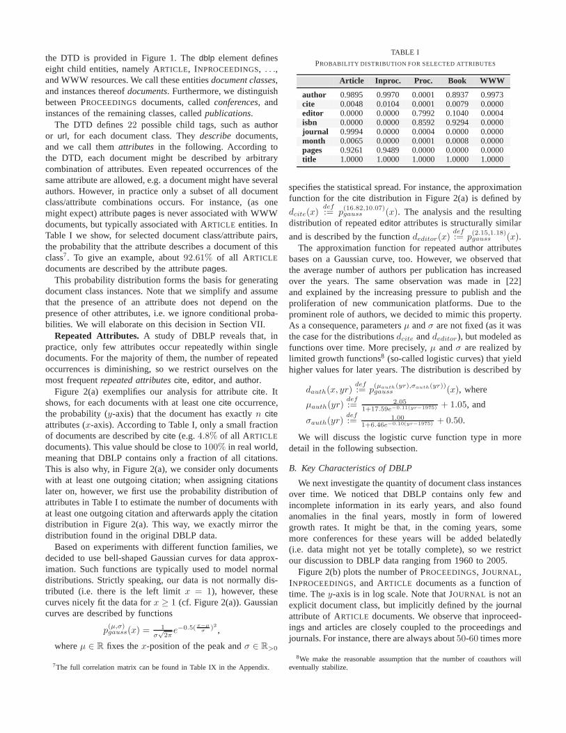
The DTD defines22 possible child tags, such asauthoror url, for each document class. Theydescribedocuments,and we call themattributes in the following. According tothe DTD, each document might be described by arbitrarycombination of attributes. Even repeated occurrences of thesame attribute are allowed, e.g. a document might have severalauthors. However, in practice only a subset of all documentclass/attribute combinations occurs. For instance, (as onemight expect) attributepages is never associated with WWWdocuments, but typically associated with ARTICLE entities. InTable I we show, for selected document class/attribute pairs,the probability that the attribute describes a document of thisclass7. To give an example, about92.61% of all ARTICLE

documents are described by the attributepages.This probability distribution forms the basis for generating

document class instances. Note that we simplify and assumethat the presence of an attribute does not depend on thepresence of other attributes, i.e. we ignore conditional proba-bilities. We will elaborate on this decision in Section VII.

Repeated Attributes. A study of DBLP reveals that, inpractice, only few attributes occur repeatedly within singledocuments. For the majority of them, the number of repeatedoccurrences is diminishing, so we restrict ourselves on themost frequentrepeated attributescite, editor, andauthor.

Figure 2(a) exemplifies our analysis for attributecite. Itshows, for each documents with at least onecite occurrence,the probability (y-axis) that the document has exactlyn citeattributes (x-axis). According to Table I, only a small fractionof documents are described bycite (e.g.4.8% of all ARTICLE

documents). This value should be close to100% in real world,meaning that DBLP contains only a fraction of all citations.This is also why, in Figure 2(a), we consider only documentswith at least one outgoing citation; when assigning citationslater on, however, we first use the probability distributionofattributes in Table I to estimate the number of documents withat least one outgoing citation and afterwards apply the citationdistribution in Figure 2(a). This way, we exactly mirror thedistribution found in the original DBLP data.

Based on experiments with different function families, wedecided to use bell-shaped Gaussian curves for data approx-imation. Such functions are typically used to model normaldistributions. Strictly speaking, our data is not normallydis-tributed (i.e. there is the left limitx = 1), however, thesecurves nicely fit the data forx ≥ 1 (cf. Figure 2(a)). Gaussiancurves are described by functions

p(µ,σ)gauss(x) = 1

σ√

2πe−0.5( x−µ

σ)2 ,

whereµ ∈ R fixes thex-position of the peak andσ ∈ R>0

7The full correlation matrix can be found in Table IX in the Appendix.

TABLE I

PROBABILITY DISTRIBUTION FOR SELECTED ATTRIBUTES

Article Inproc. Proc. Book WWW

author 0.9895 0.9970 0.0001 0.8937 0.9973cite 0.0048 0.0104 0.0001 0.0079 0.0000editor 0.0000 0.0000 0.7992 0.1040 0.0004isbn 0.0000 0.0000 0.8592 0.9294 0.0000journal 0.9994 0.0000 0.0004 0.0000 0.0000month 0.0065 0.0000 0.0001 0.0008 0.0000pages 0.9261 0.9489 0.0000 0.0000 0.0000title 1.0000 1.0000 1.0000 1.0000 1.0000

specifies the statistical spread. For instance, the approximationfunction for thecite distribution in Figure 2(a) is defined by

dcite(x)def:= p

(16.82,10.07)gauss (x). The analysis and the resulting

distribution of repeatededitor attributes is structurally similar

and is described by the functiondeditor(x)def:= p

(2.15,1.18)gauss (x).

The approximation function for repeatedauthor attributesbases on a Gaussian curve, too. However, we observed thatthe average number of authors per publication has increasedover the years. The same observation was made in [22]and explained by the increasing pressure to publish and theproliferation of new communication platforms. Due to theprominent role of authors, we decided to mimic this property.As a consequence, parametersµ andσ are not fixed (as it wasthe case for the distributionsdcite anddeditor), but modeled asfunctions over time. More precisely,µ andσ are realized bylimited growth functions8 (so-called logistic curves) that yieldhigher values for later years. The distribution is described by

dauth(x, yr)def:= p

(µauth(yr),σauth(yr))gauss (x), where

µauth(yr)def:= 2.05

1+17.59e−0.11(yr−1975) + 1.05, and

σauth(yr)def:= 1.00

1+6.46e−0.10(yr−1975) + 0.50.

We will discuss the logistic curve function type in moredetail in the following subsection.

B. Key Characteristics of DBLP

We next investigate the quantity of document class instancesover time. We noticed that DBLP contains only few andincomplete information in its early years, and also foundanomalies in the final years, mostly in form of loweredgrowth rates. It might be that, in the coming years, somemore conferences for these years will be added belatedly(i.e. data might not yet be totally complete), so we restrictour discussion to DBLP data ranging from 1960 to 2005.

Figure 2(b) plots the number of PROCEEDINGS, JOURNAL,INPROCEEDINGS, and ARTICLE documents as a function oftime. They-axis is in log scale. Note that JOURNAL is not anexplicit document class, but implicitly defined by thejournalattribute of ARTICLE documents. We observe that inproceed-ings and articles are closely coupled to the proceedings andjournals. For instance, there are always about50-60 times more

8We make the reasonable assumption that the number of coauthors willeventually stabilize.

0.04

0.03

0.02

0.01

60 50 40 30 20 10 1

prob

abili

ty fo

r x

cita

tions

number of citations = x

probability for number of citationsapprox. probability for number of citations

100k

10k

1k

100

10

2005 2000 1990 1980 1970 1960

num

ber

of d

ocum

ents

in y

ear

x

year = x

proceedingsjournals

inproceedingsarticles

approx. proceedingsapprox. journals

approx. inproceedingsapprox. articles

100000

10000

1000

100

10

80 50 10 5 1

num

ber

of a

utho

rs w

ith p

ublic

atio

n co

unt x

publication count = x

in 1975in 1985in 1995in 2005

approx. for 1975approx. for 1985approx. for 1995approx. for 2005

Fig. 2. (a) Distribution of citations, (b) Document class instances, and (c) Publication counts

inproceedings than proceedings, which indicates the averagenumber of inproceedings per proceeding.

Figure 2(b) shows exponential growth for all documentclasses, where the growth rate of JOURNAL and ARTICLE

documents decreases in the final years. This suggests a limitedgrowth scenario. Limited growth is typically modeled bylogistic curves, which describe functions with a lower and anupper asymptote that either continuously increase or decreasefor increasingx. We use curves of the form

flogistic(x) = a1+be−cx ,

wherea, b, c ∈ R>0. For this parameter setting,a constitutesthe upper asymptote and thex-axis forms the lower asymptote.The curve is “caught” in-between its asymptotes and increasescontinuously, i.e. it isS-shaped. The approximation functionfor the number of JOURNAL documents, which is also plottedin Figure 2(b), is defined by the formula

fjournal(yr)def:= 740.43

1+426.28e−0.12(yr−1950) .

Approximation functions for ARTICLE, PROCEEDINGS, IN-PROCEEDINGS, BOOK, and INCOLLECTION documents differonly in the parameters. PHD THESES, MASTERS THESES,and WWW documents were distributed unsteadily, so wemodeled them by random functions. It is worth mentioningthat the number of articles and inproceedings per year clearlydominates the number of instances of the remaining classes.The concrete formulas look as follows.

farticle(yr)def:= 58519.12

1+876.80e−0.12(yr−1950)

fproc(yr)def:= 5502.31

1+1250.26e−0.14(yr−1965)

finproc(yr)def:= 337132.34

1+1901.05e−0.15(yr−1965)

fincoll(yr)def:= 3577.31

196.49e−0.09(yr−1980)

fbook(yr)def:= 52.97

40739.38e−0.32(yr−1950)

fphd(yr)def:= random[0..20]

fmasters(yr)def:= random[0..10]

fwww(yr)def:= random[0..10]

C. Authors and Editors

Based on the previous analysis, we can estimate the numberof documentsfdocs in yr by summing up the individual counts:

fdocs(yr)def:= fjournal(yr) + farticle(yr) + fproc(yr)+

finproc(yr) + fincoll + fbook(yr)+fphd(yr) + fmasters(yr) + fwww(yr),

Thetotal number of authors, which we define as the numberof author attributes in the data set, is computed as follows.First, we estimate the number of documents described byattributeauthor for each document class individually (using thedistribution in Table I). All these counts are summed up, whichgives an estimation for the total number of documents withone or moreauthor attributes. Finally, this value is multipliedwith the expected average number of authors per paper in therespective year (implicitly given bydauth in Section III-A).

To be close to reality, we also consider the number ofdistinct persons that appear as authors (per year), calleddistinct authors, and the number ofnew authorsin a givenyear, i.e. those persons that publish for the first time.

We found that the number of distinct authorsfdauth peryear can be expressed in dependence offauth as follows.

fdauth(yr)def:= ( −0.67

1+169.41e−0.07(yr−1936) + 0.84) ∗ fauth(yr)

The equation above indicates that the number of distinctauthors relative to the total authors decreases steadily, from0.84% to 0.84%−0.67% = 0.17%. Among others, this reflectsthe increasing productivity of authors over time.

The formula for the numberfnew of new authors builds onthe previous one and also builds upon a logistic curve:

fnew(yr)def:= ( −0.29

1749.00e−0.14(yr−1937) + 0.628) ∗ fdauth(yr)

Publications. In Figure 2(c) we plot, for selected year andpublication countx, the number of authors with exactlyxpublications in this year. The graph is in log-log scale. Weobserve a typical power law distribution, i.e. there are only acouple of authors having a large number of publications, whilelots of authors have only few publications.

Power law distributions are modeled by functions of theform fpowerlaw(x) = axk + b, with constantsa ∈ R>0,exponentk ∈ R<0, andb ∈ R. Parametera affects thex-axisintercept, exponentk defines the gradient, andb constitutesa shift in y-direction. For the given parameter restriction, thefunctions decrease steadily for increasingx ≥ 0.

Figure 2(c) shows that, throughout the years, the curvesmove upwards. This means that the publication count of the

leading author(s) has steadily increased over the last30 years,and also reflects an increasing number of authors. We estimatethe number of authors withx publications in yearyr as

fawp(x, yr)def:= 1.50fpubl(yr)x−f ′

awp(yr) − 5, where

f ′awp(yr)

def:= −0.60

1+216223e−0.20(yr−1936) + 3.08, and

fpubl(yr) returns the total number of publications inyr.Coauthors. In analyzing coauthor characteristics, we inves-

tigated relations between the publication count of authorsandthe number of its total and distinct coauthors. Given a numberx of publications, we (roughly) estimate the average numberof total coauthors byµcoauth := 2.12∗x and the number of itsdistinct coauthors byµdcoauth := x0.81. We take these valuesinto consideration when assigning coauthors.

Editors. The analysis of authors is complemented by astudy of their relations to editors. We associate editors withauthors by investigating the editors’ number of publicationsin (earlier) venues. As one might expect, editors often havepublished before, i.e. are persons that are known in the com-munity. The concrete formula is rather technical and omitted.

D. Citations

In Section III-A we have studied repeated occurrences ofattributecite, i.e. outgoing citations. Concerning theincomingcitations (i.e. the count of incoming references for papers), weobserved a characteristic power law distribution: Most papershave few incoming citations, while only few are cited often.We omit the concrete power law approximation function.

We also observed that the number of incoming citationsis smaller than the number of outgoing citations. This isbecause DBLP contains many untargeted citations (i.e. emptycite tags). Recalling that only a fraction of all papers haveoutgoing citations (cf. Section III-A), we conclude that theDBLP citation system is very incomplete.

IV. DATA GENERATION

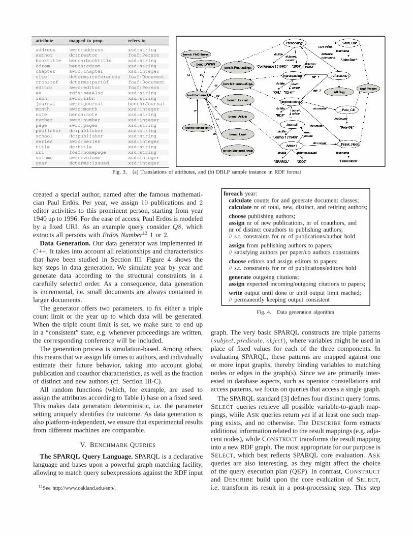
The RDF Data Model. From a logical point of view, RDFdata bases are collections of so-called triples of knowledge.A triple (subject,predicate,object) models the binary relationpredicatebetweensubjectandobjectand can be visualized ina directed graph by an edge from thesubjectnode to anobjectnode under labelpredicate. Figure 3(b) shows a sample RDFgraph, where dashed lines represent edges that are labeled withrdf:type, and sc is an abbreviation forrdfs:subClassOf. Forinstance, the arc from nodeProceeding1to node :John Duerepresents the triple (Proceeding1,swrc:editor, :John Due).

RDF graphs may contain three types of nodes. First,URIs(Uniform Resource Identifiers) are strings that uniquely iden-tify abstract or physical resources, such as conferences orjournals. Blank nodeshave an existential character, i.e. aretypically used to denote resources that exist, but are notassigned a fixed URI. We represent URIs and blank nodes byellipses, identifying blank nodes by the prefix “:”. Literalsrepresent (possibly typed) values and usually describe URIsor blank nodes. Literals are represented by quoted strings.

The RDF standard [1] introduces a base vocabulary withfixed semantics, e.g. defines URIrdf:type for type specifica-tions. This vocabulary also includes containers, such as bagsor sequences. RDFS [25] extends the RDF vocabulary and,among others, provides URIs for subclass (rdfs:subClassOf)and subproperty (rdf:subPropertyOf) specifications. On top ofRDF and RDFS, one can easily create user-defined, domain-specific vocabularies. Our data generator makes heavy use ofsuch predefined vocabulary collections.

The DBLP RDF Scheme. Our RDF scheme basicallyfollows the approach in [31], which presents an XML-to-RDFmapping of the original DBLP data. However, we want togenerate arbitrarily-sized documents and provide lists offirstand last names, publishers, and random words to our datagenerator. Conference and journal names are always of theform “Conference$i ($year)” and “Journal$i ($year)”, where$i is a unique conference (resp. journal) number in year$year.

Similar to [31], we use existing RDF vocabularies to de-scribe resources in a uniform way. We borrow vocabulary fromFOAF9 for describing persons, and from SWRC10 and DC11

for describing scientific resources. Additionally, we introducea namespacebench, which defines DBLP-specific documentclasses, such asbench:Book and bench:Article . Fig-ure 3(a) shows the translation of attributes to RDF properties.For each attribute, we also list its range restriction, i.e.the typeof elements it refers to. For instance, attributeauthor is mappedto dc:creator, and references objects of typefoaf:Person .

The original DBLP RDF scheme neither contains blanknodes nor RDF containers. As we want to test our queries ontop of such RDF-specific constructs, we use (unique) blanknodes “:givennamelastname” for persons (instead of URIs)and model outgoing citations of documents using standardrdf:Bag containers. We also enriched a small fraction ofARTICLE and INPROCEEDINGSdocuments with the new prop-erty bench:abstract (about1%, keeping the modification low),which constitutes comparably large strings (using a Gaussiandistribution withµ = 150 expected words andσ = 30).

Figure 3(b) shows a sample DBLP instance. On the logicallevel, we distinguish between theschemalayer (gray) andthe instance layer (white). Reference lists are modeled asblank nodes of typerdf:Bag , i.e. using standard RDFcontainers (see node:references1). Authors and editors arerepresented by blank nodes of typefoaf:Person . Classfoaf:Document splits up into the individual documentclassesbench:Journal , bench:Article , and so on.Our graph defines three persons, one proceeding, two inpro-ceedings, one journal, and one article. For readability reasons,we plot only selected predicates. As also illustrated, propertydcterms:partOf links inproceedings and proceedings together,while swrc:journal connects articles to their journals.

In order to provide an entry point for queries that accessauthors and to provide a person with fixed characteristics, we

9http://www.foaf-project.org/10http://ontoware.org/projects/swrc/11http://dublincore.org/

attribute mapped to prop. refers to

address swrc:address xsd:stringauthor dc:creator foaf:Personbooktitle bench:booktitle xsd:stringcdrom bench:cdrom xsd:stringchapter swrc:chapter xsd:integercite dcterms:references foaf:Documentcrossref dcterms:partOf foaf:Documenteditor swrc:editor foaf:Personee rdfs:seeAlso xsd:stringisbn swrc:isbn xsd:stringjournal swrc:journal bench:Journalmonth swrc:month xsd:integernote bench:note xsd:stringnumber swrc:number xsd:integerpage swrc:pages xsd:stringpublisher dc:publisher xsd:stringschool dc:publisher xsd:stringseries swrc:series xsd:integertitle dc:title xsd:stringurl foaf:homepage xsd:stringvolume swrc:volume xsd:integeryear dcterms:issued xsd:integer

Fig. 3. (a) Translations of attributes, and (b) DBLP sample instance in RDF format

created a special author, named after the famous mathemati-cian Paul Erdos. Per year, we assign10 publications and2editor activities to this prominent person, starting from year1940 up to 1996. For the ease of access, Paul Erdos is modeledby a fixed URI. As an example query considerQ8, whichextracts all persons withErdos Number12 1 or 2.

Data Generation. Our data generator was implemented inC++. It takes into account all relationships and characteristicsthat have been studied in Section III. Figure 4 shows thekey steps in data generation. We simulate year by year andgenerate data according to the structural constraints in acarefully selected order. As a consequence, data generationis incremental, i.e. small documents are always contained inlarger documents.

The generator offers two parameters, to fix either a triplecount limit or the year up to which data will be generated.When the triple count limit is set, we make sure to end upin a “consistent” state, e.g. whenever proceedings are written,the corresponding conference will be included.

The generation process is simulation-based. Among others,this means that we assign life times to authors, and individuallyestimate their future behavior, taking into account globalpublication and coauthor characteristics, as well as the fractionof distinct and new authors (cf. Section III-C).

All random functions (which, for example, are used toassign the attributes according to Table I) base on a fixed seed.This makes data generation deterministic, i.e. the parametersetting uniquely identifies the outcome. As data generationisalso platform-independent, we ensure that experimental resultsfrom different machines are comparable.

V. BENCHMARK QUERIES

The SPARQL Query Language.SPARQL is a declarativelanguage and bases upon a powerful graph matching facility,allowing to match query subexpressions against the RDF input

12See http://www.oakland.edu/enp/.

foreach year:calculate counts for and generate document classes;calculate nr of total, new, distinct, and retiring authors;

choosepublishing authors;assignnr of new publications, nr of coauthors, andnr of distinct coauthors to publishing authors;// s.t. constraints for nr of publications/author hold

assignfrom publishing authors to papers;// satisfying authors per paper/co authors constraints

chooseeditors and assign editors to papers;// s.t. constraints for nr of publications/editors hold

generateoutgoing citations;assignexpected incoming/outgoing citations to papers;

write output until done or until output limit reached;// permanently keeping output consistent

Fig. 4. Data generation algorithm

graph. The very basic SPARQL constructs are triple patterns(subject , predicate, object), where variables might be used inplace of fixed values for each of the three components. Inevaluating SPARQL, these patterns are mapped against oneor more input graphs, thereby binding variables to matchingnodes or edges in the graph(s). Since we are primarily inter-ested in database aspects, such as operator constellationsandaccess patterns, we focus on queries that access a single graph.

The SPARQL standard [3] defines four distinct query forms.SELECT queries retrieve all possible variable-to-graph map-pings, while ASK queries returnyesif at least one such map-ping exists, andno otherwise. The DESCRIBE form extractsadditional information related to the result mappings (e.g. adja-cent nodes), while CONSTRUCT transforms the result mappinginto a new RDF graph. The most appropriate for our purpose isSELECT, which best reflects SPARQL core evaluation. ASK

queries are also interesting, as they might affect the choiceof the query execution plan (QEP). In contrast, CONSTRUCT

and DESCRIBE build upon the core evaluation of SELECT,i.e. transform its result in a post-processing step. This step

TABLE II

SELECTED PROPERTIES OF THE BENCHMARK QUERIES; SHORTCUTS ARE INDICATED BY BOLD FONT

Query 1 2 3abc 4 5ab 6 7 8 9 10 11 12c

1 Operators:AND,FILTER,UNION,OPTIONAL A A,O A,F A,F A,F A,F,O A,F,O A,F,U A,U - - -2 Modifiers: DISTINCT,L IMIT ,OfFSET,ORDER bY - Ob - D D D D D - L,Ob,Of -4 Filter Pushing Possible? - - X - X/- X X X - - - -5 Reusing of Graph Pattern Possible? - - - X - X X X X - -6 Data Access:BLANK NODES,L ITERALS,URIS, L,U L,U,La L,U B,L,U B,L,U B,L,U L,U,C B,L,U B,L,U U L,U U

LaRGE L ITERALS,CONTAINERS

is not very challenging from a database perspective, so wefocus on SELECT and ASK queries (though, on demand, thesequeries could easily be translated into the other forms).

The most important SPARQL operator is AND (denotedas “.”). If two SPARQL expressionsA and B are connectedby AND, the result is computed by joining the result mappingsof A andB on their shared variables [4]. Let us considerQ1from the Appendix, which defines three triple patterns inter-connected through AND. When first evaluating the patternsindividually, variable?journal is bound to nodes with (1) edgerdf:type pointing to the URI bench:Journal , (2) edgedc:title pointing to the Literal “Journal 1 (1940)” of type string,and (3) edgedcterms:issued, respectively. The next step is tojoin the individual mapping sets on variable?journal. Theresult then contains all mappings from?journal to nodes thatsatisfy all three patterns. Finally SELECT projects for variable?yr, which has been bound in the third pattern.

Other SPARQL operators are UNION, OPTIONAL, and FIL -TER, akin to relational unions, left outer joins, and selections,respectively. For space limitations, we omit an explanationof these constructs and refer the reader to the SPARQLsemantics [3]. Beyond all these operators, SPARQL providesfunctions to be used in FILTER expressions, e.g. for reg-ular expression testing. We expect these functions to onlymarginally affect engine performance, since their implemen-tation is mostly straightforward (or might be realized throughefficient libraries). They are unlikely to bring insights into thecore evaluation capabilities, so we omit them intentionally.This decision also facilitates benchmarking of research proto-types, which typically do not implement the full standard.

The SP2Bench queries also cover SPARQL solution mod-ifiers, such as DISTINCT, ORDER BY, L IMIT , and OFFSET.Like their SQL counterparts, they might heavily affect thechoice of an efficient QEP, so they are relevant for ourbenchmark. We point out that the previous discussion capturesvirtually all key features of the SPARQL query language. Inparticular, SPARQL does (currently) not support aggregation,nesting, or recursion.

SPARQL Characteristics.Rows1 and2 in Table II surveythe operators used in the SELECT benchmark queries (theASK-queriesQ12a andQ12b share the characteristics of theirSELECT counterpartsQ5a and Q8, respectively, and are notshown). The queries cover various operator constellations,combined with selected solution modifiers combinations.

One very characteristic SPARQL feature is operator OP-TIONAL . An expressionA OPTIONAL {B} joins result map-pings fromA with mappings fromB, but – unlike AND –

retains mappings fromA for which no join partner inB ispresent. In the latter case, variables that occur only inside B

might be unbound. By combining OPTIONAL with FILTER andfunction BOUND, which checks if a variable is bound or not,one can simulateclosed world negationin SPARQL. Manyinteresting queries involve such an encoding (c.f.Q6 andQ7).

SPARQL operates on graph-structured data, thus enginesshould perform well on different kinds of graph patterns.Unfortunately, up to the present there exist only few real-worldSPARQL scenarios. It would be necessary to analyze a largeset of such scenarios, to extract graph patterns that frequentlyoccur in practice. In the absence of this possibility, we distin-guish betweenlong path chains, i.e. nodes linked to each othernode via a long path,bushy patterns, i.e. single nodes that arelinked to a multitude of other nodes, andcombinations of thesetwo patterns. Since it is impossible to give a precise definitionof “long” and “bushy”, we designed meaningful queries thatcontaincomparablylong chains (i.e.Q4, Q6) andcomparablybushy patterns (i.e.Q2) w.r.t. our scenario. These patternscontribute to the variety of characteristics that we cover.

SPARQL Optimization. Our objective is to design queriesthat are amenable to a variety of SPARQL optimizationapproaches. To this end, we discuss possible optimizationtechniques before presenting the benchmark queries.

A promising approach to SPARQL optimization is there-ordering of triple patternsbased on selectivity estimation [5],akin to relational join reordering. Closely related to triplereordering is FILTER pushing, which aims at an early eval-uation of filter conditions, similar to projection pushing inRelational Algebra. Both techniques might speed up evaluationby decreasing the size of intermediate results. An efficientjoinorder depends on selectivity estimations for triple patterns,but might also be affected by available data access paths.Join reordering might apply to most of our queries. Row4in Table II lists the queries that support FILTER pushing.

Another idea is toreuse evaluation results of triple patterns(or even combinations thereof). This might be possible when-ever the same pattern is used multiple times. As an exampleconsiderQ4. Here, ?article1 and ?article2 in the first andsecond triple pattern will be bound to the same nodes. Wesurvey the applicability of this technique in Table II, row5.

RDF Characteristics and Storage.SPARQL has beenspecifically designed to operate on top of RDF [1] ratherthan RDFS [25] data. Although it is possible to access RDFSvocabulary with SPARQL, the semantics of RDFS [26] isignored when evaluating such queries. Consider for examplethe rdfs:subClassOf property, which is used to model sub-

class relationships between entities, and assume that classStudent is a subclass ofPerson . A SPARQL query like“Select all objects of typePerson ” then doesnot returnstudents, although according to [26] each student is also aperson. Hence, queries that cover RDFS inference make nosense unless the SPARQL standard is changed accordingly.

Recalling that persons are modeled as blank nodes, allqueries that deal with persons access blank nodes. Moreover,one of our queries operates on top of the RDF bag containerfor reference lists (Q7), and one accesses the comparably largeabstract literals (Q2). Row 6 in Table II provides a survey.

A comparison of RDF storage strategies is provided in [12].Storage scheme and indices finally imply a selection of effi-cientdata access paths. Our queries impose varying challengesto the storage scheme, e.g. test data access through RDFsubjects, predicates, objects, and combinations thereof.In mostcases, predicates are fixed and subject and/or object vary, butwe also test more uncommon access patterns. We will resumethis discussion when describingQ9 andQ10.

A. Benchmark Queries

The benchmark queries also vary in general characteristicslike selectivity, query and output size, and different types ofjoins. We will point out such characteristics in the subsequentindividual discussion of the benchmark queries.

In the following, we distinguish betweenin-memoryen-gines, which load the document from file and process queriesin main memory, andnativeengines, which rely on a physicaldatabase system. When discussing challenges to and evaluationstrategies for native engines, we always assume that thedocument has already been loaded in the database before.

We finally emphasize that in this paper we focus on theSPARQL versions of our queries, which can be processeddirectly by real SPARQL engines. One might also be interestedin the SQL-translations of these queries available at theSP2Bench project page. We refer the interested reader to [33]for an elaborate discussion of these translations.

Q1. Return the year of publication of “Journal 1 (1940)”.

This simple query returns exactly one result (for arbitrarilylarge documents). Native engines might use index lookupsin order to answer this query in (almost) constant time,i.e. execution time should be independent from document size.

Q2. Extract all inproceedings with propertiesdc:creator,bench:booktitle, dcterms:issued, dcterms:partOf, rdfs:seeAlso,dc:title, swrc:pages, foaf:homepage, and optionallybench:abstract, including their values.

This query implements a bushy graph pattern. It containsa single, simple OPTIONAL expression, and accesses largestrings (i.e. the abstracts). Result size grows with databasesize, and a final result ordering is necessary due to operatorORDER BY. Both native and in-memory engines might reachevaluation times that are almost linear to the document size.

Q3abc. Select all articles with property (a)swrc:pages,(b) swrc:month, or (c) swrc:isbn.

This query tests FILTER expressions with varying selectivity.According to Table I, the FILTER expression inQ3a is notvery selective (i.e. retains about92.61% of all articles). Dataaccess through a secondary index forQ3a is probably not veryefficient, but might work well forQ3b, which selects only0.65% of all articles. The filter condition inQ3c is neversatisfied, as no articles haveswrc:isbn predicates. Schemastatistics might be used to answerQ3c in constant time.

Q4. Select all distinct pairs of article author names for authorsthat have published in the same journal.

Q4 contains a rather long graph chain, i.e. variables?name1and ?name2are linked through the articles the authors havepublished, and a common journal. The result is very large,basically quadratic in number and size of journals. Insteadof evaluating the outer pattern block and applying the FILTERafterwards, engines might embed the FILTER expression in thecomputation of the block, e.g. by exploiting indices on authornames. The DISTINCT modifier further complicates the query.We expect superlinear behavior, even for native engines.

Q5ab. Return the names of all persons that occur as authorof at least one inproceeding and at least one article.

QueriesQ5a and Q5b test different variants of joins.Q5aimplements an implicit join on author names, which is encodedin the FILTER condition, whileQ5b explicitly joins the authorson variablename. Although in general the queries are notequivalent, the one-to-one mapping between authors and theirnames (i.e. author names constitute primary keys) in ourscenario implies equivalence. In [14], semantic optimizationon top of such keys for RDF has been proposed. Such anapproach might detect the equivalence of both queries in thisscenario and select the more efficient variant.

Q6. Return, for each year, the set of all publications authoredby persons that have not published in years before.

Q6 implements closed world negation (CWN), expressedthrough a combination of operators OPTIONAL, FILTER, andBOUND. The idea of the construction is that the block outsidethe OPTIONAL expression computes all publications, whilethe inner one constitutes earlier publications from authorsthat appear outside. The outer FILTER expression then retainspublications for which?author2 is unbound, i.e. exactly thepublications of authors without publications in earlier years.

Q7. Return the titles of all papers that have been cited at leastonce, but not by any paper that has not been cited itself.

This query tests double negation, which requires nested CWN.Recalling that the citation system of DBLP is rather incom-plete (cf. Section III-D), we expect only few results. Though,the query is challenging due to the double negation. Enginesmight reuse graph pattern results, for instance, the block?class[i] rdf:type foaf:Document. ?doc[i] rdf:type ?class[i].occurs three times, for empty[i], [i]=3, and [i]=4.

Q8. Compute authors that have published with Paul Erdos orwith an author that has published with Paul Erdos.

Here, the evaluation of the second UNION part is basically“contained” in the evaluation of the first part. Hence, tech-niques like graph pattern (or subexpression) reusing mightapply. Another very promising optimization approach is to de-compose the filter expressions and push down its components,in order to decrease the size of intermediate results.

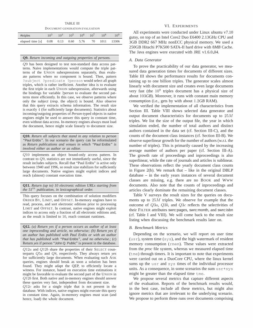
TABLE III

DOCUMENT GENERATION EVALUATION

#triples 103

104

105

106

107

108

109

elapsed time [s] 0.08 0.13 0.60 5.76 70 1011 13306

Q9. Return incoming and outgoing properties of persons.

Q9 has been designed to test non-standard data access pat-terns. Naive implementations would compute the triple pat-terns of the UNION subexpressions separately, thus evalu-ate patterns where no component is bound. Then, pattern?subject ?predicate ?person would select all graphtriples, which is rather inefficient. Another idea is to evaluatethe first triple in each UNION subexpression, afterwards usingthe bindings for variable?personto evaluate the second pat-terns more efficiently. In this case, we observe patterns whereonly the subject (resp. theobject) is bound. Also observethat this query extracts schema information. The result sizeis exactly4 (for sufficiently large documents). Statistics aboutincoming/outgoing properties ofPerson-typed objects in nativeengines might be used to answer this query in constant time,even without data access. In-memory engines always must loadthe document, hence might scale linearly to document size.

Q10. Return all subjects that stand in any relation to person“ Paul Erdos”. In our scenario the query can be reformulatedas Return publications and venues in which “Paul Erdos” isinvolved either as author or as editor.

Q10 implements an object bound-only access pattern. Incontrast toQ9, statistics are not immediately useful, since theresult includes subjects. Recall that “Paul Erdos” is active onlybetween 1940 and 1996, so result size stabilizes for sufficientlylarge documents. Native engines might exploit indices andreach (almost) constant execution time.

Q11. Return (up to) 10 electronic edition URLs starting fromthe 51th publication, in lexicographical order.

This query focuses on the combination of solution modifiersORDERBY, L IMIT , and OFFSET. In-memory engines have toread, process, and sort electronic editions prior to processingL IMIT and OFFSET. In contrast, native engines might exploitindices to access only a fraction of all electronic editionsand,as the result is limited to10, reach constant runtimes.

Q12. (a) Return yes if a person occurs as author of at leastone inproceeding and article, no otherwise; (b) Return yes ifan author has published with Paul Erdos or with an authorthat has published with “Paul Erdos”, and no otherwise.; (c)Returnyesif person “John Q. Public” is present in the database.

Q12a and Q12b share the properties of their SELECT coun-terpartsQ5a and Q8, respectively. They always returnyesfor sufficiently large documents. When evaluating such ASKqueries, engines should break as soon a solution has beenfound. They might adapt the QEP, to efficiently locate awitness. For instance, based on execution time estimationsitmight be favorable to evaluate the second part of the UNION inQ12b first. Both native and in-memory engines should answerthese queries very fast, independent from document size.Q12c asks for a single triple that is not present in thedatabase. With indices, native engines might execute this queryin constant time. Again, in-memory engines must scan (andhence, load) the whole document.

VI. EXPERIMENTS

All experiments were conducted under Linux ubuntu v7.10gutsy, on top of an Intel Core2 Duo E6400 2.13GHz CPU and3GB DDR2 667 MHz nonECC physical memory. We used a250GB Hitachi P7K500 SATA-II hard drive with 8MB Cache.The Java engines were executed with JRE v1.6.004.

A. Data Generator

To prove the practicability of our data generator, we mea-sured data generation times for documents of different sizes.Table III shows the performance results for documents con-taining up to one billion triples. The generator scales almostlinearly with document size and creates even large documentsvery fast (the109 triples document has a physical size ofabout103GB). Moreover, it runs with constant main memoryconsumption (i.e., gets by with about1.2GB RAM).

We verified the implementation of all characteristics fromSection III. Table VIII shows selected data generator andoutput document characteristics for documents up to25M

triples. We list the size of the output file, the year in whichsimulation ended, the number of total authors and distinctauthors contained in the data set (cf. Section III-C), and thecounts of the document class instances (cf. Section III-B).Weobserve superlinear growth for the number of authors (w.r.t. thenumber of triples). This is primarily caused by the increasingaverage number of authors per paper (cf. Section III-A).The growth rate of proceedings and inproceedings is alsosuperlinear, while the rate of journals and articles is sublinear.These observations reflect the yearly document class countsin Figure 2(b). We remark that – like in the original DBLPdatabase – in the early years instances of several documentclasses are missing, e.g. there are no BOOK and WWW

documents. Also note that the counts of inproceedings andarticles clearly dominate the remaining document classes.

Table V surveys the result sizes for the queries on docu-ments up to25M triples. We observe for example that theoutcome ofQ3a, Q3b, and Q3c reflects the selectivities oftheir FILTER attributesswrc:pages, swrc:month, andswrc:isbn(cf. Table I and VIII). We will come back to the result sizelisting when discussing the benchmark results later on.

B. Benchmark Metrics

Depending on the scenario, we will report on user time(usr ), system time (sys ), and the high watermark of residentmemory consumption (rmem). These values were extractedfrom theproc file system, whereas we measured elapsed time(tme ) through timers. It is important to note that experimentswere carried out on a DuoCore CPU, where the linux kernelsums up theusr and sys times of the individual processorunits. As a consequence, in some scenarios the sumusr +sysmight be greater than the elapsed timetme .

We propose several metrics that capture different aspectsof the evaluation. Reports of the benchmark results would,in the best case, include all these metrics, but might alsoignore metrics that are irrelevant to the underlying scenario.We propose to perform three runs over documents comprising

10k, 50k, 250k, 1M , 5M , and 25M triples, using a fixedtimeout of 30min per query and document, always reportingon the average value over all three runs and, if significant, theerrors within these runs. We point out that this setting can beevaluated in reasonable time (typically within few days). Ifthe implementation is fast enough, nothing prevents the userfrom adding larger documents. All reports should, of course,include the hardware and software specifications. Performanceresults should listtme , and optionallyusr and sys . In thefollowing, we shortly describe a set of interesting metrics.

1) SUCCESS RATE: We propose to separately report onthe success rates for the engine on top of all documentsizes, distinguishing betweenSuccess, Timeout (e.g. anexecution time> 30min as used in our experimentshere), Memory Exhaustion (if an additional memorylimit was set), and generalErrors. This metric gives agood survey over scaling properties and might give firstinsights into the behavior of engines.

2) LOADING TIME: The user should report on the loadingtimes for the documents of different sizes. This metricprimarily applies to engines with a database backend andmight be ignored for in-memory engines, where loadingis typically part of the evaluation process.

3) PER-QUERY PERFORMANCE: The report should includethe individual performance results for all queries over alldocument sizes. This metric is more detailed than theSUCCESSRATE report and forms the basis for a deepstudy of the results, in order to identify strengths andweaknesses of the tested implementation.

4) GLOBAL PERFORMANCE: We propose to combine theper-query results into a single performance measure.Here we recommend to list for execution times thearithmetic as well as the geometric mean, which isdefined as the nth root of the product overn numbers.In the context of SP2Bench, this means we multiplythe execution time of all17 queries (queries that failedshould be ranked with3600s, to penalize timeouts andother errors) and compute the 17th root of this product(for each document size, accordingly). This metric iswell-suited to compare the performance of engines.

5) MEMORY CONSUMPTION: In particular for engines witha physical backend, the user should also report onthe high watermark of main memory consumption andideally also the average memory consumption over allqueries (cf. Table VI and VII).

C. Benchmark Results for Selected Engines

It is beyond the scope of this paper to provide an in-depthcomparison of existing SPARQL engines. Rather than that,we use our metrics to give first insights into the state-of-theart and exemplarily illustrate that the benchmark indeed givesvaluable hints on bottlenecks in current implementations.Inthis line, we are not primarily interested in concrete values(which, however, might be of great interest in the generalcase), but focus on the principal behavior and properties ofengines, e.g. discuss how they scale with document size. We

will exemplarily discuss some interesting cases and refer theinterested reader to the Appendix for the complete results.

We conducted benchmarks for (1) the Java engineARQ13

v2.2 on top of Jena 2.5.5, (2) theRedland14 RDF Proces-sor v1.0.7 (written in C), using the Raptor Parser Toolkitv.1.4.16 and Rasqal Library v0.9.15, (3)SDB15, which linkARQ to an SQL database back-end (i.e., we used mysqlv5.0.34) , (4) the Java implementationSesame16 v2.2beta2,and finally (5) OpenLinkVirtuoso17 v5.0.6 (written in C).

For Sesame we tested two configurations:SesameM , whichprocesses queries in memory, andSesameDB, which storesdata physically on disk, using the nativeMulgara SAIL(v1.3beta1). We thus distinguish between the in-memory en-gines (ARQ, SesameM ) and engines with physical backend,namely (Redland, SBD, SesameDB, Virtuoso). The latter canfurther be divided into engines with a native RDF store (Red-land, SesameDB, Virtuoso) and a relational database backend(SDB). For all physical-backend databases we created indiceswherever possible (immediately after loading the documents)and consider loading and execution time separately (indexcreation time is included in the reported loading times).

We performed three cold runs over all queries and docu-ments of10k, 50k, 250k, 1M , 5M , and25M triples, i.e. in-between each two runs we restarted the engines and clearedthe database. We set a timeout of30min (tme ) per query anda memory limit of2.6GB, either usingulimit or restricting theJVM (for higher limits, the initialization of the JVM failed).Negative and positive variation of the average (over the runs)was < 2% in almost all cases, so we omit error bars. ForSDB and Virtuoso, which follow a client-server architecture,we monitored both processes and sum up these values.

We verified all results by comparing the outputs, observingthat SDB and Redlandreturned wrong results for a coupleof queries, so we restrict ourselves on the discussion of theremaining four engines. Table IV shows the success rates.All queries that are not listed succeeded, except forARQand SesameM on the25M document (either due to timeoutor memory exhaustion) and Virtuoso onQ6 (due to missingstandard compliance). Hence,Q4, Q5a, Q6, andQ7 are themost challenging queries, where we observe many timeoutseven for small documents. Note that we did not succeed inloading the25M triples document into theVirtuosodatabase.

D. Discussion of Benchmark Results

Main Memory. For the in-memory engines we observethat the high watermark of main memory consumption dur-ing query evaluation increases sublinearly to document size(cf. Table VI), e.g. for ARQ we measured an average (overruns and queries) of85MB on 10k, 166MB on 50k, 318MB on250k, 526MB on 1M , and1.3GB on 5M triples. Somewhat

13http://jena.sourceforge.net/ARQ/14http://librdf.org/15http://jena.sourceforge.net/SDB/16http://www.openrdf.org/17http://www.openlinksw.com/virtuoso/

TABLE IV

SUCCESS RATES FOR QUERIES ONRDF DOCUMENTS UP TO25M TRIPLES. QUERIES ARE ENCODED IN HEXADECIMAL(E.G., ’A’ STANDS FORQ10). WE

USE THE SHORTCUTS+:=SUCCESS, T:=TIMEOUT, M:=MEMORY EXHAUSTION, AND E:=ERROR.

ARQ SesameM SesameDB Virtuoso

Query 123 45 6789ABC 123 45 6789ABC 123 45 6789ABC 123 45 6789ABCabc ab abc ab abc ab abc ab

10k +++++++++++++++++ +++++++++++++++++ +++++++++++++++++ ++++++++E++++++++50k +++++++++++++++++ +++++++++++++++++ +++++++++++++++++ ++++++++E++++++++250k +++++T+++++++++++ ++++++T+T++++++++ ++++++T+TT+++++++ +++++TT+E++++++++1M +++++TT+TT+++++++ ++++++T+TT+++++++ ++++++T+TT+++++++ +++++TTTET+++++++5M +++++TT+TT+++++++ +++++TT+TT+++++++ +++++MT+TT+++++++ +++++TTTET+++++++25M TTTTTTTTTTTTTTTTT MMMMMMMTMMMMMTMMT +++++TT+TT+++++++(loading of document failed)

TABLE V

NUMBER OF QUERY RESULTS ON DOCUMENTS UP TO25 MILLION TRIPLES

Query Q1 Q2 Q3a Q3b Q3c Q4 Q5a Q5b Q6 Q7 Q8 Q9 Q10 Q11

10k 1 147 846 9 0 23226 155 155 229 0 184 4 166 1050k 1 965 3647 25 0 104746 1085 1085 1769 2 264 4 307 10250k 1 6197 15853 127 0 542801 6904 6904 12093 62 332 4 452 101M 1 32770 52676 379 0 2586733 35241 35241 62795 292 400 4 572 105M 1 248738 192373 1317 0 18362955 210662 210662 417625 1200 4934 656 1025M 1 1876999 594890 4075 0 n/a 696681 696681 1945167 5099 493 4 656 10

TABLE VI

ARITHMETIC AND GEOMETRIC MEANS OF EXECUTION TIME(Ta /Tg ) AND

ARITHMETIC MEAN OF MEMORY CONSUMPTION(Ma) FOR THE

IN-MEMORY ENGINES

ARQ SesameM

Ta[s] Tg [s] Ma[MB] Ta[s] Tg [s] Ma[MB]

250k 491.87 56.35 318.25 442.47 28.64 272.271M 901.73 179.42 525.61 683.16 106.38 561.795M 1154.80 671.41 1347.55 1059.03 506.14 1437.38

surprisingly, also the memory consumption of the nativeenginesVirtuosoandSesameDB increased with document size.

Arithmetic and Geometric Mean. For the in-memory en-gines we observe thatSesameM is superior toARQ regardingboth means (see Table VI). For instance, the arithmetic (Ta)and geometric (Tg) mean for the engines on the1M documentover all queries18 areT SesM

a = 683.16s, T SesMg = 106.84s,

T ARQa = 901.73s, andT ARQ

g = 179.42s.For the native engines on1M triples (cf. Table VII) we have

T SesDBa = 653.17s, T SesDB

g = 10.17s, T V irta = 850.06s,

and T V irtg = 3.03s. The arithmetic mean ofSesameDB is

superior, which is mainly due to the fact that it failed only on4 (vs. 5) queries. The geometric mean moderates the impactof these outliers.Virtuososhows a better overall performancefor the success queries, so its geometric mean is superior.

In-memory Engines. Figure 5 (top) plot selected resultsfor in-memory engines. We start withQ5a andQ5b. Althoughboth compute the same result, the engines perform much betterfor the explicit join inQ5b. We may suspect that the implicitjoin in Q5a is not recognized, i.e. that both engines compute

18We always penalize failure queries with3600s.

TABLE VII

ARITHMETIC AND GEOMETRIC MEANS OF EXECUTION TIME(Ta /Tg ) AND

ARITHMETIC MEAN OF MEMORY CONSUMPTION(Ma) FOR THE NATIVE

ENGINES

SesameDB Virtuoso

Ta[s] Tg [s] Ma[MB] Ta[s] Tg [s] Ma[MB]

250k 639.86 6.79 73.92 546.31 1.31 377.601M 653.17 10.17 145.97 850.06 3.03 888.725M 860.33 22.91 196.33 870.16 8.96 1072.84

the cartesian product and apply the filter afterwards.Q6 and Q7 implement simple and double negation, re-

spectively. Both engines show insufficient behavior. At thefirst glance, we might expect thatQ7 (which involves doublenegation) is more complicated to evaluate, but we observethat SesameM scales even worse forQ6. We identify twopossible explanations. First,Q7 “negates” documents withincoming citations, but – according to Section III-D – onlya small fraction of papers has incoming citations at all. Incontrast,Q6 negates arbitrary documents, i.e. a much largerset. Another reasonable cause might be the non-equality filtersubexpression?yr2 < ?yr inside the inner FILTER of Q6.

For ASK query Q12a both engines scale linearly withdocument size. However, from Table V and the fact that ourdata generator is incremental and deterministic, we know thata “witness” is already contained in the first10k triples of thedocument. It might be located even without reading the wholedocument, so both evaluation strategies are suboptimal.

Native Engines.The leftmost plot at the bottom of Figure 5shows the loading times for the native enginesSesameDB andVirtuoso. Both engines scale well concerningusr and sys ,essentially linear to document size. ForSesameDB, however,

0.001

0.01

0.1

1

10

100

1000

10000

S1 S2 S3 S4 S5 S6 S1 S2 S3 S4 S5 S6

time

in s

econ

ds

Q5aARQ (left) vs. SesameM (right)

Fai

lure

Fai

lure

Fai

lure

Fai

lure

Fai

lure

Fai

lure

Fai

lure

usr+syssystme

0.001

0.01

0.1

1

10

100

1000

10000

S1 S2 S3 S4 S5 S6 S1 S2 S3 S4 S5 S6

Q5bARQ (left) vs. SesameM (right)

Fai

lure

Fai

lure

usr+syssystme

0.001

0.01

0.1

1

10

100

1000

10000

S1 S2 S3 S4 S5 S6 S1 S2 S3 S4 S5 S6

Q6ARQ (left) vs. SesameM (right)

Fai

lure

Fai

lure

Fai

lure

Fai

lure

Fai

lure

Fai

lure

Fai

lure

usr+syssystme

0.001

0.01

0.1

1

10

100

1000

10000

S1 S2 S3 S4 S5 S6 S1 S2 S3 S4 S5 S6

Q7ARQ (left) vs. SesameM (right)

Fai

lure

Fai

lure

Fai

lure

Fai

lure

Fai

lure

Fai

lure

usr+syssystme

0.001

0.01

0.1

1

10

100

1000

10000

S1 S2 S3 S4 S5 S6 S1 S2 S3 S4 S5 S6

Q12aARQ (left) vs. SesameM (right)

Fai

lure

Fai

lure

usr+syssystme

0.001

0.01

0.1

1

10

100

1000

10000

100000

1e+06

S1 S2 S3 S4 S5 S6 S1 S2 S3 S4 S5

time

in s

econ

ds

LoadingSesameDB (left) vs. Virtuoso (right)

usr+syssystme

0.001

0.01

0.1

1

10

100

1000

10000

S1 S2 S3 S4 S5 S6 S1 S2 S3 S4 S5

Q2SesameDB vs. Virtuoso (right)

usr+syssystme

0.001

0.01

0.1

1

10

100

1000

S1 S2 S3 S4 S5 S6 S1 S2 S3 S4 S5

Q3aSesameDB vs. Virtuoso (right)

usr+syssystme

0.001

0.01

0.1

1

10

100

S1 S2 S3 S4 S5 S6 S1 S2 S3 S4 S5

Q3cSesameDB vs. Virtuoso (right)

usr+syssystme

0.001

0.01

0.1

1

10

S1 S2 S3 S4 S5 S6 S1 S2 S3 S4 S5

Q10SesameDB vs. Virtuoso (right)

usr+syssystme

Fig. 5. Results for in-memory engines (top) and native engines (bottom) on S1=10k, S2=50k, S3=250k, S4=1M, S5=5M, and S6=25M triples

tme grows superlinearly (e.g., loading of the25M documentis about ten times slower than loading of the5M document).This might cause problems for larger documents.

The running times forQ2 increase superlinear for bothengines (in particular for larger documents). This reflectsthesuperlinear growth of inproceedings and the growing resultsize (cf. Tables VIII and V). What is interesting here is the sig-nificant difference betweenusr+sys and tme for Virtuoso,which indicates disproportional disk I/O. SinceSesamedoesnot exhibit this peculiar behavior, it might be an interestingstarting point for further optimizations in theVirtuosoengine.

QueriesQ3a andQ3c have been designed to test the intel-ligent choice of indices in the context of FILTER expressionswith varying selectivity.Virtuoso gets by with an economicconsumption ofusr and sys time for both queries, whichsuggests that it makes heavy use of indices. While this strategypays off for Q3c, the elapsed time forQ3a is unreasonablyhigh and we observe thatSesameM scales better for this query.

Q10 extracts subjects and predicates that are associated withPaul Erdos. First recall that, for each year up to1996, PaulErdos has exactly10 publications and occurs twice as editor(cf. Section IV). Both engines answer this query in aboutconstant time, which is possible due to the upper result sizebound (cf. Table V). Regardingusr+sys , Virtuoso is evenmore efficient: These times are diminishing in all cases. Hence,this query constitutes an example for desired engine behavior.

VII. C ONCLUSION

We have presented the SP2Bench performance benchmarkfor SPARQL, which constitutes the first methodical approachfor testing the performance of SPARQL engines w.r.t. differ-ent operator constellations, RDF access paths, typical RDFconstructs, and a variety of possible optimization approaches.

Our data generator relies on a deep study of DBLP. Al-though it is not possible to mirrorall correlations found in theoriginal DBLP data (e.g., we simplified when assuming inde-pendence between attributes in Section III-A), many aspects

TABLE VIII

CHARACTERISTICS OF GENERATED DOCUMENTS

#Triples 10k 50k 250k 1M 5M 25M

file size [MB] 1.0 5.1 26 106 533 2694data up to 1955 1967 1979 1989 2001 2015

#Tot.Auth. 1.5k 6.8k 34.5k 151.0k 898.0k 5.4M#Dist.Auth. 0.9k 4.1k 20.0k 82.1k 429.6k 2.1M

#Journals 25 104 439 1.4k 4.6k 11.7k#Articles 916 4.0k 17.1k 56.9k 207.8k 642.8k#Proc. 6 37 213 903 4.7k 24.4k#Inproc. 169 1.4k 9.2k 43.5k 255.2k 1.5M#Incoll. 18 56 173 442 1.4k 4.5k#Books 0 0 39 356 973 1.7k#PhD Th. 0 0 0 101 237 365#Mast.Th. 0 0 0 50 95 169#WWWs 0 0 0 35 92 168

are modeled in faithful detail and the queries are designed insuch a way that they build on exactly those aspects, whichmakes them realistic, understandable, and predictable.

Even without knowledge about the internals of engines, weidentified deficiencies and reasoned about suspected causes.We expect the benefit of our benchmark to be even higher fordevelopers that are familiar with the engine internals.

To give another proof of concept, in [33] we have suc-cessfully used SP2Bench to identify previously unknown lim-itations of RDF storage schemes: Among others, we iden-tified scenarios where the advanced vertical storage schemefrom [12] was slower than a simple triple store approach.

With the understandable DBLP scenario we clear the wayfor coming language modifications. For instance, SPARQLupdate and aggregation support are currently discussed aspossible extensions.19 Updates, for instance, could be real-ized by minor extensions to our data generator. Concerningaggregations, the detailed knowledge of the document classcounts and distributions (cf. Section III) facilitates thedesignof challenging aggregate queries with fixed characteristics.

19See http://esw.w3.org/topic/SPARQL/Extensions.

REFERENCES

[1] “Resource Description Framework (RDF): Concepts and Abstract Syn-tax,” http://www.w3.org/TR/rdf-concepts/. W3C Rec. 02/2004.

[2] T. Berners-Lee, J. Hendler, and O. Lassila, “The Semantic Web,”Scientific American, May 2001.

[3] “SPARQL Query Language for RDF,” http://www.w3.org/TR/rdf-sparql-query/. W3C Rec. 01/2008.

[4] J. Perez, M. Arenas, and C. Gutierrez, “Semantics and Complexity ofSPAQRL,” in ISWC, 2006, pp. 30–43.

[5] M. Stocker et al., “SPARQL Basic Graph Pattern Optimization UsingSelectivity Estimation,” inWWW, 2008, pp. 595–604.

[6] O. Hartwig and R. Heese, “The SPARQL Query Graph Model forQueryOptimization,” in ESWC, 2007, pp. 564–578.

[7] S. Groppe, J. Groppe, and V. Linnemann, “Using an Index ofPrecom-puted Joins in order to speed up SPARQL Processing,” inICEIS, 2007,pp. 13–20.

[8] A. Harth and S. Decker, “Optimized Index Structures for Querying RDFfrom the Web,” inLA-WEB, 2005, pp. 71–80.

[9] S. Alexaki et al., “On Storing Voluminous RDF descriptions: The caseof Web Portal Catalogs,” inWebDB, 2001.

[10] J. Broekstra, A. Kampman, and F. van Harmelen, “Sesame:A GenericArchitecture for Storing and Querying RDF and RDF Schema,” in ISWC,2002, pp. 54–68.

[11] S. Harris and N. Gibbins, “3store: Efficient Bulk RDF Storage,” inPSSS,2003.

[12] D. J. Abadi et al., “Scalable Semantic Web Data Management UsingVertical Partitioning,” inVLDB, 2007, pp. 411–422.

[13] C. Weiss, P. Karras, and A. Bernstein, “Hexastore: Sextuple Indexingfor Semantic Web Data Management,” inVLDB, 2008.

[14] G. Lausen, M. Meier, and M. Schmidt, “SPARQLing Constraints forRDF,” in EDBT, 2008, pp. 499–509.

[15] R. Cyganiac, “A relational algebra for SPARQL,” HP LaboratoriesBristol, Tech. Rep., 2005.

[16] A. Chebotko et al., “Semantics Preserving SPARQL-to-SQL QueryTranslation for Optional Graph Patterns,” TR-DB-052006-CLJF.

[17] A. Polleres, “From SPARQL to Rules (and back),” inWWW, 2007, pp.787–796.

[18] Z. P. Yuanbo Guo and J. Heflin, “LUBM: A Benchmark for OWLKnowledge Base Systems,”Web Semantics: Science, Services andAgents on the WWW, vol. 3, pp. 158–182, 2005.

[19] D. J. Abadi et al., “Using the Barton libraries dataset as an RDFbenchmark,” TR MIT-CSAIL-TR-2007-036, MIT.

[20] A. Schmidt et al., “XMark: A Benchmark for XML Data Management,”in VLDB, 2002, pp. 974–985.

[21] M. Ley, “DBLP Database,” http://www.informatik.uni-trier.de/∼ ley/db/.[22] E. Elmacioglu and D. Lee, “On Six Degrees of Separation in DBLP-DB

and More,”SIGMOD Record, vol. 34, no. 2, pp. 33–40, 2005.[23] J. Gray, The Benchmark Handbook for Database and Transaction

Systems. Morgan Kaufmann, 1993.[24] M. J. Carey, D. J. DeWitt, and J. F. Naughton, “The OO7 Benchmark,”

in SIGMOD, 1993, pp. 12–21.[25] “RDF Vocabulary Description Language 1.0: RDF Schema,”

http://www.w3.org/TR/rdf-schema/. W3C Rec. 02/2004.[26] “RDF Semantics,” http://www.w3.org/TR/rdf-mt/. W3CRec. 02/2004.[27] C. Bizer and A. Schultz, “Benchmarking the Performanceof Storage

Systems that expose SPARQL Endpoints,” inSSWS, 2008.[28] A. Magkanaraki et al., “Benchmarking RDF Schemas for the Semantic

Web,” in ISWC, 2002, p. 132.[29] Y. Theoharis et al., “On Graph Features of Semantic Web Schemas,”

IEEE Trans. Knowl. Data Eng., vol. 20, no. 5, pp. 692–702, 2008.[30] S. Wang et al., “Rapid Benchmarking for Semantic Web Knowledge

Base Systems,” inISWC, 2005, pp. 758–772.[31] C. Bizer and R. Cyganiak, “D2R Server publishing the DBLP Bibliog-

raphy Database,” 2007, http://www4.wiwiss.fu-berlin.de/dblp/.[32] A. J. Lotka, “The Frequency Distribution of Scientific Production,”

Acad. Sci., vol. 16, pp. 317–323, 1926.[33] M. Schmidt et al., “An Experimental Comparison of RDF Data Manage-

ment Approaches in a SPAQL Benchmark Scenario,” inISWC, 2008.

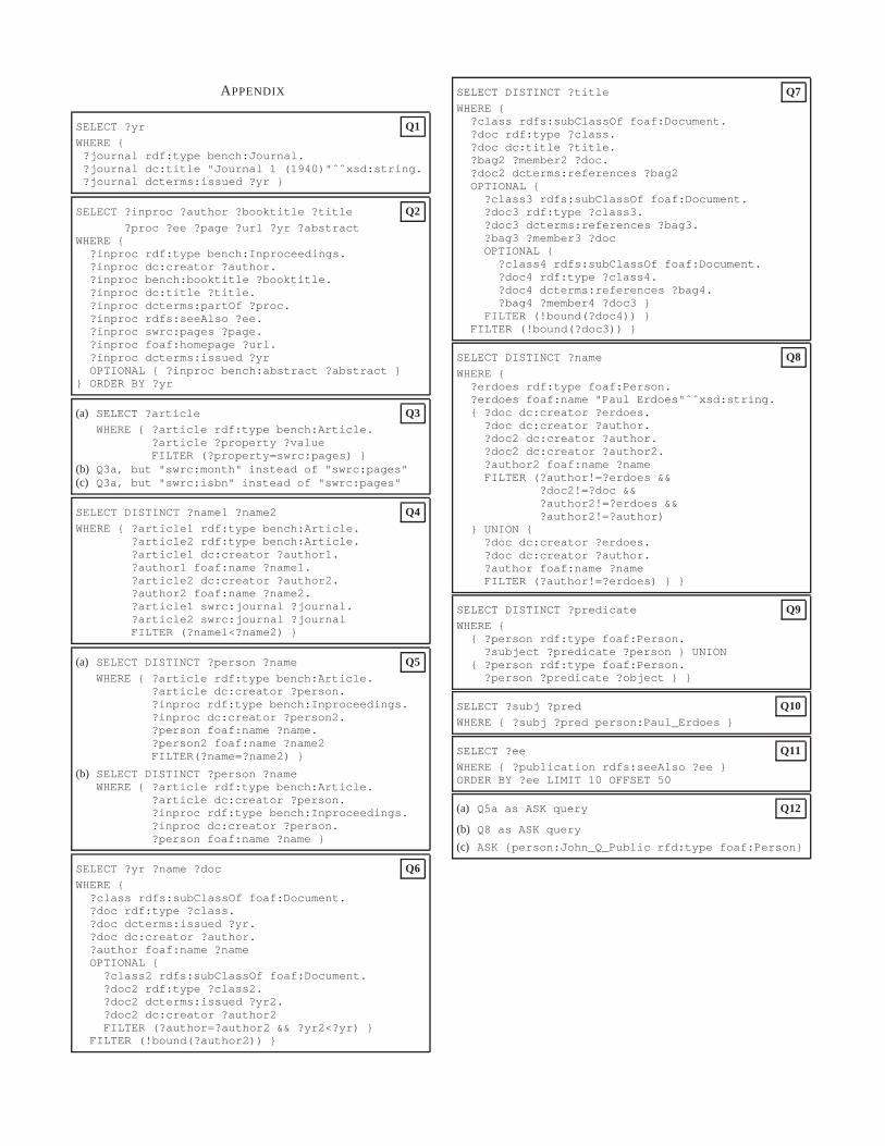
APPENDIX

SELECT ?yr Q1WHERE {

?journal rdf:type bench:Journal.?journal dc:title "Journal 1 (1940)"ˆˆxsd:string.?journal dcterms:issued ?yr }

SELECT ?inproc ?author ?booktitle ?title Q2?proc ?ee ?page ?url ?yr ?abstract

WHERE {?inproc rdf:type bench:Inproceedings.?inproc dc:creator ?author.?inproc bench:booktitle ?booktitle.?inproc dc:title ?title.?inproc dcterms:partOf ?proc.?inproc rdfs:seeAlso ?ee.?inproc swrc:pages ?page.?inproc foaf:homepage ?url.?inproc dcterms:issued ?yrOPTIONAL { ?inproc bench:abstract ?abstract }

} ORDER BY ?yr

(a) SELECT ?article Q3WHERE { ?article rdf:type bench:Article.

?article ?property ?valueFILTER (?property=swrc:pages) }

(b) Q3a, but "swrc:month" instead of "swrc:pages"(c) Q3a, but "swrc:isbn" instead of "swrc:pages"

SELECT DISTINCT ?name1 ?name2 Q4WHERE { ?article1 rdf:type bench:Article.

?article2 rdf:type bench:Article.?article1 dc:creator ?author1.?author1 foaf:name ?name1.?article2 dc:creator ?author2.?author2 foaf:name ?name2.?article1 swrc:journal ?journal.?article2 swrc:journal ?journalFILTER (?name1<?name2) }

(a) SELECT DISTINCT ?person ?name Q5WHERE { ?article rdf:type bench:Article.

?article dc:creator ?person.?inproc rdf:type bench:Inproceedings.?inproc dc:creator ?person2.?person foaf:name ?name.?person2 foaf:name ?name2FILTER(?name=?name2) }

(b) SELECT DISTINCT ?person ?nameWHERE { ?article rdf:type bench:Article.

?article dc:creator ?person.?inproc rdf:type bench:Inproceedings.?inproc dc:creator ?person.?person foaf:name ?name }

SELECT ?yr ?name ?doc Q6WHERE {

?class rdfs:subClassOf foaf:Document.?doc rdf:type ?class.?doc dcterms:issued ?yr.?doc dc:creator ?author.?author foaf:name ?nameOPTIONAL {

?class2 rdfs:subClassOf foaf:Document.?doc2 rdf:type ?class2.?doc2 dcterms:issued ?yr2.?doc2 dc:creator ?author2FILTER (?author=?author2 && ?yr2<?yr) }

FILTER (!bound(?author2)) }

SELECT DISTINCT ?title Q7WHERE {

?class rdfs:subClassOf foaf:Document.?doc rdf:type ?class.?doc dc:title ?title.?bag2 ?member2 ?doc.?doc2 dcterms:references ?bag2OPTIONAL {

?class3 rdfs:subClassOf foaf:Document.?doc3 rdf:type ?class3.?doc3 dcterms:references ?bag3.?bag3 ?member3 ?docOPTIONAL {

?class4 rdfs:subClassOf foaf:Document.?doc4 rdf:type ?class4.?doc4 dcterms:references ?bag4.?bag4 ?member4 ?doc3 }

FILTER (!bound(?doc4)) }FILTER (!bound(?doc3)) }

SELECT DISTINCT ?name Q8WHERE {

?erdoes rdf:type foaf:Person.?erdoes foaf:name "Paul Erdoes"ˆˆxsd:string.{ ?doc dc:creator ?erdoes.

?doc dc:creator ?author.?doc2 dc:creator ?author.?doc2 dc:creator ?author2.?author2 foaf:name ?nameFILTER (?author!=?erdoes &&

?doc2!=?doc &&?author2!=?erdoes &&?author2!=?author)

} UNION {?doc dc:creator ?erdoes.?doc dc:creator ?author.?author foaf:name ?nameFILTER (?author!=?erdoes) } }

SELECT DISTINCT ?predicate Q9WHERE {

{ ?person rdf:type foaf:Person.?subject ?predicate ?person } UNION

{ ?person rdf:type foaf:Person.?person ?predicate ?object } }

SELECT ?subj ?pred Q10WHERE { ?subj ?pred person:Paul_Erdoes }

SELECT ?ee Q11WHERE { ?publication rdfs:seeAlso ?ee }ORDER BY ?ee LIMIT 10 OFFSET 50

(a) Q5a as ASK query Q12

(b) Q8 as ASK query

(c) ASK {person:John_Q_Public rfd:type foaf:Person}

0.001

0.01

0.1

1

10

100

1000

S1 S2 S3 S4 S5 S6

Q1 - ARQ

Fai

lure

usr+syssystme

0.001

0.01

0.1

1

10

100

1000

S1 S2 S3 S4 S5 S6

Q1 - SesameM

Fai

lure

usr+syssystme

0.001

0.01

0.1

1

10

100

S1 S2 S3 S4 S5 S6

Q1 - SesameDB

usr+syssystme

0.001

0.01

0.1

1

10

S1 S2 S3 S4 S5

Q1 - Virtuosousr+sys

systme

0.001

0.01

0.1

1

10

100

1000

10000

S1 S2 S3 S4 S5 S6

Q2 - ARQ

Fai

lure

usr+syssystme

0.001

0.01

0.1

1

10

100

1000

S1 S2 S3 S4 S5 S6

Q2 - SesameM

Fai

lure

usr+syssystme

0.001

0.01

0.1

1

10

100

1000

10000

S1 S2 S3 S4 S5 S6

Q2 - SesameDBusr+sys

systme

0.001

0.01

0.1

1

10

100

1000

S1 S2 S3 S4 S5

Q2 - Virtuosousr+sys

systme

0.001

0.01

0.1

1

10

100

1000

S1 S2 S3 S4 S5 S6

Q3a - ARQ

Fai

lure

usr+syssystme

0.001

0.01

0.1

1

10

100

1000

S1 S2 S3 S4 S5 S6

Q3a - SesameM

Fai

lure

usr+syssystme

0.001

0.01

0.1

1

10

100

1000

S1 S2 S3 S4 S5 S6

Q3a - SesameDBusr+sys

systme

0.001

0.01

0.1

1

10

100

1000

S1 S2 S3 S4 S5

Q3a - Virtuosousr+sys

systme

0.001

0.01

0.1

1

10

100

1000

S1 S2 S3 S4 S5 S6

Q3b - ARQ

Fai

lure

usr+syssystme

0.001

0.01

0.1

1

10

100

1000

S1 S2 S3 S4 S5 S6

Q3b - SesameM

Fai

lure

usr+syssystme

0.001

0.01

0.1

1

10

100

S1 S2 S3 S4 S5 S6

Q3b - SesameDB

usr+syssystme

0.001

0.01

0.1

1

10

S1 S2 S3 S4 S5

Q3b - Virtuosousr+sys

systme

0.001

0.01

0.1

1

10

100

1000

S1 S2 S3 S4 S5 S6

Q3c - ARQ

Fai

lure

usr+syssystme

0.001

0.01

0.1

1

10

100

1000

S1 S2 S3 S4 S5 S6

Q3c - SesameM

Fai

lure

usr+syssystme

0.001

0.01

0.1

1

10

100

S1 S2 S3 S4 S5 S6

Q3c - SesameDB

usr+syssystme

0.001

0.01

0.1

1

10

S1 S2 S3 S4 S5

Q3c - Virtuosousr+sys

systme

0.001

0.01

0.1

1

10

100

1000

S1 S2 S3 S4 S5 S6

Q4 - ARQ

Fai

lure

Fai

lure

Fai

lure

Fai

lure

usr+syssystme

0.001

0.01

0.1

1

10

100

1000

S1 S2 S3 S4 S5 S6

Q4 - SesameM

Fai

lure

Fai

lure

usr+syssystme

0.001

0.01

0.1

1

10

100

1000

S1 S2 S3 S4 S5 S6

Q4 - SesameDB

Fai

lure

Fai

lure

usr+syssystme

0.001

0.01

0.1

1

10

100

1000

S1 S2 S3 S4 S5

Q4 - Virtuoso

Fai

lure

Fai

lure

Fai

lure

usr+syssystme

Fig. 6. Query evaluation results on S1=10k, S2=50k, S3=250k, S4=1M, S5=5M, and S6=25M triples

0.001

0.01

0.1

1

10

100

1000

10000

S1 S2 S3 S4 S5 S6

Q5a - ARQ

Fai

lure

Fai

lure

Fai

lure

usr+syssystme

0.001

0.01

0.1

1

10

100

1000

S1 S2 S3 S4 S5 S6

Q5a - SesameM

Fai

lure

Fai

lure

Fai

lure

Fai

lure

usr+syssystme

0.001

0.01

0.1

1

10

100

1000

S1 S2 S3 S4 S5 S6

Q5a - SesameDB

Fai

lure

Fai

lure

Fai

lure

Fai

lure

usr+syssystme

0.001

0.01

0.1

1

10

100

1000

S1 S2 S3 S4 S5

Q5a - Virtuoso

Fai

lure

Fai

lure

Fai

lure

usr+syssystme

0.001

0.01

0.1

1

10

100

1000

S1 S2 S3 S4 S5 S6

Q5b - ARQ

Fai

lure

usr+syssystme

0.001

0.01

0.1

1

10

100

1000

S1 S2 S3 S4 S5 S6

Q5b - SesameM

Fai

lure

usr+syssystme

0.001

0.01

0.1

1

10

100

1000

S1 S2 S3 S4 S5 S6

Q5b - SesameDBusr+sys

systme

0.001

0.01

0.1

1

10

100

1000

10000

S1 S2 S3 S4 S5

Q5b - Virtuoso

Fai

lure

Fai

lure

usr+syssystme

0.001

0.01

0.1

1

10

100

1000

10000

S1 S2 S3 S4 S5 S6

Q6 - ARQ

Fai

lure

Fai

lure

Fai

lure

usr+syssystme

0.001

0.01

0.1

1

10

100

1000

S1 S2 S3 S4 S5 S6

Q6 - SesameM

Fai

lure

Fai

lure

Fai

lure

Fai

lure

usr+syssystme

0.001

0.01

0.1

1

10

100

1000

S1 S2 S3 S4 S5 S6

Q6 - SesameDB

Fai

lure

Fai

lure

Fai

lure

Fai

lure

usr+syssystme

(query failed)

0.001

0.01

0.1

1

10

100

1000

10000

S1 S2 S3 S4 S5 S6

Q7 - ARQ

Fai

lure

Fai

lure

Fai

lure

usr+syssystme

0.001

0.01

0.1

1

10

100

1000

S1 S2 S3 S4 S5 S6

Q7 - SesameM

Fai

lure

Fai

lure

Fai

lure

usr+syssystme

0.001

0.01

0.1

1

10

100

1000

S1 S2 S3 S4 S5 S6

Q7 - SesameDB

Fai

lure

Fai

lure

Fai

lure

Fai

lure

usr+syssystme

0.001

0.01

0.1

1

10

100

1000

10000

S1 S2 S3 S4 S5

Q7 - Virtuoso

Fai

lure

Fai

lure

usr+syssystme

0.001

0.01

0.1

1

10

100

1000

S1 S2 S3 S4 S5 S6

Q8 - ARQ

Fai

lure

usr+syssystme

0.001

0.01

0.1

1

10

100

1000

S1 S2 S3 S4 S5 S6

Q8 - SesameM

Fai

lure

usr+syssystme

0.001

0.01

0.1

1

10

100

1000

S1 S2 S3 S4 S5 S6

Q8 - SesameDBusr+sys

systme

0.001

0.01

0.1

1

10

S1 S2 S3 S4 S5

Q8 - Virtuosousr+sys

systme

0.001

0.01

0.1

1

10

100

1000

S1 S2 S3 S4 S5 S6

Q9 - ARQ

Fai

lure

usr+syssystme

0.001

0.01

0.1

1

10

100

1000

S1 S2 S3 S4 S5 S6

Q9 - SesameM

Fai

lure

usr+syssystme

0.001

0.01

0.1

1

10

100

1000

S1 S2 S3 S4 S5 S6

Q9 - SesameDBusr+sys

systme

0.001

0.01

0.1

1

10

100

S1 S2 S3 S4 S5

Q9 - Virtuosousr+sys

systme

Fig. 7. Query evaluation results on S1=10k, S2=50k, S3=250k, S4=1M, S5=5M, and S6=25M triples

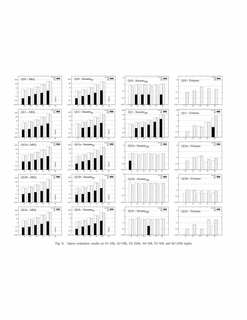
0.001

0.01

0.1

1

10

100

1000

S1 S2 S3 S4 S5 S6

Q10 - ARQ

Fai

lure

usr+syssystme

0.001

0.01

0.1

1

10

100

1000

S1 S2 S3 S4 S5 S6

Q10 - SesameM

Fai

lure

usr+syssystme

0.001

0.01

0.1

1

10

S1 S2 S3 S4 S5 S6

Q10 - SesameDB

usr+syssystme

0.001

0.01

0.1

1

10

S1 S2 S3 S4 S5

Q10 - Virtuosousr+sys

systme

0.001

0.01

0.1

1

10

100

1000

S1 S2 S3 S4 S5 S6

Q11 - ARQ

Fai

lure

usr+syssystme

0.001

0.01

0.1

1

10

100

1000

S1 S2 S3 S4 S5 S6

Q11 - SesameM

Fai

lure

usr+syssystme

0.001

0.01

0.1

1

10

100

1000

S1 S2 S3 S4 S5 S6

Q11 - SesameDBusr+sys

systme

0.001

0.01

0.1

1

10

100

S1 S2 S3 S4 S5

Q11 - Virtuosousr+sys

systme

0.001

0.01

0.1

1

10

100

1000

S1 S2 S3 S4 S5 S6

Q12a - ARQ

Fai

lure

usr+syssystme

0.001

0.01

0.1

1

10

100

1000

S1 S2 S3 S4 S5 S6

Q12a - SesameM

Fai

lure

usr+syssystme

0.001

0.01

0.1

1

10

S1 S2 S3 S4 S5 S6

Q12a - SesameDB

usr+syssystme

0.001

0.01

0.1

1

10

S1 S2 S3 S4 S5

Q12a - Virtuosousr+sys

systme

0.001

0.01

0.1

1

10

100

1000

S1 S2 S3 S4 S5 S6

Q12b - ARQ

Fai

lure

usr+syssystme

0.001

0.01

0.1

1

10

100

1000

S1 S2 S3 S4 S5 S6

Q12b - SesameM

Fai

lure

usr+syssystme

0.001

0.01

0.1

1

10

S1 S2 S3 S4 S5 S6

Q12b - SesameDB

usr+syssystme

0.001

0.01

0.1

1

10

S1 S2 S3 S4 S5

Q12b - Virtuosousr+sys

systme

0.001

0.01

0.1

1

10

100

1000

S1 S2 S3 S4 S5 S6

Q12c - ARQ

Fai

lure

usr+syssystme

0.001

0.01

0.1

1

10

100

1000

S1 S2 S3 S4 S5 S6

Q12c - SesameM

Fai

lure

usr+syssystme

0.001

0.01

0.1

1

10

S1 S2 S3 S4 S5 S6

Q12c - SesameDB

usr+syssystme

0.001

0.01

0.1

1

10

S1 S2 S3 S4 S5

Q12c - Virtuosousr+sys

systme

Fig. 8. Query evaluation results on S1=10k, S2=50k, S3=250k, S4=1M, S5=5M, and S6=25M triples

TABLE IX

PROBABILITY DISTRIBIBUTION FOR ATTRIBUTES AND DOCUMENT CLASSES

Article Inproc. Proc. Book Incoll. PhDTh. MastTh. WWW

address 0.0000 0.0000 0.0004 0.0000 0.0000 0.0000 0.0000 0.0000

author 0.9895 0.9970 0.0001 0.8937 0.8459 1.0000 1.0000 0.9973

booktitle 0.0006 1.0000 0.9579 0.0183 1.0000 0.0000 0.0000 0.0001

cdrom 0.0112 0.0162 0.0000 0.0032 0.0138 0.0000 0.0000 0.0000

chapter 0.0000 0.0000 0.0000 0.0000 0.0005 0.0000 0.0000 0.0000

cite 0.0048 0.0104 0.0001 0.0079 0.0047 0.0000 0.0000 0.0000

crossref 0.0006 0.8003 0.0016 0.0000 0.6951 0.0000 0.0000 0.0000

editor 0.0000 0.0000 0.7992 0.1040 0.0000 0.0000 0.0000 0.0004

ee 0.6781 0.6519 0.0019 0.0079 0.3610 0.1444 0.0000 0.0000

isbn 0.0000 0.0000 0.8592 0.9294 0.0073 0.0222 0.0000 0.0000

journal 0.9994 0.0000 0.0004 0.0000 0.0000 0.0000 0.0000 0.0000

month 0.0065 0.0000 0.0001 0.0008 0.0000 0.0333 0.0000 0.0000

note 0.0297 0.0000 0.0002 0.0000 0.0000 0.0000 0.0000 0.0273

number 0.9224 0.0001 0.0009 0.0000 0.0000 0.0333 0.0000 0.0000

pages 0.9261 0.9489 0.0000 0.0000 0.6849 0.0000 0.0000 0.0000

publisher 0.0006 0.0000 0.9737 0.9992 0.0237 0.0444 0.0000 0.0000

school 0.0000 0.0000 0.0000 0.0000 0.0000 1.0000 1.0000 0.0000

series 0.0000 0.0000 0.5791 0.5365 0.0000 0.0222 0.0000 0.0000

title 1.0000 1.0000 1.0000 1.0000 1.0000 1.0000 1.0000 1.0000

url 0.9986 1.0000 0.986 0.2373 0.9992 0.0222 0.3750 0.9624

volume 0.9982 0.0000 0.567 0.5024 0.0000 0.0111 0.0000 0.0000

year 1.0000 1.0000 1.0000 1.0000 1.0000 1.0000 1.0000 0.0011