Southern hemisphere sea-surface temperatures and their contemporary and lag association with New...

INTERNATIONAL JOURNAL OF CLIMATOLOGY

Int. J. Climatol. 18: 817–840 (1998)

SOUTHERN HEMISPHERE SEA-SURFACE TEMPERATURES ANDTHEIR CONTEMPORARY AND LAG ASSOCIATION WITH NEW

ZEALAND TEMPERATURE AND PRECIPITATIONA.B. MULLAN*

National Institute of Water and Atmospheric Research, Wellington, New Zealand

Recei6ed 14 March 1997Re6ised 26 September 1997

Accepted 30 September 1997

ABSTRACT

The influence of sea-surface temperature (SST) anomalies on New Zealand climate variations is examined systemat-ically, using data for the period 1949–1991. New Zealand temperature and precipitation anomalies, both monthly andseasonal, are represented in terms of rotated EOF patterns, the time series of which are then cross-correlated againstsea-surface temperature data for an extensive region of the Southern Hemisphere. Relationships with mean sea levelpressure anomalies in the Australasian region are examined to clarify significant associations found.

Monthly lead and lag cross-correlations suggest that sea temperatures in the immediate vicinity of New Zealand areresponding to atmospheric circulation variations, a result that is consistent with many similar studies elsewhereregarding midlatitude sea temperature anomalies. New Zealand temperatures, particularly in the North Island, arealso significantly correlated to the previous month’s sea-surface temperature anomaly in the western Tasman Sea andsouth of Australia, but only in autumn months (March, April, May). Subsequent analysis suggests the most likelycause of this is atmospheric forcing in the antecedent month.

On the seasonal time scale, a number of SST–New Zealand climate lag relationships are found, many of whichappear to be related to ENSO variations. However, tropical Indian Ocean SSTs unrelated to ENSO are prominentin the autumn–winter period. One phase of this teleconnection pattern is for warmer Indian Ocean waters in autumnto be followed by a stronger subtropical ridge just north of North Island in winter, stronger westerly flow over thecountry, higher South Island temperatures, more rainfall in west South Island districts and drier conditions in otherareas of the country exposed to the north and east. © 1998 Royal Meteorological Society.

KEY WORDS: New Zealand; Southern Hemisphere; climate anomalies; ENSO; sea-surface temperature; air–sea interaction; tele-connections; prewhitening; New Zealand monthly temperature; New Zealand monthly rainfall; empirical orthogonalfunction (EOF) analysis; cross-correlation; Australasian sea level pressure

1. INTRODUCTION

New Zealand is 1600 km long, but no more than 450 km wide at its widest part, and is surrounded bya large expanse of ocean. The nearest large land mass is Australia, some 1600 km to the west (NewZealand Official Yearbook, 1994). Hence, New Zealand experiences a marine climate, with minimalcontinental influence except in central South Island locations sheltered from the prevailing midlatitudewesterlies. Although subject mainly to a succession of cyclones and anticyclones in the westerlies, there isconsiderable variability in the short-term climate, and northern New Zealand can also experiencesubtropical air masses from the southwest Pacific. The influence of sea-surface temperature (SST)anomalies on New Zealand climate is therefore of considerable relevance, but the previous lack ofextensive, quality controlled, SST data has limited the number of studies that have been made.

* Correspondence to: NIWA, PO Box 14-901, Kilbirnie, Wellington, New Zealand. E-mail: [email protected]

Contract grant sponsor: New Zealand Foundation for Research, Science and Technology; Contract grant number: Contract C01522

CCC 0899–8418/98/080817–24$17.50© 1998 Royal Meteorological Society

A.B. MULLAN818

Trenberth (1975) examined monthly anomalies in mean sea level pressure (MSLP) in the Australasianregion, looking for relationships with sea-surface temperatures in the Tasman Sea (which separatesAustralia and New Zealand). A cross-spectral analysis was performed between the time series of theunrotated empirical orthogonal functions (EOFs) of the MSLP and SST anomalies, with the emphasisbeing placed on a quasi-biennial periodicity in the series. From physical and statistical considerations,Trenberth (1975) argued that SST anomalies were due largely to anomalous advection and sensible heatexchanges associated with the MSLP pattern.

Recent analyses have been carried out by Basher and Thompson (1996) and Folland and Salinger(1995). Basher and Thompson (1996) applied a co-spectral analysis to high-pass filtered series of NewZealand national-mean air temperature and area averaged SST, finding that land air temperaturesappeared to lead sea temperatures around New Zealand by about half a month. Folland and Salinger(1995) were mainly concerned with verifying the accuracy of the UK Meteorological Office monthlysea-surface temperature data set in the New Zealand region, but they did comment that on an annualtimescale, the best correlation between SST and New Zealand temperatures occurred when SST lagged thetemperatures by 1 month. These results, that suggest that SST is forced by anomalies in air temperature,which in turn are forced mainly by changes in atmospheric circulation, are consistent with the earlierfindings of Trenberth (1975).

In fact, the finding of circulation anomalies leading SST anomalies is an almost universal result for theextratropics. One of the earliest papers to report this result was Davis (1976) for the North Pacific Ocean,who found that high correlations exist between SST anomalies and MSLP anomalies when SST lagsMSLP by 1 month, but low correlations occur when the SST leads. There have been many subsequentstudies in the Northern Hemisphere that have reached similar conclusions (e.g. Lanzante, 1984; Lukschand von Storch, 1992). For the Australasian region, Whetton (1990a) and Drosdowsky (1993a) also foundthat midlatitude SST anomalies were related to the previous anomalous pressure distribution, with littleevidence of the reverse. Whetton (1990b) concluded that midlatitude Australian region SSTs did not haveany direct effect on rainfall in Victoria, Australia. All the above studies relate to climate forcing byinteractions with local SST anomalies.

The general conclusion from a large number of observational and modelling studies of air–seainteraction over the last 20 years is that equatorial SST anomalies have a pronounced effect on theatmosphere, both locally and remotely, whereas midlatitude SST anomalies produce an atmosphericresponse that is much smaller, less systematic, and likely to be seasonally dependent (Haney, 1979;Webster, 1981; Frankignoul, 1985; Graham et al., 1994).

Forcing of New Zealand climate variations by tropical SSTs, as identified with the El Nino–SouthernOscillation (ENSO), has been suggested by a number of observational studies (Gordon, 1985, 1986;Mullan, 1995, 1996). These studies have tended to use the Southern Oscillation Index (SOI) rather thansea temperatures directly. In general, during El Ninos New Zealand experiences lower temperatures, withmore rain in the south and west and less in the north and east of the country. The explained variancebetween the SOI and New Zealand rainfall and temperatures is not as great as found in other locationscloser to the centres of action, such as Australia. Spring is the season when the strongest (contemporary)linear correlations occur, and these are predominantly in the North Island, for both rainfall andtemperature. Temperature fluctuations associated with the SOI are also confined mainly to the NorthIsland again in winter, and to western areas of both islands in summer and autumn. For rainfall, thegeographic distribution of significant linear correlations is more patchy outside the spring season(Gordon, 1986).

Recent work suggests that the low-latitude Indian Ocean is also a region where sea temperatureinfluences on New Zealand climate should be sought. Nicholls (1989) found two independent patterns ofvariation of Australian rainfall, which were associated with separate specific SST patterns, as indicated bycontemporary correlations. One pattern was associated with SSTs in the central equatorial Pacific andhighly correlated with ENSO. The second pattern was related to the difference in SST between theIndonesian region and the central Indian Ocean, and a substantial relationship remained after removal ofany ENSO correlation. Smith (1994) subsequently noted significant lag correlations between autumn

© 1998 Royal Meteorological Society Int. J. Climatol. 18: 817–840 (1998)

NEW ZEALAND TEMPERATURE AND PRECIPITATION 819

Indian Ocean SST and winter rainfall in parts of Australia. Winter rainfall predictions based on theautumn SSTs exhibited more skill than those based on the autumn SOI, but much less than predictionsbased on concurrent winter indices. This Indian Ocean effect has resulted in a number of modellingstudies that have attempted to explain the mechanism behind the statistical association (Simmonds andRocha, 1991; Frederiksen and Balgovind, 1994). A tropical–extratropical teleconnection through theAustralian ‘Northwest cloudband’, a typical synoptic feature of the winter season, appears to be involved.

Further interest in the Indian Ocean SSTs has been generated by Kitoh (1992), who examinedinterannual changes in the double jet in the South Pacific. Kitoh sought correlations in the observationaldata for 1979–1991, and also in a 20 year integration of the MRI general circulation model, lookingseparately at low and high latitude arms of the double jet in the Pacific. He found a significant positivecorrelation between the low latitude jet (500 hPa zonal wind) and SST in the central equatorial Pacific,a typical ENSO signature; and also a significant negative correlation between the high latitude jet andtropical SST in the Indian Ocean. A wavetrain correlation between high latitude 500 hPa geopotentialheights and Indian Ocean SSTs was also evident. Thus, Indian Ocean temperatures may well influenceclimates in Southern Hemisphere regions further afield than Australia, perhaps through some modulationof the ‘high latitude mode’, an index cycle vacillation in Southern Hemisphere zonal winds that affects thedouble jet structure and is most prominent in the winter half year (Kidson, 1986; Szeredi and Karoly,1987; Kidson and Sinclair, 1995).

The purpose of this paper is to examine the influence of SST anomalies on New Zealand climatevariations more systematically than has been done previously. New Zealand temperature and precipitationvariations, both monthly and seasonal, are represented in terms of rotated EOF patterns, the time seriesof which are then cross-correlated against sea-surface temperature data.

2. DATA

The basic data of this study consist of New Zealand station data of monthly temperature and rainfall,monthly sea-surface temperature anomalies for much of the Southern Hemisphere excluding the Atlantic,and monthly mean sea level pressures covering the Australia and New Zealand region. The station dataare used subsequently in the form of rotated empirical orthogonal function (REOF) time series, griddedpressures are used directly, and the SST data used in both gridded and REOF form.

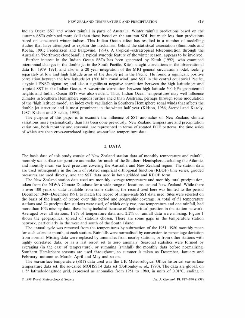
The New Zealand station data used are monthly average temperature and monthly total precipitation,taken from the NIWA Climate Database for a wide range of locations around New Zealand. While thereis over 100 years of data available from some stations, the record used here was limited to the periodDecember 1949–December 1991, to match the record of larger-scale SST data used. Sites were selected onthe basis of the length of record over this period and geographic coverage. A total of 51 temperaturestations and 74 precipitation stations were used, of which only two, one temperature and one rainfall, hadmore than 10% missing data, these being included because of their critical position in the station network.Averaged over all stations, 1.9% of temperature data and 2.2% of rainfall data were missing. Figure 1shows the geographical spread of stations chosen. There are some gaps in the temperature stationnetwork, particularly in the west and south of the South Island.

The annual cycle was removed from the temperatures by subtraction of the 1951–1980 monthly meanfor each calendar month, at each station. Rainfalls were normalised by conversion to percentage deviationfrom normal. Missing data were replaced by anomalies from nearby stations, or from other stations withhighly correlated data, or as a last resort set to zero anomaly. Seasonal statistics were formed byaveraging (in the case of temperature), or summing (rainfall) the monthly data before normalising.Southern Hemisphere seasons are used throughout, so summer is taken as December, January andFebruary; autumn as March, April and May and so on.

The sea-surface temperature (SST) data used was the UK Meteorological Office historical sea-surfacetemperature data set, the so-called MOHSST4 data set (Bottomley et al., 1990). The data are global, ona 5° latitude/longitude grid, expressed as anomalies from 1951 to 1980, in units of 0.01°C, ending in


A.B. MULLAN820

December 1991. There is a great deal of missing data prior to about 1950, and also south of about 50°S,which influenced the choice of study area and data period. For this study, data were used over the region12.5°N–57.5°S by 47.5°E–282.5°E, for the period December 1949–December 1991. This area encloses thetropical Pacific region known to be important from ENSO studies, and the tropical Indian Ocean regionidentified in Nicholls (1989) as having teleconnections to Australian rainfall. A subset of this area,covering 22.5°S–52.5°S by 147.5°E–197.5°E (77 grid points), was used to generate REOFs of ‘local’ SSTpatterns, in the study of air–sea interaction close to New Zealand (Section 4), whereas the full area wasused in the cross-correlation analysis of teleconnections (Section 5). Missing data was set to zero anomalyfor seasonal calculations.

The MSLP fields are taken from the regional gridded data set maintained by NIWA (Kidson andBarnes, 1984) for the period July 1957 through to December 1979, and from analyses issued by theEuropean Centre for Medium-range Weather Forecasts (ECMWF) for the period from January 1980.These MSLP data are on a latitude–longitude grid, extending from 5°S to 80°S in 5° steps and from 60°Eto 150°W in 10° steps. A sub-region, 20°S–60°S by 140°E–200°E, within which there was no missing dataover 1957–1991, was used. The annual cycle was removed by subtraction of the long-term mean pressurefor each month at each grid point. Note that this data set does not begin as early in time as the NewZealand climate and SST data.

3. ANALYSIS CONSIDERATIONS

3.1. Rotated empirical orthogonal functions

EOF analysis is a useful data description/compression technique, which aims to account for themaximal amount of variance in a data set with the minimal number of parameters. The technique wasapplied here, with subsequent varimax rotation, to New Zealand rainfall and temperature data, and alsoto gridded SST data in the local New Zealand region.

Figure 1. Geographical distribution of (a) the 51 temperature sites, and (b) the 74 rainfall sites used in this study



Empirical orthogonal function (EOF) analysis was applied separately to both monthly and seasonaldata, using all months (or seasons) together. This type of analysis produces spatial patterns of climateanomalies, with an associated time series of amplitude coefficients (or principal component scores). WhileEOFs are a useful way of compressing variance information in a data set, the physical interpretation ofthe EOF patterns is unclear, with the EOFs often not corresponding well with typical observed patternsof variability in the data. Unrotated EOFs usually form a predictable set of patterns, where the firstcomponent pattern has a high loading over much of the domain, and subsequent components are dipolesor more complex patterns. Richman (1986) recommends that rotating some of the components isadvantageous, and a varimax rotation was applied in this instance. This is one of the most widely usedrotation techniques, and has been shown to produce stable patterns (e.g. Cheng et al., 1995).

Rotation acts to isolate subgroups of stations that covary similarly, and thus is useful for regionalisingthe variations. The rotation generally produces a simpler set of patterns, often with a single stronganomaly of one sign in part of the domain, in contrast to the bipolar or more complex higher orderunrotated EOFs. Although various measures have been devised to estimate the statistical significance ofthe EOF components (Richman, 1986), there is no generally accepted criterion for deciding how manycomponents to rotate. Rotating too many components (overrotation) results in excessive regionalisationof the patterns, whereas rotating too few components (underrotation) can distort the patterns. We haveconsidered Kaiser’s criterion (Kaiser, 1958), where eigenvectors with eigenvalues greater than 1 (derivedfrom a correlation matrix) are retained for rotation; and also the scree test (Cattel, 1966; Craddock andFlood, 1969) where a break in the slope of plotted eigenvalues (or log of eigenvalue) is used to separateretained eigenvectors from the noise. Rotation was applied using differing numbers of eigenvectors nearthat number suggested by either the Kaiser or scree criteria, and emphasis given to readily interpretablestable patterns. Figures 2–4 show the REOF patterns with the rotations finally decided upon, and TableI lists the corresponding explained variances. The analysis was repeated for seasonal data, and virtuallyidentical REOFs obtained: the explained variances (bracketed values in Table I) were usually very similarto the monthly results.

For temperature, three eigenvectors are retained for rotation, and the REOF patterns illustrated inFigure 2. We can identify the regionalised responses as a North Island pattern (REOF 1), an east coastpattern (REOF 2) and a west coast South Island pattern (REOF 3). Note that REOF 3 has a dipolarpattern, of lower temperatures on the North Island east coast associated with higher west coast SouthIsland temperatures. Rotating more eigenvectors does not remove this dipolar characteristic, and insteadintroduces more complex patterns beyond REOF 3. We have high confidence in the stability of theseREOFs. Salinger and Mullan (1996) also calculated rotated temperature EOFs for New Zealand, usingsomewhat different data sets for the overlapping periods 1930–1975 and 1951–1994. Although theseREOFs explained quite different amounts of variance during the two time periods, the REOF patternsthemselves were very similar, and also closely matched those of Figure 2. The seasonal REOF patterns arealso shown in Figure 2 for comparison. The main difference occurs in REOF 3, where the seasonalpattern has a more prominent secondary maximum in the northwest of the South Island.

The 6 monthly rainfall REOFs are shown in Figure 3, where regionalisation occurs in the east SouthIsland (REOF 1) and east North Island (REOF 2), northern North Island (REOF 3), southwest SouthIsland (REOF 4) and North Island (REOF 6), and northeast South Island (REOF 5). These regionscorrespond well with typical weather forecast districts used by MetService New Zealand, and areexplainable in terms of the strong orographic control on New Zealand rainfall (Salinger, 1981). Seasonaldata produces rotated patterns that can be matched with those of Figure 3 although, as Table I shows,the explained variances are slightly different. In all cases, we order the REOFs by decreasing explainedvariance in the monthly patterns.

Figure 4 shows the 6 monthly SST patterns over the local New Zealand region, that regionalise overdifferent parts of the domain. The data resolution means that the contours cross New Zealand, althoughnot Australia. The first and most important REOF is centred more or less over New Zealand, whichjustifies a posteriori the use of a ‘New Zealand average’ SST anomaly by Basher and Thompson (1996).It was noted previously that there is considerable missing data in the southern part of the SST domain.


A.B. MULLAN822

Figure 2. The leading three rotated EOFs of New Zealand mean temperature anomalies, for monthly data (top row), and seasonaldata (bottom row), for all months or seasons of the year. Isopleths of the pattern weightings are plotted every 0.1, with negativeisopleths dashed and the zero isopleth dotted. The percentage variance accounted for by the REOF is shown within each panel

Attempts were made to interpolate and fill in missing values; this process still produced much the samepattern of REOFs, although the explained variance of the higher latitude patterns (REOFs 3 and 4) wascorrespondingly increased. Hence, we believe the SST REOFs are also stable. The patterns of Figure 3 canalso be related to those of Whetton (1990a), who calculated seven REOFs (that he labelled T1–T7) fromAustralian Bureau of Meteorology SST data for 1973–1980. For the region where our two domainsoverlap, our REOF 1 can be matched to Whetton’s T3, and also our REOFs 2, 5 and 6 to Whetton’s T7,T5 and T4, respectively.

It is also worth noting that all the seasonal SST REOFs have significant correlations (at 95%significance) with the SOI in at least one season of the year (not shown), with the strongest ENSOassociations (99% significance level) being with REOF 2 and REOF 5 in winter and spring. In these twoseasons, the same REOFs (2 and 5) also have significant interseasonal (monthly) correlation with the SOI.These REOFs are probably indicative of SST fluctuations south of the South Pacific convergence zone(REOF 2), and in the East Australia Current (REOF 5). The REOF 5 relationship is consistent with thefindings of Hirst and Godfrey (1993) that changing the amount of Indonesian oceanic throughflow to theIndian Ocean produces large variations in the East Australian Current and in surface temperatures in the



Tasman Sea. Opening and closing the Indonesian throughflow acts as a proxy for lower and higher sealevels, respectively, and other current changes in the tropical western Pacific that occur with ENSOvariations.

3.2. Cross-correlations and prewhitening

In Section 5 an exploratory analysis is carried out using SST data over the extended region12.5°N–57.5°S by 47.5°E–282.5°E, to look for possible predictors of the New Zealand climate dataREOF patterns. The approach used is a standard one of calculating lagged linear correlations, but a veryimportant consideration is how statistical significance of the resulting correlations is assessed. Onetechnique that is common in the meteorological literature is that of Davis (1976), also described byTrenberth (1984), whereby the number of degrees of freedom is reduced according to the degree of lagautocorrelation (persistence) in the data series used. An alternative technique of ‘prewhitening’, themethod adopted in this paper, is strongly recommended by Katz (1988) when searching for teleconnec-

Figure 3. The leading six rotated EOFs of New Zealand monthly mean rainfall anomalies, for all months of the year. Isopleths asFigure 2


A.B

.M

UL

LA

N824

©1998

Royal

Meteorological

SocietyInt.

J.C

limatol.

18:817

–840

(1998)

Figure 4. The leading six rotated EOFs of monthly mean SST anomalies over the New Zealand region, for all months of the year. Isopleths as in Figure 2. The percentagevariance accounted for by the REOF, and the REOF number, is given above each panel


Table I. Explained variance (%) of rotated EOFs for New Zealand temperature andrainfall, and regional SST, using either monthly or seasonal (bracketed values) data

REOF no. Temperature Rainfall SST

1 46.4 (47.1) 15.5 (16.0) 11.5 (15.4)2 29.3 (29.4) 13.3 (11.6) 8.1 (10.6)3 10.7 (9.6) 11.5 (12.3) 7.8 (10.2)4 11.5 (12.4) 7.1 (9.0)5 9.6 (10.0) 6.6 (8.0)6 8.4 (7.9) 6.5 (7.9)Total 86.2 (86.1) 69.8 (70.0) 47.6 (61.0)

tions in meteorological data. Prewhitening removes the autocorrelation in each time series involved, andit is the residual series (the so-called innovation series) that are cross-correlated. This results incorrelations generally smaller in magnitude than those produced from the original series but, since theinnovation series have near-zero persistence, the full number of data points is now used to estimatesignificance levels from a simple Student’s t-test. The areal coverage of significant regions of cross-corre-lation should be comparable in the two techniques, although the numerical value of the correlations willdiffer between the Trenberth (1984) and Katz (1988) approaches.

In this paper, prewhitening is done by calculating the innovation time series using the algorithm of Katz(1988). It should be mentioned that prewhitening is probably more common in fields such as hydrologyand fisheries than in atmospheric sciences. It is not normally used in deriving statistical predictionrelationships; its main value is in inferring cause and effect in lag relationships where persistence is presentin the basic data series. Katz (1988) showed that the effect of autocorrelation in the individual time seriesis to introduce non-zero cross-correlations at non-zero lags, even if there is no real interrelationshippresent. This would obviously be a problem with SST data where 1-month lag autocorrelations can be aslarge as +0.7, especially if cross-correlating SST against NZ land temperature data which also hasconsiderable persistence. A final point about the method that should be emphasised is that withprewhitened data the correlations on seasonally stratified monthly data effectively describe month tomonth relationships within a season. Research has shown that it is generally more difficult to predictvariations within a season than variations of the season as a whole (Rowell et al., 1995).

As an example of how prewhitening can clarify SST–climate relationships, we present Figures 5 and 6,that show correlations between the SST field and New Zealand temperature REOF 1 (North Island,Figure 2) for monthly data over the summer period (December, January, February). The effect ofprewhitening (Figure 5(a), 6(a)) or not (Figure 5(b), 6(b)) is contrasted, for both the contemporarycorrelation (Figure 5) and for 1-month lag (Figure 6) with sea temperature leading. Note that seasonallystratified lag results presented throughout this paper represent correlations ending during the specifiedseason (i.e. in the case of Figure 6 we have November–December, December–January and January–February). On the basis of the raw correlations (Figure 5(a), 6(a)) we would identify two main geographicregions where sea-surface temperature anomalies appear related to New Zealand North Island tempera-ture fluctuations: very strong positive correlations occur with SSTs around New Zealand and extendingnorth-northwest to Indonesia, and contrasting negative correlations with SST in the tropical east Pacific(the so-called NINO-3 region). Both these relationships appear physically reasonable. We know, forexample, that ENSO events affect New Zealand temperatures, such that colder conditions occur duringEl Nino (warm tropical SSTs) and 6ice 6ersa for La Nina (Gordon, 1986; Mullan, 1995). There appearsto be both a contemporary relationship (Figure 5(a)) and a weaker lag relationship (Figure 6(a)).

However, the prewhitened results necessitate a somewhat different interpretation. While the contempo-rary correlation (Figure 5(b)) is only slightly weaker around New Zealand, the signal has disappearedalmost entirely in the tropical Pacific. Thus the innovation series of NZ temperature and local SST stillvary together, but there is no ENSO signal at the intermonthly timescale. The apparent ENSO signal fromFigure 5(a) is therefore due to persistence in the sea temperature field. Furthermore, when 1-month lag is


A.B. MULLAN826

considered (Figure 6(b)), temperature REOF 1 no longer has any relationship to local SST variationseither. Land temperature anomalies in one month are related only to SST anomalies in the same month,but high persistence in both series means land temperature anomalies are often similar to the previousmonth’s SST departures. It would be wrong however to conclude naively (from Figure 6(a)) that any reallag association exists. The conclusion then is that, when persistence effects have been discounted, NewZealand land temperatures and nearby sea temperatures do indeed vary together concurrently (exploredfurther in the following section), but that there is no lag relationship with SST leading, at least forsummer. At this intermonthly timescale, although not interseasonal (see later), there appears to be noENSO signal either.

All cross-correlations presented subsequently in this paper are between prewhitened time series.Significance is assessed at the 2-sided 95% level using the Student’s t-test.

4. LOCAL SST–CIRCULATION INTERACTIONS

As many authors have noted, it is difficult to unravel the relationships between SST and air circulationanomalies because of the strong coupling between the oceanic and atmospheric media (e.g. Namias andCayan, 1981). Many physical arguments can be advanced for possible interactions, and patterns ofresponse of one media to the other appear not to be unique. However, a close examination of Figure 7suggests the most important physical processes operating at the New Zealand regional scale. In this figure

Figure 5. Contemporary correlation (×100) between SST over domain shown and New Zealand temperature REOF 1, withoutprewhitening (a) and with prewhitening (b) of both series. Shading indicates significance at 95% level based on number of months

in sample (42 years by 3 months)



Figure 6. As Figure 5, but for 1-month lag correlations where sea temperature leads REOF 1

the contemporary and lead/lag correlations between the SST REOF patterns of Figure 4 and MSLPanomalies are displayed. All data are monthly and there is no seasonal stratification. Shading denotescorrelations significant at the 95% level, and the correlation patterns can be interpreted like a pressureanomaly map. The strongest interactions are clearly the contemporary ones (top row of panels in Figure7), followed by those where MSLP leads by 1 month (middle row), with the SST-lead correlations (bottomrow) the weakest of all.

If the contemporary SST–MSLP correlations are compared with the SST REOF patterns themselves(Figure 4), we see a very clear relation between the location of the regionalised SST peak response andthe location of strongest northerly (or northwesterly/northeasterly) gradient flow in the pressure anoma-lies. For example, high positive (negative) values of REOF 1 are associated with strong northeast(southwest) airflow anomalies, and this behaviour is consistent across all six SST REOF patterns. Thispattern of positive MSLP anomalies to the east of the SST maximum can be readily explained in termsof the atmospheric circulation forcing the oceanic anomalies through a combination of advection and heatfluxes. More northerly sector airflow advects warmer surface water and air southward. Heat fluxes fromocean to atmosphere are reduced because of the warmer overlying air and generally lighter winds (themean flow is westerly all year round south of about 37°S), resulting in higher sea-surface temperatures.It is beyond the scope of the present study to go one step further and determine which of these physicalprocesses dominate.

Given these strong contemporary relationships between monthly SST and atmospheric circulation, it isno surprise that the SST REOF patterns also show significant correlations with the New Zealandtemperature and rainfall patterns of Figures 2 and 3. For example, SST REOF 1 has a very significantpositive correlation with all the temperature REOFs: conditions are warmer everywhere during months


A.B

.M

UL

LA

N828

©1998

Royal

Meteorological

SocietyInt.

J.C

limatol.

18:817

–840

(1998)

Figure 7. Correlations (×100) of monthly mean MSLP anomalies with New Zealand region SST REOFs 1–6. Results are shown for simultaneous correlations (top row), whereMSLP leads by 1 month (centre row), and where SST leads (bottom row). Shading denotes correlations significant at 95% level


with northerly flow anomalies. SST REOF 6 is negatively correlated with concurrent New Zealandrainfall, particularly rainfall REOFs 3, 5 and 6. However, it would not be reasonable to argue that themonthly climate anomalies are caused by the SST anomalies; both are clearly related to atmosphericcirculation fluctuations.

The patterns of Figure 7 were calculated using all months together; that is, no seasonal stratification isconsidered. We will not present such results here, but it is worth noting that there is certainly a seasonaldependence in the significance of the correlations, In general, simultaneous correlations between circula-tion and SST anomalies are markedly weaker in the winter season. It is likely that sea-surfacetemperatures are more sensitive to atmospheric variations in the summer half-year when oceanicthermocline depths are shallower and vertical mixing is reduced.

The central row of Figure 7 where MSLP leads by 1 month suggests a different process is effectingoceanic changes over a slightly longer timescale. With the exception of REOF 5, these correlations showthat higher (lower) MSLP in 1 month is co-located with higher (lower) SST in the month following. Thissuggests that either radiative or downwelling effects are operating to alter sea temperatures at 1-monthlag. Under an anticyclonic anomaly, skies will be clearer and more radiation will reach the sea-surface;furthermore, convergence of surface waters will occur in the centre of the high pressure anomaly, alsoleading to higher surface temperatures. Why does REOF 5 not behave in quite the same way? It is likelythat changes in this REOF pattern reflect fluctuations in the East Australian Current, which is asouthward flowing ocean current off the eastern coast of Australia, and a major oceanographic feature ofthe region (Heath, 1985). The East Australian Current is known to be influenced at least partially byfactors remote from the region of Figure 7 (Hirst and Godfrey, 1993).

The cross-correlations with SST leading by 1 month (bottom panels of Figure 7) are very weak whenall months are combined, but there is some suggestion that higher (lower) sea-surface temperatures in 1month result in lower (higher) MSLP anomalies somewhat equatorward in the following month.Anomalous warm water favours enhanced cyclonic activity (and therefore lower MSLP) throughincreased sensible and latent heating and vertical destabilisation of the atmosphere, and 6ice 6ersa forcolder water. Ratcliffe and Murray (1970) found such 1-month lag relationships in the North Atlanticbetween SST and subsequent MSLP anomalies. The MSLP anomaly o6er the SST anomaly was ratherweak, but stronger MSLP anomalies of alternating sign occurred downstream in a wavetrain pattern.Unfortunately, our MSLP data does not extend far enough east of New Zealand to enable any possibledownstream influence to be identified.

Thus, Figure 7 leads to the conclusion that there is a strong simultaneous relationship between SST andMSLP patterns with the atmosphere forcing the ocean, a moderate 1-month lag association with MSLPleading, and a very weak (at least locally) 1-month lag relationship with SST leading.

5. HEMISPHERIC SST INFLUENCE ON NZ CLIMATE

In this section, we make a systematic exploration for SST–climate relationships over a much widergeographic region than in Section 4, and also stratify the results to accommodate seasonally varyingrelationships, as have been found by other studies. Both 1-month lags (stratified by season) andone-season lags between SST gridpoint data and each rainfall and temperature rotated EOF wereexamined. In many cases, the pattern of monthly lag correlations is similar to that of the seasonal lags,although it is usually weaker and often not statistically significant. Many of the lag relationships appearto be ENSO related, although not necessarily just with tropical Pacific SSTs. We highlight below onlythose correlations which are strongest, cover a number of grid-points, and are amenable to some physicaljustification. As noted previously, the SST data are sparse south of 50°S, and occasional large correlationsfound at these latitudes are ignored. While significance of the correlations is calculated at each grid-point,for purposes of presentation we have subsequently smoothed the correlation coefficients and associatedt-values with a simple two-dimensional binomial filter before plotting the results: this tends to eliminateisolated high correlations.


A.B. MULLAN830

Since ENSO-related SST patterns will figure prominently in the following results, it is helpful to beginwith Figure 8, showing the simultaneous correlation between Southern Oscillation Index (SOI) and SST.The calculation is done for seasonal data, all seasons together. In the Pacific, there is a broad band ofnegative correlations along the equator from about 180° eastwards, together with a band of positivecorrelation to the south that extends from Indonesia east-southeastwards into the central South Pacific.The diagonal line where the correlation reverses sign approximates the location of the South Pacificconvergence zone. Seasonally, this pattern is strongest in winter and spring, with the spring patternemphasising the subtropical SSTs such that the region of significant correlations extends around northernNew Zealand (i.e. sea temperatures around New Zealand are colder during El Nino). Similar, but weaker,Pacific SST patterns occur in summer and autumn. Seasonally, there is also a significant SOI correlationwith Indian Ocean SSTs near 15°S, 90°E that is negative in summer and winter and positive in spring. Thenegative SST–SOI correlation in the Pacific north and east of New Zealand (Figure 8) agrees with stationair temperature relationships described by Halpert and Ropelewski (1992).

Looking now at lag relationships between SST and New Zealand climate REOFs, Figure 9 shows twoexamples of 1-month lag calculations. Both Figure 9(a) and (b) are for temperature, which generally havebetter relationships with SST than does New Zealand rainfall at the 1-month timescale. Figure 9(a) showsthat temperature REOF 1 (North Island, see Figure 2) during autumn months (March, April, May) ispositively correlated with the previous month’s SST anomalies in the western Tasman Sea and theAustralian Bight. The fact that the SST region indicated is just upstream of New Zealand in the prevailingatmospheric and oceanic flow suggests that advection may play a role here (see later discussion). A similarSST pattern occurs with South Island temperatures (REOFs 2 and 3, not shown), although the SSTrelationship with REOF 1 is strongest. There does not appear to be any influence on New Zealand rainfallin autumn at 1-month lag. This positive association between New Zealand temperatures and upstreamSST also does not occur at other times of year outside the autumn season.

Figure 9(b) shows a quite different 1-month lag correlation pattern between August, September andOctober SSTs and temperature REOF 2 during spring months. Similar but weaker correlation patternsoccur with temperature REOFs 1 and 3, and also for rainfall REOF 1 but with reversed sign to thecorrelations. Thus, higher temperatures and lower rainfalls on the east coast of the South Island in springare associated with the SST pattern of Figure 9(b). The correlations show higher SSTs south of the SouthPacific convergence zone and lower SSTs to the north, along with higher SSTs in the eastern Indian Oceanand around Indonesia, correspond to warmer temperatures over New Zealand. This pattern is reminiscentof the ENSO signal in sea-surface temperatures (Figure 8), which is most prominent during the springseason. There is also evidence of an enhanced wave 3 pattern (note SST anomaly dipoles at 90°E and150°W), or alternatively a change in zonality (SST anomalies at 20–30°S have generally opposite sign to

Figure 8. Contemporary seasonal correlation (×100) between SOI and SST, all seasons combined. Shading denotes correlationssignificant at 95% level



Figure 9. Lagged cross-correlations, using prewhitened monthly data, between sea-surface temperature and New Zealand climateREOFs: 1-month lag to (a) temperature REOF 1 ending autumn months, and (b) temperature REOF 2 ending spring months.

Shaded regions have correlations significant at 95% level or above

those south of 40°S). Higher temperatures and lower rainfall on the east of the South Island are also whatone would expect with stronger zonal flow across New Zealand. Further analysis is required to determinewhether this variation in SST zonality is related in any way to the high latitude mode fluctuations ofKidson (1986).

There is little in the way of coherent SST monthly lag correlation patterns with New Zealand climatein summer. In winter, all three temperature REOFS and rainfall REOFs 3, 5 and 6 have a significantnegative correlation with the previous month’s SST anomaly near the equator at 120°W–90°W in theeastern tropical Pacific. This would appear to be a weak intermonthly ENSO signal, consistent with coldertemperatures and drier conditions that prevail in the east and north of both islands during El Ninos or‘warm events’ (Gordon, 1986).

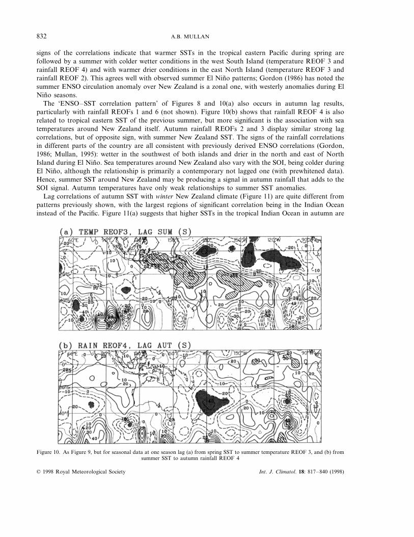
Seasonal lag correlations are generally stronger than monthly ones, and indicate useful SST relation-ships with New Zealand rainfall as well as temperature. The correlation patterns outside of the winterseason suggest mainly ENSO influences. Figure 10 shows two examples from the summer and autumnseasons. In Figure 10(a), spring SST is correlated against summer temperature REOF 3, and in Figure10(b), summer SST against the following autumn rainfall REOF 4. Figure 10(a) shows the SSTcorrelation pattern in the Pacific that recurs frequently with other REOFs and seasons, and that isassociated with the El Nino–Southern Oscillation (Figure 8).

The marked summer lag correlations (Figure 10(a)) for temperature REOF 3 do not occur for the othertemperature REOFs (see Figure 2). However, the rainfall REOFs 2 and 4 (see Figure 3) do display asimilar (except for sign) lag correlation pattern with Pacific sea temperatures of the previous spring. The


A.B. MULLAN832

signs of the correlations indicate that warmer SSTs in the tropical eastern Pacific during spring arefollowed by a summer with colder wetter conditions in the west South Island (temperature REOF 3 andrainfall REOF 4) and with warmer drier conditions in the east North Island (temperature REOF 3 andrainfall REOF 2). This agrees well with observed summer El Nino patterns; Gordon (1986) has noted thesummer ENSO circulation anomaly over New Zealand is a zonal one, with westerly anomalies during ElNino seasons.

The ‘ENSO–SST correlation pattern’ of Figures 8 and 10(a) also occurs in autumn lag results,particularly with rainfall REOFs 1 and 6 (not shown). Figure 10(b) shows that rainfall REOF 4 is alsorelated to tropical eastern SST of the previous summer, but more significant is the association with seatemperatures around New Zealand itself. Autumn rainfall REOFs 2 and 3 display similar strong lagcorrelations, but of opposite sign, with summer New Zealand SST. The signs of the rainfall correlationsin different parts of the country are all consistent with previously derived ENSO correlations (Gordon,1986; Mullan, 1995): wetter in the southwest of both islands and drier in the north and east of NorthIsland during El Nino. Sea temperatures around New Zealand also vary with the SOI, being colder duringEl Nino, although the relationship is primarily a contemporary not lagged one (with prewhitened data).Hence, summer SST around New Zealand may be producing a signal in autumn rainfall that adds to theSOI signal. Autumn temperatures have only weak relationships to summer SST anomalies.

Lag correlations of autumn SST with winter New Zealand climate (Figure 11) are quite different frompatterns previously shown, with the largest regions of significant correlation being in the Indian Oceaninstead of the Pacific. Figure 11(a) suggests that higher SSTs in the tropical Indian Ocean in autumn are

Figure 10. As Figure 9, but for seasonal data at one season lag (a) from spring SST to summer temperature REOF 3, and (b) fromsummer SST to autumn rainfall REOF 4



Figure 11. As Figure 9, but for autumn SST to winter climate patterns (a) for temperature REOF 3, and (b) for rainfall REOF 2

associated with higher west South Island temperatures in the following winter. A similar correlationoccurs with temperature REOF 2, and a similar but much weaker one with REOF 1, indicating thetemperature influence affects mainly the South Island. Indian Ocean SSTs between 60°E and 90°E, and0–20°S, also have significant positive correlations with winter rainfall REOF 4 and negative correlationswith REOFs 1, 2 (Figure 11(b)), 3, and 5. This pattern has similarities to the teleconnection identified byNicholls (1989) which affected Australian winter rainfall, and has subsequently been related to northwestclouds bands that affect Australia in that season.

Lag correlations of winter SST with spring climate anomalies show a mixture of the patterns previouslydescribed. The strongest lag relationships occur for temperature REOF 1 (Figure 12(a)), and for rainfallREOFs 2 (Figure 12(b)) and 3 (not shown). Again, this is in agreement with ENSO studies (Gordon,1986; Mullan, 1995) that show the strongest ENSO signal over New Zealand for spring is in the NorthIsland. In addition to the Pacific ENSO pattern in the correlation field, spring climate conditions overNorth Island have a significant relationship with winter SST around and to the north of New Zealand.Warmer waters there in winter result in warmer drier North Island conditions in spring, and 6ice 6ersa.In the case of the two rainfall REOFS (2 and 3), there is also a significant positive correlation with winterSST in the Indian Ocean to the west of Australia—this region being to the southeast of the region foundimportant for winter New Zealand climate. To what extent these Indian Ocean and New Zealand regionSSTs vary independently of the SOI needs to be investigated further.


A.B. MULLAN834

6. DISCUSSION

The approach taken in this paper of summarising New Zealand climate patterns by rotated EOFs, andthen cross-correlating the EOF time series against sea-surface temperature and mean sea level pressure,has proved a very fruitful one. Clear and consistent evidence has been presented that at the 1-monthtimescale, SST anomalies in the New Zealand region are forced by atmospheric fluctuations, bothsimultaneously and with MSLP leading by 1 month. Only very weak associations occur with local SSTleading atmospheric circulation in the region by 1 month, when all months of data are consideredtogether. Prewhitening of all data, as recommended by Katz (1988) was essential to interpreting theresults. When the SST–climate correlations are stratified seasonally, significant lag associations are foundwith sea temperatures over a wide region of the Southern Hemisphere.

Figure 13 summarises the results of the previous section in terms of ‘key areas’ where SST anomaliesappear to bear the greatest relationship to New Zealand climate fluctuations. Time series ‘indices’ weregenerated by averaging the SST anomalies over the regions indicated, and in Table II the seasonalsimultaneous correlation of each key area index with the SOI is given. SST1 measures SST anomalies localto New Zealand. Its value as a predictor is that it has a significant one season lead correlation with theautumn rainfall anomalies of REOF 2, 3, and 4, and with the spring rainfall anomalies of REOF 2 and3. SST1 is also included because of strong persistence in SST throughout the year, particularly in summer.Although the prewhitening technique specifically removes persistence, we recognise that persistence is animportant predictor, and the ultimate purpose of exploratory studies such as this would be long-rangeprediction of climate variability. SST2 delineates the region that leads autumn temperatures by 1 month,

Figure 12. As Figure 9, but for winter SST to spring climate patterns (a) for temperature REOF 1, and (b) for rainfall REOF 2



Figure 13. SST index ‘key areas’, delineating regions that have significant lag correlations with New Zealand temperature andrainfall

and also matches well the T4 SST REOF pattern of Whetton (1990a). Indices SST3 and SST4 are theso-called NINO3 and NINO4 regions, respectively, that are frequently used to monitor the status of theEl Nino–Southern Oscillation. Indices SST5 and SST6 to the north and eastnortheast of New Zealandappear to be particularly important for spring and summer climate at one season lead, and are stronglyrelated to the SOI also. In addition, SST6 is the only region other than SST2 that has significantcorrelation to New Zealand climate at 1-month lag (Figure 9(b)). The Indian Ocean influences arerepresented by SST7, SST8 and SST9, none of which show much relation to the SOI outside summer. Theapparently slight displacement in regions affecting winter temperature (SST7) and rainfall (SST8) may bean artifact of the limited data set we are using. The Australian rainfall predictor used by Nicholls (1989)was defined as the SST gradient between Indonesia (0–10°S, 120–130°E) and the central Indian Ocean(10–20°S, 80–90°E), and is negatively correlated with the indices SST7–SST9.

Most of the SST–New Zealand climate relationships found occur at the seasonal timescale, with ENSOteleconnections figuring prominently, in agreement with previous investigations into SOI correlations(Gordon, 1986; Mullan, 1995). However, two particular new results will be discussed further here: the1-month lag association between key area 2 SSTs and autumn temperatures, and the seasonal lagassociation between the key areas indices in the Indian Ocean and winter rainfall and temperatures.

Figure 9(a) suggests that higher sea temperatures in the Australian Bight and western Tasman inFebruary, March or April result in higher North Island temperatures the following month. Note thatFigure 9(a) shows no lag correlation with SSTs immediately adjacent to New Zealand, as would appearto be the case if the data series were not first prewhitened. The immediately upstream location of the SSTanomaly pattern with respect to New Zealand means that direct advective effects must be considered. Airflow over warmer seas south and west of Australia might subsequently result in relatively warmer airreaching New Zealand, although why there should be a 1-month lag, and the relationship hold only inautumn, is unclear. Advection of SST anomalies by ocean currents is also a possibility. The surface

Table II. Simultaneous prewhitened correlations between SOI and the key area SST indicesfor the regions of Figure 13, using seasonal data over the period 1949–1991. Results are

shown only for correlations significant at 95% or above

SST1 SST2 SST3 SST4 SST5 SST6 SST7 SST8Season SST9

−0.35 −0.30Summer −0.38−0.38−0.43*Autumn

Winter −0.48* −0.62* 0.43* 0.46*0.43* 0.57*0.67*−0.58*Spring −0.31

* Indicates significance at 99%.


A.B. MULLAN836

Figure 14. As Figure 9(a), but correlations calculated separately for first and second halves of the data set. (a) First half, 1950–1970;(b) second half, 1971–1991

current flow in the Tasman Sea is generally eastward towards New Zealand (Heath, 1985), with the flowbeing diverted around New Zealand either to the north (by the ‘Tasman Current’) or the south. TheTasman Current is particularly prominent, and would be consistent with North Island temperatures(REOF 1) being most responsive to SST anomalies off southeastern Australia. Measurements of currents,and particularly their seasonal variability, are scarce (Hamilton, 1992), but what measurements existsuggest that current speeds are too low to advect SST anomalies close to New Zealand within the monthlytimeframe. The UK Meteorological Office (1967) quarterly charts suggest current speeds on the order of20 km day−1 (0.23 ms−1), implying about 3 months to cross the Tasman.

In any exploratory study, there is always the possibility that significant correlations have still occurredby chance, as a result of the particular data set used. Figure 14(a, b) shows the 1-month lag correlationof Figure 9(a) repeated for the first and second halves of the 42-year data set. The SST correlation withautumn temperature REOF 1 (and REOFs 2 and 3) appears to be stable since it occurs in bothsubperiods, although the main correlation lobe is closer to New Zealand in the 1950–1970 period, andstronger and further west in 1971–1991. Figure 15 reinforces that idea that SST anomalies south andsoutheast of Australia are somehow linked to New Zealand air temperatures through sea temperatureslocal to New Zealand. Figure 15 is a 1-month lag correlation with SST anomalies, similar to Figure 9(a),except that the lagged variable is not a temperature REOF but SST1, the sea temperature anomalyaround New Zealand (Figure 13). We see a pattern that is very similar to Figure 9(a), with SST anomaliessouth of Australia leading anomalies of the same sign around New Zealand by one month. Thisrelationship between SST1 and SST2 does not occur at other lags, such as 1 or 2 months or seasonal, orat other times of year outside autumn.



Figure 15. As Figure 9(a), but for 1-month lag from SST to autumn key area index SST1 (New Zealand)

The SST2 time series was also cross-correlated against MSLP data, as shown in Figure 16. At 1-monthlag (SST2 leading autumn MSLP, Figure 16(a)), there is no circulation anomaly associated with the SSTanomaly south of Australia and in the western Tasman. This is consistent with the finding previouslynoted that none of the New Zealand rainfall REOFs were associated with SST2, only the temperaturepatterns. There is a strong concurrent relationship between SST2 and atmospheric circulation (Figure16(b)), as expected from the discussion of local SST-circulation interactions of Section 4. We note too thatkey area SST2 approximates SST REOF 6 of Figure 4, and there is a similarity between the MSLPpattern of Figure 16(b) and the SST REOF 6 simultaneous correlation in Figure 7. Given these variousresults, it is our conclusion that the most likely cause of SST–New Zealand temperature lag correlationsin autumn is atmospheric forcing from the month previous. Northeasterly airflow anomalies between NewZealand and Tasmania in 1 month (Figure 16(b) and concurrent pattern of REOF 6 (in Figure 7) generatewarmer SSTs in key region 2. At the same time, the anticyclonic conditions extending over New Zealandalso lead, through the mechanisms discussed in Section 4, to warmer SSTs around New Zealand in the

Figure 16. Prewhitened cross-correlations (×100), using monthly data, between key SST index 2 (Australian Bight) and autumnMSLP in the New Zealand region. (a) SST2 leading MSLP by 1 month; (b) SST2 and MSLP concurrent. Shaded regions have

correlations significant at 95% level or above


A.B. MULLAN838

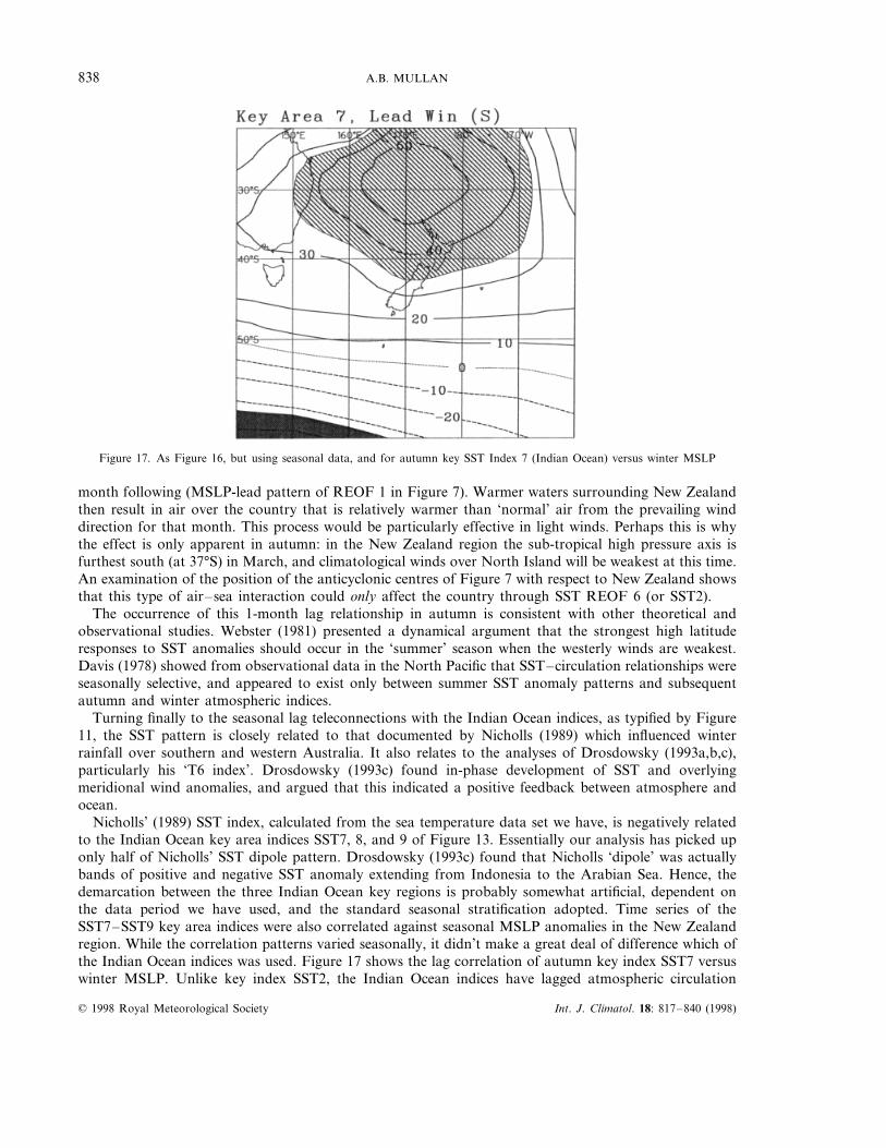
Figure 17. As Figure 16, but using seasonal data, and for autumn key SST Index 7 (Indian Ocean) versus winter MSLP

month following (MSLP-lead pattern of REOF 1 in Figure 7). Warmer waters surrounding New Zealandthen result in air over the country that is relatively warmer than ‘normal’ air from the prevailing winddirection for that month. This process would be particularly effective in light winds. Perhaps this is whythe effect is only apparent in autumn: in the New Zealand region the sub-tropical high pressure axis isfurthest south (at 37°S) in March, and climatological winds over North Island will be weakest at this time.An examination of the position of the anticyclonic centres of Figure 7 with respect to New Zealand showsthat this type of air–sea interaction could only affect the country through SST REOF 6 (or SST2).

The occurrence of this 1-month lag relationship in autumn is consistent with other theoretical andobservational studies. Webster (1981) presented a dynamical argument that the strongest high latituderesponses to SST anomalies should occur in the ‘summer’ season when the westerly winds are weakest.Davis (1978) showed from observational data in the North Pacific that SST–circulation relationships wereseasonally selective, and appeared to exist only between summer SST anomaly patterns and subsequentautumn and winter atmospheric indices.

Turning finally to the seasonal lag teleconnections with the Indian Ocean indices, as typified by Figure11, the SST pattern is closely related to that documented by Nicholls (1989) which influenced winterrainfall over southern and western Australia. It also relates to the analyses of Drosdowsky (1993a,b,c),particularly his ‘T6 index’. Drosdowsky (1993c) found in-phase development of SST and overlyingmeridional wind anomalies, and argued that this indicated a positive feedback between atmosphere andocean.

Nicholls’ (1989) SST index, calculated from the sea temperature data set we have, is negatively relatedto the Indian Ocean key area indices SST7, 8, and 9 of Figure 13. Essentially our analysis has picked uponly half of Nicholls’ SST dipole pattern. Drosdowsky (1993c) found that Nicholls ‘dipole’ was actuallybands of positive and negative SST anomaly extending from Indonesia to the Arabian Sea. Hence, thedemarcation between the three Indian Ocean key regions is probably somewhat artificial, dependent onthe data period we have used, and the standard seasonal stratification adopted. Time series of theSST7–SST9 key area indices were also correlated against seasonal MSLP anomalies in the New Zealandregion. While the correlation patterns varied seasonally, it didn’t make a great deal of difference which ofthe Indian Ocean indices was used. Figure 17 shows the lag correlation of autumn key index SST7 versuswinter MSLP. Unlike key index SST2, the Indian Ocean indices have lagged atmospheric circulation



anomalies associated with them. The subtropical ridge just north of North Island in winter is strongerwhen the sea-surface is warmer in the tropical Indian Ocean during the previous (or concurrent) season,and 6ice 6ersa. This atmospheric anomaly pattern in the Tasman is the same as that identified byDrosdowsky (1993c) for his T6 teleconnection pattern. Thus, for New Zealand the teleconnection patternis one of higher (lower) autumn SST in the central tropical Indian Ocean followed by winter New Zealandclimate anomalies of stronger (weaker) westerly flow over the country, with higher (lower) South Islandtemperatures, wetter (drier) in west South Island districts and drier (wetter) in all other areas exposed tothe north and east. The warmer South Island winters correspond to drier winters over southern Australia(Drosdowsky, 1993a,c).

The stability of this teleconnection was tested by calculating lag correlations with respect to the twohalves of the SST data set, as was done for SST2 (Figure 14). The result (not shown) was similar patternsfor the both 1950–1970 and 1971–1991 periods, although somewhat stronger in the earlier record. Wenote, however, that Drosdowsky (1993c) found the Indian Ocean teleconnection was not apparentlyoperating in pre-1950 data. Our analysis has also indicated a weaker winter Indian Ocean SST–springclimate teleconnection (involving region SST9, Figure 12). Here, such significant correlations as occur areof opposite sign to the autumn–winter ones. Thus, warmer (colder) subtropical waters in winter to thewest of Australia are associated with an anomalous spring trough (ridge) over North Island with wetter(drier) conditions in the east (rainfall REOF 2).

This study reinforces the importance of seasonal stratification when making long-range predictions.Different teleconnections and air–sea interactions appear to be operating at different times of year,necessitating the use of new predictors. In particular, the occurrence of significant Indian Ocean SSTpatterns, at the time of year when ENSO teleconnections are weaker, are encouraging for seasonalprediction of New Zealand climate anomalies. Future work should aim to quantify the skill of predictionsbased on Indian Ocean anomalies, perhaps using a technique such as rotated singular value decomposi-tion (Cheng and Dunkerton, 1995), and concentrating on the seasonal timescale rather than the monthlyone. Variations in key area SST2, and the concurrent atmospheric circulation, may also prove useful forpredicting intermonthly temperature variations during autumn.

ACKNOWLEDGEMENTS

The author is grateful to the UK Meteorological Office for making available the sea-surface temperature(MOHSST4) data set. This research was supported by the New Zealand Foundation for Research, Scienceand Technology under contract C01522.

REFERENCES

Basher, R.E. and Thompson, C.S. 1996. ‘Relationship of air temperatures in New Zealand to regional anomalies in sea-surfacetemperature and atmospheric circulation’, Int. J. Climatol., 16, 405–425.

Bottomley, M., Folland, C.K., Hsiung, J., Newell, R.E. and Parker, D.E. 1990. ‘Global ocean surface temperature atlas (GOSTA)’,Joint UK Meteorological Office/Massachusetts Institute of Technology Project, HMSO, London, 20+ iv pp and 313 plates.

Cattel, R.B. 1966. ‘The scree test for the number of factors’, Multi6ar. Beha6. Res., 1, 245.Cheng, X. and Dunkerton, T.J. 1995. ‘Orthogonal rotation of spatial patterns derived from singular value decomposition analysis’,

J. Climate, 8, 2631–2643.Cheng, X., Nitsche, G. and Wallace, J.M. 1995. ‘Robustness of low-frequency circulation patterns derived from EOF and rotated

EOF analyses’, J. Climate, 8, 1709–1713.Craddock, J.M. and Flood, C.R. 1969. ‘Eigenvectors for representing the 500 mb geopotential surface over the Northern

Hemisphere’, Q. J. R. Meteorol. Soc., 95, 576–593.Davis, R.E. 1976. ‘Predictability of sea-surface temperature and sea level pressure anomalies over the North Pacific Ocean’, J. Phys.

Oceanogr., 6, 249–266.Davis, R.E. 1978. ‘Predictability of sea level pressure anomalies over the North Pacific Ocean’, J. Phys. Oceanogr., 8, 233–246.Drosdowsky, W. 1993a. ‘Potential predictability of winter rainfall over southern and eastern Australia using Indian Ocean

sea-surface temperature anomalies’, Aust. Meteorol. Mag., 42, 1–6.Drosdowsky, W. 1993b. ‘An analysis of Australian seasonal rainfall anomalies: 1950–1987. I: Spatial patterns’, Int. J. Climatol., 13,

1–30.Drosdowsky, W. 1993c. ‘An analysis of Australian seasonal rainfall anomalies: 1950–1987. II: Temporal variability and teleconnec-

tion patterns’, Int. J. Climatol., 13, 111–149.


A.B. MULLAN840

Frankignoul, C. 1985. ‘Sea-surface temperature anomalies, planetary waves, and airsea feedback in the middle latitudes’, Re6.Geophys., 23, 357–390.

Frederiksen, C.S. and Balgovind, R.C. 1994. ‘The influence of the Indian Ocean/Indonesian SST gradient on the Australian winterrainfall and circulation in an atmospheric GCM’, Q. J. R. Meteorol. Soc., 120, 923–952.

Folland, C.K. and Salinger, M.J. 1995. ‘Surface temperature trends and variations in New Zealand and the surrounding ocean,1871–1993’, Int. J. Climatol., 15, 1195–1218.

Gordon, N.D. 1985. ‘The Southern Oscillation: a New Zealand perspective’, J. R. Soc. N. Z., 15, 137–155.Gordon, N.D. 1986. ‘The Southern Oscillation and New Zealand weather’, Mon. Wea. Re6., 114, 371–387.Graham, N.E., Barnett, T.P., Wilde, R., Ponater, M. and Schubert, S. 1994. ‘On the roles of tropical and midlatitude SSTs in

forcing interannual to interdecadal variability in the winter Northern Hemisphere circulation’, J. Climate, 7, 1416–1441.Halpert, M.S. and Ropelewski, C.F. 1992. ‘Surface temperature patterns associated with the Southern Oscillation’, J. Climate, 5,

577–593.Hamilton, L.J. 1992. ‘Surface circulation in the Tasman and Coral Seas: Climatological features derived from bathy-thermograph

data’, Aust. J. Mar. Freshw. Res., 43, 793–822.Haney, R.L. 1979. ‘Numerical models of ocean circulation and climate interaction’, Re6. Geophys. Space Phys., 17, 1494–1507.Heath, R.A. 1985. ‘A review of the physical oceanography of the seas around New Zealand—1982’, N. Z. J. Mar. Freshw. Res.,

19, 79–124.Hirst, A.C. and Godfrey, J.S. 1993. ‘The role of Indonesian throughflow in a global ocean GCM’, J. Phys. Oceanogr., 23,

1057–1086.Kaiser, H.F. 1958. ‘The varimax criterion for analytic rotation in factor analysis’, Psychometrika, 23, 187–200.Katz, R.W. 1988. ‘Use of cross correlations in the search for teleconnections’, J. Climatol., 8, 241–253.Kidson, J.W. 1986. ‘Index cycles in the Southern Hemisphere during the Global Weather Experiment’, Mon. Wea. Re6., 114,

1654–1663.Kidson, J.W. and Barnes, B.G. 1984. ‘Indices of the atmospheric circulation in the Australasian region’, N. Z. J. Sci., 27, 355–364.Kidson, J.W. and Sinclair, M.R. 1995. ‘The influence of persistent anomalies on Southern Hemisphere storm tracks’, J. Climate, 8,

1938–1950.Kitoh, A. 1992. ‘Tropical influence on the South Pacific double-jet variability’, in Preprint volume, Fourth International Conference

on Southern Hemisphere Meteorology and Oceanography, 29 March–2 April 1993, Hobart, pp. 48–49.Lanzante, J.R. 1984. ‘A rotated eigenanalysis of the correlation between 700 mb heights and sea-surface temperatures in the Pacific

and Atlantic’, Mon. Wea. Re6., 112, 2270–2280.Luksch, U. and von Storch, H. 1992. ‘Modeling the low-frequency sea-surface temperature variability in the North Pacific’, J.

Climate, 5, 893–906.Mullan, A.B. 1995. ‘On the linearity and stability of Southern Oscillation–climate relationships for New Zealand’, Int. J. Climatol.,

15, 1365–1386.Mullan, A.B. 1996. ‘Nonlinear effects of the Southern Oscillation in the New Zealand region’, Aust. Meteorol. Mag., 45, 83–99.Namias, J. and Cayan, D.R. 1981. ‘Large-scale air–sea interactions and short-period climatic fluctuations’, Science, 214, 869–876.New Zealand Official Yearbook 1994. Statistics New Zealand, Auckland, New Zealand, 567 pp.Nicholls, N. 1989. ‘Sea-surface temperatures and Australian winter rainfall’, J. Climate, 2, 965–973.Ratcliffe, R.A.S. and Murray, R. 1970. ‘New lag associations between North Atlantic sea temperature and European pressure

applied to long-range weather forecasting’, Q. J. R. Meteorol. Soc., 96, 226–246.Richman, M.B. 1986. ‘Rotation of principal components’, J. Climatol., 6, 293–335.Rowell, D.P., Folland, C.K., Maskell, K. and Ward, N. 1995. ‘Variability of summer rainfall over tropical north Africa (1906–92):

Observations and modelling’, Q. J. R. Meteorol. Soc., 121, 669–704.Salinger, M.J. 1981. ‘New Zealand climate: I. Precipitation patterns’, Mon. Wea. Re6., 108, 1892–1904.Salinger, M.J. and Mullan, A.B. 1996. CLIMPACTS 1995/96: Variability of monthly temperature and rainfall patterns in the

historical record, NIWA Report AK96051, Auckland, New Zealand, June 1996.Simmonds, I. and Rocha, A. 1991. ‘The association of Australian winter climate with ocean temperatures to the west’, J. Climate,

4, 1147–1161.Smith, I. 1994. ‘Indian ocean sea-surface temperature patterns and Australian winter rainfall’, Int. J. Climatol., 14, 287–305.Szeredi, I. and Karoly, D.J. 1987. ‘The horizontal structure of monthly fluctuations of the Southern Hemisphere troposphere from

station data’, Aust. Meteorol. Mag., 35, 119–129.Trenberth, K.E. 1975. ‘A quasi-biennial standing wave in the Southern Hemisphere and interrelations with sea-surface temperature’,

Q. J. R. Meteorol. Soc., 101, 55–74.Trenberth, K.E. 1984. ‘Signal versus noise in the Southern Oscillation’, Mon. Wea. Re6., 112, 326–332.UK Meteorological Office, 1967. Quarterly Surface Current Charts of the South Pacific Ocean, 2nd edn, Met. Office 435, HM

Stationery Office, London.Webster, P.J. 1981. ‘Mechanisms determining the atmospheric response to sea-surface temperature anomalies’, J. Atmos. Sci., 38,

554–571.Whetton, P.H. 1990a. ‘Relationships between monthly anomalies of sea-surface temperature and mean sea level pressure in the

Australian region’, Aust. Meteorol. Mag., 38, 17–30.Whetton, P.H. 1990b. ‘Relationships between monthly anomalies of Australian region sea-surface temperature and Victorian

rainfall’, Aust. Meteorol. Mag., 38, 31–41.


Southern hemisphere sea-surface temperatures and their contemporary and lag association with New...

Documents

Transcript of Southern hemisphere sea-surface temperatures and their contemporary and lag association with New...