GSI-based hybrid variation-ensemble data assimilation for the NCEP GFS

1
U.S. Department of Commerce National Oceanic and Atmospheric Administration
National Weather Service National Centers for Environmental Prediction
5200 Auth Road Camp Springs, MD 20746
Office Note 463
Southeast Pacific low-cloud simulation in the NCEP GFS: role of vertical mixing and
shallow convection
Shrinivas Moorthi,
Environment Modeling Center
Ruiyu Sun, UCAR/Environment Modeling Center
Heng Xiao
Robert. C. Mechoso Department of Atmospheric Science and Oceanic Sciences,
7127 Math Sciences Building, 405 Hilgard Avenue, Los Angeles, California 90095-1565
Corresponding author address: 5200 Auth Rd., Camp Springs, MD, 20746
E-mail: [email protected]

2
ABSTRACT
Two simple modifications are made in the physics of the NCEP Global Forecast System
(GFS) model to alleviate an important systematic error: the lack of stratocumulus in the
southeast Pacific region. A preliminary step consists of estimating the location of a low-
level inversion at each grid point. The modifications are based on (a) elimination of
background vertical diffusion above the low-level inversion and (b) incorporation of a
tunable parameter based on the cloud-top entrainment instability (CTEI) criterion,
according to which shallow convection does not destroy the inversion when it is strong.
A control simulation and three additional experiments are performed to examine the
individual effect of each modification and the combined effect of the two modifications
on the generation of the stratocumulus clouds. It is found that both modifications result in
enhanced cloudiness in the Southeast Pacific (SEP) region, although cloudiness is still
low in reference to the ISCCP climatology. If the two modifications are applied together,
however, the total cloudiness produced in the southeast Pacific has realistic values. This
nonlinearity arises as both modifications reinforce each other in reducing the leakage of
moisture across the inversion. Less mixing traps more moisture at low levels below the
inversion and results in more condensation. In generating clouds, the large-scale
condensation process was the main contributor. The convective parameterization also
provided a positive, but smaller contribution. Although the amount of total cloudiness
obtained with both modifications has the correct magnitude, the relative contributions of
low, middle, and high layers may differ from the observed. Our experiments demonstrate
that it is possible to simulate realistic marine boundary clouds in large-scale models with
relatively simple and physically based changes in the model parameterizations.

3
1. Introduction
The climatology of the tropical and subtropical Pacific Ocean south of the
Equator is characterized by large east-west gradients in sea surface temperature (SST),
with values increasing from ~ 20oC along the South American coast to ~29oC in the
Western warm pool. Going west up the SST gradient, the dominant cloud type changes
from stratocumulus with high coverage near the coast, to shallow cumulus with much
lower coverage over the central Pacific. This evolution of cloud regimes occurs in the
descending branch of the atmospheric Hadley-Walker circulation with trade winds along
the surface, and a trade wind inversion in the lower troposphere that elevates and
weakens along the direction of the SST gradients. In this broad sense, the Southeast
Pacific (SEP) climate is a tightly coupled system, in which poorly understood interactions
develop among clouds, marine boundary layer (MBL) processes, upper ocean dynamics
and thermodynamics, coastal currents and upwelling, large-scale subsidence, and regional
diurnal circulations, and aerosol effects. Interactions among the South American
continent and the atmosphere-ocean system in the SEP are extremely important
components of both the regional and global climate. The great height and length of the
Andes Cordillera forms a sharp barrier to the zonal flow, resulting in a coastal jet of
strong, low-level southerly winds parallel to the west coast of South America (Garreaud
and Muñoz, 2004). This, in turn, drives intense coastal oceanic upwelling, bringing cold,
deep, and nutrient/biota rich waters to the surface. As a result, the SST is colder along the
Chilean and Peruvian coasts than at any comparable latitude elsewhere in the world. The
cold surface, in combination with subsiding warm, dry air aloft, is ideal for the formation
of marine stratocumulus clouds, which extend almost 2,000 km west from the Peruvian
Coast. It supports the world’s largest and most persistent subtropical stratocumulus cloud
deck (Klein and Hartmann 1993; Kollias et al. 2004). The existence of this stratus cloud
deck has a major impact upon the earth’s radiation budget (Ma et al. 1996; Gordon et al.
2000). Difficulties in the prediction of these marine boundary layer clouds in climate
models significantly contribute to the tropical cloud feedback uncertainties (Bony and
Dufresre 2005). Most atmosphere-ocean coupled general circulation models (CGCMs)
lack the ability to produce a realistic cloud deck in the eastern tropical oceans (Mechoso

4
et al. 1995; Ma et al. 1996, Hannay et al. 2009), including the current and earlier
operational versions of the National Center for Environmental Prediction (NCEP)’s
Global Forecast System (GFS). Underprediction of stratus results in overestimation of
heat flux into the ocean and may be the primary reason why the ocean-atmosphere
coupled models show positive SST biases of several degrees off the coast of Peru
(Mechoso et al. 1995; Wang et al. 2005; de Szoeke et al. 2006).
These model difficulties are most clear in the 2003 version of the operational
GFS, which has been used since 2003 as the atmospheric component of the Climate
Forecast System (CFS) to produce operational climate forecasts at NCEP (Saha et al.
2005). The CFS obtains ENSO-like interannual variation in the tropical Pacific with
reasonable temporal and spatial patterns (Wang et al. 2005). However, the CFS produces
large errors in the simulated mean SST, especially along the South American coast and in
the Pacific “equatorial cold tongue” region. These errors are primarily attributable to the
lack of sufficient stratocumulus in the operational CFS and results in an incorrect
simulation of the surface radiation budget.
At NCEP, several approaches are being followed to improve the representation of
cloudiness in the SEP and over the subtropical oceans in general. The present paper
reports on a series of studies aimed at improving the stratocumulus and coupled
climatology of the operational GFS/CFS. We search for simple yet physically based
revisions of the representation of inversion temperature/moisture jumps in the atmosphere
and their controls on the depth of shallow convection. The revisions made and used in
the CFS reanalysis (CFSR) improve low cloud cover over the eastern subtropical oceans.
The text is organized as follows. We start in section 2 by providing a brief
description of the operational NCEP/GFS. Section 3 presents the changes made to the
GFS physics to address the stratus issue. Section 4 describes the experiments. Sections 5,
6 and 7 show experimental results. Section 8 summarizes the work presented and
conclusions reached.
2. Brief GFS model description
The current GFS uses a spectral triangular truncation of 382 waves (T382) in the
horizontal (equivalent to nearly a 35 km Gaussian grid), and a hybrid sigma-pressure

5
finite differencing system (Sela 2009) in the vertical with 64 layers. The model top layer
is at ~ 0.2 hPa.
This GFS version has undergone significant improvements from the version of the
NCEP model used for the NCEP/NCAR Reanalysis (Kalnay et al. 1996; Kistler et al.
2001). These include upgrades in the parameterization of solar radiation transfer (Hou et
al., 1996 and Hou et al. 2002), boundary layer vertical diffusion (Hong and Pan 1996),
Simplified Arakawa-Schubert (SAS) cumulus convection (Pan and Wu 1995; Hong and
Pan 1998), and gravity wave drag (Kim and Arakawa 1995). In addition, cloud
condensate is a prognostic variable (Moorthi et al. 2001) with a simple cloud
microphysics parameterization (Zhao and Carr 1997; Sundqvist et al. 1989). Both large-
scale condensation and detrainment of cloud water from cumulus convection provide
sources of cloud condensate.
The fractional cloud cover used in the radiation calculation is diagnostically
determined from the predicted cloud condensate based on the approach of Xu and
Randall (1996). The contribution of convection to cloud cover is through detrained
condensate only; there is no explicit “convective cloud cover”. The operational GFS also
uses the Rapid Radiative Transfer Model (RRTM) longwave parameterization from
Atmospheric and Environmental Research Inc. (AER, Mlawer et al. 1997) with
maximum/random cloud overlap and a modified version of the National Aeronautics and
Space Administration (NASA) Goddard Space Flight Center (GSFC) shortwave radiation
(Hou et al. 2002, Chou et al. 1998) with random overlap. The latter scheme is known to
overestimate shortwave radiation under cloudy conditions.
Ozone is a prognostic variable with a simple parameterization for ozone
production and destruction. The model also incorporates a four-layer NCEP-Oregon State
University-Air Force-Hydrological Research Lab (Noah) land-surface model (Ek et al.,
2003). In addition to gravity-wave drag, a parameterization of mountain blocking
(Jordan, 2004) is included, following the subgrid-scale orographic drag parameterization
by Lott and Miller (1997).
The shallow convection parameterization follows Tiedtke (1983), and is applied
wherever the deep convection parameterization is not active. In this scheme, the highest
positively buoyant level below 0.7 * Ps (where Ps is surface pressure) for a test parcel

6
from the second model layer is defined as the shallow convection cloud top. The cloud
base is the lifting condensation level (LCL) for the same test parcel. Enhanced vertical
eddy diffusion is applied on temperature and specific humidity within this cloud layer;
the diffusion coefficients are prescribed with a maximum value of 5 m2s-1 near the cloud
center and approaching zero near the edges.
3. Modifications of the GFS
The parameterization of shallow convection plays a vital role in the formation
and/or destruction of marine stratocumulus. Wang et al. (2004) found, in their regional
model simulation of boundary layer clouds, that turning off the shallow convection
parameterization dramatically increased shallow clouds. de Szoeke et al. (2006)
examined the effect of shallow convection on the eastern Pacific climate using a regional
ocean-atmosphere model. They found that shallow convection acts to destroy stratus
clouds and with no shallow convection the stratiform cloud fraction increases resulting in
an excessive SST cooling.
As a first step we introduce the consideration of an inversion into the shallow
convection scheme, which hitherto was ignored in the GFS. Since shallow clouds are
allowed in the simulations to extend from the LCL up to 0.7 Ps, they can actually extend
across the inversion layer irrespective of its strength. Very strong inversions are expected
to limit the vertical extent of shallow cloud. Instead, shallow convection leads to an
erroneous weakening of the inversion in all cases. This process also results in excessive
drying and warming of the layers below the inversion, where the cloud amount is
severely limited. In addition, it facilitates leakage of moisture across the inversion into
the free atmosphere above, which in turn inhibits formation of low-level clouds.
To overcome these difficulties, we start by introducing a definition of low-level
inversion as the region comprised by model layers below 0.65Ps in which dT/dP satisfies
the following requirements: (1) is less than 0.0001 K/Pa, where T and P are temperature
and pressure respectively, and (2) changes sign at one or two layers below. Next, we
require the mixing associated with shallow convection to be confined below the
inversion, thus limiting the effect of the former on the latter. For this we must develop a
criterion that represents both the existence of shallow convection and the inversion
7
strength. Such a criterion can be based on the cloud-top entrainment-instability (CTEI)
concept, which has been used in GCMs for several decades in an attempt to represent the
large-scale control on PBL clouds (Deardorff 1980; Randall 1980; Suarez et al. 1983). In
its original formulation, CTEI predicts runaway entrainment and rapid destruction of
stratocumulus when the following condition holds,
! = cp"#
e/ L"q
t>!
0, (1)
where cp is the specific heat of dry air under constant pressure, L is the latent heat of
water vaporization, !"e is the jump of equivalent potential temperature ,and !q
t is the
jump of total water mixing ratio across the inversion. According to Randall (1980) and
Deardorff (1980) an appropriate value to be used in the right hand side of (1) is
!0= 0.23 . As pointed out by many authors (e.g., Kuo and Schubert 1988; Moeng 2000;
Stevens et al. 2005; Siems et al. 1990), Equation (1) only gives the possibility of
buoyancy reversals when entrained air is mixed with cloudy air and cooled by cloud
water evaporation. Clouds may still remain and entrainment may not change abruptly
because (1) the fraction of denser mixtures generated for ! slightly larger than !0 may be
too small to cause instability, and (2) these denser mixtures may not directly enhance the
intensity of entraining eddies at cloud top. Other possible responses to entrainment
drying, like enhanced surface moisture flux, could even refill and deepen the cloud layer.
Despite these caveats, simulations with Large Eddy Simulation Models (LES) in cases
with both well-mixed and decoupled PBL setups have shown significant anti-correlation
between cloud fraction and ! (Moeng 2000; Lock 2009). For ! large enough (0.6~0.7),
cloud fraction around 0.1~0.2 are always found. In this study we choose ! >!0= 0.7
following MacVean and Mason (1990). In view of these considerations, we will set
mixing associated with shallow convection to extend across the inversion only when
Equation (1) is satisfied. There are other more sophisticated versions of Equation (1) for
CTEI, which quantitatively take into account the “wetness” of the inversion layer (e.g.,
Nicholls and Turton 1987; Lilly 2002). In our approach, ! can be interpreted as a
physically based large-scale tunable-parameter in controlling low-level clouds in a model
that is not designed to resolve the detailed structure of low clouds topped boundary layers,

8
like the GFS. The effectiveness of our criterion will be validated “a posteriori” by the
results obtained by the CFS with our revisions.
The GFS also includes a background eddy vertical diffusion to enhance mixing
close to the surface, where eddy diffusion calculated by the boundary layer
parameterization is considered inadequate. The coefficient of background diffusion
decreases exponentially with pressure, with surface value set to 1.0 m2s-1. For the SEP
region, particularly near the coast of South America, the inversion height usually is very
low due to strong subsidence. The background vertical diffusion is strong enough to
weaken the inversion and allow moisture exchanges with the free atmosphere. Since we
have defined inversion height we can now set the background diffusion to zero in layers
above the inversion.
4. Description of the experiments
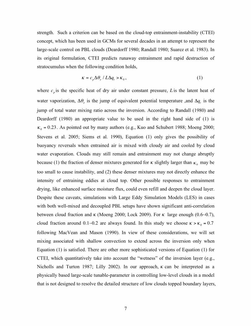
We performed in total four sets of GFS experiments as listed in Table 1. In these
experiments, we used a T126 version of the model and version 2 of the Relaxed
Arakawa-Schubert (Moorthi and Suarez 1992, 1999) parameterization for the deep
convection scheme. Observed SST was prescribed in the boundary conditions in all four
experiments. Simulations started at 00 UTC June 13th and ended at 00 UTC August 5th,
2008. Monthly means in July are used in this study. Analyses are mainly focused in the
region of Equator-40S, 110W-70W, which we will refer to as the SEP in the remainder of
this paper.
i. The CONTROL experiment was done with the operational treatment of shallow
convection and background diffusion.
ii. Experiment CTEI is the same as the CONTROL, except that the definition of the
inversion and the criterion for instability expressed by Equation 1 are
incorporated.
iii. Experiment ZEROBD sets the background diffusion to 0 in layers above the
inversion layer.
iv. Experiment CZ has both the CTEI and the ZEROBD modifications.
Table 1: List of experiments performed in this study
9
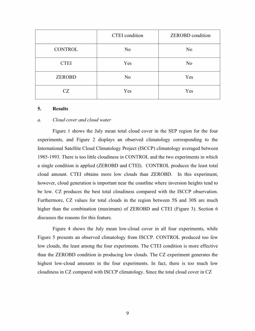
5. Results
a. Cloud cover and cloud water
Figure 1 shows the July mean total cloud cover in the SEP region for the four
experiments, and Figure 2 displays an observed climatology corresponding to the
International Satellite Cloud Climatology Project (ISCCP) climatology averaged between
1985-1993. There is too little cloudiness in CONTROL and the two experiments in which
a single condition is applied (ZEROBD and CTEI). CONTROL produces the least total
cloud amount. CTEI obtains more low clouds than ZEROBD. In this experiment,
however, cloud generation is important near the coastline where inversion heights tend to
be low. CZ produces the best total cloudiness compared with the ISCCP observation.
Furthermore, CZ values for total clouds in the region between 5S and 30S are much
higher than the combination (maximum) of ZEROBD and CTEI (Figure 3). Section 6
discusses the reasons for this feature.
Figure 4 shows the July mean low-cloud cover in all four experiments, while
Figure 5 presents an observed climatology from ISCCP. CONTROL produced too few
low clouds, the least among the four experiments. The CTEI condition is more effective
than the ZEROBD condition in producing low clouds. The CZ experiment generates the
highest low-cloud amounts in the four experiments. In fact, there is too much low
cloudiness in CZ compared with ISCCP climatology. Since the total cloud cover in CZ
CTEI condition ZEROBD condition
CONTROL No No
CTEI Yes No
ZEROBD No Yes
CZ Yes Yes

10
Figure 1. The July 2008 mean total cloud cover in the SEP region in all four experiments.
Figure 2. The ISCCP July mean (1985-1993) total cloudiness in July in the SEP
region

11
Figure 3. The combined monthly mean total clouds from ZEROBD and CTEI in
July 2008 in the SEP region (not a necessary figure)
Figure 4. As in Fig. 1 except for low clouds

12
is about the same as in the ISCCP climatology, this result suggests a mismatch between
the simulated cloud types in CZ and those in the ISCCP climatology. There may be many
reasons for this mismatch. One obvious reason is the different low cloud definitions in
the GFS and in ISCCP. Clouds from 1000 mb to 680 mb are considered low clouds in
ISCCP, while in the GFS low clouds are below 642 mb. Another reason is that ISCCP
tends to underestimate low-cloud cover (Chang and Li, 2005; Comments also made by
Dr. Chris Fairall at the Second VOCAL meeting in Seattle, 2009). A comparison between
Figure 1 and Figure 4 shows that the most of the total clouds in CZ are from low clouds.
Figure 6 shows examples of the vertical structures of cloud water in SEP along
20S. Most of the cloud water produced in the CONTROL is located off the coast. Both
the CTEI and ZEROBD experiments generated more cloud water near the coast and at
low levels than the CONTROL. The CZ experiment generated the most cloud water,
especially at lower levels, much more than the combined amount from both the CTEI and
ZEROBD experiments. This is consistent with the fact that vertical diffusion processes in
the CONTROL experiment are strong, while CZ allows for mixing across the inversion
only when CTEI exists.
b. Radiation
Radiative fluxes at the surface and the top of the atmosphere in the simulations
are examined and compared with the corresponding flux climatology averaged between
1984-1994 compiled by the Surface Radiation Budget (SRB) project (http://GEWEX-
SRB.larc.nasa.gov/). Since data on cloud amount from ISCCP were used to build the
SRB dataset, some degree of consistency between the two datasets are expected. Figure 7
shows the 2008 July mean short-wave radiative flux errors at the surface defined as the
differences between the simulated values in the four experiments and the observed
climatology from SRB. The short-wave radiative flux at the surface is mostly larger in
the CONTROL, ZEROBD, and CTEI experiments than the observed value in SRB,
consistent with less cloudiness than the observed climatology in ISCCP. The short-wave

13
Figure 5. As in Fig 2 except for low clouds
Figure 6. Vertical cross-section of monthly mean cloud water in July along 20S.

14
radiative flux at the surface in CZ is smaller than that in SRB in most of the VOCALS
region (except for the portion near the coast) due to more clouds generated in the
simulation than the climatology. It should be pointed out that either tuning the
microphysics, the shortwave parameterization, or the CTEI tunable parameter could
alleviate the excessive absorption of shortwave. It is a known fact that the shortwave
parameterization used in this version of GFS absorbs too much shortwave radiation (Y.
Hou, personal communication). In terms of the downward long-wave radiative flux at the
surface, CZ is much better than the other three simulations shown in Figure 8. The
difference in long-wave radiative flux at the surface between CZ and the SRB
climatology is small, except near the coastal region. In the other 3 simulations, the long-
wave radiative fluxes at the surface are mostly smaller than the climatology due to the
shortage of low clouds. Figure 9 shows the July 2008 mean upward radiative flux errors
at the top of the atmosphere (TOA). The radiative fluxes at the TOA also reflect the
cloudiness generated in the simulations. More upward short-wave radiative flux is
produced at the TOA in CZ than in the other three simulations because the latter produces
more cloudiness. Compared with the SRB climatology, the upward short-wave radiative
flux away from the coast at the TOA is too large in CZ and too small in the other three
simulations. The outgoing long wave radiation (OLR) errors at the TOA are illustrated in
Figure 10. Values of OLR are large in all simulations compared with the observations.
The differences in OLR between CZ and the SRB climatology are smallest.
c. Surface winds and latent heat flux
Figure 11 shows surface winds in the four experiments. From the equator
southward, all experiments show the transition between low-latitude trades and mid-
latitude westerlies. A striking difference among the four experiments is the strength of the
trade winds. Trade winds in the ZEROBD and in the CZ experiments especially near the
coast are stronger than in the CONTROL, while the trade winds are smaller in the CTEI.
The width of the transition region and the strength of the westerlies are also very different

15
Figure 7. The July 2008 mean surface downward shortwave radiative flux errors
(difference between the four simulations and SRB climatology)
Figure 8. As in Fig. 7 except for longwave radiative flux errors

16
Figure 9. The July 2008 mean upward shortwave radiative flux errors (difference
between the simulations and SRB climatology) at the top of the atmosphere in the
four experiments.
Figure 10. As in Fig.9 except for the longwave radiative flux errors

17
among the experiments. The transition regions are larger and westerlies are weaker in CZ
and CTEI than in CONTROL and ZEROBD. The transition region is smallest and
westerlies are strongest in ZEROBD while the opposite is true for CTEI. Figure 12
shows the latent heat fluxes in the four experiments. To some degree the latent heat fluxes
reflect the wind intensity. For instance, in the trade wind region, the latent heat flux is
largest in CZ corresponding to the strongest winds. However, wind alone does not
determine the latent heat flux. The latent heat fluxes are smaller in CZ between 35 S and
40 S than that in CTEI despite the stronger winds in CZ, which indicates that the
moisture difference between the sea surface and the air above is smaller in CZ than in
CTEI.
Figure 11. The July 2008 mean surface wind magnitude (shaded ms-1) and direction
(arrows) in the four experiments.

18
Figure 12. The July 2008 mean surface latent heat flux (W m2) in the four experiments
6. Relative impact of ZEROBD and CTEI conditions
The shallow convection scheme in the GFS acts through enhanced diffusion in the
cloudy layers. The scheme warms and dries the lower layers and cools and moistens the
upper layers. Figure 13 shows vertical cross-sections of monthly mean moistening rates
along 20S from 110W to 70W due to shallow convection in the four experiments. Mixing
is the most intense in CONTROL and the least intense in CZ. Mixing in CTEI is weaker
than that in ZEROBD. The mixing layers in CONTROL and ZEROBD are thicker than in
CTEI and CZ. We surmise that the lower amount of mixing in CZ is the main reason for
the greater cloudiness in the experiment. Due to less mixing, more moisture is trapped at
low levels in CZ than in the other three experiments. Then, the large-scale condensation
(microphysical process) and, to a certain extent, RAS, take over to produce more clouds.
The ZEROBD experiment does not directly reduce mixing due to shallow convection.
But, by reducing background mixing, it tends to increase the strength of the inversion,
which then reduces the chance of shallow convection activity by decreasing convective
available potential energy (CAPE). When combined with CTEI in CZ, this increase in the

19
strength of the inversion due to ZEROBD probably has an additional impact. With a
stronger inversion, the CTEI condition tends to allow less shallow convection activity
according to Eq. (1). Figure 14 shows the monthly mean vertical cross-sections of heating
rate (shaded) due to large-scale condensation/evaporation and temperature (contours)
along 20S in the four experiments. Positive heating rate (warming) due to large-scale
condensation is only found in CZ. Negative heating rates (cooling) in the other three
experiments and at low levels in CZ are due to the evaporation of cloud and rainwater.
The most intense warming in CZ happened roughly below the inversion (inversion height
changes with longitude and with time), which is where most clouds are produced. The
RAS also produces clouds through detrainment of cloud water at the cloud top. Figure 15
illustrates the convective heating rate due to RAS, where the RAS is most active in CZ
and is more active in CTEI than in CONTROL or ZEROBD. Since large-scale
condensation did not help to produce clouds in CONTROL, ZEROBD, and CTEI, it was
RAS that produced clouds through detrainment in these experiments. Clouds in CZ are
generated both through RAS and in-situ large-scale condensation. Reduced moisture
diffusion under the inversion allows for increased relative humidity leading to large-scale
condensation below inversion. The RAS also provides more moisture near the inversion
through detrainment, which results in large-scale condensation. However, large-scale
condensation is the main process producing the clouds. Figure 16 illustrates the vertical
cross-sections of heating rates due to large-scale condensation overlaid with cloud water
mixing ratios. In Figure 16 the most dramatic heating rates occur in the region of the
most cloud water. Besides producing clouds by detraining cloud water at the cloud top,
RAS also indirectly contributes to the cloud production in CZ by reducing mixing by
shallow convection. This is because shallow convection is shut off whenever RAS is
activated unless the cloud depth is less than 200 hPa.
7. Impacts on global precipitation
Figure 17 shows the July 2008 mean global precipitation rate (mm/day) in the
four experiments. The Climate Prediction Center (CPC) Merged Analysis of Precipitation
(CMAP; Xie and Arkin, 1996) climatology averaged between 1979-2005 is shown in
Figure 18. Compared with CONTROL, the other three experiments produce more

20
Figure 13. Vertical cross-sections of monthly mean moistening rates (g/kg/day)
along 20S in shades due to shallow convection in the four experiments. Contours
represent vertical cross-section of temperature.
Figure 14. As in Fig. 13 except for the heating rate (K/day) (shaded) due to large-
scale condensation.

21
Figure 15. As in Fig. 13 except for convective heating rate (K/day) due to RAS
Figure 16. Vertical cross-sections of monthly mean heating rate due to large-scale
condensation (K/day) along 20S in shades overlaid with monthly mean cloud
water mixing ratios (g/kg) in contours

22
precipitation over the western Pacific warm pool and maritime continental area and less
precipitation over the eastern Pacific ITCZ. The CZ produces the most precipitation in
the west Pacific and least in the east Pacific among all four experiments. The
precipitation rate is smaller in the southern pacific convergence zone (SPCZ) and larger
in the mid-Pacific ITCZ in CZ than in the CONTROL. An interesting feature that occurs
only in CZ is the 1-2 mm/day precipitation rate in the SEP region. This light precipitation
is primarily caused by large-scale processes. In reality, this is the region where drizzle
occurs. Compared with the CMAP climatology most of the main precipitation features
are produced in the four experiments, for instance, rain bands associated with the ITCZ,
SPCZ, the mid-latitude oceanic storm tracks, and the tropical continental maxima. The
precipitation intensities in these regions from the experiments differ from CMAP in that
too much precipitation is produced over the western warm pool and the east tropical
Pacific. The ITCZ in the four experiments are narrower than in CMAP. Since
precipitation in the simulations are only one-month means and the CMAP precipitation is
monthly means averaged over many years, the differences in precipitation intensity and
the width of the ITCZ between the simulations and CMAP may not be surprising.
8. Summary
Several methods have been tested in the NCEP GFS model to alleviate an
important systematic error: the lack of stratocumulus in the SEP region. This paper
described two simple modifications: (a) elimination of background vertical diffusion
above the low-level inversion (ZEROBD), and (b) incorporation of a tunable parameter
based on the CTEI criterion for determining cloud tops for the shallow convection
parameterization when low-level inversions exist (CTEI). Four simulations were
performed to examine the individual effect of each modification and the combined effect
of the two modifications on the generation of the stratocumulus clouds. Both
modifications enhanced clouds generation in the SEP region. The CTEI is more effective
than ZEROBD in producing low-level clouds. However, ZEROBD is also shown to be
important, especially close to the coast. A comparison with the ISCCP climatology
reveals that both modifications individually produced too little cloudiness. However, the

23
two modifications applied together produced about the right amount of total cloudiness in
the region. The combination is much more effective than any of the two modifications
alone. The reason for this nonlinearity is that both changes reinforce each other in
reducing the leakage of moisture across the inversion. Less mixing traps more moisture in
lower levels below the inversion and results in more condensation. This enhanced
response in the combined case also implies that the effectiveness of the CTEI-based
algorithm depends sensitively on the strength of the inversion. In generating clouds the
large-scale condensation process was the main contributor. The RAS scheme also
provided a positive, but small contribution. Although roughly of the correct magnitude,
the amount of total cloudiness obtained in the simulation with both modifications may
produce different low, middle, and high cloud amounts than the observations. The
availability of reliable observations of the vertical distribution of cloud water will be very
helpful for verifying climate models. The impacts of this mismatch on the coupled
climate system simulation have yet to be studied.
Figure 17 The July 2008 mean precipitation rate (mm / day) in the four experiments.

24
Figure 18. The global July mean CMAP precipitation rate (mm/day) averaged
between 1979 and 2005 ( Xie and Arkin, 1997 )
Our experiments have demonstrated that it is possible to simulate realistic marine
boundary clouds in large-scale models with relatively simple and physically based
changes in the major model parameterizations. Although the CZ experiment may have
produced too much cloud cover or too much cloud water, it is possible to further improve
these fields by slightly modifying the microphysics, and/or cloudiness parameterizations,
and/or the CTEI tunable parameter. This should also reduce the excessive reduction of
shortwave radiation at the ocean surface. NCEP is currently moving towards
implementing in its operational models the RRTM shortwave radiation parameterization
with maximum/random overlap. This radiation scheme has less shortwave absorption in
the clouds, which together with a slightly tuned microphysics should further improve the
surface shortwave radiation at the ocean surface. At the present time, the two
modifications presented in this paper have been implemented in the model in the new
CFS reanalysis (Saha et al., 2010).
Acknowledgements: This project is supported by NOAA NA07OAR4310236. SRB data were obtained from the NASA Langley Research Center Atmospheric Sciences Data Center NASA/GEWEX SRB Project. We would like to thank Dr. Huiya Chuang for her help with the d3d analysis and Drs. Hualu Pan, Jongil Han, and others at EMC for their

25
generous help with the GFS/CFS. We appreciate helpful comments from Drs. Brad Ferrier and Glenn White during the internal review process.
REFERENCES Alpert, J.C., 2004: subgrid-scale mountain blocking at NCEP. Proc. Of 20th conf. on
Weather and Forecasting, Seatle, WA.
Bony, S. and J.-L.Dufresre, 2005: Marine boundary layer clouds at the heart of tropical
cloud feedback uncertainties in climate models, Geopys. Res. Lett., 32, L20806,
doi:10.1029/2005GL023851
Chang, F. and Z. Li, 2005: A near-global climatology of single-layer and overlapped
clouds and their optical properties retrieved from Terra/MODIS data using a new
algorithm, J. Climate, 18, 4752-4771
Chou, M.D, M. J. Suarez, C. H. Ho, M. M. H. Yan, and K. T. Lee, 1998:
Parameterizations of cloud overlapping and shortwave single scattering properties for
use in general circulation and cloud ensemble models. J. Climate, 11, 202-214
Deardorff, J.W., 1980: cloud top entrainment instability, J. Atmos. Sci., 37, 131-147
Hannay, C., D.L. Williamson, J.J. Hack, J.T. Kiehl, J.G. Olson, S.A. Klein, C.S.
Bretherton, and M. Köhler, 2009: Evaluation of Forecasted Southeast Pacific
Stratocumulus in the NCAR, GFDL, and ECMWF Models. J. Climate, 22, 2871–
2889.
de Szoeke, S.P., Y. Wang, S.-P. Xie, and T. Miyama, 2006: Effect of shallow cumulus
convection on the eastern Pacific climate in a coupled model. Geophys. Res. Lett., 33,
L17713, doi:10.1029/2006GL026715
Ek M.B., K.E. Mitchell, Y. Lin, E. Rogers, P. Grummann, V. Koren, G. Gayno, and J.D.
Tarplay, 2003: Implementation of the Noah land-use model advances in the NCEP
operational mesoscale Eta model. J. Geophys. Res. 108 , 8851,
doi:10.1029/2002JD003296
Gordon, C.T., A. Rosati, and R. Gudgel, 2000: Tropical sensitivity of a coupled model to
specificed ISCCP low clouds. J. Climate, 13, 2239-2260
Hong, S. -Y. and H. -L. Pan, 1996: Nonlocal boundary layer vertical diffusion in a

26
medium range forecast model. Mon. Wea. Rev., 124, 2322-2339.
Hong, S. -Y. and H. -L. Pan, 1998: Convective Trigger Function for a Mass-Flux
Cumulus Parameterization Scheme. Mon. Wea. Rev., 126, 2599–2620.
Hou, Y. -T., K. A. Campana and S.–K. Yang, 1996: Shortwave radiation calculations in
the NCEP's global model. Int. Radiation Symposium, IRS-96, August 19-24,
Fairbanks, AL.
Hou, Y., S. Moorthi, and K. Campana, 2002: Parameterization of solar radiation transfer
in the NCEP models. NCEP Office Note, 441.
http://www.emc.ncep.noaa.gov/officenotes/FullTOC.html#2000.
Kalnay, E. and Coauthors, 1996: The NCEP/NCAR 40-year Reanalysis Project. Bull.
Amer. Meteor. Soc., 77, 1057-1072.
Klein, S.A., and D.L. Hartmann, 1993: The seasonal cycle of low stratiform clouds. J.
Climate, 6, 1587-1606.
Kollias, P., C.W. Fairall, P. Zuidema, J. Tomlinson, and G.A. Wick, 2004: Observations
of marine stratocumulus in SE Pacific during the PACS 2003 cruise. Geophs. Res.
Lett., 31 , L22110
Kuo, H., and W.H. Schubert, 1988: Stability of cloud-topped boundary layers. Quart. J.
Roy. Meteor. Soc., 114, 887–917.
Lock, A.P., 2009: Factors influencing cloud area at the capping inversion for shallow
cumulus clouds. Quart. J. Roy. Meteor. Soc 135(641): 941
Lilly, D.K., 2002: Entrainment into mixed layers. Part III: A new closure. J. Atmos. Sci.,
59, 3353-3361
Lott, F. and M. J. Miller, 1997: A new subgrid-scale orographic drag parameterization:
Its performance and testing. Quart. J. Roy. Meteor. Soc., 123, 101-127
Ma, C.-C., C.R. Mechoso, A.W. Robertson and A. Arakawa, 1996: Peruvian stratus
clouds and the tropical Pacific circulation: A coupled ocean-atmosphere GCM study.
J. Climate, 9, 1635-1645.
MacVean, M.K., and P.J. Mason, 1990: Cloud-top entrainment instability through small-

27
scale mixing and its parmeterization in numerical models. J. Atmos. Sci., 47, 1012-1030
Mechoso, C.R., and coauthors, 1995: The seasonal cycle over the tropical Pacific in
coupled ocean-atmosphere general circulation models. Mon. Wea. Rev., 123, 2825-
283
Mechoso, C.R. and coauthors, 2005: VAMOS Ocean-Cloud Atmosphere-Land Study
(VOCALS) Science Paln, 42 PP. [Available online at
http:www.eol.ucar.edu/projects/vocals/science_planning/VOCALS-Science-Plan.pdf]
Mlawer E. J., S. J. Taubman, P. D. Brown, M.J. Iacono and S.A. Clough, 1997: radiative
transfer for inhomogeneous atmosphere: RRTM, a validated correlated-K model for
the longwave. J. Geophys. Res., 102(D14), 16,663-16,6832.
Moeng C.-H., 2000: Entrainment rate, cloud fraction and liquid water path of PBL
stratocumulus clouds. J. Atmos. Sci., 57, 3627–3643
Moorthi, S., and M. J. Suarez, 1992: Relaxed Arakawa-Schubert. A Parameterization of
Moist Convection for General Circulation Models. Mon. Wea. Rev., 120, 978- 1002.
Moorthi, S., and M. J. Saurez, 1999: Documentation of version 2 of Relaxed Arakawa-
Schubert cumulus parameterization with convective downdrafts. NOAA Tech. Report
NWS/NCEP 99-01, 44pp
Moorthi, S., H. L. Pan and P. Caplan, 2001: Changes to the 2001 NCEP operational
MRF/AVN global analysis/forecast system. NWS Technical Procedures Bulletin, 484,
pp14. [Available at http://www.nws.noaa.gov/om/tpb/484.htm]
Nicholls S.k and J.D. Turton, 1986: an observational study of the stracture of stratiform
cloud streets. Art II: Entrainment. Quart. J. Roy. Meteor. Soc., 112, 461-480
Pan, H.-L. and W.-S. Wu, 1995: implementing a mass flux convective parameterization
package for the NMC medium range forecast model. NMC office note 409, 40
PP.[Available online at
http://www.emc.ncep.noaa.gov/officenotes/FullTOC.html#1990]
Randall, D. A., 1980: conditional instability of the first kind upside-down. J. Atmos. Sci,
37, 125-130
Saha, S. and Coauthors, 2006: The NCEP climate forecast system, J. Climate, 19, 3483-
3517

28
Saha, S., and Coauthors, 2010: The NCEP climate forecast system reanalysis. Submitted
to Bull. Amer. Met. Soc.
Sela, 2009: Implementation of the sigma pressure hybrid coordinate into GFS. NCEP
office Note # 461[available at
http://wwww.emc.ncep.noaa.gov/officenotes/FullTOC.html#2000].
Siems, S.T., C.S. Bretherton, M.B. Baker, S.S. Shy, and R.E. Breidenthal,1990:
Buoyancy reversal and cloud-top entrainment instability.Quart. Quart. J. Roy.
Meteor. Soc., 116, 705–739.
Stevens, B., C.H. Moeng, A.S. Ackerman, C.S. Bretherton, A. Chlond, S. de Roode, J.
Edwards, J.C. Golaz, H. Jiang, M. Khairoutdinov, M.P. Kirkpatrick, D.C. Lewellen,
A. Lock, F. Müller, D.E. Stevens, E. Whelan, and P. Zhu, 2005: Evaluation of Large-
Eddy Simulations via Observations of Nocturnal Marine Stratocumulus. Mon. Wea.
Rev., 133, 1443–1462.
Sundqvist, H., E. Berge, and J. E. Kristjansson, 1989: Condensation and cloud studies
with mesoscale numerical weather prediction model. Mon. Wea. Rev., 117, 1641-
1757.
Tiedtke, M., 1983: The sensitivity of the time-mean large-scale flow to cumulus
convection in the ECMWF model. ECMWF Workshop on Convection in Large-Scale
Models, 28 November – 1 December 1983, Reading, England, pp. 297-316.
Wang, W., S. Saha, H.-L. Pan, S. Nadiga, G. White, 2005: Simulation of ENSO in the
new NCEP coupled forecast system model (CFS03), Mon. Wea. Rev., 133, 1574-1593
Wang, Y., H. Xu, and S.P. Xie, 2004: Regional model simulations of marine boundary
layer clouds over the southeast Pacific off South America. Part II: sensitivity
experiments. Mon. Wea. Rev.,132, 2650-2668
Xie, P., and P.A. Arkin, 1997: Global precipitation: a 17-year monthly analysis based on
gauge observation, satellite estimates, and numerical model outputs. Mon, Wea. Rev.,
78, 2539-2558.
Xu, K.M., and D.A. Randall, 1996: A semiemperical cloudiness parameterization for use
in climate models. J. Atmos. Sci., 53, 3084-3102
Zhao, Q. Y., and F. H. Carr, 1997: A prognostic cloud scheme for operational NWP
models. Mon. Wea. Rev., 125, 1931-1953.