“South Texas Eagle Ford and Olmos – from … Energy Presentation October 2010(2).pdf“South...

30 Years of Seizing Opportunities

1979 – 2009

2010 TIPRO Central Texas Business Development Reception

October 20, 2010

“South Texas Eagle Ford and Olmos –from Unconventional to

Conventional”

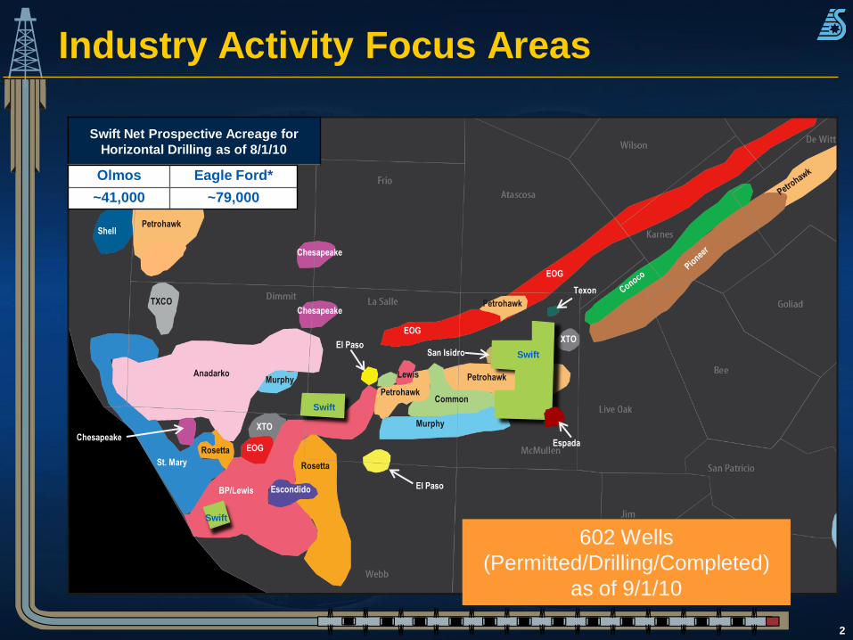
Industry Activity Focus Areas

2

Petrohawk

Petrohawk

Petrohawk

Anadarko

EOG

EOG

EOG

XTO

XTO

Escondido

Murphy

Murphy

Common

BP/Lewis

Lewis

St. Mary

Chesapeake

Chesapeake

Chesapeake

TXCO

Shell

Espada

San Isidro

Texon

Rosetta

Rosetta

Petrohawk

El Paso

El Paso

602 Wells

(Permitted/Drilling/Completed)

as of 9/1/10

Swift

Swift

Swift

Swift Net Prospective Acreage for

Horizontal Drilling as of 8/1/10

Olmos Eagle Ford*

~41,000 ~79,000

3

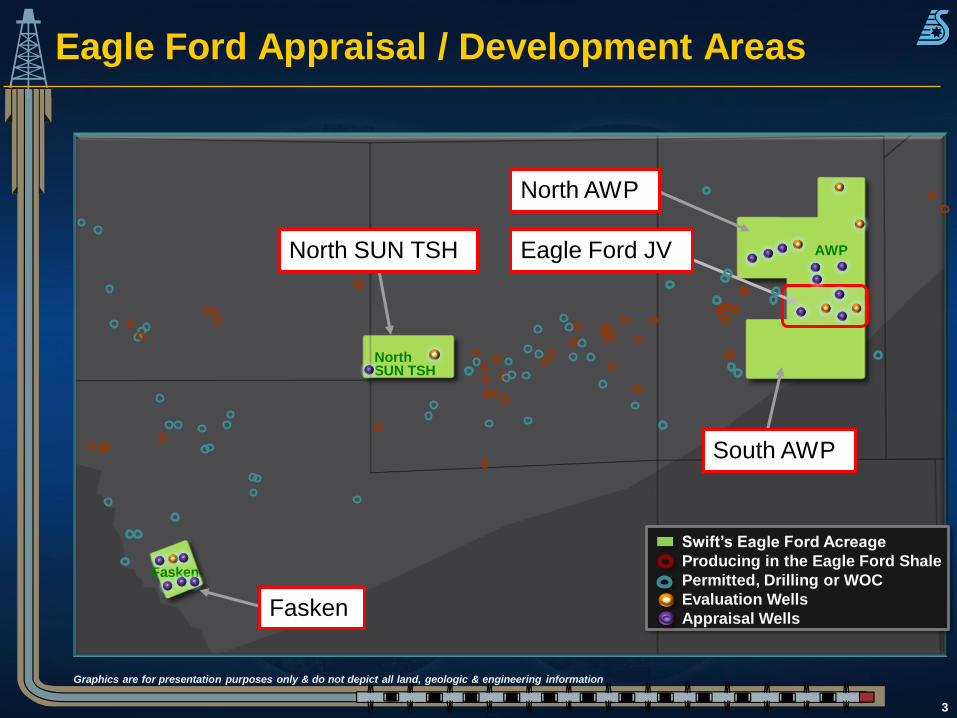
Eagle Ford Appraisal / Development Areas

Fasken

North SUN TSH

North AWP

Eagle Ford JV

South AWP

Fasken

North SUN TSH

AWP

Graphics are for presentation purposes only & do not depict all land, geologic & engineering information

Swift’s Eagle Ford Acreage

Producing in the Eagle Ford Shale

Permitted, Drilling or WOC

Evaluation Wells

Appraisal Wells

4

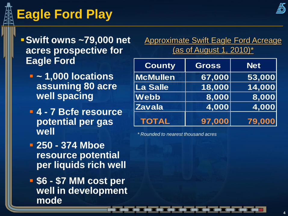
Eagle Ford Play

Approximate Swift Eagle Ford Acreage

(as of August 1, 2010)*

* Rounded to nearest thousand acres

Swift owns ~79,000 net acres prospective for Eagle Ford

~ 1,000 locations assuming 80 acre well spacing

4 - 7 Bcfe resource potential per gas well

250 - 374 Mboe resource potential per liquids rich well

$6 - $7 MM cost per well in development mode

County Gross Net

McMullen 67,000 53,000

La Salle 18,000 14,000

Webb 8,000 8,000

Zavala 4,000 4,000

TOTAL 97,000 79,000

5

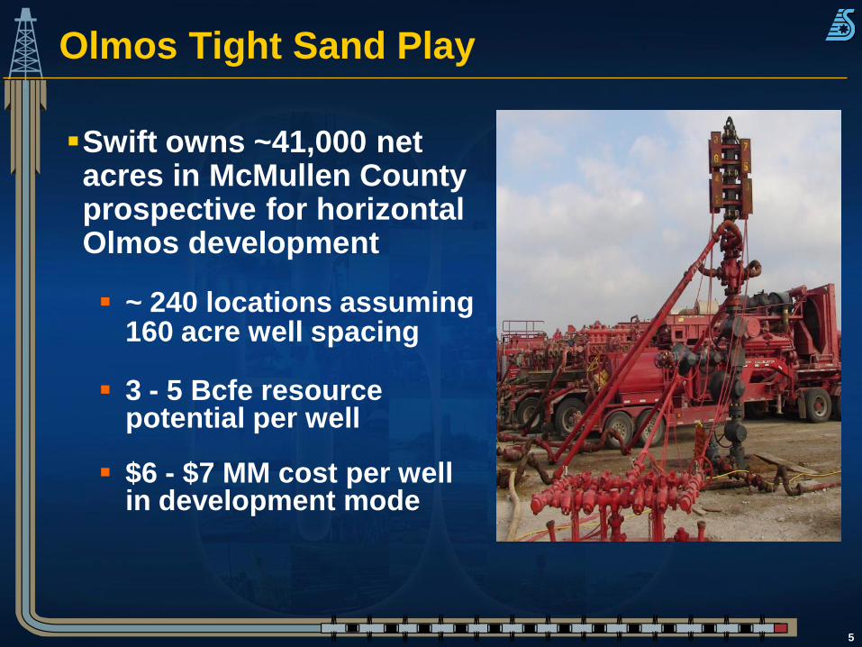
Olmos Tight Sand Play

Swift owns ~41,000 net acres in McMullen County prospective for horizontal Olmos development

~ 240 locations assuming 160 acre well spacing

3 - 5 Bcfe resource potential per well

$6 - $7 MM cost per well in development mode

6

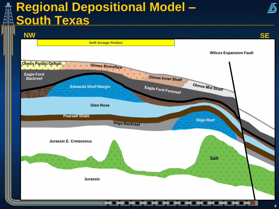
NW SE

Jurassic

Salt

Sligo Reef

Edwards Shelf Margin

Glen Rose

Eagle FordBackreef

Pearsall Shale

Olmos Paralic-Deltaic

Jurassic E. Cretaceous

Wilcox Expansion Fault

Swift Acreage Position

Regional Depositional Model –South Texas

7

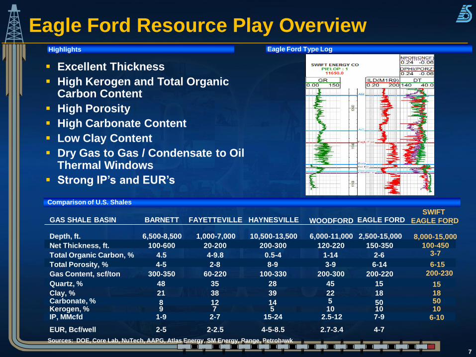
Eagle Ford Resource Play Overview

GAS SHALE BASIN BARNETT FAYETTEVILLE HAYNESVILLE WOODFORD EAGLE FORD

Depth, ft. 6,500-8,500 1,000-7,000 10,500-13,500 6,000-11,000 2,500-15,000

Net Thickness, ft. 100-600 20-200 200-300 120-220 150-350

Total Organic Carbon, % 4.5 4-9.8 0.5-4 1-14 2-6

Total Porosity, % 4-5 2-8 8-9 3-9 6-14

Gas Content, scf/ton 300-350 60-220 100-330 200-300 200-220

Quartz, % 48 35 28 45 15

Clay, % 21 38 39 22 18Carbonate, % 8 12 14 5 50Kerogen, % 9 7 5 10 10

Sources: DOE, Core Lab, NuTech, AAPG, Atlas Energy, SM Energy, Range, Petrohawk

Comparison of U.S. Shales

Eagle Ford Type Log

Excellent Thickness

High Kerogen and Total Organic Carbon Content

High Porosity

High Carbonate Content

Low Clay Content

Dry Gas to Gas / Condensate to Oil Thermal Windows

Strong IP’s and EUR’s

Highlights

SWIFT

EAGLE FORD

8,000-15,000

100-4503-7

6-15

200-230

15

185010

IP, MMcfd 1-9 2-7 15-24 2.5-12 7-9

EUR, Bcf/well 2-5 2-2.5 4-5-8.5 2.7-3.4 4-7

6-10

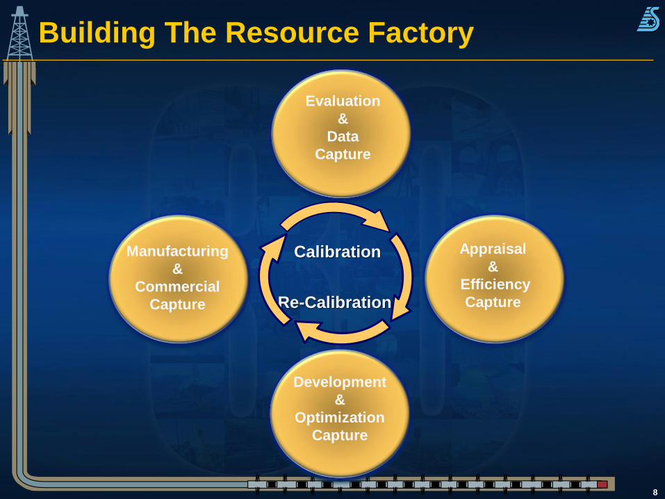
Building The Resource Factory

8

Manufacturing

&

Commercial

Capture

Evaluation

&

Data

Capture

Development

&

Optimization

Capture

Appraisal

&

Efficiency

Capture

Calibration

Re-Calibration

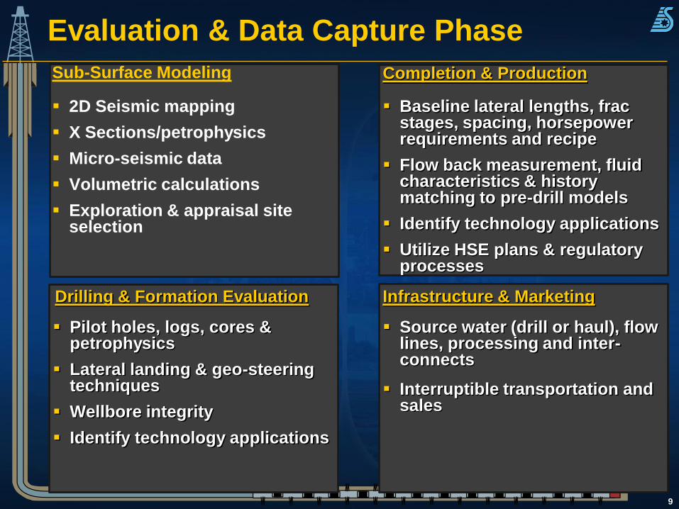
Evaluation & Data Capture Phase

9

Sub-Surface Modeling

2D Seismic mapping

X Sections/petrophysics

Micro-seismic data

Volumetric calculations

Exploration & appraisal site selection

Completion & Production

Baseline lateral lengths, frac stages, spacing, horsepower requirements and recipe

Flow back measurement, fluid characteristics & history matching to pre-drill models

Identify technology applications

Utilize HSE plans & regulatory processes

Infrastructure & Marketing

Source water (drill or haul), flow lines, processing and inter-connects

Interruptible transportation and sales

Drilling & Formation Evaluation

Pilot holes, logs, cores & petrophysics

Lateral landing & geo-steeringtechniques

Wellbore integrity

Identify technology applications

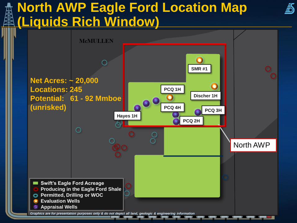
North AWP Eagle Ford Location Map (Liquids Rich Window)

North AWP


Net Acres: ~ 20,000

Locations: 245

Potential: 61 - 92 Mmboe

(unrisked)

SMR #1

Discher 1H

PCQ 1H




Evaluation Wells

Appraisal Wells

PCQ 2H

PCQ 3HPCQ 4H

Hayes 1H

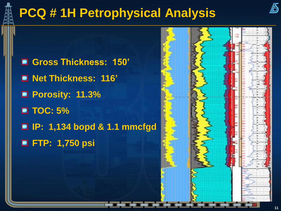
PCQ # 1H Petrophysical Analysis

11

Gross Thickness: 150’

Net Thickness: 116’

Porosity: 11.3%

TOC: 5%

IP: 1,134 bopd & 1.1 mmcfgd

FTP: 1,750 psi

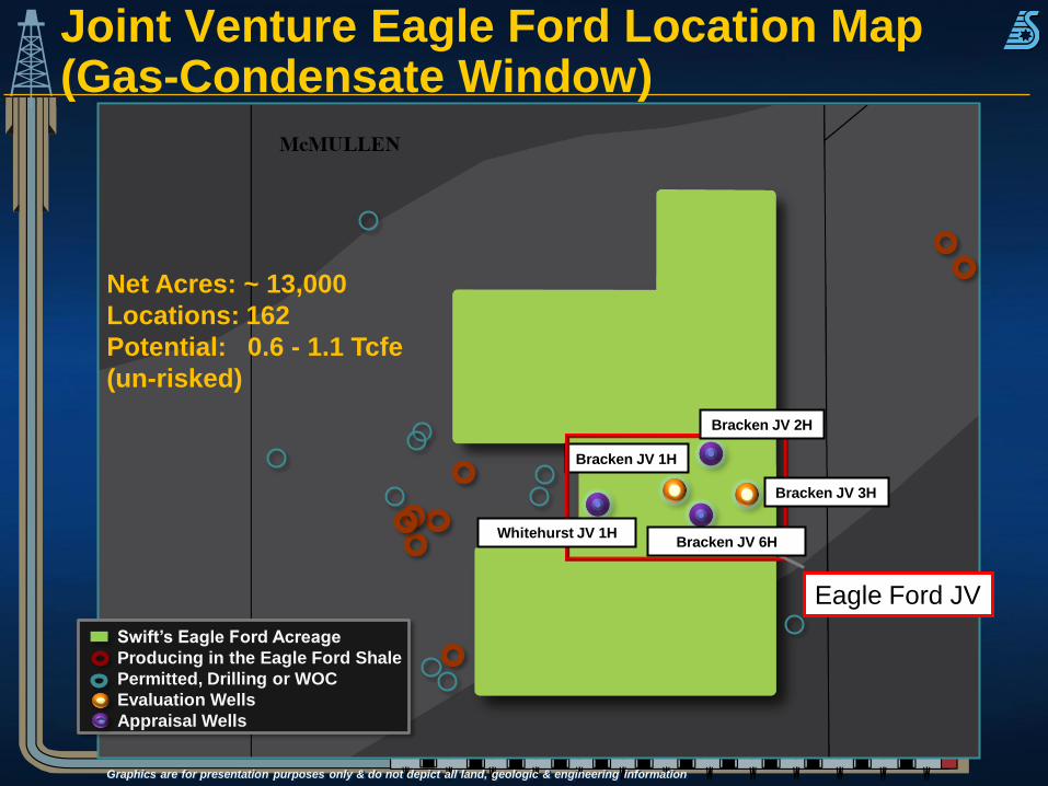
Eagle Ford JV

Bracken JV 1H


Joint Venture Eagle Ford Location Map (Gas-Condensate Window)

Net Acres: ~ 13,000

Locations: 162

Potential: 0.6 - 1.1 Tcfe

(un-risked)

Bracken JV 2H

Whitehurst JV 1H

Bracken JV 3H

Bracken JV 6H




Evaluation Wells

Appraisal Wells

13

BRACKEN- JV #3-HScale : 1 : 240

DEPTH (12700.FT - 13160.FT) 4/16/2010 08:53DB : Run 2 (1)

Lithology

GR (GAPI)0. 150.

RWA (Ohm-m)0. 0.1

PayFlag ()10. 0.

VWCL (Dec)0. 1.

Pay

VCL CO .35

Depth

DEPTH

(FT)

Zone

Cutoffs

Resistivity

A5VRM2W (Ohm-m)0.2 200.

A3VRM2W (Ohm-m)0.2 200.

Porosity

RHOB (g/cc)1.95 2.95

CNPOR (dec)0.45 -0.15

PHIE (Dec)0.45 -0.15

DFCAL (in)-20. 20.

Tight - Phie CO .06

Water

SW (Dec)0. 1.

BVW (Dec)0. 1.

Hig Water - Sw CO .55

Total Organic Content

TOCNeutron ()0. 20.

Gas

TotGasKB ()0. 1000.

ABSGasKB ()0. 1000.

Free Gas

Absorbed Gas

12750

12800

12850

12900

12950

13000

13050

13100

13150

Eagle

For

d

This zone is tight not wet

Lithology

GR (GAPI)0. 150.

RWA (Ohm-m)0. 0.1

PayFlag ()10. 0.

VWCL (Dec)0. 1.

Pay

VCL CO .35

Depth

DEPTH

(FT)

Zone

Cutoffs

Resistivity

A5VRM2W (Ohm-m)0.2 200.

A3VRM2W (Ohm-m)0.2 200.

Porosity

RHOB (g/cc)1.95 2.95

CNPOR (dec)0.45 -0.15

PHIE (Dec)0.45 -0.15

DFCAL (in)-20. 20.

Tight - Phie CO .06

Water

SW (Dec)0. 1.

BVW (Dec)0. 1.

Hig Water - Sw CO .55

Total Organic Content

TOCNeutron ()0. 20.

Gas

TotGasKB ()0. 1000.

ABSGasKB ()0. 1000.

Free Gas

Absorbed Gas

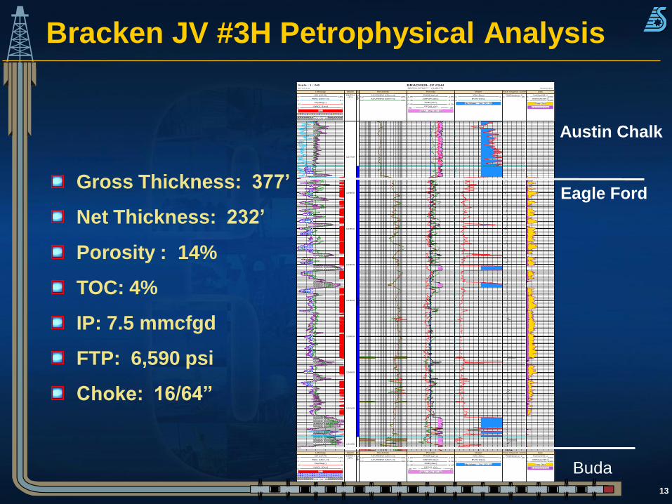
Eagle Ford

Buda

Austin Chalk



Porosity : 14%

TOC: 4%

IP: 7.5 mmcfgd

FTP: 6,590 psi

Choke: 16/64”

Bracken JV #3H Petrophysical Analysis

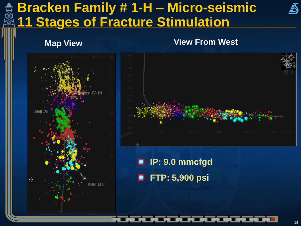
Bracken Family # 1-H – Micro-seismic11 Stages of Fracture Stimulation

14

Map View View From West

IP: 9.0 mmcfgd

FTP: 5,900 psi

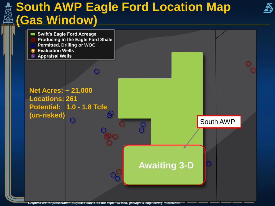
South AWP Eagle Ford Location Map(Gas Window)

Awaiting 3-D

South AWP


Net Acres: ~ 21,000

Locations: 261

Potential: 1.0 - 1.8 Tcfe

(un-risked)




Evaluation Wells

Appraisal Wells

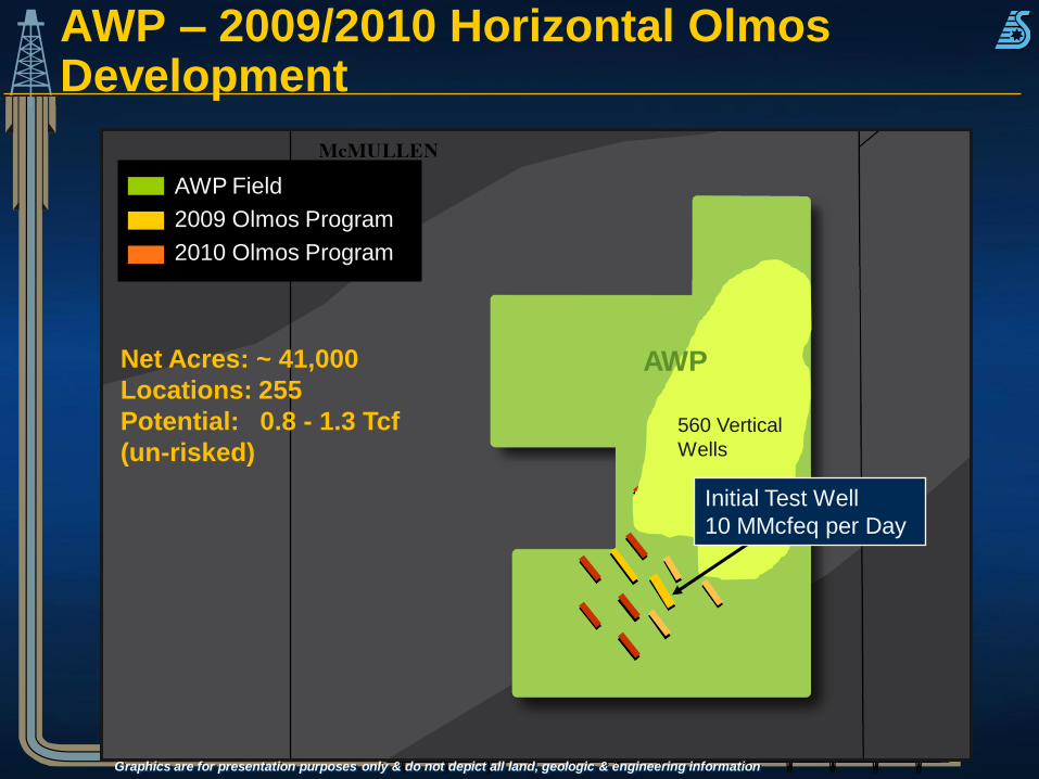
AWP – 2009/2010 Horizontal Olmos Development


AWP Field

2009 Olmos Program

2010 Olmos Program

Net Acres: ~ 41,000

Locations: 255

Potential: 0.8 - 1.3 Tcf

(un-risked)

AWP

Initial Test Well

10 MMcfeq per Day

560 Vertical

Wells

17

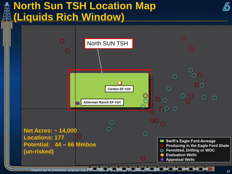
North Sun TSH Location Map(Liquids Rich Window)

North SUN TSH


Net Acres: ~ 14,000

Locations: 177

Potential: 44 – 66 Mmboe

(un-risked)




Evaluation Wells

Appraisal Wells

Carden EF #1H

Alderman Ranch EF #1H

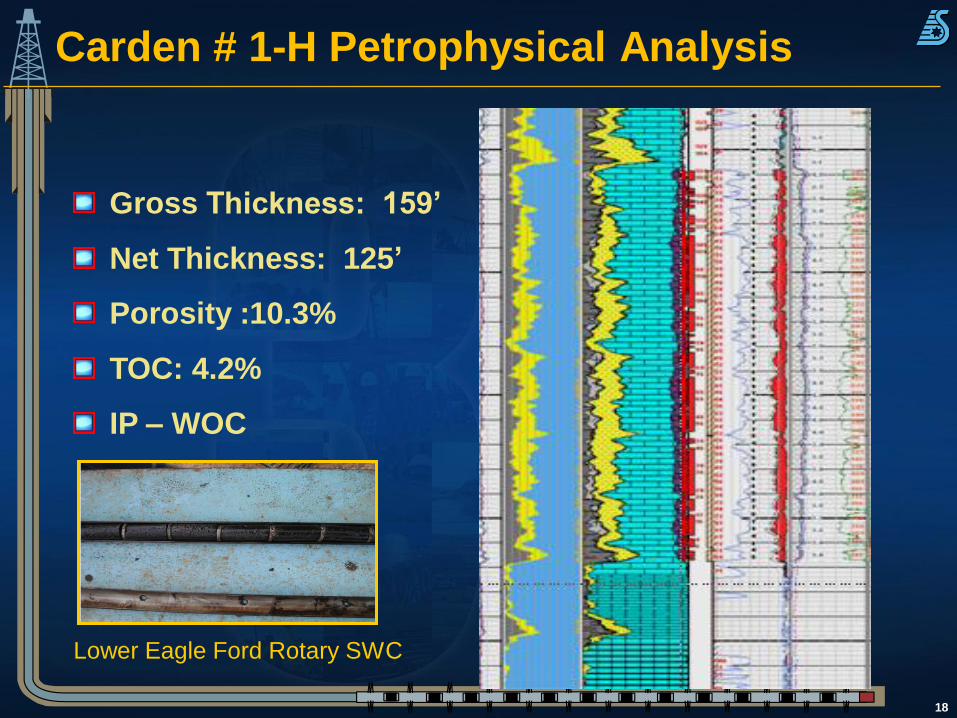
Carden # 1-H Petrophysical Analysis

18



Porosity :10.3%

TOC: 4.2%

IP – WOC

Lower Eagle Ford Rotary SWC

19

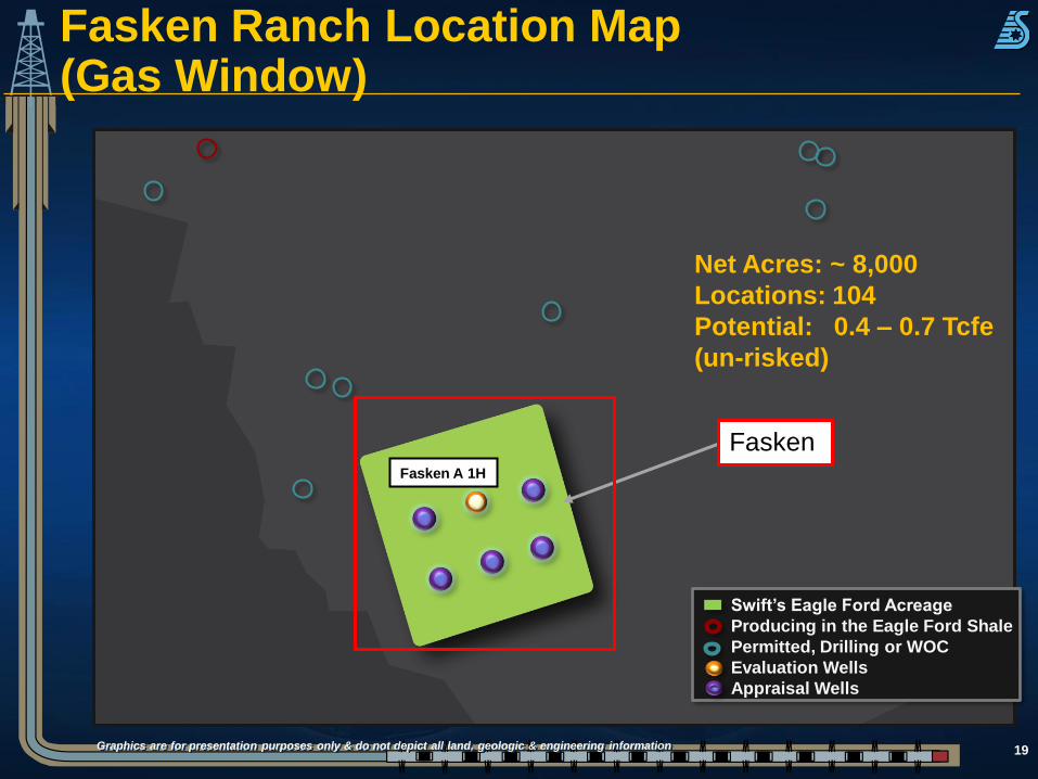
Fasken Ranch Location Map(Gas Window)

Fasken


Net Acres: ~ 8,000

Locations: 104

Potential: 0.4 – 0.7 Tcfe

(un-risked)




Evaluation Wells

Appraisal Wells

Fasken A 1H

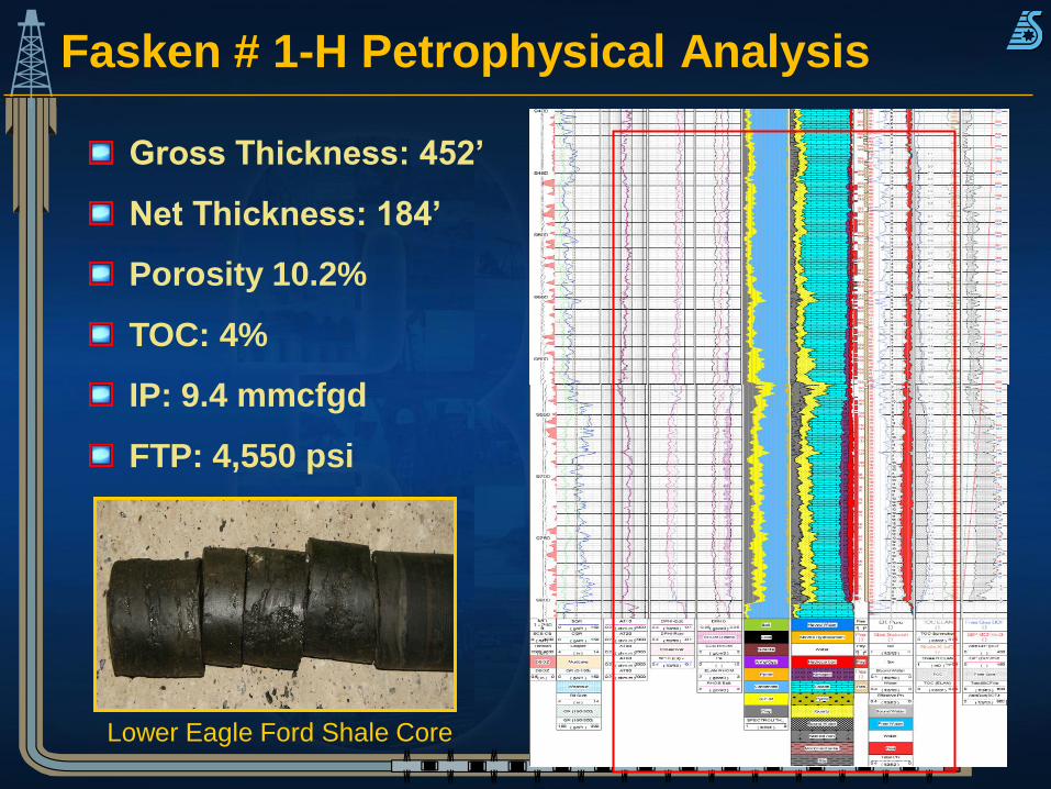
Fasken # 1-H Petrophysical Analysis

Lower Eagle Ford Shale Core



Porosity 10.2%

TOC: 4%

IP: 9.4 mmcfgd

FTP: 4,550 psi

21

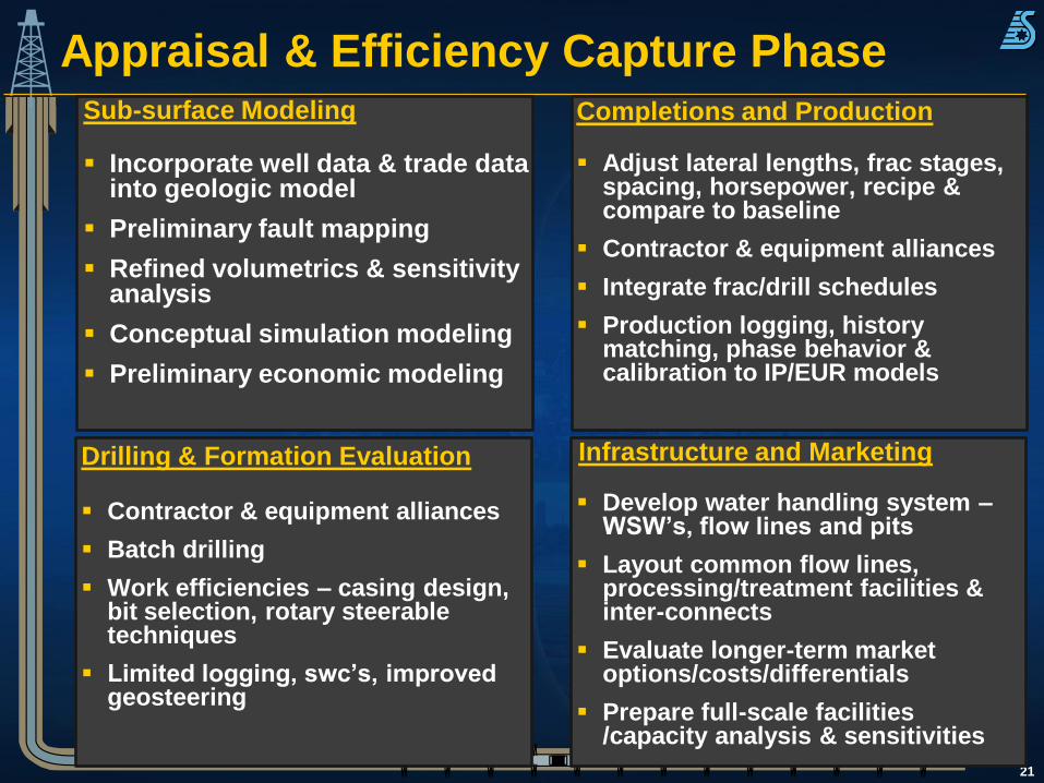
Sub-surface Modeling

Incorporate well data & trade data into geologic model

Preliminary fault mapping

Refined volumetrics & sensitivity analysis

Conceptual simulation modeling

Preliminary economic modeling

Drilling & Formation Evaluation

Contractor & equipment alliances

Batch drilling

Work efficiencies – casing design, bit selection, rotary steerable techniques

Limited logging, swc’s, improved geosteering

Appraisal & Efficiency Capture PhaseCompletions and Production

Adjust lateral lengths, frac stages, spacing, horsepower, recipe & compare to baseline

Contractor & equipment alliances

Integrate frac/drill schedules

Production logging, history matching, phase behavior & calibration to IP/EUR models

Infrastructure and Marketing

Develop water handling system –WSW’s, flow lines and pits

Layout common flow lines, processing/treatment facilities & inter-connects

Evaluate longer-term market options/costs/differentials

Prepare full-scale facilities /capacity analysis & sensitivities

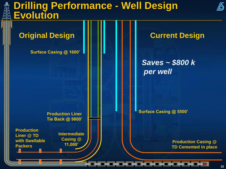
22

Production Liner

Tie Back @ 9800’

Production

Liner @ TD

with Swellable

Packers

Intermediate

Casing @

11,000’Production Casing @

TD Cemented in place

Drilling Performance - Well Design Evolution

Original Design Current Design

Surface Casing @ 1600’

Surface Casing @ 5500’

Saves ~ $800 k

per well

23

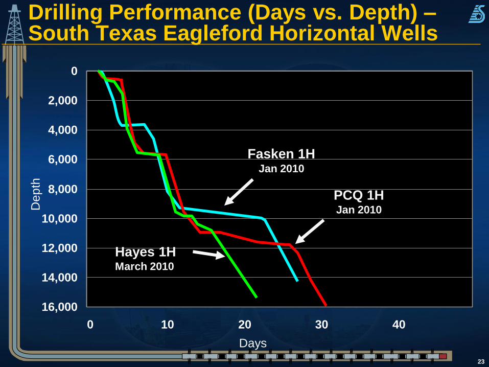
Drilling Performance (Days vs. Depth) –South Texas Eagleford Horizontal Wells

0

2,000

4,000

6,000

8,000

10,000

12,000

14,000

16,000

0 10 20 30 40

Fasken 1HJan 2010

PCQ 1HJan 2010D

ep

th

Days

Hayes 1H March 2010

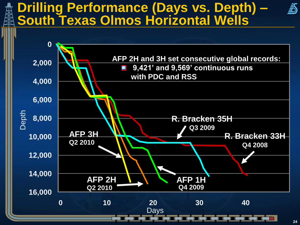
24

Drilling Performance (Days vs. Depth) –South Texas Olmos Horizontal Wells

0

2,000

4,000

6,000

8,000

10,000

12,000

14,000

16,000

0 10 20 30 40

AFP 2H Q2 2010

AFP 2H and 3H set consecutive global records:

9,421’ and 9,569’ continuous runs

with PDC and RSS

R. Bracken 33HQ4 2008

R. Bracken 35HQ3 2009

AFP 1HQ4 2009

De

pth

Days

AFP 3H Q2 2010

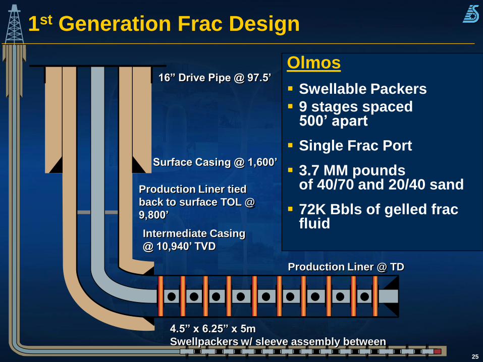
25

1st Generation Frac Design

Surface Casing @ 1,600’

Production Liner tied

back to surface TOL @

9,800’

Intermediate Casing

@ 10,940’ TVD

4.5” x 6.25” x 5m

Swellpackers w/ sleeve assembly between

Production Liner @ TD

16” Drive Pipe @ 97.5’

Olmos

Swellable Packers

9 stages spaced 500’ apart

Single Frac Port

3.7 MM pounds of 40/70 and 20/40 sand

72K Bbls of gelled fracfluid

26

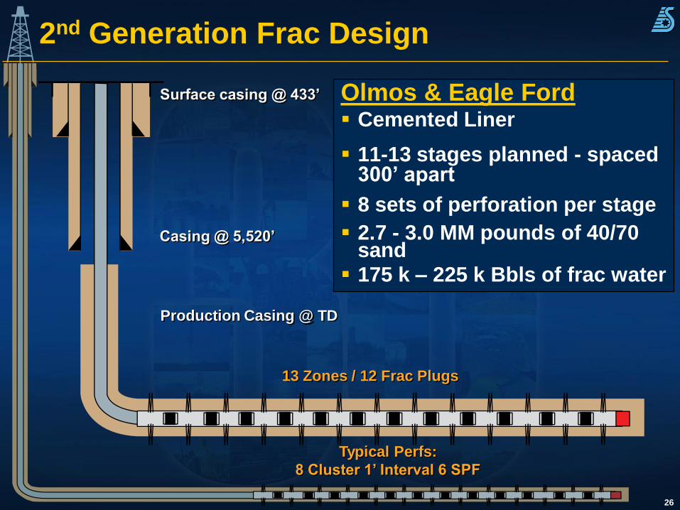
2nd Generation Frac Design

Surface casing @ 433’

Casing @ 5,520’

Production Casing @ TD

Typical Perfs:

8 Cluster 1’ Interval 6 SPF

13 Zones / 12 Frac Plugs

Olmos & Eagle Ford Cemented Liner

11-13 stages planned - spaced 300’ apart

8 sets of perforation per stage

2.7 - 3.0 MM pounds of 40/70 sand

175 k – 225 k Bbls of frac water

0

1,000

2,000

3,000

4,000

5,000

6,000

7,000

8,000

9,000

10,000

0 2,000 4,000 6,000 8,000 10,000

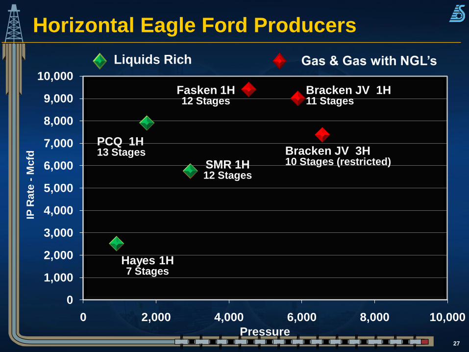
Horizontal Eagle Ford Producers

27

IP R

ate

-M

cfd

Hayes 1H7 Stages

Fasken 1H12 Stages

PCQ 1H13 Stages

Bracken JV 1H11 Stages

SMR 1H12 Stages

Pressure

Liquids Rich Gas & Gas with NGL’s

Bracken JV 3H10 Stages (restricted)

0

2,000

4,000

6,000

8,000

10,000

12,000

14,000

0 2,000 4,000 6,000 8,000 10,000

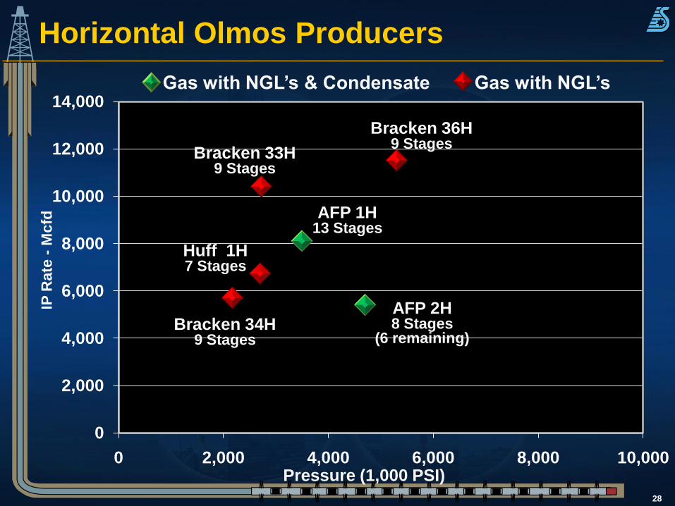
Horizontal Olmos Producers

28

Pressure (1,000 PSI)

Huff 1H7 Stages

Bracken 33H9 Stages

Bracken 34H9 Stages

Bracken 36H9 Stages

AFP 1H13 Stages

AFP 2H8 Stages

(6 remaining)

Gas with NGL’s & Condensate Gas with NGL’s

IP R

ate

-M

cfd

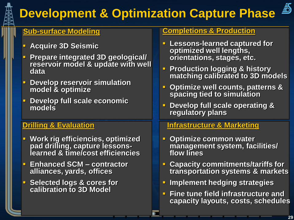
Development & Optimization Capture Phase

29

Sub-surface Modeling

Acquire 3D Seismic

Prepare integrated 3D geological/ reservoir model & update with well data

Develop reservoir simulation model & optimize

Develop full scale economic models

Drilling & Evaluation

Work rig efficiencies, optimized pad drilling, capture lessons-learned & time/cost efficiencies

Enhanced SCM – contractor alliances, yards, offices

Selected logs & cores for calibration to 3D Model

Completions & Production

Lessons-learned captured for optimized well lengths, orientations, stages, etc.

Production logging & history matching calibrated to 3D models

Optimize well counts, patterns & spacing tied to simulation

Develop full scale operating & regulatory plans

Infrastructure & Marketing

Optimize common water management system, facilities/ flow lines

Capacity commitments/tariffs for transportation systems & markets

Implement hedging strategies

Fine tune field infrastructure and capacity layouts, costs, schedules

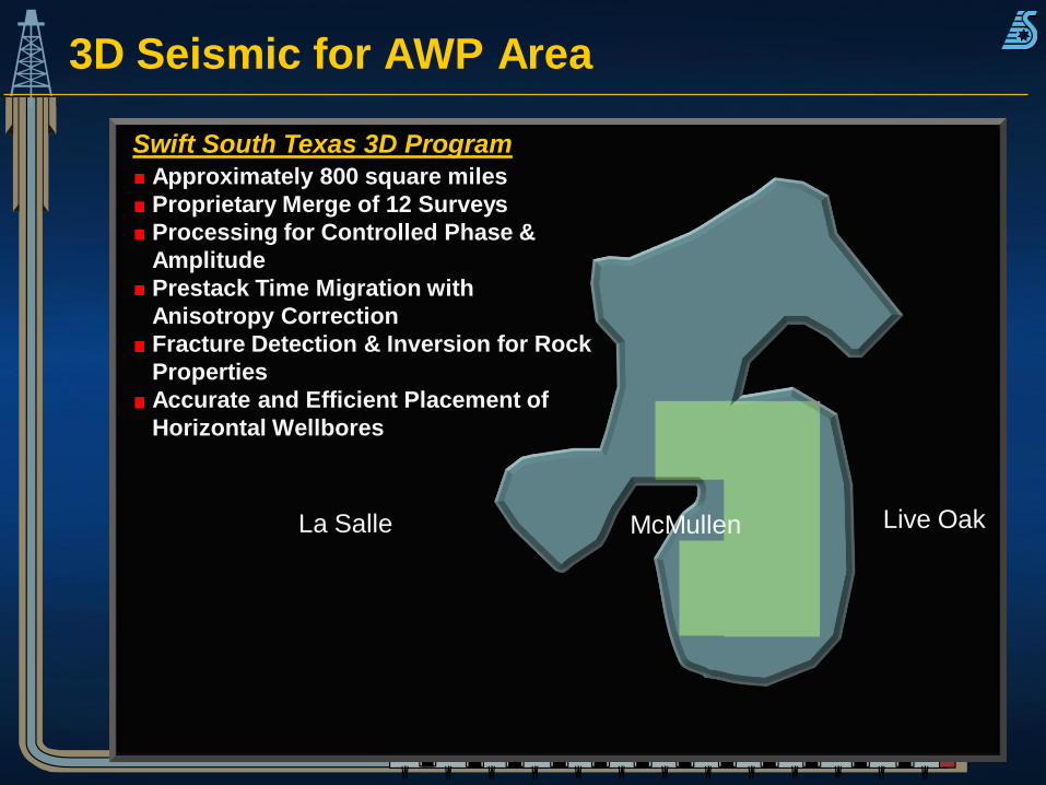
Swift South Texas 3D Program

Approximately 800 square miles

Proprietary Merge of 12 Surveys

Processing for Controlled Phase &

Amplitude

Prestack Time Migration with

Anisotropy Correction

Fracture Detection & Inversion for Rock

Properties

Accurate and Efficient Placement of

Horizontal Wellbores

3D Seismic for AWP Area

Live OakMcMullenLa Salle

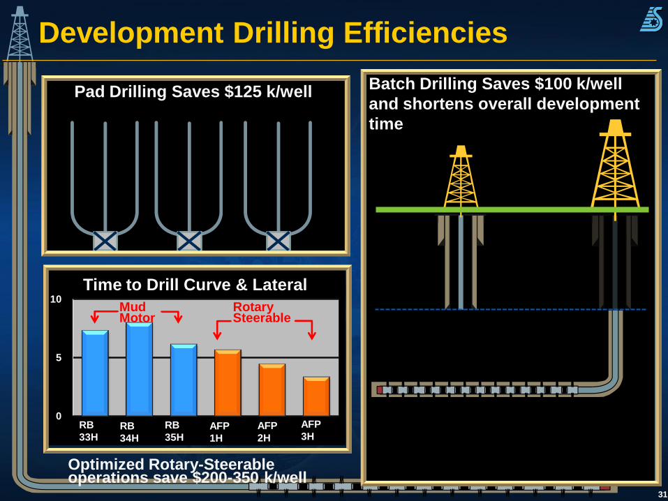
Development Drilling Efficiencies

31

Pad Drilling Saves $125 k/well

Batch Drilling Saves

$100k/well and shortens

overall development timeOptimized Rotary-Steerable operations save $200-350 k/well

Batch Drilling Saves $100 k/well

and shortens overall development

time

0

5

10 Mud Motor

Rotary Steerable

RB

33HRB

34H

AFP

1H

AFP

3HRB

35HAFP

2H

Time to Drill Curve & Lateral

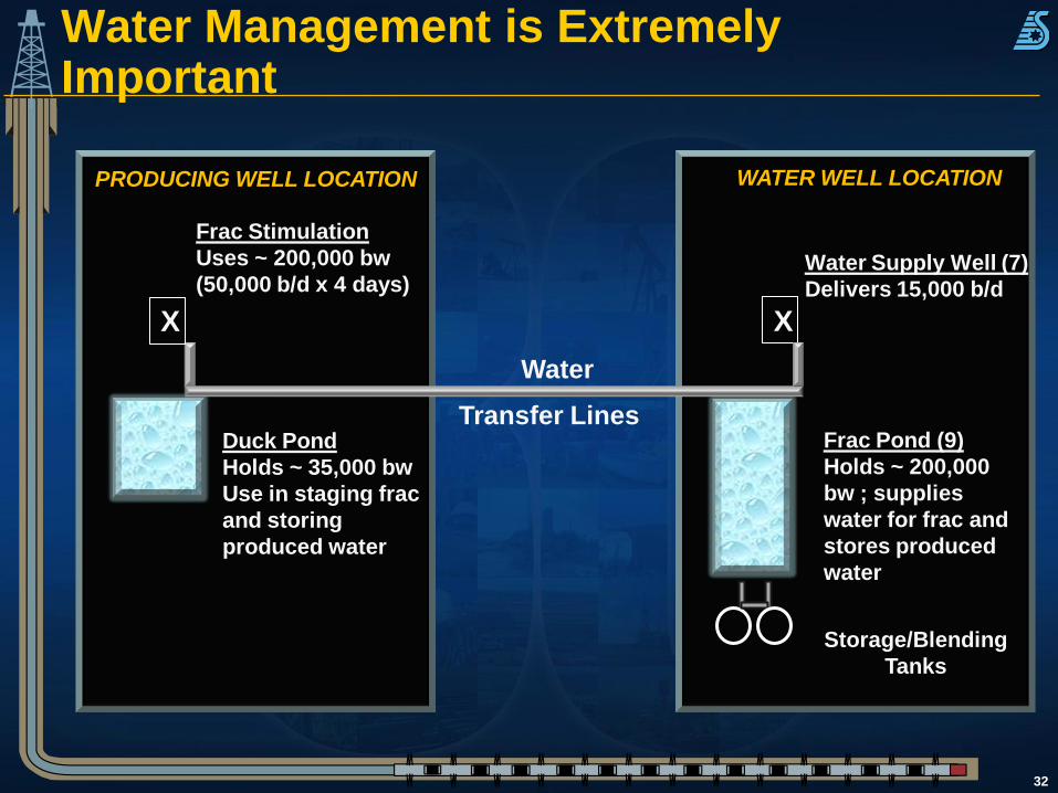
Water Management is Extremely Important

32

X

Water Supply Well (7)

Delivers 15,000 b/d

Frac Pond (9)

Holds ~ 200,000

bw ; supplies

water for frac and

stores produced

water

Water

Storage/Blending

Tanks

WATER WELL LOCATION

Frac Stimulation

Uses ~ 200,000 bw

(50,000 b/d x 4 days)

PRODUCING WELL LOCATION

Transfer Lines

X

Duck Pond

Holds ~ 35,000 bw

Use in staging frac

and storing

produced water

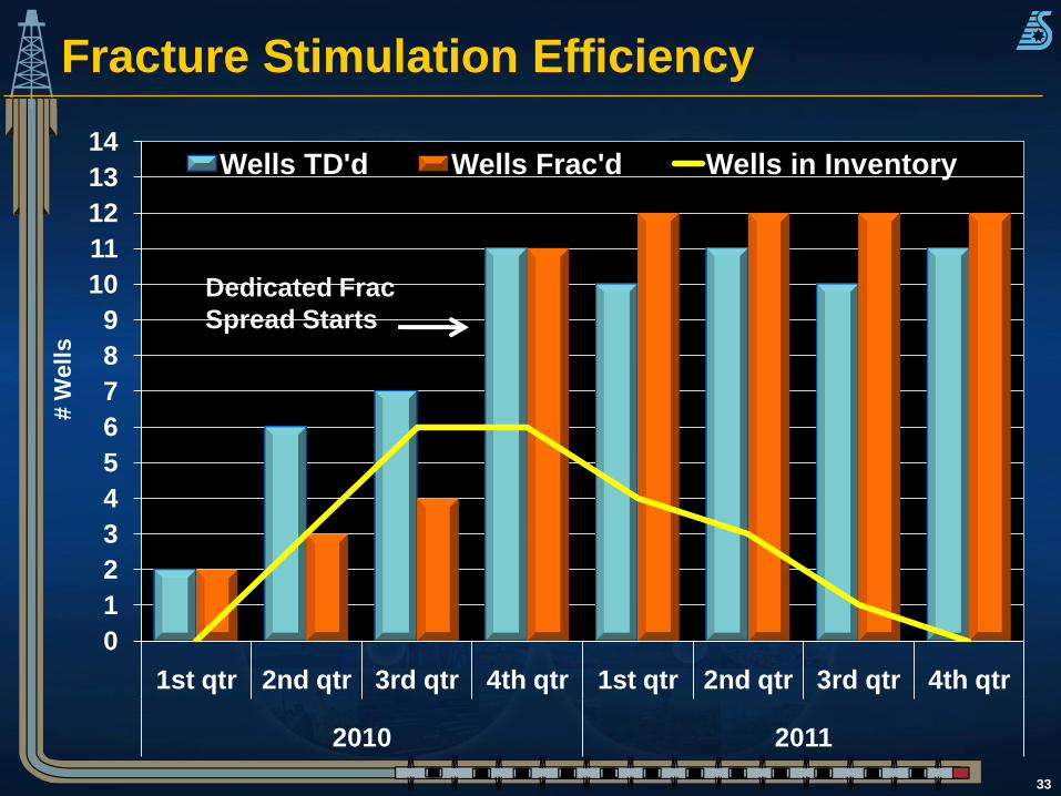
Fracture Stimulation Efficiency

33

0

1

2

3

4

5

6

7

8

9

10

11

12

13

14

1st qtr 2nd qtr 3rd qtr 4th qtr 1st qtr 2nd qtr 3rd qtr 4th qtr

2010 2011

# W

ell

s

Wells TD'd Wells Frac'd Wells in Inventory

Dedicated Frac

Spread Starts

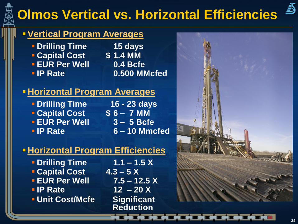
Olmos Vertical vs. Horizontal Efficiencies

Vertical Program Averages

Drilling Time 15 days Capital Cost $ 1.4 MM EUR Per Well 0.4 Bcfe IP Rate 0.500 MMcfed

Horizontal Program Averages

Drilling Time 16 - 23 days Capital Cost $ 6 – 7 MM EUR Per Well 3 – 5 Bcfe IP Rate 6 – 10 Mmcfed

Horizontal Program Efficiencies

Drilling Time 1.1 – 1.5 X Capital Cost 4.3 – 5 X EUR Per Well 7.5 – 12.5 X IP Rate 12 – 20 X

Unit Cost/Mcfe Significant Reduction

34

Eagle Ford Development Economics Dry Gas Model With Sensitivities

35

IRR

0

20

40

60

80

100

120

140

160

180

200

5.5 6 6.5 7

Well Cost $MM

$4.00 $5.00

$6.00 $7.00

0

20

40

60

80

100

120

140

160

180

200

5.5 6 6.5 7

Well Cost $MM

6 BCF ( IP = 10.8 MMcf/d )

5 BCF ( IP = 9 MMcf/d )

4 BCF ( IP = 7.2 MMcf/d )

IRR

5 BCF Case $5 Case

BFIT, After State/Local Tax & Opex

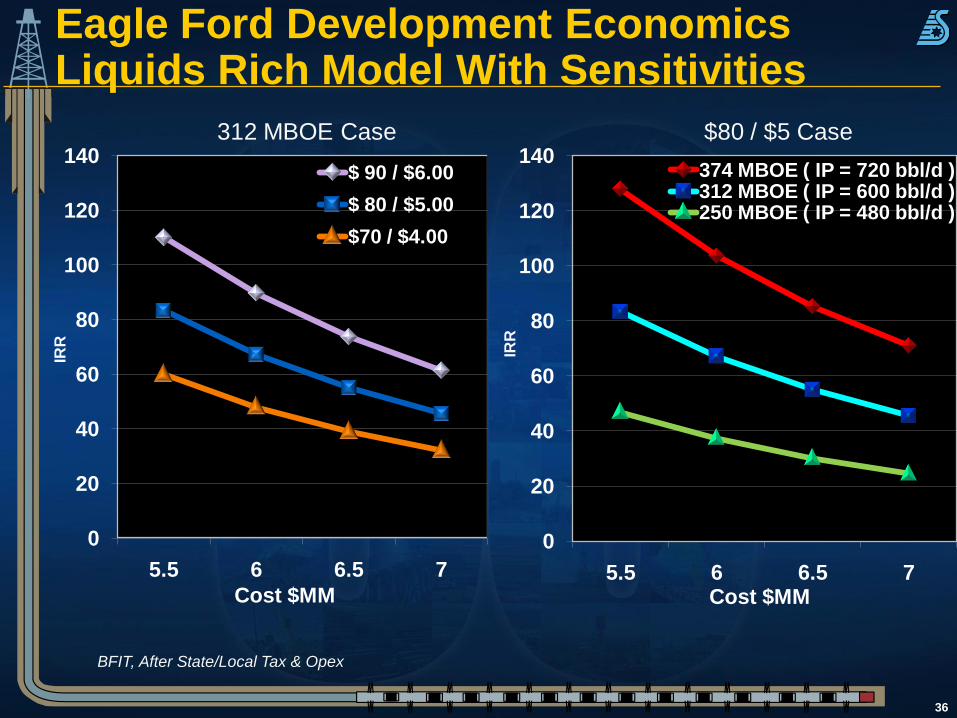
Eagle Ford Development Economics Liquids Rich Model With Sensitivities

36

IRR

0

20

40

60

80

100

120

140

5.5 6 6.5 7

Cost $MM

$ 90 / $6.00

$ 80 / $5.00

$70 / $4.00

0

20

40

60

80

100

120

140

5.5 6 6.5 7Cost $MM

374 MBOE ( IP = 720 bbl/d )312 MBOE ( IP = 600 bbl/d )250 MBOE ( IP = 480 bbl/d )

IRR

312 MBOE Case $80 / $5 Case

BFIT, After State/Local Tax & Opex

Manufacturing & Commercial Capture Phase Execute optimized Plan of Development

Squeeze operational efficiencies Supply chain management Perform benchmarking and share best practices Optimize manpower and data management

Re-calibrate reservoir performance to sub-surface and economic models

Manage transportation, sales and lease contracts

Ensure good hedging strategies

Be good stewards to all Stakeholders Ensure safe operations Protect the environment Manage the well-being of employees, investors,

contractors, landowners and community

37

30 Years of Seizing Opportunities

1979 – 2009

2010 TIPRO Central Texas Business Development Reception

October 20, 2010

“South Texas Eagle Ford and Olmos –from Unconventional to

Conventional”

“South Texas Eagle Ford and Olmos – from … Energy Presentation October 2010(2).pdf“South...

Documents

Transcript of “South Texas Eagle Ford and Olmos – from … Energy Presentation October 2010(2).pdf“South...