SOURCE IDENTIFICATION PROBLEMS FOR HYPERBOLIC...

SOURCE IDENTIFICATION PROBLEMS FOR

HYPERBOLIC DIFFERENTIAL AND DIFFERENCE

EQUATIONS

A THESIS SUBMITTED TO THE GRADUATE

SCHOOL OF APPLIED SCIENCES

OF

NEAR EAST UNIVERSITY

By

FATHI S. A. EMHARAB

In Partial Fulfillment of the Requirements for

the Degree of Doctor of Philosophy

in

Mathematics

NICOSIA, 2019

SO

UR

CE

IDE

NT

IFIC

AT

ION

PR

OB

LE

MS

FO

R H

YP

ER

BO

LIC

NE

U

FA

TH

I S. A

. EM

HA

RA

B D

IFF

ER

EN

TIA

L A

ND

DIF

FE

RE

NC

E E

QU

AT

ION

S 2

019

SOURCE IDENTIFICATION PROBLEMS FOR

HYPERBOLIC DIFFERENTIAL AND DIFFERENCE

EQUATIONS

A THESIS SUBMITTED TO THE GRADUATE

SCHOOL OF APPLIED SCIENCES

OF

NEAR EAST UNIVERSITY

By

FATHI S. A. EMHARAB

In Partial Fulfillment of the Requirements for

the Degree of Doctor of Philosophy

in

Mathematics

NICOSIA, 2019

Fathi S. A. Emharab: SOURCE IDENTIFICATION PROBLEMS FOR HYPERBOLIC

DIFFERENTIAL AND DIFFERENCE EQUATIONS

Approval of Director of Graduate School of

Applied Sciences

Prof. Dr. Nadire ÇAVUŞ

We certify this thesis is satisfactory for the award of the degree of Doctor of Philosophy of

Science in Mathematics

Examining Committee in Charge:

Prof. Dr. Evren Hinçal Committee Chairman, Department of

Mathematics, NEU

Prof. Dr. Allaberen Ashyralyev Supervisor, Department of Mathematics, NEU

Assoc. Prof. Dr. Deniz Ağırseven Department of Mathematics, Trakya University

Assoc. Prof. Dr. Okan Gerçek Department of Computer Engineering, Girne

American University

Assist. Prof. Dr. Bilgen Kaymakamzade Department of Mathematics, NEU

I hereby declare that all information in this document has been obtained and presented in

accordance with academic rules and ethical conduct. I also declare that, as required by these

rules and conduct, I have fully cited and referenced all material and results that are not

original to this work.

Name, Last name: Fathi S. A. Emharab

Signature:

Date:

iii

ACKNOWLEDGEMENT

The completion of this thesis would not be achieved without the help, backing, support,

and advice of some important individuals. There are no words that can express how

thankful and grateful I am to them.

Foremost, I would like to express my sincere gratitude to my advisor Prof. Dr. Allaberen

Ashyralyev for the continuous support of my Ph.D study and research, for his patience,

motivation, enthusiasm, and immense knowledge. His guidance helped me in all the time

of research and writing of this thesis. I could not have imagined having a better advisor and

mentor for my Ph.D study.

Besides my advisor, I would like to thank some of the great Mathematicians of our time in

persons of Prof. Dr. Charyyar Ashyralyyev for his helpful discussions and his guidance in

Matlab Implementation, Prof. Dr. Evren Hincal and Prof. Dr. Adiguzel Dosiyev for their

guidance, encouragement, and insightful comments. My appreciation also goes to staffs of

Mathematics Department Near East University, especially Dr. Hediye Sarikaya, Dr. Bilgen

Kaymakamzade, and Dr. Nuriye Sancar. Also I thank my friends Kheireddine Belakroum,

Farouk Saad, and Ayman Hamad. I thank you all for your support.

I am extremely thankful for the funding provided by the Ministry of Higher Education and

Scientific Research of Lybia.

Last but not the least, I would like to thank my family: my parents and to my wife and

brothers and sisters for supporting me spiritually throughout writing this thesis and my life

in general.

To my parents…

v

ABSTRACT

In the present study, a source identification problem with local and nonlocal conditions for

a one-dimensional hyperbolic equation is investigated. Stability estimates for the solutions

of the source identification problems are established. Furthermore, a first and second order

of accuracy difference schemes for the numerical solutions of the source identification

problems for hyperbolic equations with local and nonlocal conditions are presented.

Stability estimates for the solutions of difference schemes are established. Then, these

difference schemes are tested on examples and some numerical results are presented.

Keywords: Source identification problem; hyperbolic differential equations; difference

schemes; local and nonlocal conditions; stability; accuracy

vi

ÖZET

Bu tezde bir boyutlu bir hiperbolik denklem için yerel ve yerel olmayan koşullu bir kaynak

tanımlama problemi araştırılmıştır. Kaynak tanımlama probleminin çözümü için kararlılık

kestirimleri oluşturulmuştur. Ayrıca, hiperbolik denklemler için yerel ve yerel olmayan

koşullu kaynak tanımlama problemlerinin sayısal çözümleri için birinci ve ikinci dereceden

doğruluklu fark şemaları sunulmuştur. Fark şemalarının çözümleri için kararlılık

kestirimleri oluşturulmuştur. Daha sonra, bu fark şemaları örnekler üzerinde test edilip bazı

sayısal sonuçlar verilmiştir.

Anahtar Kelimeler: Kaynak tanımlama problemi; hiperbolik diferansiyel denklemler; fark

şemaları; yerel ve yerel olmayan koşullar; kararlılık; doğruluk

vii

TABLE OF CONTENTS

ACKNOWLEDGEMENT .............................................................................................. iii

ABSTRACT ..................................................................................................................... v

ÖZET ……………………………………………………………………….….……..….. vi

TABLE OF CONTENTS ………………………………………….………………..….. vii

LIST OF TABLES ……………………………………………………………..……….. ix

CHAPTER 1: INTRODUCTION

1.1 History …………………………………………………………………….……..…… 1

1.2 Methods of Solution of Identification Problem ……………………………….……… 5

1.3 The Aim of Thesis …………………………………………………………………… 22

CHAPTER 2: STABILITY OF THE HYPERBOLIC DIFFERENTIAL AND

DIFFERENCE EQUATION WITH LOCAL CONDITIONS

2.1 Introduction ………………………………………………………………….…..….. 23

2.2 Stability of the Differential Problem (1) …………………………………….…....… 23

2.3 Stability of the Difference Scheme ……………………………………….……....… 33

2.3.1 The first order of accuracy difference scheme ….……….…………….…….... 37

2.3.2 The second order of accuracy difference scheme ……….…………….…..….. 45

2.4 Numerical Experiments ……………………………..…………………….….…….. 55

CHAPTER 3: STABILITY OF THE HYPERBOLIC DIFFERENTIAL AND

DIFFERENCE EQUATION WITH NONLOCAL CONDITIONS

3.1 Introduction………………………………………………….……………………… 65

3.2 Stability of the Differential Problem ……………………………….…..…..….….... 65

3.3 Stability of the Difference Scheme …….……………………………….......…..….. 68

3.3.1 The first order of accuracy difference scheme ……………………........…..... 70

viii

3.3.2 The second order of accuracy difference scheme ……….……….…………. 73

3.4 Numerical Experiments ………………………………………….…………...……. 79

CHAPTER 4: CONCLUSION

Conclusion ………………………………..………………...………………….…...…... 89

REFERENCES………………………………………………………...…………….... 90

APPENDICES

Appendix 1: …………………………..……………………………………………….... 95

Appendix 2: …………………..……………….……………………………..….……... 100

Appendix 3: …………………………..……………………………..………….….…... 107

Appendix 4: …………………..……………….…………………………….….….…... 114

Appendix 5: …………………………..………………………………….….…..……... 118

ix

LIST OF TABLES

Table 1: Error analysis for difference scheme (2.69)…………………………………... 58



Table 4: Error analysis for difference scheme (3.42)……………………….……….… 82

Table 5: Error analysis for difference scheme (3.48)……………………………….…. 88

CHAPTER 1

INTRODUCTION

1.1 History

The studies of well-posed and ill-posed boundary value problems for hyperbolic and telegraph

partial differential equations are driven not only by a theoretical interest but also by the fact

of several phenomena in engineering and various fields of physics and applied sciences. In

mathematical modelling, hyperbolic and telegraph partial differential equations are used

together with boundary conditions specifying the solution on the boundary of the domain. In

some cases, classical boundary conditions cannot describe a process or phenomenon precisely.

Therefore, mathematical models of various physical, chemical, biological, or environmental

processes often involve nonclassical conditions. Such conditions are usually identified as

nonlocal boundary conditions and reflect situations when the data on the boundary of domain

cannot be measured directly, or when the data on the inside of the domain. Of great interest is

the study of absolutely stable difference schemes of a high order of accuracy for hyperbolic

partial differential equations, in which stability was established without any assumptions with

respect to the grid steps and such type of stability inequalities for the solutions of the first

order of accuracy difference scheme for the differential equations of hyperbolic type were

established for the first time ( Sobolevskii and Chebotareva, 1977).

The survey paper contains the results on the local and nonlocal well-posed problems for second

order differential and difference equations. Results on the stability of differential problems for

hyperbolic equations and of difference schemes for approximate solution of the hyperbolic

problems were presented (Ashyralyev et al., 2015).

Identification problems take an important place in applied sciences and engineering, and have

been studied by many authors (Belov, 2002; Gryazin et al., 1999; Isakov, 1998; Kabanikhin

and Krivorotko, 2015; Prilepko, Orlovsky and Vasin, 2000). The theory and applications of

source identification problems for partial differential equations have been given in various

papers ( Anikonov, 1996; Ashyralyev and Ashyralyyev, 2014; Ashyralyyev, 2014; Ashyralyyev

and Demirdag, 2012; Kozhanov, 1997; Orlovskii, 2008; Orlovskii and Piskarev, 2013).

1

In particular, Kozhanov, (1997) applied a new approach for solving elliptic equations which is

based on the transition to equations of composite type. The obtained results on solvability of

linear inverse problems for elliptic equations are based on the solvability and the properties of

solutions of boundary value problems for equations of composite type. The inverse problem

of finding the source in an abstract second-order elliptic equation on a finite interval was

studied by (Orlovskii, 2008). The additional information given is the value of the solution

at an interior point of the interval. Moreover, existence, uniqueness, and Fredholm property

theorems for the inverse problem were proved. The authors investigated an inverse problem for

an elliptic equation in a Banach space with the Bitsadze-Samarskii conditions. The suggested

approach uses the notion of a general approximation scheme, the theory of C0-semigroups of

operators and methods of functional analysis (Orlovskii and Piskarev, 2013).

The well-posedness of the unknown source identification problem for a parabolic equation

has been well investigated when the unknown function p is dependent on the space variable

(Ashyralyev, 2011; Ashyralyev, Erdogan and Demirdag, 2012; Choulli and Yamamoto, 1999;

Èidel’man, 1978; Kostin, 2013). Nevertheless, when the unknown function p is dependent

on t, the well-posedness of the source identification problem for a parabolic equation has

been investigated by (Ashyralyev and Erdogan, 2014; Borukhov and Vabishchevich, 2000;

Dehghan, 2003; Erdogan and Sazaklioglu, 2014; Ivanchov, 1995; Saitoh, Tuan and Yamamoto,

2003; Samarskii and Vabishchevich, 2008). Moreover, the well-posedness of the source

identification problem for a delay parabolic equation has also been given by (Ashyralyev and

Agirseven, 2014; Blasio and Lorenzi, 2007). The authors studied the inverse problems in

determining the coefficients of the equation for the kinetic Boltzmann equation. The Cauchy

problem and the boundary value problem for states close to equilibrium have been considered.

Theorems of the existence and uniqueness of the inverse problems were proved (Orlovskii and

Prilepko, 1987).

The solvability of the inverse problems in various formulations with various overdetermination

conditions for telegraph and hyperbolic equations were studied in many works (Anikonov,

1976; Ashyralyev and Çekiç, 2015; Kozhanov and Safiullova, 2010; Kozhanov and Safiullova,

2017; Kozhanov and Telesheva, 2017). In particular, the well-posedness of the source

2

identification problem for a telegraph equation with unknown parameter pd2v(t)

dt2 + αdv(t)

dt + Av (t) = p + f (t) ,0 ≤ t ≤ T,

v (0) = ϕ, v′ (0) = ψ, v (T) = ζ

in aHilbert space H with the self-adjoint positive-definite operator Awas proved by (Ashyralyev

and Çekiç, 2015). Here ϕ,ψ and ζ are given elements of H. They established stability estimates

for the solution of this problem. In applications, three source identification problems for

telegraph equations are developed. The authors studied the solvability of the inverse problems

on finding a solution v (x, t) and an unknown coefficient c for a telegraph equation

vtt − ∆v + cv = f (x, t) .

Theorems on the existence of the regular solutions are proved. The feature of the problems is a

presence of new overdetermination conditions for the considered class of equations (Kozhanov

and Safiullova, 2017). The authors studied solvability of the parabolic and hyperbolic inverse

problems of finding a solution together with an unknown right-hand side when the general

overdetermination condition is given. Some theorems of unique existence of regular solutions

were proved ( Kozhanov and Safiullova, 2010). The authors considered nonlinear inverse

coefficient problems for nonstationary higher-order differential equations of pseudohyperbolic

type (Kozhanov and Telesheva, 2017). More precisely, they study the problems of determining

both the solution of the corresponding equation, an unknown coefficient at the solution or at

the time derivative of the solution in the equation. A distinctive feature of these problems is

the fact that the unknown coefficient is a function of time only. Integral overdetermination is

used as an additional condition. The existence theorems of regular solutions (those solutions

that have all generalized derivatives in the sense of S. L. Sobolev) were proved. The technique

of the proof relies on the transition from the original inverse problem to a new direct problem

for an auxiliary integral-differential equation, and then on the proof of solvability of the latter

and construction of some solution of the original inverse problem from a solution of the

auxiliary problem. A theorem on the uniqueness for solutions to an inverse problem for the

wave equation has been proved (Anikonov, 1976). Finally, some new representations were

given for the solutions and coefficients of the equations of mathematical physics (Anikonov,

3

1995; Anikonov, 1996; Anikonov and Neshchadim, 2011; Anikonov and Neshchadim, 2012

a, 2012b). Their main direction of study was to search for reciprocal formulas connecting

solutions and coefficients, and involving arbitrary functions as well as functions satisfying

some differential relations. They gave such formulas for evolution equations of first and

second order in time, in particular for parabolic and hyperbolic equations in the linear and

nonlinear cases.

In this thesis, we consider the time-dependent source identification problem for a one-

dimensional hyperbolic equation with local conditions

∂2u (t, x)∂t2 −

∂

∂x

(a (x)

∂u (t, x)∂x

)= p (t) q (x) + f (t, x) ,

x ∈ (0, l) , t ∈ (0,T) ,

u (0, x) = ϕ (x) ,ut (0, x) = ψ (x) , x ∈ [0, l] ,

u (t,0) = u (t, l) = 0,∫ l0 u (t, x) dx = ζ (t) , t ∈ [0,T]

(1.1)

and with nonlocal conditions

∂2u (t, x)∂t2 −

∂

∂x

(a (x)

∂u (t, x)∂x

)+ δu (t, x) = p (t) q (x) + f (t, x) ,

x ∈ (0, l) , t ∈ (0,T) ,

u (0, x) = ϕ (x) ,ut (0, x) = ψ (x) , x ∈ [0, l] ,

u (t,0) = u (t, l) ,ux (t,0) = ux (t, l) ,∫ l0 u (t, x) dx = ζ (t) , t ∈ [0,T] ,

(1.2)

where u (t, x) and p (t) are unknown functions, a (x) ≥ a > 0, δ ≥ 0, f (t, x) , ζ (t) , ϕ (x) and

ψ (x) are sufficiently smooth functions, and q (x) is a sufficiently smooth function assuming∫ l0 q (x) dx , 0, and q (0) = q (l) = 0 for (1.1), q (0) = q (l) , q′ (0) = q′ (l) for (1.2). At the

same time, we note that the inverse problems (1.1) and (1.2) for the hyperbolic equation were

not studied before. Basic results of this thesis have been published by the following papers

(Ashyralyev and Emharab, 2017; Ashyralyev and Emharab, 2018a, 2018b, 2018c, 2018d).

Some results of this work were presented in Mini-symposium "Inverse Ill-posed Problems

and its applications" of VI congress of Turkic World Mathematical Society (TWMS 2017),

and 2nd International Conference of Mathematical Sciences, 2018.

4

1.2 Methods of Solution of Source Identification Problem

It is known that local and nonlocal boundary value problems for second order partial differential

equations can be solved analytically by Fourier series, Laplace transform and Fourier transform

methods. Now, let us illustrate these three different analytical methods by examples. Let us

see how to apply the classic methods, namely, Fourier series, Fourier transform and Laplace

transform for obtaining the solution of source identification problem for hyperbolic equations

on some examples.

Example 1.2.1 Obtain the Fourier series solution of the following source identification

problem

∂2u (t, x)∂t2 −

∂2u (t, x)∂x2 = p (t) sin x + e−t sin x,

0 < x < π,0 < t < 1,

u (0, x) = sin x,ut (0, x) = − sin x,0 ≤ x ≤ π,

u (t, π) = u (t,0) = 0,∫ π

0 u (t, x) dx = 2e−t,0 ≤ t ≤ 1,

(1.3)

for a one dimensional hyperbolic equation.

Solution. In order to solve the problem, we consider the Sturm-Liouville problem

uxx − λu (x) = 0,0 < x < π, u (0) = u (x) = 0,

generated by the space operator of problem (1.3). It is easy to see that the solution of this

Sturm-Liouville problem is

λk = −k2,uk(x) = sin k x, k = 1,2, ....

Therefore, we will seek solution u(t, x) using by the Fourier series

u (t, x) =∞∑

k=1Ak (t) sin k x. (1.4)

Here Ak (t) , k = 1,2... are unknown functions. Putting (1.4) into the equation (1.3) and using

given initial and boundary conditions, we obtain

∞∑k=1

A′′k (t) sin k x +∞∑

k=1k2 Ak (t) sin k x = p (t) sin x + e−t sin x,

5

u (0, x) =∞∑

k=0Ak (0) sin k x = sin x,

ut (0, x) =∞∑

k=0A′k (0) sin k x = − sin x,

∫ π

0u (t, x) dx =

∫ π

0

∞∑k=1

Ak (t) sin k xdx = −∞∑

k=1

Ak (t) cos k xk

π0

=

∞∑k=1

Ak (t)

[1 + (−1)k+1

k

]= 2e−t .

Equating the coefficients of sin k x, k = 1,2... to zero, we get

A′′k (t) + k2 Ak (t) = 0, k , 1, A′′1 (t) + A1 (t) = p (t) + e−t,0 < t < 1,

Ak (0) = 0, A′k (0) = 0, k , 1, A1 (0) = 1, A′1 (0) = −1,∞∑

k=1Ak (t)

[1 + (−1)k+1

k

]= 2e−t,0 < t < 1. (1.5)

First, we will obtain Ak (t) for k , 1. It is easy to see that Ak (t) is the solution of the

following Cauchy problem

A′′k (t) + k2 Ak (t) = 0, 0 < t < 1, Ak (0) = 0, A′k (0) = 0,

for the second order differential equations. Its solution is Ak (t) ≡ 0, k , 1. From that and

formula (1.5), we get

−2A1 (t) = −2e−t .

Therefore,

A1 (t) = e−t . (1.6)

Second,we will obtain p (t). It is clear that A1 (t) is solution of the following Cauchy problem

A′′1 (t) + A1 (t) = p (t) + 2e−t, 0 < t < 1, A1 (0) = 1, A′1 (0) = −1, (1.7)

for the second order differential equations. Applying (1.6) and (1.7),we obtain

p (t) = e−t .

6

Then, (1.4) becomes u (t, x) = A1 (t) sin x = e−t sin x. Therefore, the exact solution of problem

(1.3) is (u (t, x) , p (t)) =(e−t sin x, e−t ) .

Note that using similar procedure one can obtain the solution of the following source

identification problem

∂2u(t, x)∂t2 −

n∑r=1

αr∂2u(t, x)∂x2

r= p(t)q(x) + f (t, x),

x = (x1, ..., xn) ∈ Ω, 0 < t < T,

u(0, x) = ϕ(x), ut(0, x) = ψ (x) , x ∈ Ω,

u(t, x) = 0, 0 ≤ t ≤ T, x ∈ S,∫· · ·

∫x∈Ω

u (t, x) dx1...dxn = ξ(t),0 ≤ t ≤ T,

(1.8)

for the multidimensional hyperbolic partial differential equation. Assume that αr > α > 0

and f (t, x) ,q (x) , (t ∈ (0,T) , x ∈ Ω), ϕ(x),ψ (x) ,(x ∈ Ω

), ξ(t), (t ∈ [0,T]) are given smooth

functions. Here and in future Ω is the unit open cube in the n−dimensional Euclidean space

Rn (0 < xk < 1,1 ≤ k ≤ n) with the boundary S and Ω = Ω ∪ S.

Example 1.2.2 Obtain the Fourier series solution of the following source identification

problem

∂2u (t, x)∂t2 +

∂u (t, x)∂x2 = p (t) (1 + sin 2x) + 4e−t sin 2x,

0 < t < 1,0 < x < π,

u (0, x) = 1 + sin 2x,ut (0, x) = − (1 + sin 2x) , 0 ≤ x ≤ π,

u (t,0) = u (t, π) ,ux (t,0) = ux (t, π) , 0 ≤ t ≤ 1,∫ π

0 u (t, x) dx = e−tπ, 0 ≤ t ≤ 1,

(1.9)


Solution. In order to solve this problem, we consider the Sturm-Liouville problem

uxx − λu (x) = 0,0 < x < π, u (0) = u (x) , ux (0) = ux (π)

7



λk = 4k2,uk (x) = cos 2k x, k = 0,1,2, ..., uk (x) = sin 2k x, k = 1,2, ....

Therefore, we will seek solution u(t, x) using by the Fourier series

u (t, x) =∞∑

k=0Ak (t) cos 2k x +

∞∑k=1

Bk (t) sin 2k x, (1.10)

where Ak (t) , k = 0,1,2, ... and Bk (t) , k = 1,2, ... are unknown functions, Putting (1.10) into

(1.9) and using given initial and boundary conditions, we get

∞∑k=0

A′′k (t) cos 2k x +∞∑

k=1B′′k (t) sin 2k x +

∞∑k=0

4k2 Ak (t) cos k x

+

∞∑k=1

4k2Bk (t) sin 2k x = p (t) (sin 2x + 1) + 4e−t sin 2x,

u (0, x) =∞∑

k=0Ak (0) cos 2k x +

∞∑k=1

Bk (0) sin 2k x = sin 2x + 1,

ut (0, x) =∞∑

k=0A′k (0) cos 2k x +

∞∑k=1

B′k (0) sin 2k x = − sin 2x − 1,

∫ π

0u (t, x) dx =

∫ π

0

[∞∑

k=0Ak (t) cos 2k x +

∞∑k=1

Bk (t) sin 2k x

]dx

= A0 (t) π +∞∑

k=1

Ak (t) sin 2k x2k

]π0

−

∞∑k=1

Bk (t) cos 2k x2k

]π0

= A0 (t) π = e−tπ.

From that it follows that A0 (t) = e−t . Equating the coefficients of cos k x, k = 0,1,2, ... and

sin k x, k = 1,2, ... to zero, we getA′′k (t) + 4k2 Ak (t) = 0, 0 < t < 1,

Ak (0) = 0, A′k (0) = 0, k , 0,(1.11)

A′′0 (t) = p (t) , 0 < t < 1,

A0 (0) = 1, A′0 (0) = −1,(1.12)

8

B′′k (t) + 4k2Bk (t) = 0, 0 < t < 1,

Bk (0) = 0,B′k (0) = 0,(1.13)

B′′1 (t) + 4B1 (t) = p (t) + 4e−t, 0 < t < 1,

B1 (0) = 1,B′1 (0) = −1.(1.14)

First, we obtain p(t). Applying problem (1.12) and A0(t) = e−t,we get

p (t) = e−t .

Second, we obtain Ak(t), k , 0. It is clear that for k , 0, Ak(t) is the solution of the initial

value problems (1.11) and (1.12). The auxiliary equation is

m2 + 4k2 = 0.

We have two roots

m1 = 2ik,m2 = −2ik

Therefore,

Ak (t) = c1 cos 2kt + c2 sin 2kt.

Applying initial conditions Ak (0) = A′k (0) = 0,we get

Ak (0) = c1 = 0,

A′k (0) = 2kc2 = 0.

Then c1 = c2 = 0 and Ak (t) = 0, k , 0. Third, we obtain Bk(t). It is clear that for k , 1,Bk(t)

is the solution of the initial value problem (1.13). The auxiliary equation is

m2 + 4k2 = 0.

We have two roots

m1 = 2ik,m2 = −2ik .

Therefore,

Bk (t) = c1 cos 2kt + c2 sin 2kt.

9

Applying initial conditions Bk (0) = B′k (0) = 0,we get

Bk (0) = c1 = 0,

B′k (0) = 2kc2 = 0.

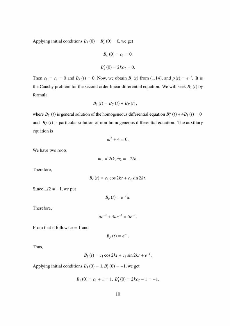
Then c1 = c2 = 0 and Bk (t) = 0. Now, we obtain B1 (t) from (1.14), and p (t) = e−t . It is

the Cauchy problem for the second order linear differential equation. We will seek B1 (t) by

formula

B1 (t) = BC (t) + BP (t) ,

where BC (t) is general solution of the homogeneous differential equation B′′1 (t)+ 4B1 (t) = 0

and BP (t) is particular solution of non-homogeneous differential equation. The auxiliary

equation is

m2 + 4 = 0.

We have two roots

m1 = 2ik,m2 = −2ik .

Therefore,

Bc (t) = c1 cos 2kt + c2 sin 2kt.

Since ±i2 , −1,we put

Bp (t) = e−ta.

Therefore,

ae−t + 4ae−t = 5e−t .

From that it follows a = 1 and

Bp (t) = e−t .

Thus,

B1 (t) = c1 cos 2kt + c2 sin 2kt + e−t .

Applying initial conditions B1 (0) = 1,B′1 (0) = −1,we get

B1 (0) = c1 + 1 = 1, B′1 (0) = 2kc2 − 1 = −1.

10

From that it follows

B1 (t) = e−t .

Therefore,

u (t, x) = e−t (sin 2x + 1) .

So, the exact solution of problem (1.9) is

(u (t, x) , p (t)) =(e−t (sin 2x + 1) , e−t ) .



∂2u(t, x)∂t2 −

n∑r=1

αr∂2u(t, x)∂x2

r= p (t) q (x) + f (t, x),

x = (x1, ..., xn) ∈ Ω, 0 < t < T,

u(0, x) = ϕ(x),ut(0, x) = ψ (x) , x ∈ Ω,

u(t, x)|S1 = u(t, x)|S2 ,∂u(t, x)∂m

S1

=∂u(t, x)∂m

S2

,∫· · ·

∫x∈Ω

u (t, x) dx1...dxn = ξ(t),0 ≤ t ≤ T,

(1.15)

for the multidimensional hyperbolic partial differential equation. Assume that αr > α > 0 and

f (t, x) ,q (x) , (t ∈ (0,T) , x ∈ Ω) ,ψ (x) , ξ(t),(t ∈ [0,T] , x ∈ Ω

)are given smooth functions.

Here S = S1 ∪ S2,S1 ∩ S2 = ∅, and m is the normal vector to S1 and S2.

However Fourier series method described in solving (1.8) and (1.15) can be used only in the

case when (1.8) and (1.15) have constant coefficients.

Second, we consider the Laplace transform method for solution of the source identification

problem for hyperbolic differential equation.

Example 1.2.3 Obtain the Laplace transform solution of the following source identifica-

11

tion problem

∂2u (t, x)∂t2 −

∂2u (t, x)∂x2 + 2u (t, x) = p (t) e−x + e−t−x,

0 < x < ∞,0 < t < 1,

u (0, x) = e−x,ut (0, x) = −e−x,0 ≤ x < ∞,

u (t,0) = e−t,ux (t,0) = −e−t,0 ≤ t ≤ 1,∫ ∞0 u (t, x) dx = e−t,0 ≤ t ≤ 1,0 ≤ x < ∞,

(1.16)


Solution. We will denote

L u(t, x) = u(t, s).

Using formula

L e−x =1

s + 1(1.17)

and taking the Laplace transform of both sides of the differential equation and conditions

u(t,0) = e−t,ux(t,0) = −e−t , we can write

L utt (t, x) − L uxx (t, x) + 2L u (t, x) =[p (t) + e−t ] L e−x ,

L u (0, x) = L e−x ,L ut (0, x) = −L e−x

or utt (t, s) − s2u (t, s) + su (t,0) + ux (t,0) + 2u (t, s) = p (t) 1

s+1 + e−t 1s+1,

u(0, s) =1

s + 1,ut(0, s) = −

1s + 1

.

Therefore, we get the following problemutt (t, s) +

(2 − s2) u (t, s) + se−t − e−t = p (t) 1

s+1 + e−t 1s+1,

u(0, s) =1

s + 1,ut(0, s) = −

1s + 1

.

Applying the condition ∫ ∞

0u (t, x) dx = e−t,0 ≤ t ≤ 1,

and the definition of the Laplace transform, we get

u (t,0) = e−t,0 ≤ t ≤ 1, (1.18)

12

It is clear that u(t, s) is solution of the following source identification problemutt (t, s) +

(2 − s2) u (t, s) = p (t) 1

s+1 +2−s2

s+1 e−t,

u (0, s) = 1s+1,ut (0, s) = 1

s+1 .(1.19)

Applying the D’Alembert’s formula, we obtain

u (t, s) =1

s + 1cos

√2 − s2t −

1s + 1

1√

2 − s2sin

√2 − s2t (1.20)

+1

√2 − s2

∫ t

0sin

√2 − s2 (t − y)

p (y)

1s + 1

+2 − s2

s + 1e−y

dy.

Now, we will apply the condition (1.18) with (1.20), we get

e−t = cos√

2t −1√

2sin√

2t +1√

2

∫ t

0sin√

2 (t − y) p (y) + 2e−y dy. (1.21)

Taking the first and second order derivatives, we get

−e−t = −√

2 sin√

2t − cos√

2t +∫ t

0cos√

2 (t − y) p (y) + 2e−y dy,

e−t = −2 cos√

2t +√

2 sin√

2t

−√

2∫ t

0sin√

2 (t − y) p (y) + 2e−y dy + p (t) + 2e−t . (1.22)

Applying (1.21) and (1.22), we get

e−t = −2 cos√

2t +√

2 sin√

2t + p (t) + 2e−t

−√

2√

2e−t − cos

√2t +

1√

2sin√

2t.


p (t) = e−t . (1.23)

Finally, applying (1.20) and (1.23), we get

u (t, s) =1

s + 1cos

√2 − s2t −

1s + 1

1√

2 − s2sin

√2 − s2t

+1

√2 − s2

∫ t

0sin

√2 − s2 (t − y)

e−y

(3 − s2

s + 1

)dy.

13

Applying the formula∫ t

0sin

√2 − s2 (t − y) e−ydy =

sin√

2 − s2t + e−t√

2 − s2 −√

2 − s2 cos√

2 − s2t3 − s2 ,

we get

u (t, s) =1

s + 1cos

√2 − s2t −

1s + 1

1√

2 − s2sin

√2 − s2t

+1

√2 − s2

3 − s2

s + 1

[sin√

2 − s2t + e−t√

2 − s2 −√

2 − s2 cos√

2 − s2t3 − s2

]=

1s + 1

cos√

2 − s2t −1

s + 11

√2 − s2

sin√

2 − s2t

+1

√2 − s2

1s + 1

sin√

2 − s2t +e−t

s + 1−

1s + 1

cos√

2 − s2t = e−t 1s + 1

. (1.24)

From that it follows that

u (t, x) = e−tL−1

1s + 1

= e−t−x .

Therefore, the exact solution of problem (1.16) is

(u (t, x) , p (t)) =(e−t−x, e−t ) .

Example 1.2.4 Obtain the Laplace transform solution of the following source identification

problem

∂2u (t, x)∂t2 +

∂u (t, x)∂t

= p (t) (1 + sin 2x) + 4e−t sin 2x,

t > 0,0 < x < π,

u (0, x) = 1 + sin 2x, ut (0, x) = − (1 + sin 2x) , 0 ≤ x ≤ π,

u (t,0) = u (t, π) ,ux (t,0) = ux (t, π) , t ≥ 0,∫ π

0 u (t, x) dx = e−tπ, 0 ≤ t ≤ 1,

(1.25)


Solution. We will denote

L u(t, x) = u(s, x).

14

Using formula

Le−t = 1

s + 1and taking the Laplace transform of both sides of the differential equation and conditions

u(0, x) = 1 + sin 2x,ut(0, x) = −(1 + sin 2x), we can writes2u (s, x) − u (s,0) − ux (t,0) + uxx (s, x)

= p (s) (1 + sin 2x) + 41+s sin 2x,

u (s,0) = u (s, π) ,ux (s,0) = ux (s, π) , 0 ≤ t ≤ 1.

Therefore, we get the following problem

s2u (s, x) − s (1 + sin 2x) + (1 + sin 2x) − uxx (s, x)

= p (s) (1 + sin 2x) + 41+s sin 2x,

u (t,0) = u (t, π) ,ux (t,0) = ux (t, π) ,∫ π

0 u (s, x) dx = π1+s , 0 ≤ t ≤ 1.

(1.26)

In order to solve this problem, we consider the Sturm-Liouville problem

uxx − λu (x) = 0,0 < x < π, u (0) = u (x) , ux (0) = ux (π)



λk = 4k2,uk (x) = cos 2k x, k = 0,1,2, ..., uk (x) = sin 2k x, k = 1,2, ....

Then, we will obtain the Fourier series solution of problem (1.26) by formula

u (s, x) =∞∑

k=0Ak (s) cos 2k x +

∞∑k=1

Bk (s) sin 2k x, (1.27)

where Ak (t) , k = 0,1,2, ... and Bk (t) , k = 1,2, ...are unknown functions, Putting (1.27) into

(1.26) and using given initial and boundary conditions, we get

s2∞∑

k=0Ak (s) cos 2k x − s (1 + sin 2x) + (1 + sin 2x)

+s2∞∑

k=1Bk (s) sin 2k x +

∞∑k=0

4k2 Ak (s) cos k x

15

+

∞∑k=1

4k2Bk (s) sin 2k x = p (s) (1 + sin 2x) +4

1 + ssin 2x,

u (0, x) =∞∑

k=0Ak (0) cos 2k x +

∞∑k=1

Bk (0) sin 2k x = 1 + sin 2x,

ut (0, x) =∞∑

k=0A′k (0) cos 2k x +

∞∑k=1

B′k (0) sin 2k x = −1 − sin 2x,

∫ π

0u (s, x) dx =

∫ π

0

[∞∑

k=0Ak (s) cos 2k x +

∞∑k=1

Bk (s) sin 2k x

]dx

= A0 (s) π +∞∑

k=1

Ak (s) sin 2k x2k

]π0

−

∞∑k=1

Bk (s) cos 2k x2k

]π0

= A0 (s) π =π

1 + s.

From that it follows A0 (s) = 11+s . Equating the coefficients of cos k x, k = 0,1,2, ... and

sin k x, k = 1,2, ... to zero, we gets2 Ak (s) + 4k2 Ak (s) = 0, k , 0,

Ak (0) = 0, A′k (0) = 0,and Ak (s) = 0, k , 0,(1.28)

s2 A0 (s) − s + 1 = p (s) ,

A0 (0) = 1, A′0 (0) = −1,(1.29)

s2Bk (s) + 4k2Bk (s) = 0,

Bk (0) = 0,B′k (0) = 0,and Bk (s) = 0, k , 0,(1.30)

s2B1 (s) + 4B1 (s) − s + 1 = p (s) + 4

s+1,

B1 (0) = 1, B′1 (0) = 1.(1.31)

First, we obtain p(s). Applying problem (1.29) and A0(t) = 11+s ,we get

p (s) =1

1 + s.

Second, we obtain B1 (t) from (1.31) and p (s) = 11+s ,where(

s2 + 4)

B1 (s) − s + 1 =1

1 + s+

4s + 1

,

Thus,

B1 (s) =1

1 + s.

16

Then, (1.27) becomes

u (s, x) =1

1 + s+

11 + s

sin 2x,


u (t, x) = L−1

11 + s

+1

1 + ssin 2x

= e−t (1 + sin 2x) .

Therefore, the exact solution of problem (1.25) is

u (t, x) , p (t) =e−t (1 + sin 2x) , e−t .



∂2u(t, x)∂t2 −

n∑r=1

ar∂2u(t, x)∂x2

r= p(t)q(x) + f (t, x),

x = (x1, ..., xn) ∈ Ω+, 0 < t < T,

u(0, x) = ϕ(x),ut(0, x) = ψ (x) x ∈ Ω+,

u(t, x) = α (t, x) , uxr (t, x) = β (t, x) ,

1 ≤ r ≤ n,0 ≤ t ≤ T, x ∈ S+,∫ x10 ...

∫ xn0 u (t, x) dx1...dxn = ξ(t),0 ≤ t ≤ T,

(1.32)

for the multidimensional hyperbolic partial differential equation. Assume that

ar > a > 0 and f (t, x) ,(t ∈ (0,T) , x ∈ Ω

+), ξ(t), (t ∈ [0,T]), ϕ(x),ψ (x)

(x ∈ Ω

+),

α (t, x) , β (t, x) (t ∈ [0,T] , x ∈ S+) are given smooth functions. Here and in future Ω+ is

the open cube in the n-dimensional Euclidean space Rn (0 < xk < ∞,1 ≤ k ≤ n) with the

boundary S+ and Ω+= Ω+ ∪ S+.

However Laplace transform method described in solving (1.32) can be used only in the case

when (1.32) has constant or polynomial coefficients.

Third, we consider Fourier transform method for solution of the source identification problem

for hyperbolic differential equations.

17

Example 1.2.5 Obtain the Fourier transform solution of the following source identifica-

tion problem

∂2u (t, x)∂t2 −

∂2u (t, x)∂x2 = p (t) e−x2

−(4x2 + 2

)e−t−x2

,

−∞ < x < ∞,0 < t < 1,

u (0, x) = e−x2,ut (0, x) = −e−x2

, x ∈ (−∞,∞) ,∫ ∞−∞

u (t, x) dx = e−t√π, t ≥ 0,

(1.33)


Solution. Let us denote

F u (t, x) = u (t, µ) .

Taking the Fourier transform of both sides of the differential equation and initial conditions

(1.33), we can obtainutt (t, µ) + µ2u (t, µ) = p (t) F

e−x2

−e−tF

d2

dx2

(e−x2

),0 < t < 1,

u (0, µ) = Fe−x2

,ut (0, µ) = −F

e−x2

.

(1.34)

Then, we obtain u (t, µ) as the solution of the following Cauchy problemutt (t, µ) + µ2u (t, µ) =

(p (t) + µ2e−t ) F

e−x2,0 < t < 1,

u (0, µ) = Fe−x2

,ut (0, µ) = −F

e−x2

.

(1.35)

Using the D’Alembert’s formula, we obtain

u (t, µ) =eiµt + e−iµt

2F

e−x2

−

eiµt − e−iµt

2iµF

e−x2

+

∫ t

0

eiµ(t−s) − e−iµ(t−s)

2iµ

[(p (s) + µ2e−s

)F

e−x2

]ds

or

u (t, µ) =eiµt + e−iµt

2F

e−x2

−

12

∫ t

−teiµydy

(F

e−x2

)+

12

∫ t

0

∫ t−s

−(t−s)eiµydy

[(p (s) + µ2e−s

)F

e−x2

]ds.

18

Using the formula F f (x ± t) = e±iµtF f (x) ,we obtain

u (t, µ) =12

[F

e−(x+t)2

+ F

e−(x−t)2

]−

12

∫ t

−tF

e−(x+y)

2

dy

+12

∫ t

0

∫ t−s

−(t−s)p (s) F

e−(x+y)

2

dyds +12

∫ t

0

∫ t−s

−(t−s)e−sµ2F

e−(x+y)

2

dyds.

Since µ2Fe−x2

= −F

d2

dx2

(e−x2

),we have that

u (t, µ) =12

[F

e−(x+t)2

+ F

e−(x−t)2

]−

12

∫ t

−tF

e−(x+y)

2

dy

+12

∫ t

0p (s)

∫ t−s

−(t−s)F

e−(x+y)

2

dyds −12

∫ t

0e−s

∫ t−s

−(t−s)F

∂2

∂y2

(e−(x+y)

2)

dyds.

Taking the inverse Fourier transform, we obtain

u (t, x) = F −1 u (t, µ) =12

[e−(x+t)2 + e−(x−t)2

]−

12

∫ t

−te−(x+y)

2dy

+12

∫ t

0p (s)

∫ t−s

−(t−s)e−(x+y)

2dyds −

12

∫ t

0e−s

∫ t−s

−(t−s)

∂2

∂y2

(e−(x+y)

2)

dyds.

Now, applying condition∫ ∞−∞

u (t, x) dx = e−t√π,we obtain

e−t√π =12

[∫ ∞

−∞

e−(x+t)2 dx +∫ ∞

−∞

e−(x−t)2 dx]−

12

∫ t

−t

∫ ∞

−∞

e−(x+y)2dxdy

+12

∫ t

0p (s)

∫ t−s

−(t−s)

∫ ∞

−∞

e−(x+y)2dxdyds −

12

∫ t

0e−s

∫ t−s

−(t−s)

∫ ∞

−∞

∂2

∂y2

(e−(x+y)

2)

dxdyds.

Since∫ ∞−∞

e−x2dx =

√π,we can write

e−t√π =√π −√πt +√π

∫ t

0(t − s) p (s) ds −

12

∫ t

0e−s

∫ t−s

−(t−s)

∫ ∞

−∞

∂2

∂y2

(e−(x+y)

2)

dxdyds.

Since∂2

∂y2

(e−(x+y)

2)= 4 (x + y)2 e−(x+y)

2− 2e−(x+y)

2,

we have that

∫ ∞

−∞

∂2

∂y2

(e−(x+y)

2)

dx = 4∫ ∞

−∞

(x + y)2 e−(x+y)2dx − 2

∫ ∞

−∞

e−(x+y)2dx

19

= 4∫ ∞

−∞

p2e−p2dp − 2

∫ ∞

−∞

e−p2dp = −2

∫ ∞

−∞

pd(e−p2

)− 2√π

= 2∫ ∞

−∞

e−p2dp − 2

√π = 2

√π − 2

√π = 0.

Therefore,

e−t = 1 − t +∫ t

0(t − s) p (s) ds.


−e−t = −1 +∫ t

0p (s) ds.

Taking the derivative, we obtain

e−t = p (t) .

Putting p (t) into the given differential equation (1.35), we obtain the following Cauchy

problem utt (t, µ) + µ2u (t, µ) = e−t (

1 + µ2) F e−x2

,0 < t < 1,

u (0, µ) = Fe−x2

,ut (0, µ) = −F

e−x2

.

We will seek the general solution u (t, µ) of this equation by the following formula

u (t, µ) = uc (t, µ) + up (t, µ) ,

where uc (t, µ) is the solution of homogeneous equation

utt (t, µ) + µ2u (t, µ) = 0,0 < t < 1

and up (t, µ) is the particular solution of nonhomogeneous equation

utt (t, µ) + µ2u (t, µ) = e−t(1 + µ2

)F

e−x2

,0 < t < 1.

Then we have that

uc (t, µ) = c1eiµt + c2e−iµt .

Now, we will seek up (t, µ) by putting the formula up (t, µ) = A (µ) e−t . We have that

A (µ) e−t + µ2 A (µ) e−t = e−t(1 + µ2

)F

e−x2

.

20


A (µ) = Fe−x2

.

Therefore, the general solution of this equation is

u (t, µ) = c1eiµt + c2e−iµt + e−tF

e−x2

.

Using initial conditions, we obtain the system of the equationsu (0, µ) = c1 + c2 + F

e−x2

= F

e−x2

,

ut (0, µ) = iµ (c1 − c2) − Fe−x2

= −F

e−x2

or

c1 + c2 = 0,

c1 − c2 = 0.

Solving this system, we get

c1 = c2 = 0.

Therefore,

u (t, µ) = e−tF

e−x2

.

Taking the inverse Fourier transform, we obtain

u (t, x) = e−te−x2.

So, the exact solution of problem (1.33) is

(u (t, x) , p (t)) =(e−(t+x2), e−t

).

Note that using the same manner one obtain the solution of the following boundary value

problem

∂2u(t, x)∂t2 −

∑|r |=2m

αr∂ |r |u(t, x)∂xr1

1 ...∂xrnn= p(t)q(x) + f (t, x),

0 < t < T, x,r ∈ Rn, |r | = r1 + ... + rn,

u(0, x) = ϕ(x),ut(0, x) = ψ (x) , x ∈ Rn,∫· · ·

∫Rn

u (t, x) dx1...dxn = ξ(t),0 ≤ t ≤ T,

(1.36)

21

for a second order in t and 2m − th order in space variables multidimensional hyper-

bolic differential equation. Assume that αr ≥ α ≥ 0 and f (t, x) , ξ(t), (t ∈ [0,T] , x ∈ Rn) ,

ϕ(x),ψ (x) , (x ∈ Rn) are given smooth functions.

However Fourier transform method described in solving (1.36) can be used only in the case

when (1.36) has constant coefficients. So, all analytical methods described above, namely the

Fourier series method, Laplace transform method and the Fourier transform method can be

used only in the case when the differential equation has constant coefficients. It is well-known

that the most general method for solving partial differential equation with dependent in t and

in the space variables is operator method.

1.3 The Aim of the Thesis

Now, let us briefly describe the contents of the various chapters of the thesis. It consists of

four chapters.

First chapter is the introduction.

Second chapter the theorem on stability of problem (1.1) with local conditions is established.

The first and second order of accuracy difference schemes for the numerical solution of

identification hyperbolic problem (1.1) are presented. The theorems on the stability

estimates for the solution of these difference schemes are established. Numerical results

are provided.

Third chapter the theorem on stability of problem (1.2) with nonlocal conditions is estab-

lished. The first and second order of accuracy difference schemes for the numerical

solution of identification hyperbolic problem (1.2) are presented. The theorems on the

stability estimates for the solution of these difference schemes are proved. Numerical

results are provided.

Fourth chapter contains conclusion.

22

CHAPTER 2

STABILITY OF THE HYPERBOLIC DIFFERENTIAL AND DIFFERENCE

EQUATIONWITH LOCAL CONDITIONS

2.1 Introduction

In this chapter, we consider the source identification problem for a one-dimensional hyperbolic

equation with local conditions

∂2u (t, x)∂t2 −

∂

∂x

(a (x)

∂u (t, x)∂x

)= p (t) q (x) + f (t, x) ,

x ∈ (0, l) , t ∈ (0,T) ,

u (0, x) = ϕ (x) ,ut (0, x) = ψ (x) , x ∈ [0, l] ,

u (t,0) = u (t, l) = 0,∫ l0 u (t, x) dx = ζ (t) , t ∈ [0,T] ,

(2.1)

where u (t, x) and p (t) are unknown functions, a (x) ≥ a > 0, f (t, x) , ζ (t) , ϕ (x) and ψ (x)

are sufficiently smooth functions, and q (x) is a sufficiently smooth function assuming q (0)

= q (l) = 0 and∫ l0 q (x) dx , 0.

2.2 Stability of the Differential Problem (2.1)

To formulate our results, we introduce the Banach space C (H) = C ([0,T] ,H) of all abstract

continuous functions φ (t) defined on [0,T] with values in H, equipped with the norm

‖φ‖C(H) = max06t6T

‖φ (t)‖H .

Let L2 [0, l] be the space of all square-integrable functions γ (x) defined on [0, l] , equipped

with the norm

‖γ‖L2[0,l] =

(∫ l

0|γ (x)|2 dx

) 12,

and let W12 [0, l] ,W

22 [0, l] be Sobolev spaces with norms

‖γ‖W12 [0,l]=

(∫ l

0

[γ2 (x) + γ2

x (x)]

dx) 12,

‖γ‖W22 [0,l]=

(∫ l

0

[γ2 (x) + γ2

xx (x)]

dx) 12,

23

respectively. We introduce the differential operator A defined by the formula

Au(x) = −ddx

(a (x)

du (x)dx

)(2.2)

with the domain

D (A) = u : u,u′′ ∈ L2 [0, l] ,u (0) = u (l) = 0 .

It is easy that A is the self-adjoint positive-definite operator in H = L2 [0, l] . Actually, for all

u, v ∈ L2 [0, l] we have that

〈Au, v〉 =∫ l

0A(u)v (x) dx = −

∫ l

0

ddx

(a (x)

du (x)dx

)v (x) dx

−

(a (x)

du (x)dx

)v(x)

l0+

∫ l

0a (x)

du (x)dx

dv (x)dx

dx

−a (l)du (l)

dxv(l) + a (0)

du (0)dx

v(0) +∫ l

0a (x)

du (x)dx

dv (x)dx

dx

=

∫ l

0a (x)

dv (x)dx

du (x)dx

dx.

〈u, Av〉 =∫ l

0u (x) Av(x)dx = −

∫ l

0u (x)

ddx

(a (x)

dv (x)dx

)dx

− u(x)(a (x)

dv (x)dx

)l0+

∫ l

0a (x)

dv (x)dx

du (x)dx

dx

−u(l)a (l)dv (l)

dx+ u(0)a (0)

dv (0)dx

+

∫ l

0a (x)

dv (x)dx

du (x)dx

dx

=

∫ l

0a (x)

dv (x)dx

du (x)dx

dx.


〈Au, v〉 = 〈u, Av〉

and

〈Au,u〉 =∫ l

0a (x)

du (x)dx

du (x)dx

dx ≥ a∫ l

0

du (x)dx

du (x)dx

dx = a 〈u′,u′〉 . (2.3)

Moreover, using the condition u(0) = 0,we get

u(y) =∫ y

0

du (x)dx

dx =∫ y

0

du (y − t)dt

dt.

24

We will introduce the following function u∗ defined by formula

du∗ (y − t)dt

=

du (y − t)

dt,0 ≤ t ≤ y, y ∈ [0, l] ,

0,otherwise.

Then

u(y) =∫ l

0

du∗ (y − t)dt

dt .

Applying the Minkowsky inequality and the definition of the function u∗ (x), we get(∫ l

0u2 (y) dy

) 12

≤

∫ l

0

(∫ l

0

(du∗ (y − t)

dt

)2dy

) 12

dt

≤

∫ l

0

(∫ l

0

(du (x)

dx

)2dx

) 12

dt

= l

(∫ l

0

(du (x)

dx

)2dx

) 12

.

Therefore,

〈u,u〉 =∫ l

0u2 (y) dy ≤ l2

∫ l

0

(du (x)

dx

)2dxtext (2.4)

= l2∫ l

0

du (x)dx

du (x)dx

dx = l2 〈u′,u′〉 .

Applying inequalities (2.3) and (2.4), we get

〈Au,u〉 ≥al2 〈u,u〉 .

For the self adjoint positive definite operator A we will introduce c(t) and s(t) operator

functions defined by formulas u(t) = c(t)ϕ and v(t) = s(t)ψ,where abstract functions u(t) and

v(t) are solutions of the following Cauchy problems in a Hilbert space H

u′′(t) + Au(t) = 0, t > 0,u(0) = ϕ,u′(0) = 0, (2.5)

v′′(t) + Av(t) = 0, t > 0, v(0) = 0, v′(0) = ψ, (2.6)

respectively. We have the following formulas

c(t) =eit A

12 + e−it A

12

2, s(t) = A−

12

eit A12− e−it A

12

2i

25

and the following estimates hold

‖c(t)‖H→H ≤ 1, A

12 s(t)

H→H

≤ 1. (2.7)

It is based on the spectral represents of unit self adjoint positive definite operator A and

‖ f (A)‖H→H ≤ supδ≤λ<∞

| f (λ)| .

Here f is the bounded function on [δ,∞) .

Moreover, for the differential operator A defined by formula Au = −u′′(x) with the domain

D(A) = u : u(x),u′(x),u′′(x) ∈ E ,we can obtain the following estimates

‖c(t)‖E→E ≤ 1, A

12 s(t)

E→E

≤ 1.

Here, E = Lp(R1) ,1 ≤ p < ∞, Cα

(R1) ,0 ≤ α < 1,R1 = (−∞,∞). The proof of these

estimates is based on the triangle inequality and the following lemma.

Lemma 2.2.1 The following formulas hold:

c(t)ϕ(x) =ϕ(x + t) + ϕ(x − t)

2, (2.8)

s(t)ϕ(x) =12

x+t∫x−t

ϕ(z)dz, (2.9)

A12 s(t)ϕ(x) =

ϕ(x + t) − ϕ(x − t)2i

. (2.10)

Proof. First, we will proof the formula (2.8). Using the definition of operator function c(t),

we can write

u(t, x) = c(t)ϕ(x),

where u(t, x) is the solution of the following Cauchy problem

utt(t, x) − uxx(t, x) = 0, t > 0, x ∈ R1,u(0, x) = ϕ(x),ut(0, x) = 0 (2.11)

for the hyperbolic equation with smooth ϕ(x). Assume that ϕ(±∞) = 0.

Taking the Fourier transform, we get the following Cauchy problem

utt(t, s) + s2u(t, s) = 0, t > 0,u(0, s) = ϕ(x) ,ut(0, s) = 0

26

for the second order differential equation. Taking the Laplace transform, we get

µ2u(µ, s) − µ ϕ(x) + s2u(µ, s) = 0

or

u(µ, s) =µ

µ2 + s2 ϕ(x) .

Sinceµ

µ2 + s2 =12

[1

µ − is+

1µ + is

],

we have that

u(µ, s) =12

[1

µ − is+

1µ + is

]ϕ(x) .

Applying the inverse Laplace transform, we get

u(t, s) =12

[eit ϕ(x) + e−it ϕ(x)

].

Using the shift rule, we get

u(t, s) =12[ϕ(x + t) + ϕ(x − t)] .

Applying the inverse Fourier transform, we get formula (2.8).

Second, we will proof the formula (2.9). Using the definition of operator function s(t),we can

write

u(t, x) = s(t)ψ(x),

where u(t, x) is the solution of the following Cauchy problem

utt(t, x) − uxx(t, x) = 0, t > 0, x ∈ R1,u(0, x) = 0,ut(0, x) = ψ(x) (2.12)

for the hyperbolic equation with smooth ψ(x). Assume that ψ(±∞) = 0.

Taking the Fourier transform, we get the following Cauchy problem

utt(t, s) + s2u(t, s) = 0, t > 0,u(0, s) = 0,ut(0, s) = ψ(x)

for the second order differential equation. Taking the Laplace transform, we get

µ2u(µ, s) − ψ(x) + s2u(µ, s) = 0

27

or

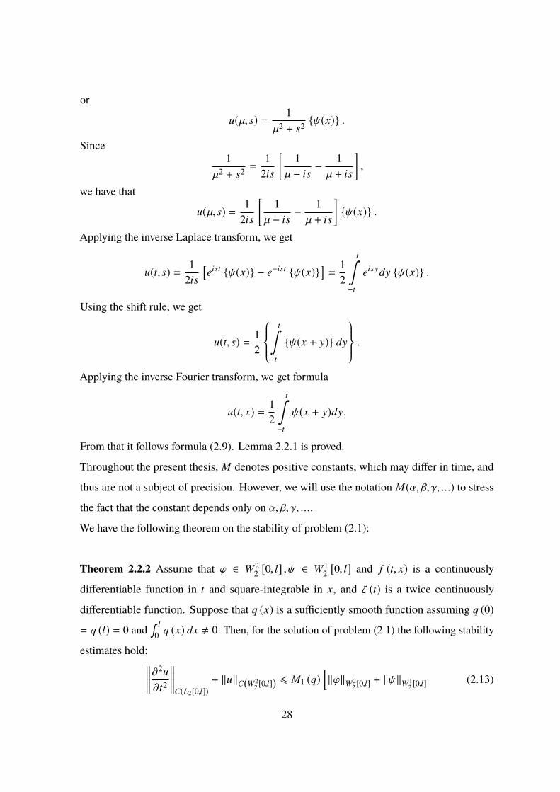
u(µ, s) =1

µ2 + s2 ψ(x) .

Since1

µ2 + s2 =1

2is

[1

µ − is−

1µ + is

],

we have that

u(µ, s) =1

2is

[1

µ − is−

1µ + is

]ψ(x) .

Applying the inverse Laplace transform, we get

u(t, s) =1

2is[eist ψ(x) − e−ist ψ(x)

]=

12

t∫−t

eisydy ψ(x) .

Using the shift rule, we get

u(t, s) =12

t∫

−t

ψ(x + y) dy .

Applying the inverse Fourier transform, we get formula

u(t, x) =12

t∫−t

ψ(x + y)dy.

From that it follows formula (2.9). Lemma 2.2.1 is proved.

Throughout the present thesis, M denotes positive constants, which may differ in time, and

thus are not a subject of precision. However, we will use the notation M(α, β, γ, ...) to stress

the fact that the constant depends only on α, β, γ, ....

We have the following theorem on the stability of problem (2.1):

Theorem 2.2.2 Assume that ϕ ∈ W22 [0, l] ,ψ ∈ W1

2 [0, l] and f (t, x) is a continuously

differentiable function in t and square-integrable in x, and ζ (t) is a twice continuously

differentiable function. Suppose that q (x) is a sufficiently smooth function assuming q (0)

= q (l) = 0 and∫ l0 q (x) dx , 0. Then, for the solution of problem (2.1) the following stability

estimates hold: ∂2u∂t2

C(L2[0,l])

+ ‖u‖C(W22 [0,l])

6 M1 (q)[‖ϕ‖W2

2 [0,l]+ ‖ψ‖W1

2 [0,l](2.13)

28

+ ‖ f (0, .)‖L2[0,l] +

∂ f∂t

C(L2[0,l])

+ ‖ζ ′′‖C[0,T]

],

‖p‖C[0,T] 6 M2 (q)[‖ϕ‖W2

2 [0,l]+ ‖ψ‖W1

2 [0,l]+ ‖ζ ′′‖C[0,T] (2.14)

+ ‖ f (0, .)‖L2[0,l] +

∂ f∂t

C(L2[0,l])

].

Proof. We will use the substitution

u (t, x) = w (t, x) + η (t) q (x) , (2.15)

where η (t) is the function defined by formula

η (t) =∫ t

0(t − s) p (s) ds, η (0) = η′ (0) = 0. (2.16)

It is easy to see that w (t, x) is the solution of the mixed problem

∂2w (t, x)∂t2 −

∂

∂x

(a (x)

∂w (t, x)∂x

)= f (t, x)

+η (t)[

ddx(a (x) q′ (x))

], x ∈ (0, l) , t ∈ (0,T) ,

w (0, x) = ϕ (x) ,wt (0, x) = ψ (x) , x ∈ [0, l] ,

w (t,0) = w (t, l) = 0, t ∈ [0,T] .

(2.17)

Now, we will take an estimate for |p (t)| . Applying the integral overdetermined condition∫ l0 u (t, x) dx = ζ (t) and substitution (2.15), we get

η (t) =ζ (t) −

∫ l0 w (t, x) dx∫ l

0 q (x) dx.

From that and p (t) = η′′ (t), it follows

p (t) =ζ ′′ (t) −

∫ l0∂2

∂t2w (t, x) dx∫ l0 q (x) dx

.

Then, using the Cauchy–Schwarz inequality and the triangle inequality, we obtain

|p (t)| 6|ζ ′′ (t)| +

∫ l0

∂2

∂t2w (t, x) dx∫ l

0 q (x) dx (2.18)

61∫ l

0 q (x) dx|ζ ′′ (t)| +

√l

(∫ l

0

(∂2w (t, x)∂t2

)2

dx

) 12

29

≤ M (q)

[|ζ ′′ (t)| +

∂2w (t, .)∂t2

L2[0,l]

]for all t ∈ [0,T] . From that, it follows

‖p‖C[0,T] 6 M (q)

[‖ζ ′′‖C[0,T] +

∂2w

∂t2

C(L2[0,l])

]. (2.19)

Now, using substitution (2.15), we get

∂2u (t, x)∂t2 =

∂2w (t, x)∂t2 + p (t) q (x) .

Applying the triangle inequality, we obtain ∂2u∂t2

C(L2[0,l])

6

∂2w

∂t2

C(L2[0,l])

+ ‖p‖C[0,T] ‖q‖L2[0,l] . (2.20)

Therefore, the proof of estimates (2.13) and (2.14) is based on equation (2.1), the triangle

inequality, estimates (2.19), (2.20) and on the stability estimate ∂2w

∂t2

C(L2[0,l])

6 M3(q,a)[‖ϕ‖W2

2 [0,l]+ ‖ψ‖W1

2 [0,l](2.21)

+ ‖ f (0, .)‖L2[0,l] +

∂ f∂t

C(L2[0,l])

+ ‖ζ ′′‖C[0,T]

],

for the solution of problem (2.17). This completes the proof of Theorem 2.2.2.

Now, we will prove the estimate (2.21) for the solution of problem (2.17).

Firstly, it is easy to see that problem (2.17) can be written as the abstract Cauchy problem

d2w (t)dt2 + Aw (t) = f (t) − η (t) Aq, t ∈ (0,T) , (2.22)

w (0) = ϕ,w′ (0) = ψ,

in a Hilbert space H with positive-definite self-adjoint operator A defined by formula (2.2).

Here,

w (t) = w(t, x), f (t) = f (t, x)

are unknown and known abstract functions defined on (0,T) with values in H = L2 [0, l] ,

respectively, and ϕ = ϕ(x),ψ = ψ(x),q = q(x) are given.

Secondly, applying the approaches of ( Ashyralyev and Sobolevskii, 2004) , we will prove a

30

lemma that will be needed in the sequel.

Lemma 2.2.3 Assume that ϕ ∈ D(A),ψ,q ∈ D(A12 ), f (t) is a continuously differentiable

abstract function in t with values in H, and η (t) is a twice continuously differentiable function

defined by formula (2.16). Then, for the solution of problem ( 2.22), the following stability

estimate holds d2w (t)dt2

H6 ‖Aϕ‖H +

A12ψ

H

(2.23)

+ ‖ f (0)‖H + T df

dt

C(H)+ M4(q)

∫ t

0|η′′(y)| dy

for any t ∈ [0,T] .

Proof. We have that (see Ashyralyev and Sobolevskii, 2004)

w (t) = c (t) ϕ + s (t)ψ +∫ t

0s (t − y) [ f (y) − η (y) Aq] dy, (2.24)

where

c (t) =eit A

12 + e−it A

12

2and s (t) = A−

12

eit A12− e−it A

12

2i.

Applying equation (2.22) and formula (2.24), we get

d2w (t)dt2 = f (t) − η (t) Aq − Ac (t) ϕ − As (t)ψ

−

∫ t

0As (t − y) [ f (y) − η (y) Aq] dy.

Integrating by parts, we get

d2w (t)dt2 = f (t) − η (t) Aq − Ac (t) ϕ − As (t)ψ − f (t)

+c (t) f (0) + η (t) Aq − c (t) η (0) Aq

+

∫ t

0c (t − y) f ′ (y) dy −

∫ t

0c (t − y) η′ (y) Aqdy.

Therefore,

d2w (t)dt2 = −Ac (t) ϕ − As (t)ψ + c (t) f (0)

+

∫ t

0c (t − y) f ′ (y) dy −

∫ t

0c (t − y) η′ (y) Aqdy.

31


d2w (t)dt2 = −Ac (t) ϕ − As (t)ψ + c (t) f (0) +

∫ t

0c (t − y) f ′ (y) dy

+ [s (t − y) η′ (y) Aq]t0 −∫ t

0s (t − y) η′′ (y) Aqdy

or

d2w (t)dt2 = −Ac (t) ϕ − As (t)ψ + c (t) f (0)

+

∫ t

0c (t − y) f ′ (y) dy −

∫ t

0s (t − y) η′′ (y) Aqdy

=

4∑i=1

Gi (t) ,

where

G1 (t) = c (t) ( f (0) − Aϕ) , G2 (t) = −As (t)ψ,

G3 (t) =∫ t

0c (t − y) f ′ (y) dy, G4 (t) = −

∫ t

0s (t − y) η′′(y)Aqdy

Now, applying the triangle inequality, we obtain d2w (t)dt2

H6

4∑i=1‖Gi (t)‖H

for any t ∈ [0,T] . Therefore, we will estimate ‖Gi (t)‖H , i = 1,2,3,4, separately. Firstly, using

the estimates (2.7), we obtain

‖G1 (t)‖H 6 ‖c (t)‖H→H ‖Aϕ − f (0)‖H 6 ‖Aϕ‖H + ‖ f (0)‖H ,

‖G2 (t)‖H = A

12 A

12 s (t)ψ

H6

A12 s (t)

H→H

A12ψ

H6

A12ψ

H

for any t ∈ [0,T] . Secondly, using the triangle inequality and estimates (2.7), we get

‖G3 (t)‖H ≤∫ t

0‖c (t − y)‖H→H ‖ f ′ (y)‖H dy 6

∫ t

0‖ f ′ (y)‖H dy

≤ t max0≤y≤t

‖ f ′ (y)‖H ≤ T max0≤y≤T

‖ f ′ (y)‖H = T df

dt

C(H)

for any t ∈ [0,T] . Thirdly, using the triangle inequality and estimates (2.7), we get

32

‖G4 (t)‖H ≤∫ t

0

A12 s (t − y)

H→H

A12 q

H|η′′(y)| dy

6

∫ t

0|η′′(y)| dy

A12 q

H≤ M4(q)

∫ t

0|η′′(y)| dy

for any t ∈ [0,T] . Combining these estimates, we obtain estimate (2.23) for the solution of

problem (2.22) for any t ∈ [0,T] .

Theorem 2.2.4 Assume that all conditions of Theorem 2.2.1 are satisfied. Then, for the

solution of problem (2.17) the stability estimate (2.21) holds.

Proof. Putting H = L2 [0, l] , ϕ = ϕ(x),ψ = ψ(x),q = q(x), f (t) = f (t, x) ,w (t) = w (t, x)

and applying estimates (2.18), (2.23), we get ∂2w (t)∂t2

L2[0,l]

6 M5 (a)[‖ϕ‖W2

2 [0,l]+ ‖ψ‖W1

2 [0,l]

]+ ‖ f (0, ·)‖L2[0,l] + T

∂ f∂t

C(L2[0,l])

+ M (q)M4 (q)

×

[∫ t

0|ζ ′′(y)| dy +

∫ t

0

∂2w (y, ·)

∂y2

L2[0,l]

dy

]for any t ∈ [0,T] . By the Gronwall’s inequality, we conclude that, for any t ∈ [0,T] , the

following estimate for the solution of problem (2.17) holds: ∂2w (t)∂t2

L2[0,l]

6M5 (a)

[‖ϕ‖W2

2 [0,l]+ ‖ψ‖W1

2 [0,l]

]+ ‖ f (0, ·)‖L2[0,l]

+ T

[ ∂ f∂t

C(L2[0,l])

+ M (q)M4 (q) ‖ζ ′′‖C[0,T]

]eM(q)M4(q)t .

This completes the proof of Theorem 2.2.4.

2.3 Stability of Difference Scheme

To formulate our results on a difference problem, we introduce the Banach space Cτ (H) =

C ([0,T]τ ,H) of all abstract grid functions φτ = φ (tk)Nk=0 defined on

[0,T]τ = tk = kτ,0 6 k 6 N,Nτ = T ,

with values in H, equipped with the norm

33

‖φτ‖Cτ(H) = max06k6N

‖φ (tk)‖H .

Moreover, L2h = L2 [0, l]h is the Hilbert space of all grid functions γh (x) = γnMn=0 defined

on

[0, l]h = xn = nh,0 6 n 6 M,Mh = l ,

equipped with the norm γh

L2h=

M∑

i=0|γi |

2 h

12

,

and W12h = W1

2 [0, l]h ,W22h = W2

2 [0, l]h are the discrete analogues of Sobolev spaces of all

grid functions γh (x) = γnMn=0 defined on [0, l]h with norms

γh

W12h=

M∑

i=0|γi |

2 h +M∑

i=1

γi − γi−1h

2 h

12

,

γh

W22h=

M∑

i=0|γi |

2 h +M−1∑i=1

γi+1 − 2γi + γi−1

h2

2 h

12

,

respectively. For the differential operator A defined by (2.2), we introduce the difference

operator Ah defined by formula

Ahϕh (x) =

−

1h

(a (xn+1)

ϕn+1 − ϕn

h− a (xn)

ϕn − ϕn−1h

)M−1

n=1,

acting in the space of grid functions ϕh (x) = ϕnMn=0 defined on [0, l]h, satisfying the

conditions ϕM = ϕ0 = 0.

It is easy that Ah is the self-adjoint positive-definite operator in H = L2h = L2 [0, l]h . Actually,

we have that ⟨Ahuh, vh⟩ = ∑

x∈[0,l]h

Ahuh(x)vh(x)h

= −

M−1∑n=1

1h

(a (xn+1)

un+1 − un

h− a (xn)

un − un−1h

)vnh

= −

M−1∑n=1

a (xn+1)un+1 − un

hvn +

M−1∑n=1

a (xn)un − un−1

hvn

= −

M∑n=2

a (xn)un − un−1

hvn−1 +

M−1∑n=1

a (xn)un − un−1

hvn

34

= −a (xM)uM − uM−1

hvM−1 −

M−1∑n=1

a (xn)un − un−1

hvn−1

+

M−1∑n=1

a (xn)un − un−1

hvn

=1h

a (xM) uM−1vM−1 +

M−1∑n=1

a (xn)un − un−1

hvn − vn−1

hh

= a (xM)uM − uM−1

hvM − vM−1

hh +

M−1∑n=1

a (xn)un − un−1

hvn − vn−1

hh

=

M∑n=1

a (xn)un − un−1

hvn − vn−1

hh,

⟨uh, Ahv

h⟩ = ∑x∈[0,l]h

uh(x)Ahvh(x)h

= −

M−1∑n=1

un1h

(a (xn+1)

vn+1 − vn

h− a (xn)

vn − vn−1h

)h

= −

M−1∑n=1

una (xn+1)vn+1 − vn

h+

M−1∑n=1

una (xn)vn − vn−1

h

= −

M∑n=2

un−1a (xn)vn − vn−1

h+

M−1∑n=1


h

= −uM−1a (xM)vM − vM−1

h−

M−1∑n=1

a (xn)vn − vn−1

hun−1

+

M−1∑n=1

a (xn) unvn − vn−1

h

=1h

a (xM) uM−1vM−1 +

M−1∑n=1

a (xn)un − un−1

hvn − vn−1

hh


hvM − vM−1

hh +

M−1∑n=1

a (xn)un − un−1

hvn − vn−1

hh

=

M∑n=1

a (xn)un − un−1

hvn − vn−1

hh,

From that it follows ⟨Ahuh, vh⟩ = ⟨

uh, Ahvh⟩35

and ⟨Ahuh,uh⟩ = M∑

n=1a (xn)

un − un−1h

un − un−1h

h (2.25)

≥ aM∑

n=1

un − un−1h

un − un−1h

h = a⟨Dhuh,Dhuh⟩ .

Here

Dhuh(x) =un − un−1

h

M

n=1.

Moreover, using the condition u0 = 0,we get

um =

m∑n=1

un − un−1h

h =m∑

i=1

um−i+1 − um−i

hh.

We will introduce the mesh function uh∗ (x) defined by the following formula

(um−i+1 − um−i

h

)∗=

um−i+1 − um−i

h,1 ≤ i ≤ m,1 ≤ m ≤ M,

0,otherwise.

Then

um =

M∑i=1


h

)∗

h.

Applying the discrete analogue of Minkowsky inequality and the definition of the mesh

function uh∗ (x), we get(M−1∑m=1

u2mh

) 12

≤

M∑i=1

(M−1∑m=1


h

)2

∗h

) 12

h

≤

M∑i=1

h

(M∑

n=1

(un − un−1h

)2h

) 12

= Mh

(M∑

n=1

(un − un−1h

)2h

) 12

= l

(M∑

n=1

(un − un−1h

)2h

) 12

.

Therefore, ⟨uh,uh⟩ = M−1∑

m=1u2

mh ≤ l2M∑

n=1

(un − un−1h

)2h (2.26)

= l2M∑

n=1

un − un−1h

un − un−1h

h = l2 ⟨Dhuh,Dhuh⟩ .

36

Applying inequalities (2.25) and (2.26), we get⟨Ahuh,uh⟩ ≥ a

l2

⟨uh,uh⟩ .

2.3.1 The first order of accuracy difference scheme

For the numerical solution

uknN

k=0

M

n=0of problem (2.1), we consider the first order of

accuracy difference scheme

uk+1n − 2uk

n + uk−1n

τ2 −

(a (xn+1)

uk+1n+1 − uk+1

n

h2 − a (xn)uk+1

n − uk+1n−1

h2

)= pk q (xn) + f (tk, xn) ,

tk = kτ, xn = nh,1 6 k 6 N − 1,1 6 n 6 M − 1,Nτ = T,

u0n = ϕ (xn) ,

u1n − u0

n

τ= ψ (xn) ,0 6 n 6 M,Mh = l,

uk+10 = uk+1

M = 0,∑M−1

i=1 uk+1i h = ζ (tk+1) ,−1 6 k 6 N − 1.

(2.27)

Here, it is assumed that qM = q0 = 0, and∑M−1

i=1 qi , 0.We have the following theorem on

the stability of the difference scheme (2.27):

Theorem 2.3.1 For the solution of difference scheme (2.27), the following stability esti-

mates hold:

uhk+1 − 2uh

k + uhk−1

τ2

N−1

k=1

Cτ(L2h)

+

uhk+1

N−1k=1

Cτ(W2

2h)(2.28)

6 M6 (q)[ ϕh

W2

2h+

ψh

W12h+

f h1

L2h

+

f hk − f h

k−1τ

N−1

k=2

Cτ(L2h)

+

ζk+1 − 2ζk + ζk−1

τ2

N−1

k=1

C[0,T]τ

, pkN−1k=1

C[0,T]τ

6 M7 (q)[ ϕh

W2

2h+

ψh

W22h+

f h1

L2h(2.29)

+

f hk − f h

k−1τ

N−1

k=2

Cτ(L2h)

+

ζk+1 − 2ζk + ζk−1

τ2

N−1

k=1

C[0,T]τ

.Here and throughout this subsection f h

k (x) = f (tk, xn)Mn=0 ,1 ≤ k ≤ N − 1.

37


ukn = wk

n + ηk qn, (2.30)

where

qn = q (xn) ,

and

ηk+1 =

k∑i=1(k + 1 − i) piτ

2,1 6 k 6 N − 1, η0 = η1 = 0. (2.31)

It is easy to see thatwk

nN

k=0

M

n=0is the solution of the difference problem

wk+1n − 2wk

n + wk−1n

τ2 −1h

(a (xn+1)

wk+1n+1 − w

k+1n

h− a (xn)

wk+1n − wk+1

n−1h

)= f (tk, xn) +

1h

[a (xn+1)

qn+1 − qn

h− a (xn)

qn − qn−1h

]ηk+1,

1 6 k 6 N − 1,1 6 n 6 M − 1,

w0n = ϕ (xn) ,

w1n − w

0n

τ= ψ (xn) ,0 6 n 6 M,

wk+10 = wk+1

M = 0,−1 6 k 6 N − 1.

(2.32)

Now, we will take an estimate for |pk | .Using the overdetermined condition∑M−1

i=1 uk+1i h =

ζ (tk+1) and substitution (2.30), one can obtain

ηk+1 =ζk+1 −

∑M−1i=1 wk+1

i h∑M−1i=1 qih

. (2.33)

Then, using the formulas pk =ηk+1−2ηk+ηk−1

τ2 and (2.33), we get

pk =ζk+1 − 2ζk + ζk−1 −

∑M−1i=1

(wk+1

i − 2wki + w

k−1i

)h

τ2 ∑M−1i=1 qih

.

Then, applying the discrete analogue of the Cauchy–Schwartz inequality and the triangle

inequality, we obtain

|pk | 61∑M−1

i=1 qih (2.34)

×

[ ζk+1 − 2ζk + ζk−1

τ2

+ M−1∑i=1

wk+1i − 2wk

i + wk−1i

τ2

h

]6

1∑M−1i=1 qih

ζk+1 − 2ζk + ζk−1

τ2

+ √l

wk+1

i − 2wki + w

k−1i

τ2

M

i=0

L2h

38

6 M8 (q)

[ ζk+1 − 2ζk + ζk−1

τ2

+ whk+1 − 2wh

k + whk−1

τ2

L2h

]for all 1 6 k 6 N − 1. From that, it follows

pkN−1k=1

C[0,T]τ

6 M8 (q) ζk+1 − 2ζk + ζk−1

τ2

N−1

k=1

C[0,T]τ

(2.35)

+

wh

k+1 − 2whk + w

hk−1

τ2

N−1

k=1

Cτ(L2h)

.Now, using substitution (2.30), we get

uk+1n − 2uk

n + uk−1n

τ2 =wk+1

n − 2wkn + w

k−1n

τ2 + pk q (xn) .

Applying the triangle inequality, we obtain

uhk+1 − 2uh

k + uhk−1

τ2

N−1

k=1

Cτ(L2h)

6

wh

k+1 − 2whk + w

hk−1

τ2

N−1

k=1

Cτ(L2h)

(2.36)

+ pk

N−1k=1

C[0,T]τ

q (xn)Mn=0

L2h

.


inequality, estimates (2.35), (2.36) and on the following stability estimate for the solution of

difference problem (2.32): wh

k+1 − 2whk + w

hk−1

τ2

N−1

k=1

Cτ(L2h)

6 M10(q)[ ϕh

W2

2h+

ψh

W12h

(2.37)

+ f h

1

L2h+

f hk − f h

k−1τ

N−1

k=2

Cτ(L2h)

+

ζk+1 − 2ζk + ζk−1

τ2

N−1

k=1

C[0,T]τ

.This completes the proof of Theorem 3.2.1.

Now, we will prove estimate (2.37) for the solution of difference problem (2.32). Firstly, it

is easy to see that difference scheme (2.32) can be written as the abstract Cauchy difference

problem wk+1 − 2wk + wk−1

τ2 + Awk+1 = fk − ηk+1 Aq,1 6 k 6 N − 1,

w0 = ϕ,w1 − w0

τ= ψ

(2.38)

39

in a Hilbert space H = L2h with positive-definite self-adjoint operator A. Here,

wkNk=0 =

wh

k

Nk=0 , fkN−1

k=1 =

f hk

N−1k=1

are unknown and known abstract mesh functions defined on [0,T]τ with values in H = L2h,

respectively, and ϕ = ϕh,ψ = ψh,q = qh are given elements.

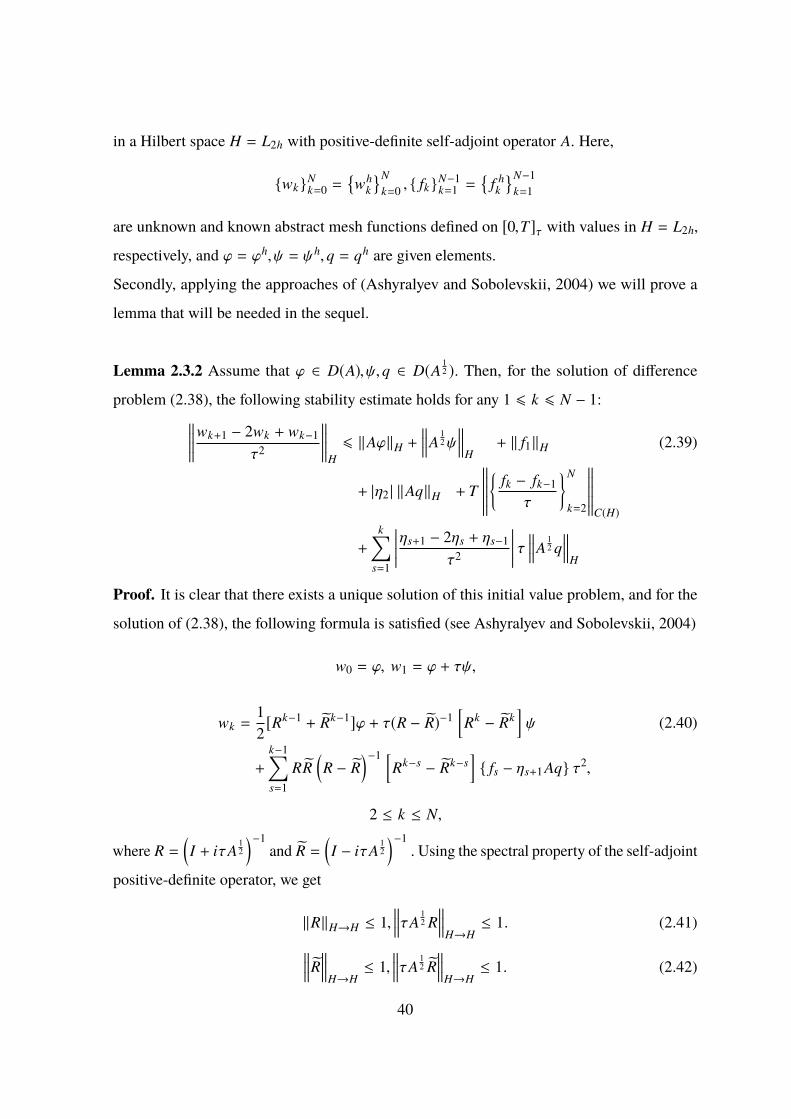
Secondly, applying the approaches of (Ashyralyev and Sobolevskii, 2004) we will prove a


Lemma 2.3.2 Assume that ϕ ∈ D(A),ψ,q ∈ D(A12 ). Then, for the solution of difference

problem (2.38), the following stability estimate holds for any 1 6 k 6 N − 1: wk+1 − 2wk + wk−1

τ2

H6 ‖Aϕ‖H +

A12ψ

H

+ ‖ f1‖H (2.39)

+ |η2 | ‖Aq‖H + T

fk − fk−1τ

N

k=2

C(H)

+

k∑s=1

ηs+1 − 2ηs + ηs−1

τ2

τ A12 q

H

Proof. It is clear that there exists a unique solution of this initial value problem, and for the

solution of (2.38), the following formula is satisfied (see Ashyralyev and Sobolevskii, 2004)

w0 = ϕ, w1 = ϕ + τψ,

wk =12[Rk−1 + Rk−1]ϕ + τ(R − R)−1

[Rk − Rk

]ψ (2.40)

+

k−1∑s=1

RR(R − R

)−1 [Rk−s − Rk−s

] fs − ηs+1 Aq τ2,

2 ≤ k ≤ N,

where R =(I + iτA

12

)−1and R =

(I − iτA

12

)−1.Using the spectral property of the self-adjoint

positive-definite operator, we get

‖R‖H→H ≤ 1, τA

12 R

H→H

≤ 1. (2.41) R

H→H≤ 1,

τA12 R

H→H

≤ 1. (2.42)

40

Now, we will establish estimates for wk+1−2wk+wk−1

τ2

H,1 ≤ k ≤ N − 1. Applying equation

(2.38) and formula (2.40), we get

wk+1 − 2wk + wk−1

τ2 (2.43)

= fk − ηk+1 Aq −12[Rk + Rk]Aϕ − τA(R − R)−1

[Rk+1 − Rk+1

]ψ

−

k∑s=1

ARR(R − R

)−1×

[Rk+1−s − Rk+1−s

] fs − ηs+1 Aq τ2

. = fk − ηk+1 Aq −12[Rk + Rk]Aϕ −

12i

[Rk R−1 − Rk R−1

]A

12ψ

+

(τA

12

2i

) (iτA

12

)−1

k∑s=1

Rk−s (I − R) +k∑

s=1Rk−s

(I − R

) fs − ηs+1 Aq

= fk − ηk+1 Aq −12[Rk + Rk]Aϕ −

12i

[Rk R−1 − Rk R−1

]A

12ψ

−12

k∑

s=1

[Rk−s − Rk+1−s] + k∑

s=1

[Rk−s − Rk+1−s

]( fs − ηs+1 Aq)

= fk − ηk+1 Aq −12[Rk + Rk]Aϕ −

12i

[Rk R−1 − Rk R−1

]A

12ψ (2.44)

−12

k∑

s=1

[Rk−s + Rk−s

]( fs − ηs+1 Aq) −

k∑s=1

[Rk+1−s − Rk+1−s

]( fs − ηs+1 Aq)

2 ≤ k ≤ N .

Applying Abel’s formula to (2.44), we can write

wk+1 − 2wk + wk−1

τ2

= fk − ηk+1 Aq −12[Rk + Rk]Aϕ −

12i

[Rk R−1 − Rk R−1

]A

12ψ

−12

k+1∑s=2

[Rk+1−s + Rk+1−s

]−

k∑s=1

[Rk+1−s + Rk+1−s

]( fs−1 − ηs Aq)

= fk − ηk+1 Aq −12[Rk + Rk]Aϕ −

12i

[Rk R−1 − Rk R−1

]A

12ψ

−12

k∑

s=2

[Rk+1−s + Rk+1−s

]( fs−1 − ηs Aq) + 2 ( fk − ηk+1 Aq)

−

k∑s=2

[Rk+1−s + Rk+1−s

]( fs − ηs+1 Aq) −

[Rk + Rk

]( f1 − η2 Aq)

41

= −12[Rk + Rk]Aϕ −

12i

[Rk R−1 − Rk R−1

]A

12ψ

−12

k∑s=2

[Rk+1−s + Rk+1−s

]( fs−1 − fs) +

12

[Rk + Rk

]f1

+12

k∑s=2

[Rk+1−s + Rk+1−s

](ηs − ηs+1) Aq −

12

[Rk + Rk

]η2 Aq,

Now, we have that

wk+1 − 2wk + wk−1

τ2

= −12[Rk + Rk]Aϕ −

12i

[Rk R−1 − R−1Rk

]A

12ψ

+12

[Rk + Rk

]f1 −

12

k∑s=2

[Rk+1−s − Rk+1−s

]( fs−1 − fs)

+12

k∑s=1

[Rk+1−s − Rk+1−s

](ηs − ηs+1) Aq

=

4∑i=1

Gi (k) ,2 ≤ k ≤ N,

where

G1 (k) = −12[Rk + Rk]Aϕ +

12[Rk + Rk] f1,

G2 (k) = −12i

[Rk R−1 − R−1Rk

]A

12ψ,

G3 (k) = −12

k∑s=2

[Rk+1−s + Rk+1−s

]( fs−1 − fs) ,

G4 (k) =12

k∑s=1

[Rk+1−s + Rk+1−s

](ηs − ηs+1) Aq.

Now, applying the triangle inequality, we obtain

‖G1 (k)‖H 612

[ Rk

H→H +

Rk

H→H

][‖Aϕ‖H + ‖ f1‖H]

≤ ‖Aϕ‖H + ‖ f1‖H ,

‖G2 (k)‖H 612

[ Rk R−1

H→H+

R−1Rk

H→H

] A12ψ

H

≤

A12ψ

H

42

for any 1 ≤ k ≤ N − 1. Secondly, using the triangle inequality and estimates (2.41), (2.42),

we get

‖G3 (k)‖H 6k∑

s=2

12

[ Rk+1−s

H→H +

Rk+1−s

H→H

]‖ fs−1 − fs‖H

6k∑

s=2‖ fs−1 − fs‖H ≤ T

fk − fk−1τ

N−1

k=1

Cτ(H)

for any 1 ≤ k ≤ N − 1. Thirdly, applying Abel’s formula to the sum G4 (k), we can write

G4 (k) =12

(iτA

12

)−1

k∑s=1

Rk−s (I − R) −k∑

s=1Rk−s

(I − R

)(ηs − ηs+1) Aq

=12

(iτA

12

)−1

k∑s=1

[Rk−s − Rk−s

](ηs − ηs+1) Aq

−

k∑s=1

[Rk+1−s − Rk+1−s

](ηs − ηs+1) Aq

=12

(iτA

12

)−1

k+1∑s=2

[Rk+1−s − Rk+1−s

](ηs−1 − ηs) Aq

−

k∑s=1

[Rk+1−s − Rk+1−s

](ηs − ηs+1) Aq

=12

(iτA

12

)−1

k∑s=1

[Rk+1−s − Rk+1−s

](ηs−1 − ηs) Aq

−

[Rk − Rk

](η0 − η1) Aq

−

k∑s=1

[Rk+1−s − Rk+1−s

](ηs − ηs+1) Aq

=

12

(iτA

12

)−1

k∑s=1

[Rk+1−s − Rk+1−s

](ηs−1 − 2ηs − ηs+1) Aq

=

(iτA

12

)−1 12

k∑

s=1

[Rk+1−s − Rk+1−s

] (ηs+1 − 2ηs + ηs−1

τ2

)τ2 Aq

Finally, using the triangle inequality and estimates (2.41), (2.42), we get

43

‖G4 (k)‖H 6k∑

s=1

12

[ Rk+1−s

H→H +

Rk+1−s

H→H

] ηs+1 − 2ηs + ηs−1

τ2

τ A12 q

H

6k∑

s=1

ηs+1 − 2ηs + ηs−1

τ2

τ A12 q

H

for any 1 ≤ k ≤ N − 1. Combining these estimates, we obtain estimate ( 2.39) for the solution

of problem (2.38) for any 1 ≤ k ≤ N − 1.

Theorem 2.3.3 For the solution of difference problem (2.32), the stability estimate ( 2.38)

holds.

Proof. Putting H = L2h, ϕ = ϕh,ψ = ψh,q = qh, Aϕ = Ahϕh,wk = wh

k , fk = f hk and

applying estimates (3.35) and (2.39), we get whk+1 − 2wh

k + whk−1

τ2

L2h

6 M12 (q)[ ϕh

W2

2h+

ψh

W12h

]+

f h1

L2h+ T

f hk − f h

k−1τ

N−1

k=2

Cτ(L2h)

+ M13 (q)M8 (q)

×

k∑s=1

[ ζs+1 − 2ζs + ζs−1

τ2

+ whs+1 − 2wh

s + whs−1

τ2

L2h

]τ

for any 1 ≤ k ≤ N − 1. By the difference analogue of Gronwall’s inequality, we conclude that whk+1 − 2wh

k + whk−1

τ2

L2h

61

1 − M13 (q)M8 (q) τ

M12 (q)

[ ϕh

W22h+

ψh

W12h

]+

f h1

L2h+ T

f hk − f h

k−1τ

N−1

k=2

Cτ(L2h)

+M13 (q)M8 (q)T

ζk+1 − 2ζk + ζk−1

τ2

N−1

k=1

C[0,T]τ

e(k−1)τ M13(q)M8(q)1−M13(q)M8(q)τ

for any 1 ≤ k ≤ N − 1.This completes the proof of Theorem 2.3.3.

44

2.3.2 The second order of accuracy difference scheme


uknN

k=0

M

n=0of problem (2.1), we consider the second order of


uk+1n − 2uk

n + uk−1n

τ2 −12h

(a (xn+1)

ukn+1 − uk

n

h− a (xn)

ukn − uk

n−1h

)−

14h

(a (xn+1)

uk+1n+1 − uk+1

n + uk−1n+1 − uk−1

n

h

−a (xn)uk+1

n − uk+1n−1 + uk−1

n − uk−1n−1

h

)= pk qn + f (tk, xn) ,

Nτ = T,1 6 n 6 M − 1,Mh = l, tk = kτ,1 6 k 6 N − 1,

u0n = ϕ (xn) ,0 6 n 6 M,

u1n − u0

n

τ−τ

h

(a (xn+1)

u1n+1 − u0

n+1 − u1n + u0

n

h

−a (xn)u1

n − u0n − u1

n−1 + u0n−1

h

)= ψ (xn) +

τ

2f (0, xn)

+τ

2

[1h

(a (xn+1)

u0n+1 − u0

n

h− a (xn)

u0n − u0

n−1h

)+ p0qn

],

1 6 n 6 M − 1,

uk+10 = uk+1

M = 0,∑M−1

i=1 uk+1i h = ζ (tk+1) ,−1 6 k 6 N − 1

(2.45)




Theorem 2.3.4 For the solution of difference scheme (2.45), the following stability estimates

hold:

uhk+1 − 2uh

k + uhk−1

τ2

N−1

k=1

Cτ(L2h)

+

uhk+1 + 2uh

k + uhk−1

4

N−1

k=1

Cτ(W2

2h)

(2.46)

6 M14 (q)[ ϕh

W2

2h+

ψh

W12h+

f h0

L2h

+

f hk − f h

k−1τ

N−1

k=1

Cτ(L2h)

+

ζk+1 − 2ζk + ζk−1

τ2

N−1

k=1

C[0,T]τ

, pkN−1k=1

C[0,T]τ

6 M15 (q)[ ϕh

W2

2h+

ψh

W22h+

f h0

L2h(2.47)

45

+

f hk − f h

k−1τ

N−1

k=1

Cτ(L2h)

+

ζk+1 − 2ζk + ζk−1

τ2

N−1

k=1

C[0,T]τ


k (x) = f (tk, xn)Mn=0 ,1 ≤ k ≤ N − 1.


ukn = wk

n + ηk qn, (2.48)

where

ηk =

k∑i=1

(k − i) pi + (k − (i − 1)) pi−1

2

τ2,1 6 k 6 N, η0 = 0, (2.49)


nN

k=0

M


wk+1n − 2wk

n + wk−1n

τ2 −12h

(a (xn+1)

wkn+1 − w

kn

h− a (xn)

wkn − w

kn−1

h

)−

14h

(a (xn+1)

wk+1n+1 − w

k+1n

h− a (xn)

wk+1n − wk+1

n−1h

)−

14h

(a (xn+1)

wk−1n+1 − w

k−1n

h− a (xn)

wk−1n − wk−1

n−1h

)= f (tk, xn)

+1h

[a (xn+1)

qn+1 − qn

h− a (xn)

qn − qn−1h

]×

14(ηk+1 + 2ηk + ηk−1) ,

1 6 k 6 N − 1,1 6 n 6 M − 1,

w0n = ϕ (xn) ,0 6 n 6 M,

w1n − w

0n

τ−τ

h

(a (xn+1)

w1n+1 − w

0n+1 − w

1n + w

0n

h

−a (xn)w1

n − w0n − w

1n−1 + w

0n−1

h

)−τ

h

(a (xn+1)

qn+1 − qn

h

−a (xn)qn − qn−1

h

)η1 = ψ (xn) +

τ

2f (0, xn)

+τ

2

[1h

(a (xn+1)

w0n+1 − w

0n

h− a (xn)

w0n − w

0n−1

h

)],

1 6 n 6 M − 1,

wk+10 = wk+1

M = 0,−1 6 k 6 N − 1.

(2.50)


i=1 uk+1i h =


46

ηk =ζk −

∑M−1i=1 wk

i h∑M−1i=1 qih

. (2.51)



pk =ζk+1 − 2ζk + ζk−1 −

∑M−1i=1

(wk+1

i − 2wki + w

k−1i

)h

τ2 ∑M−1i=1 qih

.

Then, applying the discrete analogue of the Cauchy–Schwarz inequality and the triangle


|pk | 61∑M−1

i=1 qih ×

[ ζk+1 − 2ζk + ζk−1

τ2

+ M−1∑i=1

wk+1i − 2wk

i + wk−1i

τ2

h

](2.52)

61∑M−1

i=1 qih

ζk+1 − 2ζk + ζk−1

τ2

+ √l

wk+1

i − 2wki + w

k−1i

τ2

M

i=0

L2h

6 M16 (q)

[ ζk+1 − 2ζk + ζk−1

τ2

+ whk+1 − 2wh

k + whk−1

τ2

L2h

]for all 1 6 k 6 N − 1. From that it follows pk

N−1k=1

C[0,T]τ

6 M16 (q) ζk+1 − 2ζk + ζk−1

τ2

N−1

k=1

C[0,T]τ

(2.53)

+

wh

k+1 − 2whk + w

hk−1

τ2

N−1

k=1

Cτ(L2h)


uk+1n − 2uk

n + uk−1n

τ2 =wk+1

n − 2wkn + w

k−1n

τ2 + pk q (xn) .


uhk+1 − 2uh

k + uhk−1

τ2

N−1

k=1

Cτ(L2h)

6

wh

k+1 − 2whk + w

hk−1

τ2

N−1

k=1

Cτ(L2h)

(2.54)

+ pk

N−1k=1

C[0,T]τ

q (xn)Mn=0

L2h

.


inequality, estimates (2.53), (2.54) and on the following stability estimate for the solution of

difference problem (2.50):

47

wh

k+1 − 2whk + w

hk−1

τ2

N−1

k=1

Cτ(L2h)

6 M17(q)[ ϕh

W2

2h+

ψh

W12h

(2.55)

+ f h

0

L2h+

f hk − f h

k−1τ

N−1

k=1

Cτ(L2h)

+

ζk+1 − 2ζk + ζk−1

τ2

N−1

k=1

C[0,T]τ

.

.This completes the proof of Theorem 2.3.4.

Now, we will prove estimate (2.55) for the solution of difference problem (2.50). Firstly, it

is easy to see that difference scheme (2.50) can be written as the abstract Cauchy difference

problem

wk+1 − 2wk + wk−1

τ2 + 14 A (wk+1 + 2wk + wk−1) = θk,

θk = fk − 14 (ηk+1 + 2ηk + ηk−1) Aq,

θk = θ(tk), tk = kτ,1 6 k 6 N − 1,Nτ = 1,(I + τ2 A

)τ−1 (w1 − w0) =

τ2 (θ0 − Aw0) + ψ,

θ0 = f (0) + p0q,w0 = ϕ,

(2.56)

in a Hilbert space H = L2h with positive-definite self-adjoint operator A. Here,

wkNk=0 =

wh

k

Nk=0 , fkN−1

k=1 =

f hk

N−1k=1

are unknown and known abstract mesh functions defined on [0,T]τ with values in H = L2h,

respectively, and ϕ = ϕh,ψ = ψh,q = qh are given elements.

Secondly, applying the approaches of ( Ashyralyev and Sobolevskii, 2004) ) we will prove a


Lemma 2.3.5 Assume that ϕ ∈ D(A),ψ,q ∈ D(A12 ). Then, for the solution of difference

problem (2.56), the following stability estimate holds for any 1 6 k 6 N − 1: wk+1 − 2wk + wk−1

τ2

H6 M (q)

[‖Aϕ‖H +

A12ψ

H+ ‖ f0‖H + |η1 | (2.57)

+

fk − fk−1τ

N

k=1

C(H)

+

k∑s=1

ηs+1 − 2ηs + ηs−1

τ2

τfor any 1 6 k 6 N − 1.

48

Proof. It is clear that there exists a unique solution of this initial value problem, and for the

solution of (2.56), the following formula is satisfied (see Ashyralyev and Sobolevskii, 2004)

w0 = ϕ,w1 =(I + τ2 A

)−1[(

I +τ2

2A)ϕ + τψ +

τ2

2θ0

](2.58)

wk =

[Rk +

12i

A−12

(I −

iτA12

2

) [Rk − Rk

]×

((I +

iτA12

2

)τ

2A − iA

12

(I + τ2 A

)) (I + τ2 A

)−1]ϕ

+i2

A−12

(I −

iτA12

2

) [Rk − Rk

] (I + τ2 A

)−1(I +

iτA12

2

)ψ

+i2

A−12

(I −

iτA12

2

) [Rk − Rk

] (I + τ2 A

)−1(I +

iτA12

2

)τ

2θ0

−

k−1∑s=1

τ

2iA−

12

[Rk−s − Rk−s

]θs,

2 ≤ k ≤ N .

Applying Abel’s formula, we can write

wk =

Rk −

12

iA−12 B

[Rk − Rk

] (Bτ

2A − iA

12

(I + τ2 A

)) (I + τ2 A

)−1ϕ (2.59)

+

i2

A−12 BB

[Rk − Rk

] (I + τ2 A

)−1ψ

+

i2

A−12 BB

[Rk − Rk

] (I + τ2 A

)−1τ

2θ0

+A−1

2

k−1∑s=2

[BRk−s − BRk−s

](θs−1 − θs)

,

+A−1

2

[B + B

]θk−1 −

[BRk−1 − BRk−1

]θ1

,

2 ≤ k ≤ N,

where

R = BB−1 =

(I −

iτA12

2

) (I +

iτA12

2

)−1

R = BB−1 =

(I +

iτA12

2

) (I −

iτA12

2

)−1

.

49

Using the spectral property of the self-adjoint positive-definite operator, we get

‖R‖H→H ≤ 1, R

H→H

≤ 1,

(I ±

iτA12

2

)−1

H→H

≤ 1, (2.60)

(I ± iτA12

)−1

H→H≤ 1,

τA12

(I ± iτA

12

)−1

H→H≤ 1. (2.61)

Now, we will establish estimates for wk+1−2wk+wk−1

τ2

H,1 ≤ k ≤ N − 1. Applying equation (

2.56), formula (2.59) and identities

I + R = 2B−1, I + R = 2B−1, (2.62)

we get

Awk+1 + wk + wk−1

4(2.63)

=

B−1Rk B−1 −

14

iτA12

[BRk−1B−1 − B−1Rk−1B

]×

(I + τ2 A

)−1−

12

[B−1Rk − B−1Rk−1

]Aϕ

+12


] (I + τ2 A

)−1

iA12ψ

+14

iτA

12


] (I + τ2 A

)−1θ0

+12

k−1∑s=2

[B−1Rk−s + B−1Rk−s

](θs−1 − θs) +

14

[τ2 AB−1B−1

]θk

+12

[B−1 + B−1

]θk−1 −

12

[B−1Rk−1 + B−1Rk−1

]θ1

=

4∑i=1

Ji (k) ,

where

J1 (k) =

B−1Rk B−1 −14

iτA12


] (I + τ2 A

)−1

−12

[B−1Rk − B−1Rk−1

]Aϕ,

J2 (k) =12


] (I + τ2 A

)−1

iA12ψ,

J3 (k) =14

iτA

12


] (I + τ2 A

)−1θ0

50

+14

[τ2 AB−1B−1

]θk +

12

[B−1 + B−1

]θk−1

−12

[B−1Rk−1 + B−1Rk−1

]θ1,

J4 (k) =12

k−1∑s=2

[B−1Rk−s + B−1Rk−s

](θs−1 − θs) .

Now, applying the triangle inequality, we obtain Awk+1 + wk + wk−1

4

H6

4∑i=1‖Ji (k)‖H (2.64)

for any 1 ≤ k ≤ N − 1. Therefore, we will estimate ‖Ji (k)‖H , i = 1,2,3,4, separately. Firstly,

using estimates (2.60), (2.61), we get

‖J1 (k)‖H 6 B−1Rk B−1

H→H

+14

[ iτA12 BRk−1B−1

(I + τ2 A

)−1

H→H

+

iτA12 B−1Rk−1B

(I + τ2 A

)−1

H→H

]+

12

[ B−1Rk

H→H+

B−1Rk−1

H→H

]‖Aϕ‖H

≤ M ‖Aϕ‖H ,

‖J2 (k)‖H 612

[ BRk−1B−1(I + τ2 A

)−1

H→H

+

B−1Rk−1B(I + τ2 A

)−1

H→H

A12ψ

H

]≤ M

A12ψ

H

for any 1 ≤ k ≤ N − 1. Secondly, using the triangle inequality and estimates (2.60), (2.61),

we get

‖J3 (k)‖H 614

[ BRk−1B−1τA12

(I + τ2 A

)−1

H→H

+

B−1Rk−1BτA12

(I + τ2 A

)−1

H→H

]‖θ0‖H

+14

[ τ2 AB−1B−1

H→H‖θk ‖H

]+

12

[ B−1 H→H +

B−1

H→H

]‖θk−1‖H

+12

[ B−1Rk−1

H→H+

B−1Rk−1

H→H

]‖θ1‖H

51

≤114

[‖θ0‖H +

k∑i=1‖θi − θi−1‖H

],

‖J4 (k)‖H 6k−1∑s=2

12

[ B−1Rk−s

H→H+

B−1Rk−s

H→H

]‖θs−1 − θs‖H

6k−1∑s=2‖θs−1 − θs‖H

for any 1 ≤ k ≤ N − 1. Using the triangle inequality and estimate (2.64), we get

A wk+1 + 2wk + wk−1

4

H≤ M ‖Aϕ‖H + M

A12ψ

H+

k−1∑s=2‖θs−1 − θs‖H (2.65)

+114

[‖θ0‖H +


]for any 1 ≤ k ≤ N − 1.Using the triangle inequality and estimate, we get wk+1 − 2wk + wk−1

τ2

H≤ A

wk+1 + 2wk + wk−14

H+ ‖θk ‖H

≤ M ‖Aϕ‖H + M A

12ψ

H+

k−1∑s=2‖θs−1 − θs‖H

+154

[‖θ0‖H +


]for any 1 ≤ k ≤ N − 1. Combining these estimates, we obtain estimate ( 2.57) for the solution

of difference problem (2.56) for any 1 ≤ k ≤ N − 1.

Theorem 2.3.6 For the solution of difference problem (2.50), the stability estimate (2.56)

holds.

Proof. Putting H = L2h, ϕ = ϕh,ψ = ψh,q = qh, Aϕ = Ahϕh,wk = wh

k , fk = f hk and

applying estimates (2.52) and (2.57), we get whk+1 − 2wh

k + whk−1

τ2

L2h

6 M20 (q)[ ϕh

W2

2h+

ψh

W12h

]

+ f h

0

L2h+ T

f hk − f h

k−1τ

N−1

k=1

Cτ(L2h)

+ M21 (q)M16 (q)

×

k∑s=1

[ ζs+1 − 2ζs + ζs−1

τ2

+ whs+1 − 2wh

s + whs−1

τ2

L2h

]τ

52

for any 1 ≤ k ≤ N − 1. By the difference analogue of Gronwall’s inequality, we conclude that whk+1 − 2wh

k + whk−1

τ2

L2h

61

1 − M21 (q)M16 (q) τ

M20 (q)

[ ϕh

W22h+

ψh

W12h

]+

f h0

L2h+ T

f hk − f h

k−1τ

N−1

k=1

Cτ(L2h)

+ M21 (q)M16 (q)T

×

ζk+1 − 2ζk + ζk−1

τ2

N−1

k=1

C[0,T]τ

e(k−1)τ M21(q)M16(q)1−M21(q)M16(q)τ

for any 1 ≤ k ≤ N − 1.This completes the proof of Theorem 2.3.6.

Applying same approach with this work we can study another the second order of accuracy

difference scheme for the numerical solution of problem (2.1).

uk+1n − 2uk

n + uk−1n

τ2 −12h

(a (xn+1)

uk+1n+1 − uk+1

n + uk−1n+1 − uk−1

n

h

−a (xn)uk+1

n − uk+1n−1 + uk−1

n − uk−1n−1

h

)= pk qn + f (tk, xn) ,qn = q (xn) , xn = nh,Nτ = T,

1 6 n 6 M − 1,Mh = l, tk = kτ,1 6 k 6 N − 1,

u0n = ϕ (xn) ,0 6 n 6 M,

u1n − u0

n

τ−τ

h

(a (xn+1)

u1n+1 − u0

n+1 − u1n + u0

n

h

−a (xn)u1

n − u0n − u1

n−1 + u0n−1

h

)+ ψ (xn) +

τ

2f (0, xn)

+τ

2

[1h

(a (xn+1)

u0n+1 − u0

n

h− a (xn)

u0n − u0

n−1h

)+ p0qn

],

1 6 n 6 M − 1,

uk+10 = uk+1

M = 0,∑M−1

i=1 uk+1i h = ζ (tk+1) ,−1 6 k 6 N − 1

(2.66)





hold:

uhk+1 − 2uh

k + uhk−1

τ2

N−1

k=1

Cτ(L2h)

+

uhk+1 + uh

k−12

N−1

k=1

Cτ(W2

2h)

53

6 M14 (q)[ ϕh

W2

2h+

ψh

W12h+

f h0

L2h

+

f hk − f h

k−1τ

N−1

k=1

Cτ(L2h)

+

ζk+1 − 2ζk + ζk−1

τ2

N−1

k=1

C[0,T]τ

, pkN−1k=1

C[0,T]τ

6 M15 (q)[ ϕh

W2

2h+

ψh

W22h+

f h0

L2h

+

f hk − f h

k−1τ

N−1

k=1

Cτ(L2h)

+

ζk+1 − 2ζk + ζk−1

τ2

N−1

k=1

C[0,T]τ

.Now, we consider one more the second order of accuracy difference scheme

uk+1n − 2uk

n + uk−1n

τ2 −1h

(a (xn+1)

ukn+1 − uk

n

h− a (xn)

ukn − uk

n−1h

)+τ2

4

1h

a (xn+1)1h

[1h

(a (xn+2)

uk+1n+2 − uk+1

n+1h

− a (xn+1)uk+1

n+1 − uk+1n

h

)−

1h

(a (xn+1)

ukn+1 − uk

n

h− a (xn)

ukn − uk

n−1h

)]−

1h

a (xn)

[1h

(a (xn+1)

ukn+1 − uk

n

h− a (xn−)

ukn − uk

n−1h

)−

1h

(a (xn)

uk+1n − uk+1

n−2h

− a (xn−1)uk+1

n−1 − uk+1n−2

h

)]= pk qn + f (tk, xn) ,qn = q (xn) , xn = nh,Nτ = T,

1 6 n 6 M − 1,Mh = l, tk = kτ,1 6 k 6 N − 1,

u0n = ϕ (xn) ,0 6 n 6 M,

u1n − u0

n

τ−τ

h

(a (xn+1)

u1n+1 − u0

n+1 − u1n + u0

n

h

−a (xn)u1

n − u0n − u1

n−1 + u0n−1

h

)+ ψ (xn) +

τ

2f (0, xn)

+τ

2

[1h

(a (xn+1)

u0n+1 − u0

n

h− a (xn)

u0n − u0

n−1h

)+ p0qn

],

1 6 n 6 M − 1,

uk+10 = uk+1

M = 0,∑M−1

i=1 uk+1i h = ζ (tk+1) ,−1 6 k 6 N − 1

(2.67)



54



hold:

uhk+1 − 2uh

k + uhk−1

τ2

N−1

k=1

Cτ(L2h)

+

uhk

N−1k=1

Cτ(W2

2h)

6 M14 (q)[ ϕh

W2

2h+

ψh

W12h+

f h0

L2h

+

f hk − f h

k−1τ

N−1

k=1

Cτ(L2h)

+

ζk+1 − 2ζk + ζk−1

τ2

N−1

k=1

C[0,T]τ

, pkN−1k=1

C[0,T]τ

6 M15 (q)[ ϕh

W2

2h+

ψh

W22h+

f h0

L2h

+

f hk − f h

k−1τ

N−1

k=1

Cτ(L2h)

+

ζk+1 − 2ζk + ζk−1

τ2

N−1

k=1

C[0,T]τ

.

2.4 Numerical Experiments

In this section, we study the numerical solution of the identification problem

∂2u (t, x)∂t2 −

∂2u (t, x)∂x2 = p (t) sin x + e−t sin x,

x ∈ (0, π) , t ∈ (0,1) ,

u (0, x) = sin x,ut (0, x) = − sin x, x ∈ [0, π] ,

u (t,0) = u (t, π) = 0, t ∈ [0,1] ,∫ π

0 u (t, x) dx = 2e−t, t ∈ [0,1]

(2.68)

for a hyperbolic differential equation. The exact solution pair of this problem is (u (t, x) , p (t)) =(e−t sin x, e−t ) .Firstly, for the numerical solution of problem (2.68), we present the following first order of

accuracy difference scheme for the approximate solution for problem (2.68):

55

uk+1n − 2uk

n + uk−1n

τ2 −uk+1

n+1 − 2uk+1n + uk+1

n−1h2

= pk sin xn + e−tk+1 sin xn,

tk = kτ, xn = nh,1 6 k 6 N − 1,1 6 n 6 M − 1,

u0n = sin xn,

u1n − u0

n

τ= − sin xn,0 6 n 6 M,Mh = π,Nτ = 1,

uk+10 = uk+1

M = 0,∑M−1

i=1 uk+1i h = 2e−tk+1,−1 6 k 6 N − 1.

(2.69)

The algorithm for obtaining the solution of identification problem (2.69) contains three stages.

Actually, let us define

ukn = wk

n + ηk sin xn,0 ≤ k ≤ N,0 ≤ n ≤ M, (2.70)

Applying difference scheme (2.69) and formula (2.70), we will obtain

ηk+1 =2e−tk+1 −

∑M−1i=1 wk+1

i h∑M−1i=1 sin xih

,−1 ≤ k ≤ N − 1 (2.71)

and

wk+1n − 2wk

n + wk−1n

τ2 −wk+1

n+1 − 2wk+1n + wk+1

n−1h2

+

∑M−1i=1 wk+1


sin xn2(cos h − 1)

h2

=

[2∑M−1

i=1 sin xih

2(cos h − 1)h2 + 1

]e−tk+1 sin xn,

1 6 k 6 N − 1,1 6 n 6 M − 1,

w0n = sin xn,

w1n − w

0n

τ= − sin xn,0 6 n 6 M,

wk+10 = wk+1

M = 0,−1 6 k 6 N − 1.

(2.72)

In the first stage, we find the solutionwk

nN

k=0

M

n=0of the corresponding first order of accuracy

difference scheme (2.72). For obtaining it, we will write difference scheme (2.72) in matrix

form as Awk+1 + Bwk + Cwk−1 = ϕk,1 6 k 6 N − 1,

w0 = sin xnMn=0 ,w

1 = (1 − τ) sin xnMn=0 ,

(2.73)

56

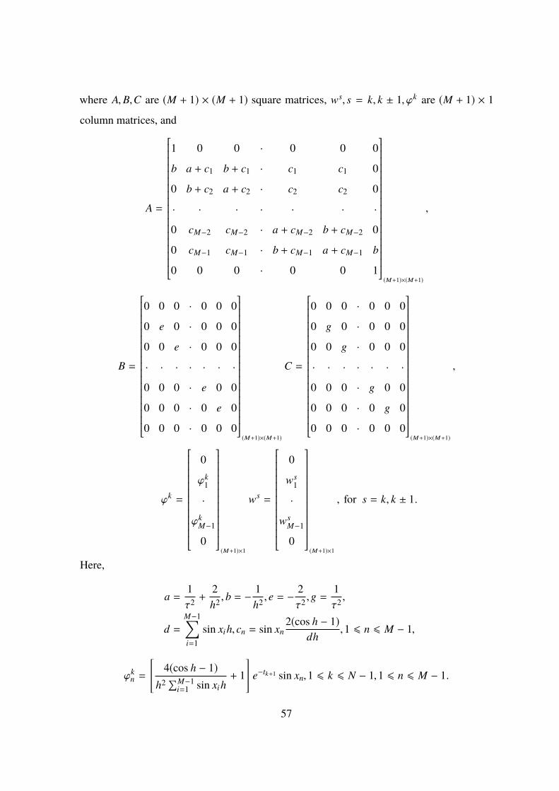
where A,B,C are (M + 1) × (M + 1) square matrices, ws, s = k, k ± 1, ϕk are (M + 1) × 1

column matrices, and

A =

1 0 0 · 0 0 0

b a + c1 b + c1 · c1 c1 0

0 b + c2 a + c2 · c2 c2 0

· · · · · · ·

0 cM−2 cM−2 · a + cM−2 b + cM−2 0

0 cM−1 cM−1 · b + cM−1 a + cM−1 b

0 0 0 · 0 0 1

(M+1)×(M+1)

,

B =

0 0 0 · 0 0 0

0 e 0 · 0 0 0

0 0 e · 0 0 0

· · · · · · ·

0 0 0 · e 0 0

0 0 0 · 0 e 0

0 0 0 · 0 0 0

(M+1)×(M+1)

C =

0 0 0 · 0 0 0

0 g 0 · 0 0 0

0 0 g · 0 0 0

· · · · · · ·

0 0 0 · g 0 0

0 0 0 · 0 g 0

0 0 0 · 0 0 0

(M+1)×(M+1)

,

ϕk =

0

ϕk1

·

ϕkM−1

0

(M+1)×1

ws =

0

ws1

·

wsM−1

0

(M+1)×1

, for s = k, k ± 1.

Here,

a =1τ2 +

2h2 , b = −

1h2 , e = −

2τ2 ,g =

1τ2 ,

d =M−1∑i=1

sin xih, cn = sin xn2(cos h − 1)

dh,1 6 n 6 M − 1,

ϕkn =

[4(cos h − 1)

h2 ∑M−1i=1 sin xih

+ 1

]e−tk+1 sin xn,1 6 k 6 N − 1,1 6 n 6 M − 1.

57

So, we have the initial value problem for the second-order difference equation (2.73) with

respect to k with the matrix coefficients A,B and C. Since w0and w1are given, we can obtainwk

nN

k=0

M

n=0by (2.73).

Now, applying formula (2.31), we can obtain

pk =ηk+1 − 2ηk + ηk−1

τ2 ,1 ≤ k ≤ N − 1. (2.74)

In the second stage, we will obtain pkN−1k=1 by formulas (2.71) and (2.74). Finally, in the third

stage, we will obtain

uknN

k=0

M

n=0by formulas (2.70) and (2.71). The errors are computed by

Eu = max06k6N

(M−1∑n=1

u (tk, xn) − ukn

2 h

) 12

,

Ep = max16k6N−1

|p (tk) − pk | ,

where u (t, x) , p(t) represent the exact solution, ukn represents the numerical solutions at (tk, xn)

and pk represents the numerical solutions at tk . The numerical results are given in Table 1.

Table 1: Error analysis for difference scheme (2.69)

Error N =M = 20 N =M = 40 N =M = 80 N =M = 160

Eu 0.0347 0.0181 0.0092 0.0047

Ep 0.0462 0.0240 0.0123 0.0062

As can be seen in Table 1, if N and M are doubled, the value of errors between the exact

solution and approximate solution decreases by a factor of approximately 12 for the first order

difference scheme (2.69).

58

Secondly, for the numerical solution of problem (2.68), we present the following second order

of accuracy difference schemes for the approximate solution for problem (2.68):

uk+1n − 2uk

n + uk−1n

τ2 −12

ukn+1 − 2uk

n + ukn−1

h2

−14

[uk+1

n+1 − 2uk+1n + uk+1

n−1h2 +

uk−1n+1 − 2uk−1

n + uk−1n−1

h2

]= pk sin xn + e−tk sin xn,

tk = kτ,1 6 k 6 N − 1,Nτ = 1, xn = nh,1 6 n 6 M − 1,Mh = π,

u0n = sin xn,

u1n − u0

n

τ−τ

h2

(u1

n+1 − u0n+1 − 2u1

n + 2u0n + u1

n−1 − u0n−1

)= − sin xn +

τ

2

(u0

n+1 − 2u0n + u0

n−1h2 + p0 sin xn + sin xn

),0 6 n 6 M,

uk+10 = uk+1

M = 0,∑M−1

i=1 uk+1i h = 2e−tk+1,−1 6 k 6 N − 1

(2.75)

and

uk+1n − 2uk

n + uk−1n

τ2 −12

[uk+1

n+1 − 2uk+1n + uk+1

n−1h2 +

uk−1n+1 − 2uk−1

n + uk−1n−1

h2

]= pk sin xn + e−tk sin xn,

tk = kτ,1 6 k 6 N − 1,Nτ = 1, xn = nh,1 6 n 6 M − 1,Mh = π,

u0n = sin xn,

u1n − u0

n

τ−τ

h2

(u1

n+1 − u0n+1 − 2u1

n + 2u0n + u1

n−1 − u0n−1

)= − sin xn +

τ

2

(u0

n+1 − 2u0n + u0

n−1h2 + p0 sin xn + sin xn

),0 6 n 6 M,

uk+10 = uk+1

M = 0,∑M−1

i=1 uk+1i h = 2e−tk+1,−1 6 k 6 N − 1

(2.76)



ukn = wk

n + ηk sin xn,0 ≤ k ≤ N,0 ≤ n ≤ M, (2.77)

Applying the second order of accuracy difference scheme(2.75) and formula (2.77), we will

obtain

ηk =2e−tk −

∑M−1i=1 wk


,0 ≤ k ≤ N (2.78)

and the difference scheme

59

wk+1n − 2wk

n + wk−1n

τ2 −12wk

n+1 − 2wkn + w

kn−1

h2

−14

[wk+1

n+1 − 2wk+1n + wk+1

n−1h2 +

wk−1n+1 − 2wk−1

n + wk−1n−1

h2

]+

12(cos h − 1)

h2 ∑M−1i=1 sin xih

sin xn

×

(∑M−1i=1 wk+1

i h + 2∑M−1

i=1 wki h +

∑M−1i=1 wk−1

i h)

= e−tk sin xn +[e−tk+1 + 2e−tk + e−tk−1

] (cos h − 1)h2 ∑M−1

i=1 sin xihsin xn

1 6 k 6 N − 1,1 6 n 6 M − 1,

w0n = sin xn,0 6 n 6 M,

w1n − w

0n

τ−τ

h2(w1

n+1 − 2w1n + w

1n−1

)+

2τ(cosh−1)h2 ∑M−1

i=1 sin xihsin xn

∑M−1i=1 w1

i h

+τ

2h2

(w0

n+1 − 2w0n + w

0n−1

)=

(τ2− 1

)sin xn

+4τe−t1(cosh−1)h2 ∑M−1

i=1 sin xihsin xn,0 6 n 6 M,

wk+10 = wk+1

M = 0,−1 6 k 6 N − 1.

(2.79)


nN

k=0

M

n=0of the corresponding second order of

accuracy difference scheme (2.79). For obtaining it, we will write difference scheme (2.79),

in matrix form as Awk+1 + Bwk + Cwk−1 = ϕk,1 6 k 6 N − 1,

w0,w1 are given,(2.80)


column matrices and

A =

1 0 0 · 0 0 0

b a + c1 b + c1 · c1 c1 c1

0 b + c2 a + c2 · c2 c2 c2

· · · · · · ·

0 cM−2 cM−2 · a + cM−2 b + cM−2 0

0 cM−1 cM−1 · b + cM−1 a + cM−1 b

0 0 0 · 0 0 1

(M+1)×(M+1)

,

60

B =

0 0 0 · 0 0 0

r q + e1 r + e1 · e1 e1 e1

0 r + e2 q + e2 · e2 e2 e2

· · · · · · ·

0 eM−2 eM−2 · q + eM−2 r + eM−2 0

0 eM−1 eM−1 · r + eM−1 q + eM−1 r

0 0 0 · 0 0 0

(M+1)×(M+1)

,

C =

0 0 0 · 0 0 0

b a + c1 b + c1 · c1 c1 0

0 b + c2 a + c2 · c2 c2 0

· · · · · · ·

0 cM−2 cM−2 · a + cM−2 b + cM−2 0

0 cM−1 cM−1 · b + cM−1 a + cM−1 b

0 0 0 · 0 0 0

(M+1)×(M+1)

,

ϕk =

0

ϕk1

·

ϕkM−1

0

(M+1)×1

, ws =

0

ws1

·

wsM−1

0

(M+1)×1

, for s = k, k ± 1,

w0 =

sin x0

sin x1

·

sin xM−1

sin xM

,

61

where,

a =1τ2 +

12h2 , b = −

14h2 ,r = −

12h2 ,q =

1h2 −

2τ2 ,

cn =12

sin xn(cos h − 1)

dh, en = sin xn

(cos h − 1)dh

,

d =M−1∑i=1

sin xih,1 6 n 6 M − 1,

ϕkn = e−tk sin xn +

(e−tk+1 + 2e−tk + e−tk−1

) (cos h − 1)h2 ∑M−1

i=1 sin xihsin xn,

1 6 k 6 N − 1,1 6 n 6 M − 1.

Finally, we obtain w1.Applying the formula

w1n − w

0n

τ−τ

h2(w1

n+1 − 2w1n + w

1n−1

)+

2τ(cos h − 1)h2 ∑M−1

i=1 sin xihsin xn

∑M−1i=1 w1

i h

+τ

2h2

(w0

n+1 − 2w0n + w

0n−1

)=

(τ2− 1

)sin xn +

4τe−t1(cos h − 1)h2 ∑M−1

i=1 sin xihsin xn,

and conditions w10 = w1

M = 0,we get

Ew1 + Fw0 = γ. (2.81)

Here

E =

1 0 0 · 0 0 0

y x + z1 y + z1 · z1 z1 0

0 y + z2 x + z2 · z2 z2 0

· · · · · · ·

0 zM−2 zM−2 · x + zM−2 y + zM−2 0

0 zM−1 zM−1 · y + zM−1 x + zM−1 y

0 0 0 · 0 0 1

(M+1)×(M+1)

,

62

x = −2τh2 +

1τ, y = −

τ

h2 , zn =2τ(cos h − 1)

dhsin xn,

u = −τ

2h2 , v =1τ+τ

h2 , v = −32τ−

2τh2 + 1,

F =

0 0 0 · 0 0 0

u v u · 0 0 0

0 u v · 0 0 0

· · · · · · ·

0 0 0 · v u 0

0 0 0 · u v u

0 0 0 · 0 0 0

(M+1)×(M+1)

,

γ =

0

∇1

·

∇M−1

0

(M+1)×1

,

∇n =

(τ

2− 1 +

4τe−t1(cos h − 1)h2 ∑M−1

i=1 sin xih

)sin xn.

From that, it follows

w1 = E−1(γ − Fw0

). (2.82)



nN

k=0

M

n=0by (2.80)


pk =ηk+1 − 2ηk + ηk−1

τ2 ,1 ≤ k ≤ N − 1, p0 =2τ2η1 (2.83)



uknN

k=0

M

n=0by formulas (2.77) and (2.78).

63

In the same manner, we obtain algorithm for obtaining the solution of identification problem

(2.76) ukNk=0 =

uk

nN

k=0

M

n=0and pk

N−1k=1 by three stages. The errors are computed by

Eu = max06k6N

(M−1∑n=1

u (tk, xn) − ukn

2 h

) 12

,

Ep = max16k6N−1

|p (tk) − pk | ,

where u (t, x) , p(t) represent the exact solution, ukn represents the numerical solutions at

(tk, xn), and pk represents the numerical solutions at tk . The numerical results are given in the

following Tables 2 and 3.

Table 2:Error analysis for difference scheme (2.75)

Error N =M = 20 N =M = 40 N =M = 80 N =M = 160

Eu 0.0016 4.2029e − 04 1.0648e − 04 2.6796e − 05

Ep 0.0027 7.0457e − 04 1.7835e − 04 4.4867e − 05


Error N =M = 20 N =M = 40 N =M = 80 N =M = 160

Eu 0.0016 4.2011e − 04 1.0647e − 04 2.6795e − 05

Ep 0.0033 8.5650e − 04 2.1690e − 04 5.4570e − 05

As can be seen in Tables 2 and 3, if N and M are doubled, the value of errors between the exact

solution and approximate solution decreases by a factor of approximately 14 for the second

order difference schemes (2.75) and (2.76), respectively.

64

CHAPTER 3

STABILITY OF THE HYPERBOLIC DIFFERENTIAL AND DIFFERENCE

EQUATIONWITH NONLOCAL CONDITIONS

3.1 Introduction In this chapter, we consider the source identification problem for a

one-dimensional hyperbolic equation with nonlocal conditions

∂2u (t, x)∂t2 −

∂

∂x

(a (x)

∂u (t, x)∂x

)+ δu(t, x)

= p (t) q (x) + f (t, x) , x ∈ (0, l) , t ∈ (0,T) ,

u (0, x) = ϕ (x) ,ut (0, x) = ψ (x) , x ∈ [0, l] ,

u (t,0) = u (t, l) ,ux (t,0) = ux (t, l) ,∫ l0 u (t, x) dx = ζ (t) , t ∈ [0,T] ,

(3.1)

where u (t, x) and p (t) are unknown functions, a (x) ≥ a > 0,a (l) = a (0) , δ > 0,

f (t, x) , ζ (t) , ϕ (x) and ψ (x) are given sufficiently smooth functions and q (x) is a given

sufficiently smooth function assuming q (0) = q (l) , q′ (0) = q′ (l) and∫ l0 q (x) dx , 0.

3.2 Stability of the Differential Problem (3.1)

To formulate our results, we introduce the differential operator A defined by the formula

Au = −ddx

(a (x)

du (x)dx

)+ δu(x) (3.2)

with the domain

D (A) = u : u,u′′ ∈ L2 [0, l] ,u (0) = u (l) ,u′ (0) = u′ (l) .

It is easy that A is the self-adjoint positive-definite operator in H = L2 [0, l] . Actually, for all

u, v ∈ L2 [0, l] we have that

〈Au, v〉 =∫ l

0A(u)v (x) dx =

∫ l

0

[−

ddx

(a (x)

du (x)dx

)+ δu(x)

]v (x) dx

= −

(a (x)

du (x)dx

)v(x)

l0+

∫ l

0a (x)

du (x)dx

dv (x)dx

dx

+δ

∫ l

0u(x)v (x) dx

65

= −a (l)du (l)

dxv(l) + a (0)

du (0)dx

v(0) +∫ l

0a (x)

du (x)dx

dv (x)dx

dx

+δ

∫ l

0u(x)v (x) dx

Since

a (l) = a (0) ,u (0) = u (l) ,u′ (0) = u′ (l) , (3.3)

we have that

−a (l)du (l)

dxv(l) + a (0)

du (0)dx

v(0) = 0.

Therefore,

〈Au, v〉 =∫ l

0a (x)

du (x)dx

dv (x)dx

dx + δ∫ l

0u(x)v (x) dx.

Using (3.3), we get

〈u, Av〉 =∫ l

0u (x) A(v)dx =

∫ l

0u (x)

[−

ddx

(a (x)

dv (x)dx

)+ δv(x)

]dx

= − u(x)(a (x)

dv (x)dx

)l0+

∫ l

0a (x)

dv (x)dx

du (x)dx

dx

+δ

∫ l

0v(x)u (x) dx

= −u(l)a (l)dv (l)

dx+ u(0)a (0)

dv (0)dx

+

∫ l

0a (x)

dv (x)dx

du (x)dx

dx

=

∫ l

0a (x)

dv (x)dx

du (x)dx

dx + δ∫ l

0v(x)u (x) dx.


〈Au, v〉 = 〈u, Av〉

and

〈Au,u〉 =∫ l

0a (x)

du (x)dx

du (x)dx

dx + δ∫ l

0u(x)u (x) dx (3.4)

≥ δ

∫ l

0u(x)u (x) dx

= δ 〈u,u〉 .

We have the following theorem on the stability of problem (3.1).

66

Theorem 3.2.1 Assume that ϕ ∈ W22 [0, l] ,ψ ∈ W1

2 [0, l] and f (t, x) is a continuously

differentiable function in t and square integrable in x, and ζ (t) is a twice continuously

differentiable function. Suppose that q (x) is a sufficiently smooth function assuming q (0)

= q (l), q′ (0) = q′ (l) and∫ l0 q (x) dx , 0. Then, for the solution of problem (3.1), the

following stability estimates hold: ∂2u∂t2

C(L2[0,l])

+ ‖u‖C(W22 [0,l])

6 K1 (q)[‖ϕ‖W2

2 [0,l]+ ‖ψ‖W1

2 [0,l](3.5)

+ ‖ f (0, .)‖L2[0,l] +

∂ f∂t

C(L2[0,l])

+ ‖ζ ′′‖C[0,T]

],

‖p‖C[0,T] 6 K2 (q)[‖ϕ‖W2

2 [0,l]+ ‖ψ‖W1

2 [0,l]+ ‖ζ ′′‖C[0,T] (3.6)

+ ‖ f (0, .)‖L2[0,l] +

∂ f∂t

C(L2[0,l])

].

Proof. We will use the following substitution

u (t, x) = w (t, x) + η (t) q (x) , (3.7)

where η (t) is the function defined by formula

η (t) =∫ t

0(t − s) p (s) ds, η (0) = η′ (0) = 0. (3.8)

It is easy to see that w (t, x) is the solution of problem

∂2w (t, x)∂t2 −

∂

∂x

(a (x)

∂w (t, x)∂x

)+ δw(t, x)

= f (t, x) + η (t)[

ddx(a (x) q′ (x)) − δq (x)

],

x ∈ (0, l) , t ∈ (0,T) ,

w (0, x) = ϕ (x) ,wt (0, x) = ψ (x) , x ∈ [0, l] ,

w (t,0) = w (t, l) ,wx (t,0) = wx (t, l) , t ∈ [0,T] .

(3.9)

Applying the integral overdetermined condition∫ l0 u (t, x) dx = ζ (t) and substitution (3.7),

we get

η (t) =ζ (t) −

∫ l0 w (t, x) dx∫ l

0 q (x) dx.

67

From that and p (t) = η′′ (t) it follows

p (t) =ζ ′′ (t) −

∫ l0

∂2

∂t2w (t, x) dx∫ l0 q (x) dx

.

Applying∫ l0 q (x) dx , 0,we get estimate

|p (t)| ≤ K3 (q)

[|ζ ′′ (t)| +

∂2w (t, .)∂t2

L2[0,l]

](3.10)

for all t ∈ [0,T] . From that it follows

‖p‖C[0,T] 6 K3 (q)

[‖ζ ′′‖C[0,T] +

∂2w

∂t2

C(L2[0,l])

]. (3.11)


∂2u (t, x)∂t2 =

∂2w (t, x)∂t2 + p (t) q (x) .

Applying the triangle inequality, we obtain ∂2u∂t2

C(L2[0,l])

6

∂2w

∂t2

C(L2[0,l])

+ ‖p‖C[0,T] ‖q‖L2[0,l] . (3.12)


inequality, estimates (3.11), (3.12) and on the following stability estimate ∂2w

∂t2

C(L2[0,l])

6 K4(q,a)[‖ϕ‖W2

2 [0,l]+ ‖ψ‖W1

2 [0,l](3.13)

+ ‖ f (0, .)‖L2[0,l] +

∂ f∂t

C(L2[0,l])

+ ‖ζ ′′‖C[0,T]

],

for the solution of problem (3.9). It was proved in Section 2.2 for the identification hyperbolic

problem with local boundary condition. The proof of (3.13) is carried out according to the

same approach. This completes the proof of Theorem 3.2.1.

3.3 Stability of the Difference Scheme

To formulate our results for the differential operator A defined by (3.2), we introduce the

difference operator Ah defined by the formula

Ahϕh (x) =

−

1h

(a (xn+1)

ϕn+1 − ϕn

h− a (xn)

ϕn − ϕn−1h

)+ δϕn

M−1

n=1,

68

acting in the space of grid functions ϕh (x) = ϕnMn=0 defined on [0, l]h satisfying the

conditions ϕ0 = ϕM , ϕ1 − ϕ0 = ϕM − ϕM−1.

It is easy that Ah is the self-adjoint positive-definite operator in H = L2h = L2 [0, l]h . Actually,

we have that ⟨Ahuh, vh⟩ = ∑

x∈[0,l]h

Ahuh(x)vh(x)h

=

M−1∑n=1

[−

1h

(a (xn+1)

un+1 − un

h− a (xn)

un − un−1h

)+ δun

]vnh

= −

M−1∑n=1

a (xn+1)un+1 − un

hvn +

M−1∑n=1

a (xn)un − un−1

hvn + δ

M−1∑n=1

unvnh

= −

M∑n=2

a (xn)un − un−1

hvn−1 +

M−1∑n=1

a (xn)un − un−1

hvn + δ

M−1∑n=1

unvnh

= −a (xM)uM − uM−1

hvM−1 + a (x1)

u1 − u0h

v0

−

M−1∑n=2

a (xn)un − un−1

hvn−1 +

M−1∑n=2

a (xn)un − un−1

hvn + δ

M−1∑n=1

unvnh

= −a (xM)uM − uM−1

hvM + a (x1)

u1 − u0h

v0

+

M∑n=2

a (xn)un − un−1

hvn − vn−1

hh + δ

M−1∑n=1

unvnh.

Since

a (xM) = a (x1) , ϕ0 = ϕM, ϕ1 − ϕ0 = ϕM − ϕM−1, (3.14)

we have that

−a (xM)uM − uM−1

hvM + a (x1)

u1 − u0h

v0 = 0.

⟨Ahuh, vh⟩ = M∑

n=2a (xn)

un − un−1h

vn − vn−1h

h + δM−1∑n=1

unvnh.

Using (3.14), we get ⟨uh, Ahv

h⟩ = ∑x∈[0,l]h

uh(x)Ahvh(x)h

69

=

M−1∑n=1

un

[−

1h

(a (xn+1)

vn+1 − vn

h− a (xn)

vn − vn−1h

)+ δvn

]h

= −

M−1∑n=1

una (xn+1)vn+1 − vn

h+

M−1∑n=1


h+ δ

M−1∑n=1

unvnh

= −

M∑n=2

un−1a (xn)vn − vn−1

h+

M−1∑n=1


h+ δ

M−1∑n=1

unvnh

= −uM−1a (xM)vM − vM−1

h+ u1a (x1)

v1 − v0h−

M−1∑n=2

a (xn)vn − vn−1

hun−1

+

M−1∑n=2

a (xn) unvn − vn−1

hh + δ

M−1∑n=1

unvnh


hvM − vM−1

h+

M−1∑n=2

a (xn)un − un−1

hvn − vn−1

hh

+δ

M−1∑n=1

unvnh

=

M∑n=2

a (xn)un − un−1

hvn − vn−1

hh + δ

M−1∑n=1

unvnh.

From that it follows ⟨Ahuh, vh⟩ = ⟨

uh, Ahvh⟩

and ⟨Ahuh,uh⟩ = M∑

n=2a (xn)

un − un−1h

un − un−1h

h + δM−1∑n=1

ununh

≥ δ

M−1∑n=1

ununh

= δ⟨uh,uh⟩ .

3.3.1 The first order of accuracy difference scheme


uknN

k=0

M

n=0of problem (3.1), we consider the first order of


70

uk+1n − 2uk

n + uk−1n

τ2 −

(a (xn+1)

uk+1n+1 − uk+1

n

h2 − a (xn)uk+1

n − uk+1n−1

h2

)+δuk+1

n = pk q (xn) + f (tk, xn) , tk = kτ, xn = nh,

1 6 k 6 N − 1,1 6 n 6 M − 1,Nτ = T,

u0n = ϕ (xn) ,

u1n − u0

n

τ= ψ (xn) ,0 6 n 6 M,Mh = l,

uk+10 = uk+1

M ,uk+11 − uk+1

0 = uk+1M − uk+1

M−1,∑M−1i=1 uk+1

i h = ζ (tk+1) ,−1 6 k 6 N − 1.

(3.15)

Here, it is assumed that

q0 = qM,q1 − q0 = qM − qM−1

and∑M−1

i=1 qi , 0.We have the following theorem on the stability of difference scheme (3.15).

Theorem 3.3.1 For the solution of difference scheme (3.15)

uhk+1 − 2uh

k + uhk−1

τ2

N−1

k=1

Cτ(L2h)

+

uhk+1

N−1k=1

Cτ(W2

2h)(3.16)

6 M5 (q)[ ϕh

W2

2h+

ψh

W12h+

f h1

L2h

+

f hk − f h

k−1τ

N−1

k=2

Cτ(L2h)

+

ζk+1 − 2ζk + ζk−1

τ2

N−1

k=1

C[0,T]τ

, pkN−1k=1

C[0,T]τ

6 M6 (q)[ ϕh

W2

2h+

ψh

W22h+

f h1

L2h(3.17)

+

f hk − f h

k−1τ

N−1

k=2

Cτ(L2h)

+

ζk+1 − 2ζk + ζk−1

τ2

N−1

k=1

C[0,T]τ


k (x) = f (tk, xn)Mn=0 ,1 ≤ k ≤ N − 1.

Proof. We will use the following substitution

ukn = wk

n + ηk qn, (3.18)

where

qn = q (xn) ,

71

and

ηk+1 =

k∑i=1(k + 1 − i) piτ

2,1 6 k 6 N − 1, η0 = η1 = 0. (3.19)


nN

k=0

M

n=0is the solution of difference problem

wk+1n − 2wk

n + wk−1n

τ2 −1h

(a (xn+1)

wk+1n+1 − w

k+1n

h− a (xn)

wk+1n − wk+1

n−1h

)+δwk+1

n = f (tk, xn) +1h

[a (xn+1)

qn+1 − qn

h− a (xn)

qn − qn−1h

− δhqn

]ηk+1,

1 6 k 6 N − 1,1 6 n 6 M − 1,

w0n = ϕ (xn) ,

w1n − w

0n

τ= ψ (xn) ,0 6 n 6 M,

wk+10 = wk+1

M ,wk+11 − wk+1

0 = wk+1M − wk+1

M−1,−1 6 k 6 N − 1.

(3.20)

Applying the overdetermined condition∑M−1

i=1 uk+1i h = ζ (tk+1) and substitution ( 3.18), one

can obtain that

ηk+1 =ζk+1 −

∑M−1i=1 wk+1

i h∑M−1i=1 qih

. (3.21)

Then, using formulas pk =ηk+1 − 2ηk + ηk−1


pk =ζk+1 − 2ζk + ζk−1 −

∑M−1i=1

(wk+1

i − 2wki + w

k−1i

)h

τ2 ∑M−1i=1 qih

.

|pk | 6 K7 (q)

[ ζk+1 − 2ζk + ζk−1

τ2

+ whk+1 − 2wh

k + whk−1

τ2

L2h

](3.22)

for all 1 6 k 6 N − 1. From that it follows

pkN−1k=1

C[0,T]τ

≤ K7 (q) ζk+1 − 2ζk + ζk−1

τ2

N−1

k=1

C[0,T ]τ

+

wh

k+1 − 2whk + w

hk−1

τ2

N−1

k=1

Cτ(L2h)

. (3.23)


uk+1n − 2uk

n + uk−1n

τ2 =wk+1

n − 2wkn + w

k−1n

τ2 + pk q (xn) .

72


uk+1i − 2uk

i + uk−1i

τ2

N−1

k=1

M

n=0

Cτ(L2h)

(3.24)

6

wk+1

i − 2wki + w

k−1i

τ2

N−1

k=1

M

n=0

Cτ(L2h)

+ pk

N−1k=1

C[0,T]τ

q (xn)M−1n=1

L2h

.


inequality, estimates (3.23), (3.24) and on the following stability estimate wh

k+1 − 2whk + w

hk−1

τ2

N−1

k=1

Cτ(L2h)

(3.25)

6 K8(q)[ ϕh

W2

2h+

ψh

W12h+

f h1

L2h

+

f hk − f h

k−1τ

N−1

k=2

Cτ(L2h)

+

ζk+1 − 2ζk + ζk−1

τ2

N−1

k=1

C[0,T]τ

for the solution of difference problem (3.20). It was proved in Section 2.3 for the identification

hyperbolic problemwith local boundary condition. The proof of (3.25) is carried out according

to the same approach. This completes the proof of Theorem 3.3.1.

3.3.2 The second order of accuracy difference scheme

We have the following approximate formulas

−u(2h) + 4u(h) − 3u(0)2h

− ux(0) = o(h2),

3u(l) − 4u(l − h) + u(l − 2h)2h

− ux(l) = o(h2).

(3.26)

Applying (3.26) for the numerical solution

uknN

k=0

M

n=0of problem (3.1), we consider the

second order of accuracy difference scheme

73

uk+1n − 2uk

n + uk−1n

τ2 −12h

(a (xn+1)

ukn+1 − uk

n

h− a (xn)

ukn − uk

n−1h

)−

14h

(a (xn+1)

uk+1n+1 − uk+1

n + uk−1n+1 − uk−1

n

h

−a (xn)uk+1

n − uk+1n−1 + uk−1

n − uk−1n−1

h

)+

12δuk

n + δuk+1

n + uk−1n

4

= pk qn + f (tk, xn) , xn = nh, tk = kτ,

Nτ = T,1 6 n 6 M − 1,Mh = l, tk = kτ,1 6 k 6 N − 1,

u0n = ϕ (xn) ,0 6 n 6 M,

u1n − u0

n

τ−τ

h

(a (xn+1)

u1n+1 − u0

n+1 − u1n + u0

n

h

−a (xn)u1

n − u0n − u1

n−1 + u0n−1

h+ δh(u0

n − u1n)

)= ψ (xn) +

τ

2[ f (0, xn) + p0qn]

−τ

2

[−

1h

(a (xn+1)

u0n+1 − u0

n

h− a (xn)

u0n − u0

n−1h

)+ δu0

n

],1 6 n 6 M − 1,

uk+10 = uk+1

M ,−uk+12 + 4uk+1

1 − 3uk+10 = 3uk+1

M − 4uk+1M−1 + uk+1

M−2,∑M−1i=1 uk+1

i h = ζ (tk+1) ,−1 6 k 6 N − 1

(3.27)

Here, it is assumed that

qM = q0,−q2 + 4q1 − 3q0 = 3qM − 4qM−1 + qM−2 (3.28)

and∑M−1

i=1 qi , 0.We have the following theorem on the stability of the difference scheme

(3.27):


hold:

uhk+1 − 2uh

k + uhk−1

τ2

N−1

k=1

Cτ(L2h)

+

uhk+1 + 2uh

k + uhk−1

4

N−1

k=1

Cτ(W2

2h)

(3.29)

6 M9 (q)[ ϕh

W2

2h+

ψh

W12h+

f h0

L2h

+

f hk − f h

k−1τ

N−1

k=1

Cτ(L2h)

+

ζk+1 − 2ζk + ζk−1

τ2

N−1

k=1

C[0,T]τ

, pkN−1k=1

C[0,T]τ

6 M10 (q)[ ϕh

W2

2h+

ψh

W22h+

f h0

L2h(3.30)

74

+

f hk − f h

k−1τ

N−1

k=1

Cτ(L2h)

+

ζk+1 − 2ζk + ζk−1

τ2

N−1

k=1

C[0,T]τ


k (x) = f (tk, xn)Mn=0 ,1 ≤ k ≤ N − 1.


ukn = wk

n + ηk qn, (3.31)

where

ηk =

k∑i=1

(k − i) pi + (k − (i − 1)) pi−1

2

τ2,1 6 k 6 N, η0 = 0, (3.32)


nN

k=0

M


wk+1n − 2wk

n + wk−1n

τ2 −12h

(a (xn+1)

wkn+1 − w

kn

h− a (xn)

wkn − w

kn−1

h

)−

14h

(a (xn+1)

wk+1n+1 − w

k+1n + wk−1

n+1 − wk−1n

h

−a (xn)wk+1

n − wk+1n−1 + w

k−1n − wk−1

n−1h

)+

12δwk

n + δwk+1

n + wk−1n

4

=1h

[a (xn+1)

qn+1 − qn

h− a (xn)

qn − qn−1h

− δhqn

] 14(ηk+1 + 2ηk + ηk−1)

+ f (tk, xn) ,1 6 k 6 N − 1,1 6 n 6 M − 1,

w0n = ϕ (xn) ,0 6 n 6 M,

w1n − w

0n

τ−τ

h

(a (xn+1)

w1n+1 − w

0n+1 − w

1n + w

0n

h

−a (xn)w1

n − w0n − w

1n−1 + w

0n−1

h+ δh(w0

n − w1n)

)−τ

h

(a (xn+1)

qn+1 − qn

h

−a (xn)qn − qn−1

h− δhqn

)η1 = ψ (xn) +

τ

2f (0, xn)

−τ

2

[−

1h

(a (xn+1)

w0n+1 − w

0n

h− a (xn)

w0n − w

0n−1

h

)+ δw0

n

],1 6 n 6 M − 1,

wk+10 = wk+1

M ,−wk+12 + 4wk+1

1 − 3wk+10 = 3wk+1

M − 4wk+1M−1 + w

k+1M−2,

−1 6 k 6 N − 1.

(3.33)


i=1 uk+1i h =

75


ηk =ζk −

∑M−1i=1 wk

i h∑M−1i=1 qih

. (3.34)



pk =ζk+1 − 2ζk + ζk−1 −

∑M−1i=1

(wk+1

i − 2wki + w

k−1i

)h

τ2 ∑M−1i=1 qih

.

Then, applying the discrete analogue of the Cauchy–Schwarz inequality and the triangle


|pk | 6 M11 (q)

[ ζk+1 − 2ζk + ζk−1

τ2

+ whk+1 − 2wh

k + whk−1

τ2

L2h

](3.35)

for all 1 6 k 6 N − 1. From that, it follows

pkN−1k=1

C[0,T]τ

6 K11 (q) ζk+1 − 2ζk + ζk−1

τ2

N−1

k=1

C[0,T]τ

(3.36)

+

wh

k+1 − 2whk + w

hk−1

τ2

N−1

k=1

Cτ(L2h)


uk+1n − 2uk

n + uk−1n

τ2 =wk+1

n − 2wkn + w

k−1n

τ2 + pk q (xn) .


uhk+1 − 2uh

k + uhk−1

τ2

N−1

k=1

Cτ(L2h)

6

wh

k+1 − 2whk + w

hk−1

τ2

N−1

k=1

Cτ(L2h)

(3.37)

+ pk

N−1k=1

C[0,T]τ

q (xn)Mn=0

L2h

.


inequality, estimates (3.36), (3.37) and on the following stability estimate wh

k+1 − 2whk + w

hk−1

τ2

N−1

k=1

Cτ(L2h)

6 M12(q)[ ϕh

W2

2h+

ψh

W12h

(3.38)

76

+ f h

0

L2h+

f hk − f h

k−1τ

N−1

k=1

Cτ(L2h)

+

ζk+1 − 2ζk + ζk−1

τ2

N−1

k=1

C[0,T]τ

.

.for the solution of difference problem (3.33). It was proved in Section 2.3 for the identification

hyperbolic problemwith local boundary condition. The proof of (3.38) is carried out according

to the same approach. This completes the proof of Theorem 3.3.2.

Applying ( 3.26) and same approach with this work we can study another the second order of


uk+1n − 2uk

n + uk−1n

τ2 −12h

(a (xn+1)

uk+1n+1 − uk+1

n + uk−1n+1 − uk−1

n

h

−a (xn)uk+1

n − uk+1n−1 + uk−1

n − uk−1n−1

h

)+ δ

uk+1n + uk−1

n

2

= pk qn + f (tk, xn) ,qn = q (xn) , xn = nh,Nτ = T,

1 6 n 6 M − 1,Mh = l, tk = kτ,1 6 k 6 N − 1,

u0n = ϕ (xn) ,0 6 n 6 M,

u1n − u0

n

τ−τ

h

(a (xn+1)

u1n+1 − u0

n+1 − u1n + u0

n

h

−a (xn)u1

n − u0n − u1

n−1 + u0n−1

h+ δh(u0

n − u1n)

)= ψ (xn) +

τ

2[ f (0, xn) + p0qn]

−τ

2

[−

1h

(a (xn+1)

u0n+1 − u0

n

h− a (xn)

u0n − u0

n−1h

)+ δu0

n

],1 6 n 6 M − 1,

uk+10 = uk+1

M ,−uk+12 + 4uk+1

1 − 3uk+10 = 3uk+1

M − 4uk+1M−1 + uk+1

M−2,∑M−1i=1 uk+1

i h = ζ (tk+1) ,−1 6 k 6 N − 1

(3.39)

Here, it is assumed that the formula (3.28) holds and∑M−1

i=1 qi , 0.We have the following

theorem on the stability of the difference scheme (3.39):


hold:

uhk+1 − 2uh

k + uhk−1

τ2

N−1

k=1

Cτ(L2h)

+

uhk+1 + uh

k−12

N−1

k=1

Cτ(W2

2h)

6 M14 (q)[ ϕh

W2

2h+

ψh

W12h+

f h0

L2h

77

+

f hk − f h

k−1τ

N−1

k=1

Cτ(L2h)

+

ζk+1 − 2ζk + ζk−1

τ2

N−1

k=1

C[0,T]τ

, pkN−1k=1

C[0,T]τ

6 M15 (q)[ ϕh

W2

2h+

ψh

W22h+

f h0

L2h

+

f hk − f h

k−1τ

N−1

k=1

Cτ(L2h)

+

ζk+1 − 2ζk + ζk−1

τ2

N−1

k=1

C[0,T]τ

.

Now, we consider one more the second order of accuracy difference scheme

uk+1n − 2uk

n + uk−1n

τ2 −1h

(a (xn+1)

ukn+1 − uk

n

h− a (xn)

ukn − uk

n−1h

)+ δuk

n

+τ2

4

1h

a (xn+1)1h

[1h

(a (xn+2)

uk+1n+2 − uk+1

n+1h

− a (xn+1)uk+1

n+1 − uk+1n

h

)−

1h

(a (xn+1)

ukn+1 − uk

n

h− a (xn)

ukn − uk

n−1h

)]−

1h

a (xn)

[1h

(a (xn+1)

ukn+1 − uk

n

h− a (xn−)

ukn − uk

n−1h

)−

1h

(a (xn)

uk+1n − uk+1

n−2h

− a (xn−1)uk+1

n−1 − uk+1n−2

h

)]−2δ

1h

(a (xn+1)

uk+1n+1 − uk+1

n

h− a (xn)

uk+1n − uk+1

n−1h

)+ δ2uk+1

n

= pk qn + f (tk, xn) ,qn = q (xn) , xn = nh,Nτ = T,

1 6 n 6 M − 1,Mh = l, tk = kτ,1 6 k 6 N − 1,

u0n = ϕ (xn) ,0 6 n 6 M,

u1n − u0

n

τ−τ

h

(a (xn+1)

u1n+1 − u0

n+1 − u1n + u0

n

h

−a (xn)u1

n − u0n − u1

n−1 + u0n−1

h+ δh(u0

n − u1n)

)= ψ (xn) +

τ

2[ f (0, xn) + p0qn]

−τ

2

[−

1h

(a (xn+1)

u0n+1 − u0

n

h− a (xn)

u0n − u0

n−1h

)+ δu0

n

],1 6 n 6 M − 1,

uk+10 = uk+1

M ,−uk+12 + 4uk+1

1 − 3uk+10 = 3uk+1

M − 4uk+1M−1 + uk+1

M−2,∑M−1i=1 uk+1

i h = ζ (tk+1) ,−1 6 k 6 N − 1

(3.40)

78

Here, it is assumed that formula (3.28) holds and∑M−1

i=1 qi , 0.We have the following theorem

on the stability of the difference scheme (3.40):


hold:

uhk+1 − 2uh

k + uhk−1

τ2

N−1

k=1

Cτ(L2h)

+

uhk

N−1k=1

Cτ(W2

2h)

6 M14 (q)[ ϕh

W2

2h+

ψh

W12h+

f h0

L2h

+

f hk − f h

k−1τ

N−1

k=1

Cτ(L2h)

+

ζk+1 − 2ζk + ζk−1

τ2

N−1

k=1

C[0,T]τ

, pkN−1k=1

C[0,T]τ

6 M15 (q)[ ϕh

W2

2h+

ψh

W22h+

f h0

L2h

+

f hk − f h

k−1τ

N−1

k=1

Cτ(L2h)

+

ζk+1 − 2ζk + ζk−1

τ2

N−1

k=1

C[0,T]τ

.

3.4 Numerical Experiments

In this section, we study the numerical solution of the identification problem

∂2u (t, x)∂t2 −

∂2u (t, x)∂x2 = p (t) (4 + 4 sin 2x) + 4e−2t sin 2x,

x ∈ (0, π) , t ∈ (0,1) ,

u (0, x) = 1 + sin 2x,ut (0, x) = −2 (1 + sin 2x) , x ∈ [0, π] ,

u (t,0) = u (t, π) ,ux (t,0) = ux (t, π) t ∈ [0,1] ,∫ π

0 u (t, x) dx = πe−2t, t ∈ [0,1]

(3.41)

for a hyperbolic differential equation with non-local conditions. The exact solution pair of this

problem is (u (t, x) , p (t)) =(e−2t (1 + sin 2x) , e−2t ) .

Firstly, for the numerical solution of problem (3.41), we present the following first order of

accuracy difference scheme for the approximate solution for problem (3.41):

79

uk+1n − 2uk

n + uk−1n

τ2 −uk+1

n+1 − 2uk+1n + uk+1

n−1h2

= pk (4 + 4 sin 2xn) + 4e−2tk+1 sin 2xn,

tk = kτ, xn = nh,1 6 k 6 N − 1,1 6 n 6 M − 1,

u0n = 1 + sin 2xn,

u1n − u0

n

τ= −2 (1 + sin 2xn) ,

0 6 n 6 M,Mh = π,Nτ = 1,

uk+10 = uk+1

M ,uk+11 − uk+1

0 = uk+1M − uk+1

M−1,∑M−1i=1 uk+1

i h = πe−2tk+1,−1 6 k 6 N − 1.

(3.42)

Algorithm for obtaining the solution of identification problem (3.42) contains three stages.


ukn = wk

n + 4ηk (1 + sin 2xn) ,0 ≤ k ≤ N,0 ≤ n ≤ M, (3.43)

Applying difference scheme (3.42) and formula (3.43), we will obtain formula

ηk+1 =πe−2tk+1 −

∑M−1i=1 wk+1

i h

4∑M−1

i=1 (1 + sin 2xi) h,−1 ≤ k ≤ N − 1 (3.44)


wk+1n − 2wk

n + wk−1n

τ2 −wk+1

n+1 − 2wk+1n + wk+1

n−1h2

+

∑M−1i=1 wk+1

i h∑M−1i=1 (1 + sin 2xi) h

sin 2xn2(cos 2h − 1)

h2

=

[2π(cos 2h − 1)

h2 ∑M−1i=1 (1 + sin 2xi) h

+ 4

]e−2tk+1 sin 2xn,

1 6 k 6 N − 1,1 6 n 6 M − 1,

w0n = 1 + sin 2xn,

w1n − w

0n

τ= −2 (1 + sin 2xn) ,0 6 n 6 M,

wk+10 = wk+1

M ,wk+11 − wk+1

0 = wk+1M − wk+1

M−1,

−1 6 k 6 N − 1.

(3.45)

In the first stage, we find numerical solutionwk

nN

k=0

M

n=0of corresponding first order of

accuracy auxiliary difference scheme (3.45). For obtaining the solution of difference scheme

(3.45), we will write it in the matrix form as

80

Awk+1 + Bwk + Cwk−1 = ϕk,1 6 k 6 N − 1,

w0 = 1 + sin 2xnMn=0 ,w

1 = (1 − 2τ) 1 + sin 2xnMn=0,

(3.46)

where A,B,C are (M + 1) × (M + 1) square matrices, ws, s = k, k ± 1, f k are (M + 1) × 1

column matrices and

A =

1 0 0 · 0 0 −1

b a + c1 b + c1 · c1 c1 0

0 b + c2 a + c2 · c2 c2 0

· · · · · · ·

0 cM−2 cM−2 · a + cM−2 b + cM−2 0

0 cM−1 cM−1 · b + cM−1 a + cM−1 b

−1 1 0 · 0 1 −1

(M+1)×(M+1)

,

B =

0 0 0 · 0 0 0

0 e 0 · 0 0 0

0 0 e · 0 0 0

· · · · · · ·

0 0 0 · e 0 0

0 0 0 · 0 e 0

0 0 0 · 0 0 0

(M+1)×(M+1)

C =

0 0 0 · 0 0 0

0 g 0 · 0 0 0

0 0 g · 0 0 0

· · · · · · ·

0 0 0 · g 0 0

0 0 0 · 0 g 0

0 0 0 · 0 0 0

(M+1)×(M+1)

,

ϕk =

0

ϕk1

·

ϕkM−1

0

(M+1)×1

ws =

0

ws1

·

wsM−1

0

(M+1)×1

, for s = k, k ± 1.

Here,

a =1τ2 +

2h2 , b = −

1h2 , cn =

2(cos 2h − 1)hd

sin 2xn,

d =M−1∑i=1(1 + sin 2xi) h, e = −

2τ2 ,g =

1τ2 ,

81

ϕkn =

[2π(cos 2h − 1)

h3 ∑M−1i=1 (1 + sin 2xi)

+ 4

]e−2tk+1 sin 2xn,1 6 k 6 N − 1,1 6 n 6 M − 1.

So, we have the initial value problem for the second order difference equation (3.46) with

respect to k with matrix coefficients A,B and C. Since w0and w1are given, we can obtainwk

nN

k=0

M

n=0by (3.46).


pk =ηk+1 − 2ηk + ηk−1

τ2 ,1 ≤ k ≤ N − 1. (3.47)



uknN

k=0

M

n=0by formulas (3.43) and (3.44). The errors are computed by

Eu = max06k6N

(M−1∑n=1

u (tk, xn) − ukn

2 h

) 12

,

Ep = max16k6N−1

|p (tk) − pk | ,

where u (t, x) , p(t) represent the exact solution, ukn represent the numerical solutions at (tk, xn)

and pk represent the numerical solutions at tk . The numerical results are given in the following

table.


Error N =M = 20 N =M = 40 N =M = 80 N =M = 160

Eu 0.0560 0.0289 0.0147 0.0075

Ep 0.0476 0.0244 0.0123 0.0062


solution and approximate solution decreases by a factor of approximately 1/2 for the first

order difference scheme (3.42).

82

Secondly, for the numerical solution of problem (3.41), we present the following second order

of accuracy difference scheme for the approximate solution for problem (3.41):

uk+1n − 2uk

n + uk−1n

τ2 −12

ukn+1 − 2uk

n + ukn−1

h2

−14

[uk+1

n+1 − 2uk+1n + uk+1

n−1h2 +

uk−1n+1 − 2uk−1

n + uk−1n−1

h2

]= pk (4 + 4 sin 2xn) + 4e−2tk+1 sin 2xn,

tk = kτ, xn = nh,1 6 k 6 N − 1, ,1 6 n 6 M − 1,

u0n = 1 + sin 2xn,

u1n − u0

n

τ−τ

h2

(u1

n+1 − u0n+1 − 2u1

n + 2u0n + u1

n−1 − u0n−1

)= −2 (1 + sin 2xn) +

τ

2

u0

n+1 − 2u0n + u0

n−1h2

+4p0 (1 + sin 2xn) + 4 sin 2xn 0 6 n 6 M,Mh = π,Nτ = 1,

uk+10 = uk+1

M ,

−uk+12 + 4uk+1

1 − 3uk+10 = 3uk+1

M − 4uk+1M−1 + uk+1

M−2,∑M−1i=1 uk+1

i h = πe−tk+1,−1 6 k 6 N − 1

(3.48)



ukn = wk

n + 4ηk (1 + sin 2xn) ,0 ≤ k ≤ N,0 ≤ n ≤ M, (3.49)

Applying the second order of accuracy difference scheme(2.75) and formula (2.77), we will

obtain

ηk =πe−2tk −

∑M−1i=1 wk

i h

4∑M−1

i=1 (1 + sin 2xi) h,0 ≤ k ≤ N (3.50)


83

wk+1n − 2wk

n + wk−1n

τ2 −12wk

n+1 − 2wkn + w

kn−1

h2

−14

[wk+1

n+1 − 2wk+1n + wk+1

n−1h2 +

wk−1n+1 − 2wk−1

n + wk−1n−1

h2

]+

12

(cos 2h − 1)h2 ∑M−1

i=1 (1 + sin xi) hsin 2xn

×

(∑M−1i=1 wk+1

i h + 2∑M−1

i=1 wki h +

∑M−1i=1 wk−1

i h)

= 4e−2tk sin xn +[e−2tk+1 + 2e−2tk + e−2tk−1

]×

12

π(cos 2h − 1)h2 ∑M−1

i=1 (1 + sin xi) hsin 2xn,1 6 k 6 N − 1,1 6 n 6 M − 1,

w0n = 1 + sin 2xn,0 6 n 6 M,

w1n − w

0n

τ−τ

h2(w1

n+1 − 2w1n + w

1n−1

)+

2τ(cosh−1)h2 ∑M−1

i=1 sin xihsin 2xn

∑M−1i=1 w1

i h

+τ

2h2

(w0

n+1 − 2w0n + w

0n−1

)= 2τ sin 2xn − 2 (1 + sin 2xn)

+2τπe−2t1(cos 2h − 1)h2 ∑M−1

i=1 (1 + sin xi) hsin 2xn,0 6 n 6 M,

wk+10 = wk+1

M ,

−wk+12 + 4wk+1

1 − 3wk+10 = 3wk+1

M − 4wk+1M−1 + w

k+1M−2,

−1 6 k 6 N − 1.

(3.51)


nN

k=0

M

n=0of the corresponding second-order-of-

accuracy difference scheme (3.51). For obtaining it, we will write difference scheme (3.51),

in matrix form as Awk+1 + Bwk + Cwk−1 = ϕk =,1 6 k 6 N − 1,

w0,w1 are given,(3.52)


column matrices and

84

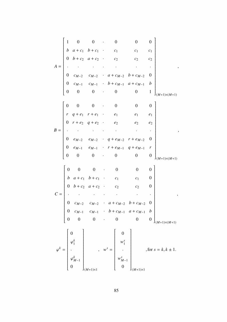
A =

1 0 0 · 0 0 0

b a + c1 b + c1 · c1 c1 c1

0 b + c2 a + c2 · c2 c2 c2

· · · · · · ·

0 cM−2 cM−2 · a + cM−2 b + cM−2 0

0 cM−1 cM−1 · b + cM−1 a + cM−1 b

0 0 0 · 0 0 1

(M+1)×(M+1)

,

B =

0 0 0 · 0 0 0

r q + e1 r + e1 · e1 e1 e1

0 r + e2 q + e2 · e2 e2 e2

· · · · · · ·

0 eM−2 eM−2 · q + eM−2 r + eM−2 0

0 eM−1 eM−1 · r + eM−1 q + eM−1 r

0 0 0 · 0 0 0

(M+1)×(M+1)

,

C =

0 0 0 · 0 0 0

b a + c1 b + c1 · c1 c1 0

0 b + c2 a + c2 · c2 c2 0

· · · · · · ·

0 cM−2 cM−2 · a + cM−2 b + cM−2 0

0 cM−1 cM−1 · b + cM−1 a + cM−1 b

0 0 0 · 0 0 0

(M+1)×(M+1)

,

ϕk =

0

ϕk1

·

ϕkM−1

0

(M+1)×1

, ws =

0

ws1

·

wsM−1

0

(M+1)×1

, for s = k, k ± 1.

85

Here,

a =1τ2 +

12h2 , b = −

14h2 , ,r = −

12h2 ,q =

1h2 −

2τ2 ,

cn =12

sin xn(cos 2h − 1)

dh, en = sin xn

(cos 2h − 1)dh

,

d =M−1∑i=1(1 + sin xi) h,1 6 n 6 M − 1,

ϕkn = 4e−2tk sin xn +

(e−2tk+1 + 2e−2tk + e−2tk−1

)(cos 2h − 1)

h2 ∑M−1i=1 (1 + sin xi) h

sin 2xn,

1 6 k 6 N − 1,1 6 n 6 M − 1.

Finally, we obtain w1.Applying the formula

w1n − w

0n

τ−τ

h2(w1

n+1 − 2w1n + w

1n−1

)+

2τ(cos 2h − 1)h2 ∑M−1

i=1 (1 + sin xi) hsin 2xn

∑M−1i=1 w1

i h

+τ

2h2

(w0

n+1 − 2w0n + w

0n−1

)= 2τ sin 2xn − 2 (1 + sin 2xn) +

2τπe−2t1(cos 2h − 1)h2 ∑M−1

i=1 (1 + sin xi) hsin 2xn,

and conditions w10 = w1

M,w11 − w

10 = w1

M − w1M−1we get

Ew1 + Fw0 = γ. (3.53)

Here

E =

1 0 0 · 0 0 0

y x + z1 y + z1 · z1 z1 0

0 y + z2 x + z2 · z2 z2 0

· · · · · · ·

0 zM−2 zM−2 · x + zM−2 y + zM−2 0

0 zM−1 zM−1 · y + zM−1 x + zM−1 y

0 0 0 · 0 0 1

(M+1)×(M+1)

,

x = −2τh2 +

1τ, y = −

τ

h2 , zn =2τ(cos 2h − 1)

dhsin 2xn,

u = −τ

2h2 , v =1τ+τ

h2 , v = −32τ−

2τh2 + 1,

86

F =

0 0 0 · 0 0 0

u v u · 0 0 0

0 u v · 0 0 0

· · · · · · ·

0 0 0 · v u 0

0 0 0 · u v u

0 0 0 · 0 0 0

(M+1)×(M+1)

,

γ =

0

∇1

·

∇M−1

0

(M+1)×1

,

∇n = 2τ sin 2xn − 2 (1 + sin 2xn) +2τπe−2t1(cos 2h − 1)h2 ∑M−1

i=1 (1 + sin xi) hsin 2xn.

From that, it follows

w1 = E−1(γ − Fw0

). (3.54)



nN

k=0

M

n=0by (3.52). Now, applying formula (3.32), we can obtain

pk =ηk+1 − 2ηk + ηk−1

τ2 ,1 ≤ k ≤ N − 1, p0 =2τ2η1 (3.55)



uknN

k=0

M

n=0by formulas (3.49) and (3.50).

The errors are computed by

Eu = max06k6N

(M−1∑n=1

u (tk, xn) − ukn

2 h

) 12

,

Ep = max16k6N−1

|p (tk) − pk | ,

87

where u (t, x) , p(t) represent the exact solution, ukn represents the numerical solutions at

(tk, xn), and pk represents the numerical solutions at tk . The numerical results are given in the

following Table.


Error N =M = 20 N =M = 40 N =M = 80 N =M = 160

Eu 0.00254 6.355e − 04 1.5675e − 04 3.9723e − 05

Ep 0.0028 7.0523e − 04 1.76857e − 04 4.4758e − 05


solution and approximate solution decreases by a factor of approximately 14 for the second-order

difference scheme (3.48).

88

CHAPTER 4

CONCLUSION

This thesis is devoted to study the source identification problem for hyperbolic differential

equations with unknown parameter p(t). The following results are obtained:

• The history of direct and inverse boundary value problems for hyperbolic differential

equations are studied.

• Fourier series, Laplace transform and Fourier transform methods are applied for the

solution of several identification problems for hyperbolic differential equations.

• The theorem on the stability estimates for the solution of the source identification

problem for hyperbolic differential equations with local and nonlocal conditions is proved.

• The first and second order of accuracy difference schemes for the approximate solution

of the one dimensional identification problem for hyperbolic differential equation with local

and nonlocal conditions are presented.

• The theorem on the stability estimates for these difference schemes for the numerical

solution of identification problems for hyperbolic differential equations with local and nonlocal

conditions is established.

• The Matlab implementation of these difference schemes is presented.

• The theoretical statements for the solution of these difference schemes are supported

by the results of numerical examples.

89

90

REFERENCES

Anikonov, Y. E. (1976). A uniqueness theorem for solution of an inverse problem for the

wave equation. Mat. Zametki, 19 (2), 211-214.

Anikonov, Y. E. (1995). Analytical representations of solutions to multidimensional

inverse problems for evolutionary equations. J. Inverse III-posed Probl, 3 (4), 259-

67.

Anikonov, Y. E. (1996). Formulas for solutions and coefficients of second-order

differential equations. Siberian Mathematical Journal, 37(3), 415-422.

Anikonov, Y. E., & Neshchadim, M. V. (2011). On analytical methods in the theory of

inverse problems for hyperbolic equations. I. Journal of Applied and Industrial

Mathematics, 5(4), 506-518.

Anikonov, Y. E., & Neshchadim, M. V. (2012 a). On analytical methods in the theory of

inverse problems for hyperbolic equations. II. Journal of Applied and Industrial

Mathematics, 6(1), 6-11.

Anikonov, Y. E., & Neshchadim, M. V. (2012 b). Representations for the solutions and

coefficients of second-order differential equations. Sibirskii Zhurnal Industrial'noi

Matematiki, 15(4), 17-23.

Ashyralyev, A. (2011). On the problem of determining the parameter of a parabolic

equation. Ukrainian Mathematical Journal, 62(9), 1397-1408.

Ashyralyev, A., & Agirseven, D. (2014). On source identification problem for a delay

parabolic equation. Nonlinear Anal., Model. Control, 19(3), 335-349.

Ashyralyev, A., & Ashyralyyev, C. (2014). On the problem of determining the parameter

of an elliptic equation in a Banach space. Nonlinear Anal. Model. Control, 19(3),

350-66.

Ashyralyev, A., & Çekiç, F. (2015, May). On source identification problem for telegraph

differential equations. In International Conference on Differential & Difference

Equations and Applications (pp. 39-50). Springer, Cham.

Ashyralyev, A., & Emharab, F. (2017). Source identification problems for hyperbolic

differential and difference equations, AIP Conference Proceedings 1880, 04000);

doi: 10.1063/1.5000617.

91

Ashyralyev, A., & Emharab, F. (2018a). Identification hyperbolic problems with nonlocal

conditions. In Proceedings of the 4th International Conference on Analysis and

Applied Mathematics Volume: 1997 Article Number: UNSP 020031-1. DOI:

10.1063/1.5049025.

Ashyralyev, A., & Emharab, F. (2018b). Second Order Difference Scheme for the

Numerical Processing of Source Identification Terms in Hyperbolic Equations. In

Proceedings of the 4th International Conference on Analysis and Applied

Mathematics Volume: 1997 Article Number: UNSP 020005-1. DOI:

10.1063/1.5048999.

Ashyralyev, A., & Emharab, F. (2018c). Identification hyperbolic problems with the

Neumann boundary condition, Bulletin of the Karaganda University-Mathematics,

3(91), 89-98.

Ashyralyev, A., & Emharab, F. (2018d). Source identification problems for hyperbolic

differential and difference equations. J. Inverse III-posed Probl, DOI:

https://doi.org/10.1515/jiip-2018-0020.

Ashyralyev, A., & Erdogan, A. (2014). Well-Posedness of the Right-Hand Side

Identification Problem for a Parabolic Equation. Ukrainian Mathematical Journal,

66(2).

Ashyralyev, A., Erdogan, A. S., & Demirdag, O. (2012). On the determination of the right-

hand side in a parabolic equation. Applied Numerical Mathematics, 62(11), 1672-

683.

Ashyralyev, A., Pastor, J., Piskarev, S., & Yurtsever, H. A. (2015). Second order equations

in functional spaces: qualitative and discrete well-posedness. In Abstract and

Applied Analysis, (Vol. 2015). Hindawi

Ashyralyev, A., & Sobolevskii, P. E. (2004). New difference schemes for partial

differential equations (Vol. 148). Birkhäuser.

Ashyralyyev, C. (2014). High order of accuracy difference schemes for the inverse elliptic

problem with Dirichlet condition. Boundary Value Problems, 2014(1), 5.

Ashyralyyev, C., & Demirdag, O. (2012). The difference problem of obtaining the

parameter of a parabolic equation. In Abstract and Applied Analysis, (Vol. 2012).

Hindawi.

92

Belov,Y. Y. (2002). Inverse problems for partial differential equations, Inverse Ill-Posed

Probl. Ser., VSP, Utrecht.

Borukhov, V. T., & Vabishchevich, P. N. (2000). Numerical solution of the inverse

problem of reconstructing a distributed right-hand side of a parabolic equation.

Computer physics communications, 126(1-2), 32-36.

Choulli, M., & Yamamoto, M. (1999). Generic well-posedness of a linear inverse parabolic

problem with diffusion parameters. Journal of Inverse and Ill-Posed Problems,

7(3), 241-254.

Dehghan, M. (2003). Finding a control parameter in one-dimensional parabolic equations.

Applied Mathematics and Computation, 135(2-3), 491-503.

Di Blasio, G., & Lorenzi, A. (2007). Identification problems for parabolic delay differential

equations with measurement on the boundary. Journal of Inverse and Ill-posed

Problems jiip, 15(7), 709-734.

Erdogan, A. S., & Sazaklioglu, A. U. (2014). A note on the numerical solution of an

identification problem for observing two-phase flow in capillaries. Mathematical

Methods in the Applied Sciences, 37(16), 2393-2405.

Èidel'man, Y. S. (1978). A boundary value problem for a differential equation with a

parameter. Differentsial'nye Uravneniya, 14(7), 1335-1337.

Gryazin, Y. A., Klibanov, M. V., & Lucas, T. R. (1999). Imaging the diffusion coefficient

in a parabolic inverse problem in optical tomography. Inverse Problems, 15(2), 373.

Isakov, V. (1998). Inverse problems for partial differential equations, Appl. Math. Sci.

127, Springer, New York.

Ivanchov, N. I. (1995). On the determination of unknown source in the heat equation with

nonlocal boundary conditions. Ukrainian Mathematical Journal, 47(10), 1647-

1652.

Kabanikhin, S. I., & Krivorotko, O. I. (2015). Identification of biological models described

by systems of nonlinear differential equations. Journal of Inverse and Ill-posed

Problems, 23(5), 519-527.

Kostin, A. B. (2013). The inverse problem of reconstructing a source in a parabolic

equation from the nonlocal observation condition. Mat. Sb, 204(10), 3-46.

93

Kozhanov, A. I. (1997). Questions of posing and solvability of linear inverse problems for

elliptic equations. Journal of Inverse and Ill-Posed Problems, 5(4), 337-352.

Kozhanov, A. I., & Safiullova, R. R. (2010). Linear inverse problems for parabolic and

hyperbolic equations. Journal of Inverse and Ill-Posed Problems, 18(1), 1-24.

Kozhanov, A. I., & Safiullova, R. R. (2017). Determination of parameters in telegraph

equation. Ufimskii Matematicheskii Zhurnal, 9(1), 63-74.

Kozhanov, A. I., & Telesheva, L. A. (2017). Nonlinear inverse problems with integral

overdetermination for nonstationary differential equations of high order. Vestnik

Yuzhno-Ural'skogo Universiteta. Seriya Matematicheskoe Modelirovanie

Programmirovanie, 10(2), 24-37.

Orlovskii, D. G. (2008). Inverse Dirichlet problem for an equation of elliptic type.

Differential Equations, 44(1), 124-134.

Orlovskii, D. G., & Piskarev, S. I. (2013). Approximation of the Bitsadze-Samarskii

inverse problem for an elliptic equation with the Dirichlet conditions. Differential

Equations, 49(7), 895-907.

Orlovskii, D. G., & Prilepko, A. I. (1987). Some inverse problems for the linearized

Boltzmann equation. USSR Computational Mathematics and Mathematical Physics,

27(6), 58-65.

Prilepko, A. I., Orlovsky, D. G., & Vasin, I. A. (2000). Methods for solving inverse

problems in mathematical physics. CRC Press.

Saitoh, S., Tuan, V. K., & Yamamoto, M. (2003). Reverse convolution inequalities and

applications to inverse heat source problems. J. Inequal. Pure Appl. Math, 3(5), 80.

Samarskii, A. A., & Vabishchevich, P. N. (2008). Numerical methods for solving inverse

problems of mathematical physics (Vol. 52). Walter de Gruyter.

Sobolevskii, P. E., & Chebotareva, L. M. (1977). Approximate solution of the Cauchy

problem for an abstract hyperbolic equation by the method of lines. Izvestiya

Vysshikh Uchebnykh Zavedenii. Matematika, (5), 103-116.

APPENDICES

95

Appendix 1

Matlab Programming

Matlab Implementation of Difference Schemes (2.69)

clc; clear all ; close all;

N=160;

M=160;

h=pi/M; tau=1/N;

a=(1/(tau^2))+(2/(h^2));

e=-2/(tau^2);

b=-1/(h^2);

g=1/(tau^2);

d=0;

for i=1:M-1;

d=d+h*sin(i*h);

end;

z=2*(cos(h)-1)/(d*h);

A=zeros(M+1,M+1);

for i=2:M;

for j=2:M;

A(i,j)=z*sin((i-1)*h);

end;

end;

for i=2:M

A(i,i)=a+(z*sin((i-1)*h));

end;

for i=2:M-1;

A(i,i+1)=b+(z*sin((i-1)*h));

end;

for i=3:M;

96

A(i,i-1)=b+(z*sin((i-1)*h));

end;

A(1,1)=1;A(M+1,M+1)=1;A(2,1)=b;A(M,M+1)=b;

A;

B=zeros(M+1,M+1);

for n=2:M;

B(n,n)=e;

end;

B;

C=zeros(M+1,M+1);

for n=2:M;

C(n,n)=g;

end;

C;

fii=zeros(M+1,1);

for j=1:M+1;

for k=2:N;

fii(j,k)=((4*(cos(h)-1)/(d*(h^2)))+1)*exp(-k*tau)*sin((j-1)*h);

end;

end;

fii;

G=inv(A);

W=zeros(M+1,1);

for j=1:M+1;

W(j,1)=sin((j-1)*h);

W(j,2)=(1-tau)*sin((j-1)*h);

for k=3:N+1;

W(:,k)=G*(-(B*W(:,k-1))-(C*W(:,k-2))+fii(:,k-1));

end;

end;

for k=2:N;

97

D=0;

for j=1:M-1;

S(j)=D+W(j,k+1)-2*(W(j,k))+W(j,k-1);

D=S(j);

end;

p(k)=(2*exp(-(k+1)*tau)-4*exp(-k*tau)+2*exp(-(k-1)*tau)-(h*D))/(d*(tau^2));

end;

p(k);

L=zeros(M+1,M+1);

for i=2:M;

for j=2:M;

L(i,j)=0;

end

end;

for i=2:M;

L(i,i)=a;

end;

for i=2:M-1;

L(i,i+1)=b;

end;

for i=3:M;

L(i,i-1)=b;

end;

L(1,1)=1;

L(M+1,M+1)=1;

L;

B=zeros(M+1,M+1);

for n=2:M;

B(n,n)=e;

end;

B;

98

C=zeros(M+1,M+1);

for n=2:M;

C(n,n)=g;

end;

C;

fii=zeros(M+1,1) ;

for j=1:M+1;

for k=2:N;

x=(j-1)*h;

fii(j,k)=exp(-k*tau)*sin(x)+(p(k)*sin(x));

end;

end;

fii;

G=inv(L);

u=zeros(M+1,1);

for j=1:M+1;

x=(j-1)*h;

u(j,1)=sin(x);

u(j,2)=(1-tau)*sin(x);

end;

for k=3:N+1;

u(:,k)=G*(-(B*u(:,k-1))-(C*u(:,k-2))+fii(:,k-1));

end;

%\%\%\%\%\%'EXACT SOLUTION OF THIS PDE' \%\%\%\%\%\%\%\%

for j=1:M+1;

for k=1:N+1;

t=(k-1)*tau;

x=(j-1)*h;

es(j,k)=(1-t)*sin(x);

eu(j,k)=exp(-t)*sin(x);

end;

99

end;

for k=2:N;

t=(k-1)*tau;

ep(k)=exp(-t);

end;

% ABSOLUTE DIFFERENCES ;

absdiff=max(max(abs(es-W)))

absdiff=max(max(abs(ep-p)))

absdiff=max(max(abs(eu-u)))

100

Appendix 2

Matlab Programming



N=20;M=20;

h=pi/M; tau=1/N;

d=0;

for j=1:M-1;

d=d+h*sin((j)*h);

end;

a=1/(tau^2)+1/(2*(h^2));q=1/(h^2)-2/(tau^2);

b=-1/(4*(h^2));r=-1/(2*(h^2));

c=(cos(h)-1)/(2*d*h);e=(cos(h)-1)/(d*h);

A=zeros(M+1,M+1);

for i=2:M;

for j=2:M;

A(i,j)=c*sin((i-1)*h);

end;

end;

for i=2:M

A(i,i)=a+c*sin((i-1)*h);

end;

for i=2:M-1;

A(i,i+1)=b+c*sin((i-1)*h);

end;

for i=3:M;

A(i,i-1)=b+c*sin((i-1)*h);

end;

A(1,1)=1;A(M+1,M+1)=1;A(2,1)=b;A(M,M+1)=b;

101

A;

B=zeros(M+1,M+1);

for i=2:M;

for j=2:M;

B(i,j)=e*sin((i-1)*h);

end;

end;

for i=2:M

B(i,i)=q+e*sin((i-1)*h);

end;

for i=2:M-1;

B(i,i+1)=r+e*sin((i-1)*h);

end;

for i=3:M;

B(i,i-1)=r+e*sin((i-1)*h);

end;

B(2,1)=r;B(M,M+1)=r;

B;

C=zeros(M+1,M+1);

for i=2:M;

for j=2:M;

C(i,j)=c*sin((i-1)*h);

end;

end;

for i=2:M

C(i,i)=a+c*sin((i-1)*h);

end;

for i=2:M-1;

C(i,i+1)=b+c*sin((i-1)*h);

end;

for i=3:M;

102

C(i,i-1)=b+c*sin((i-1)*h);

end;

C(2,1)=b;C(M,M+1)=b;

C;

fii=zeros(M+1,1);

for j=1:M+1;

for k=2:N;

fii(j,k)=exp(-(k-1)*tau)*sin((j-1)*h)+(exp(-k*tau)+2*exp(-(k-1)*tau)+exp(-(k-

2)*tau))*sin((j-1)*h)*((cos(h)-1)/(d*(h^2)));

end;

end;

e1=-tau/(h^2);e2=(2*tau)/(h^2)+1/tau;

y=(2*tau*(cos(h)-1))/(d*h);

E=zeros(M+1,M+1);

for i=2:M;

for j=2:M;

E(i,j)=y*sin((i-1)*h);

end;

end;

for i=2:M

E(i,i)=e2+y*sin((i-1)*h);

end;

for i=2:M-1;

E(i,i+1)=e1+y*sin((i-1)*h);

end;

for i=3:M;

E(i,i-1)=e1+y*sin((i-1)*h);

end;

E(1,1)=1;E(M+1,M+1)=1;E(2,1)=e1;E(M,M+1)=e1;

E;

f1=tau/(2*(h^2));f2=-tau/(h^2)-1/tau;

103

F=zeros(M+1,M+1);

for i=2:M

F(i,i)=f2;

end;

for i=2:M-1;

F(i,i+1)=f1;

end;

for i=3:M;

F(i,i-1)=f1;

end;

F(2,1)=f1;F(M,M+1)=f1;

F;

phy=zeros(M+1,1);

for j=1:M+1;

phy(j)=(tau/2-1)*sin((j-1)*h)+((2*y)/h)*(exp(-tau)*sin((j-1)*h));

end;

Z=inv(E);G=inv(A);

W=zeros(M+1,1);

for j=1:M+1;

W(j,1)=sin((j-1)*h);

end;

W(:,2)=Z*(phy-F*W(:,1));

for k=3:N+1;

W(:,k)=G*(-(B*W(:,k-1))-(C*W(:,k-2))+fii(:,k-1));

end;

for k=2:N;

D=0;

for j=1:M-1;

S(j)=D+W(j,k+1)-2*(W(j,k))+W(j,k-1);

D=S(j);

104

end;

p(k)=(2*exp(-(k)*tau)-(4*exp(-(k-1)*tau))+(2*exp(-(k-2)*tau))-(h*D))/(d*(tau^2));

end;

p(k);

R=zeros(M+1,M+1);

for i=2:M

R(i,i)=a;

end;

for i=2:M-1;

R(i,i+1)=b;

end;

for i=3:M;

R(i,i-1)=b;

end;

R(1,1)=1;R(M+1,M+1)=1;R(2,1)=b;R(M,M+1)=b;

R;

L=zeros(M+1,M+1);

for i=2:M;

for j=2:M;

L(i,j)=0;

end;

end;

for i=2:M

L(i,i)=q;

end;

for i=2:M;

L(i,i+1)=r;

end;

for i=3:M;

L(i,i-1)=r;

end;

105

L(2,1)=r;L(M,M+1);

L;

Q=zeros(M+1,M+1);

for i=2:M

Q(i,i)=a;

end;

for i=2:M-1;

Q(i,i+1)=b;

end;

for i=3:M;

Q(i,i-1)=b;

end;

Q(2,1)=b;Q(M,M+1)=b;

Q;

fii=zeros(M+1,1) ;

for j=2:M;

for k=2:N;

x=(j-1)*h;

fii(j,k)=exp(-(k-1)*tau)*sin(x)+(p(k)*sin(x));

end;

end;

G=inv(R);

u=zeros(M+1,1);

for k=3:N+1;

for j=1:M+1;

x=(j-1)*h;

u(j,1)=sin(x);

u(j,2)=(1-tau+((tau^2)/(2)))*sin((j-1)*h);

u(:,k)=G*(-(L*u(:,k-1))-(Q*u(:,k-2))+fii(:,k-1));

end;

end;

106


for j=1:M+1;

for k=1:N+1;

t=(k-1)*tau; x=(j-1)*h;



end;

end;

for k=2:N;

t=(k-1)*tau;

ep(k)=exp(-t);

end





107

Appendix 3

Matlab Programming



N=160;

M=160;

h=pi/M; tau=1/N;

d=0;

for i=1:M-1;

d=d+h*sin(i*h);

end;

a=(1/(tau^2))+(1/(h^2));b=-1/(2*(h^2));g=-2/(tau^2);c=(cos(h)-1)/(d*h);

A=zeros(M+1,M+1);

for i=2:M;

for j=2:M;

A(i,j)=c*sin((i-1)*h);

end;

end;

for i=2:M

A(i,i)=a+(c*sin((i-1)*h));

end;

for i=2:M-1;

A(i,i+1)=b+(c*sin((i-1)*h));

end;

for i=3:M;

A(i,i-1)=b+(c*sin((i-1)*h));

end;

A(1,1)=1;

A(M+1,M+1)=1;

108

A(2,1)=b;

A(M,M+1)=b;

A;

B=zeros(M+1,M+1);

for n=2:M;

B(n,n)=g;

end;

B;

C=zeros(M+1,M+1);

for i=2:M;

for j=2:M;

C(i,j)=c*sin((i-1)*h);

end;

end;

for i=2:M

C(i,i)=a+(c*sin((i-1)*h));

end;

for i=2:M-1;

C(i,i+1)=b+(c*sin((i-1)*h));

end;

for i=3:M;

C(i,i-1)=b+(c*sin((i-1)*h));

end;

C(2,1)=b;

C(M,M+1)=b;

C;

fii=zeros(M+1,1);

for j=1:M+1;

for k=2:N;

fii(j,k)=(exp(-(k-1)*tau)+((2*c)/h)*exp(-k*tau)+((2*c)/h)*exp(-(k-2)*tau))*sin((j-1)*h);

109

end;

end;

e1=-tau/(h^2);

e2=(2*tau)/(h^2)+1/tau;

y=(2*tau*(cos(h)-1))/(d*h);

E=zeros(M+1,M+1);

for i=2:M;

for j=2:M;

E(i,j)=y*sin((i-1)*h);

end;

end;

for i=2:M

E(i,i)=e2+y*sin((i-1)*h);

end;

for i=2:M-1;

E(i,i+1)=e1+y*sin((i-1)*h);

end;

for i=3:M;

E(i,i-1)=e1+y*sin((i-1)*h);

end;

E(1,1)=1;

E(M+1,M+1)=1;

E(2,1)=e1;

E(M,M+1)=e1;

E;

f1=tau/(2*(h^2));

f2=-tau/(h^2)-1/tau;

F=zeros(M+1,M+1);

for i=2:M

F(i,i)=f2;

end;

110

for i=2:M-1;

F(i,i+1)=f1;

end;

for i=3:M;

F(i,i-1)=f1;

end;

F(2,1)=f1;

F(M,M+1)=f1;

F;

phy=zeros(M+1,1);

for j=1:M+1;

phy(j)=(tau/2-1)*sin((j-1)*h)+((2*y)/h)*(exp(-tau)*sin((j-1)*h));

end;

Z=inv(E);

G=inv(A);

W=zeros(M+1,1);

for j=1:M+1;

W(j,1)=sin((j-1)*h);

end;

W(:,2)=Z*(phy-F*W(:,1));

for k=3:N+1;

W(:,k)=G*(-(B*W(:,k-1))-(C*W(:,k-2))+fii(:,k-1));

end;

for k=2:N;

D=0;

for j=1:M-1;

S(j)=D+W(j,k+1)-2*(W(j,k))+W(j,k-1);

D=S(j);

end;

p(k)=(2*exp(-(k)*tau)-(4*exp(-(k-1)*tau))+(2*exp(-(k-2)*tau))-(h*D))/(d*(tau^2));

end;

111

p(k);

R=zeros(M+1,M+1);

for i=2:M

R(i,i)=a;

end;

for i=2:M-1;

R(i,i+1)=b;

end;

for i=3:M;

R(i,i-1)=b;

end;

R(1,1)=1;

R(M+1,M+1)=1;

R(2,1)=b;

R(M,M+1)=b;

R;

B=zeros(M+1,M+1);

for n=2:M;

B(n,n)=g;

end;

B;

Q=zeros(M+1,M+1);

for i=2:M

Q(i,i)=a;

end;

for i=2:M-1;

Q(i,i+1)=b;

end;

for i=3:M;

Q(i,i-1)=b;

end;

112

Q(2,1)=b;

Q(M,M+1)=b;

Q ;

fii=zeros(M+1,1) ;

for j=2:M;

for k=2:N;

x=(j-1)*h;

fii(j,k)=exp(-(k-1)*tau)*sin(x)+(p(k)*sin(x));

end;

end;

G=inv(R);

u=zeros(M+1,1);

for k=3:N+1;

for j=1:M+1;

x=(j-1)*h;

u(j,1)=sin(x);

u(j,2)=(1-tau+((tau^2)/(2)))*sin((j-1)*h);

u(:,k)=G*(-(B*u(:,k-1))-(Q*u(:,k-2))+fii(:,k-1));

end;

end;


for j=1:M+1;

for k=1:N+1;

t=(k-1)*tau;

x=(j-1)*h;


% ep(k)=exp(-t);


end;

end;

for k=2:N;

113

t=(k-1)*tau;

ep(k)=exp(-t);

end





114

Appendix 4

Matlab Programming


N=160;M=160;

h=pi/M; tau=1/N;

a=(1/(tau^2))+(2/(h^2));e=-2/(tau^2);b=-1/(h^2);g=1/(tau^2);

r=0;

for i=1:M-1;

r=r+h*(1+sin(2*(i)*h));

end;

r;

z=2*(cos(2*h)-1)/(r*(h));

A=zeros(M+1,M+1);

for i=2:M;

for j=2:M;

A(i,j)=z*sin(2*(i-1)*h);

end;

end;

for i=2:M;

A(i,i)=a+(z*sin(2*(i-1)*h));

end;

for i=2:M-1;

A(i,i+1)=b+(z*sin(2*(i-1)*h));

end;

for i=3:M;

A(i,i-1)=b+(z*sin(2*(i-1)*h));

end;

A(1,1)=1; A(M+1,M+1)=-1; A(1,M+1)=-1; A(M+1,1)=-1; A(M+1,M)=1; A(M+1,2)=1;

A(2,1)=b; A(M,M+1)=b;A;

115

B=zeros(M+1,M+1);

for n=2:M;

B(n,n)=e;

end;

B;

C=zeros(M+1,M+1);

for n=2:M;

C(n,n)=g;

end;

C;

fii=zeros(M+1,1) ;

for j=2:M;

for k=2:N;

t=(k)*tau; x=(j-1)*h;

fii(j,k)=((2*(pi)*(cos(2*h)-1)/(r*(h^2)))+4)*exp(-2*(k)*tau)*sin(2*(j-1)*h);

end;

end;

fii;

G=inv(A);

W=zeros(M+1,1);

forj=1:M+1;

x=(j-1)*h;

W(j,1)=1+sin(2*(j-1)*h);

W(j,2)=(1-2*tau)*(1+sin(2*(j-1)*h));

for k=3:N+1;

W(:,k)=G*(-(B*W(:,k-1))-(C*W(:,k-2))+fii(:,k-1));

end;

end;

D=0;

for k=2:N;

for j=1:M-1;

116

S(j)=D+(W(j,k+1)-2*(W(j,k))+W(j,k-1));

D=S(j);

end;

p(k)=(pi)*(exp(-2*(k-1)*tau))*(1/r)-((h*D)/(4*r)*(tau^2));

end;

p(k);

L=zeros(M+1,M+1);

for i=2:M;

L(i,i)=a;

end;

for i=2:M;

L(i,i+1)=b;

end;

for i=2:M;

L(i,i-1)=b;

end;

L(1,1)=1; L(M+1,M+1)=-1; L(1,M+1)=-1;L(M+1,1)=-1; L(M+1,M)=1; L(M+1,2)=1;

L;

B=zeros(M+1,M+1);

for n=2:M;

B(n,n)=e;

end;

B;

C=zeros(M+1,M+1);

for n=2:M;

C(n,n)=g;

end;

C;

fii=zeros(M+1,M+1) ;

for j=2:M;

for k=2:N;

117

x=(j-1)*h; t=(k)*tau;

fii(j,k)=4*exp(-2*t)*sin(2*(j-1)*h)+p(k)*(4+4*sin(2*(j-1)*h));

end;

end;

fii;

G=inv(L);

u=zeros(M+1,1);

for j=1:M+1;

x=(j-1)*h;

u(j,1)=(1+sin(2*(j-1)*h));

u(j,2)=(1-2*tau)*(1+sin(2*(j-1)*h));

for k=3:N+1;

u(:,k)=G*(-(B*u(:,k-1))-(C*u(:,k-2))+fii(:,k-1));

end;

end;


for j=1:M+1;

for k=1:N+1;

t=(k-1)*tau; x=(j-1)*h;

es(j,k)=(-2*t+1)*(1+sin(2*(j-1)*h));

eu(j,k)=exp(-2*t)*(1+sin(2*(j-1)*h));

end;

end;

for k=2:N;

t=(k-1)*tau;

ep(k)=exp(-2*t);

end;





118

Appendix 5

Matlab Programming



N=80;M=80;

h=pi/M; tau=1/N;

d=0;

for i=1:M;

d=d+h*(1+sin(2*(i-1)*h));

end;

a=(1/(tau^2))+(1/(2*(h^2)));

b=-1/(4*(h^2));

q=(1/(h^2))-(2/(tau^2));

r=-1/(2*(h^2));

e=(cos(2*h)-1)/(d*h);

c=(cos(2*h)-1)/(2*d*h);

A=zeros(M+1,M+1);

for i=2:M;

for j=2:M;

A(i,j)=c*sin(2*(i-1)*h);

end;

end;

for i=2:M

A(i,i)=a+c*sin(2*(i-1)*h);

end;

for i=2:M-1;

A(i,i+1)=b+c*sin(2*(i-1)*h);

end;

for i=3:M;

119

A(i,i-1)=b+c*sin(2*(i-1)*h);

end;

A(1,1)=1; A(1,M+1)=-1; A(2,1)=b; A(M,M+1)=b;

A(M+1,1)=-3; A(M+1,2)=4; A(M+1,3)=-1;

A(M+1,M-1)=-1;A(M+1,M)=4;A(M+1,M+1)=-3;

B=zeros(M+1,M+1);

for i=2:M;

for j=2:M;

B(i,j)=e*sin(2*(i-1)*h);

end;

end;

for i=2:M

B(i,i)=q+(e*sin(2*(i-1)*h));

end;

for i=2:M-1;

B(i,i+1)=r+(e*sin(2*(i-1)*h));

end;

for i=3:M;

B(i,i-1)=r+(e*sin(2*(i-1)*h));

end;

B(2,1)=r;B(M,M+1)=r;

B;

C=zeros(M+1,M+1);

for i=2:M;

for j=2:M;

C(i,j)=c*sin(2*(i-1)*h);

end;

end;

for i=2:M

C(i,i)=a+(c*sin(2*(i-1)*h));

end;

120

for i=2:M-1;

C(i,i+1)=b+(c*sin(2*(i-1)*h));

end;

for i=3:M;

C(i,i-1)=b+(c*sin(2*(i-1)*h));

end;

C(2,1)=b;C(M,M+1)=b;

fii=zeros(M+1,1);

for j=2:M;

for k=1:N+1;

fii(j,k)=(4*exp(-2*(k-1)*tau))*sin(2*(j-1)*h)

+((c*(pi))/h)*(exp(-2*(k)*tau)+2*exp(-2*(k-1)*tau)+exp(-2*(k-2)*tau))*sin(2*(j-1)*h);

end;

end;

ee1=-tau/(h^2);

ee2=(2*tau)/(h^2)+1/tau;

y=((2*tau)*(cos(2*h)-1))/(d*h);

E=zeros(M+1,M+1);

for i=2:M;

for j=2:M;

E(i,j)=y*sin(2*(i-1)*h);

end;

end;

for i=2:M

E(i,i)=ee2+y*sin(2*(i-1)*h);

end;

for i=2:M-1;

E(i,i+1)=ee1+y*sin(2*(i-1)*h);

end;

for i=3:M;

E(i,i-1)=ee1+y*sin(2*(i-1)*h);

121

end;

E(1,1)=1; E(1,M+1)=-1; E(2,1)=ee1; E(M,M+1)=ee2;

E(M+1,1)=-3; E(M+1,2)=4;E(M+1,3)=-1;

E(M+1,M-1)=-1;E(M+1,M)=4;E(M+1,M+1)=-3;

f1=tau/(2*(h^2));f2=-tau/(h^2)-1/tau;

F=zeros(M+1,M+1);

for i=2:M

F(i,i)=f2;

end;

for i=2:M-1;

F(i,i+1)=f1;

end;

for i=3:M;

F(i,i-1)=f1;

end;

F(2,1)=f1;

F(M,M+1)=f1

phy=zeros(M+1,1);

for j=1:M+1;

phy(j)=-2*(1+sin(2*(j-1)*h))+(2*tau)*sin(2*(j-1)*h)+((y*pi)/h)*(exp(-2*tau))*sin(2*(j-

1)*h);

end;

Z=inv(E);

G=inv(A);

W=zeros(M+1,1);

for j=1:M+1;

W(j,1)=1+sin(2*(j-1)*h);

end;

W(:,2)=Z*(phy-F*W(:,1));

for k=3:N+1;

W(:,k)=G*(-(B*W(:,k-1))-(C*W(:,k-2))+fii(:,k-1));

122

end;

for k=2:N;

D=0;

for j=1:M-1;

S(j)=D+W(j,k+1)-2*(W(j,k))+W(j,k-1);

D=S(j);

end;

p(k)=((pi)*(exp(-(k)*tau)-2*exp(-(k-1)*tau)+exp(-(k-2)*tau))-(h*D))/(4*d*(tau^2));

end;

p(k);

R=zeros(M+1,M+1);

for i=2:M

R(i,i)=a;

end;

for i=2:M-1;

R(i,i+1)=b;

end;

for i=3:M;

R(i,i-1)=b;

end;

R(1,1)=1;

R(M+1,M+1)=1;

R(2,1)=b;

R(M,M+1)=b;

R;

L=zeros(M+1,M+1);

for i=2:M;

for j=2:M;

L(i,j)=0;

end;

end;

123

for i=2:M

L(i,i)=q;

end;

for i=2:M;

L(i,i+1)=r;

end;

for i=3:M;

L(i,i-1)=r;

end;

L(2,1)=r;

L(M,M+1);

L;

Q=zeros(M+1,M+1);

for i=2:M

Q(i,i)=a;

end;

for i=2:M-1;

Q(i,i+1)=b;

end;

for i=3:M;

Q(i,i-1)=b;

end;

Q(2,1)=b;

Q(M,M+1)=b;

Q ;

fii=zeros(M+1,M+1) ;

for j=2:M;

for k=2:N;

x=(j-1)*h;

t=(k)*tau;

fii(j,k)=4*exp(-2*t)*sin(2*(j-1)*h)+4*p(k)*(1+sin(2*(j-1)*h));

124

end;

end;

fii;

G=inv(R);

u=zeros(M+1,1);

for k=3:N+1;

for j=1:M+1;

x=(j-1)*h;

u(j,1)=1+sin(2*(j-1)*h);

u(j,2)=(1-2*tau+2*(tau^2))*(1+sin(2*(j-1)*h));

u(:,k)=G*(-(L*u(:,k-1))-(Q*u(:,k-2))+fii(:,k-1));

end;

end;


for j=1:M+1;

for k=1:N+1;

t=(k-1)*tau;

x=(j-1)*h;

es(j,k)=(-2*t+1)*(1+sin(2*(j-1)*h));

eu(j,k)=exp(-2*t)*(1+sin(2*(j-1)*h));

end;

end;

for k=2:N;

t=(k-1)*tau;

ep(k)=exp(-2*t);

end;





SOURCE IDENTIFICATION PROBLEMS FOR HYPERBOLIC...

Documents

Transcript of SOURCE IDENTIFICATION PROBLEMS FOR HYPERBOLIC...