Source Coding: Part I of Fundamentals of Source and Video...
224
Foundations and Trends R in sample Vol. 1, No 1 (2011) 1–217 c 2011 Thomas Wiegand and Heiko Schwarz DOI: xxxxxx Source Coding: Part I of Fundamentals of Source and Video Coding Thomas Wiegand 1 and Heiko Schwarz 2 1 Berlin Institute of Technology and Fraunhofer Institutefor Telecommunica- tions — Heinrich Hertz Institute, Germany, [email protected] 2 Fraunhofer Institute for Telecommunications — Heinrich Hertz Institute, Germany, [email protected] Abstract Digital media technologies have become an integral part of the way we create, communicate, and consume information. At the core of these technologies are source coding methods that are described in this text. Based on the fundamentals of information and rate distortion theory, the most relevant techniques used in source coding algorithms are de- scribed: entropy coding, quantization as well as predictive and trans- form coding. The emphasis is put onto algorithms that are also used in video coding, which will be described in the other text of this two-part monograph.
Transcript of Source Coding: Part I of Fundamentals of Source and Video...

Foundations and TrendsR© insampleVol. 1, No 1 (2011) 1–217c© 2011 Thomas Wiegand and Heiko SchwarzDOI: xxxxxx
Source Coding:
Part I of Fundamentals of Sourceand Video Coding
Thomas Wiegand1 and Heiko Schwarz2
1 Berlin Institute of Technology and Fraunhofer Institute for Telecommunica-
tions — Heinrich Hertz Institute, Germany, [email protected] Fraunhofer Institute for Telecommunications — Heinrich Hertz Institute,
Germany, [email protected]
Abstract
Digital media technologies have become an integral part of the way we
create, communicate, and consume information. At the core of these
technologies are source coding methods that are described in this text.
Based on the fundamentals of information and rate distortion theory,
the most relevant techniques used in source coding algorithms are de-
scribed: entropy coding, quantization as well as predictive and trans-
form coding. The emphasis is put onto algorithms that are also used in
video coding, which will be described in the other text of this two-part
monograph.

To our families


Contents
1 Introduction 1
1.1 The Communication Problem 3
1.2 Scope and Overview of the Text 4
1.3 The Source Coding Principle 5
2 Random Processes 7
2.1 Probability 8
2.2 Random Variables 9
2.2.1 Continuous Random Variables 10
2.2.2 Discrete Random Variables 11
2.2.3 Expectation 13
2.3 Random Processes 14
2.3.1 Markov Processes 16
2.3.2 Gaussian Processes 18
2.3.3 Gauss-Markov Processes 18
2.4 Summary of Random Processes 19
i

ii Contents
3 Lossless Source Coding 20
3.1 Classification of Lossless Source Codes 21
3.2 Variable-Length Coding for Scalars 22
3.2.1 Unique Decodability 22
3.2.2 Entropy 27
3.2.3 The Huffman Algorithm 29
3.2.4 Conditional Huffman Codes 31
3.2.5 Adaptive Huffman Codes 33
3.3 Variable-Length Coding for Vectors 33
3.3.1 Huffman Codes for Fixed-Length Vectors 34
3.3.2 Huffman Codes for Variable-Length Vectors 36
3.4 Elias Coding and Arithmetic Coding 40
3.4.1 Elias Coding 41
3.4.2 Arithmetic Coding 47
3.5 Probability Interval Partitioning Entropy Coding 52
3.6 Comparison of Lossless Coding Techniques 61
3.7 Adaptive Coding 62
3.8 Summary of Lossless Source Coding 64
4 Rate Distortion Theory 66
4.1 The Operational Rate Distortion Function 67
4.1.1 Distortion 68
4.1.2 Rate 70
4.1.3 Operational Rate Distortion Function 70
4.2 The Information Rate Distortion Function 72
4.2.1 Mutual Information 72
4.2.2 Information Rate Distortion Function 76
4.2.3 Properties of the Rate Distortion Function 80
4.3 The Shannon Lower Bound 81
4.3.1 Differential Entropy 81
4.3.2 Shannon Lower Bound 85
4.4 Rate Distortion Function for Gaussian Sources 89
4.4.1 Gaussian IID Sources 90
4.4.2 Gaussian Sources with Memory 91

Contents iii
4.5 Summary of Rate Distortion Theory 98
5 Quantization 100
5.1 Structure and Performance of Quantizers 101
5.2 Scalar Quantization 104
5.2.1 Scalar Quantization with Fixed-Length Codes 106
5.2.2 Scalar Quantization with Variable-Length Codes 111
5.2.3 High-Rate Operational Distortion Rate Functions 119
5.2.4 Approximation for Distortion Rate Functions 125
5.2.5 Performance Comparison for Gaussian Sources 127
5.2.6 Scalar Quantization for Sources with Memory 129
5.3 Vector Quantization 133
5.3.1 Vector Quantization with Fixed-Length Codes 133
5.3.2 Vector Quantization with Variable-Length Codes 137
5.3.3 The Vector Quantization Advantage 138
5.3.4 Performance and Complexity 142
5.4 Summary of Quantization 144
6 Predictive Coding 146
6.1 Prediction 148
6.2 Linear Prediction 152
6.3 Optimal Linear Prediction 154
6.3.1 One-Step Prediction 156
6.3.2 One-Step Prediction for Autoregressive Processes 158
6.3.3 Prediction Gain 160
6.3.4 Asymptotic Prediction Gain 160
6.4 Differential Pulse Code Modulation (DPCM) 163
6.4.1 Linear Prediction for DPCM 165
6.4.2 Adaptive Differential Pulse Code Modulation 172
6.5 Summary of Predictive Coding 174
7 Transform Coding 176
7.1 Structure of Transform Coding Systems 179
7.2 Orthogonal Block Transforms 180

iv Contents
7.3 Bit Allocation for Transform Coefficients 187
7.3.1 Approximation for Gaussian Sources 188
7.3.2 High-Rate Approximation 190
7.4 The Karhunen Loeve Transform (KLT) 191
7.4.1 On the Optimality of the KLT 193
7.4.2 Asymptotic Operational Distortion Rate Function 197
7.4.3 Performance for Gauss-Markov Sources 199
7.5 Signal-Independent Unitary Transforms 200
7.5.1 The Walsh-Hadamard Transform (WHT) 201
7.5.2 The Discrete Fourier Transform (DFT) 201
7.5.3 The Discrete Cosine Transform (DCT) 203
7.6 Transform Coding Example 205
7.7 Summary of Transform Coding 207
8 Summary 209
Acknowledgements 212
References 213

1
Introduction
The advances in source coding technology along with the rapid develop-
ments and improvements of network infrastructures, storage capacity,
and computing power are enabling an increasing number of multime-
dia applications. In this text, we will describe and analyze fundamental
source coding techniques that are found in a variety of multimedia ap-
plications, with the emphasis on algorithms that are used in video cod-
ing applications. The present first part of the text concentrates on the
description of fundamental source coding techniques, while the second
part describes their application in modern video coding.
The application areas of digital video today range from multi-
media messaging, video telephony, and video conferencing over mo-
bile TV, wireless and wired Internet video streaming, standard- and
high-definition TV broadcasting, subscription and pay-per-view ser-
vices to personal video recorders, digital camcorders, and optical stor-
age media such as the digital versatile disc (DVD) and Blu-Ray disc.
Digital video transmission over satellite, cable, and terrestrial channels
is typically based on H.222.0/MPEG-2 systems [37], while wired and
wireless real-time conversational services often use H.32x [32, 33, 34] or
SIP [64], and mobile transmission systems using the Internet and mo-
1

2 Introduction
bile networks are usually based on RTP/IP [68]. In all these application
areas, the same basic principles of video compression are employed.
EncoderChannel Modu-
lator
DecoderDemodu-Channel
Capture
lator
Video
Human
SceneVideo
Encoder
Error Control ChannelVideoCodec
b
b’s’
s
VideoDecoder
Channel
VideoDisplayObserver
Fig. 1.1 Typical structure of a video transmission system.
The block structure for a typical video transmission scenario is il-
lustrated in Fig. 1.1. The video capture generates a video signal s that
is discrete in space and time. Usually, the video capture consists of a
camera that projects the 3-dimensional scene onto an image sensor.
Cameras typically generate 25 to 60 frames per second. For the con-
siderations in this text, we assume that the video signal s consists of
progressively-scanned pictures. The video encoder maps the video sig-
nal s into the bitstream b. The bitstream is transmitted over the error
control channel and the received bitstream b′ is processed by the video
decoder that reconstructs the decoded video signal s′ and presents it
via the video display to the human observer. The visual quality of the
decoded video signal s′ as shown on the video display affects the view-
ing experience of the human observer. This text focuses on the video
encoder and decoder part, which is together called a video codec.
The error characteristic of the digital channel can be controlled by
the channel encoder, which adds redundancy to the bits at the video
encoder output b. The modulator maps the channel encoder output
to an analog signal, which is suitable for transmission over a phys-
ical channel. The demodulator interprets the received analog signal
as a digital signal, which is fed into the channel decoder. The chan-
nel decoder processes the digital signal and produces the received bit-
stream b′, which may be identical to b even in the presence of channel
noise. The sequence of the five components, channel encoder, modula-

1.1. The Communication Problem 3
tor, channel, demodulator, and channel decoder, are lumped into one
box, which is called the error control channel. According to Shannon’s
basic work [69, 70] that also laid the ground to the subject of this text,
by introducing redundancy at the channel encoder and by introducing
delay, the amount of transmission errors can be controlled.
1.1 The Communication Problem
The basic communication problem may be posed as conveying source
data with the highest fidelity possible without exceeding an available
bit rate, or it may be posed as conveying the source data using the
lowest bit rate possible while maintaining a specified reproduction fi-
delity [69]. In either case, a fundamental trade-off is made between bit
rate and signal fidelity. The ability of a source coding system to suit-
able choose this trade-off is referred to as its coding efficiency or rate
distortion performance. Video codecs are thus primarily characterized
in terms of:
• throughput of the channel: a characteristic influenced by the
transmission channel bit rate and the amount of protocol
and error-correction coding overhead incurred by the trans-
mission system;
• distortion of the decoded video: primarily induced by the
video codec and by channel errors introduced in the path
to the video decoder.
However, in practical video transmission systems, the following addi-
tional issues must be considered:
• delay: a characteristic specifying the start-up latency and
end-to-end delay. The delay is influenced by many parame-
ters, including the processing and buffering delay, structural
delays of video and channel codecs, and the speed at which
data are conveyed through the transmission channel;
• complexity: a characteristic specifying the computational
complexity, the memory capacity, and memory access re-
quirements. It includes the complexity of the video codec,
protocol stacks, and network.

4 Introduction
The practical source coding design problem can be stated as follows:
Given a maximum allowed delay and a maximum al-
lowed complexity, achieve an optimal trade-off between
bit rate and distortion for the range of network environ-
ments envisioned in the scope of the applications.
1.2 Scope and Overview of the Text
This text provides a description of the fundamentals of source and video
coding. It is aimed at aiding students and engineers to investigate the
subject. When we felt that a result is of fundamental importance to the
video codec design problem, we chose to deal with it in greater depth.
However, we make no attempt to exhaustive coverage of the subject,
since it is too broad and too deep to fit the compact presentation
format that is chosen here (and our time limit to write this text).
We will also not be able to cover all the possible applications of video
coding. Instead our focus is on the source coding fundamentals of video
coding. This means that we will leave out a number of areas including
implementation aspects of video coding and the whole subject of video
transmission and error-robust coding.
The text is divided into two parts. In the first part, the fundamentals
of source coding are introduced, while the second part explains their
application to modern video coding.
Source Coding Fundamentals. In the present first part, we de-
scribe basic source coding techniques that are also found in video
codecs. In order to keep the presentation simple, we focus on the de-
scription for 1-d discrete-time signals. The extension of source coding
techniques to 2-d signals, such as video pictures, will be highlighted in
the second part of the text in the context of video coding. Chapter 2
gives a brief overview of the concepts of probability, random variables,
and random processes, which build the basis for the descriptions in
the following chapters. In Chapter 3, we explain the fundamentals of
lossless source coding and present lossless techniques that are found
in the video coding area in some detail. The following chapters deal
with the topic of lossy compression. Chapter 4 summarizes important

1.3. The Source Coding Principle 5
results of rate distortion theory, which builds the mathematical basis
for analyzing the performance of lossy coding techniques. Chapter 5
treats the important subject of quantization, which can be consid-
ered as the basic tool for choosing a trade-off between transmission
bit rate and signal fidelity. Due to its importance in video coding, we
will mainly concentrate on the description of scalar quantization. But
we also briefly introduce vector quantization in order to show the struc-
tural limitations of scalar quantization and motivate the later discussed
techniques of predictive coding and transform coding. Chapter 6 cov-
ers the subject of prediction and predictive coding. These concepts are
found in several components of video codecs. Well-known examples are
the motion-compensated prediction using previously coded pictures,
the intra prediction using already coded samples inside a picture, and
the prediction of motion parameters. In Chapter 7, we explain the
technique of transform coding, which is used in most video codecs for
efficiently representing prediction error signals.
Application to Video Coding. The second part of the text will
describe the application of the fundamental source coding techniques
to video coding. We will discuss the basic structure and the basic con-
cepts that are used in video coding and highlight their application
in modern video coding standards. Additionally, we will consider ad-
vanced encoder optimization techniques that are relevant for achieving
a high coding efficiency. The effectiveness of various design aspects will
be demonstrated based on experimental results.
1.3 The Source Coding Principle
The present first part of the text describes the fundamental concepts of
source coding. We explain various known source coding principles and
demonstrate their efficiency based on 1-d model sources. For additional
information on information theoretical aspects of source coding the
reader is referred to the excellent monographs in [11, 22, 4]. For the
overall subject of source coding including algorithmic design questions,
we recommend the two fundamental texts by Gersho and Gray [16]
and Jayant and Noll [44].

6 Introduction
The primary task of a source codec is to represent a signal with the
minimum number of (binary) symbols without exceeding an “accept-
able level of distortion”, which is determined by the application. Two
types of source coding techniques are typically named:
• Lossless coding: describes coding algorithms that allow the
exact reconstruction of the original source data from the com-
pressed data. Lossless coding can provide a reduction in bit
rate compared to the original data, when the original signal
contains dependencies or statistical properties that can be
exploited for data compaction. It is also referred to as noise-
less coding or entropy coding. Lossless coding can only be
employed for discrete-amplitude and discrete-time signals. A
well-known use for this type of compression for picture and
video signals is JPEG-LS [40].
• Lossy coding: describes coding algorithms that are charac-
terized by an irreversible loss of information. Only an ap-
proximation of the original source data can be reconstructed
from the compressed data. Lossy coding is the primary cod-
ing type for the compression of speech, audio, picture, and
video signals, where an exact reconstruction of the source
data is not required. The practically relevant bit rate reduc-
tion that can be achieved with lossy source coding techniques
is typically more than an order of magnitude larger than that
for lossless source coding techniques. Well known examples
for the application of lossy coding techniques are JPEG [38]
for still picture coding, and H.262/MPEG-2 Video [39] and
H.264/AVC [36] for video coding.
Chapter 2 briefly reviews the concepts of probability, random vari-
ables, and random processes. Lossless source coding will be described
in Chapter 3. The Chapters 5, 6, and 7 give an introduction to the lossy
coding techniques that are found in modern video coding applications.
In Chapter 4, we provide some important results of rate distortion the-
ory, which will be used for discussing the efficiency of the presented
lossy coding techniques.

2
Random Processes
The primary goal of video communication, and signal transmission in
general, is the transmission of new information to a receiver. Since the
receiver does not know the transmitted signal in advance, the source of
information can be modeled as a random process. This permits the de-
scription of source coding and communication systems using the mathe-
matical framework of the theory of probability and random processes. If
reasonable assumptions are made with respect to the source of informa-
tion, the performance of source coding algorithms can be characterized
based on probabilistic averages. The modeling of information sources
as random processes builds the basis for the mathematical theory of
source coding and communication.
In this chapter, we give a brief overview of the concepts of proba-
bility, random variables, and random processes and introduce models
for random processes, which will be used in the following chapters for
evaluating the efficiency of the described source coding algorithms. For
further information on the theory of probability, random variables, and
random processes, the interested reader is referred to [45, 60, 25].
7

8 Random Processes
2.1 Probability
Probability theory is a branch of mathematics, which concerns the de-
scription and modeling of random events. The basis for modern prob-
ability theory is the axiomatic definition of probability that was intro-
duced by Kolmogorov in [45] using concepts from set theory.
We consider an experiment with an uncertain outcome, which is
called a random experiment. The union of all possible outcomes ζ of
the random experiment is referred to as the certain event or sample
space of the random experiment and is denoted by O. A subset A of
the sample space O is called an event. To each event A a measure P (A)
is assigned, which is referred to as the probability of the event A. The
measure of probability satisfies the following three axioms:
• Probabilities are non-negative real numbers,
P (A) ≥ 0, ∀A ⊆ O. (2.1)
• The probability of the certain event O is equal to 1,
P (O) = 1. (2.2)
• The probability of the union of any countable set of pairwise
disjoint events is the sum of the probabilities of the individual
events; that is, if {Ai : i = 0, 1, · · · } is a countable set of
events such that Ai ∩ Aj = ∅ for i 6= j, then
P
(⋃
i
Ai
)
=∑
i
P (Ai). (2.3)
In addition to the axioms, the notion of the independence of two events
and the conditional probability are introduced:
• Two events Ai and Aj are independent if the probability of
their intersection is the product of their probabilities,
P (Ai ∩ Aj) = P (Ai)P (Aj). (2.4)
• The conditional probability of an event Ai given another
event Aj, with P (Aj) > 0, is denoted by P (Ai|Aj) and is
defined as
P (Ai|Aj) =P (Ai ∩ Aj)
P (Aj). (2.5)

2.2. Random Variables 9
The definitions (2.4) and (2.5) imply that, if two events Ai and Aj are
independent and P (Aj) > 0, the conditional probability of the event Ai
given the event Aj is equal to the marginal probability of Ai,
P (Ai | Aj) = P (Ai). (2.6)
A direct consequence of the definition of conditional probability in (2.5)
is Bayes’ theorem,
P (Ai|Aj) = P (Aj |Ai)P (Ai)
P (Aj), with P (Ai), P (Aj) > 0, (2.7)
which described the interdependency of the conditional probabilities
P (Ai|Aj) and P (Aj|Ai) for two events Ai and Aj .
2.2 Random Variables
A concept that we will use throughout this text are random variables,
which will be denoted with upper-case letters. A random variable S is
a function of the sample space O that assigns a real value S(ζ) to each
outcome ζ∈ O of a random experiment.
The cumulative distribution function (cdf) of a random variable S
is denoted by FS(s) and specifies the probability of the event {S ≤ s},
FS(s) = P (S≤ s) = P ( {ζ : S(ζ)≤ s} ). (2.8)
The cdf is a non-decreasing function with FS(−∞) = 0 and FS(∞) = 1.
The concept of defining a cdf can be extended to sets of two or more
random variables S = {S0, · · · , SN−1}. The function
FS(s) = P (S≤ s) = P (S0≤ s0, · · · , SN−1≤ sN−1) (2.9)
is referred to as N -dimensional cdf, joint cdf, or joint distribution. A
set S of random variables is also referred to as a random vector and is
also denoted using the vector notation S = (S0, · · · , SN−1)T . For the
joint cdf of two random variables X and Y we will use the notation
FXY (x, y) = P (X≤ x, Y ≤ y). The joint cdf of two random vectors X
and Y will be denoted by FXY (x,y) = P (X≤ x,Y ≤ y).
The conditional cdf or conditional distribution of a random vari-
able S given an event B, with P (B)> 0, is defined as the conditional

10 Random Processes
probability of the event {S≤ s} given the event B,
FS|B(s | B) = P (S≤ s | B) =P ({S≤ s} ∩ B)
P (B). (2.10)
The conditional distribution of a random variable X given another
random variable Y is denoted by FX|Y (x|y) and defined as
FX|Y (x|y) =FXY (x, y)
FY (y)=
P (X≤ x, Y ≤ y)
P (Y ≤ y). (2.11)
Similarly, the conditional cdf of a random vector X given another ran-
dom vector Y is given by FX|Y (x|y) = FXY (x,y)/FY (y).
2.2.1 Continuous Random Variables
A random variable S is called a continuous random variable, if its cdf
FS(s) is a continuous function. The probability P (S = s) is equal to
zero for all values of s. An important function of continuous random
variables is the probability density function (pdf), which is defined as
the derivative of the cdf,
fS(s) =dFS(s)
ds⇔ FS(s) =
∫ s
−∞fS(t) dt. (2.12)
Since the cdf FS(s) is a monotonically non-decreasing function, the
pdf fS(s) is greater than or equal to zero for all values of s. Important
examples for pdf’s, which we will use later in this text, are given below.
Uniform pdf:
fS(s) = 1/A for −A/2 ≤ s ≤ A/2, A > 0 (2.13)
Laplacian pdf:
fS(s) =1
σS
√2
e−|s−µS |√
2/σS , σS > 0 (2.14)
Gaussian pdf:
fS(s) =1
σS
√2π
e−(s−µS)2/(2σ2S ), σS > 0 (2.15)

2.2. Random Variables 11
The concept of defining a probability density function is also extended
to random vectors S = (S0, · · · , SN−1)T . The multivariate derivative
of the joint cdf FS(s),
fS(s) =∂NFS(s)
∂s0 · · · ∂sN−1, (2.16)
is referred to as the N -dimensional pdf, joint pdf, or joint density. For
two random variables X and Y , we will use the notation fXY (x, y) for
denoting the joint pdf of X and Y . The joint density of two random
vectors X and Y will be denoted by fXY (x,y).
The conditional pdf or conditional density fS|B(s|B) of a random
variable S given an event B, with P (B) > 0, is defined as the derivative
of the conditional distribution FS|B(s|B), fS|B(s|B) = dFS|B(s|B)/ds.
The conditional density of a random variable X given another random
variable Y is denoted by fX|Y (x|y) and defined as
fX|Y (x|y) =fXY (x, y)
fY (y). (2.17)
Similarly, the conditional pdf of a random vector X given another
random vector Y is given by fX|Y (x|y) = fXY (x,y)/fY (y).
2.2.2 Discrete Random Variables
A random variable S is said to be a discrete random variable if its
cdf FS(s) represents a staircase function. A discrete random variable S
can only take values of a countable set A = {a0, a1, . . .}, which is called
the alphabet of the random variable. For a discrete random variable S
with an alphabet A, the function
pS(a) = P (S = a) = P ( {ζ : S(ζ)= a} ), (2.18)
which gives the probabilities that S is equal to a particular alphabet
letter, is referred to as probability mass function (pmf). The cdf FS(s)
of a discrete random variable S is given by the sum of the probability
masses p(a) with a≤ s,
FS(s) =∑
a≤s
p(a). (2.19)

12 Random Processes
With the Dirac delta function δ it is also possible to use a pdf fS for
describing the statistical properties of a discrete random variables S
with a pmf pS(a),
fS(s) =∑
a∈Aδ(s − a) pS(a). (2.20)
Examples for pmf’s that will be used in this text are listed below. The
pmf’s are specified in terms of parameters p and M , where p is a real
number in the open interval (0, 1) and M is an integer greater than 1.
The binary and uniform pmf are specified for discrete random variables
with a finite alphabet, while the geometric pmf is specified for random
variables with a countably infinite alphabet.
Binary pmf:
A = {a0, a1}, pS(a0) = p, pS(a1) = 1− p (2.21)
Uniform pmf:
A = {a0, a1, · · ·, aM−1}, pS(ai) = 1/M, ∀ ai ∈ A (2.22)
Geometric pmf:
A = {a0, a1, · · · }, pS(ai) = (1− p) pi, ∀ ai ∈ A (2.23)
The pmf for a random vector S = (S0, · · · , SN−1)T is defined by
pS(a) = P (S = a) = P (S0 = a0, · · · , SN−1 = aN−1) (2.24)
and is also referred to as N -dimensional pmf or joint pmf. The joint
pmf for two random variables X and Y or two random vectors X and Y
will be denoted by pXY (ax, ay) or pXY (ax,ay), respectively.
The conditional pmf pS|B(a | B) of a random variable S given an
event B, with P (B) > 0, specifies the conditional probabilities of the
events {S = a} given the event B, pS|B(a | B) = P (S = a | B). The con-
ditional pmf of a random variable X given another random variable Y
is denoted by pX|Y (ax|ay) and defined as
pX|Y (ax|ay) =pXY (ax, ay)
pY (ay). (2.25)
Similarly, the conditional pmf of a random vector X given another
random vector Y is given by pX|Y (ax|ay) = pXY (ax,ay)/pY (ay).

2.2. Random Variables 13
2.2.3 Expectation
Statistical properties of random variables are often expressed using
probabilistic averages, which are referred to as expectation values or
expected values. The expectation value of an arbitrary function g(S) of
a continuous random variable S is defined by the integral
E{g(S)} =
∫ ∞
−∞g(s) fS(s) ds. (2.26)
For discrete random variables S, it is defined as the sum
E{g(S)} =∑
a∈Ag(a) pS(a). (2.27)
Two important expectation values are the mean µS and the variance σ2S
of a random variable S, which are given by
µS = E{S} and σ2S = E
{(S − µs)
2}
. (2.28)
For the following discussion of expectation values, we consider continu-
ous random variables. For discrete random variables, the integrals have
to be replaced by sums and the pdf’s have to be replaced by pmf’s.
The expectation value of a function g(S) of a set N random vari-
ables S = {S0, · · · , SN−1} is given by
E{g(S)} =
∫
RN
g(s) fS(s) ds. (2.29)
The conditional expectation value of a function g(S) of a random
variable S given an event B, with P (B) > 0, is defined by
E{g(S) | B} =
∫ ∞
−∞g(s) fS|B(s | B) ds. (2.30)
The conditional expectation value of a function g(X) of random vari-
able X given a particular value y for another random variable Y is
specified by
E{g(X) | y} = E{g(X) |Y =y} =
∫ ∞
−∞g(x) fX|Y (x, y) dx (2.31)
and represents a deterministic function of the value y. If the value y is
replaced by the random variable Y, the expression E{g(X)|Y } specifies

14 Random Processes
a new random variable that is a function of the random variable Y. The
expectation value E{Z} of a random variable Z = E{g(X)|Y } can be
computed using the iterative expectation rule,
E{E{g(X)|Y }} =
∫ ∞
−∞
(∫ ∞
−∞g(x) fX|Y (x, y) dx
)
fY (y) dy
=
∫ ∞
−∞g(x)
(∫ ∞
−∞fX|Y (x, y) fY (y) dy
)
dx
=
∫ ∞
−∞g(x) fX(x) dx = E{g(X)} . (2.32)
In analogy to (2.29), the concept of conditional expectation values is
also extended to random vectors.
2.3 Random Processes
We now consider a series of random experiments that are performed at
time instants tn, with n being an integer greater than or equal to 0. The
outcome of each random experiment at a particular time instant tn is
characterized by a random variable Sn = S(tn). The series of random
variables S = {Sn} is called a discrete-time1 random process. The sta-
tistical properties of a discrete-time random process S can be charac-
terized by the N -th order joint cdf
FSk(s) = P (S
(N)k ≤ s) = P (Sk ≤ s0, · · · , Sk+N−1 ≤ sN−1). (2.33)
Random processes S that represent a series of continuous random vari-
ables Sn are called continuous random processes and random processes
for which the random variables Sn are of discrete type are referred to as
discrete random processes. For continuous random processes, the sta-
tistical properties can also be described by the N -th order joint pdf,
which is given by the multivariate derivative
fSk(s) =
∂N
∂s0 · · · ∂sN−1FSk
(s). (2.34)
1 Continuous-time random processes are not considered in this text.

2.3. Random Processes 15
For discrete random processes, the N -th order joint cdf FSk(s) can also
be specified using the N -th order joint pmf,
FSk(s) =
∑
a∈AN
pSk(a), (2.35)
where AN represent the product space of the alphabets An for the
random variables Sn with n = k, · · · , k + N − 1 and
pSk(a) = P (Sk = a0, · · · , Sk+N−1 = aN−1). (2.36)
represents the N -th order joint pmf.
The statistical properties of random processes S = {Sn} are often
characterized by an N -th order autocovariance matrix CN (tk) or an N -
th order autocorrelation matrix RN (tk). The N -th order autocovariance
matrix is defined by
CN (tk) = E
{(
S(N)k −µN (tk)
)(
S(N)k − µN (tk)
)T}
, (2.37)
where S(N)k represents the vector (Sk, · · · , Sk+N−1)
T of N successive
random variables and µN (tk) = E{S
(N)k
}is the N -th order mean. The
N -th order autocorrelation matrix is defined by
RN (tk) = E
{(
S(N)k
)(
S(N)k
)T}
. (2.38)
A random process is called stationary if its statistical properties are
invariant to a shift in time. For stationary random processes, the N -th
order joint cdf FSk(s), pdf fSk
(s), and pmf pSk(a) are independent of
the first time instant tk and are denoted by FS(s), fS(s), and pS(a),
respectively. For the random variables Sn of stationary processes we
will often omit the index n and use the notation S.
For stationary random processes, the N -th order mean, the N -th
order autocovariance matrix, and the N -th order autocorrelation ma-
trix are independent of the time instant tk and are denoted by µN , CN ,
and RN , respectively. The N -th order mean µN is a vector with all N
elements being equal to the mean µS of the random variables S. The
N -th order autocovariance matrix CN = E{(S(N)−µN )(S(N)− µN )T
}

16 Random Processes
is a symmetric Toeplitz matrix,
CN = σ2S
1 ρ1 ρ2 · · · ρN−1
ρ1 1 ρ1 · · · ρN−2
ρ2 ρ1 1 · · · ρN−3...
......
. . ....
ρN−1 ρN−2 ρN−3 · · · 1
. (2.39)
A Toepliz matrix is a matrix with constant values along all descend-
ing diagonals from left to right. For information on the theory and
application of Toeplitz matrices the reader is referred to the stan-
dard reference [29] and the tutorial [23]. The (k, l)-th element of the
autocovariance matrix CN is given by the autocovariance function
φk,l = E{(Sk − µS)(Sl − µS)}. For stationary processes, the autoco-
variance function depends only on the absolute values |k − l| and can
be written as φk,l = φ|k−l| = σ2S ρ|k−l|. The N -th order autocorrelation
matrix RN is also is symmetric Toeplitz matrix. The (k, l)-th element
of RN is given by rk,l = φk,l + µ2S .
A random process S = {Sn} for which the random variables Sn
are independent is referred to as memoryless random process. If a
memoryless random process is additionally stationary it is also said to
be independent and identical distributed (iid), since the random vari-
ables Sn are independent and their cdf’s FSn(s) = P (Sn ≤ s) do
not depend on the time instant tn. The N -th order cdf FS(s), pdf
fS(s), and pmf pS(a) for iid processes, with s = (s0, · · · , sN−1)T and
a = (a0, · · · , aN−1)T , are given by the products
FS(s) =
N−1∏
k=0
FS(sk), fS(s) =
N−1∏
k=0
fS(sk), pS(a) =
N−1∏
k=0
pS(ak),
(2.40)
where FS(s), fS(s), and pS(a) are the marginal cdf, pdf, and pmf,
respectively, for the random variables Sn.
2.3.1 Markov Processes
A Markov process is characterized by the property that future outcomes
do not depend on past outcomes, but only on the present outcome,
P (Sn≤sn |Sn−1 =sn−1, · · · ) = P (Sn≤sn |Sn−1 =sn−1). (2.41)
2.3. Random Processes 17
This property can also be expressed in terms of the pdf,
fSn(sn | sn−1, · · · ) = fSn(sn | sn−1), (2.42)
for continuous random processes, or in terms of the pmf,
pSn(an | an−1, · · · ) = pSn(an | an−1), (2.43)
for discrete random processes,
Given a continuous zero-mean iid process Z = {Zn}, a stationary
continuous Markov process S = {Sn} with mean µS can be constructed
by the recursive rule
Sn = Zn + ρ (Sn−1 − µS) + µS , (2.44)
where ρ, with |ρ| < 1, represents the correlation coefficient between suc-
cessive random variables Sn−1 and Sn. Since the random variables Zn
are independent, a random variable Sn only depends on the preced-
ing random variable Sn−1. The variance σ2S of the stationary Markov
process S is given by
σ2S = E
{(Sn − µS)2
}= E
{(Zn − ρ (Sn−1 − µS) )2
}=
σ2Z
1− ρ2, (2.45)
where σ2Z = E
{Z2
n
}denotes the variance of the zero-mean iid process Z.
The autocovariance function of the process S is given by
φk,l = φ|k−l| = E{(Sk − µS) (Sl − µS)
}= σ2
S ρ|k−l|. (2.46)
Each element φk,l of the N -th order autocorrelation matrix CN repre-
sents a non-negative integer power of the correlation coefficient ρ.
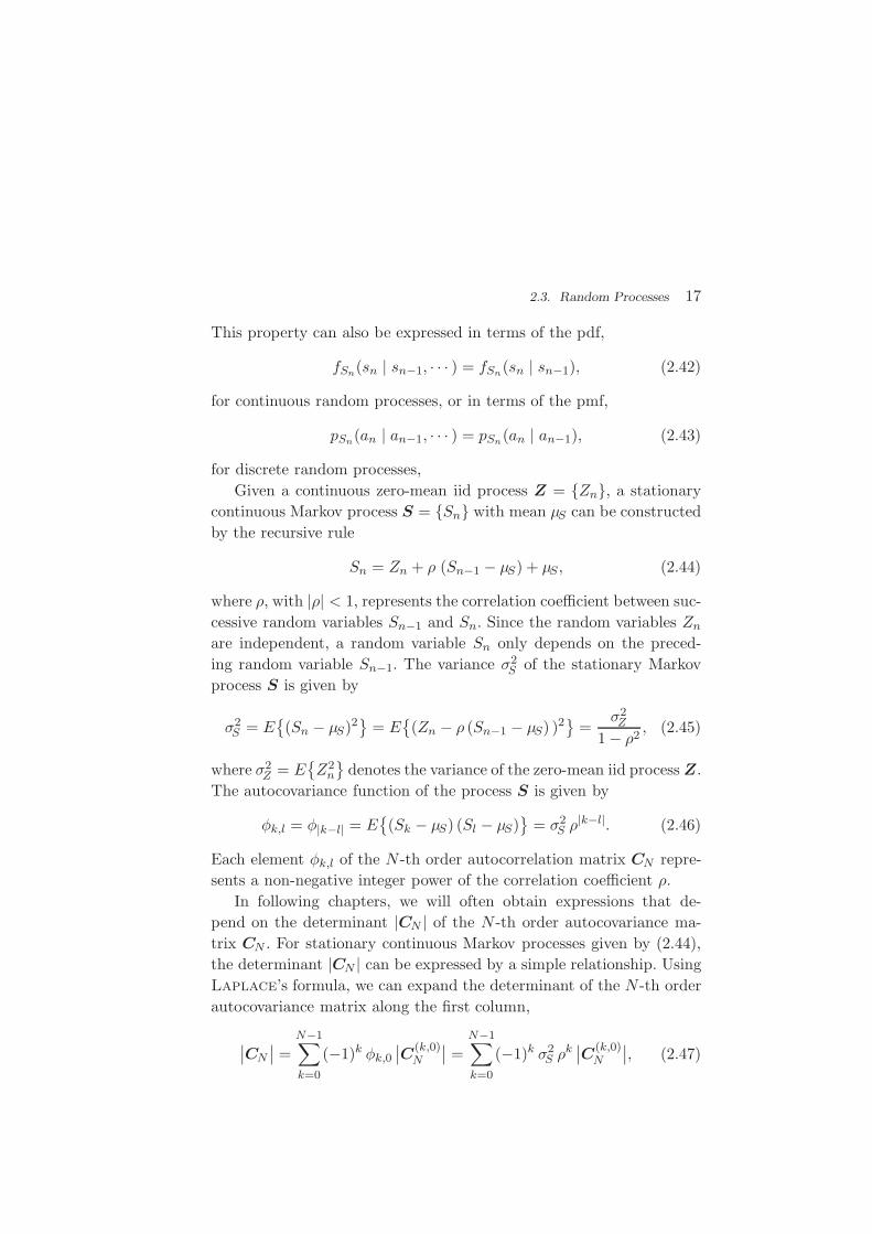
In following chapters, we will often obtain expressions that de-
pend on the determinant |CN | of the N -th order autocovariance ma-
trix CN . For stationary continuous Markov processes given by (2.44),
the determinant |CN | can be expressed by a simple relationship. Using
Laplace’s formula, we can expand the determinant of the N -th order
autocovariance matrix along the first column,
∣∣CN
∣∣ =
N−1∑
k=0
(−1)k φk,0
∣∣C
(k,0)N
∣∣ =
N−1∑
k=0
(−1)k σ2S ρk
∣∣C
(k,0)N
∣∣, (2.47)

18 Random Processes
where C(k,l)N represents the matrix that is obtained by removing the
k-th row and l-th column from CN . The first row of each matrix C(k,l)N ,
with k > 1, is equal to the second row of the same matrix multiplied by
the correlation coefficient ρ. Hence, the first two rows of these matrices
are linearly dependent and the determinants |C(k,l)N |, with k > 1, are
equal to 0. Thus, we obtain∣∣CN
∣∣ = σ2
S
∣∣C
(0,0)N
∣∣− σ2
S ρ∣∣C
(1,0)N
∣∣. (2.48)
The matrix C(0,0)N represents the autocovariance matrix CN−1 of the
order (N− 1). The matrix C(1,0)N is equal to CN−1 except that the first
row is multiplied by the correlation coefficient ρ. Hence, the determi-
nant |C(1,0)N | is equal to ρ |CN−1|, which yields the recursive rule
∣∣CN
∣∣ = σ2
S (1− ρ2)∣∣CN−1
∣∣. (2.49)
By using the expression |C1| = σ2S for the determinant of the 1-st order
autocovariance matrix, we obtain the relationship∣∣CN
∣∣ = σ2N
S (1− ρ2)N−1. (2.50)
2.3.2 Gaussian Processes
A continuous random process S={Sn} is said to be a Gaussian process
if all finite collections of random variables Sn represent Gaussian ran-
dom vectors. The N -th order pdf of a stationary Gaussian process S
with mean µS and variance σ2S is given by
fS(s) =1
(2π)N/2 |CN |1/2e−
12(s−µN )T C−1
N (s−µN ), (2.51)
where s is a vector of N consecutive samples, µN is the N -th order
mean (a vector with all N elements being equal to the mean µS), and
CN is an N -th order nonsingular autocovariance matrix given by (2.39).
2.3.3 Gauss-Markov Processes
A continuous random process is called a Gauss-Markov process if it
satisfies the requirements for both Gaussian processes and Markov
processes. The statistical properties of a stationary Gauss-Markov are

2.4. Summary of Random Processes 19
completely specified by its mean µS , its variance σ2S , and its correlation
coefficient ρ. The stationary continuous process in (2.44) is a stationary
Gauss-Markov process if the random variables Zn of the zero-mean iid
process Z have a Gaussian pdf fZ(s).
The N -th order pdf of a stationary Gauss-Markov process S with
the mean µS , the variance σ2S , and the correlation coefficient ρ is given
by (2.51), where the elements φk,l of the N -th order autocovariance
matrix CN depend on the variance σ2S and the correlation coefficient ρ
and are given by (2.46). The determinant |CN | of the N -th order auto-
covariance matrix of a stationary Gauss-Markov process can be written
according to (2.50).
2.4 Summary of Random Processes
In this chapter, we gave a brief review of the concepts of random vari-
ables and random processes. A random variable is a function of the
sample space of a random experiment. It assigns a real value to each
possible outcome of the random experiment. The statistical proper-
ties of random variables can be characterized by cumulative distribu-
tion functions (cdf’s), probability density functions (pdf’s), probability
mass functions (pmf’s), or expectation values.
Finite collections of random variables are called random vectors.
A countably infinite sequence of random variables is referred to as
(discrete-time) random process. Random processes for which the sta-
tistical properties are invariant to a shift in time are called stationary
processes. If the random variables of a process are independent, the
process is said to be memoryless. Random processes that are station-
ary and memoryless are also referred to as independent and identically
distributed (iid) processes. Important models for random processes,
which will also be used in this text, are Markov processes, Gaussian
processes, and Gauss-Markov processes.
Beside reviewing the basic concepts of random variables and random
processes, we also introduced the notations that will be used through-
out the text. For simplifying formulas in the following chapters, we will
often omit the subscripts that characterize the random variable(s) or
random vector(s) in the notations of cdf’s, pdf’s, and pmf’s.

3
Lossless Source Coding
Lossless source coding describes a reversible mapping of sequences of
discrete source symbols into sequences of codewords. In contrast to
lossy coding techniques, the original sequence of source symbols can be
exactly reconstructed from the sequence of codewords. Lossless coding
is also referred to as noiseless coding or entropy coding. If the origi-
nal signal contains statistical properties or dependencies that can be
exploited for data compression, lossless coding techniques can provide
a reduction in transmission rate. Basically all source codecs, and in
particular all video codecs, include a lossless coding part by which the
coding symbols are efficiently represented inside a bitstream.
In this chapter, we give an introduction to lossless source coding.
We analyze the requirements for unique decodability, introduce a fun-
damental bound for the minimum average codeword length per source
symbol that can be achieved with lossless coding techniques, and dis-
cuss various lossless source codes with respect to their efficiency, ap-
plicability, and complexity. For further information on lossless coding
techniques, the reader is referred to the overview of lossless compression
techniques in [67].
20

3.1. Classification of Lossless Source Codes 21
3.1 Classification of Lossless Source Codes
In this text, we restrict our considerations to the practically important
case of binary codewords. A codeword is a sequence of binary symbols
(bits) of the alphabet B={0, 1}. Let S={Sn} be a stochastic process
that generates sequences of discrete source symbols. The source sym-
bols sn are realizations of the random variables Sn. By the process of
lossless coding, a message s(L) ={s0, · · · , sL−1} consisting of L source
symbols is converted into a sequence b(K) ={b0, · · · , bK−1} of K bits.
In practical coding algorithms, a message s(L) is often split into
blocks s(N) = {sn, · · · , sn+N−1} of N symbols, with 1 ≤ N ≤ L, and
a codeword b(ℓ)(s(N)) = {b0, · · · , bℓ−1} of ℓ bits is assigned to each of
these blocks s(N). The length ℓ of a codeword bℓ(s(N)) can depend on
the symbol block s(N). The codeword sequence b(K) that represents the
message s(L) is obtained by concatenating the codewords bℓ(s(N)) for
the symbol blocks s(N). A lossless source code can be described by the
encoder mapping
b(ℓ) = γ(s(N)
), (3.1)
which specifies a mapping from the set of finite length symbol blocks
to the set of finite length binary codewords. The decoder mapping
s(N) = γ−1(b(ℓ)
)= γ−1
(γ(s(N)
) )(3.2)
is the inverse of the encoder mapping γ.
Depending on whether the number N of symbols in the blocks s(N)
and the number ℓ of bits for the associated codewords are fixed or
variable, the following categories can be distinguished:
(1) Fixed-to-fixed mapping: A fixed number of symbols is mapped
to fixed length codewords. The assignment of a fixed num-
ber ℓ of bits to a fixed number N of symbols yields a codeword
length of ℓ/N bit per symbol. We will consider this type of
lossless source codes as a special case of the next type.
(2) Fixed-to-variable mapping: A fixed number of symbols is
mapped to variable length codewords. A well-known method
for designing fixed-to-variable mappings is the Huffman al-
gorithm for scalars and vectors, which we will describe in
sec. 3.2 and sec. 3.3, respectively.

22 Lossless Source Coding
(3) Variable-to-fixed mapping: A variable number of symbols is
mapped to fixed length codewords. An example for this type
of lossless source codes are Tunstall codes [73, 66]. We will
not further describe variable-to-fixed mappings in this text,
because of its limited use in video coding.
(4) Variable-to-variable mapping: A variable number of symbols
is mapped to variable length codewords. A typical example
for this type of lossless source codes are arithmetic codes,
which we will describe in sec. 3.4. As a less-complex alterna-
tive to arithmetic coding, we will also present the probability
interval projection entropy code in sec. 3.5.
3.2 Variable-Length Coding for Scalars
In this section, we consider lossless source codes that assign a sepa-
rate codeword to each symbol sn of a message s(L). It is supposed that
the symbols of the message s(L) are generated by a stationary discrete
random process S = {Sn}. The random variables Sn = S are character-
ized by a finite1 symbol alphabet A = {a0, · · · , aM−1} and a marginal
pmf p(a) = P (S = a). The lossless source code associates each letter ai
of the alphabet A with a binary codeword bi = {bi0, · · · , bi
ℓ(ai)−1} of a
length ℓ(ai) ≥ 1. The goal of the lossless code design is to minimize the
average codeword length
ℓ = E{ℓ(S)} =M−1∑
i=0
p(ai) ℓ(ai), (3.3)
while ensuring that each message s(L) is uniquely decodable given their
coded representation b(K).
3.2.1 Unique Decodability
A code is said to be uniquely decodable if and only if each valid coded
representation b(K) of a finite number K of bits can be produced by
only one possible sequence of source symbols s(L).
1 The fundamental concepts and results shown in this section are also valid for countablyinfinite symbol alphabets (M → ∞).

3.2. Variable-Length Coding for Scalars 23
A necessary condition for unique decodability is that each letter ai
of the symbol alphabetA is associated with a different codeword. Codes
with this property are called non-singular codes and ensure that a single
source symbol is unambiguously represented. But if messages with more
than one symbol are transmitted, non-singularity is not sufficient to
guarantee unique decodability, as will be illustrated in the following.
ai p(ai) code A code B code C code D code E
a0 0.5 0 0 0 00 0a1 0.25 10 01 01 01 10a2 0.125 11 010 011 10 110a3 0.125 11 011 111 110 111
ℓ 1.5 1.75 1.75 2.125 1.75
Table 3.1 Example codes for a source with a four letter alphabet and a given marginal pmf.
Table 3.1 shows five example codes for a source with a four letter
alphabet and a given marginal pmf. Code A has the smallest average
codeword length, but since the symbols a2 and a3 cannot be distin-
guished2. Code A is a singular code and is not uniquely decodable.
Although code B is a non-singular code, it is not uniquely decodable ei-
ther, since the concatenation of the letters a1 and a0 produces the same
bit sequence as the letter a2. The remaining three codes are uniquely
decodable, but differ in other properties. While code D has an average
codeword length of 2.125 bit per symbol, the codes C and E have an
average codeword length of only 1.75 bit per symbol, which is, as we
will show later, the minimum achievable average codeword length for
the given source. Beside being uniquely decodable, the codes D and E
are also instantaneously decodable, i.e., each alphabet letter can be de-
coded right after the bits of its codeword are received. The code C does
not have this property. If a decoder for the code C receives a bit equal
to 0, it has to wait for the next bit equal to 0 before a symbol can be
decoded. Theoretically, the decoder might need to wait until the end
of the message. The value of the next symbol depends on how many
bits equal to 1 are received between the zero bits.
2 This may be a desirable feature in lossy source coding systems as it helps to reduce thetransmission rate, but in this section, we concentrate on lossless source coding. Note thatthe notation γ is only used for unique and invertible mappings throughout this text.

24 Lossless Source Coding
‘ 0 ’
‘ 0 ’
‘ 0 ’
‘ 0 ’
’ 10 ’
‘ 1 ’
‘ 1 ’
‘ 1 ’ ‘ 110 ’
‘ 111 ’
root node
interior node
terminal node
branch
‘ 0 ’
‘ 0 ’
‘ 0 ’
‘ 0 ’
’ 10 ’
‘ 1 ’
‘ 1 ’
‘ 1 ’ ‘ 110 ’
‘ 111 ’
root node
interior node
terminal node
branch
Fig. 3.1 Example for a binary code tree. The represented code is code E of Table 3.1.
Binary Code Trees. Binary codes can be represented using binary
trees as illustrated in Fig. 3.1. A binary tree is a data structure that
consists of nodes, with each node having zero, one, or two descendant
nodes. A node and its descendants nodes are connected by branches. A
binary tree starts with a root node, which is the only node that is not
a descendant of any other node. Nodes that are not the root node but
have descendants are referred to as interior nodes, whereas nodes that
do not have descendants are called terminal nodes or leaf nodes.
In a binary code tree, all branches are labeled with ‘0’ or ‘1’. If
two branches depart from the same node, they have different labels.
Each node of the tree represents a codeword, which is given by the
concatenation of the branch labels from the root node to the considered
node. A code for a given alphabet A can be constructed by associating
all terminal nodes and zero or more interior nodes of a binary code tree
with one or more alphabet letters. If each alphabet letter is associated
with a distinct node, the resulting code is non-singular. In the example
of Fig. 3.1, the nodes that represent alphabet letters are filled.
Prefix Codes. A code is said to be a prefix code if no codeword for
an alphabet letter represents the codeword or a prefix of the codeword
for any other alphabet letter. If a prefix code is represented by a binary
code tree, this implies that each alphabet letter is assigned to a distinct
terminal node, but not to any interior node. It is obvious that every
prefix code is uniquely decodable. Furthermore, we will prove later
that for every uniquely decodable code there exists a prefix code with
exactly the same codeword lengths. Examples for prefix codes are the
codes D and E in Table 3.1.

3.2. Variable-Length Coding for Scalars 25
Based on the binary code tree representation the parsing rule for
prefix codes can be specified as follows:
(1) Set the current node ni equal to the root node.
(2) Read the next bit b from the bitstream.
(3) Follow the branch labeled with the value of b from the current
node ni to the descendant node nj.
(4) If nj is a terminal node, return the associated alphabet letter
and proceed with step 1. Otherwise, set the current node ni
equal to nj and repeat the previous two steps.
The parsing rule reveals that prefix codes are not only uniquely de-
codable, but also instantaneously decodable. As soon as all bits of a
codeword are received, the transmitted symbol is immediately known.
Due to this property, it is also possible to switch between different
independently designed prefix codes inside a bitstream (i.e., because
symbols with different alphabets are interleaved according to a given
bitstream syntax) without impacting the unique decodability.
Kraft Inequality. A necessary condition for uniquely decodable
codes is given by the Kraft inequality,
M−1∑
i=0
2−ℓ(ai) ≤ 1. (3.4)
For proving this inequality, we consider the term
(M−1∑
i=0
2−ℓ(ai)
)L
=
M−1∑
i0=0
M−1∑
i1=0
· · ·M−1∑
iL−1=0
2−(ℓ(ai0
)+ℓ(ai1)+···+ℓ(aiL−1
))
. (3.5)
The term ℓL = ℓ(ai0) + ℓ(ai1) + · · ·+ ℓ(aiL−1) represents the combined
codeword length for coding L symbols. Let A(ℓL) denote the number of
distinct symbol sequences that produce a bit sequence with the same
length ℓL. A(ℓL) is equal to the number of terms 2−ℓL that are contained
in the sum of the right side of (3.5). For a uniquely decodable code,
A(ℓL) must be less than or equal to 2ℓL , since there are only 2ℓL distinct
bit sequences of length ℓL. If the maximum length of a codeword is ℓmax,

26 Lossless Source Coding
the combined codeword length ℓL lies inside the interval [L,L · ℓmax].
Hence, a uniquely decodable code must fulfill the inequality(
M−1∑
i=0
2−ℓ(ai)
)L
=L·ℓmax∑
ℓL=L
A(ℓL) 2−ℓL ≤L·ℓmax∑
ℓL=L
2ℓL 2−ℓL = L (ℓmax− 1) + 1.
(3.6)
The left side of this inequality grows exponentially with L, while the
right side grows only linearly with L. If the Kraft inequality (3.4) is not
fulfilled, we can always find a value of L for which the condition (3.6)
is violated. And since the constraint (3.6) must be obeyed for all values
of L ≥ 1, this proves that the Kraft inequality specifies a necessary
condition for uniquely decodable codes.
The Kraft inequality does not only provide a necessary condi-
tion for uniquely decodable codes, it is also always possible to con-
struct a uniquely decodable code for any given set of codeword lengths
{ℓ0, ℓ1, · · · , ℓM−1} that satisfies the Kraft inequality. We prove this
statement for prefix codes, which represent a subset of uniquely de-
codable codes. Without loss of generality, we assume that the given
codeword lengths are ordered as ℓ0 ≤ ℓ1 ≤ · · · ≤ ℓM−1. Starting with an
infinite binary code tree, we chose an arbitrary node of depth ℓ0 (i.e., a
node that represents a codeword of length ℓ0) for the first codeword and
prune the code tree at this node. For the next codeword length ℓ1, one
of the remaining nodes with depth ℓ1 is selected. A continuation of this
procedure yields a prefix code for the given set of codeword lengths, un-
less we cannot select a node for a codeword length ℓi because all nodes
of depth ℓi have already been removed in previous steps. It should be
noted that the selection of a codeword of length ℓk removes 2ℓi−ℓk code-
words with a length of ℓi ≥ ℓk. Consequently, for the assignment of a
codeword length ℓi, the number of available codewords is given by
n(ℓi) = 2ℓi −i−1∑
k=0
2ℓi−ℓk = 2ℓi
(
1−i−1∑
k=0
2−ℓk
)
. (3.7)
If the Kraft inequality (3.4) is fulfilled, we obtain
n(ℓi) ≥ 2ℓi
(M−1∑
k=0
2−ℓk −i−1∑
k=0
2−ℓk
)
= 1 +
M−1∑
k=i+1
2−ℓk ≥ 1. (3.8)

3.2. Variable-Length Coding for Scalars 27
Hence, it is always possible to construct a prefix code, and thus a
uniquely decodable code, for a given set of codeword lengths that sat-
isfies the Kraft inequality.
The proof shows another important property of prefix codes. Since
all uniquely decodable codes fulfill the Kraft inequality and it is always
possible to construct a prefix code for any set of codeword lengths that
satisfies the Kraft inequality, there do not exist uniquely decodable
codes that have a smaller average codeword length than the best prefix
code. Due to this property and since prefix codes additionally provide
instantaneous decodability and are easy to construct, all variable length
codes that are used in practice are prefix codes.
3.2.2 Entropy
Based on the Kraft inequality, we now derive a lower bound for the
average codeword length of uniquely decodable codes. The expression
(3.3) for the average codeword length ℓ can be rewritten as
ℓ =M−1∑
i=0
p(ai) ℓ(ai) = −M−1∑
i=0
p(ai) log2
(
2−ℓ(ai)
p(ai)
)
−M−1∑
i=0
p(ai) log2 p(ai).
(3.9)
With the definition q(ai) = 2−ℓ(ai)/(∑M−1
k=0 2−ℓ(ak))
, we obtain
ℓ = − log2
(M−1∑
i=0
2−ℓ(ai)
)
−M−1∑
i=0
p(ai) log2
(q(ai)
p(ai)
)
−M−1∑
i=0
p(ai) log2 p(ai).
(3.10)
Since the Kraft inequality is fulfilled for all uniquely decodable codes,
the first term on the right side of (3.10) is greater than or equal to 0.
The second term is also greater than or equal to 0 as can be shown
using the inequality ln x ≤ x− 1 (with equality if and only if x = 1),
−M−1∑
i=0
p(ai) log2
(q(ai)
p(ai)
)
≥ 1
ln 2
M−1∑
i=0
p(ai)
(
1− q(ai)
p(ai)
)
=1
ln 2
(M−1∑
i=0
p(ai)−M−1∑
i=0
q(ai)
)
= 0. (3.11)

28 Lossless Source Coding
The inequality (3.11) is also referred to as divergence inequality for
probability mass functions. The average codeword length ℓ for uniquely
decodable codes is bounded by
ℓ ≥ H(S) (3.12)
with
H(S) = E{− log2 p(S)} = −M−1∑
i=0
p(ai) log2 p(ai). (3.13)
The lower bound H(S) is called the entropy of the random variable S
and does only depend on the associated pmf p. Often the entropy of a
random variable with a pmf p is also denoted as H(p). The redundancy
of a code is given by the difference
= ℓ−H(S) ≥ 0. (3.14)
The entropy H(S) can also be considered as a measure for the uncer-
tainty3 that is associated with the random variable S.
The inequality (3.12) is an equality if and only if the first and second
term on the right side of (3.10) are equal to 0. This is only the case if
the Kraft inequality is fulfilled with equality and q(ai) = p(ai), ∀ai∈A.
The resulting conditions ℓ(ai) = − log2 p(ai), ∀ai∈A, can only hold if
all alphabet letters have probabilities that are integer powers of 1/2.
For deriving an upper bound for the minimum average codeword
length we choose ℓ(ai) = ⌈− log2 p(ai)⌉, ∀ai ∈ A, where ⌈x⌉ represents
the smallest integer greater than or equal to x. Since these codeword
lengths satisfy the Kraft inequality, as can be shown using ⌈x⌉ ≥ x,
M−1∑
i=0
2−⌈− log2 p(ai)⌉ ≤M−1∑
i=0
2log2 p(ai) =
M−1∑
i=0
p(ai) = 1, (3.15)
we can always construct a uniquely decodable code. For the average
codeword length of such a code, we obtain, using ⌈x⌉ < x + 1,
ℓ =
M−1∑
i=0
p(ai) ⌈− log2 p(ai)⌉ <
M−1∑
i=0
p(ai) (1− log2 p(ai)) = H(S) + 1.
(3.16)
3 In Shannon’s original paper [69], the entropy was introduced as an uncertainty measurefor random experiments and was derived based on three postulates for such a measure.
3.2. Variable-Length Coding for Scalars 29
The minimum average codeword length ℓmin that can be achieved with
uniquely decodable codes that assign a separate codeword to each letter
of an alphabet always satisfies the inequality
H(S) ≤ ℓmin < H(S) + 1. (3.17)
The upper limit is approached for a source with a two-letter alphabet
and a pmf {p, 1− p} if the letter probability p approaches 0 or 1 [15].
3.2.3 The Huffman Algorithm
For deriving an upper bound for the minimum average codeword length
we chose ℓ(ai) = ⌈− log2 p(ai)⌉, ∀ai ∈ A. The resulting code has a re-
dundancy = ℓ−H(Sn) that is always less than 1 bit per symbol, but
it does not necessarily achieve the minimum average codeword length.
For developing an optimal uniquely decodable code, i.e., a code that
achieves the minimum average codeword length, it is sufficient to con-
sider the class of prefix codes, since for every uniquely decodable code
there exists a prefix code with the exactly same codeword length. An
optimal prefix code has the following properties:
• For any two symbols ai, aj ∈ A with p(ai)> p(aj), the asso-
ciated codeword lengths satisfy ℓ(ai) ≤ ℓ(aj).
• There are always two codewords that have the maximum
codeword length and differ only in the final bit.
These conditions can be proved as follows. If the first condition is not
fulfilled, an exchange of the codewords for the symbols ai and aj would
decrease the average codeword length while preserving the prefix prop-
erty. And if the second condition is not satisfied, i.e., if for a particular
codeword with the maximum codeword length there does not exist a
codeword that has the same length and differs only in the final bit, the
removal of the last bit of the particular codeword would preserve the
prefix property and decrease the average codeword length.
Both conditions for optimal prefix codes are obeyed if two code-
words with the maximum length that differ only in the final bit are
assigned to the two letters ai and aj with the smallest probabilities.
In the corresponding binary code tree, a parent node for the two leaf
30 Lossless Source Coding
nodes that represent these two letters is created. The two letters ai and
aj can then be treated as a new letter with a probability of p(ai)+p(aj)
and the procedure of creating a parent node for the nodes that repre-
sent the two letters with the smallest probabilities can be repeated for
the new alphabet. The resulting iterative algorithm was developed and
proved to be optimal by Huffman in [30]. Based on the construction
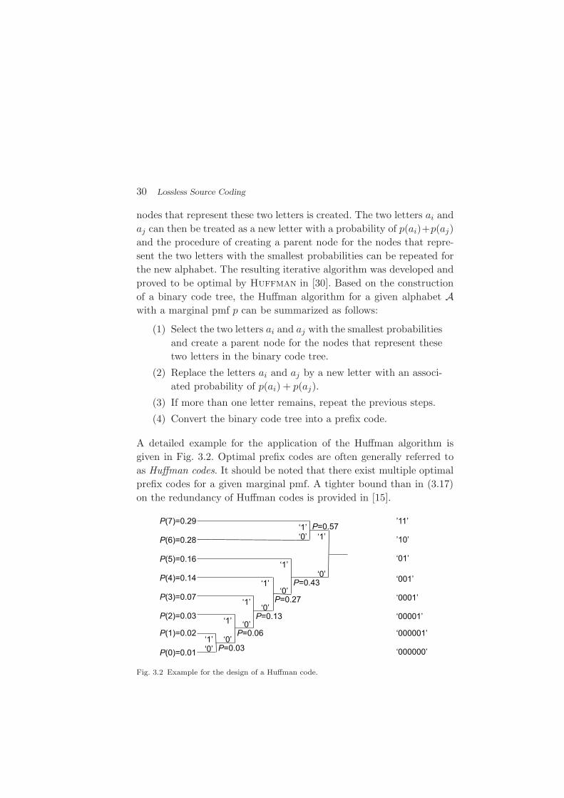
of a binary code tree, the Huffman algorithm for a given alphabet Awith a marginal pmf p can be summarized as follows:
(1) Select the two letters ai and aj with the smallest probabilities
and create a parent node for the nodes that represent these
two letters in the binary code tree.
(2) Replace the letters ai and aj by a new letter with an associ-
ated probability of p(ai) + p(aj).
(3) If more than one letter remains, repeat the previous steps.
(4) Convert the binary code tree into a prefix code.
A detailed example for the application of the Huffman algorithm is
given in Fig. 3.2. Optimal prefix codes are often generally referred to
as Huffman codes. It should be noted that there exist multiple optimal
prefix codes for a given marginal pmf. A tighter bound than in (3.17)
on the redundancy of Huffman codes is provided in [15].
P=0.03 ‘0’ ‘1’
P=0.06 ‘0’
‘1’ P=0.13
‘0’
‘1’ P=0.27 ‘0’
‘1’ P=0.43 ‘0’
‘1’
P=0.57
‘0’‘1’
‘0’
‘1’
P(7)=0.29
P(6)=0.28
P(5)=0.16
P(4)=0.14
P(3)=0.07
P(2)=0.03
P(1)=0.02
P(0)=0.01
’11’
’10’
‘01’
‘001’
‘0001’
‘00001’
‘000001’
‘000000’
Fig. 3.2 Example for the design of a Huffman code.

3.2. Variable-Length Coding for Scalars 31
3.2.4 Conditional Huffman Codes
Until now, we considered the design of variable length codes for the
marginal pmf of stationary random processes. However, for random
processes {Sn} with memory, it can be beneficial to design variable
length codes for conditional pmfs and switch between multiple code-
word tables depending on already coded symbols.
a a0 a1 a2 entropy
p(a|a0) 0.90 0.05 0.05 H(Sn|a0) = 0.5690
p(a|a1) 0.15 0.80 0.05 H(Sn|a1) = 0.8842
p(a|a2) 0.25 0.15 0.60 H(Sn|a2) = 1.3527
p(a) 0.64 0.24 0.1 H(S) = 1.2575
Table 3.2 Conditional pmfs p(a|ak) and conditional entropies H(Sn|ak) for an example ofa stationary discrete Markov process with a three letter alphabet. The conditional entropyH(Sn|ak) is the entropy of the conditional pmf p(a|ak) given the event {Sn−1 = ak}. Theresulting marginal pmf p(a) and marginal entropy H(S) are given in the last table row.
As an example, we consider a stationary discrete Markov process
with a three symbol alphabet A = {a0, a1, a2}. The statistical proper-
ties of this process are completely characterized by three conditional
pmfs p(a|ak) = P (Sn =a |Sn−1 =ak) with k = 0, 1, 2, which are given
in Table 3.2. An optimal prefix code for a given conditional pmf can be
designed in exactly the same way as for a marginal pmf. A correspond-
ing Huffman code design for the example Markov source is shown in
Table 3.3. For comparison, Table 3.3 lists also a Huffman code for the
marginal pmf. The codeword table that is chosen for coding a symbol sn
depends on the value of the preceding symbol sn−1. It is important to
note that an independent code design for the conditional pmfs is only
possible for instantaneously decodable codes, i.e., for prefix codes.
aiHuffman codes for conditional pmfs Huffman code
for marginal pmfSn−1 = a0 Sn−1 = a2 Sn−1 = a2
a0 1 00 00 1a1 00 1 01 00a2 01 01 1 01
ℓ 1.1 1.2 1.4 1.3556
Table 3.3 Huffman codes for the conditional pmfs and the marginal pmf of the Markovprocess specified in Table 3.2.

32 Lossless Source Coding
The average codeword length ℓk = ℓ(Sn−1 =ak) of an optimal prefix
code for each of the conditional pmfs is guaranteed to lie in the half-
open interval [H(Sn|ak),H(Sn|ak) + 1), where
H(Sn|ak) = H(Sn|Sn−1 =ak) = −M−1∑
i=0
p(ai|ak) log2 p(ai|ak) (3.18)
denotes the conditional entropy of the random variable Sn given the
event {Sn−1 = ak}. The resulting average codeword length ℓ for the
conditional code is
ℓ =
M−1∑
k=0
p(ak) ℓk. (3.19)
The resulting lower bound for the average codeword length ℓ is referred
to as the conditional entropy H(Sn|Sn−1) of the random variable Sn
assuming the random variable Sn−1 and is given by
H(Sn|Sn−1) = E{− log2 p(Sn|Sn−1)} =
M−1∑
k=0
p(ak)H(Sn|Sn−1 =ak)
= −M−1∑
i=0
M−1∑
k=0
p(ai, ak) log2 p(ai|ak), (3.20)
where p(ai, ak) = P (Sn =ai, Sn−1 =ak) denotes the joint pmf of the
random variables Sn and Sn−1. The conditional entropy H(Sn|Sn−1)
specifies a measure for the uncertainty about Sn given the value of Sn−1.
The minimum average codeword length ℓmin that is achievable with the
conditional code design is bounded by
H(Sn|Sn−1) ≤ ℓmin < H(Sn|Sn−1) + 1. (3.21)
As can be easily shown from the divergence inequality (3.11),
H(S)−H(Sn|Sn−1) = −M−1∑
i=0
M−1∑
k=0
p(ai, ak)(
log2 p(ai)− log2 p(ai|ak))
= −M−1∑
i=0
M−1∑
k=0
p(ai, ak) log2p(ai) p(ak)
p(ai, ak)
≥ 0, (3.22)

3.3. Variable-Length Coding for Vectors 33
the conditional entropy H(Sn|Sn−1) is always less than or equal to the
marginal entropy H(S). Equality is obtained if p(ai, ak) = p(ai)p(ak),
∀ai, ak ∈ A, i.e., if the stationary process S is an iid process.
For our example, the average codeword length of the conditional
code design is 1.1578 bit per symbol, which is about 14.6% smaller than
the average codeword length of the Huffman code for the marginal pmf.
For sources with memory that do not satisfy the Markov property,
it can be possible to further decrease the average codeword length if
more than one preceding symbol is used in the condition. However, the
number of codeword tables increases exponentially with the number
of considered symbols. To reduce the number of tables, the number of
outcomes for the condition can be partitioned into a small number of
events, and for each of these events, a separate code can be designed.
As an application example, the CAVLC design in the H.264/AVC video
coding standard [36] includes conditional variable length codes.
3.2.5 Adaptive Huffman Codes
In practice, the marginal and conditional pmfs of a source are usu-
ally not known and sources are often nonstationary. Conceptually, the
pmf(s) can be simultaneously estimated in encoder and decoder and a
Huffman code can be redesigned after coding a particular number of
symbols. This would, however, tremendously increase the complexity
of the coding process. A fast algorithm for adapting Huffman codes
was proposed by Gallager [15]. But even this algorithm is considered
as too complex for video coding application, so that adaptive Huffman
codes are rarely used in this area.
3.3 Variable-Length Coding for Vectors
Although scalar Huffman codes achieve the smallest average codeword
length among all uniquely decodable codes that assign a separate code-
word to each letter of an alphabet, they can be very inefficient if there
are strong dependencies between the random variables of a process.
For sources with memory, the average codeword length per symbol can
be decreased if multiple symbols are coded jointly. Huffman codes that
assign a codeword to a block of two or more successive symbols are

34 Lossless Source Coding
referred to as block Huffman codes or vector Huffman codes and repre-
sent an alternative to conditional Huffman codes4. The joint coding of
multiple symbols is also advantageous for iid processes for which one
of the probabilities masses is close to one.
3.3.1 Huffman Codes for Fixed-Length Vectors
We consider stationary discrete random sources S = {Sn} with an
M -ary alphabet A = {a0, · · · , aM−1}. If N symbols are coded jointly,
the Huffman code has to be designed for the joint pmf
p(a0, · · · , aN−1) = P (Sn =a0, · · · , Sn+N−1 =aN−1)
of a block of N successive symbols. The average codeword length ℓmin
per symbol for an optimum block Huffman code is bounded by
H(Sn, · · · , Sn+N−1)
N≤ ℓmin <
H(Sn, · · · , Sn+N−1)
N+
1
N, (3.23)
where
H(Sn, · · · , Sn+N−1) = E{− log2 p(Sn, · · · , Sn+N−1)} (3.24)
is referred to as the block entropy for a set of N successive random
variables {Sn, · · · , Sn+N−1}. The limit
H(S) = limN→∞
H(S0, · · · , SN−1)
N(3.25)
is called the entropy rate of a source S. It can be shown that the limit in
(3.25) always exists for stationary sources [14]. The entropy rate H(S)
represents the greatest lower bound for the average codeword length ℓ
per symbol that can be achieved with lossless source coding techniques,
ℓ ≥ H(S). (3.26)
For iid processes, the entropy rate
H(S) = limN→∞
E{− log2 p(S0, S1, · · · , SN−1)}N
= limN→∞
∑N−1n=0 E{− log2 p(Sn)}
N= H(S) (3.27)
4 The concepts of conditional and block Huffman codes can also be combined by switchingcodeword tables for a block of symbols depending on the values of already coded symbols.

3.3. Variable-Length Coding for Vectors 35
is equal to the marginal entropy H(S). For stationary Markov pro-
cesses, the entropy rate
H(S) = limN→∞
E{− log2 p(S0, S1, · · · , SN−1)}N
= limN→∞
E{− log2 p(S0)}+∑N−1
n=1 E{− log2 p(Sn|Sn−1)}N
= H(Sn|Sn+1) (3.28)
is equal to the conditional entropy H(Sn|Sn−1).
aiak p(ai, ak) codewords
a0a0 0.58 1a0a1 0.032 00001a0a2 0.032 00010a1a0 0.036 0010a1a1 0.195 01a1a2 0.012 000000a2a0 0.027 00011a2a1 0.017 000001
(a) a2a2 0.06 0011
N ℓ NC
1 1.3556 32 1.0094 93 0.9150 274 0.8690 815 0.8462 2436 0.8299 7297 0.8153 21878 0.8027 6561
(b) 9 0.7940 19683
Table 3.4 Block Huffman codes for the Markov source specified in Table 3.2: (a) Huffmancode for a block of 2 symbols; (b) Average codeword lengths ℓ and number NC of codewordsdepending on the number N of jointly coded symbols.
As an example for the design of block Huffman codes, we con-
sider the discrete Markov process specified in Table 3.2. The entropy
rate H(S) for this source is 0.7331 bit per symbol. Table 3.4(a) shows
a Huffman code for the joint coding of 2 symbols. The average code-
word length per symbol for this code is 1.0094 bit per symbol, which is
smaller than the average codeword length obtained with the Huffman
code for the marginal pmf and the conditional Huffman code that we
developed in sec. 3.2. As shown in Table 3.4(b), the average codeword
length can be further reduced by increasing the number N of jointly
coded symbols. If N approaches infinity, the average codeword length
per symbol for the block Huffman code approaches the entropy rate.
However, the number NC of codewords that must be stored in an en-
coder and decoder grows exponentially with the number N of jointly
coded symbols. In practice, block Huffman codes are only used for a
small number of symbols with small alphabets.

36 Lossless Source Coding
In general, the number of symbols in a message is not a multiple of
the block size N . The last block of source symbols may contain less than
N symbols, and, in that case, it cannot be represented with the block
Huffman code. If the number of symbols in a message is known to the
decoder (e.g., because it is determined by a given bitstream syntax), an
encoder can send the codeword for any of the letter combinations that
contain the last block of source symbols as a prefix. At the decoder
side, the additionally decoded symbols are discarded. If the number of
symbols that are contained in a message cannot be determined in the
decoder, a special symbol for signaling the end of a message can be
added to the alphabet.
3.3.2 Huffman Codes for Variable-Length Vectors
An additional degree of freedom for designing Huffman codes, or gen-
erally variable-length codes, for symbol vectors is obtained if the re-
striction that all codewords are assigned to symbol blocks of the same
size is removed. Instead, the codewords can be assigned to sequences
of a variable number of successive symbols. Such a code is also referred
to as V2V code in this text. In order to construct a V2V code, a set
of letter sequences with a variable number of letters is selected and
a codeword is associated with each of these letter sequences. The set
of letter sequences has to be chosen in a way that each message can
be represented by a concatenation of the selected letter sequences. An
exception is the end of a message, for which the same concepts as for
block Huffman codes (see above) can be used.
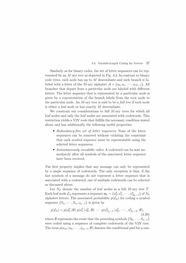
Fig. 3.3 Example for an M -ary tree representing sequences of a variable number of letters,of the alphabet A = {a0, a1, a2}, with an associated variable length code.
3.3. Variable-Length Coding for Vectors 37
Similarly as for binary codes, the set of letter sequences can be rep-
resented by an M -ary tree as depicted in Fig. 3.3. In contrast to binary
code trees, each node has up to M descendants and each branch is la-
beled with a letter of the M -ary alphabet A = {a0, a1, · · · , aM−1}. All
branches that depart from a particular node are labeled with different
letters. The letter sequence that is represented by a particular node is
given by a concatenation of the branch labels from the root node to
the particular node. An M -ary tree is said to be a full tree if each node
is either a leaf node or has exactly M descendants.
We constrain our considerations to full M -ary trees for which all
leaf nodes and only the leaf nodes are associated with codewords. This
restriction yields a V2V code that fulfills the necessary condition stated
above and has additionally the following useful properties:
• Redundancy-free set of letter sequences: None of the letter
sequences can be removed without violating the constraint
that each symbol sequence must be representable using the
selected letter sequences.
• Instantaneously encodable codes: A codeword can be sent im-
mediately after all symbols of the associated letter sequence
have been received.
The first property implies that any message can only be represented
by a single sequence of codewords. The only exception is that, if the
last symbols of a message do not represent a letter sequence that is
associated with a codeword, one of multiple codewords can be selected
as discussed above.
Let NL denote the number of leaf nodes in a full M -ary tree T .
Each leaf node Lk represents a sequence ak = {ak0 , a
k1 , · · · , ak
Nk−1} of Nk
alphabet letters. The associated probability p(Lk) for coding a symbol
sequence {Sn, · · · , Sn+Nk−1} is given by
p(Lk) = p(ak0 | B) p(ak
1 | ak0 , B) · · · p(ak
Nk−1 | ak0 , · · · , ak
Nk−2, B),
(3.29)
where B represents the event that the preceding symbols {S0, . . . , Sn−1}were coded using a sequence of complete codewords of the V2V tree.
The term p(am | a0, · · · , am−1,B) denotes the conditional pmf for a ran-

38 Lossless Source Coding
dom variable Sn+m given the random variables Sn to Sn+m−1 and the
event B. For iid sources, the probability p(Lk) for a leaf node Lk sim-
plifies to
p(Lk) = p(ak0) p(ak
1) · · · p(akNk−1). (3.30)
For stationary Markov sources, the probabilities p(Lk) are given by
p(Lk) = p(ak0 | B) p(ak
1 | ak0) · · · p(ak
Nk−1 | akNk−2). (3.31)
The conditional pmfs p(am | a0, · · · , am−1,B) are given by the structure
of the M -ary tree T and the conditional pmfs p(am | a0, · · · , am−1) for
the random variables Sn+m assuming the preceding random variables
Sn to Sn+m−1.
As an example, we show how the pmf p(a|B) = P (Sn =a|B) that is
conditioned on the event B can be determined for Markov sources. In
this case, the probability p(am|B) = P (Sn =am|B) that a codeword is
assigned to a letter sequence that starts with a particular letter am of
the alphabet A = {a0, a1, · · · , aM−1} is given by
p(am|B) =
NL−1∑
k=0
p(am|akNk−1) p(ak
Nk−1|akNk−2) · · · p(ak
1 |ak0) p(ak
0 |B).
(3.32)
These M equations form a homogeneous linear equation system that
has one set of non-trivial solutions p(a|B) = κ · {x0, x1, · · · , xM−1}. The
scale factor κ and thus the pmf p(a|B) can be uniquely determined by
using the constraint∑M−1
m=0 p(am|B) = 1.
After the conditional pmfs p(am | a0, · · · , am−1,B) have been deter-
mined, the pmf p(L) for the leaf nodes can be calculated. An optimal
prefix code for the selected set of letter sequences, which is represented
by the leaf nodes of a full M -ary tree T , can be designed using the
Huffman algorithm for the pmf p(L). Each leaf node Lk is associated
with a codeword of ℓk bits. The average codeword length per symbol ℓ
is given by the ratio of the average codeword length per letter sequence
and the average number of letters per letter sequence,
ℓ =
∑NL−1k=0 p(Lk) ℓk
∑NL−1k=0 p(Lk)Nk
. (3.33)

3.3. Variable-Length Coding for Vectors 39
For selecting the set of letter sequences or the full M -ary tree T , we
assume that the set of applicable V2V codes for an application is given
by parameters such as the maximum number of codewords (number of
leaf nodes). Given such a finite set of full M -ary trees, we can select
the full M -ary tree T , for which the Huffman code yields the smallest
average codeword length per symbol ℓ.
ak p(Lk) codewords
a0a0 0.5799 1a0a1 0.0322 00001a0a2 0.0322 00010a1a0 0.0277 00011a1a1a0 0.0222 000001a1a1a1 0.1183 001a1a1a2 0.0074 0000000a1a2 0.0093 0000001
(a) a2 0.1708 01
NC ℓ
5 1.17847 1.05519 1.0049
11 0.973313 0.941215 0.929317 0.907419 0.8980
(b) 21 0.8891
Table 3.5 V2V codes for the Markov source specified in Table 3.2: (a) V2V code with NC = 9codewords; (b) Average codeword lengths ℓ depending on the number of codewords NC .
As an example for the design of a V2V Huffman code, we again
consider the stationary discrete Markov source specified in Table 3.2.
Table 3.5(a) shows a V2V code that minimizes the average codeword
length per symbol among all V2V codes with up to 9 codewords. The
average codeword length is 1.0049 bit per symbol, which is about 0.4%
smaller than the average codeword length for the block Huffman code
with the same number of codewords. As indicated in Table 3.5(b), when
increasing the number of codewords, the average codeword length for
V2V codes usually decreases faster as for block Huffman codes. The
V2V code with 17 codewords has already an average codeword length
that is smaller than that of the block Huffman code with 27 codewords.
An application example of V2V codes is the run-level coding of
transform coefficients in MPEG-2 Video [39]. An often used variation of
V2V codes is called run-length coding. In run-length coding, the number
of successive occurrences of a particular alphabet letter, referred to as
run, is transmitted using a variable-length code. In some applications,
only runs for the most probable alphabet letter (including runs equal
to 0) are transmitted and are always followed by a codeword for one of

40 Lossless Source Coding
the remaining alphabet letters. In other applications, the codeword for
a run is followed by a codeword specifying the alphabet letter, or vice
versa. V2V codes are particularly attractive for binary iid sources. As
we will show in sec. 3.5, a universal lossless source coding concept can
be designed using V2V codes for binary iid sources in connection with
the concepts of binarization and probability interval partitioning.
3.4 Elias Coding and Arithmetic Coding
Huffman codes achieve the minimum average codeword length among
all uniquely decodable codes that assign a separate codeword to each
element of a given set of alphabet letters or letter sequences. However,
if the pmf for a symbol alphabet contains a probability mass that is
close to one, a Huffman code with an average codeword length close to
the entropy rate can only be constructed if a large number of symbols
is coded jointly. Such a block Huffman code does however require a
huge codeword table and is thus impractical for real applications. Ad-
ditionally, a Huffman code for fixed- or variable-length vectors is not
applicable or at least very inefficient for symbol sequences in which
symbols with different alphabets and pmfs are irregularly interleaved,
as it is often found in image and video coding applications, where the
order of symbols is determined by a sophisticated syntax.
Furthermore, the adaptation of Huffman codes to sources with un-
known or varying statistical properties is usually considered as too
complex for real-time applications. It is desirable to develop a code
construction method that is capable of achieving an average codeword
length close to the entropy rate, but also provides a simple mecha-
nism for dealing with nonstationary sources and is characterized by a
complexity that increases linearly with the number of coded symbols.
The popular method of arithmetic coding provides these properties.
The initial idea is attributed to P. Elias (as reported in [1]) and is
also referred to as Elias coding. The first practical arithmetic coding
schemes have been published by Pasco [61] and Rissanen [63]. In the
following, we first present the basic concept of Elias coding and con-
tinue with highlighting some aspects of practical implementations. For
further details, the interested reader is referred to [78], [58] and [65].
3.4. Elias Coding and Arithmetic Coding 41
3.4.1 Elias Coding
We consider the coding of symbol sequences s = {s0, s1, . . . , sN−1}that represent realizations of a sequence of discrete random variables
S = {S0, S1, . . . , SN−1}. The number N of symbols is assumed to be
known to both encoder and decoder. Each random variable Sn can be
characterized by a distinct Mn-ary alphabet An. The statistical prop-
erties of the sequence of random variables S are completely described
by the joint pmf
p(s) = P (S =s) = P (S0 =s0, S1 =s1, · · · , SN−1 =sN−1).
A symbol sequence sa ={sa0, s
a1, · · · , sa
N−1} is considered to be less than
another symbol sequence sb = {sb0, s
b1, · · · , sb
N−1} if and only if there
exists an integer n, with 0 ≤ n ≤ N − 1, so that
sak = sb
k for k = 0, · · · , n− 1 and san < sb
n. (3.34)
Using this definition, the probability mass of a particular symbol se-
quence s can written as
p(s) = P (S=s) = P (S≤s)− P (S<s). (3.35)
This expression indicates that a symbol sequence s can be represented
by an interval IN between two successive values of the cumulative prob-
ability mass function P (S≤ s). The corresponding mapping of a sym-
bol sequence s to a half-open interval IN⊂ [0, 1) is given by
IN (s) = [LN , LN +WN ) =[P (S <s), P (S≤s)
). (3.36)
The interval width WN is equal to the probability P (S = s) of the
associated symbol sequence s. In addition, the intervals for different
realizations of the random vector S are always disjoint. This can be
shown by considering two symbol sequences sa and sb, with sa <sb.
The lower interval boundary LbN of the interval IN (sb),
LbN = P (S<sb)
= P ( {S≤sa} ∪ {sa < S≤ sb})= P (S≤sa) + P (S >sa, S<sb)
≥ P (S≤ sa) = LaN + W a
N , (3.37)

42 Lossless Source Coding
is always greater than or equal to the upper interval boundary of the
half-open interval IN (sa). Consequently, an N -symbol sequence s can
be uniquely represented by any real number v ∈ IN , which can be
written as binary fraction with K bits after the binary point,
v =
K−1∑
i=0
bi 2i−1 = 0.b0b1 · · · bK−1. (3.38)
In order to identify the symbol sequence s we only need to transmit the
bit sequence b = {b0, b1, · · · , bK−1}. The Elias code for the sequence of
random variables S is given by the assignment of bit sequences b to
the N -symbol sequences s.
For obtaining codewords that are as short as possible, we should
choose the real numbers v that can be represented with the minimum
amount of bits. The distance between successive binary fractions with
K bits after the binary point is 2−K . In order to guarantee that any
binary fraction with K bits after the decimal point falls in an interval
of size WN , we need K ≥ − log2 WN bits. Consequently, we choose
K = K(s) = ⌈− log2 WN⌉ = ⌈− log2 p(s)⌉, (3.39)
where ⌈x⌉ represents the smallest integer greater than or equal to x.
The binary fraction v, and thus the bit sequence b, is determined by
v =⌈LN 2K
⌉· 2−K . (3.40)
An application of the inequalities ⌈x⌉ ≥ x and ⌈x⌉ < x + 1 to (3.40)
and (3.39) yields
LN ≤ v < LN + 2−K ≤ LN + WN , (3.41)
which proves that the selected binary fraction v always lies inside the
interval IN . The Elias code obtained by choosing K = ⌈− log2 WN⌉associates each N -symbol sequence s with a distinct codeword b.
Iterative Coding. An important property of the Elias code is that
the codewords can be iteratively constructed. For deriving the iteration
rules, we consider sub-sequences s(n) = {s0, s1, · · · , sn−1} that consist
of the first n symbols, with 1 ≤ n ≤ N , of the symbol sequence s.

3.4. Elias Coding and Arithmetic Coding 43
Each of these sub-sequences s(n) can be treated in the same way as
the symbol sequence s. Given the interval width Wn for the sub-
sequence s(n) = {s0, s1, . . . , sn−1}, the interval width Wn+1 for the
sub-sequence s(n+1) = {s(n), sn} can be derived by
Wn+1 = P(S(n+1) =s(n+1)
)
= P(S(n) =s(n), Sn =sn
)
= P(S(n) =s(n)
)· P(Sn =sn
∣∣ S(n) =s(n)
)
= Wn · p(sn | s0, s1, . . . , sn−1 ), (3.42)
with p(sn | s0, s1, . . . , sn−1 ) being the conditional probability mass
function P (Sn =sn | S0 =s0, S1 =s1, . . . , Sn−1 =sn−1 ). Similarly, the
iteration rule for the lower interval border Ln is given by
Ln+1 = P(S(n+1) <s(n+1)
)
= P(S(n) <s(n)
)+ P
(S(n) =s(n), Sn <sn
)
= P(S(n) <s(n)
)+ P
(S(n) =s(n)
)· P(Sn <sn
∣∣S(n) =s(n)
)
= Ln + Wn · c(sn | s0, s1, . . . , sn−1 ), (3.43)
where c(sn | s0, s1, . . . , sn−1 ) represents a cumulative probability mass
function (cmf) and is given by
c(sn | s0, s1, . . . , sn−1 ) =∑
∀a∈An: a<sn
p(a | s0, s1, . . . , sn−1 ). (3.44)
By setting W0 = 1 and L0 = 0, the iteration rules (3.42) and (3.43) can
also be used for calculating the interval width and lower interval border
of the first sub-sequence s(1) = {s0}. Equation (3.43) directly implies
Ln+1 ≥ Ln. By combining (3.43) and (3.42), we also obtain
Ln+1 + Wn+1 = Ln + Wn · P(Sn≤sn
∣∣S(n) =s(n)
)
= Ln + Wn −Wn · P(Sn >sn
∣∣S(n) =s(n)
)
≤ Ln + Wn. (3.45)
The interval In+1 for a symbol sequence s(n+1) is nested inside the in-
terval In for the symbol sequence s(n) that excludes the last symbol sn.
The iteration rules have been derived for the general case of depen-
dent and differently distributed random variables Sn. For iid processes

44 Lossless Source Coding
and Markov processes, the general conditional pmf in (3.42) and (3.44)
can be replaced with the marginal pmf p(sn) = P (Sn =sn) and the
conditional pmf p(sn|sn−1) = P (Sn =sn|Sn−1 =sn−1), respectively.
symbol ak pmf p(ak) Huffman code cmf c(ak)
a0=‘A’ 0.50 = 2−2 00 0.00 = 0a1=‘B’ 0.25 = 2−2 01 0.25 = 2−2
a2=‘C’ 0.25 = 2−1 1 0.50 = 2−1
Table 3.6 Example for an iid process with a 3-symbol alphabet.
As an example, we consider the iid process in Table 3.6. Beside the
pmf p(a) and cmf c(a), the table also specifies a Huffman code. Suppose
we intend to transmit the symbol sequence s =‘CABAC’. If we use the
Huffman code, the transmitted bit sequence would be b =‘10001001’.
The iterative code construction process for the Elias coding is illus-
trated in Table 3.7. The constructed codeword is identical to the code-
word that is obtained with the Huffman code. Note that the codewords
of an Elias code have only the same number of bits as the Huffman code
if all probability masses are integer powers of 1/2 as in our example.
s0=‘C’ s1=‘A’ s2=‘B’
W1 = W0 · p(‘C’) W2 = W1 · p(‘A’) W3 = W2 · p(‘B’)= 1 · 2−1 = 2−1 = 2−1 · 2−2 = 2−3 = 2−3 · 2−2 = 2−5
= (0.1)b = (0.001)b = (0.00001)b
L1 = L0 + W0 · c(‘C’) L2 = L1 + W1 · c(‘A’) L3 = L2 + W2 · c(‘B’)= L0 + 1 · 2−1 = L1 + 2−1 · 0 = L2 + 2−3 · 2−2
= 2−1 = 2−1 = 2−1 + 2−5
= (0.1)b = (0.100)b = (0.10001)b
s3=‘A’ s4=‘C’ termination
W4 = W3 · p(‘A’) W5 = W4 · p(‘C’) K = ⌈− log2 W5⌉ = 8= 2−5 · 2−2 = 2−7 = 2−7 · 2−1 = 2−8
= (0.0000001)b = (0.00000001)b v =⌈L5 2K
⌉2−K
L4 = L3 + W3 · c(‘A’) L5 = L4 + W4 · c(‘C’) = 2−1 + 2−5 + 2−8
= L3 + 2−5 · 0 = L4 + 2−7 · 2−1
= 2−1 + 2−5 = 2−1 + 2−5 + 2−8 b = ‘10001001′
= (0.1000100)b = (0.10001001)b
Table 3.7 Iterative code construction process for the symbol sequence ‘CABAC’. It is as-sumed that the symbol sequence is generated by the iid process specified in Table 3.6.
3.4. Elias Coding and Arithmetic Coding 45
Based on the derived iteration rules, we state an iterative encoding
and decoding algorithm for Elias codes. The algorithms are specified for
the general case using multiple symbol alphabets and conditional pmfs
and cmfs. For stationary processes, all alphabets An can be replaced
by a single alphabet A. For iid sources, Markov sources, and other
simple source models, the conditional pmfs p(sn|s0, · · · , sn−1) and cmfs
c(sn|s0, · · · , sn−1) can be simplified as discussed above.
Encoding algorithm:
(1) Given is a sequence {s0, · · · , sN−1} of N symbols.
(2) Initialization of the iterative process by W0 = 1, L0 = 0.
(3) For each n = 0, 1, · · · , N − 1, determine the interval In+1 by
Wn+1 = Wn · p(sn|s0, · · · , sn−1),
Ln+1 = Ln + Wn · c(sn|s0, · · · , sn−1).
(4) Determine the codeword length by K = ⌈− log2 WN⌉.(5) Transmit the codeword b(K) of K bits that represents
the fractional part of v = ⌈LN 2K⌉ 2−K .
Decoding algorithm:
(1) Given is the number N of symbols to be decoded and
a codeword b(K) = {b0, · · · , bK−1} of KN bits.
(2) Determine the interval representative v according to
v =K−1∑
i=0
bi 2−i.
(3) Initialization of the iterative process by W0 = 1, L0 = 0.
(4) For each n = 0, 1, · · · , N − 1, do the following:
(a) For each ai ∈ An, determine the interval In+1(ai) by
Wn+1(ai) = Wn · p(ai|s0, . . . , sn−1),
Ln+1(ai) = Ln + Wn · c(ai|s0, . . . , sn−1).
(b) Select the letter ai ∈ An for which v ∈ In+1(ai),
and set sn = ai, Wn+1 = Wn+1(ai), Ln+1 = Ln+1(ai).

46 Lossless Source Coding
Adaptive Elias Coding. Since the iterative interval refinement is
the same at encoder and decoder side, Elias coding provides a simple
mechanism for the adaptation to sources with unknown or nonstation-
ary statistical properties. Conceptually, for each source symbol sn, the
pmf p(sn|s0, · · · , sn−1) can be simultaneously estimated at encoder and
decoder side based on the already coded symbols s0 to sn−1. For this
purpose, a source can often be modeled as a process with independent
random variables or as a Markov process. For the simple model of in-
dependent random variables, the pmf p(sn) for a particular symbol sn
can be approximated by the relative frequencies of the alphabet letters
inside the sequence of the preceding NW coded symbols. The chosen
interval size NW adjusts the trade-off between a fast adaptation and
an accurate probability estimation. The same approach can also be ap-
plied for high-order probability models as the Markov model. In this
case, the conditional pmf is approximated by the corresponding relative
conditional frequencies.
Efficiency of Elias Coding. The average codeword length per
symbol for the Elias code is given by
ℓ =1
NE{K(S)} =
1
NE{⌈− log2 p(S)
⌉}. (3.46)
By applying the inequalities ⌈x⌉ ≥ x and ⌈x⌉ < x + 1, we obtain
1
NE{− log2 p(S)} ≤ ℓ <
1
NE{1− log2 p(S)}
1
NH(S0, · · · , SN−1) ≤ ℓ <
1
NH(S0, · · · , SN−1) +
1
N. (3.47)
If the number N of coded symbols approaches infinity, the average
codeword length approaches the entropy rate.
It should be noted that the Elias code is not guaranteed to be prefix
free, i.e., a codeword for a particular symbol sequence may be a prefix
of the codeword for any other symbol sequence. Hence, the Elias code
as described above can only be used if the length of the codeword is
known at the decoder side5. A prefix-free Elias code can be constructed
5 In image and video coding applications, the end of a bit sequence for the symbols of apicture or slice is often given by the high-level bitstream syntax.

3.4. Elias Coding and Arithmetic Coding 47
if the lengths of all codewords are increased by one, i.e., by choosing
KN =⌈− log2 WN
⌉+ 1. (3.48)
3.4.2 Arithmetic Coding
The Elias code has several desirable properties, but it is still imprac-
tical, since the precision that is required for representing the interval
widths and lower interval boundaries grows without bound for long
symbol sequences. The widely-used approach of arithmetic coding is a
variant of Elias coding that can be implemented with fixed-precision
integer arithmetic.
For the following considerations, we assume that the probability
masses p(sn|s0, · · · , sn−1) are given with a fixed number V of binary
digit after the binary point. We will omit the conditions “s0, · · · , sn−1”
and represent the pmfs p(a) and cmfs c(a) by
p(a) = pV (a) · 2−V , c(a) = cV (a) · 2−V =∑
ai<a
pV (ai) · 2−V , (3.49)
where pV (a) and cV (a) are V -bit positive integers.
The key observation for designing arithmetic coding schemes is that
the Elias code remains decodable if the interval width Wn+1 satisfies
0 < Wn+1 ≤Wn · p(sn). (3.50)
This guarantees that the interval In+1 is always nested inside the in-
terval In. Equation (3.43) implies Ln+1 ≥ Ln, and by combining (3.43)
with the inequality (3.50), we obtain
Ln+1 + Wn+1 ≤ Ln + Wn · [ c(sn) + p(sn) ] ≤ Ln + Wn. (3.51)
Hence, we can represent the interval width Wn with a fixed number of
precision bits if we round it toward zero in each iteration step.
Let the interval width Wn be represented by a U -bit integer An and
an integer zn ≥ U according to
Wn = An · 2−zn . (3.52)
We restrict An to the range
2U−1 ≤ An < 2U , (3.53)

48 Lossless Source Coding
so that the Wn is represented with a maximum precision of U bits. In
order to suitably approximate W0 = 1, the values of A0 and z0 are set
equal to 2U− 1 and U , respectively. The interval refinement can then
be specified by
An+1 =⌊An · pV (sn) · 2−yn
⌋, (3.54)
zn+1 = zn + V − yn, (3.55)
where yn is a bit shift parameter with 0 ≤ yn ≤ V . These iteration rules
guarantee that (3.50) is fulfilled. It should also be noted that the oper-
ation ⌊x · 2−y⌋ specifies a simple right shift of the binary representation
of x by y binary digits. To fulfill the constraint in (3.53), the bit shift
parameter yn has to be chosen according to
yn =⌈log2(An · pV (sn) + 1)
⌉− U. (3.56)
The value of yn can be determined by a series of comparison operations.
Given the fixed-precision representation of the interval width Wn,
we investigate the impact on the lower interval boundary Ln. The bi-
nary representation of the product
Wn · c(sn) = An · cV (sn) · 2−(zn+V )
= 0. 00000 · · · 0︸ ︷︷ ︸
zn−U bits
xxxxx · · · x︸ ︷︷ ︸
U+V bits
00000 · · · (3.57)
consists of zn− U 0-bits after the binary point followed by U+V bits
representing the integer An · cV (sn). The bits after the binary point in
the binary representation of the lower interval boundary,
Ln = 0. aaaaa · · · a︸ ︷︷ ︸
zn−cn−U
settled bits
0111111 · · · 1︸ ︷︷ ︸
cn
outstanding bits
xxxxx · · · x︸ ︷︷ ︸
U+V
active bits
00000 · · ·︸ ︷︷ ︸
trailing bits
, (3.58)
can be classified into four categories. The trailing bits that follow the
(zn+ V )-th bit after the binary point are equal to 0, but may be modi-
fied by following interval updates. The preceding U+V bits are directly
modified by the update Ln+1 = Ln + Wn c(sn) and are referred to as
active bits. The active bits are preceded by a sequence of zero or more

3.4. Elias Coding and Arithmetic Coding 49
1-bits and a leading 0-bit (if present). These cn bits are called out-
standing bits and may be modified by a carry from the active bits. The
zn−cn−U bits after the binary point, which are referred to as settled
bits, are not modified in any following interval update. Furthermore,
these bits cannot be modified by the rounding operation that generates
the final codeword, since all intervals In+k, with k > 0, are nested in-
side the interval In and the binary representation of the interval width
Wn =An 2−zn also consists of zn− U 0-bits after the binary point. And
since the number of bits in the final codeword,
K =⌈−log2 WN
⌉≥⌈−log2 Wn
⌉= zn−
⌊log2 An
⌋= zn−U +1, (3.59)
is always greater than or equal to the number of settled bits, the settled
bits can be transmitted as soon as they have become settled. Hence,
in order to represent the lower interval boundary Ln, it is sufficient to
store the U+V active bits and a counter for the number of 1-bits that
precede the active bits.
For the decoding of a particular symbol sn it has to be determined
whether the binary fraction v in (3.40) that is represented by the trans-
mitted codeword falls inside the interval Wn+1(ai) for an alphabet let-
ter ai. Given the described fixed-precision interval refinement, it is suf-
ficient to compare the cn+1 outstanding bits and the U+V active bits
of the lower interval boundary Ln+1 with the corresponding bits of the
transmitted codeword and the upper interval boundary Ln+1+Wn+1.
It should be noted that the number of outstanding bits can become
arbitrarily large. In order to force an output of bits, the encoder can
insert a 0-bit if it detects a sequence of a particular number of 1-bits.
The decoder can identify the additionally inserted bit and interpret it
as extra carry information. This technique is for example used in the
MQ-coder [72] of JPEG 2000 [41].
Efficiency of Arithmetic Coding. In comparison to Elias coding,
the usage of the presented fixed precision approximation increases the
codeword length for coding a symbol sequence s = {s0, s1, · · · , sN−1}.Given WN for n = N in (3.52), the excess rate of arithmetic coding
50 Lossless Source Coding
over Elias coding is given by
∆ℓ =⌈− log2 WN
⌉−⌈− log2 p(s)
⌉< 1 +
N−1∑
n=0
log2
Wn p(sn)
Wn+1, (3.60)
where we used the inequalities ⌈x⌉ < x + 1 and ⌈x⌉ ≥ x to derive the
upper bound on the right side. We shall further take into account that
we may have to approximate the real pmfs p(a) in order to represent
the probability masses as multiples of 2−V. Let q(a) represent an ap-
proximated pmf that is used for arithmetic coding and let pmin denote
the minimum probability mass of the corresponding real pmf p(a). The
pmf approximation can always be done in a way that the difference
p(a)− q(a) is less than 2−V , which gives
p(a)− q(a)
p(a)<
2−V
pmin⇒ p(a)
q(a)<
(
1− 2−V
pmin
)−1
. (3.61)
An application of the inequality ⌊x⌋ > x− 1 to the interval refinement
(3.54) with the approximated pmf q(a) yields
An+1 > An q(sn) 2V −yn − 1
Wn+1 > An q(sn) 2V −yn−zn+1 − 2−zn+1
Wn+1 > An q(sn) 2−zn − 2−zn+1
Wn q(sn)−Wn+1 < 2−zn+1 . (3.62)
By using the relationship Wn+1 ≥ 2U−1−zn+1 , which is a direct conse-
quence of (3.53), we obtain
Wn q(sn)
Wn+1= 1 +
Wn q(sn)−Wn+1
Wn+1< 1 + 21−U . (3.63)
Inserting the expressions (3.61) and (3.63) into (3.60) yields an upper
bound for the increase in codeword length per symbol,
∆ℓ <1
N+ log2
(1 + 21−U
)− log2
(
1− 2−V
pmin
)
. (3.64)
If we consider, for example, the coding of N =1000 symbols with U =12,
V =16, and pmin =0.02, the increase in codeword length in relation to
Elias coding is guaranteed to be less than 0.003 bit per symbol.

3.4. Elias Coding and Arithmetic Coding 51
Binary Arithmetic Coding. Arithmetic coding with binary sym-
bol alphabets is referred to as binary arithmetic coding. It is the most
popular type of arithmetic coding in image and video coding applica-
tions. The main reason for using binary arithmetic coding is its reduced
complexity. It is particularly advantageous for adaptive coding, since
the rather complex estimation of M -ary pmfs can be replaced by the
simpler estimation of binary pmfs. Well-known examples of efficient bi-
nary arithmetic coding schemes that are used in image and video coding
are the MQ-coder [72] in the picture coding standard JPEG 2000 [41]
and the M-coder [55] in the video coding standard H.264/AVC [36].
In general, a symbol sequence s= {s0, s1, · · · , sN−1} has to be first
converted into a sequence c= {c0, c1, · · · , cB−1} of binary symbols, be-
fore binary arithmetic coding can be applied. This conversion process
is often referred to as binarization and the elements of the resulting
binary sequences c are also called bins. The number B of bins in a
sequence c can depend on the actual source symbol sequence s. Hence,
the bin sequences c can be interpreted as realizations of a variable-
length sequence of binary random variables C = {C0, C1, · · · , CB−1}.Conceptually, the binarization mapping S → C represents a lossless
coding step and any lossless source code could be applied for this pur-
pose. It is, however, only important that the used lossless source code
is uniquely decodable. The average codeword length that is achieved
by the binarization mapping does not have any impact on the efficiency
of binary arithmetic coding, since the block entropy for the sequence
of random variables S= {S0, S1, · · · , SN−1},
H(S) = E{− log2 p(S)} = E{− log2 p(C)} = H(C),
is equal to entropy of the variable-length binary random vector
C = {C0, C1, · · · , CB−1}. The actual compression is achieved by the
arithmetic coding. The above result also shows that binary arithmetic
coding can provide the same coding efficiency as M -ary arithmetic cod-
ing, if the influence of the finite precision arithmetic is negligible.
In practice, the binarization is usually done with very simple pre-
fix codes for the random variables Sn. As we assume that the order
of different random variables is known to both, encoder and decoder,
different prefix codes can be used for each random variable without

52 Lossless Source Coding
impacting unique decodability. A typical example for a binarization
mapping, which is called truncated unary binarization, is illustrated in
Table 3.8.
Sn number of bins B C0 C1 C2 · · · CM−2 CM−1
a0 1 1a1 2 0 1a2 3 0 0 1...
......
.... . .
. . .
aM−3 M − 3 0 0 0. . . 1
aM−2 M − 2 0 0 0 · · · 0 1aM−1 M − 2 0 0 0 · · · 0 0
Table 3.8 Mapping of a random variable Sn with an M -ary alphabet onto a variable-lengthbinary random vector C = {C0, C1, . . . , CB−1} using truncated unary binarization.
The binary pmfs for the random variables Ci can be directly derived
from the pmfs of the random variables Sn. For the example in Table 3.8,
the binary pmf {P (Ci =0), 1 − P (Ci =0)} for a random variable Ci is
given by
P (Ci =0) =P (Sn >ai |S0 =s0, S1 =s1, . . . , Sn−1 =sn−1)
P (Sn≥ai |S0 =s0, S1 =s1, . . . , Sn−1 =sn−1), (3.65)
where we omitted the condition for the binary pmf. For coding nonsta-
tionary sources, it is usually preferable to directly estimate the marginal
or conditional pmf’s for the binary random variables instead of the
pmf’s for the source signal.
3.5 Probability Interval Partitioning Entropy Coding
For a some applications, arithmetic coding is still considered as too
complex. As a less-complex alternative, a lossless coding scheme called
probability interval partitioning entropy (PIPE) coding has been re-
cently proposed [54]. It combines concepts from binary arithmetic cod-
ing and Huffman coding for variable-length vectors with a quantization
of the binary probability interval.
A block diagram of the PIPE coding structure is shown in Fig. 3.4.
It is assumed that the input symbol sequences s= {s0, s1, · · · , sN−1}

3.5. Probability Interval Partitioning Entropy Coding 53
Fig. 3.4 Overview of the PIPE coding structure.
represent realizations of a sequence S= {S0, S1, · · · , SN−1} of random
variables. Each random variable can be characterized by a distinct al-
phabetAn. The number N of source symbols is assumed to be known to
encoder and decoder. Similarly as for binary arithmetic coding, a sym-
bol sequence s = {s0, s1, · · · , sN−1} is first converted into a sequence
c= {c0, c1, · · · , cB−1} of B binary symbols (bins). Each bin ci can be
considered as a realization of a corresponding random variable Ci and
is associated with a pmf. The binary pmf is given by the probabil-
ity P (Ci = 0), which is known to encoder and decoder. Note that the
conditional dependencies have been omitted in order to simplify the
description.
The key observation for designing a low-complexity alternative to
binary arithmetic coding is that an appropriate quantization of the
binary probability interval has only a minor impact on the coding ef-
ficiency. This is employed by partitioning the binary probability in-
terval into a small number U of half-open intervals Ik = (pk, pk+1],
with 0 ≤ k < U . Each bin ci is assigned to the interval Ik for which
pk < P (Ci =0) ≤ pk+1. As a result, the bin sequence c is decomposed
into U bin sequences uk = {uk0 , u
k1 , . . .}, with 0 ≤ k < U . For the pur-
pose of coding, each of the bin sequences uk can be treated as a re-
alization of a binary iid process with a pmf {pIk, 1− pIk
}, where pIk
denotes a representative probability for an interval Ik, and can be ef-
ficiently coded with a V2V code as described in sec. 3.3. The resulting
U codeword sequences bk are finally multiplexed in order to produce a
data packet for the symbol sequence s.
54 Lossless Source Coding
Given the U probability intervals Ik = (pk, pk+1] and corresponding
V2V codes, the PIPE coding process can be summarized as follows:
(1) Binarization: The sequence s of N input symbols is converted
into a sequence c of B bins. Each bin ci is characterized by
a probability P (Ci =0).
(2) Decomposition: The bin sequence c is decomposed into U
sub-sequences. A sub-sequence uk contains the bins ci with
P (Ci =0) ∈ Ik in the same order as in the bin sequence c.
(3) Binary Coding: Each sub-sequence of bins uk is coded using
a distinct V2V code resulting in U codeword sequences bk.
(4) Multiplexing: The data packet is produced by multiplexing
the U codeword sequences bk.
Binarization. The binarization process is the same as for binary
arithmetic coding described in sec. 3.4. Typically, each symbol sn of
the input symbol sequence s = {s0, s1, · · · , sN−1} is converted into a
sequence cn of a variable number of bins using a simple prefix code and
these bin sequences cn are concatenated to produce the bin sequence c
that uniquely represents the input symbol sequence s. Here, a distinct
prefix code can be used for each random variable Sn. Given the prefix
codes, the conditional binary pmfs
p(ci|c0, · · · , ci−1) = P (Ci =ci |C0 =c0, · · · , Ci−1 =ci−1)
can be directly derived based on the conditional pmfs for the random
variables Sn. The binary pmfs can either be fixed or they can be simul-
taneously estimated at encoder and decoder side6. In order to simplify
the following description, we omit the conditional dependencies and
specify the binary pmf for the i-th bin by the probability P (Ci =0).
For the purpose of binary coding, it is preferable to use bin se-
quences c for which all probabilities P (Ci =0) are less than or equal
to 0.5. This property can be ensured by inverting a bin value ci if the
associated probability P (Ci =0) is greater than 0.5. The inverse oper-
ation can be done at the decoder side, so that the unique decodability
6 It is also possible to estimate the symbol pmfs, but usually a more suitable probabilitymodeling is obtained by directly estimated the binary pmfs.

3.5. Probability Interval Partitioning Entropy Coding 55
of a symbol sequence s from the associated bin sequence c is not in-
fluenced. For PIPE coding, we assume that this additional operation
is done during the binarization and that all bins ci of a bin sequence c
are associated with probabilities P (Ci =0) ≤ 0.5.
Ci(Sn) C0(Sn) C1(Sn)
P (Ci(Sn)=0 |Sn−1 =a0) 0.10 0.50
P (Ci(Sn)=0 |Sn−1 =a1) 0.15 1/17
P (Ci(Sn)=0 |Sn−1 =a2) 0.25 0.20
Table 3.9 Bin probabilities for the binarization of the stationary Markov source that isspecified in Table 3.2. The truncated unary binarization as specified in Table 3.8 is applied,including bin inversions for probabilities P (Ci =0) > 0.5.
As an example, we consider the binarization for the stationary
Markov source in specified in Table 3.2. If the truncated unary binariza-
tion given in Table 3.8 is used and all bins with probabilities P (Ci =0)
greater than 0.5 are inverted, we obtain the bin probabilities given in
Table 3.9. Ci(Sn) denotes the random variable that corresponds to the
i-th bin inside the bin sequences for the random variable Sn.
Probability Interval Partitioning. The half-open probability in-
terval (0, 0.5], which includes all possible bin probabilities P (Ci =0), is
partitioned into U intervals Ik = (pk, pk+1]. This set of intervals is char-
acterized by U − 1 interval borders pk with k = 1, · · · , U − 1. Without
loss of generality, we assume pk < pk+1. The outer interval borders are
fixed and given by p0 = 0 and pU = 0.5. Given the interval boundaries,
the sequence of bins c is decomposed into U separate bin sequences
uk = (uk0 , u
k1 , · · · ), where each bin sequence uk contains the bins ci with
P (Ci =0) ∈ Ik. Each bin sequence uk is coded with a binary coder that
is optimized for a representative probability pIkfor the interval Ik.
For analyzing the impact of the probability interval partitioning,
we assume that we can design a lossless code for binary iid processes
that achieves the entropy limit. The average codeword length ℓb(p, pIk)
for coding a bin ci with the probability p = P (Ci =0) using an optimal
code for the representative probability pIkis given by
ℓb(p, pIk) = −p log2 pIk
− (1− p) log2(1− pIk). (3.66)

56 Lossless Source Coding
When we further assume that the relative frequencies of the bin proba-
bilities p inside a bin sequence c are given by the pdf f(p), the average
codeword length per bin ℓb for a given set of U intervals Ik with rep-
resentative probabilities pIkcan then be written as
ℓb =
K−1∑
k=0
(∫ pk+1
pk
ℓb(p, pIk) f(p) dp.
)
. (3.67)
Minimization with respect to the interval boundaries pk and represen-
tative probabilities pIkyields the equation system,
p∗Ik=
∫ pk+1
pkp f(p) dp
∫ pk+1
pkf(p) dp
, (3.68)
p∗k = p with ℓb(p, pIk−1) = ℓb(p, pIk
). (3.69)
Given the pdf f(p) and the number of intervals U , the interval partition-
ing can be derived by an iterative algorithm that alternately updates
the interval borders pk and interval representatives pIk. As an exam-
ple, Fig. 3.5 shows the probability interval partitioning for a uniform
distribution f(p) of the bin probabilities and U = 4 intervals. As can
be seen, the probability interval partitioning leads to a piecewise linear
approximation ℓb(p, pIk)|Ik
of the binary entropy function H(p).
Fig. 3.5 Example for the partitioning of the probability interval (0, 0.5] into 4 intervalsassuming a uniform distribution of the bin probabilities p = P (Ci =0).

3.5. Probability Interval Partitioning Entropy Coding 57
The increase of the average codeword length per bin is given by
¯ = ℓb /
(∫ 0.5
0H(p) f(p) dp
)
− 1. (3.70)
Table 3.10 lists the increases in average codeword length per bin for
a uniform and a linear increasing (f(p) = 8p) distribution of the bin
probabilities for selected numbers U of intervals.
U 1 2 4 8 12 16
¯uni [%] 12.47 3.67 1.01 0.27 0.12 0.07
¯lin [%] 5.68 1.77 0.50 0.14 0.06 0.04
Table 3.10 Increase in average codeword length per bin for a uniform and a linear increasingdistribution f(p) of bin probabilities and various numbers of probability intervals.
We now consider the probability interval partitioning for the
Markov source specified in Table 3.2. As shown in Table 3.9, the
binarization described above led to 6 different bin probabilities. For
the truncated unary binarization of a Markov source, the relative fre-
quency h(pij) that a bin with probability pij = P (Ci(Sn)|Sn−1 =aj)
occurs inside the bin sequence c is equal to
h(pij) =p(aj)
∑M−1k=i p(ak|aj)
∑M−2m=0
∑M−1k=m p(ak)
. (3.71)
The distribution of the bin probabilities is given by
f(p) = 0.1533 · δ(p−1/17) + 0.4754 · δ(p−0.1) + 0.1803 · δ(p−0.15) +
0.0615 · δ(p−0.2) + 0.0820 · δ(p−0.25) + 0.0475 · δ(p−0.5),
where δ represents the Direct delta function. An optimal partitioning of
the probability interval (0, 0.5] into 3 intervals for this source is shown
in Table 3.11. The increase in average codeword length per bin for this
example is approximately 0.85%.
Binary Coding. For the purpose of binary coding, a bin sequence uk
for the probability interval Ik can be treated as a realization of a binary
iid process with a pmf {pIk, 1− pIk
}. The statistical dependencies be-
tween the bins have already been exploited by associating each bin ci

58 Lossless Source Coding
interval Ik = (pk, pk+1] representative pIk
I0 = (0, 0.1326] 0.09
I1 = (0.1326, 0.3294] 0.1848
I2 = (0.3294, 0.5] 0.5000
Table 3.11 Optimal partitioning of the probability interval (0, 0.5] into 3 intervals for atruncated unary binarization of the Markov source specified in Table 3.2.
with a probability P (Ci = 0) that depends on previously coded bins
or symbols according to the employed probability modeling. The V2V
codes described in sec. 3.3 are simple but very efficient lossless source
codes for binary iid processes Uk ={Ukn}. Using these codes, a variable
number of bins is mapped to a variable-length codeword. By consider-
ing a sufficiently large number of tables entries, these codes can achieve
an average codeword length close to the entropy rate H(U k)=H(Ukn).
pI0= 0.09 pI1
= 0.1848 pI2= 0.5
ℓ0 = 0.4394, 0 = 0.69% ℓ1 = 0.6934, 1 = 0.42% ℓ2 = 1, 2 = 0%
bin sequence codeword bin sequence codeword bin sequence codeword
′1111111′ ′1′ ′111′ ′1′ ′1′ ′1′
′0′ ′011′ ′110′ ′001′ ′0′ ′0′
′10′ ′0000′ ′011′ ′010′
′110′ ′0001′ ′1011′ ′011′
′1110′ ′0010′ ′00′ ′00000′
′11110′ ′0011′ ′100′ ′00001′
′111110′ ′0100′ ′010′ ′00010′
′1111110′ ′0101′ ′1010′ ′00011′
Table 3.12 Optimal V2V codes with up to eight codeword entries for the interval represen-tatives pIk
of the probability interval partitioning specified in Table 3.11.
As an example, Table 3.12 shows V2V codes for the interval rep-
resentatives pIkof the probability interval partitioning given in Ta-
ble 3.11. These codes achieve the minimum average codeword length per
bin among all V2V codes with up to 8 codewords. The table addition-
ally lists the average codeword lengths per bin ℓk and the correspond-
ing redundancies k =(ℓk − H(U k)
)/H(U k). The code redundancies
could be further decreased if V2V codes with more than 8 codewords
are considered. When we assume that the number of N of symbols
approaches infinity, the average codeword length per symbol for the

3.5. Probability Interval Partitioning Entropy Coding 59
applied truncated unary binarization is given by
ℓ =
(U−1∑
k=0
ℓk
∫ pk+1
pk
f(p) dp
)
·(
M−2∑
m=0
M−1∑
k=m
p(ak)
)
, (3.72)
where the first term represents the average codeword length per bin for
the bin sequence c and the second term is the bin-to-symbol ratio. For
our simple example, the average codeword length for the PIPE coding
is ℓ = 0.7432 bit per symbol. It is only 1.37% larger than the entropy
rate and significantly smaller than the average codeword length for the
scalar, conditional, and block Huffman codes that we have developed
in sec. 3.2 and sec. 3.3.
In general, the average codeword length per symbol can be further
decreased if the V2V codes and the probability interval partitioning are
jointly optimized. This can be achieved by an iterative algorithm that
alternately optimizes the interval representatives pIk, the V2V codes
for the interval representatives, and the interval boundaries pk. Each
codeword entry m of a binary V2V code Ck is characterized by the
number xm of 0-bins, the number ym of 1-bins, and the length ℓm of
the codeword. As can be concluded from the description of V2V codes
in sec. 3.3, the average codeword length for coding a bin ci with a
probability p = P (Ci =0) using a V2V code Ck is given by
ℓb(p, Ck) =
∑V −1m=0 pxm (1− p)ym ℓm
∑V −1m=0 pxm (1− p)ym (xm + ym)
, (3.73)
where V denotes the number of codeword entries. Hence, an optimal
interval border pk is given by the intersection point of the functions
ℓb(p, Ck−1) and ℓb(p, Ck) for the V2V codes of the neighboring intervals.
As an example, we jointly derived the partitioning into U = 12 prob-
ability intervals and corresponding V2V codes with up to 65 codeword
entries for a uniform distribution of bin probabilities. Fig. 3.6 shows
the difference between the average codeword length per bin and the bi-
nary entropy function H(p) for this design and a theoretically optimal
probability interval partitioning assuming optimal binary codes with
ℓk = H(pIk). The overall redundancy with respect to the entropy limit
is 0.24% for the jointly optimized design and 0.12% for the probability
interval partitioning assuming optimal binary codes.

60 Lossless Source Coding
Fig. 3.6 Difference between the average codeword length and the binary entropy func-tion H(p) for a probability interval partitioning into U = 12 intervals assuming optimalbinary codes and a real design with V2V codes of up to 65 codeword entries. The distribu-tion of bin probabilities is assumed to be uniform.
Multiplexing. The U codeword sequences bk that are generated by
the different binary encoders for a set of source symbols (e.g., a slice of
a video picture) can be written to different partitions of a data packet.
This enables a parallelization of the bin encoding and decoding process.
At the encoder side, each sub-sequence uk is written to a different buffer
and the actual binary encoding can be done in parallel. At the decoder
side, the U codeword sequences bk can be decoded in parallel and the
resulting bin sequences uk can be stored in separate bin buffers. The
remaining entropy decoding process can then be designed in a way that
it simply reads bins from the corresponding U bin buffers.
The separate transmission of the codeword streams requires the
signaling of partitioning information. Furthermore, parallelized entropy
coding is often not required for small data packets. In such a case, the
codewords of the U codeword sequences can be interleaved without any
rate overhead. The decoder can simply read a new codeword from the
bitstream if a new bin is requested by the decoding process and all bins
of the previously read codeword for the corresponding interval Ik have
been used. At the encoder side, it has to be ensured that the codewords
are written in the same order in which they are read at the decoder
side. This can be efficiently realized by introducing a codeword buffer.

3.6. Comparison of Lossless Coding Techniques 61
Unique Decodability. For PIPE coding, the concept of unique de-
codability has to be extended. Since the binarization is done using
prefix codes, it is always invertible7. However, the resulting sequence
of bins c is partitioned into U sub-sequences uk
{u0, . . . ,uU−1} = γp(b), (3.74)
and each of these sub-sequences uk is separately coded. The bin se-
quence c is uniquely decodable, if each sub-sequence of bins uk is
uniquely decodable and the partitioning rule γp is known to the de-
coder. The partitioning rule γp is given by the probability interval par-
titioning {Ik} and the probabilities P (Ci =0) that are associated with
the coding bins ci. Hence, the probability interval partitioning {Ik} has
to be known at the decoder side and the probability P (Ci =0) for each
bin ci has to be derived in the same way at encoder and decoder side.
3.6 Comparison of Lossless Coding Techniques
In the preceding sections, we presented different lossless coding tech-
niques. We now compare these techniques with respect to their coding
efficiency for the stationary Markov source specified in Table 3.2 and
different message sizes L. In Fig. 3.7, the average codeword lengths per
symbol for the different lossless source codes are plotted over the num-
ber L of coded symbols. For each number of coded symbols, the shown
average codeword lengths were calculated as mean values over a set
of one million different realizations of the example Markov source and
can be considered as accurate approximations of the expected average
codeword lengths per symbol. For comparison, Fig. 3.7 also shows the
entropy rate and the instantaneous entropy rate, which is given by
Hinst(S, L) =1
LH(S0, S1, . . . , SL−1) (3.75)
and represents the greatest lower bound for the average codeword
length per symbol when a message of L symbols is coded.
7 The additionally introduced bin inversion depending on the associated probabilitiesP (Ci =0) is invertible, if the probabilities P (Ci =0) are derived in the same way at encoderand decoder side as stated below.

62 Lossless Source Coding
Fig. 3.7 Comparison of lossless coding techniques for the stationary Markov source specifiedin Table 3.2 and different numbers L of coded symbols.
For L = 1 and L = 5, the scalar Huffman code and the Huffman
code for blocks of 5 symbols achieve the minimum average codeword
length, respectively, which confirms that Huffman codes are optimal
codes for a given set of letters or letter sequences with a fixed pmf. But
if more than 10 symbols are coded, all investigated Huffman codes have
a lower coding efficiency than arithmetic and PIPE coding. For large
numbers of coded symbols, the average codeword length for arithmetic
coding approaches the entropy rate. The average codeword length for
PIPE coding is only a little bit larger; the difference to arithmetic
coding could be further reduced by increasing the number of probability
intervals and the number of codewords for the V2V tables.
3.7 Adaptive Coding
The design of Huffman codes and the coding process for arithmetic
codes and PIPE codes require that the statistical properties of a source,
i.e., the marginal pmf or the joint or conditional pmf’s of up to a certain
order, are known. Furthermore, the local statistical properties of real
data such as image and video signals usually change with time. The

3.7. Adaptive Coding 63
average codeword length can be often decreased if a lossless code is flex-
ible and can be adapted to the local statistical properties of a source.
The approaches for adaptive coding are classified into approaches with
forward adaptation and approaches with backward adaptation. The ba-
sic coding structure for these methods is illustrated in Fig. 3.8.
Fig. 3.8 Adaptive lossless coding with forward and backward adaptation.
In adaptive coding methods with forward adaptation, the statistical
properties of a block of successive samples are analyzed in the encoder
and an adaptation signal is included in the bitstream. This adaptation
signal can be for example a Huffman code table, one or more pmf’s,
or an index into a predefined list of Huffman codes or pmf’s. The de-
coder adjusts the used code for the block of samples according to the
transmitted information. Disadvantages of this approach are that the
required side information increase the transmission rate and that for-
ward adaptation introduces a delay.
Methods with backward adaptation estimate the local statistical
properties based on already coded symbols simultaneously at encoder
and decoder side. As mentioned in sec. 3.2, the adaptation of Huffman
codes is a quite complex task, so that backward adaptive VLC coding is
rarely used in practice. But for arithmetic coding, in particular binary
arithmetic coding, and PIPE coding, the backward adaptive estima-
tion of pmf’s can be easily integrated in the coding process. Backward

64 Lossless Source Coding
adaptive coding methods do not introduce a delay and do not require
the transmission of any side information. However, they are not robust
against transmission errors. For this reason, backward adaptation is
usually only used inside a transmission packet. It is also possible to
combine backward and forward adaptation. As an example, the arith-
metic coding design in H.264/AVC [36] supports the transmission of a
parameter inside a data packet that specifies one of three initial sets of
pmf’s, which are then adapted based on the actually coded symbols.
3.8 Summary of Lossless Source Coding
We have introduced the concept of uniquely decodable codes and in-
vestigated the design of prefix codes. Prefix codes provide the useful
property of instantaneous decodability and it is possible to achieve an
average codeword length that is not larger than the average codeword
length for any other uniquely decodable code. The measures of entropy
and block entropy have been derived as lower bounds for the average
codeword length for coding a single symbol and a block of symbols, re-
spectively. A lower bound for the average codeword length per symbol
for any lossless source coding technique is the entropy rate.
Huffman codes have been introduced as optimal codes that assign
a separate codeword to a given set of letters or letter sequences with
a fixed pmf. However, for sources with memory, an average codeword
length close to the entropy rate can only be achieved if a large number
of symbols is coded jointly, which requires large codeword tables and
is not feasible in practical coding systems. Furthermore, the adapta-
tion of Huffman codes to time-varying statistical properties is typically
considered as too complex for video coding applications, which often
have real-time requirements.
Arithmetic coding represents a fixed-precision variant of Elias cod-
ing and can be considered as a universal lossless coding method. It does
not require the storage of a codeword table. The arithmetic code for
a symbol sequence is iteratively constructed by successively refining a
cumulative probability interval, which requires a fixed number of arith-
metic operations per coded symbol. Arithmetic coding can be elegantly
combined with backward adaptation to the local statistical behavior of

3.8. Summary of Lossless Source Coding 65
the input source. For the coding of long symbol sequences, the average
codeword length per symbol approaches the entropy rate.
As an alternative to arithmetic coding, we presented the probability
interval partitioning entropy (PIPE) coding. The input symbols are bi-
narized using simple prefix codes and the resulting sequence of binary
symbols is partitioned into a small number of bin sequences, which are
then coded using simple binary V2V codes. PIPE coding provides the
same simple mechanism for probability modeling and backward adap-
tation as arithmetic coding. However, the complexity is reduced in com-
parison to arithmetic coding and PIPE coding provides the possibility
to parallelize the encoding and decoding process. For long symbol se-
quences, the average codeword length per symbol is similar to that of
arithmetic coding.
It should be noted that there are various other approaches to lossless
coding including Lempel-Ziv coding [79], Tunstall coding [73, 66], or
Burrows-Wheeler coding [7]. These methods are not considered in this
text, since they are not used in the video coding area.

4
Rate Distortion Theory
In lossy coding, the reconstructed signal is not identical to the source
signal, but represents only an approximation of it. A measure of the de-
viation between the approximation and the original signal is referred to
as distortion. Rate distortion theory addresses the problem of determin-
ing the minimum average number of bits per sample that is required
for representing a given source without exceeding a given distortion.
The greatest lower bound for the average number of bits is referred to
as the rate distortion function and represents a fundamental bound on
the performance of lossy source coding algorithms, similarly as the en-
tropy rate represents a fundamental bound for lossless source coding.
For deriving the results of rate distortion theory, no particular cod-
ing technique is assumed. The applicability of rate distortion theory
includes discrete and continuous random processes.
In this chapter, we give an introduction to rate distortion theory
and derive rate distortion bounds for some important model processes.
We will use these results in the following chapters for evaluating the
performance of different lossy coding techniques. For further details,
the reader is referred to the comprehensive treatments of the subject
in [22, 4] and the overview in [11].
66

4.1. The Operational Rate Distortion Function 67
4.1 The Operational Rate Distortion Function
A lossy source coding system as illustrated in Fig. 4.1 consists of an
encoder and a decoder. Given a sequence of source symbols s, the
encoder generates a sequence of codewords b. The decoder converts the
sequence of codewords b into a sequence of reconstructed symbols s′.
Fig. 4.1 Block diagram for a typical lossy source coding system.
The encoder operation can be decomposed into an irreversible en-
coder mapping α, which maps a sequence of input samples s onto a
sequence of indexes i, and a lossless mapping γ, which converts the
sequence of indexes i into a sequence of codewords b. The encoder
mapping α can represent any deterministic mapping that produces a
sequence of indexes i of a countable alphabet. This includes the meth-
ods of scalar quantization, vector quantization, predictive coding, and
transform coding, which will be discussed in the following chapters.
The lossless mapping γ can represent any lossless source coding tech-
nique, including the techniques that we discussed in chapter 3. The
decoder operation consists of a lossless mapping γ−1, which represents
the inverse of the lossless mapping γ and converts the sequence of
codewords b into the sequence of indexes i, and a deterministic de-
coder mapping β, which maps the sequence of indexes i to a sequence
of reconstructed symbols s′. A lossy source coding system Q is char-
acterized by the mappings α, β, and γ. The triple Q = (α, β, γ) is also
referred to as source code or simply as code throughout this text.
A simple example for a source code is an N -dimensional block
code QN = {αN , βN , γN}, by which blocks of N consecutive in-
put samples are independently coded. Each block of input samples
s(N) = {s0, · · · , sN−1} is mapped to a vector of K quantization in-
dexes i(K) = αN (s(N)) using a deterministic mapping αN and the

68 Rate Distortion Theory
resulting vector of indexes i is converted into a variable-length bit
sequence b(ℓ) = γN (i(K)). At the decoder side, the recovered vector
i(K) = γ−1N (b(ℓ)) of indexes is mapped to a block s′(N) = βN (i(K)) of N
reconstructed samples using the deterministic decoder mapping βN .
In the following, we will use the notations αN , βN , and γN also for
representing the encoder, decoder, and lossless mappings for the first
N samples of an input sequence, independently of whether the source
code Q represents an N -dimensional block code.
4.1.1 Distortion
For continuous random processes, the encoder mapping α cannot be
invertible, since real numbers cannot be represented by indexes of a
countable alphabet and they cannot be losslessly described by a fi-
nite number of bits. Consequently, the reproduced symbol sequence s′
is not the same as the original symbol sequence s. In general, if the
decoder mapping β is not the inverse of the encoder mapping α, the
reconstructed symbols are only an approximation of the original sym-
bols. For measuring the goodness of such an approximation, distortion
measures are defined that express the difference between a set of re-
constructed samples and the corresponding original samples as a non-
negative real value. A smaller distortion corresponds to a higher ap-
proximation quality. A distortion of zero specifies that the reproduced
samples are identical to the corresponding original samples.
In this text, we restrict our considerations to the important class
of additive distortion measures. The distortion between a single recon-
structed symbol s′ and the corresponding original symbol s is defined
as a function d1(s, s′), which satisfies
d1(s, s′) ≥ 0, (4.1)
with equality if and only if s = s′. Given such a distortion mea-
sure d1(s, s′), the distortion between a set of N reconstructed sam-
ples s′ = {s′0, s′1, . . . , s′N−1} and the corresponding original samples
s = {s0, s1, . . . , sN−1} is defined by
dN (s, s′) =1
N
N−1∑
i=0
d1(si, s′i). (4.2)

4.1. The Operational Rate Distortion Function 69
The most commonly used additive distortion measure is the squared
error, d1(s, s′) = (s− s′)2. The resulting distortion measure for sets of
samples is the mean squared error (MSE),
dN (s, s′) =1
N
N−1∑
i=0
(si − s′i)2. (4.3)
The reasons for the popularity of squared error distortion measures
are their simplicity and the mathematical tractability of the associated
optimization problems. Throughout this text, we will explicitly use the
squared error and mean squared error as distortion measures for single
samples and sets of samples, respectively. It should, however, be noted
that in most video coding applications the quality of the reconstruction
signal is finally judged by human observers. But the MSE does not
well correlate with the quality that is perceived by human observers.
Nonetheless, MSE-based quality measures are widely used in the video
coding community. The investigation of alternative distortion measures
for video coding applications is still an active field of research.
In order to evaluate the approximation quality of a code Q, rather
than measuring distortion for a given finite symbol sequence, we are
interested in a measure for the expected distortion for very long symbol
sequences. Given a random process S = {Sn}, the distortion δ(Q) as-
sociated with a code Q is defined as the limit of the expected distortion
as the number of coded symbols approaches infinity,
δ(Q) = limN→∞
E{
dN
(S(N), βN (αN (S(N)))
))}
, (4.4)
if the limit exists. S(N) = {S0, S1, . . . , SN−1} represents the sequence
of the first N random variables of the random process S and βN (αN (·))specifies the mapping of the first N input symbols to the corresponding
reconstructed symbols as given by the code Q.
For stationary processes S with a multivariate pdf f(s) and a block
code QN = (αN , βN , γN ), the distortion δ(QN ) is given by
δ(QN ) =
∫
RN
f(s) dN
(s, βN (αN (s))
)ds. (4.5)

70 Rate Distortion Theory
4.1.2 Rate
Beside the distortion δ(Q), another important property required for
evaluating the performance of a code Q is its rate. For coding of a
finite symbol sequence s(N), we define the transmission rate as the
average number of bits per input symbol,
rN (s(N)) =1
N
∣∣γN (αN (s(N)))
∣∣, (4.6)
where γN (αN (·)) specifies the mapping of the N input symbols to the
bit sequence b(ℓ) of ℓ bits as given by the code Q and the operator |·| isdefined to return the number of bits in the bit sequence that is specified
as argument. Similarly as for the distortion, we are interested in a
measure for the expected number of bits per symbol for long sequences.
For a given random process S = {Sn}, the rate r(Q) associated with
a code Q is defined as the limit of the expected number of bits per
symbol as the number of transmitted symbols approaches infinity,
r(Q) = limN→∞
1
NE{∣∣γN (αN (S(N)))
∣∣
}
, (4.7)
if the limit exists. For stationary random processes S and a block codes
QN = (αN , βN , γN ), the rate r(QN ) is given by
r(QN ) =1
N
∫
RN
f(s)∣∣γN (αN (s))
∣∣ ds, (4.8)
where f(s) is the N -th order joint pdf of the random process S.
4.1.3 Operational Rate Distortion Function
For a given source S, each code Q is associated with a rate distortion
point (R,D), which is given by R = r(Q) and D = δ(Q). In the diagram
of Fig. 4.2, the rate distortion points for selected codes are illustrated
as dots. The rate distortion plane can be partitioned into a region of
achievable rate distortion points and a region of non-achievable rate
distortion points. A rate distortion point (R,D) is called achievable if
there is a code Q with r(Q) ≤ R and δ(Q) ≤ D. The boundary between
the regions of achievable and non-achievable rate distortion points spec-
ifies the minimum rate R that is required for representing the source S
4.1. The Operational Rate Distortion Function 71
Fig. 4.2 Operational rate distortion function as boundary of the region of achievable ratedistortion points. The dots represent rate distortion points for selected codes.
with a distortion less than or equal to a given value D or, alternatively,
the minimum distortion D that can be achieved if the source S is coded
at a rate less than or equal to a given value R. The function R(D) that
describes this fundamental bound for a given source S is called the
operational rate distortion function and is defined as the infimum of
rates r(Q) for all codes Q that achieve a distortion δ(Q) less than or
equal to D,
R(D) = infQ: δ(Q)≤D
r(Q). (4.9)
Fig. 4.2 illustrates the relationship between the region of achievable
rate distortion points and the operational rate distortion function. The
inverse of the operational rate distortion function is referred to as op-
erational distortion rate function D(R) and is defined by
D(R) = infQ: r(Q)≤R
δ(Q). (4.10)
The terms operational rate distortion function and operational dis-
tortion rate function are not only used for specifying the best possible
performance over all codes Q without any constraints, but also for
specifying the performance bound for sets of source codes that are
characterized by particular structural or complexity constraints. As an
example, such a set of source codes could be the class of scalar quantiz-
ers or the class of scalar quantizers with fixed-length codewords. With
G denoting the set of source codes Q with a particular constraint, the
operational rate distortion function for a given source S and codes with

72 Rate Distortion Theory
the particular constraint is defined by
RG(D) = infQ∈G: δ(Q)≤D
r(Q). (4.11)
Similarly, the operational distortion rate function for a given source S
and a set G of codes with a particular constraint is defined by
DG(R) = infQ∈G: r(Q)≤R
δ(Q). (4.12)
It should be noted that in contrast to information rate distortion
functions, which will be introduced in the next section, operational
rate distortion functions are not convex. They are more likely to be
step functions, i.e., piecewise constant functions.
4.2 The Information Rate Distortion Function
In the previous section, we have shown that the operational rate dis-
tortion function specifies a fundamental performance bound for lossy
source coding techniques. But unless we suitably restrict the set of
considered codes, it is virtually impossible to determine the opera-
tional rate distortion function according to the definition in (4.9). A
more accessible expression for a performance bound of lossy codes is
given by the information rate distortion function, which was originally
introduced by Shannon in [69, 70].
In the following, we first introduce the concept of mutual infor-
mation before we define the information rate distortion function and
investigate its relationship to the operational rate distortion function.
4.2.1 Mutual Information
Although this chapter deals with the lossy coding of random sources, we
will introduce the quantity of mutual information for general random
variables and vectors of random variables.
Let X and Y be two discrete random variables with alphabets
AX = {x0, x1, · · ·, xMX−1} and AY = {y0, y1, · · ·, yMY −1}, respectively.
As shown in sec. 3.2, the entropy H(X) represents a lower bound for
the average codeword length of a lossless source code for the random
variable X. It can also be considered as a measure for the uncertainty
4.2. The Information Rate Distortion Function 73
that is associated with the random variable X or as a measure for the
average amount of information that is required to describe the ran-
dom variable X. The conditional entropy H(X|Y ) can be interpreted
as a measure for the uncertainty that we have about the random vari-
able X if we observe the random variable Y or as the average amount
of information that is required to describe the random variable X if
the random variable Y is known. The mutual information between the
discrete random variables X and Y is defined as the difference
I(X;Y ) = H(X)−H(X|Y ). (4.13)
The mutual information I(X;Y ) is a measure for the reduction of the
uncertainty about the random variable X due to the observation of Y .
It represents the average amount of information that the random vari-
able Y contains about the random variable X. Inserting the formulas
for the entropy (3.13) and conditional entropy (3.20) yields
I(X;Y ) =
MX∑
i=0
MY∑
j=0
pXY (xi, yj) log2pXY (xi, yi)
pX(xi) pY (yj), (4.14)
where pX and pY represent the marginal pmf’s of the random variables
X and Y , respectively, and pXY denotes the joint pmf.
For extending the concept of mutual information to general random
variables we consider two random variables X and Y with marginal the
pdf’s fX and fY , respectively, and the joint pdf fXY . Either or both of
the random variables may be discrete or continuous or of mixed type.
Since the entropy, as introduced in sec. 3.2, is only defined for discrete
random variables, we investigate the mutual information for discrete
approximations X∆ and Y∆ of the random variables X and Y .
Fig. 4.3 Discretization of a pdf using a quantization step size ∆.

74 Rate Distortion Theory
With ∆ being a step size, the alphabet of the discrete approximation
X∆ of a random variable X is defined by AX∆= {. . . , x−1, x0, x1, . . .}
with xi = i ·∆. The event {X∆ =xi} is defined to be equal to the event
{xi ≤ X < xi+1}. Furthermore, we define an approximation f(∆)X of the
pdf fX for the random variable X, which is constant inside each half-
open interval [xi, xi+1), as illustrated in Fig. 4.3, and is given by
∀x : xi ≤ x < xi+1 f(∆)X (x) =
1
∆
∫ xi+1
xi
fX(x′) dx′. (4.15)
The pmf pX∆for the random variable X∆ can then be expressed as
pX∆(xi) =
∫ xi+1
xi
fX(x′) dx′ = f(∆)X (xi) ·∆. (4.16)
Similarly, we define a piecewise constant approximation f(∆)XY for the
joint pdf fXY of two random variables X and Y , which is constant
inside each 2-dimensional interval [xi, xi+1)× [yj , yj+1). The joint pmf
pX∆Y∆ of the two discrete approximations X∆ and Y∆ is then given by
pX∆Y∆(xi, yj) = f(∆)XY (xi, yj) ·∆2. (4.17)
Using the relationships (4.16) and (4.17), we obtain for the mutual
information of the discrete random variables X∆ and Y∆
I(X∆;Y∆) =
∞∑
i=−∞
∞∑
j=−∞f
(∆)XY (xi, yj) · log2
f(∆)XY (xi, yj)
f(∆)X (xi) f
(∆)Y (yj)
·∆2. (4.18)
If the step size ∆ approaches zero, the discrete approximations X∆
and Y∆ approach the random variables X and Y . The mutual informa-
tion I(X;Y ) for random variables X and Y can be defined as limit of
the mutual information I(X∆;Y∆) as ∆ approaches zero,
I(X;Y ) = lim∆→0
I(X∆;Y∆). (4.19)
If the step size ∆ approaches zero, the piecewise constant pdf approx-
imations f(∆)XY , f
(∆)X , and f
(∆)Y approach the pdf’s fXY , fX , and fY ,
respectively, and the sum in (4.18) approaches the integral
I(X;Y ) =
∫ ∞
−∞
∫ ∞
−∞fXY (x, y) log2
fXY (x, y)
fX(x) fY (y)dxdy, (4.20)
which represents the definition of mutual information.

4.2. The Information Rate Distortion Function 75
The formula (4.20) shows that the mutual information I(X;Y ) is
symmetric with respect to the random variables X and Y . The aver-
age amount of information that a random variable X contains about
another random variable Y is equal to the average amount of informa-
tion that Y contains about X. Furthermore, the mutual information
I(X;Y ) is greater than or equal to zero, with equality if and only if
fXY (x, y) = fX(x) fY (x), ∀x, y ∈ R, i.e., if and only if the random
variables X and Y are independent. This is a direct consequence of the
divergence inequality for probability density functions f and g,
−∫ ∞
−∞f(s) log2
g(s)
f(s)≥ 0, (4.21)
which is fulfilled with equality if and only if the pdfs f and g are the
same. The divergence inequality can be proved using the inequality
ln x ≥ x− 1 (with equality if and only if x = 1),
−∫ ∞
−∞f(s) log2
g(s)
f(s)ds ≥ − 1
ln 2
∫ ∞
−∞f(s)
(g(s)
f(s)− 1
)
ds
=1
ln 2
(∫ ∞
−∞f(s) ds−
∫ ∞
−∞g(s) ds
)
= 0. (4.22)
For N -dimensional random vectors X = (X0,X1, . . . ,XN−1)T and
Y = (Y0, Y1, . . . , YN−1)T , the definition of mutual information can be
extended according to
I(X;Y ) =
∫
RN
∫
RN
fXY (x,y) log2
fXY (x,y)
fX(x) fY (y)dxdy, (4.23)
where fX and fY denote the marginal pdfs for the random vectors X
and Y , respectively, and fXY represents the joint pdf.
We now assume that the random vector Y is a discrete random
vector and is associated with an alphabet ANY . Then, the pdf fY and
the conditional pdf fY |X can be written as
fY (y) =∑
a∈ANY
δ(y − a) pY (a), (4.24)
fY |X(y|x) =∑
a∈ANY
δ(y − a) pY |X(a|x), (4.25)

76 Rate Distortion Theory
where pY denotes the pmf of the discrete random vector Y , and pY |Xdenotes the conditional pmf of Y given the random vector X. Insert-
ing fXY = fY |X ·fX and the expressions (4.24) and (4.25) into the
definition (4.23) of mutual information for vectors yields
I(X;Y ) =
∫
RN
fX(x)∑
a∈ANY
pY |X(a|x) log2
pY |X(a|x)
pY (a)dx. (4.26)
This expression can be re-written as
I(X;Y ) = H(Y )−∫ ∞
−∞fX(x)H(Y |X =x) dx, (4.27)
where H(Y ) is the entropy of the discrete random vector Y and
H(Y |X =x) = −∑
a∈ANY
pY |X(a|x) log2 pY |X(a|x) (4.28)
is the conditional entropy of Y given the event {X =x}. Since the
conditional entropy H(Y |X =x) is always nonnegative, we have
I(X ;Y ) ≤ H(Y ). (4.29)
Equality is obtained if and only if H(Y |X =x) is zero for all x and,
hence, if and only if the random vector Y is given by a deterministic
function of the random vector X.
If we consider two random processes X = {Xn} and Y = {Yn} and
represent the random variables for N consecutive time instants as ran-
dom vectors X(N) and Y (N), the mutual information I(X(N);Y (N))
between the random vectors X(N) and Y (N) is also referred to as N -th
order mutual information and denoted by IN (X ;Y ).
4.2.2 Information Rate Distortion Function
Suppose we have a source S = {Sn} that is coded using a lossy source
coding system given by a code Q = (α, β, γ). The output of the lossy
coding system can be described by the random process S′ = {S′n}.
Since coding is a deterministic process given by the mapping β(α(·)),the random process S′ describing the reconstructed samples is a de-
terministic function of the input process S. Nonetheless, the statistical

4.2. The Information Rate Distortion Function 77
properties of the deterministic mapping given by a code Q can be de-
scribed by a conditional pdf gQ(s′|s) = gS′n|Sn
(s′|s). If we consider, as an
example, simple scalar quantization, the conditional pdf gQ(s′|s) rep-
resents, for each value of s, a shifted Dirac delta function. In general,
gQ(s′|s) consists of a sum of scaled and shifted Dirac delta functions.
Note that the random variables S′n are always discrete and, hence, the
conditional pdf gQ(s′|s) can also be represented by a conditional pmf.
Instead of single samples, we can also consider the mapping of blocks
of N successive input samples S to blocks of N successive output sam-
ples S′. For each value of N > 0, the statistical properties of a code Q
can then be described by the conditional pdf gQN (s′|s) = gS′ |S(s′|s).
For the following considerations, we define the N -th order distortion
δN (gN ) =
∫
RN
∫
RN
fS(s) gN (s′|s) dN (s, s′) dsds′. (4.30)
Given a source S, with an N -th order pdf fS, and an additive distor-
tion measure dN , the N -th order distortion δN (gN ) is completely de-
termined by the conditional pdf gN = gS′ |S. The distortion δ(Q) that
is associated with a code Q and was defined in (4.4) can be written as
δ(Q) = limN→∞
δN ( gQN ). (4.31)
Similarly, the N -th order mutual information IN (S;S′) between blocks
of N successive input samples and the corresponding blocks of output
samples can be written as
IN (gN ) =
∫
RN
∫
RN
fS(s) gN (s′|s) log2
gN (s′|s)
fS′ (s′)dsds′, (4.32)
with
fS′(s′) =
∫
RN
fS(s) gN (s′|s) ds. (4.33)
For a given source S, the N -th order mutual information only depends
on the N -th order conditional pdf gN .
We now consider any source code Q with a distortion δ(Q) that is
less than or equal to a given value D. As mentioned above, the output
process S′ of a source coding system is always discrete. We have shown
in sec. 3.3.1 that the average codeword length for lossless coding of a

78 Rate Distortion Theory
discrete source cannot be smaller than the entropy rate of the source.
Hence, the rate r(Q) of the code Q is greater than or equal to the
entropy rate of S′,
r(Q) ≥ H(S′). (4.34)
By using the definition of the entropy rate H(S′) in (3.25) and the
relationship (4.29), we obtain
r(Q) ≥ limN→∞
HN (S)
N≥ lim
N→∞IN (S;S′)
N= lim
N→∞
IN (gQN )
N, (4.35)
where HN (S′) denotes the block entropy for the random vectors S′
of N successive reconstructed samples and IN (S;S′) is the mutual
information between the N -dimensional random vectors S and the
corresponding reconstructions S′. A deterministic mapping as given
by a source code is a special case of a random mapping. Hence, the
N -th order mutual information IN (gQN ) for a particular code Q with
δN (gQN ) ≤ D cannot be smaller than the smallest N -th order mutual
information IN (gN ) that can be achieved using any random mapping
gN = gS′ |S with δN (gN ) ≤ D,
IN (gQN ) ≥ inf
gN : δN (gN )≤DIN (gN ). (4.36)
Consequently, the rate r(Q) is always greater than or equal to
R(I)(D) = limN→∞
infgN : δN (gN )≤D
IN (gN )
N. (4.37)
This fundamental lower bound for all lossy source coding techniques
is called the information rate distortion function. Every code Q that
yields a distortion δ(Q) less than or equal to any given value D for a
source S is associated with a rate r(Q) that is greater than or equal to
the information rate distortion function R(I)(D) for the source S,
∀Q : δ(Q) ≤ D r(Q) ≥ R(I)(D). (4.38)
This relationship is called the fundamental source coding theorem. The
information rate distortion function was first derived by Shannon for
iid sources [69, 70] and is for that reason also referred to as Shannon
rate distortion function.

4.2. The Information Rate Distortion Function 79
If we restrict our considerations to iid sources, the N -th order
joint pdf fS(s) can be represented as the product∏N−1
i=0 fS(si) of the
marginal pdf fS(s), with s = {s0, · · · , sN−1}. Hence, for every N , the
N -th order distortion δN (gQN ) and mutual information IN (gQ
N ) for a
code Q can be expressed using a scalar conditional pdf gQ = gS′|S ,
δN (gQN ) = δ1(g
Q) and IN (gQN ) = N · I1(g
Q). (4.39)
Consequently, the information rate distortion function R(I)(D) for iid
sources is equal to the so-called first order information rate distortion
function,
R(I)1 (D) = inf
g: δ1(g)≤DI1(g). (4.40)
In general, the function
R(I)N (D) = inf
gN : δN (gN )≤D
IN (gN )
N. (4.41)
is referred to as the N -th order information rate distortion function.
If N approaches infinity, the N -th order information rate distortion
function approaches the information rate distortion function,
R(I)(D) = limN→∞
R(I)N (D). (4.42)
We have shown that the information rate distortion function repre-
sents a fundamental lower bound for all lossy coding algorithms. Using
the concept of typical sequences, it can additionally be shown that
the information rate distortion function is also asymptotically achiev-
able [4, 22, 11], meaning that for any ε > 0 there exists a code Q with
δ(Q) ≤ D and r(Q) ≤ R(I)(D) + ε. Hence, subject to suitable techni-
cal assumptions the information rate distortion function is equal to the
operational rate distortion function. In the following text, we use the
notation R(D) and the term rate distortion function to denote both
the operational and information rate distortion function. The term op-
erational rate distortion function will mainly be used for denoting the
operational rate distortion function for restricted classes of codes.
The inverse of the information rate distortion function is called the
information distortion rate function or simply the distortion rate func-
tion and is given by
D(R) = limN→∞
infgN : IN (gN )/N≤R
δN (gN ). (4.43)

80 Rate Distortion Theory
Using this definition, the fundamental source coding theorem (4.38)
can also be written as
∀Q : r(Q) ≤ R δ(Q) ≥ D(R). (4.44)
The information rate distortion function is defined as a mathemati-
cal function of a source. However, an analytical derivation of the infor-
mation rate distortion function is still very difficult or even impossible,
except for some special random processes. An iterative technique for
numerically computing close approximations of the rate distortion func-
tion for iid sources was developed by Blahut and Arimoto in [6, 3]
and is referred to as Blahut-Arimoto algorithm. An overview of the
algorithm can be found in [22, 11].
4.2.3 Properties of the Rate Distortion Function
In the following, we state some important properties of the rate dis-
tortion function R(D) for the MSE distortion measure1. For proofs of
these properties, the reader is referred to [4, 22, 11].
• The rate distortion function R(D) is a non-increasing and
convex function of D.
• There exists a value Dmax, so that
∀D ≥ Dmax R(D) = 0. (4.45)
For the MSE distortion measure, the value of Dmax is equal
to the variance σ2 of the source.
• For continuous sources S, the rate distortion function R(D)
approaches infinity as D approaches zero.
• For discrete sources S, the minimum rate that is required for
a lossless transmission is equal to the entropy rate,
R(0) = H(S). (4.46)
The last property shows that the fundamental bound for lossless coding
is a special case of the fundamental bound for lossy coding.
1 The properties hold more generally. In particular, all stated properties are valid for additivedistortion measures for which the single-letter distortion d1(s, s′) is equal to zero if s = s′
and is greater than zero if s 6= s′.

4.3. The Shannon Lower Bound 81
4.3 The Shannon Lower Bound
For most random processes, an analytical expression for the rate distor-
tion function cannot be given. In the following, we show how a useful
lower bound for the rate distortion function of continuous random pro-
cesses can be calculated. Before we derive this so-called Shannon lower
bound, we introduce the quantity of differential entropy.
4.3.1 Differential Entropy
The mutual information I(X ;Y ) of two continuous N -dimensional
random vectors X and Y is defined in (4.23). Using the relationship
fXY = fX|Y · fY , the integral in this definition can be decomposed
into a part that only depends on one of the random vectors and a part
that depends on both random vectors,
I(X;Y ) = h(X)− h(X |Y ), (4.47)
with
h(X) = E{− log2 fX(X)}
= −∫
RN
fX(x) log2 fX(x) dx (4.48)
and
h(X |Y ) = E{− log2 fX|Y (X |Y )
}
= −∫
RN
∫
RN
fXY (x,y) log2 fX|Y (x|y) dxdy. (4.49)
In analogy to the discrete entropy introduced in Chapter 3, the quantity
h(X) is called the differential entropy of the random vector X and the
quantity h(X |Y ) is referred to as conditional differential entropy of the
random vector X given the random vector Y .
Since I(X ;Y ) is always nonnegative, we can conclude that condi-
tioning reduces the differential entropy,
h(X |Y ) ≤ h(X), (4.50)
similarly as conditioning reduces the discrete entropy.
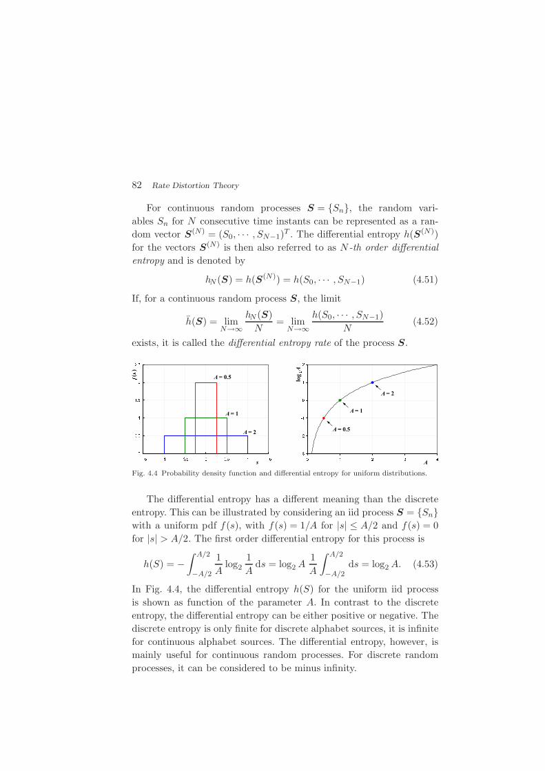
82 Rate Distortion Theory
For continuous random processes S = {Sn}, the random vari-
ables Sn for N consecutive time instants can be represented as a ran-
dom vector S(N) = (S0, · · · , SN−1)T . The differential entropy h(S(N))
for the vectors S(N) is then also referred to as N -th order differential
entropy and is denoted by
hN (S) = h(S(N)) = h(S0, · · · , SN−1) (4.51)
If, for a continuous random process S, the limit
h(S) = limN→∞
hN (S)
N= lim
N→∞h(S0, · · · , SN−1)
N(4.52)
exists, it is called the differential entropy rate of the process S.
Fig. 4.4 Probability density function and differential entropy for uniform distributions.
The differential entropy has a different meaning than the discrete
entropy. This can be illustrated by considering an iid process S = {Sn}with a uniform pdf f(s), with f(s) = 1/A for |s| ≤ A/2 and f(s) = 0
for |s| > A/2. The first order differential entropy for this process is
h(S) = −∫ A/2
−A/2
1
Alog2
1
Ads = log2 A
1
A
∫ A/2
−A/2ds = log2 A. (4.53)
In Fig. 4.4, the differential entropy h(S) for the uniform iid process
is shown as function of the parameter A. In contrast to the discrete
entropy, the differential entropy can be either positive or negative. The
discrete entropy is only finite for discrete alphabet sources, it is infinite
for continuous alphabet sources. The differential entropy, however, is
mainly useful for continuous random processes. For discrete random
processes, it can be considered to be minus infinity.

4.3. The Shannon Lower Bound 83
As an example, we consider a stationary Gaussian random process
with a mean µ and an N -th order autocovariance matrix CN . The N -th
order pdf fG(s) is given in (2.51), where µN represents a vector with all
N elements being equal to the mean µ. For the N -th order differential
entropy h(G)N of the stationary Gaussian process, we obtain
h(G)N (S) = −
∫
RN
fG(s) log2 fG(s) ds
=1
2log2
((2π)N |CN |
)
+1
2 ln 2
∫
RN
fG(s) (s−µN )T C−1N (s−µN ) ds. (4.54)
By reformulating the matrix multiplication in the last integral as sum,
it can be shown that for any random process with an N -th order pdf
f(s) and an N -th order autocovariance matrix CN ,∫
RN
f(s)(s − µN )T C−1N (s−µN ) ds = N. (4.55)
A step-by-step derivation of this result can be found in [11]. Inserting
(4.55) into (4.54) and using log2 e = (ln 2)−1 yields
h(G)N (S) =
1
2log2
((2π)N |CN |
)+
N
2log2 e
=1
2log2
((2πe)N |CN |
). (4.56)
Now, we consider any stationary random process S with a mean µ
and an N -th order autocovariance matrix CN . The N -th order pdf of
this process is denoted by f(s). Using the divergence inequality (4.21),
we obtain for its N -th order differential entropy,
hN (S) = −∫
RN
f(s) log2 f(s) ds
≤ −∫
RN
f(s) log2 fG(s) ds
=1
2log2
((2π)N |CN |
)
+1
2 ln 2
∫
RN
f(s)(s−µN )T C−1N (s−µN ) ds, (4.57)
84 Rate Distortion Theory
where fG(s) represents the N -th order pdf of the stationary Gaussian
process with the same mean µ and the same N -th order autocovariance
matrix CN . Inserting (4.55) and (4.56) yields
hN (S) ≤ h(G)N (S) =
1
2log2
((2πe)N |CN |
). (4.58)
Hence, the N -th order differential entropy of any stationary non-
Gaussian process is less than the N -th order differential entropy of a
stationary Gaussian process with the same N -th order autocovariance
matrix CN .
As shown in (4.56), the N -th order differential entropy of a station-
ary Gaussian process depends on the determinant of its N -th order
autocovariance matrix |CN |. The determinant |CN | is given by the
product of the eigenvalues ξi of the matrix CN , |CN | =∏N−1
i=0 ξi. The
trace of the N -th order autocovariance matrix tr(CN ) is given by the
sum of its eigenvalues, tr(CN ) =∑N−1
i=0 ξi, and, according to (2.39),
also by tr(CN ) = N · σ2, with σ2 being the variance of the Gaussian
process. Hence, for a given variance σ2, the sum of the eigenvalues is
constant. With the inequality of arithmetic and geometric means,
(N−1∏
i=0
xi
)1N
≤ 1
N
N−1∑
i=0
xi, (4.59)
which holds with equality if and only if x0 =x1 = . . .=xN−1, we obtain
the inequality
|CN | =N−1∏
i=0
ξi ≤(
1
N
N−1∑
i=0
ξi
)N
= σ2N . (4.60)
Equality holds if and only if all eigenvalues of CN are the same, i.e, if
and only if the Gaussian process is iid. Consequently, the N -th order
differential entropy of a stationary process S with a variance σ2 is
bounded by
hN (S) ≤ N
2log2
(2πeσ2
). (4.61)
It is maximized if and only if the process is a Gaussian iid process.

4.3. The Shannon Lower Bound 85
4.3.2 Shannon Lower Bound
Using the relationship (4.47) and the notation IN (gN ) = IN (S;S′), the
rate distortion function R(D) defined in (4.37) can be written as
R(D) = limN→∞
infgN : δN (gN )≤D
IN (S;S′)
N
= limN→∞
infgN : δN (gN )≤D
hN (S)− hN (S|S′)
N
= limN→∞
hN (S)
N− lim
N→∞sup
gN : δN (gN )≤D
hN (S|S′)
N
= h(S)− limN→∞
supgN : δN (gN )≤D
hN (S − S′|S′)
N, (4.62)
where the subscripts N indicate the N -th order mutual information
and differential entropy. The last equality follows from the fact that
the differential entropy is independent of the mean of a given pdf.
Since conditioning reduces the differential entropy, as has been
shown in (4.50), the rate distortion function is bounded by
R(D) ≥ RL(D), (4.63)
with
RL(D) = h(S)− limN→∞
supgN : δN (gN )≤D
hN (S − S′)
N. (4.64)
The lower bound RL(D) is called the Shannon lower bound (SLB).
For stationary processes and the MSE distortion measure, the dis-
tortion δN (gN ) in (4.64) is equal to the variance σ2Z of the process
Z = S − S′. Furthermore, we have shown in (4.61) that the maxi-
mum N -th order differential entropy for a stationary process with a
given variance σ2Z is equal to N
2 log2(2πeσ2Z). Hence, the Shannon lower
bound for stationary processes and MSE distortion is given by
RL(D) = h(S)− 1
2log2
(2πeD
). (4.65)
Since we concentrate on the MSE distortion measure in this text, we
call RL(D) given in (4.65) the Shannon lower bound in the following
without mentioning that it is only valid for the MSE distortion measure.
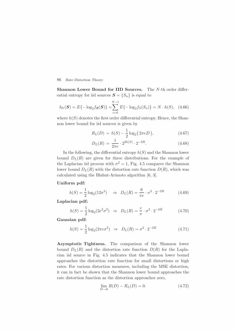
86 Rate Distortion Theory
Shannon Lower Bound for IID Sources. The N -th order differ-
ential entropy for iid sources S = {Sn} is equal to
hN (S) = E{− log2fS(S)} =
N−1∑
i=0
E{− log2fS(Sn)} = N · h(S), (4.66)
where h(S) denotes the first order differential entropy. Hence, the Shan-
non lower bound for iid sources is given by
RL(D) = h(S)− 1
2log2
(2πeD
), (4.67)
DL(R) =1
2πe· 22h(S) · 2−2R. (4.68)
In the following, the differential entropy h(S) and the Shannon lower
bound DL(R) are given for three distributions. For the example of
the Laplacian iid process with σ2 = 1, Fig. 4.5 compares the Shannon
lower bound DL(R) with the distortion rate function D(R), which was
calculated using the Blahut-Arimoto algorithm [6, 3].
Uniform pdf:
h(S) =1
2log2(12σ
2) ⇒ DL(R) =6
πe· σ2 · 2−2R (4.69)
Laplacian pdf:
h(S) =1
2log2(2e
2σ2) ⇒ DL(R) =e
π· σ2 · 2−2R (4.70)
Gaussian pdf:
h(S) =1
2log2(2πeσ2) ⇒ DL(R) = σ2 · 2−2R (4.71)
Asymptotic Tightness. The comparison of the Shannon lower
bound DL(R) and the distortion rate function D(R) for the Lapla-
cian iid source in Fig. 4.5 indicates that the Shannon lower bound
approaches the distortion rate function for small distortions or high
rates. For various distortion measures, including the MSE distortion,
it can in fact be shown that the Shannon lower bound approaches the
rate distortion function as the distortion approaches zero,
limD→0
R(D)−RL(D) = 0. (4.72)

4.3. The Shannon Lower Bound 87
Fig. 4.5 Comparison of the Shannon lower bound DL(R) and the distortion rate functionD(R) for a Laplacian iid source with unit variance (σ2 = 1).
Consequently, the Shannon lower bound represents a suitable reference
for the evaluation of lossy coding techniques at high rates or small
distortions. Proofs for the asymptotic tightness of the Shannon lower
bound for various distortion measures can be found in [48, 5, 47].
Shannon Lower Bound for Gaussian Sources. For sources with
memory, an exact analytic derivation of the Shannon lower bound is
usually not possible. One of the few examples for which the Shannon
lower bound can be expressed analytically is the stationary Gaussian
process. The N -th order differential entropy for a stationary Gaussian
process has been derived in (4.56). Inserting this result into the defini-
tion of the Shannon lower bound (4.65) yields
RL(D) = limN→∞
1
2Nlog2 |CN | −
1
2log2 D, (4.73)
where CN is the N -th order autocorrelation matrix. The determinant
of a matrix is given by the product of its eigenvalues. With ξ(N)i , for
i = 0, 1, . . . , N− 1, denoting the N eigenvalues of the N -th order auto-
correlation matrix CN , we obtain
RL(D) = limN→∞
1
2N
N−1∑
i=0
log2 ξ(N)i − 1
2log2 D. (4.74)
In order to proceed, we restrict our considerations to Gaussian pro-
cesses with zero mean, in which case the autocovariance matrix CN is

88 Rate Distortion Theory
equal to the autocorrelation matrix RN , and apply Grenander and
Szego’s theorem [29] for sequences of Toeplitz matrices. For a review
of Toeplitz matrices, including the theorem for sequences of Toeplitz
matrices, we recommend the tutorial [23]. Grenander and Szego’s
theorem can be stated as follows:
If RN is a sequence of Hermitian Toeplitz matrices
with elements φk on the k-th diagonal, the infimum
Φinf = infω Φ(ω) and supremum Φsup = supω Φ(ω) of
the Fourier series
Φ(ω) =∞∑
k=−∞φk e−jωk (4.75)
are finite, and the function G is continuous in the inter-
val [Φinf ,Φsup], then
limN→∞
1
N
N−1∑
i=0
G(
ξ(N)i
)
=1
2π
∫ π
−πG (Φ(ω)) dω, (4.76)
where ξ(N)i , for i = 0, 1, . . . , N − 1, denote the eigenval-
ues of the N -th matrix RN .
A matrix is called Hermitian if it is equal to its conjugate trans-
pose. This property is always fulfilled for real symmetric matrices as
the autocorrelation matrices of stationary processes. Furthermore, the
Fourier series (4.75) for the elements of the autocorrelation matrix RN
is the power spectral density ΦSS(ω). If we assume that the power spec-
tral density is finite and greater than 0 for all frequencies ω, the limit in
(4.74) can be replaced by an integral according to (4.76). The Shannon
lower bound RL(D) of a stationary Gaussian process with zero-mean
and a power spectral density ΦSS(ω) is given by
RL(D) =1
4π
∫ π
−πlog2
ΦSS(ω)
Ddω. (4.77)
A nonzero mean does not have any impact on the Shannon lower
bound RL(D), but on the power spectral density ΦSS(ω).

4.4. Rate Distortion Function for Gaussian Sources 89
For a stationary zero-mean Gauss-Markov process, the entries of the
autocorrelation matrix are given by φk = σ2ρ|k|, where σ2 is the signal
variance and ρ is the correlation coefficient between successive samples.
Using the relationship∑∞
k=1 ak e−jkx = a/(e−jx − a), we obtain
ΦSS(ω) =
∞∑
k=−∞σ2 ρ|k| e−jωk = σ2
(
1 +ρ
e−jω − ρ+
ρ
ejω − ρ
)
= σ2 1− ρ2
1− 2ρ cos ω + ρ2. (4.78)
Inserting this relationship into (4.77) yields
RL(D) =1
4π
∫ π
−πlog2
σ2(1− ρ2)
Ddω − 1
4π
∫ π
−πlog2(1− 2ρ cos ω + ρ2) dω
︸ ︷︷ ︸
=0
=1
2log2
σ2 (1− ρ2)
D, (4.79)
where we used∫ π0 ln(a2− 2ab cos x+ b2) dx = 2π ln a, for a ≥ b > 0. As
discussed above, the mean of a stationary process does not have any
impact on the Shannon rate distortion function or the Shannon lower
bound. Hence, the distortion rate function DL(R) for the Shannon
lower bound of a stationary Gauss-Markov process with a variance σ2
and a correlation coefficient ρ is given by
DL(R) = (1− ρ2)σ2 2−2R. (4.80)
This result can also be obtained by directly inserting the formula (2.50)
for the determinant |CN | of the N -th order autocovariance matrix for
Gauss-Markov processes into the expression (4.73).
4.4 Rate Distortion Function for Gaussian Sources
Stationary Gaussian sources play a fundamental role in rate distortion
theory. We have shown that the Gaussian source maximize the differ-
ential entropy, and thus also the Shannon lower bound, for a given
variance or autocovariance function. Stationary Gaussian sources are
also one of the few examples, for which the rate distortion function can
be exactly derived.

90 Rate Distortion Theory
4.4.1 Gaussian IID Sources
Before stating another important property of Gaussian iid sources, we
calculate their rate distortion function. Therefore, we first derive a
lower bound and then show that this lower bound is achievable. To
prove that the lower bound is achievable, it is sufficient to show that
there is a conditional pdf gS′|S(s′|s) for which the mutual information
I1(gS′|S) is equal to the lower bound for a given distortion D.
The Shannon lower bound for Gaussian iid sources as distortion
rate function DL(R) has been derived in sec. 4.3. The corresponding
rate distortion function is given by
RL(D) =1
2log2
σ2
D, (4.81)
where σ2 is the signal variance. For proving that the rate distortion
function is achievable, it is more convenient to look at the pdf of the
reconstruction fS′(s′) and the conditional pdf gS|S′(s|s′) of the input
given the reconstruction.
For distortions D < σ2, we choose
fS′(s′) =1
√
2π(σ2 −D)e− (s′−µ)2
2 (σ2−D) , (4.82)
gS|S′(s|s′) =1√2πD
e−(s−s′)2
2 D , (4.83)
where µ denotes the mean of the Gaussian iid process. It should be
noted that the conditional pdf gS|S′ represents a Gaussian pdf for the
random variables Zn = Sn − S′n, which are given by the difference of
the corresponding random variables Sn and S′n. We now verify that the
pdf fS(s) that we obtain with the choices (4.82) and (4.83) represents
the Gaussian pdf with a mean µ and a variance σ2. Since the random
variables Sn can be represented as the sum S′n + Zn, the pdf fS(s) is
given by the convolution of fS′(s′) and gS|S′(s|s′). And since means and
variances add when normal densities are convolved, the pdf fS(s) that
is obtained is a Gaussian pdf with a mean µ = µ + 0 and a variance
σ2 = (σ2−D) + D. Hence, the choices (4.82) and (4.83) are valid, and
4.4. Rate Distortion Function for Gaussian Sources 91
the conditional pdf gS′|S(s′|s) could be calculated using Bayes rule
gS′|S(s′|s) = gS|S′(s|s′) fS′(s′)fS(s)
. (4.84)
The resulting distortion is given by the variance of the difference process
Zn = Sn − S′n,
δ1(gS′|S) = E{(Sn − S′
n)2}
= E{Z2
n
}= D. (4.85)
For the mutual information, we obtain
I1(gS′|S) = h(Sn)− h(Sn|S′n) = h(Sn)− h(Sn − S′
n)
=1
2log2
(2πeσ2
)− 1
2log2
(2πeD
)=
1
2log2
σ2
D. (4.86)
Here, we used the fact that the conditional pdf gS|S′(s|s′) only depends
on the difference s− s′ as given by the choice (4.83).
The results show that, for any distortion D < σ2, we can find a con-
ditional pdf gS′|S that achieves the Shannon lower bound. For greater
distortions, we choose gS′|S(s′|s) = δ(0), which gives a distortion of σ2
and a rate of zero. Consequently, the rate distortion function for Gaus-
sian iid sources is given by
R(D) =
{12 log2
σ2
D : D < σ2
0 : D ≥ σ2 . (4.87)
The corresponding distortion rate function is given by
D(R) = σ2 2−2R. (4.88)
It is important to note that the rate distortion function for a Gaus-
sian iid process is equal to the Shannon lower bound for the entire
range of rates. Furthermore, it can be shown [4] that for every iid pro-
cess with a given variance σ2, the rate distortion function lies below
that of the Gaussian iid process with the same variance.
4.4.2 Gaussian Sources with Memory
For deriving the rate distortion function R(D) for a stationary Gaus-
sian process with memory, we decompose it into a number N of inde-
pendent stationary Gaussian sources. The N -th order rate distortion
92 Rate Distortion Theory
function RN (D) can then be expressed using the rate distortion func-
tion for Gaussian iid processes and the rate distortion function R(D)
is obtained by considering the limit of RN (D) as N approaches infinity.
As we stated in sec. 2.3, the N -th order pdf of a stationary Gaussian
process is given by
fS(s) =1
(2π)N/2 |CN |1/2e−
12(s−µN )T C−1
N (s−µN ) (4.89)
where s is a vector of N consecutive samples, µN is a vector with all
N elements being equal to the mean µ, and CN is the N -th order
autocovariance matrix. Since CN is a symmetric and real matrix, it
has N real eigenvalues ξ(N)i , for i = 0, 1, . . . , N− 1. The eigenvalues are
solutions of the equation
CN · v(N)i = ξ
(N)i · v(N)
i , (4.90)
where v(N)i represents a nonzero vector with unit norm, which is called a
unit-norm eigenvector corresponding to the eigenvalue ξ(N)i . Let AN be
the matrix whose columns are build by the N unit-norm eigenvectors,
AN =(
v(N)0 ,v
(N)1 , · · · ,v(N)
N−1
)
. (4.91)
By combining the N equations (4.90) for i = 0, 1, . . . , N − 1, we obtain
the matrix equation
CN AN = AN ΞN , (4.92)
where
ΞN =
ξ(N)0 0 . . . 0
0 ξ(N)1 . . . 0
......
. . . 0
0 0 0 ξ(N)N−1
(4.93)
is a diagonal matrix that contains the N eigenvalues of CN on its main
diagonal. The eigenvectors are orthogonal to each other and AN is an
orthogonal matrix.
Given the stationary Gaussian source {Sn}, we construct a source
{Un} by decomposing the source {Sn} into vectors S of N successive
random variables and applying the transform
U = A−1N (S − µN ) = AT
N (S − µN ) (4.94)

4.4. Rate Distortion Function for Gaussian Sources 93
to each of these vectors. Since AN is orthogonal, its inverse A−1 exists
and is equal to its transpose AT . The resulting source {Un} is given
by the concatenation of the random vectors U . Similarly, the inverse
transform for the reconstructions {U ′n} and {S′
n} is given by
S′ = AN U ′ + µN , (4.95)
with U ′ and S′ denoting the corresponding vectors of N successive
random variables. Since the coordinate mapping (4.95) is the inverse of
the mapping (4.94), the N -th order mutual information IN (U ;U ′) is
equal to the N -th order mutual information IN (S;S′). A proof of this
statement can be found in [4]. Furthermore, since AN is orthogonal,
the transform(U ′ −U
)= AN
(S′ − S
)(4.96)
preserves the Euclidean norm2. The MSE distortion between any real-
ization s of the random vector S and its reconstruction s′
dN (s; s′) =1
N
N−1∑
i=0
(si − s′i)2 =
1
N
N−1∑
i=0
(ui − u′i)
2 = dN (u;u′) (4.97)
is equal to the distortion between the corresponding vector u and its re-
construction u′. Hence, the N -th order rate distortion function RN (D)
for the stationary Gaussian source {Sn} is equal to the N -th order rate
distortion function for the random process {Un}.A linear transformation of a Gaussian random vector results in an-
other Gaussian random vector. For the mean vector and the autocor-
relation matrix of U , we obtain
E{U} = ATN (E{S} −µN ) = AT
N (µN − µN ) = 0 (4.98)
and
E{U UT
}= AT
N E{
(S − µN ) (S − µN )T}
AN
= ATN CN AN = ΞN . (4.99)
2 We will show in sec. 7.2 that every orthogonal transform preserves the MSE distortion.

94 Rate Distortion Theory
Since ΞN is a diagonal matrix, the pdf of the random vectors U is given
by the product
fU(u) =1
(2π)N/2 |ΞN |1/2e−
12uTΞ−1
N u =
N−1∏
i=0
1√
2πξ(N)i
e− u2
i
2 ξ(N)i
(4.100)
of the pdf’s of the Gaussian components Ui. Consequently, the compo-
nents Ui are independent of each other.
In sec. 4.2.2, we have shown how the N -th order mutual information
and the N -th order distortion for a code Q can be described by a con-
ditional pdf gQN = gU′ |U that characterizes the mapping of the random
vectors U onto the corresponding reconstruction vectors U ′. Due to the
independence of the components Ui of the random vectors U , the N -th
order mutual information IN (gQN ) and the N -th order distortion δN (gQ
N )
for a code Q can be written as
IN (gQN ) =
N−1∑
i=0
I1(gQi ) and δN (gQ
N ) =1
N
N−1∑
i=0
δ1(gQi ), (4.101)
where gQi = gU ′
i |Uispecifies the conditional pdf for the mapping of a
vector component Ui onto its reconstruction U ′i . Consequently, the N -th
order distortion rate function DN (R) can be expressed by
DN (R) =1
N
N−1∑
i=0
Di(Ri) with R =1
N
N−1∑
i=0
Ri, (4.102)
where Ri(Di) denotes the first order rate distortion function for a vector
component Ui. The first order distortion rate function for Gaussian
sources has been derived in sec. 4.4.1 and is given by
Di(Ri) = σ2i 2−2Ri . (4.103)
The variances σ2i of the vector component Ui are equal to the eigenval-
ues ξ(N)i of the N -th order autocovariance matrix CN . Hence, the N -th
order distortion rate function can be written as
DN (R) =1
N
N−1∑
i=0
ξ(N)i 2−2Ri with R =
1
N
N−1∑
i=0
Ri. (4.104)

4.4. Rate Distortion Function for Gaussian Sources 95
With the inequality of arithmetic and geometric means, which holds
with equality if and only if all elements have the same value, we obtain
DN (R) ≥(
N−1∏
i=0
ξ(N)i 2−2Ri
) 1N
=
(N−1∏
i=0
ξ(N)i
) 1N
· 2−2R = ξ(N) · 2−2R,
(4.105)
where ξ(N) denotes the geometric mean of the eigenvalues ξ(N)i . For a
given N -th order mutual information R, the distortion is minimized
if and only if ξ(N)i 2−2Ri is equal to ξ(N)2−2R for all i = 0, · · · , N − 1,
which yields
Ri = R +1
2log2
ξ(N)i
ξ(N). (4.106)
In the above result, we have ignored the fact that the mutual in-
formation Ri for a component Ui cannot be less than zero. Since the
distortion rate function given in (4.103) is steeper at low Ri, the mutual
information Ri for components with ξ(N)i < ξ(N)2−2R has to be set equal
to zero and the mutual information R has to be distributed among the
remaining components in order to minimize the distortion. This can
be elegantly specified by introducing a parameter θ, with θ ≥ 0, and
setting the component distortions according to
Di = min(
θ, ξ(N)i
)
. (4.107)
This concept is also know as inverse water-filling for independent Gaus-
sian sources [57], where the parameter θ can be interpreted as the water
level. Using (4.103), we obtain for the mutual information Ri,
Ri =1
2log2
ξ(N)i
min(
θ, ξ(N)i
) = max
(
0,1
2log2
ξ(N)i
θ
)
. (4.108)
The N -th order rate distortion function RN (D) can be expressed by
the following parametric formulation, with θ ≥ 0,
DN (θ) =1
N
N−1∑
i=0
Di =1
N
N−1∑
i=0
min(
θ, ξ(N)i
)
, (4.109)
RN (θ) =1
N
N−1∑
i=0
Ri =1
N
N−1∑
i=0
max
(
0,1
2log2
ξ(N)i
θ
)
. (4.110)
96 Rate Distortion Theory
The rate distortion function R(D) for the stationary Gaussian ran-
dom process {Sn} is given by the limit
R(D) = limN→∞
RN (D), (4.111)
which yields the parametric formulation, with θ > 0,
D(θ) = limN→∞
DN (θ), R(θ) = limN→∞
RN (θ). (4.112)
For Gaussian processes with zero mean (CN = RN ), we can apply the
theorem for sequences of Toeplitz matrices (4.76) to express the rate
distortion function using the power spectral density ΦSS(ω) of the
source. A parametric formulation, with θ ≥ 0, for the rate distortion
function R(D) for a stationary Gaussian source with zero mean and a
power spectral density ΦSS(ω) is given by
D(θ) =1
2π
∫ π
−πmin (θ, ΦSS(ω)) dω, (4.113)
R(θ) =1
2π
∫ π
−πmax
(
0,1
2log2
ΦSS(ω)
θ
)
dω. (4.114)
The minimization in the parametric formulation (4.113) and (4.114)
of the rate distortion function is illustrated in Fig. 4.6. It can be in-
terpreted that at each frequency, the variance of the corresponding
frequency component as given by the power spectral density ΦSS(ω) is
compared to the parameter θ, which represents the mean squared error
of the frequency component. If ΦSS(ω) is found to be larger than θ,
the mutual information is set equal to 12 log2
ΦSS(ω)θ , otherwise a mutual
information of zero is assigned to that frequency component.
For stationary zero-mean Gauss-Markov sources with a variance σ2
and a correlation coefficient ρ, the power spectral density ΦSS(ω) is
given by (4.78). If we choose the parameter θ according to
θ ≥ min∀ω
ΦSS(ω) = σ2 1− ρ2
1− 2ρ + ρ2= σ2 1− ρ
1 + ρ, (4.115)
we obtain the parametric equations
D(θ) =1
2π
∫ π
−πθ dω = θ, (4.116)
R(θ) =1
4π
∫ π
−πlog2
ΦSS(ω)
θdω =
1
2log2
σ2 (1− ρ2)
θ, (4.117)
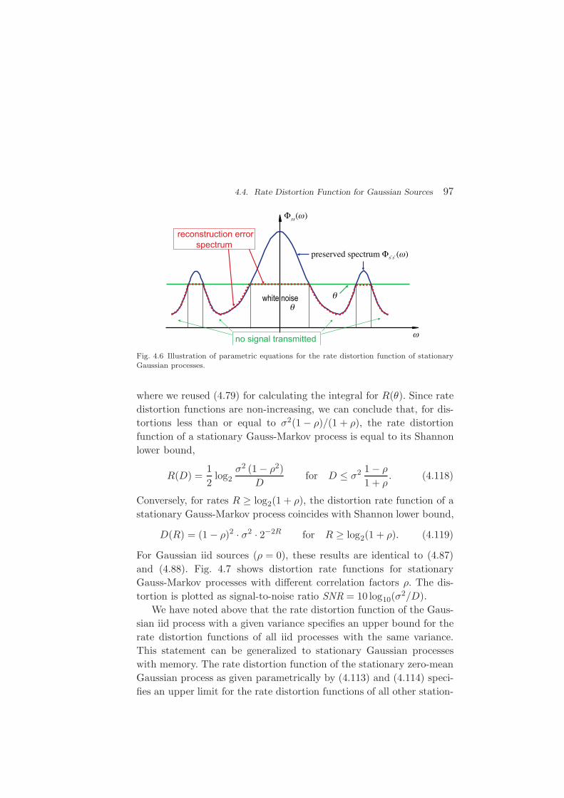
4.4. Rate Distortion Function for Gaussian Sources 97
white noise
reconstruction error
spectrum
no signal transmitted
"ss(#)
"
!
preserved spectrum " # s # s ($)
"
Fig. 4.6 Illustration of parametric equations for the rate distortion function of stationaryGaussian processes.
where we reused (4.79) for calculating the integral for R(θ). Since rate
distortion functions are non-increasing, we can conclude that, for dis-
tortions less than or equal to σ2(1− ρ)/(1 + ρ), the rate distortion
function of a stationary Gauss-Markov process is equal to its Shannon
lower bound,
R(D) =1
2log2
σ2 (1− ρ2)
Dfor D ≤ σ2 1− ρ
1 + ρ. (4.118)
Conversely, for rates R ≥ log2(1 + ρ), the distortion rate function of a
stationary Gauss-Markov process coincides with Shannon lower bound,
D(R) = (1− ρ)2 · σ2 · 2−2R for R ≥ log2(1 + ρ). (4.119)
For Gaussian iid sources (ρ = 0), these results are identical to (4.87)
and (4.88). Fig. 4.7 shows distortion rate functions for stationary
Gauss-Markov processes with different correlation factors ρ. The dis-
tortion is plotted as signal-to-noise ratio SNR = 10 log10(σ2/D).
We have noted above that the rate distortion function of the Gaus-
sian iid process with a given variance specifies an upper bound for the
rate distortion functions of all iid processes with the same variance.
This statement can be generalized to stationary Gaussian processes
with memory. The rate distortion function of the stationary zero-mean
Gaussian process as given parametrically by (4.113) and (4.114) speci-
fies an upper limit for the rate distortion functions of all other station-

98 Rate Distortion Theory
R [bits]!
0! 0.5! 1! 1.5! 2! 2.5! 3! 3.5! 40!
5!
10!
15!
20!
25!
30!
35!
40!
45!!"=0.99!
!"=0.95!!"=0.9!!"=0.78!!"=0.5!!"=0!
SNR [dB]
D*
" 2#1$ %
1+ %
Fig. 4.7 Distortion rate functions for Gauss-Markov processes with different correlationfactors ρ. The distortion D is plotted as signal-to-noise ratio SNR = 10 log10(σ2/D).
ary processes with the same power spectral density ΦSS(ω). A proof of
this statement can be found in [4].
4.5 Summary of Rate Distortion Theory
Rate distortion theory addresses the problem of finding the greatest
lower bound for the average number of bits that is required for repre-
senting a signal without exceeding a given distortion. We introduced
the operational rate distortion function that specifies this fundamental
bound as infimum of over all source codes. A fundamental result of
rate distortion theory is that the operational rate distortion function
is equal to the information rate distortion function, which is defined as
infimum over all conditional pdf’s for the reconstructed samples given
the original samples. Due to this equality, both the operational and
the information rate distortion function are usually referred to as the
rate distortion function. It has further been noted that, for the MSE
distortion measure, the lossless coding theorem specifying that the av-
erage codeword length per symbol cannot be less than the entropy rate
represents a special case of rate distortion theory for discrete sources
with zero distortion.
For most sources and distortion measures, it is not known how to

4.5. Summary of Rate Distortion Theory 99
analytically derive the rate distortion function. A useful lower bound
for the rate distortion function is given by the so-called Shannon lower
bound. The difference between the Shannon lower bound and the rate
distortion function approaches zero as the distortion approaches zero or
the rate approaches infinity. Due to this property, it represents a suit-
able reference for evaluating the performance of lossy coding schemes
at high rates. For the MSE distortion measure, an analytical expression
for the Shannon lower bound can be given for typical iid sources as well
as for general stationary Gaussian sources.
An important class of processes is the class of stationary Gaussian
processes. For Gaussian iid processes and MSE distortion, the rate dis-
tortion function coincides with the Shannon lower bound for all rates.
The rate distortion function for general stationary Gaussian sources
with zero mean and MSE distortion can be specified as a paramet-
ric expression using the power spectral density. It has also been noted
that the rate distortion function of the stationary Gaussian process
with zero mean and a particular power spectral density represents an
upper bound for all stationary processes with the same power spectral
density, which leads to the conclusion that Gaussian sources are the
most difficult to code.

5
Quantization
Lossy source coding systems, which we have introduced in chapter 4,
are characterized by the fact that the reconstructed signal is not identi-
cal to the source signal. The process that introduces the corresponding
loss of information (or signal fidelity) is called quantization. An appara-
tus or algorithmic specification that performs the quantization process
is referred to as quantizer. Each lossy source coding system includes
a quantizer. The rate distortion point associated with a lossy source
coding system is to a wide extent determined by the used quantization
process. For this reason, the analysis of quantization techniques is of
fundamental interest for the design of source coding systems.
In this chapter, we analyze the quantizer design and the perfor-
mance of various quantization techniques with the emphasis on scalar
quantization, since it is the most widely used quantization technique in
video coding. To illustrated the inherent limitation of scalar quantiza-
tion, we will also briefly introduce the concept of vector quantization
and show its advantage with respect to the achievable rate distortion
performance. For further details, the reader is referred to the com-
prehensive treatment of quantization in [16] and the overview of the
history and theory of quantization in [28].
100

5.1. Structure and Performance of Quantizers 101
5.1 Structure and Performance of Quantizers
In the broadest sense, quantization is an irreversible deterministic map-
ping of an input quantity to an output quantity. For all cases of prac-
tical interest, the set of obtainable values for the output quantity is
finite and includes fewer elements than the set of possible values for
the input quantity. If the input quantity and the output quantity are
scalars, the process of quantization is referred to as scalar quantiza-
tion. A very simple variant of scalar quantization is the rounding of a
real input value to its nearest integer value. Scalar quantization is by
far the most popular form of quantization and is used in virtually all
video coding applications. However, as we will see later, there is a gap
between the operational rate distortion curve for optimal scalar quan-
tizers and the fundamental rate distortion bound. This gap can only
be reduced if a vector of more than one input sample is mapped to
a corresponding vector of output samples. In this case, the input and
output quantity are vectors and the quantization process is referred to
as vector quantization. Vector quantization can asymptotically achieve
the fundamental rate distortion bound if the number of samples in the
input and output vector approaches infinity.
A quantizer Q of dimension N specifies a mapping of the
N -dimensional Euclidean space RN into a finite1 set of reconstruction
vectors inside the N -dimensional Euclidean space RN,
Q : RN → {s′
0, s′
1, · · · , s′
K−1} . (5.1)
If the dimension N of the quantizer Q is equal to 1, it is a scalar
quantizer; otherwise, it is a vector quantizer. The number K of recon-
struction vectors is also referred to as the size of the quantizer Q. The
deterministic mapping Q associates a subset Ci of the N -dimensional
Euclidean space RN with each of the reconstruction vectors s′
i. The
subsets Ci, with 0 ≤ i < K, are called quantization cells and are de-
fined by
Ci ={s ∈ RN : Q(s) = s′
i
}. (5.2)
1 Although we restrict our considerations to finite sets of reconstruction vectors, some ofthe presented quantization methods and derivations are also valid for countably infinitesets of reconstruction vectors.

102 Quantization
From this definition, it follows that the quantization cells Ci form a
partition of the N -dimensional Euclidean space RN ,
K−1⋃
i=0
Ci = RN with ∀i 6= j : Ci ∩ Cj = ∅. (5.3)
Given the quantization cells Ci and the associated reconstruction val-
ues s′
i, the quantization mapping Q can be specified by
Q(s) = s′
i ∀s ∈ Ci. (5.4)
A quantizer is completely specified by the set of reconstruction values
and the associated quantization cells.
For analyzing the design and performance of quantizers, we consider
the quantization of symbol sequences {sn} that represent realizations
of a random process {Sn}. For the case of vector quantization (N > 1),
the samples of the input sequence {sn} shall be arranged in vectors,
resulting in a sequence of symbol vectors {sn}. Usually, the input se-
quence {sn} is decomposed into blocks of N samples and the compo-
nents of an input vector sn are build be the samples of such a block,
but other arrangements are also possible. In any case, the sequence of
input vectors {sn} can be considered to represent a realization of a
vector random process {Sn}. It should be noted that the domain of
the input vectors sn can be a subset of the N -dimensional space RN ,
which is the case if the random process {Sn} is discrete or its marginal
pdf f(s) is zero outside a finite interval. However, even in this case, we
can generally consider quantization as a mapping of the N -dimensional
Euclidean space RN into a finite set of reconstruction vectors.
Fig. 5.1 shows a block diagram of a quantizer Q. Each input vec-
tor sn is mapped onto one of the reconstruction vectors, given by Q(sn).
Fig. 5.1 Basic structure of a quantizer Q in combination with a lossless coding γ.
5.1. Structure and Performance of Quantizers 103
The average distortion D per sample between the input and out-
put vectors depends only on the statistical properties of the input
sequence {sn} and the quantization mapping Q. If the random pro-
cess {Sn} is stationary, it can be expressed by
D = E{dN (Sn, Q(Sn))} =1
N
K−1∑
i=0
∫
Ci
dN (s, Q(s)) fS(s) ds, (5.5)
where fS denotes the joint pdf of the vector components of the random
vectors Sn. For the MSE distortion measure, we obtain
D =1
N
K−1∑
i=0
∫
Ci
fS(s) (s − s′
i)T (s− s′
i) ds. (5.6)
Unlike the distortion D, the average transmission rate is not only
determined by the quantizer Q and the input process. As illustrated
in Fig. 5.1, we have to consider the lossless coding γ by which the
sequence of reconstruction vectors {Q(sn)} is mapped onto a sequence
of codewords. For calculating the performance of a quantizer or for
designing a quantizer we have to make reasonable assumptions about
the lossless coding γ. It is certainly not a good idea to assume a lossless
coding with an average codeword length per symbol close to the entropy
for the design, but to use the quantizer in combination with fixed-length
codewords for the reconstruction vectors. Similarly, a quantizer that
has been optimized under the assumption of fixed-length codewords is
not optimal if it is used in combination with advanced lossless coding
techniques such as Huffman coding or arithmetic coding.
The rate R of a coding system consisting of a quantizer Q and a
lossless coding γ is defined as the average codeword length per input
sample. For stationary input processes {Sn}, it can be expressed by
R =1
NE{ |γ( Q(Sn) )| } =
1
N
N−1∑
i=0
p(s′
i) · |γ(s′
i)| , (5.7)
where |γ(s′
i)| denotes the average codeword length that is obtained for
a reconstruction vector s′
i with the lossless coding γ and p(s′
i) denotes
the pmf for the reconstruction vectors, which is given by
p(s′
i) =
∫
Ci
fS(s) ds. (5.8)

104 Quantization
Fig. 5.2 Lossy source coding system consisting of a quantizer, which is decomposed into anencoder mapping α and a decoder mapping β, and a lossless coder γ.
The probability of a reconstruction vector does not depend on the
reconstruction vector itself, but only on the associated quantization
cell Ci.A quantizer Q can be decomposed into two parts, an encoder map-
ping α which maps the input vectors sn to quantization indexes i, with
0 ≤ i < K, and a decoder mapping β which maps the quantization
indexes i to the associated reconstruction vectors s′
i. The quantizer
mapping can then be expressed by Q(s) = α(β(s)). The loss of signal
fidelity is introduced as a result of the encoder mapping α, the decoder
mapping β merely maps the quantization indexes i to the associated
reconstruction vectors s′
i. The combination of the encoder mapping α
and the lossless coding γ forms an encoder of a lossy source coding
system as illustrated in Fig. 5.2. The corresponding decoder is given
by the inverse lossless coding γ−1 and the decoder mapping β.
5.2 Scalar Quantization
In scalar quantization (N = 1), the input and output quantity are
scalars. Hence, a scalar quantizer Q of size K specifies a mapping of
the real line R into a set of K reconstruction levels,
Q : R → {s′0, s′1, · · · , s′K−1}. (5.9)
In the general case, a quantization cell Ci corresponds to a set of in-
tervals of the real line. We restrict our considerations to regular scalar
quantizers for which each quantization cell Ci represents a single in-
terval of the real line R and the reconstruction levels s′i are located
inside the associated quantization cells Ci. Without loss of generality,
we further assume that the quantization cells are ordered in increasing
order of the values of their lower interval boundary. When we further
assume that the quantization intervals include the lower, but not the

5.2. Scalar Quantization 105
Fig. 5.3 Input-output function Q of a scalar quantizer.
higher interval boundary, each quantization cell can be represented by
a half-open2 interval Ci = [ui, ui+1). The interval boundaries ui are also
referred to as decision thresholds. The interval sizes ∆i = ui+1 − ui are
called quantization step sizes. Since the quantization cells must form a
partition of the real line R, the values u0 and uK are fixed and given
by u0 = −∞ and uK =∞. Consequently, K reconstruction levels and
K−1 decision thresholds can be chosen in the quantizer design.
The quantizer mapping Q of a scalar quantizer as defined above
can be represented by a piecewise-constant input-output function as
illustrated in Fig. 5.3. All input values s with ui ≤ s < ui+1 are assigned
to the corresponding reproduction level s′i.In the following treatment of scalar quantization, we generally as-
sume that the input process is stationary. For continuous random pro-
cesses, scalar quantization can then can be interpreted as a discretiza-
tion of the marginal pdf f(s) as illustrated in Fig. 5.4.
For any stationary process {S} with a marginal pdf f(s), the quan-
tizer output is a discrete random process {S′} with a marginal pmf
p(s′i) =
∫ ui+1
ui
f(s) ds. (5.10)
2 In strict mathematical sense, the first quantization cell is an open interval C0 = (−∞, u1).
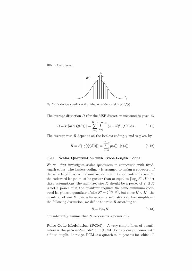
106 Quantization
Fig. 5.4 Scalar quantization as discretization of the marginal pdf f(s).
The average distortion D (for the MSE distortion measure) is given by
D = E{d(S,Q(S))} =
K−1∑
i=0
∫ ui+1
ui
(s− s′i)2 · f(s) ds. (5.11)
The average rate R depends on the lossless coding γ and is given by
R = E{|γ(Q(S))|} =
N−1∑
i=0
p(s′i) · |γ(s′i)|. (5.12)
5.2.1 Scalar Quantization with Fixed-Length Codes
We will first investigate scalar quantizers in connection with fixed-
length codes. The lossless coding γ is assumed to assign a codeword of
the same length to each reconstruction level. For a quantizer of size K,
the codeword length must be greater than or equal to ⌈log2 K⌉. Under
these assumptions, the quantizer size K should be a power of 2. If K
is not a power of 2, the quantizer requires the same minimum code-
word length as a quantizer of size K ′ = 2⌈log2 K⌉, but since K < K ′, the
quantizer of size K ′ can achieve a smaller distortion. For simplifying
the following discussion, we define the rate R according to
R = log2 K, (5.13)
but inherently assume that K represents a power of 2.
Pulse-Code-Modulation (PCM). A very simple form of quanti-
zation is the pulse-code-modulation (PCM) for random processes with
a finite amplitude range. PCM is a quantization process for which all
5.2. Scalar Quantization 107
quantization intervals have the same size ∆ and the reproduction val-
ues s′i are placed in the middle between the decision thresholds ui and
ui+1. For general input signals, this is not possible since it results in an
infinite number of quantization intervals K and hence an infinite rate
for our fixed-length code assumption. However, if the input random
process has a finite amplitude range of [smin, smax], the quantization
process is actually a mapping of the finite interval [smin, smax] to the
set of reproduction levels. Hence, we can set u0 = smin and uK = smax.
The width A = smax − smin of the amplitude interval is then evenly
split into K quantization intervals, resulting in a quantization step size
∆ =A
K= A · 2−R. (5.14)
The quantization mapping for PCM can be specified by
Q(s) =
⌊s− smin
∆+ 0.5
⌋
·∆ + smin. (5.15)
As an example, we consider PCM quantization of a stationary random
process with an uniform distribution, f(s) = 1A for −A
2 ≤ s ≤ A2 . The
distortion as defined in (5.11) becomes
D =
K−1∑
i=0
∫ smin+(i+1)∆
smin+i∆
1
A
(
s− smin −(
i +1
2
)
·∆)2
ds. (5.16)
By carrying out the integration and inserting (5.14), we obtain the
operational distortion rate function,
DPCM,uniform(R) =A2
12· 2−2R = σ2 · 2−2R. (5.17)
For stationary random processes with an infinite amplitude range,
we have to choose u0 = −∞ and uK =∞. The inner interval bound-
aries ui, with 0 < i < K, and the reconstruction levels s′i can be evenly
distributed around the mean value µ of the random variables S. For
symmetric distributions (µ = 0), this gives
s′i =
(
i− K − 1
2
)
·∆ for 0 ≤ i < K, (5.18)
ui =
(
i− K
2
)
·∆ for 0 < i < K. (5.19)

108 Quantization
1 2 3 40
5
10
15
20
25
R [bit/symbol]
SN
R [d
B]
Solid lines: Shannon Lower Bound
Dashed lines/circles: pdf−optimzed uniform quantization
UL
G
U: Uniform pdfL: Laplacian pdfG: Gaussian pdf
Solid lines: Shannon Lower Bound
Dashed lines/circles: pdf−optimzed uniform quantization
UL
G
U: Uniform pdfL: Laplacian pdfG: Gaussian pdf
Solid lines: Shannon Lower Bound
Dashed lines/circles: pdf−optimzed uniform quantization
UL
G
U: Uniform pdfL: Laplacian pdfG: Gaussian pdf
1 2 3 40
0.5
1
1.5
2
R [bit/symbol]
∆ opt/σ
U
L
G
U
L
G
U
L
G
Fig. 5.5 PCM quantization of stationary random processes with uniform (U), Laplacian (L),and Gaussian (G) distributions: (left) operational distortion rate functions in comparisonto the corresponding Shannon lower bounds (for variances σ2 = 1); (right) optimal quanti-zation step sizes.
Inserting these expressions into (5.11) yields an expression for the dis-
tortion D(∆) that depends only on the quantization step size ∆ for a
given quantizer size K. The quantization step size ∆ can be chosen in a
way that the distortion is minimized. As an example, we minimized the
distortions for the uniform, Laplacian, and Gaussian distribution for
given quantizer sizes K by numerical optimization. The obtained oper-
ational rate distortion curves and corresponding quantization step sizes
are depicted in Fig. 5.5. The numerically obtained results for the uni-
form distribution are consistent with (5.17) and (5.14). For the Lapla-
cian and Gaussian distribution, the loss in SNR with respect to the
Shannon lower bound (high-rate approximation of the distortion rate
function) is significant and increases toward higher rates.
Pdf-Optimized ScalarQuantizationwithFixed-LengthCodes.
For the application of PCM quantization to stationary random
processes with an infinite amplitude interval, we have chosen the
quantization step size for a given quantizer size K by minimizing
the distortion. A natural extension of this concept is to minimize
the distortion with respect to all parameters of a scalar quantizer of
a given size K. The optimization variables are the K − 1 decision
thresholds ui, with 0 < i < K, and the K reconstruction levels s′i, with

5.2. Scalar Quantization 109
0 ≤ i < K. The obtained quantizer is called a pdf-optimized scalar
quantizer with fixed-length codes.
For deriving a condition for the reconstruction levels s′i, we first
assume that the decision thresholds ui are given. The overall distor-
tion (5.11) is the sum of the distortions Di for the quantization inter-
vals Ci = [ui, uu+1). For given decision thresholds, the interval distor-
tions Di are mutually independent and are determined by the corre-
sponding reconstruction levels s′i,
Di(s′i) =
∫ ui+1
ui
d1(s, s′i) · f(s) ds. (5.20)
By using the conditional distribution f(s|s′i) = f(s) · p(s′i), we obtain
Di(s′i) =
1
p(s′i)
ui+1∫
ui
d1(s, s′i) · f(s|s′i) ds =
E{d1(S, s′i)|S∈ Ci}p(s′i)
. (5.21)
Since p(s′i) does not depend on s′i, the optimal reconstruction levels s′∗iare given by
s′∗i = arg mins′∈R
E{d1(S, s′)|S∈ Ci
}, (5.22)
which is also called the generalized centroid condition. For the squared
error distortion measure d1(s, s′) = (s− s′)2, the optimal reconstruc-
tion levels s′∗i are the conditional means (centroids)
s′∗i = E{S|S∈ Ci} =
∫ ui+1
uis · f(s) ds
∫ ui+1
uif(s) ds
. (5.23)
This can be easily proved by the inequality
E{(S − s′i)
2}
= E{(S −E{S}+ E{S} − s′i)
2}
= E{(S −E{S})2
}+ (E{S} − s′i)
2
≥ E{(S −E{S})2
}. (5.24)
If the reproduction levels s′i are given, the overall distortion D is
minimized if each input value s is mapped to the reproduction level s′ithat minimizes the corresponding sample distortion d1(s, s
′i),
Q(s) = arg min∀s′i
d1(s, s′i). (5.25)
110 Quantization
This condition is also referred to as the nearest neighbor condition.
Since a decision threshold ui influences only the distortions Di of the
neighboring intervals, the overall distortion is minimized if
d1(ui, s′i−1) = d1(ui, s
′i) (5.26)
holds for all decision thresholds ui, with 0 < i < K. For the squared
error distortion measure, the optimal decision thresholds u∗i , with
0 < i < K, are given by
u∗i =
1
2(s′i−1 + s′i). (5.27)
The expressions (5.23) and (5.27) can also be obtained by setting the
partial derivatives of the distortion (5.11) with respect to the decision
thresholds ui and the reconstruction levels s′i equal to zero [56].
The Lloyd Algorithm. The necessary conditions for the optimal
reconstruction levels (5.22) and decision thresholds (5.25) depend on
each other. A corresponding iterative algorithm for minimizing the dis-
tortion of a quantizer of given size K was suggested by Lloyd [49]
and is commonly called the Lloyd algorithm. The obtained quantizer
is referred to as Lloyd quantizer or Lloyd-Max3 quantizer. For a given
pdf f(s), first an initial set of unique reconstruction levels {s′i} is ar-
bitrarily chosen, then the decision thresholds {ui} and reconstruction
levels {s′i} are alternately determined according to (5.25) and (5.22),
respectively, until the algorithm converges. It should be noted that the
fulfillment of the conditions (5.22) and (5.25) is in general not sufficient
to guarantee the optimality of the quantizer. The conditions are only
sufficient if the pdf f(s) is log-concave. One of the examples, for which
the Lloyd algorithm yields a unique solution independent of the initial
set of reconstruction levels, is the Gaussian pdf.
Often, the marginal pdf f(s) of a random process is not known
a priori. In such a case, the Lloyd algorithm can be applied using a
training set. If the training set includes a sufficiently large number of
samples, the obtained quantizer is an accurate approximation of the
3 Lloyd and Max independently observed the two necessary conditions for optimality.

5.2. Scalar Quantization 111
Lloyd quantizer. Using the encoder mapping α (see sec. 5.1), the Lloyd
algorithm for a training set of samples {sn} and a given quantizer size K
can be stated as follows:
(1) Choose an initial set of unique reconstruction levels {s′i}.(2) Associate all samples of the training set {sn} with one of the
quantization intervals Ci according to
α(sn) = arg min∀i
d1(sn, s′i) (nearest neighbor condition)
and update the decision thresholds {ui} accordingly.
(3) Update the reconstruction levels {s′i} according to
s′i = arg mins′∈R
E{d1(S, s′) |α(S) = i
}, (centroid condition)
where the expectation value is taken over the training set.
(4) Repeat the previous two steps until convergence.
Examples for the Lloyd Algorithm. As a first example, we ap-
plied the Lloyd algorithm with a training set of more than 10000 sam-
ples and the MSE distortion measure to a Gaussian pdf with unit vari-
ance. We used two different initializations for the reconstruction levels.
Convergence was determined if the relative distortion reduction be-
tween two iterations steps was less than 1%, (Dk −Dk+1)/Dk+1 < 0.01.
The algorithm quickly converged after 6 iterations for both initializa-
tions to the same overall distortion D∗F . The obtained reconstruction
levels {s′i} and decision thresholds {ui} as well as the iteration processes
for the two initializations are illustrated in Fig. 5.6.
The same algorithm with the same two initializations was also ap-
plied to a Laplacian pdf with unit variance. Also for this distribution,
the algorithm quickly converged after 6 iterations for both initializa-
tions to the same overall distortion D∗F . The obtained quantizer and
the iteration processes are illustrated in Fig. 5.7.
5.2.2 Scalar Quantization with Variable-Length Codes
We have investigated the design of quantizers that minimize the distor-
tion for a given number K of reconstruction levels, which is equivalent

112 Quantization
Decision thresholds ui:
u1 = −0.98, u2 = 0, u3 = 0.98
Decoding symbols s′i:
s′0 = −1.51, s′1 = −0.45
s′2 = 0.45, s′3 = 1.51
Distortion: D∗F = 0.12 = 9.3 dB
−5 −4 −3 −2 −1 0 1 2 3 4 50
0.1
0.2
0.3
0.4
0.5
s
f( s
)
u1
u2
u3
s’0
s’1
s’2
s’3
Initialization A:s′i = −3.75 + 2.5 · i
0 1 2 3 4 5 6 7 8 9 10 11 12−5−4−3−2−1
012345
u3
u1
u2
u4
u0
∞
−∞
s’0
s’1
s’2
s’3
0 1 2 3 4 5 6 7 8 9 10 11 12−2
02468
1012141618
D
D0
D3
D1
D2
−10 log10
D
−10 log10
( Di K)
Initialization B:s′3/0 = +/− 1.15, s′2/1 = +/− 0.32
0 1 2 3 4 5 6 7 8 9 10 11 12−5−4−3−2−1
012345
u3
u1
u2
u4
u0
∞
−∞
s’0
s’1
s’2
s’3
0 1 2 3 4 5 6 7 8 9 10 11 12−2
02468
1012141618
DD
0D
3
D1D2
−10 log10
D
−10 log10
( Di K)
Fig. 5.6 Lloyd algorithm for a Gaussian pdf with unit variance and two initializations:(top) final reconstruction levels and decision thresholds; (middle) reconstruction levels anddecision thresholds as function of the iteration step; (bottom) overall SNR and SNR for thequantization intervals as function of the iteration step.
to a quantizer optimization using the assumption that all reconstruc-
tion levels are signaled with codewords of the same length. Now we con-
sider the quantizer design in combination with variable-length codes γ.
The average codeword length that is associated with a particular
reconstruction level s′i is denoted by ℓ(s′i) = |γ(s′i)|. If we use a scalar
Huffman code, ℓ(s′i) is equal to the length of the codeword that is

5.2. Scalar Quantization 113
Decision thresholds ui:
u1 = −1.13, u2 = 0, u3 = 1.13
Decoding symbols s′i:
s′0 = −1.83, s′1 = −0.42
s′2 = 0.42, s′3 = 1.83
Distortion: D∗F = 0.18 = 7.55 dB
−5 −4 −3 −2 −1 0 1 2 3 4 50
0.1
0.2
0.3
0.4
0.5
0.6
0.7
0.8
s
f( s
)
u1
u2
u3
s’0
s’1
s’2
s’3
Initialization A:s′i = −3.75 + 2.5 · i
! " # $ % & ' ( ) * "! "" "#!&
!%
!$
!#
!"
!
"
#
$
%
&
u$
u"
u#
u%
u!
!
!!
s+!
s+"
s+#
s+$
! " # $ % & ' ( ) * "! "" "#!#
!
#
%
'
)
"!
"#
"%
"'
+
+!
+$
+"+#
!"!,-./"!
D
!"!,-./"!0 D
i N1
Initialization B:s′3/0 = +/− 1.15, s′2/1 = +/− 0.32
! " # $ % & ' ( ) * "! "" "#!&
!%
!$
!#
!"
!
"
#
$
%
&
u$
u"
u#
u%
u!
!
!!
s+!
s+"
s+#
s+$
! " # $ % & ' ( ) * "! "" "#!#
!
#
%
'
)
"!
"#
"%
"'
+
+!
+$
+"+#
!"!,-./"!
D
!"!,-./"!0 D
i N1
Fig. 5.7 Lloyd algorithm for a Laplacian pdf with unit variance and two initializations:(top) final reconstruction levels and decision thresholds; (middle) reconstruction levels anddecision thresholds as function of the iteration step; (bottom) overall SNR and SNR for thequantization intervals as function of the iteration step.
assigned to s′i. According to (5.12), the average rate R is given by
R =
N−1∑
i=0
p(s′i) · ℓ(s′i). (5.28)
The average distortion is the same as for scalar quantization with fixed-
length codes and is given by (5.11).

114 Quantization
Rate-Constrained Scalar Quantization. Since distortion and
rate influence each other, they cannot be minimized independently.
The optimization problem can be stated as
minD subject to R ≤ Rmax, (5.29)
or equivalently,
minR subject to D ≤ Dmax, (5.30)
with Rmax and Dmax being a given maximum rate and a maximum
distortion, respectively. The constraint minimization problem can be
formulated as unconstrained minimization of the Lagrangian functional
J = D + λR = E{d1(S,Q(S))} + λE{ℓ(Q(S))
}. (5.31)
The parameter λ, with 0 ≤ λ < ∞, is referred to as Lagrange param-
eter. The solution of the minimization of (5.31) is a solution of the
constrained minimization problems (5.29) and (5.30) in the following
sense: If there is a Lagrangian parameter λ that yields a particular rate
Rmax (or particular distortion Dmax), the corresponding distortion D
(or rate R) is a solution of the constraint optimization problem.
In order to derive necessary conditions similarly as for the quantizer
design with fixed-length codes, we first assume that the decision thresh-
olds ui are given. Since the rate R is independent of the reconstruction
levels s′i, the optimal reconstruction levels are found by minimizing the
distortion D. This is the same optimization problem as for the scalar
quantizer with fixed-length codes. Hence, the optimal reconstruction
levels s′∗i are given by the generalized centroid condition (5.22).
The optimal average codeword lengths ℓ(s′i) also depend only on the
decision thresholds ui. Given the decision thresholds and thus the prob-
abilities p(s′i), the average codeword lengths ℓ(s′i) can be determined. If
we, for example, assume that the reconstruction levels are coded using
a scalar Huffman code, the Huffman code could be constructed given
the pmf p(s′i), which directly yields the codeword length ℓ(s′i). In gen-
eral, it is however justified to approximate the average rate R by the
entropy H(S) and set the average codeword length equal to
ℓ(s′i) = − log2 p(s′i). (5.32)

5.2. Scalar Quantization 115
This underestimates the true rate by a small amount. For Huffman
coding the difference is always less than 1 bit per symbol and for arith-
metic coding it is usually much smaller. When using the entropy as
approximation for the rate during the quantizer design, the obtained
quantizer is also called an entropy-constrained scalar quantizer. At this
point, we ignore that, for sources with memory, the lossless coding γ can
employ dependencies between output samples, for example, by using
block Huffman coding or arithmetic coding with conditional probabil-
ities. This extension is discussed in sec. 5.2.6.
For deriving a necessary condition for the decision thresholds ui, we
now assume that the reconstruction levels s′i and the average codeword
length ℓ(s′i) are given. Similarly as for the nearest neighbor condition
in sec. 5.2.1, the quantization mapping Q(s) that minimizes the La-
grangian functional J is given by
Q(s) = arg min∀s′i
d1(s, s′i) + λ ℓ(s′i). (5.33)
A mapping Q(s) that that minimizes the term d(s, s′i) + λℓ(s′i) for each
source symbol s minimizes also the expected value in (5.31). A rigorous
proof of this statement can be found in [71]. The decision thresholds ui
have to be selected in a way that the term d(s, s′i) + λℓ(s′i) is the same
for both neighboring intervals,
d1(ui, s′i−1) + λ ℓ(s′i−1) = d1(ui, s
′i) + λ ℓ(s′i). (5.34)
For the MSE distortion measure, we obtain
u∗i =
1
2(s′i + s′i+1) +
λ
2· ℓ(s
′i+1)− ℓ(s′i)
s′i+1 − s′i. (5.35)
The consequence is a shift of the decision threshold ui from the mid-
point between the reconstruction levels toward the interval with the
longer average codeword length, i.e., the less probable interval.
Lagrangian Minimization. Lagrangian minimization as in (5.33)
is a very important concept in modern video coding. Hence, we have
conducted a simple experiment to illustrate the minimization approach.
For that, we simulated the encoding of a 5-symbol sequence {si}. The

116 Quantization
0 0.2 0.4 0.6 0.8 10
0.2
0.4
0.6
0.8
1
1.2
1.4
D [M
SE
]
R [bits/symbol]0 0.2 0.4 0.6 0.8 1
0.2
0.4
0.6
0.8
1
D [M
SE
]
R [bits/symbol]
Fig. 5.8 Lagrangian minimization: (left) independent operational distortion rate curves forthe 5 symbols, where each circle represents one of 6 available distortion rate points; (right)the small dots show the average distortion and rate for all possible combinations of the 5different quantizers with their 6 rate distortion points, the circles show the solutions to theLagrangian minimization problem.
symbols are assumed to be mutually independent and have different
distributions. We have generated one operational distortion rate func-
tion Di(R) = a2i 2−2R for each symbol, with a2
i being randomly chosen.
For each operational distortion rate function we have selected 6 rate
points Ri,k, which represent the available quantizers.
The Lagrangian optimization process is illustrated in Fig. 5.8. The
diagram on the left shows the 5 operational distortion rate func-
tions Di(R) with the available rate points Ri,k. The right diagram
shows the average distortion and rate for each combination of rate
points for encoding the 5-symbol sequence. The results of the mini-
mization of Di(Ri,k) + λRi,k with respect to Ri,k for different values
of the Lagrange parameter λ are marked by circles. This experiment
illustrates that the Lagrangian minimization approach yields a result
on the convex hull of the admissible distortion rate points.
The Entropy-Constrained Lloyd Algorithm. Given the neces-
sary conditions for an optimal quantizer with variable-length codes,
we can construct an iterative design algorithm similar to the Lloyd
algorithm. If we use the entropy as measure for the average rate, the
algorithm is also referred to as entropy-constrained Lloyd algorithm.
Using the encoder mapping α, the variant that uses a sufficiently large
5.2. Scalar Quantization 117
training set {sn} can be stated as follows for a given value of λ:
(1) Choose an initial quantizer size N , an initial set of recon-
struction levels {s′i}, and an initial set of average codeword
lengths ℓ(s′i).
(2) Associate all samples of the training set {sn} with one of the
quantization intervals Ci according to
α(sn) = arg min∀i
d1(sn, s′i) + λ ℓ(s′i)
and update the decision thresholds {ui} accordingly.
(3) Update the reconstruction levels {s′i} according to
s′i = arg mins′∈R
E{d1(S, s′) |α(S) = i
},
where the expectation value is taken over the training set.
(4) Update the average codeword length ℓ(s′i) according to4
ℓ(s′i) = − log2 p(s′i).
(5) Repeat the previous three steps until convergence.
As mentioned above, the entropy constraint in the algorithm causes
a shift of the cost function depending on the pmf p(s′i). If two decoding
symbols s′i and s′i+1 are competing, the symbol with larger popularity
has higher chance of being chosen. The probability of a reconstruction
level that is rarely chosen is further reduced. As a consequence, symbols
get “removed” and the quantizer size K of the final result can be smaller
than the initial quantizer size N .
The number N of initial reconstruction levels is critical to quantizer
performance after convergence. Fig. 5.9 illustrates the result of the
entropy-constrained Lloyd algorithm after convergence for a Laplacian
pdf and different numbers of initial reconstruction levels, where the
rate is measured as the entropy of the reconstruction symbols. It can
be seen that a larger number of initial reconstruction levels always leads
to a smaller or equal distortion (higher or equal SNR) at the same rate
than a smaller number of initial reconstruction levels.
4 In a variation of the entropy-constrained Lloyd algorithm, the average codewordlengths ℓ(s′i) can be determined by constructing a lossless code γ given the pmf p(s′i).

118 Quantization
0 1 2 3 40
5
10
15
20
R [bit/symbol]
SN
R [d
B]
N=2
N=3
N=4
N=5N=6
N=7N=8
N=9N=10
N=11N=12N=13
N=14N=15N=16N=17N=18N=19
Fig. 5.9 Operational distortion rate curves after convergence of the entropy-constrainedLloyd algorithm for different numbers of initialized reconstruction levels. The rate R ismeasured as the entropy of the reconstruction symbols.
Examples for the Entropy-Constrained Lloyd Algorithm.
As a first example, we applied the entropy-constrained Lloyd algo-
rithm with the MSE distortion to a Gaussian pdf with unit variance.
The resulting average distortion D∗F is 10.45 dB for an average rate R,
measured as entropy, of 2 bit per symbol. The obtained optimal
reconstruction levels and decision thresholds are depicted in Fig. 5.10.
This figure also illustrates the iteration process for two different ini-
tializations. For initialization A, the initial number of reconstruction
levels is sufficiently large and during the iteration process the size of
the quantizer is reduced. With initialization B, however, the desired
quantizer performance is not achieved, because the number of initial
reconstruction levels is too small for the chosen value of λ.
The same experiment was done for a Laplacian pdf with unit vari-
ance. Here, the resulting average distortion D∗F is 11.46 dB for an av-
erage rate R, measured as entropy, of 2 bit per symbol. The obtained
optimal reconstruction levels and decision thresholds as well as the iter-
ation processes are illustrated in Fig. 5.11. Similarly as for the Gaussian
pdf, the number of initial reconstruction levels for the initialization B
is too small for the chosen value of λ, so that the desired quantization
performance is not achieved. For initialization A, the initial quantizer
size is large enough and the number of quantization intervals is reduced
during the iteration process.

5.2. Scalar Quantization 119
Initialization A:s′i = −3 + 0.5 · i
0 2 4 6 8 10 12 14 16 18 20 22 24−5
−4
−3
−2
−1
0
1
2
3
4
5
u1
u2
u3
u4
u5
u6
u7
u8
u9
u10
u11
u12
u13
u0
∞
−∞
s’0
s’1
s’2
s’3
s’4
s’5
s’6
s’7
s’8
s’9
s’10
s’11
s’12
0 2 4 6 8 10 12 14 16 18 20 22 240123456789
1011121314151617181920
D[dB]
R[bit/s]
Initialization B:s′i = −3 + 2 · i
0 2 4 6 8 10 12 14 16 18 20 22 24−5
−4
−3
−2
−1
0
1
2
3
4
5
u1
u2
u3
u4
u0
∞
−∞
s’0
s’1
s’2
s’3
0 2 4 6 8 10 12 14 16 18 20 22 240
1
2
3
4
5
6
7
8
9
10
D[dB]
R[bit/s]
Fig. 5.10 Entropy-constrained Lloyd algorithm for a Gaussian pdf with unit variance andtwo initializations: (top) final reconstruction levels and decision thresholds; (middle) recon-struction levels and decision thresholds as function of the iteration step; (bottom) overalldistortion D and rate R, measured as entropy, as function of the iteration step.
5.2.3 High-Rate Operational Distortion Rate Functions
In general, it is impossible to analytically state the operational dis-
tortion rate function for optimized quantizer designs. One of the few
exceptions is the uniform distribution, for which the operational distor-
tion rate function for all discussed quantizer designs is given in (5.17).
For stationary input processes with continuous random variables, we
can, however, derive the asymptotic operational distortion rate func-

120 Quantization
Initialization A:s′i = −3 + 0.5 · i
0 2 4 6 8 10 12 14 16 18 20 22 24−5
−4
−3
−2
−1
0
1
2
3
4
5
u1
u2
u3
u4
u5
u6
u7
u8
u9
u10
u11
u12
u13
u0
∞
−∞
s’0
s’1
s’2
s’3
s’4
s’5
s’6
s’7
s’8
s’9
s’10
s’11
s’12
0 2 4 6 8 10 12 14 16 18 20 22 240123456789
101112131415 D
[dB]
R[bit/s]
Initialization B:s′i = −3 + 2 · i
0 2 4 6 8 10 12 14 16 18 20 22 24−5
−4
−3
−2
−1
0
1
2
3
4
5
u1
u2
u3
u4
u0
∞
−∞
s’0
s’1
s’2
s’3
0 2 4 6 8 10 12 14 16 18 20 22 240
1
2
3
4
5
6
7
8
9
10
D[dB]
R[bit/s]
Fig. 5.11 Entropy-constrained Lloyd algorithm for a Laplacian pdf with unit variance andtwo initializations: (top) final reconstruction levels and decision thresholds; (middle) recon-struction levels and decision thresholds as function of the iteration step; (bottom) overalldistortion D and rate R, measured as entropy, as function of the iteration step.
tions for very high rates (R→∞) or equivalently for small distortions
(D → 0). The resulting relationships are referred to as high-rate approx-
imations and approach the true operational distortion rate functions as
the rate approaches infinity. We remember that as the rate approaches
infinity, the (information) distortion rate function approaches the Shan-
non lower bound. Hence, for high rates, the performance of a quantizer
design can be evaluated by comparing the high rate approximation of
the operational distortion rate function with the Shannon lower bound.

5.2. Scalar Quantization 121
The general assumption that we use for deriving high-rate approxi-
mations is that the sizes ∆i of the quantization intervals [ui, ui+1) are
so small that the marginal pdf f(s) of a continuous input process is
nearly constant inside each interval,
f(s) ≈ f(s′i) for s ∈ [ui, ui+1). (5.36)
The probabilities of the reconstruction levels can be approximated by
p(s′i) =
∫ ui+1
ui
f(s) ds ≈ (ui+1 − ui)f(s′i) = ∆i · f(s′i). (5.37)
For the average distortion D, we obtain
D = E{d(S,Q(S))} ≈K−1∑
i=0
f(s′i)∫ ui+1
ui
(s− s′i)2 ds. (5.38)
An integration of the right side of (5.38) yields
D ≈ 1
3
K−1∑
i=0
f(s′i)((ui+1 − s′i)
3 − (ui − s′i)3). (5.39)
For each quantization interval, the distortion is minimized if the term
(ui+1 − s′i)3 is equal to the term (ui − s′i)
3, which yields
s′i =1
2(ui + ui+1). (5.40)
By inserting (5.40) into (5.39), we obtain the following expression for
the average distortion at high rates,
D ≈ 1
12
K−1∑
i=0
f(s′i)∆3i =
1
12
K−1∑
i=0
p(s′i)∆2i . (5.41)
For deriving the asymptotic operational distortion rate functions, we
will use the expression (5.41) with equality, but keep in mind that it is
only asymptotically correct for ∆i → 0.
PCM Quantization. For PCM quantization of random processes
with a finite amplitude range of width A, we can directly insert
the expression (5.14) into the distortion approximation (5.41). Since∑K−1
i=0 p(s′i) is equal to 1, this yields the asymptotic operational distor-
tion rate function
DPCM(R) =1
12A2 2−2R. (5.42)

122 Quantization
Scalar Quantizers with Fixed-Length Codes. In order to de-
rive the asymptotic operational distortion rate function for optimal
scalar quantizers in combination with fixed-length codes, we again start
with the distortion approximation in (5.41). By using the relationship∑K−1
i=0 K−1 = 1, it can be reformulated as
D =1
12
K−1∑
i=0
f(s′i)∆3i =
1
12
(K−1∑
i=0
f(s′i)∆3i
)13
·(
K−1∑
i=0
1
K
)23
3
. (5.43)
Using Holders inequality
α + β = 1 ⇒(
b∑
i=a
xi
)α
·(
b∑
i=a
yi
)β
≥b∑
i=a
xαi · yβ
i (5.44)
with equality if and only if xi is proportional to yi, it follows
D ≥ 1
12
(K−1∑
i=0
f(s′i)13 ·∆i ·
(1
K
)23
)3
=1
12K2
(K−1∑
i=0
3
√
f(s′i)∆i
)3
. (5.45)
Equality is achieved if the terms f(s′i)∆3i are proportional to 1/K.
Hence, the average distortion for high rates is minimized if all quanti-
zation intervals have the same contribution to the overall distortion D.
We have intentionally chosen α = 1/3, in order to obtain an expres-
sion of the sum in which ∆i has no exponent. Remembering that the
used distortion approximation is asymptotically valid for small inter-
vals ∆i, the summation in (5.45) can be written as integral,
D =1
12K2
(∫ ∞
−∞3√
f(s) ds
)3
. (5.46)
As discussed in sec. 5.2.1, the rate R for a scalar quantizer with fixed-
length codes is given by R = log2 K. This yields the following asymp-
totic operational distortion rate function for optimal scalar quantizers
with fixed-length codes,
DF (R) = σ2 · ε2F · 2−2R with ε2
F =1
σ2
(∫ ∞
−∞3√
f(s) ds
)3
, (5.47)
where the factor ε2F only depends on the marginal pdf f(s) of the input
process. The result (5.47) was reported by Panter and Dite in [59]
and is also referred to as the Panter and Dite formula.
5.2. Scalar Quantization 123
Scalar Quantizers with Variable-Length Codes. In sec. 5.2.2,
we have discussed that the rate R for an optimized scalar quantizer
with variable-length codes can be approximated by the entropy H(S′)of the output random variables S′. We ignore that, for the quantization
of sources with memory, the output samples are not mutually indepen-
dent and hence a lossless code that employs the dependencies between
the output samples may achieve a rate below the scalar entropy H(S′).By using the entropy H(S′) of the output random variables S′ as
approximation for the rate R and applying the high-rate approxima-
tion p(s′i) = f(s′i)∆i, we obtain
R = H(S′) = −K−1∑
i=0
p(s′i) log2 p(s′i) = −K−1∑
i=0
f(s′i)∆i log2(f(s′i)∆i)
= −K−1∑
i=0
f(s′i) log2 f(s′i)∆i −K−1∑
i=0
f(s′i)∆i log2 ∆i. (5.48)
Since we investigate the asymptotic behavior for small interval sizes ∆i,
the first term in (5.48) can be formulated as an integral, which actually
represents the differential entropy h(S), yielding
R = −∫ ∞
−∞f(s) log2 f(s) ds−
K−1∑
i=0
p(s′i) log2 ∆i
= h(S) − 1
2
K−1∑
i=0
p(s′i) log2 ∆2i . (5.49)
We continue with applying Jensen’s inequality for convex functions
ϕ(x), such as ϕ(x) = − log2 x, and positive weights ai,
ϕ
(K−1∑
i=0
ai xi
)
≤K−1∑
i=0
ai ϕ(xi) for
K−1∑
i=0
ai = 1. (5.50)
By additionally using the distortion approximation (5.41), we obtain
R ≥ h(S)− 1
2log2
(K−1∑
i=0
p(s′i)∆2i
)
= h(S)− 1
2log2(12D). (5.51)
In Jensen’s inequality (5.50), equality is obtained if and only if all xi
have the same value. Hence, in the high-rate case, the rate R for a given

124 Quantization
distortion is minimized if the quantization step sizes ∆i are constant. In
this case, the quantization is also referred to as uniform quantization.
The asymptotic operational distortion rate function for optimal scalar
quantizers with variable-length codes is given by
DV (R) = σ2 · ε2V · 2−2R with ε2
V =22 h(S)
12σ2. (5.52)
Similarly as for the Panter and Dite formula, the factor ε2F only depends
on the marginal pdf f(s) of the input process. This result (5.52) was
established by Gish and Pierce in [17] using variational calculus and
is also referred to as Gish and Pierce formula. The use of Jensen’s
inequality to obtain the same result was first published in [27].
Comparison of the Asymptotic Distortion Rate Functions.
We now compare the asymptotic operational distortion rate functions
for the discussed quantizer designs with the Shannon lower bound
(SLB) for iid sources. All high-rate approximations and also the
Shannon lower bound can be written as
DX(R) = ε2X · σ2 · 2−2R, (5.53)
where the subscript X stands for optimal scalar quantizers with
fixed-length codes (F ), optimal scalar quantizers with variable-length
codes (V ), or the Shannon lower bound (L). The factors ε2X depend
only on the pdf f(s) of the source random variables. For the high-rate
approximations, ε2F and ε2
V are given by (5.47) and (5.52), respectively.
For the Shannon lower bound, ε2L is equal to 22 h(S)/(2πe) as can be
easily derived from (4.68). Table 5.1 provides an overview of the various
factors ε2X for three example distributions.
If we reformulate (5.53) as signal-to-noise ratio (SNR), we obtain
SNRX(R) = 10 log10σ2
DX(R)= −10 log10 ε2
X + R · 20 log10 2. (5.54)
For all high-rate approximations including the Shannon lower bound,
the SNR is a linear function of the rate with a slope of 20 log10 2 ≈ 6.
Hence, for high rates the MSE distortion decreases by approximately
6 dB per bit, independently of the source distribution.
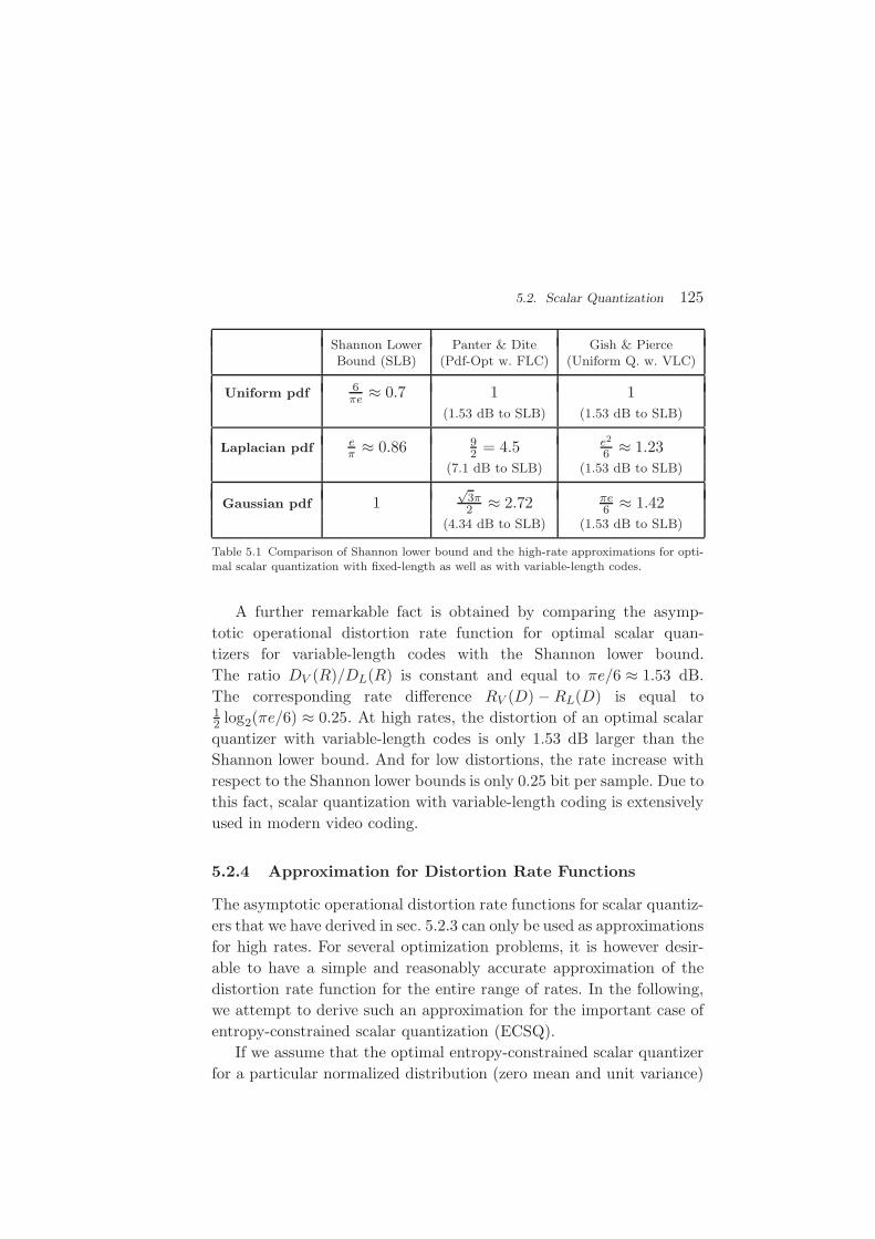
5.2. Scalar Quantization 125
Shannon Lower Panter & Dite Gish & PierceBound (SLB) (Pdf-Opt w. FLC) (Uniform Q. w. VLC)
Uniform pdf6πe ≈ 0.7 1 1
(1.53 dB to SLB) (1.53 dB to SLB)
Laplacian pdfeπ ≈ 0.86 9
2 = 4.5 e2
6 ≈ 1.23
(7.1 dB to SLB) (1.53 dB to SLB)
Gaussian pdf 1√
3π2 ≈ 2.72 πe
6 ≈ 1.42
(4.34 dB to SLB) (1.53 dB to SLB)
Table 5.1 Comparison of Shannon lower bound and the high-rate approximations for opti-mal scalar quantization with fixed-length as well as with variable-length codes.
A further remarkable fact is obtained by comparing the asymp-
totic operational distortion rate function for optimal scalar quan-
tizers for variable-length codes with the Shannon lower bound.
The ratio DV (R)/DL(R) is constant and equal to πe/6 ≈ 1.53 dB.
The corresponding rate difference RV (D)−RL(D) is equal to12 log2(πe/6) ≈ 0.25. At high rates, the distortion of an optimal scalar
quantizer with variable-length codes is only 1.53 dB larger than the
Shannon lower bound. And for low distortions, the rate increase with
respect to the Shannon lower bounds is only 0.25 bit per sample. Due to
this fact, scalar quantization with variable-length coding is extensively
used in modern video coding.
5.2.4 Approximation for Distortion Rate Functions
The asymptotic operational distortion rate functions for scalar quantiz-
ers that we have derived in sec. 5.2.3 can only be used as approximations
for high rates. For several optimization problems, it is however desir-
able to have a simple and reasonably accurate approximation of the
distortion rate function for the entire range of rates. In the following,
we attempt to derive such an approximation for the important case of
entropy-constrained scalar quantization (ECSQ).
If we assume that the optimal entropy-constrained scalar quantizer
for a particular normalized distribution (zero mean and unit variance)

126 Quantization
and its operational distortion rate function g(R) are known, the opti-
mal quantizer for the same distribution but with different mean and
variance can be constructed by an appropriate shifting and scaling of
the quantization intervals and reconstruction levels. The distortion rate
function D(R) of the resulting scalar quantizer can then be written as
D(R) = σ2 · g(R), (5.55)
where σ2 denotes the variance of the input distribution. Hence, it is
sufficient to derive an approximation for the normalized operational
distortion rate function g(R).
For optimal ECSQ, the function g(R) and its derivative g′(R) should
have the following properties:
• If no information is transmitted, the distortion should be
equal to the variance of the input signal,
g(0) = 1. (5.56)
• For high rates, g(R) should be asymptotically tight to the
high-rate approximation,
limR→∞
ε2V · 2−2R
g(R)= 1. (5.57)
• For ensuring the mathematical tractability of optimization
problems the derivative g′(R) should be continuous.
• An increase in rate should result in a distortion reduction,
g′(R) < 0 for R ∈ [0,∞). (5.58)
A function that satisfies the above conditions is
g(R) =ε2V
a· ln(a · 2−2R + 1). (5.59)
The factor a is chosen in a way that g(0) is equal to 1. By numerical
optimization, we obtained a = 0.9519 for the Gaussian pdf and a = 0.5
for the Laplacian pdf. For proving that condition (5.57) is fulfilled, we
can substitute x = 2−2R and develop the Taylor series of the resulting
function
g(x) =ε2
aln(a · x + 1) (5.60)

5.2. Scalar Quantization 127
Fig. 5.12 Operational distortion rate functions for a Gaussian (left) and Laplacian (right)pdf with unit variance. The diagrams show the (information) distortion rate function, thehigh-rate approximation ε2
V 2−2R, and the approximation g(R) given in (5.59). Additionally,results of the EC-Lloyd algorithm with the rate being measured as entropy are shown.
around x0 = 0, which gives
g(x) ≈ g(0) + g′(0) · x = ε2V · x. (5.61)
Since the remaining terms of the Taylor series are negligible for small
values of x (large rates R), (5.59) approaches the high-rate approxima-
tion ε2V 2−2R as the rate R approaches infinity. The first derivative of
(5.59) is given by
g′(R) = −ε2 · 2 ln 2
a + 22R. (5.62)
It is a continuous and always less than zero.
The quality of the approximations for the operational distortion
rate functions of an entropy-constrained quantizer for a Gaussian and
Laplacian pdf is illustrated in Fig. 5.12. For the Gaussian pdf, the ap-
proximation (5.59) provides a sufficiently accurate match to the results
of the entropy-constrained Lloyd algorithm and will be used later. For
the Laplacian pdf, the approximation is less accurate for low bit rates.
5.2.5 Performance Comparison for Gaussian Sources
In the following, we compare the rate distortion performance of the
discussed scalar quantizers designs with the rate distortion bound for
unit-variance stationary Gauss-Markov sources with ρ = 0 and ρ = 0.9.

128 Quantization
The distortion rate functions for both sources, the operational distor-
tion rates function for PCM (uniform, fixed-rate), the Lloyd design,
and the entropy-constraint Lloyd design (EC-Lloyd), as well as the
Panter & Dite and Gish & Pierce asymptotes are depicted in Fig. 5.13.
The rate for quantizers with fixed-length codes is given by the binary
logarithm of the quantizer size K. For quantizers with variable-length
codes, it is measured as the entropy of the reconstruction levels.
R [bit/symbol]
SNR [dB]
Fig. 5.13 Comparison of the rate distortion performance for Gaussian sources.
The scalar quantizer designs behave identical for both sources as
only the marginal pdf f(s) is relevant for the quantizer design algo-
rithms. For high rates, the entropy-constrained Lloyd design and the
Gish & Pierce approximation yield an SNR that is 1.53 dB smaller
than the (information) distortion rate function for the Gauss-Markov
source with ρ = 0. The rate distortion performance of the quantizers
with fixed-length codes is worse, particularly for rates above 1 bit per
sample. It is, however, important to note that it cannot be concluded
that the Lloyd algorithm yields a worse performance than the entropy-
constrained Lloyd algorithm. Both quantizers are (locally) optimal with
respect to their application area. The Lloyd algorithm results an opti-
mized quantizer for fixed-length coding, while the entropy-constrained
Lloyd algorithm yields on optimized quantizer for variable-length cod-
ing (with an average codeword length close to the entropy).

5.2. Scalar Quantization 129
The distortion rate function for the Gauss-Markov source with
ρ = 0.9 is far away from the operational distortion rate functions of the
investigated scalar quantizer designs. The reason is that we assumed
a lossless coding γ that achieves a rate close to the entropy H(S′) of
the output process. A combination of scalar quantization and advanced
lossless coding techniques that exploit dependencies between the out-
put samples is discussed in the next section.
5.2.6 Scalar Quantization for Sources with Memory
In the previous sections, we concentrated on combinations of scalar
quantization with lossless coding techniques that do not exploit de-
pendencies between the output samples. As a consequence, the rate
distortion performance did only depend on the marginal pdf of the in-
put process, and for stationary sources with memory the performance
was identical to the performance for iid sources with the same marginal
distribution. If we, however, apply scalar quantization to sources with
memory, the output samples are not independent. The dependencies
can be exploited by advanced lossless coding techniques such as condi-
tional Huffman codes, block Huffman codes, or arithmetic codes that
use conditional pmfs in the probability modeling stage.
The design goal of Lloyd quantizers was to minimize the distor-
tion for a quantizer of a given size K. Hence, the Lloyd quantizer de-
sign does not change for source with memory. But the design of the
entropy-constrained Lloyd quantizer can be extended by considering
advanced entropy coding techniques. The conditions for the determi-
nation of the reconstruction levels and interval boundaries (given the
decision thresholds and average codeword lengths) do not change, only
the determination of the average codeword lengths in step 4 of the
entropy-constrained Lloyd algorithm needs to be modified. We can de-
sign a lossless code such as a conditional or block Huffman code based
on the joint pmf of the output samples (which is given by the joint
pdf of the input source and the decision thresholds) and determine the
resulting average codeword lengths. But, following the same arguments
as in sec. 5.2.2, we can also approximate the average codeword lengths
based on the corresponding conditional entropy or block entropy.
130 Quantization
For the following consideration, we assume that the input source is
stationary and that its joint pdf for N successive samples is given by
fN (s). If we employ a conditional lossless code (conditional Huffman
code or arithmetic code) that exploits the conditional pmf of a current
output sample S′ given the last N output samples S′, the average
codeword lengths ℓ(s′i) can be set equal to the ratio of the conditional
entropy H(S′|S′) and the symbol probability p(s′i),
ℓ(s′i) =H(S′|S′)
p(s′i)= − 1
p(s′i)
KN−1∑
k=0
pN+1(s′i, s
′
k) log2pN+1(s
′i, s
′
k)
pN (s′
k), (5.63)
where k is an index that indicates any of the KN combinations of the
last N output samples, p is the marginal pmf of the output samples,
and pN and pN+1 are the joint pmfs for N and N +1 successive output
samples, respectively. It should be noted that the argument of the log-
arithm represents the conditional pmf for an output sample S′ given
the N preceding output samples S′.
Each joint pmf for N successive output samples, including the
marginal pmf p with N =1, is determined by the joint pdf fN of the
input source and the decision thresholds,
pN (s′
k) =
∫ uk+1
uk
fN(s) ds, (5.64)
where uk and uk+1 represent the ordered sets of lower and upper inter-
val boundaries for the vector s′
k of output samples. Hence, the average
codeword length ℓ(s′i) can be directly derived based on the joint pdf
for the input process and the decision thresholds. In a similar way, the
average codeword lengths for block codes of N samples can be approx-
imated based on the block entropy for N successive output samples.
We now investigate the asymptotic operational distortion rate func-
tion for high rates. If we again assume that we employ a conditional
lossless code that exploits the conditional pmf using the preceding N
output samples, the rate R can be approximated by the corresponding
conditional entropy H(Sn|Sn−1, · · · , Sn−N ),
R = −K−1∑
i=0
KN−1∑
k=0
pN+1(s′i, s
′
k) log2pN+1(s
′i, s
′
k)
pN (s′
k). (5.65)

5.2. Scalar Quantization 131
For small quantization intervals ∆i (high rates), we can assume that
the joint pdfs fN for the input sources are nearly constant inside each
N -dimensional hypercube given by a combination of quantization in-
tervals, which yields the approximations
pN (s′
k) = fN (s′
k)∆k and pN+1(s′i, s
′
k) = fN+1(s′i, s
′
k)∆k ∆i,
(5.66)
where ∆k represents the Cartesian product of quantization interval
sizes that are associated with the vector of reconstruction levels s′
k.
By inserting these approximations in (5.65), we obtain
R = −K−1∑
i=0
KN−1∑
k=0
fN+1(s′i, s
′
k)∆k ∆i log2
fN+1(s′i, s
′
k)
fN (s′
k)
−K−1∑
i=0
KN−1∑
k=0
fN+1(s′i, s
′
k)∆k ∆i log2 ∆i. (5.67)
Since we consider the asymptotic behavior for infinitesimal quantiza-
tion intervals, the sums can be replaced by integrals, which gives
R = −∫
R
∫
RN
fn+1(s, s) log2fn+1(s, s)
fN (s)ds ds
−K−1∑
i=0
∫
RN
fn+1(s′i, s) ds
∆i log2 ∆i. (5.68)
The first integral (including the minus sign) is the conditional differ-
ential entropy h(Sn|Sn−1, · · · , Sn−N ) for an input sample given the
preceding N input symbols and the second integral is the value f(s′i)of marginal pdf of the input source. Using the high rate approximation
p(s′i) = f(s′i)∆i, we obtain
R = h(Sn|Sn−1, · · · , Sn−N )− 1
2
K−1∑
i=0
p(s′i) log2 ∆2i , (5.69)
which is similar to (5.49). In the same way as for (5.49) in sec. 5.2.3,
we can now apply Jensen’s inequality and then insert the high rate
approximation (5.41) for the MSE distortion measure. As a consequence
132 Quantization
of Jensen’s inequality, we note that also for conditional lossless codes,
the optimal quantizer design for high rates has uniform quantization
steps sizes. The asymptotic operational distortion rate function for an
optimum quantizer with conditional lossless codes is given by
DC(R) =1
12· 2h(Sn|Sn−1,··· ,Sn−N ) · 2−2R. (5.70)
In comparison to the Gish & Pierce asymptote (5.52), the first-order
differential entropy h(S) is replaced by the conditional entropy given
the N preceding input samples.
In a similar way, we can also derive the asymptotic distortion rate
function for block entropy codes (as the block Huffman code) of size N .
We obtain the result that also for block entropy codes, the optimal
quantizer design for high rates has uniform quantization step sizes.
The corresponding asymptotic operational distortion rate function is
DB(R) =1
12· 2
h(Sn,··· ,Sn+N−1)
N · 2−2R, (5.71)
where h(Sn, . . . , Sn+N−1) denotes the joint differential entropy for N
successive input symbols.
The achievable distortion rate function depends on the complexity
of the applied lossless coding technique (which is basically given by the
parameter N). For investigating the asymptotically achievable opera-
tional distortion rate function for arbitrarily complex entropy coding
techniques, we take the limit for N →∞, which yields
D∞(R) =1
12· 2h(S) · 2−2R, (5.72)
where h(S) denotes the differential entropy rate of the input source.
A comparison with the Shannon lower bound (4.65) shows that the
asymptotically achievable distortion for high rates and arbitrarily com-
plex entropy coding is 1.53 dB larger than the fundamental perfor-
mance bound. The corresponding rate increase is 0.25 bit per sample.
It should be noted that this asymptotic bound can only be achieved for
high rates. Furthermore, in general, the entropy coding would require
the storage of a very large set of codewords or conditional probabilities,
which is virtually impossible in real applications.

5.3. Vector Quantization 133
5.3 Vector Quantization
The investigation of scalar quantization (SQ) showed that it is impos-
sible to achieve the fundamental performance bound using a source
coding system consisting of scalar quantization and lossless coding.
For high rates the difference to the fundamental performance bound is
1.53 dB or 0.25 bit per sample. This gap can only be reduced if mul-
tiple samples are jointly quantized, i.e., by vector quantization (VQ).
Although vector quantization is rarely used in video coding, we will give
a brief overview in order to illustrate its design, performance, complex-
ity, and the reason for the limitation of scalar quantization.
In N -dimensional vector quantization, an input vector s consisting
of N samples is mapped to a set of K reconstruction vectors {s′
i}. We
will generally assume that the input vectors are blocks of N successive
samples of a realization of a stationary random process {S}. Similarly
as for scalar quantization, we restrict our considerations to regular vec-
tor quantizers5 for which the quantization cells are convex sets6 and
each reconstruction vector is an element of the associated quantization
cell. The average distortion and average rate of a vector quantizer are
given by (5.5) and (5.7), respectively.
5.3.1 Vector Quantization with Fixed-Length Codes
We first investigate a vector quantizer design that minimizes the dis-
tortion D for a given quantizer size K, i.e., the counterpart of the Lloyd
quantizer. The necessary conditions for the reconstruction vectors and
quantization cells can be derived in the same way as for the Lloyd
quantizer in sec. 5.2.1 and are given by
s′
i = arg mins′∈RN
E{dN(S, s′) | S ∈ Ci} , (5.73)
and
Q(s) = arg min∀s′
i
dN (s, s′
i). (5.74)
5 Regular quantizers are optimal with respect to the MSE distortion measure.6 A set of points in RN is convex, if for any two points of the set, all points on the straightline connecting the two points are also elements of the set.

134 Quantization
The Linde-Buzo-Gray Algorithm. The extension of the Lloyd al-
gorithm to vector quantization [46] is referred to as Linde-Buzo-Gray
algorithm (LBG). For a sufficiently large training set {sn} and a given
quantizer size K, the algorithm can be stated as follows:
(1) Choose an initial set of reconstruction vectors {s′
i}.(2) Associate all samples of the training set {sn} with one of the
quantization cells Ci according to
a(sn) = arg min∀i
dN (sn, s′
i).
(3) Update the reconstruction vectors {s′
i} according to
s′
i = arg mins′∈RN
E{dN(S, s′) | α(S) = i} ,
where the expectation value is taken over the training set.
(4) Repeat the previous two steps until convergence.
Examples for the LBG Algorithm. An an example, we designed
a 2-d vector quantizer for a Gaussian iid process with unit variance.
The selected quantizer size is K = 16 corresponding to a rate of 2 bit
per (scalar) sample. The chosen initialization as well as the obtained
quantization cells and reconstruction vectors after the 8-th and 49-th
iteration of the LBG algorithm are illustrated in Fig. 5.14. In Fig. 5.15,
the distortion is plotted as function of the iteration step.
initialization after iteration 8 after iteration 49
Fig. 5.14 Illustration of the LBG algorithm for a quantizer with N = 2 and K = 16 and aGaussian iid process with unit variance. The lines mark the boundaries of the quantizationcells, the crosses show the reconstruction vectors, and the light-colored dots represent thesamples of the training set.

5.3. Vector Quantization 135
Fig. 5.15 Distortion as function of the iteration step for the LBG algorithm with N = 2,K = 16, and a Gaussian iid process with unit variance. The dashed line represents thedistortion for a Lloyd quantizer with the same rate of R = 2 bit per sample.
After the 8-th iteration, the 2-dimensional vector quantizer shows a
similar distortion (9.30 dB) as the scalar Lloyd quantizer at the same
rate of R = 2 bit per (scalar) sample. This can be explained by the
fact that the quantization cells are approximately rectangular shaped
and that such rectangular cells would also be constructed by a corre-
sponding scalar quantizer (if we illustrate the result for 2 consecutive
samples). After the 49-th iteration, the cells of the vector quantizer are
shaped in a way that a scalar quantizer cannot create and the SNR is
improved to 9.67 dB.
0 10 20 30 40 5002468
1012141618202224
Iteration
SN
R [d
B],
H [b
it/s]
1.31 dB
H=3.69 bit/s
Conjectured VQ performance for R=4 bit/s
Fixed−length SQ performance for R=4 bit/s
Fig. 5.16 Illustration of the LBG algorithm for a quantizer with N = 2 and K = 256 and aGaussian iid process with unit variance: (left) resulting quantization cells and reconstructionvectors after 49 iterations; (right) distortion as function of the iteration step.

136 Quantization
0 10 20 30 40 5002468
1012141618202224
Iteration
SN
R [d
B],
H [b
it/s] 2.44 dB
H=3.44 bit/s
Conjectured VQ performance for R=4 bit/s
Fixed−length SQ performance for R=4 bit/s
Fig. 5.17 Results of the LBG algorithm for a 2-d VQ with a size of K = 16 (top) andK = 256 (bottom) for a Laplacian iid source with unit variance.
Fig. 5.16 shows the result of the LBG algorithm for a vector quan-
tizer with N = 2 and K = 256, corresponding to a rate of R = 4 bit
per sample, for the Gaussian iid source with unit variance. After the
49-th iteration, the gain for two-dimensional VQ is around 0.9 dB com-
pared to SQ with fixed-length codes resulting in an SNR of 20.64 dB
(of conjectured 21.05 dB [50]). The result indicates that at higher bit
rates, the gain of VQ relative to SQ with fixed-length codes increases.
Fig. 5.17 illustrates the results for a 2-d VQ design for a Laplacian
iid source with unit variance and two different quantizer sizes K. For
K = 16, which corresponds to a rate of R = 2 bit per sample, the SNR
is 8.87 dB. Compared to SQ with fixed-length codes at the same rate,
a gain of 1.32 dB has been achieved. For a rate of R = 4 bit per sample
(K = 256), the SNR gain is increased to 1.84 dB resulting in an SNR
of 19.4 dB (of conjectured 19.99 dB [50]).
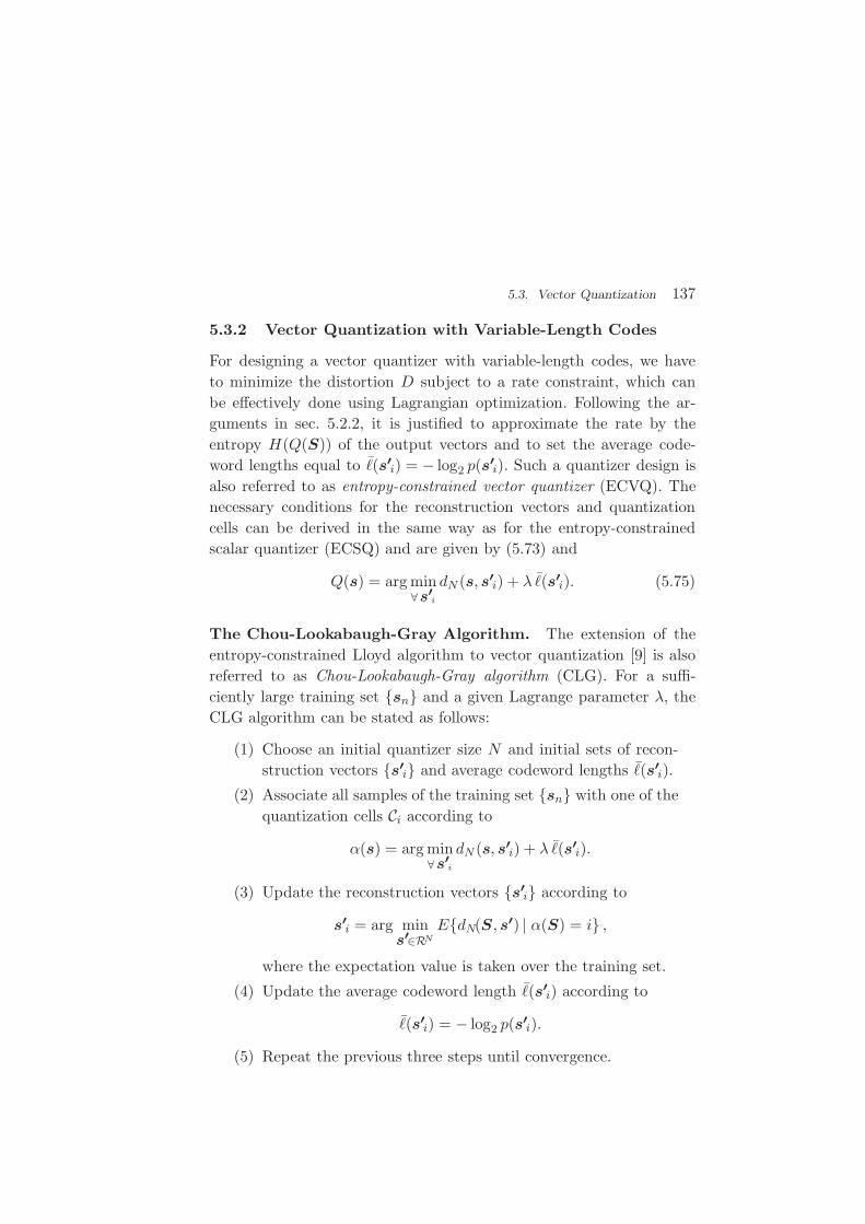
5.3. Vector Quantization 137
5.3.2 Vector Quantization with Variable-Length Codes
For designing a vector quantizer with variable-length codes, we have
to minimize the distortion D subject to a rate constraint, which can
be effectively done using Lagrangian optimization. Following the ar-
guments in sec. 5.2.2, it is justified to approximate the rate by the
entropy H(Q(S)) of the output vectors and to set the average code-
word lengths equal to ℓ(s′
i) = − log2 p(s′
i). Such a quantizer design is
also referred to as entropy-constrained vector quantizer (ECVQ). The
necessary conditions for the reconstruction vectors and quantization
cells can be derived in the same way as for the entropy-constrained
scalar quantizer (ECSQ) and are given by (5.73) and
Q(s) = arg min∀s′
i
dN (s, s′
i) + λ ℓ(s′
i). (5.75)
The Chou-Lookabaugh-Gray Algorithm. The extension of the
entropy-constrained Lloyd algorithm to vector quantization [9] is also
referred to as Chou-Lookabaugh-Gray algorithm (CLG). For a suffi-
ciently large training set {sn} and a given Lagrange parameter λ, the
CLG algorithm can be stated as follows:
(1) Choose an initial quantizer size N and initial sets of recon-
struction vectors {s′
i} and average codeword lengths ℓ(s′
i).
(2) Associate all samples of the training set {sn} with one of the
quantization cells Ci according to
α(s) = arg min∀s′
i
dN (s, s′
i) + λ ℓ(s′
i).
(3) Update the reconstruction vectors {s′
i} according to
s′
i = arg mins′∈RN
E{dN(S, s′) | α(S) = i} ,
where the expectation value is taken over the training set.
(4) Update the average codeword length ℓ(s′
i) according to
ℓ(s′
i) = − log2 p(s′
i).
(5) Repeat the previous three steps until convergence.

138 Quantization
Examples for the CLG Algorithm. As examples, we designed a
2-d ECVQ for a Gaussian and Laplacian iid process with unit variance
and an average rate, measured as entropy, of R = 2 bit per sample.
The results of the CLG algorithm are illustrated in Fig. 5.18. The SNR
gain compared to an ECSQ design with the same rate is 0.26 dB for
the Gaussian and 0.37 dB for the Laplacian distribution.
Fig. 5.18 Results of the CLG algorithm for a Gaussian (top) and Laplacian (bottom) iidsource with unit variance and a rate (entropy) of R = 2 bit per sample. The dashed line inthe diagrams on the right shows the distortion for an ECSQ design with the same rate.
5.3.3 The Vector Quantization Advantage
The examples for the LBG and CLG algorithms showed that vector
quantization increases the coding efficiency compared to scalar quan-
tization. According to the intuitive analysis in [52], the performance
gain can be attributed to three different effects: the space filling advan-
tage, the shape advantage, and the memory advantage. In the following,

5.3. Vector Quantization 139
we will briefly explain and discuss these advantages. We will see that
the space filling advantage is the only effect that can be exclusively
achieved with vector quantization. The associated performance gain
is bounded to 1.53 dB or 0.25 bit per sample. This bound is asymp-
totically achieved for large quantizer dimensions and large rates, and
corresponds exactly to the gap between the operational rate distor-
tion function for scalar quantization with arbitrarily complex entropy
coding and the rate distortion bound at high rates. For a deeper anal-
ysis of the vector quantization advantages, the reader is referred to the
discussion in [52] and the quantitative analysis in [50].
Space Filling Advantage. When we analyze the results of scalar
quantization in higher dimension, we see that the N -dimensional space
is partitioned into N -dimensional hyperrectangles (Cartesian products
of intervals). This does however not represent the densest packing
in RN . With vector quantization of dimension N , we have extra free-
dom in choosing the shapes of the quantization cells. The associated
increase in coding efficiency is referred to as space filling advantage.
The space filling advantage can be observed in the example for the
LBG algorithm with N = 2 and a Gaussian iid process in Fig. 5.14.
After the 8-th iteration, the distortion is approximately equal to the
distortion of the scalar Lloyd quantizer with the same rate and the re-
construction cells are approximately rectangular shaped. However, the
densest packing in two dimensions is achieved by hexagonal quantiza-
tion cells. After the 49-th iteration of the LBG algorithm, the quan-
tization cells in the center of the distribution look approximately like
hexagons. For higher rates, the convergence toward hexagonal cells is
even better visible as can be seen in Figs. 5.16 and 5.17
To further illustrate the space filling advantage, he have conducted
another experiment for a uniform iid process with A = 10. The op-
erational distortion rate function for scalar quantization is given by
D(R) = A2
12 2−2R. For a scalar quantizer of size K = 10, we obtain a
rate (entropy) of 3.32 bit per sample and a distortion of 19.98 dB.
The LBG design with N = 2 and K = 100 is associated with about the
same rate. The partitioning converges toward a hexagonal lattice as
illustrated in Fig. 5.19 and the SNR is increased to 20.08 dB.
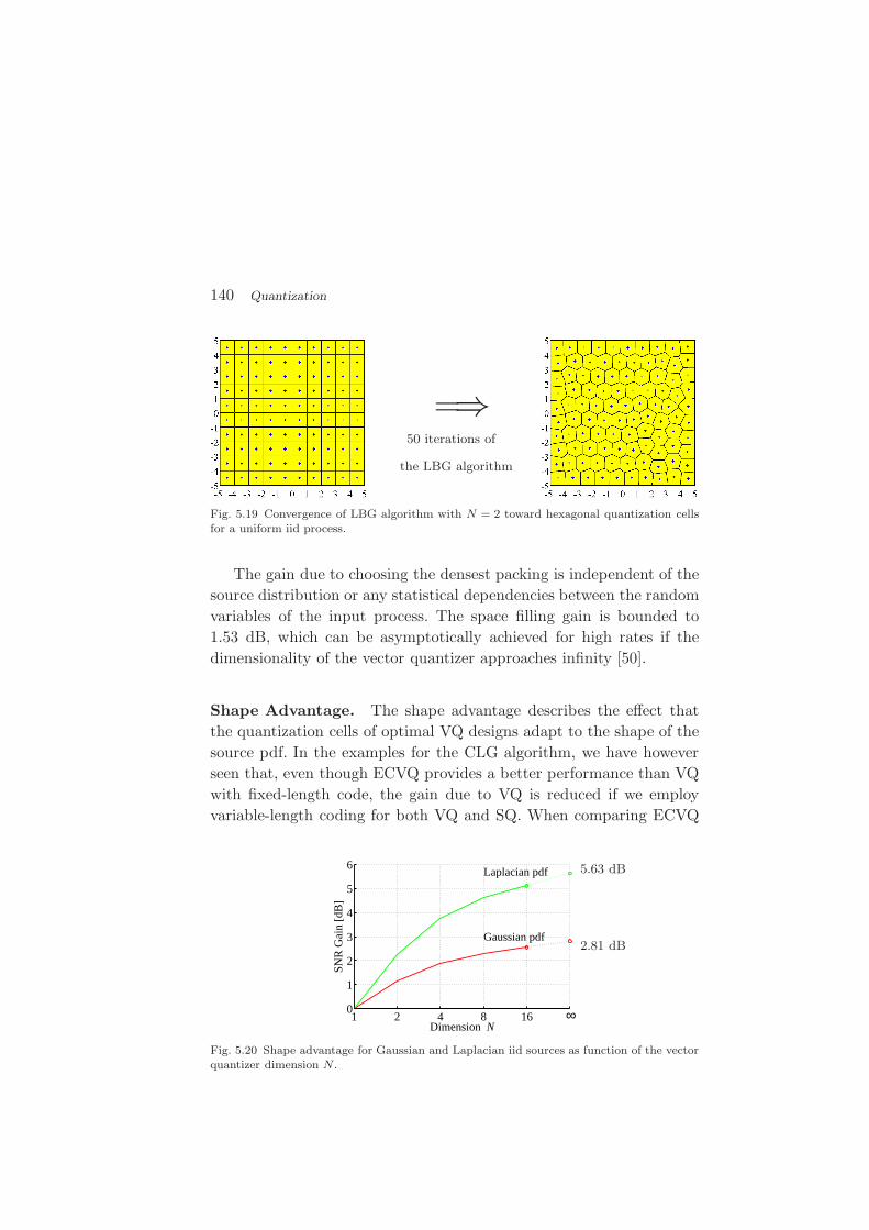
140 Quantization
=⇒50 iterations of
the LBG algorithm
Fig. 5.19 Convergence of LBG algorithm with N = 2 toward hexagonal quantization cellsfor a uniform iid process.
The gain due to choosing the densest packing is independent of the
source distribution or any statistical dependencies between the random
variables of the input process. The space filling gain is bounded to
1.53 dB, which can be asymptotically achieved for high rates if the
dimensionality of the vector quantizer approaches infinity [50].
Shape Advantage. The shape advantage describes the effect that
the quantization cells of optimal VQ designs adapt to the shape of the
source pdf. In the examples for the CLG algorithm, we have however
seen that, even though ECVQ provides a better performance than VQ
with fixed-length code, the gain due to VQ is reduced if we employ
variable-length coding for both VQ and SQ. When comparing ECVQ
1 2 4 8 160
1
2
3
4
5
6
Dimension N
SN
R G
ain
[dB
]
Gaussian pdf
Laplacian pdf
∞
5.63 dB
2.81 dB
Fig. 5.20 Shape advantage for Gaussian and Laplacian iid sources as function of the vectorquantizer dimension N .

5.3. Vector Quantization 141
with ECSQ for iid sources, the gain of VQ reduces to the space filling
advantage, while the shape advantage is exploited by variable-length
coding. However, VQ with fixed-length codes can also exploit the gain
that ECSQ shows compared to SQ with fixed-length codes [50].
The shape advantage for high rates has been estimated in [50].
Fig. 5.20 shows this gain for Gaussian and Laplacian iid random pro-
cesses. In practice, the shape advantage is exploited by using scalar
quantization in combination with entropy coding techniques such as
Huffman coding or arithmetic coding.
Memory Advantage. For sources with memory, there are linear or
nonlinear dependencies between the samples. In optimal VQ designs,
the partitioning of the N -dimensional space into quantization cells is
chosen in a way that these dependencies are exploited. This is illus-
trated in Fig. 5.21, which shows the ECVQ result of the CLG algo-
rithm for N = 2 and a Gauss-Markov process with a correlation factor
of ρ = 0.9 for two different values of the Lagrange parameter λ.
Fig. 5.21 Results of the CLG algorithm with N = 2 and two different values of λ for aGauss-Markov source with ρ = 0.9.
An quantitative estimation of the gain resulting from the memory
advantage at high rates was done in [50]. Fig. 5.22 shows the mem-
ory gain for Gauss-Markov sources with different correlation factors as
function of the quantizer dimension N .
For sources with strong dependencies between the samples, such as
video signals, the memory gain is much larger than the shape and space
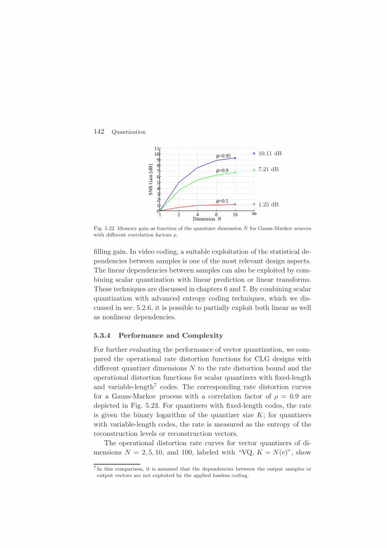
142 Quantization
1 2 4 8 160123456789
1011
Dimension N
SN
R G
ain
[dB
]
ρ=0.5
ρ=0.9
ρ=0.95
∞
10.11 dB
7.21 dB
1.25 dB
Fig. 5.22 Memory gain as function of the quantizer dimension N for Gauss-Markov sourceswith different correlation factors ρ.
filling gain. In video coding, a suitable exploitation of the statistical de-
pendencies between samples is one of the most relevant design aspects.
The linear dependencies between samples can also be exploited by com-
bining scalar quantization with linear prediction or linear transforms.
These techniques are discussed in chapters 6 and 7. By combining scalar
quantization with advanced entropy coding techniques, which we dis-
cussed in sec. 5.2.6, it is possible to partially exploit both linear as well
as nonlinear dependencies.
5.3.4 Performance and Complexity
For further evaluating the performance of vector quantization, we com-
pared the operational rate distortion functions for CLG designs with
different quantizer dimensions N to the rate distortion bound and the
operational distortion functions for scalar quantizers with fixed-length
and variable-length7 codes. The corresponding rate distortion curves
for a Gauss-Markov process with a correlation factor of ρ = 0.9 are
depicted in Fig. 5.23. For quantizers with fixed-length codes, the rate
is given the binary logarithm of the quantizer size K; for quantizers
with variable-length codes, the rate is measured as the entropy of the
reconstruction levels or reconstruction vectors.
The operational distortion rate curves for vector quantizers of di-
mensions N = 2, 5, 10, and 100, labeled with “VQ, K = N(e)”, show
7 In this comparison, it is assumed that the dependencies between the output samples oroutput vectors are not exploited by the applied lossless coding.

5.3. Vector Quantization 143
Fixed-Length Coded SQ (K=1) !
(Panter-Dite Approximation)!
ECSQ using EC Lloyd Algorithm!
VQ, K=2 (e)!
VQ, K=2 using LBG algorithm!
VQ, K=5 (e)!
VQ, K=10 (e)!
VQ, K=100 (e)!
R(D)!
SNR [dB]!
R [bit/scalar]!
Fig. 5.23 Estimated vector quantization advantage at high rates [50] for a Gauss-Markovsource with a correlation factor of ρ = 0.9.
the theoretical performance for high rates, which has been estimated
in [50]. These theoretical results have been verified for N = 2 by design-
ing entropy-constrained vector quantizers using the CLG algorithm.
The theoretical vector quantizer performance for a quantizer dimension
of N = 100 is very close to the distortion rate function of the inves-
tigated source. In fact, vector quantization can asymptotically achieve
the rate distortion bound as the dimension N approaches infinity. More-
over, vector quantization can be interpreted as the most general lossy
source coding system. Each source coding system that maps a vector
of N samples to one of K codewords (or codeword sequences) can be
designed as vector quantizer of dimension N and size K.
Despite the excellent coding efficiency vector quantization is rarely
used in video coding. The main reason is the associated complexity.
On one hand, a general vector quantizer requires the storage of a large
codebook. This issue becomes even more problematic for systems that
must be able to encode and decode sources at different bit rates, as it
is required for video codecs. On the other hand, the computationally

144 Quantization
complexity for associating an input vector with the best reconstruction
vector in rate distortion sense is very large in comparison to the encod-
ing process for scalar quantization that is used in practice. One way to
reduce the requirements on storage and computational complexity is
to impose structural constraints on the vector quantizer. Examples for
such structural constraints include:
• Tree-Structured VQ,• Transform VQ,• Multistage VQ,• Shape-Gain VQ,• Lattice Codebook VQ,• Predictive VQ.
In particular, predictive VQ can be seen as a generalization of a number
of very popular techniques including motion compensation in video cod-
ing. For the actual quantization, video codecs mostly include a simple
scalar quantizer with uniformly distributed reconstruction levels (some-
times with a deadzone around zero), which is combined with entropy
coding and techniques such as linear prediction or linear transforms in
order to exploit the shape of the source distribution and the statistical
dependencies of the source. For video coding, the complexity of vector
quantizers including those with structural constraints is considered as
too large in relation to the achievable performance gains.
5.4 Summary of Quantization
In this chapter, we have discussed quantization starting with scalar
quantizers. The Lloyd quantizer that is constructed using an iterative
procedure provides the minimum distortion for a given number of re-
construction levels. It is the optimal quantizer design if the reconstruc-
tion levels are transmitted using fixed-length codes. The extension of
the quantizer design for variable-length codes is achieved by minimiz-
ing the distortion D subject to a rate constraint R < Rmax, which can
be formulated as a minimization of a Lagrangian functional D + λR.
The corresponding iterative design algorithm includes a sufficiently ac-
curate estimation of the codeword lengths that are associated with the

5.4. Summary of Quantization 145
reconstruction levels. Usually the codeword lengths are estimated based
on the entropy of the output signal, in which case the quantizer design
is also referred to as entropy-constrained Lloyd quantizer.
At high rates, the operational distortion rate functions for scalar
quantization with fixed- and variable-length codes as well as the Shan-
non lower bound can be described by
DX(R) = σ2 · ε2X · 2−2R, (5.76)
where X either indicates the Shannon lower bound or scalar quantiza-
tion with fixed- or variable-length codes. For a given X, the factors ε2X
depend only of the statistical properties of the input source. If the
output samples are coded with an arbitrarily complex entropy coding
scheme, the difference between the operational distortion rate function
for optimal scalar quantization and the Shannon lower bound is 1.53 dB
or 0.25 bit per sample at high rates. Another remarkable result is that
at high rates, optimal scalar quantization with variable-length codes is
achieved if all quantization intervals have the same size.
In the second part of the chapter, we discussed the extension of
scalar quantization to vector quantization, by which the rate distortion
bound can be asymptotically achieved as the quantizer dimension ap-
proaches infinity. The coding efficiency improvements of vector quanti-
zation relative to scalar quantization can be attributed to three different
effects: the space filling advantage, the shape advantage, and the mem-
ory advantage. While the space filling advantage can be only achieved
by vector quantizers, the shape and memory advantage can also be ex-
ploited by combining scalar quantization with a suitable entropy coding
and techniques such as linear prediction and linear transforms.
Despite its superior rate distortion performance, vector quantization
is rarely used in video coding applications because of its complexity.
Instead, modern video codecs combine scalar quantization with entropy
coding, linear prediction, and linear transforms in order to achieve a
high coding efficiency at a moderate complexity level.

6
Predictive Coding
In the previous chapter, we investigated the design and rate distortion
performance of quantizers. We showed that the fundamental rate dis-
tortion bound can be virtually achieved by unconstrained vector quan-
tization of a sufficiently large dimension. However, due to the very large
amount of data in video sequences and the real-time requirements that
are found in most video coding applications, only low-complex scalar
quantizers are typically used in this area. For iid sources, the achievable
operational rate distortion function for high rate scalar quantization
lies at most 1.53 dB or 0.25 bit per sample above the fundamental rate
distortion bound. This represents a suitable trade-off between coding
efficiency and complexity. But if there is a large amount of dependen-
cies between the samples of an input signal, as it is the case in video
sequences, the rate distortion performance for simple scalar quantizers
becomes significantly worse than the rate distortion bound. A source
coding system consisting of a scalar quantizer and an entropy coder
can exploit the statistical dependencies in the input signal only if the
entropy coder uses higher-order conditional or joint probability mod-
els. The complexity of such an entropy coder is however close to that
of a vector quantizer, so that such a design is unsuitable in practice.
146

147
Furthermore, video sequences are highly nonstationary and conditional
or joint probabilities for nonstationary sources are typically very dif-
ficult to estimate accurately. It is desirable to combine scalar quanti-
zation with additional tools that can efficiently exploit the statistical
dependencies in a source at a low complexity level. One of such coding
concepts is predictive coding, which we will investigate in this chap-
ter. The concepts of prediction and predictive coding are widely used
in modern video coding. Well-known examples are intra prediction,
motion-compensated prediction, and motion vector prediction.
Q! +!+!
ˆ S n
ˆ S n
Sn
" S n
Un
" U n
-!
Fig. 6.1 Basic structure of predictive coding.
The basic structure of predictive coding is illustrated in Fig. 6.1
using the notation of random variables. The source samples {sn} are
not directly quantized. Instead, each sample sn is predicted based on
previous samples. The prediction value sn is subtracted from the value
of the input sample sn yielding a residual or prediction error sample
un = sn − sn. The residual sample un is then quantized using scalar
quantization. The output of the quantizer is a reconstructed value u′n
for the residual sample un. At the decoder side, the reconstruction u′n
of the residual sample is added to the predictor sn yielding the recon-
structed output sample s′n = sn + u′n.
Intuitively, we can say that the better the future of a random pro-
cess is predicted from its past and the more redundancy the random
process contains, the less new information is contributed by each suc-
cessive observation of the process. In the context of predictive coding,
the predictors sn should be chosen in a way that they can be easily
computed and result in a rate distortion efficiency of the predictive
coding system that is as close as possible to the rate distortion bound.
In this chapter, we discuss the design of predictors with the em-
phasis on linear predictors and analyze predictive coding systems. For
further details, the reader is referred to the classic tutorial [51], and
the detailed treatments in [75] and [24].

148 Predictive Coding
6.1 Prediction
Prediction is a statistical estimation procedure where the value of a par-
ticular random variable Sn of a random process {Sn} is estimated based
on the values of other random variables of the process. Let Bn be a set of
observed random variables. As a typical example, the observation set
can represent the N random variables Bn = {Sn−1, Sn−2, · · · , Sn−N}that precede that random variable Sn to be predicted. The predictor
for the random variable Sn is a deterministic function of the observa-
tion set Bn and is denoted by An(Bn). In the following, we will omit this
functional notation and consider the prediction of a random variable Sn
as another random variable denoted by Sn,
Sn = An(Bn). (6.1)
The prediction error or residual is given by the difference of the ran-
dom variable Sn to be predicted and its prediction Sn. It can also be
interpreted as a random variable and is be denoted Un,
Un = Sn − Sn. (6.2)
If we predict all random variables of a random process {Sn}, the se-
quence of predictions {Sn} and the sequence of residuals {Un} are ran-
dom processes. The prediction can then be interpreted as a mapping
of an input random process {Sn} to an output random process {Un}representing the sequence of residuals as illustrated in Fig. 6.2.
Predictor!
+!
ˆ S n
Sn
Un-!
Fig. 6.2 Block diagram of a predictor.
In order to derive optimum predictors, we have to discuss first how
the goodness of a predictor can be evaluated. In the context of pre-
dictive coding, the ultimate goal is to achieve the minimum distortion
between the original and reconstructed samples subject to a given max-
imum rate. For the MSE distortion measure (or in general for all ad-
ditive difference distortion measures), the distortion between a vector

6.1. Prediction 149
of N input samples s and the associated vector of reconstructed sam-
ples s′ is equal to the distortion between the corresponding vector of
residuals u and the associated vector of reconstructed residuals u′,
dN (s, s′) =1
N
N−1∑
i=0
(si − s′i)2 =
1
N
N−1∑
i=0
(ui + si − u′i − si)
2 = dN (u,u′).
(6.3)
Hence, the operational distortion rate function of a predictive coding
systems is equal to the operational distortion rate function for scalar
quantization of the prediction residuals. As stated in sec. 5.2.4, the
operational distortion rate curve for scalar quantization of the resid-
uals can be stated as D(R) = σ2U · g(R), where σ2
U is the variance of
the residuals and the function g(R) depends only on the type of the
distribution of the residuals. Hence, the rate distortion efficiency of a
predictive coding system depends on the variance of the residuals and
the type of their distribution. We will neglect the dependency on the
distribution type and define that a predictor An(Bn) given an observa-
tion set Bn is optimal if it minimizes the variance σ2U of the prediction
error. In the literature [51, 75, 24], the most commonly used criterion
for the optimality of a predictor is the minimization of the MSE be-
tween the input signal and its prediction. This is equivalent to the
minimization of the second moment ǫ2U = σ2
U + µ2U , or the energy, of
the prediction error signal. Since the minimization of the second mo-
ment ǫ2U implies1 a minimization of the variance σ2
U and the mean µU ,
we will also consider the minimization of the mean squared prediction
error ǫ2U .
When considering the more general criterion of the mean squared
prediction error, the selection of the optimal predictor An(Bn) given
an observation set Bn is equivalent to the minimization of
ǫ2U = E
{U2
n
}= E
{(Sn − Sn
)2}
= E{(
Sn −An(Bn))2}
. (6.4)
The solution to this minimization problem is given by the conditional
mean of the random variable Sn given the observation set Bn,
S∗n = A∗
n(Bn) = E{Sn | Bn} . (6.5)
1 We will later prove this statement for linear prediction.

150 Predictive Coding
This can be proved by using the formulation
ǫ2U = E
{(Sn − E{Sn | Bn}+ E{Sn | Bn} −An(Bn)
)2}
= E{(
Sn − E{Sn | Bn})2}
+(E{Sn | Bn} −An(Bn)
)2 −2E{(
Sn − E{Sn | Bn})(
E{Sn | Bn} −An(Bn))}
. (6.6)
Since E{Sn | Bn} and An(Bn) are deterministic functions given the ob-
servation set Bn, we can write
E{(
Sn − E{Sn | Bn})(
E{Sn | Bn} −An(Bn))| Bn
}
=(E{Sn | Bn} −An(Bn)
)· E{Sn − E{Sn | Bn} | Bn}
=(E{Sn | Bn} −An(Bn)
)·(E{Sn | Bn} − E{Sn | Bn}
)
= 0. (6.7)
By using the iterative expectation rule E{E{g(S)|X}} = E{g(S)},which was derived in (2.32), we obtain for the cross term in (6.6),
E{(
Sn − E{Sn | Bn})(
E{Sn | Bn} −An(Bn))}
= E{E{(
Sn − E{Sn | Bn})(
E{Sn | Bn} −An(Bn))| Bn
}}
= E{0} = 0. (6.8)
Inserting this relationship into (6.6) yields
ǫ2U = E
{(Sn − E{Sn | Bn}
)2}
+(E{Sn | Bn} −An(Bn)
)2, (6.9)
which proves that the conditional mean E{Sn | Bn}minimizes the mean
squared prediction error for a given observation set Bn.
We will show later that in predictive coding the observation set Bn
must consist of reconstructed samples. If we for example use the last
N reconstructed samples as observation set, Bn = {S′n−1, · · · , S′
n−N},it is conceptually possible to construct a table in which the conditional
expectations E{Sn | s′n−1, · · · , s′n−N
}are stored for all possible com-
binations of the values of s′n−1 to s′n−N . This is in some way similar
to scalar quantization with an entropy coder that employs the con-
ditional probabilities p(sn | s′n−1, · · · , s′n−N ) and does not significantly
reduce the complexity. For obtaining a low-complexity alternative to
this scenario, we have to introduce structural constraints for the pre-
dictor An(Bn). Before we state a reasonable structural constraint, we
derive the optimal predictors according to (6.5) for two examples.

6.1. Prediction 151
Stationary Gaussian Sources. As a first example, we consider a
stationary Gaussian source and derive the optimal predictor for a
random variable Sn given a vector Sn−k = (Sn−k, · · · , Sn−k−N+1)T ,
with k > 0, of N preceding samples. The conditional distribution
f(Sn |Sn−k) of jointly Gaussian random variables is also Gaussian.
The conditional mean E{Sn |Sn−k} and thus the optimal predictor is
given by (see for example [26])
An(Sn−k) = E{Sn |Sn−k} = µS + cTk C−1
N (Sn−k − µS eN ), (6.10)
where µS represents the mean of the Gaussian process, eN is the
N -dimensional vector with all elements equal to 1, and CN is the N -th
order autocovariance matrix, which is given by
CN = E{(Sn − µS eN )(Sn − µS eN )T
}. (6.11)
The vector ck is an autocovariance vector and is given by
ck = E{(Sn − µ)(Sn−k − µS eN )} . (6.12)
Autoregressive Processes. Autoregressive processes are an impor-
tant model for random sources. An autoregressive process of order m,
also referred to as AR(m) process, is given by the recursive formula
Sn = Zn + µS +m∑
i=1
ai (Sn−1 − µS)
= Zn + µS(1− aTmem) + aT
mS(m)n−1, (6.13)
where µS is the mean of the random process, am = (a1, · · · , am)T is
a constant parameter vector, and {Zn} is a zero-mean iid process.
We consider the prediction of a random variable Sn given the vec-
tor Sn−1 of the N directly preceding samples, where N is greater than
or equal to the order m. The optimal predictor is given by the con-
ditional mean E{Sn |Sn−1}. By defining an N -dimensional parameter
vector aN = (a1, · · · , am, 0, · · · , 0)T , we obtain
E{Sn |Sn−1} = E{Zn + µS(1− aT
NeN ) + aTN Sn−1 |Sn−1
}
= µS(1− aTNeN ) + aT
N Sn−1. (6.14)
152 Predictive Coding
For both considered examples, the optimal predictor is given by
a linear function of the observation vector. In a strict sense, it is an
affine function if the mean µ of the considered processes is nonzero. If
we only want to minimize the variance of the prediction residual, we
do not need the constant offset and can use strictly linear predictors.
For predictive coding systems, affine predictors have the advantage
that the scalar quantizer can be designed for zero-mean sources. Due
to their simplicity and their effectiveness for a wide range of random
processes, linear (and affine) predictors are the most important class
of predictors for video coding applications. It should however be noted
that nonlinear dependencies in the input process cannot be exploited
using linear or affine predictors. In the following, we will concentrate
on the investigation of linear prediction and linear predictive coding.
6.2 Linear Prediction
In the following, we consider linear and affine prediction of a random
variable Sn given an observation vector Sn−k = [Sn−k, · · · , Sn−k−N+1]T,
with k > 0, of N preceding samples. We restrict our considerations to
stationary processes. In this case, the prediction function An(Sn−k)
is independent of the time instant of the random variable to be pre-
dicted and is denoted by A(Sn−k). For the more general affine form,
the predictor is given by
Sn = A(Sn−k) = h0 + hTNSn−k, (6.15)
where the constant vector hN = (h1, · · · , hN )T and the constant off-
set h0 are the parameters that characterize the predictor. For linear
predictors, the constant offset h0 is equal to zero.
The variance σ2U of the prediction residual depends on the predictor
parameters and can be written as
σ2U (h0,hN ) = E
{(Un−E{Un}
)2}
= E{(
Sn−h0−hTNSn−k − E
{Sn−h0−hT
NSn−k
} )2}
= E{(
Sn−E{Sn} − hTN
(Sn−k−E{Sn−k}
))2}
. (6.16)
The constant offset h0 has no influence on the variance of the residual.
6.2. Linear Prediction 153
The variance σ2U depends only on the parameter vector hN . By further
reformulating the expression (6.16), we obtain
σ2U (hN ) = E
{(Sn−E{Sn}
)2}
− 2 hTN E
{(Sn−E{Sn}
)(Sn−k−E{Sn−k}
)}
+ hTN E
{(Sn−k−E{Sn−k}
)(Sn−k−E{Sn−k}
)T}
hN
= σ2S − 2hT
N ck + hTN CN hN , (6.17)
where σ2S is the variance of the input process and CN and ck are the au-
tocovariance matrix and the autocovariance vector of the input process
given by (6.11) and (6.12), respectively.
The mean squared prediction error is given by
ǫ2U (h0,hN ) = σ2
U (hN ) + µ2U (h0,hN )
= σ2U (hN ) + E
{Sn − h0 − hT
N Sn−k
}2
= σ2U (hN ) +
(µS(1− hT
NeN )− h0
)2, (6.18)
with µS being the mean of the input process and eN denoting the
N -dimensional vector with all elements are equal to 1. Consequently,
the minimization of the mean squared prediction error ǫ2U is equivalent
to choosing the parameter vector hN that minimizes the variance σ2U
and additionally setting the constant offset h0 equal to
h∗0 = µS (1− hT
N eN ). (6.19)
This selection of h0 yields a mean of µU =0 for the prediction error
signal, and the MSE between the input signal and the prediction ǫ2U is
equal to the variance of the prediction residual σ2U . Due to this simple
relationship, we restrict the following considerations to linear predictors
Sn = A(Sn−k) = hTN Sn−k (6.20)
and the minimization of the variance σ2U . But we keep in mind that the
affine predictor that minimizes the mean squared prediction error can
be obtained by additionally selecting an offset h0 according to (6.19).
The structure of a linear predictor is illustrated in Fig. 6.3.

154 Predictive Coding
Sn
ˆ S n
z"1
h1
z"1
+!
h2
z"1
+!
hN
+-!
Un
Fig. 6.3 Structure of a linear predictor.
6.3 Optimal Linear Prediction
A linear predictor is called an optimal linear predictor if its parameter
vector hN minimizes the variance σ2U (hN ) given in (6.17). The solution
to this minimization problem can be obtained by setting the partial
derivatives of σ2U with respect to the parameters hi, with 1 ≤ i ≤ N ,
equal to 0. This yields the linear equation system
CN h∗N = ck. (6.21)
We will prove later that this solution minimizes the variance σ2U . The
N equations of the equation system (6.21) are also called the normal
equations or the Yule-Walker equations. If the autocorrelation matrix
CN is nonsingular, the optimal parameter vector is given by
h∗N = C−1
N ck. (6.22)
The autocorrelation matrix CN of a stationary process is singular if
and only if N successive random variables Sn, Sn+1, · · · , Sn+N−1 are
linearly dependent (see [75]), i.e., if the input process is deterministic.
We ignore this case and assume that CN is always nonsingular.
By inserting (6.22) into (6.17), we obtain the minimum prediction
error variance
σ2U (h∗
N ) = σ2S − 2 (h∗
N )T ck + (h∗N )T CN h∗
N
= σ2S − 2
(cT
k C−1N
)ck +
(cT
k C−1N )CN (C−1
N ck
)
= σ2S − 2 cT
k C−1N ck + cT
k C−1N ck
= σ2S − cT
k C−1N ck. (6.23)
Note that (h∗N )T = cT
k C−1N follows from that fact that the autocorrela-
tion matrix CN and thus also its inverse C−1N is symmetric.

6.3. Optimal Linear Prediction 155
We now prove that the solution given by the normal equations (6.21)
indeed minimizes the prediction error variance. Therefore, we investi-
gate the prediction error variance for an arbitrary parameter vector hN ,
which can be represented as hN = h∗N + δN . Inserting this relationship
into (6.17) and using (6.21) yields
σ2U (hN ) = σ2
S − 2(h∗N + δN )T ck + (h∗
N + δN )T CN (h∗N + δN )
= σ2S − 2 (h∗
N )T ck − 2 δTNck +
(h∗N )T CN h∗
N + (h∗N )T CN δN + δT
NCN h∗N + δT
NCN δN
= σ2U (h∗
N )− 2δTNck + 2δT
NCN h∗N + δT
NCnδN
= σ2U (h∗
N ) + δTNCN δN . (6.24)
It should be noted that the term δTN CN δN represents the variance
E{(δT
NSn − E{δTNSn
})2}
of the random variable δTNSn and is thus
always greater than or equal to 0. Hence, we have
σ2U (hN ) ≥ σ2
U (h∗N ), (6.25)
which proves that (6.21) specifies the parameter vector h∗N that mini-
mizes the prediction error variance.
The Orthogonality Principle. In the following, we derive another
important property for optimal linear predictors. We consider the more
general affine predictor and investigate the correlation between the ob-
servation vector Sn−k and the prediction residual Un,
E{Un Sn−k} = E{(
Sn − h0 − hTNSn−k
)Sn−k
}
= E{Sn Sn−k} − h0 E{Sn−k} − E{Sn−kS
Tn−k
}hN
= ck + µ2S eN − h0 µS eN − (CN + µ2
S eN eTN ) hN
= ck −CNhN + µS eN
(µS (1− hT
N eN )− h0
). (6.26)
By inserting the conditions (6.19) and (6.21) for optimal affine predic-
tion, we obtain
E{Un Sn−k} = 0. (6.27)
Hence, optimal affine prediction yields a prediction residual Un that
is uncorrelated with the observation vector Sn−k. For optimal linear

156 Predictive Coding
predictors, equation (6.27) holds only for zero-mean input signals. In
general, only the covariance between the prediction residual and each
observation is equal to zero,
E{(
Un − E{Un}))(
Sn−k −E{Sn−k})}
= 0. (6.28)
Prediction of Vectors. The linear prediction for a single random
variable Sn given an observation vector Sn−k can also be extended to
the prediction of a vector Sn+K−1 = (Sn+K−1, Sn+K−2, · · · , Sn)T of K
random variables. For each random variable of Sn+K−1, the optimal
linear or affine predictor can be derived as discussed above. If the pa-
rameter vectors hN are arranged in a matrix and the offsets h0 are
arranged in a vector, the prediction can be written as
Sn+K−1 = HK · Sn−k + hK , (6.29)
where HK is an K×N matrix whose rows are given by the correspond-
ing parameter vectors hN and hK is a K-dimensional vector whose
elements are given by the corresponding offsets h0.
6.3.1 One-Step Prediction
The most often used prediction is the one-step prediction in which a
random variable Sn is predicted using the N directly preceding random
variables Sn−1 = (Sn−1, · · · , Sn−N )T. For this case, we now derive some
useful expressions for the minimum prediction error variance σ2U (h∗
N ),
which will be used later for deriving an asymptotic bound.
For the one-step prediction, the normal equations (6.21) can be
written in matrix notation as
φ0 φ1 · · · φN−1
φ1 φ0 · · · φN−2
......
. . ....
φN−1 φN−2 · · · φ0
hN1
hN2
...hN
N
=
φ1
φ2
...φN
, (6.30)
where the factors hNk represent the elements of the optimal parameter
vector h∗N = (hN
1 , · · · , hNN )T for linear prediction using the N preceding
samples. The covariances E{(
Sn − E{Sn})(
Sn+k − E{Sn+k})}
are
denoted by φk. By adding a matrix column to the left, multiplying

6.3. Optimal Linear Prediction 157
the parameter vector h∗N with −1, and adding an element equal to 1 at
the top of the parameter vector, we obtain
φ1 φ0 φ1 · · · φN−1
φ2 φ1 φ0 · · · φN−2
......
.... . .
...φN φN−1 φN−2 · · · φ0
1−hN
1
−hN2
...−hN
N
=
00...0
. (6.31)
We now include the expression for the minimum prediction variance
into the matrix equation. The prediction error variance for optimal
linear prediction using the N preceding samples is denoted by σ2N . Using
(6.23) and (6.22), we obtain
σ2N = σ2
S − cT1 h∗
N = φ0 − hN1 φ1 − hN
2 φ2 − · · · − hNNφN . (6.32)
Adding this relationship to the matrix equation (6.31) yields
φ0 φ1 φ2 · · · φN
φ1 φ0 φ1 · · · φN−1
φ2 φ1 φ0 · · · φN−2
......
.... . .
...φN φN−1 φN−2 · · · φ0
1
−hN1
−hN2
...−hN
N
=
σ2N
00...0
. (6.33)
This equation is also referred to as the augmented normal equation.
It should be noted that the matrix on the left represents the autoco-
variance matrix CN+1. We denote the modified parameter vector by
aN = (1,−hN1 , · · · ,−hN
N )T . By multiplying both sides of (6.33) from
the left with the transpose of aN , we obtain
σ2N = aT
N CN+1 aN . (6.34)
We have one augmented normal equation (6.33) for each particular
number N of preceding samples in the observation vector. Combing the
equations for 0 to N preceding samples into one matrix equation yields
CN+1 ·
1 0 · · · 0 0
−hN1 1
. . . 0 0
−hN2 −hN−1
1
. . . 0 0...
.... . . 1 0
−hNN −hN−1
N−1 · · · −h11 1
=
σ2N X · · · X X
0 σ2N−1
. . . X X
0 0. . . X X
......
. . . σ21 X
0 0 0 0 σ20
,
(6.35)

158 Predictive Coding
where X represents arbitrary values and σ20 is the variance of the input
signal. Taking the determinant of both sides of the equation gives
|CN+1| = σ2N · σ2
N−1 · . . . · σ20 . (6.36)
Note that the determinant of a triangular matrix is the product of the
elements on its main diagonal. Hence, the prediction error variance σ2N
for optimal linear prediction using the N preceding samples can also
be written as
σ2N =
|CN+1||CN |
. (6.37)
6.3.2 One-Step Prediction for Autoregressive Processes
In the following, we consider the particularly interesting case of optimal
linear one-step prediction for autoregressive processes. As stated in
sec. 6.1, an AR(m) process with the mean µS is defined by
Sn = Zn + µS(1− aTmem) + aT
mS(m)n−1, (6.38)
where {Zn} is a zero-mean iid process and am = (a1, · · · , am)T is a
constant parameter vector. We consider the one-step prediction using
the N preceding samples and the prediction parameter vector hN . We
assume that the number N of preceding samples in the observation
vector Sn−1 is greater than or equal to the process order m and define
a vector aN = (a1, · · · , am, 0, · · · , 0)T whose first m elements are given
by the process parameter vector am and whose last N −m elements
are equal to 0. The prediction residual can then be written as
Un = Zn + µS(1− aTNeN ) + (aN − hN )T Sn−1. (6.39)
By subtracting the mean E{Un} we obtain
Un − E{Un} = Zn + (aN − hN )T(Sn−1 − E{Sn−1}
). (6.40)
According to (6.28), the covariances between the residual Un and the
random variables of the observation vector must be equal to 0 for op-
timal linear prediction. This gives
0 = E{(
Un − E{Un})(
Sn−k − E{Sn−k})}
= E{Zn
(Sn−k − E{Sn−k}
)}+ CN (aN − hN ). (6.41)
6.3. Optimal Linear Prediction 159
Since {Zn} is an iid process, Zn is independent of the past Sn−k, and
the expectation value in (6.41) is equal to 0. The optimal linear pre-
dictor is given by
h∗N = aN . (6.42)
Hence, for AR(m) processes, optimal linear prediction can be achieved
by using the m preceding samples as observation vector and setting
the prediction parameter vector hm equal to the parameter vector am
of the AR(m) process. An increase of the prediction order N does
not result in a decrease of the prediction error variance. All prediction
parameters hk with k > m are equal to 0. It should be noted that if
the prediction order N is less than the process order m, the optimal
prediction coefficients hk are in general not equal to the corresponding
process parameters ak. In that case, the optimal prediction vector must
be determined according to the normal equations (6.21).
If the prediction order N is greater than or equal to the process
order m, the prediction residual becomes
Un = Zn + µU with µU = µS(1− aTmem). (6.43)
The prediction residual is an iid process. Consequently, optimal linear
prediction of AR(m) processes with a prediction order N greater than
or equal to the process order m yields an iid residual process {Un}(white noise) with a mean µU and a variance σ2
U = E{Z2
n
}.
Gauss-Markov Processes. A Gauss-Markov process is a particular
AR(1) process,
Sn = Zn + µS(1− ρ) + ρ · Sn−1, (6.44)
for which the iid process {Zn} has a Gaussian distribution. It is com-
pletely characterized by its mean µS , its variance σ2S , and the correla-
tion coefficient ρ with −1 < ρ < 1. According to the analysis above, the
optimal linear predictor for Gauss-Markov processes consists of a single
coefficient h1 that is equal to ρ. The obtained prediction residual pro-
cess {Un} represents white Gaussian noise with a mean µU = µS(1−ρ)
and a variance
σ2U =
|C2||C1|
=σ4
S − σ4S ρ2
σ2S
= σ2S (1− ρ2). (6.45)
160 Predictive Coding
6.3.3 Prediction Gain
For measuring the effectiveness of a prediction often the prediction gain
GP is used, which can be defined as the ratio of the signal variance and
the variance of the prediction residual,
GP =σ2
S
σ2U
. (6.46)
For a fixed prediction structure, the prediction gain for optimal linear
prediction does only depend on the autocovariances of the sources pro-
cess. The prediction gain for optimal linear one-step prediction using
the N preceding samples is given by
GP =σ2
S
σ2S − cT
1 CN c1=
1
1− φT1 ΦN φ1
, (6.47)
where ΦN = CN/σ2S and φi = c1/σ
2S are the normalized autocovariance
matrix and the normalized autocovariance vector, respectively.
The prediction gain for the one-step prediction of Gauss-Markov
processes with a prediction coefficient h1 is given by
GP =σ2
S
σ2S − 2h1σ
2Sρ + h2
1σ2S
=1
1− 2h1ρ + h21
. (6.48)
For optimal linear one-step prediction (h1 = ρ), we obtain
GP =1
1− ρ2. (6.49)
For demonstrating the impact of choosing the prediction coefficient h1
for the linear one-step prediction of Gauss-Markov sources, Fig. 6.4
shows the prediction error variance and the prediction gain for a linear
predictor with a fixed prediction coefficient of h1 = 0.5 and for the
optimal linear predictor (h1 = ρ) as function of the correlation factor ρ.
6.3.4 Asymptotic Prediction Gain
In the previous sections, we have focused on linear and affine prediction
with a fixed-length observation vector. Theoretically, we can make the
prediction order N very large and for N approaching infinity we obtain
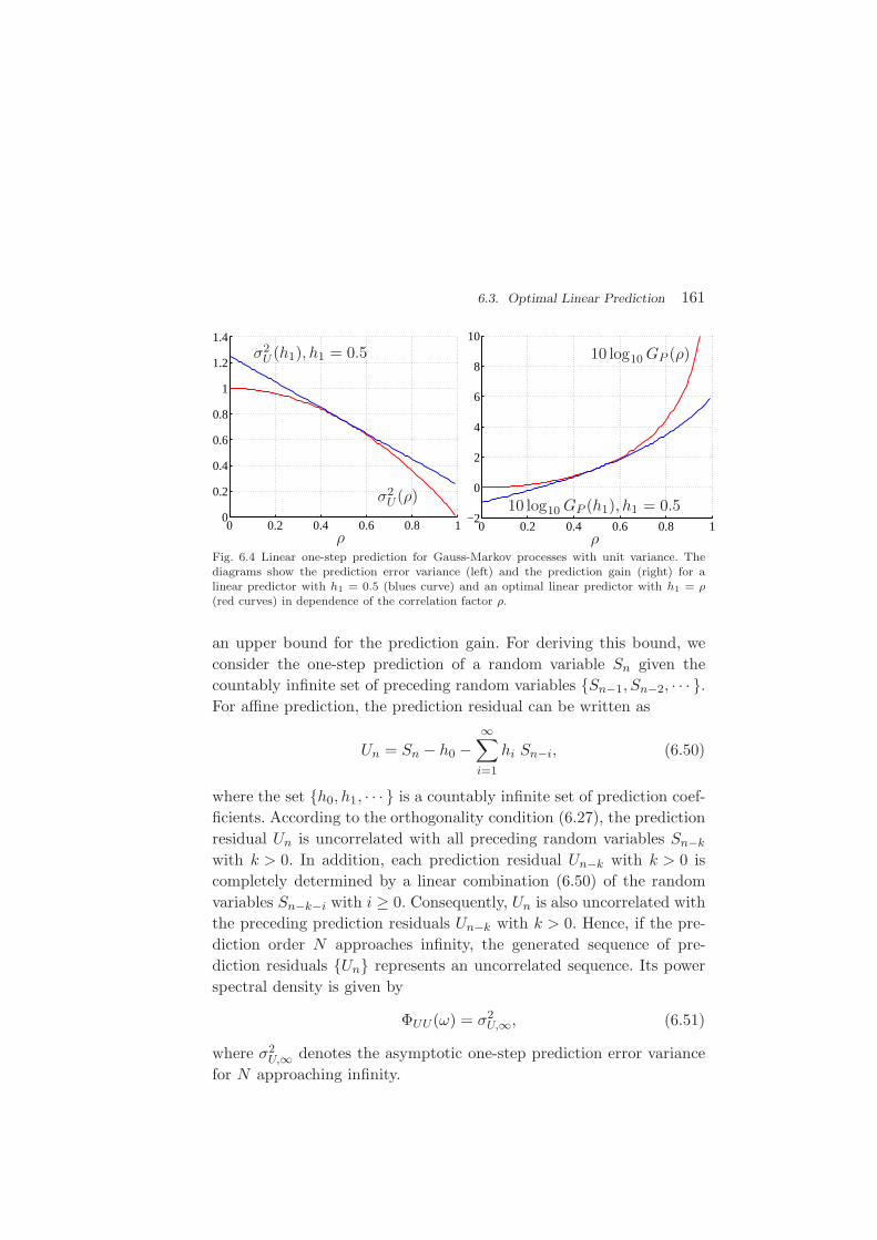
6.3. Optimal Linear Prediction 161
0 0.2 0.4 0.6 0.8 10
0.2
0.4
0.6
0.8
1
1.2
1.4
σ2U (ρ)
σ2U (h1), h1 = 0.5
ρ0 0.2 0.4 0.6 0.8 1
−2
0
2
4
6
8
10
10 log10 GP (ρ)
10 log10 GP (h1), h1 = 0.5
ρFig. 6.4 Linear one-step prediction for Gauss-Markov processes with unit variance. Thediagrams show the prediction error variance (left) and the prediction gain (right) for alinear predictor with h1 = 0.5 (blues curve) and an optimal linear predictor with h1 = ρ(red curves) in dependence of the correlation factor ρ.
an upper bound for the prediction gain. For deriving this bound, we
consider the one-step prediction of a random variable Sn given the
countably infinite set of preceding random variables {Sn−1, Sn−2, · · · }.For affine prediction, the prediction residual can be written as
Un = Sn − h0 −∞∑
i=1
hi Sn−i, (6.50)
where the set {h0, h1, · · · } is a countably infinite set of prediction coef-
ficients. According to the orthogonality condition (6.27), the prediction
residual Un is uncorrelated with all preceding random variables Sn−k
with k > 0. In addition, each prediction residual Un−k with k > 0 is
completely determined by a linear combination (6.50) of the random
variables Sn−k−i with i ≥ 0. Consequently, Un is also uncorrelated with
the preceding prediction residuals Un−k with k > 0. Hence, if the pre-
diction order N approaches infinity, the generated sequence of pre-
diction residuals {Un} represents an uncorrelated sequence. Its power
spectral density is given by
ΦUU(ω) = σ2U,∞, (6.51)
where σ2U,∞ denotes the asymptotic one-step prediction error variance
for N approaching infinity.
162 Predictive Coding
For deriving an expression for the asymptotic one-step prediction
error variance σ2U,∞, we restrict our considerations to zero-mean in-
put processes, for which the autocovariance matrix CN is equal to the
corresponding autocorrelation matrix RN , and first consider the limit
limN→∞
|CN |1N . (6.52)
Since the determinant of a N×N matrix is given by the product of its
eigenvalues ξ(N)i , with i = 0, 1, · · · , N − 1, we can write
limN→∞
|CN |1N = lim
N→∞
(N−1∏
i=0
ξ(N)i
)1N
= 2
(
limN→∞
N−1∑
i=0
1N
log2 ξ(N)i
)
. (6.53)
By applying Grenander and Szego’s theorem for sequences of Toeplitz
matrices (4.76), we obtain
limN→∞
|CN |1N = 2
12π
∫ π−π
log2 ΦSS(ω) dω, (6.54)
where ΦSS(ω) denotes the power spectral density of the input pro-
cess {Sn}. As a further consequence of the convergence of the limit in
(6.52), we can state
limN→∞
|CN+1|1
N+1
|CN |1N
= 1. (6.55)
According to (6.37), we can express the asymptotic one-step prediction
error variance σ2U,∞ by
σ2U,∞ = lim
N→∞|CN+1||CN |
= limN→∞
(
|CN+1|1
N+1
|CN |1N |CN |−
1N(N+1)
)N+1
. (6.56)
Applying (6.54) and (6.55) yields
σ2U,∞ = lim
N→∞|CN |
1N = 2
12π
∫ π−π log2 ΦSS(ω) dω. (6.57)
Hence, the asymptotic linear prediction gain for zero-mean input
sources is given by
G∞P =
σ2S
σ2U,∞
=12π
∫ π−π ΦSS(ω)dω
212π
∫ π−π log2 ΦSS(ω)dω
. (6.58)

6.4. Differential Pulse Code Modulation (DPCM) 163
0 0.2 0.4 0.6 0.8 10
5
10
15
20ΦSS(ω)
ρ = 0.9
ρ = 0.5ρ = 0
ω/π0 0.2 0.4 0.6 0.8 1
0
2
4
6
8
10
1210 log10 G∞
p (ρ)10.11 dB
7.21 dB
1.25 dB
ρ = 0.95
ρ = 0.9
ρ = 0.5
ρ
Fig. 6.5 Prediction gain for zero-mean Gauss-Markov sources: (left) Power spectral density;(right) Prediction gain.
It should be noted that for zero-mean AR(m) processes, such as
zero-mean Gauss-Markov processes, this asymptotic prediction gain is
already achieved by using optimal linear one-step predictors of a finite
order N ≥ m. As an example, we know from (4.77) to (4.79) that
1
2π
∫ π
−πlog2 ΦSS(ω) dω = log2
(σ2
S (1− ρ2))
(6.59)
for Gauss-Markov processes. This yields the asymptotic prediction gain
G∞P = 1/(1 − ρ2), which we have already derived for the optimal one-
step prediction in (6.45). This relationship can also be obtained by
inserting the expression (2.50) for the determinant |CN | into (6.57).
Fig. 6.5 illustrates the power spectral density and the prediction gain
for stationary zero-mean Gauss-Markov processes.
6.4 Differential Pulse Code Modulation (DPCM)
In the previous sections, we investigated the prediction and in par-
ticular the linear prediction of a random variable Sn using the values
of preceding random variables. We now consider the combination of
prediction and scalar quantization.
We first consider the case that the random variables of the input
process are predicted as discussed in the previous sections (i.e., using
the original values of preceding samples) and the resulting prediction
residuals are quantized. For the example of one-step prediction using

164 Predictive Coding
the directly preceding sample, we obtain the encoder reconstructions
S′n,e = U ′
n + Sn,e = Q(Sn −A(Sn−1)) + A(Sn−1). (6.60)
At the decoder side, however, we do not know the original sample
values. Here we must use the reconstructed values for deriving the
prediction values. The corresponding decoder reconstructions are given
by
S′n,d = U ′
n + Sn,d = Q(Sn −A(Sn−1)) + A(S′n−1,d). (6.61)
For such an open-loop predictive coding structure, the encoder and de-
coder reconstructions S′n,e and S′
n,d differ by P (Sn−1)− P (S′n−1,d). If
we use a recursive prediction structure as in the considered one-step
prediction, the differences between encoder and decoder reconstruc-
tions increase over time. This effect is also referred to as drift and can
only be avoided if the prediction at both encoder and decoder side uses
reconstructed samples.
Q! +!+!
ˆ S n
Sn
" S n
Un
" U n
-!
P!
ˆ S n
Q!
+!
+!Sn
" S n
Un
" U n
-!
P!
ˆ S n
Fig. 6.6 Closed-loop predictive coding: (left) Prediction structure using reconstructed sam-ples for forming the prediction signal; (right) DPCM structure.
The basic structure of a predictor that uses reconstructed sam-
ples S′n for forming the prediction signal is shown in the left block
diagram of Fig. 6.6. This structure is also referred to as closed-loop
predictive coding structure and is used in basically all video coding
applications. The closed-loop structure ensures that a decoder can ob-
tain the same reconstruction values as the encoder. By redrawing the
block diagram without changing the signal flow we obtain the structure
shown in the right block diagram of Fig. 6.6, which is also referred to
as differential pulse code modulation (DPCM).
If we decompose the quantizer Q in Fig. 6.6 into an encoder map-
ping α that maps the prediction residuals Un onto quantization in-
dexes In and a decoding mapping β that maps the quantization in-
dexes In onto reconstructed residuals U ′n and add a lossless coding γ

6.4. Differential Pulse Code Modulation (DPCM) 165
α
+
+Sn
′ S n
Un
′ U n
-
P
ˆ S n
β
In
+
γ γ -1 Bn
β
′ S n
P
′ U n
In
Bn
Channel
DPCM Encoder DPCM Decoder
ˆ S n
Fig. 6.7 Block diagram of a DPCM encoder and decoder.
for mapping the quantization indexes In onto codewords Bn, we obtain
the well-known structure of a DPCM encoder shown on the left side
of Fig. 6.7. The corresponding DPCM decoder is shown on the right
side of Fig. 6.7. It includes, the inverse lossless coding γ−1, the decoder
mapping β, and the predictor. If the codewords are transmitted over
an error-free channel, the reconstruction values at the decoder side are
identical to the reconstruction values at the encoder side, since the
mapping of the quantization indexes In to reconstructed values S′n is
the same in both encoder and decoder. The DPCM encoder contains
the DPCM decoder except for the inverse lossless coding γ−1.
6.4.1 Linear Prediction for DPCM
In sec. 6.3, we investigated optimal linear prediction of a random vari-
able Sn using original sample values of the past. However, in DPCM
coding, the prediction Sn for a random variable Sn must be generated
by a linear combination of the reconstructed values S′n of already coded
samples. If we consider linear one-step prediction using an observation
vector S′
n−1 = (S′n−1, · · · , S′
n−N )T that consists of the reconstruction
values of the N directly preceding samples, the prediction value Sn can
be written as
Sn =N∑
i=1
hi S′n−i =
K∑
i=1
hi (Sn−i+Qn−i) = hTN (SN
n−1+QNn−1), (6.62)
where Qn = U ′n − Un denotes the quantization error, hN is the vector
of prediction parameters, Sn−1 = (Sn−1, · · · , Sn−N )T is the vector of
the N original sample values that precede the current sample Sn to be

166 Predictive Coding
predicted, and Qn−1 = (Qn−1, · · · , Qn−N )T is the vector of the quan-
tization errors for the N preceding samples. The variance σ2U of the
prediction residual Un is given by
σ2U = E
{(Un−E{Un})2
}
= E{(
Sn−E{Sn} − hTN
(Sn−1−E{Sn−1}+ Qn−1−E
{Qn−1
} ))2}
= σ2S − 2hT
N c1 + hTN CN hN
− 2hTN E
{(Sn−E{Sn}
)(Qn−1−E
{Qn−1
} )}
− 2hTN E
{(Sn−1−E{Sn−1}
)(Qn−1−E
{Qn−1
} )T}
hN
+ hTN E
{(Qn−1−E
{Qn−1
} )(Qn−1−E
{Qn−1
} )T}
hN . (6.63)
The optimal prediction parameter vector hN does not only depend on
the autocovariances of the input process {Sn}, but also on the auto-
covariances of the quantization errors {Qn} and the cross-covariances
between the input process and the quantization errors. Thus, we need
to know the quantizer in order to design an optimal linear predictor.
But on the other hand, we also need to know the predictor parameters
for designing the quantizer. Thus, for designing a optimal DPCM coder
the predictor and quantizer have to be optimized jointly. Numerical al-
gorithms that iteratively optimize the predictor and quantizer based
on conjugate gradient numerical techniques are discussed in [8].
For high rates, the reconstructed samples S′n are a close approxima-
tion of the original samples Sn, and the optimal prediction parameter
vector hN for linear prediction using reconstructed sample values is vir-
tually identical to the optimal prediction parameter vector for linear
prediction using original sample values. In the following, we concentrate
on DPCM systems for which the linear prediction parameter vector is
optimized for a prediction using original sample values, but we note
that such DPCM systems are suboptimal for low rates.
One-Tap Prediction for Gauss-Markov Sources. As an impor-
tant example, we investigate the rate distortion efficiency of linear pre-
dictive coding for stationary Gauss-Markov sources,
Sn = Zn + µS (1− ρ) + ρSn−1. (6.64)

6.4. Differential Pulse Code Modulation (DPCM) 167
We have shown in sec. 6.3.2 that the optimal linear predictor using
original sample values is the one-tap predictor for which the prediction
coefficient h1 equal to the correlation coefficient ρ of the Gauss-Markov
process. If we use the same linear predictor with reconstructed samples,
the prediction Sn for a random variable Sn can be written as
Sn = h1 S′n−1 = ρ (Sn−1 + Qn−1), (6.65)
where Qn−1 = U ′n−1 − Un−1 denotes the quantization error. The pre-
diction residual Un is given by
Un = Sn − Sn = Zn + µS (1− ρ)− ρQn−1. (6.66)
For the prediction error variance σ2U , we obtain
σ2U = E
{(Un −E{Un})2
}= E
{(Zn − ρ (Qn−1 − E{Qn−1})
)2}
= σ2Z − 2 ρE{Zn (Qn−1 −E{Qn−1})}+ ρ2 σ2
Q, (6.67)
where σ2Z = E
{Z2
n
}denotes the variance of the innovation process {Zn}
and σ2Q = E
{(Qn − E{Qn})2
}denotes the variance of the quantization
errors. Since {Zn} is an iid process and thus Zn is independent of the
past quantization errors Qn−1, the middle term in (6.67) is equal to 0.
Furthermore, as shown in sec. 2.3.1, the variance σ2Z of the innovation
process is given by σ2S (1− ρ2). Hence, we obtain
σ2U = σ2
S (1− ρ2) + ρ2 σ2Q. (6.68)
We further note that the quantization error variance σ2Q represents the
distortion D of the DPCM quantizer and is a function of the rate R.
As explained in sec. 5.2.4, we can generally express the distortion rate
function of scalar quantizers by
D(R) = σ2Q(R) = σ2
U(R) g(R), (6.69)
where σ2U (R) represents the variance of the signal that is quantized. The
function g(R) represents the operational distortion rate function for
quantizing random variables that have the same distribution type as the
prediction residual Un, but unit variance. Consequently, the variance
of the prediction residual is given by
σ2U (R) = σ2
S
1− ρ2
1− ρ2 g(R). (6.70)

168 Predictive Coding
Using (6.69), we obtain the following operational distortion rate func-
tion for linear predictive coding of Gauss-Markov processes with a one-
tap predictor for which the prediction coefficient h1 is equal to the
correlation coefficient of the Gauss-Markov source,
D(R) = σ2S
1− ρ2
1− ρ2 g(R)g(R). (6.71)
By deriving the asymptote for g(R) approaching zero, we obtain the
following asymptotic operational distortion rate function for high rates,
D(R) = σ2S (1− ρ2) g(R). (6.72)
The function g(R) represents the operational distortion rate func-
tion for scalar quantization of random variables that have unit variance
and the same distribution type as the prediction residuals. It should be
mentioned that, even at high rates, the distribution of the prediction
residuals cannot be derived in a straightforward way, since it is de-
termined by a complicated process that includes linear prediction and
quantization. As a rule of thumb based on intuition, at high rates, the
reconstructed values S′n are a very close approximation of the original
samples Sn and thus the quantization errors Qn = S′n − Sn are very
small in comparison to the innovation Zn. Then, we can argue that
the prediction residuals Un given by (6.66) are nearly identical to the
innovation samples Zn and have thus nearly a Gaussian distribution.
Another reason for assuming a Gaussian model is the fact that Gaus-
sian sources are the most difficult to code among all processes with a
given autocovariance function. Using a Gaussian model for the predic-
tion residuals, we can replace g(R) in (6.72) by the high rate asymptote
for entropy-constrained quantization of Gaussian sources, which yields
the following high rate approximation of the operational distortion rate
function,
D(R) =π e
6σ2
S (1 − ρ2) 2−2R. (6.73)
Hence, under the intuitive assumption that the distribution of the
prediction residuals at high rates is nearly Gaussian, we obtain an
asymptotic operational distortion rate function for DPCM quanti-
zation of stationary Gauss-Markov processes at high rates that lies

6.4. Differential Pulse Code Modulation (DPCM) 169
1.53 dB or 0.25 bit per sample above the fundamental rate distor-
tion bound (4.119). The experimental results presented below indicate
that our intuitive assumption provides a useful approximation of the
operational distortion rate function for DPCM coding of stationary
Gauss-Markov processes at high rates.
Entropy-Constrained Lloyd Algorithm for DPCM. Even if
we use the optimal linear predictor for original sample values inside
the DPCM loop, the quantizer design algorithm is not straightforward,
since the distribution of the prediction residuals depends on the recon-
structed sample values and thus on the quantizer itself.
In order to provide some experimental results for DPCM quantiza-
tion of Gauss-Markov sources, we use a very simple ECSQ design in
combination with a given linear predictor. The vector of prediction pa-
rameters hN is given and only the entropy-constrained scalar quantizer
is designed. Given a sufficiently large training set {sn}, the quantizer
design algorithm can be stated as follows:
(1) Initialized the Lagrange multiplier λ with small value and
initialize all reconstructed samples s′n with the corresponding
original samples sn of the training set.
(2) Generate the residual samples using linear prediction given
the original and reconstructed samples sn and s′n.
(3) Design an entropy-constrained Lloyd quantizer as described
in sec. 5.2.2 given the value of λ and using the prediction
error sequence {un} as training set.
(4) Conduct the DPCM coding of the training set {sn} given the
linear predictor and the designed quantizer, which yields the
set of reconstructed samples {s′n}.(5) Increase λ by a small amount and start again with step 2.
The quantizer design algorithm starts with a small value of λ and
thus a high rate for which we can assume that reconstruction values
are nearly identical to the original sample values. In each iteration of
the algorithm, a quantizer is designed for a slightly larger value of λ
and thus a slightly lower rate by assuming that the optimal quantizer
170 Predictive Coding
design does not change significantly. By executing the algorithm, we
obtain a sequence of quantizers for different rates. It should however be
noted that the quantizer design inside a feedback loop is a complicated
problem. We noted that when the value of λ is changed too much from
one iteration to the next, the algorithm becomes unstable at low rates.
An alternative algorithm for designing predictive quantizers based on
conjugate gradient techniques can be found in [8].
Experimental Results for a Gauss-Markov Source. For provid-
ing experimental results, we considered the stationary Gauss-Markov
source with zero mean, unit variance, and a correlation factor of 0.9
that we have used as reference throughout this text. We have run the
entropy-constrained Lloyd algorithm for DPCM stated above and mea-
sured the prediction error variance σ2U , the distortion D, and the en-
tropy of the reconstructed sample values as measure for the transmis-
sion rate R. The results of the algorithm are compared to the distortion
rate function and to the derived functions for σ2U (R) and D(R) for sta-
tionary Gauss-Markov sources that are given in (6.70) and (6.71), re-
spectively. For the function g(R) we used the experimentally obtained
approximation (5.59) for Gaussian pdfs. It should be noted that the cor-
responding functional relationships σ2U (R) and D(R) are only a rough
approximation, since the distribution of the prediction residual Un can-
not be assumed to be Gaussian, at least not at low and medium rates.
In Fig. 6.8, the experimentally obtained data for DPCM coding with
entropy-constrained scalar quantization and for entropy-constrained
scalar quantization without prediction are compared to the derived
operational distortion rate functions using the approximation g(R) for
Gaussian sources given in (5.59) and the information rate distortion
function. For the shown experimental data and the derived operational
distortion rate functions, the rate has been measured as the entropy
of the quantizer output. The experimental data clearly indicate that
DPCM coding significantly increases the rate distortion efficiency for
sources with memory. Furthermore, we note that the derived oper-
ational distortion rate functions using the simple approximation for
g(R) represent suitable approximations for the experimentally obtained
data. At high rates, the measured difference between the experimental

6.4. Differential Pulse Code Modulation (DPCM) 171
0 1 2 3 40
5
10
15
20
25
30
space-filling gain: 1.53 dB
distortion ratefunction D(R)
EC-Lloy
d and DPCM
G∞P
=7.2
1 dB
Du(R) =σ2
U(R) g(R)
EC-Lloyd (no prediction)
Ds(R) = σ2S · g(R) bit rate [bit/sample]
SNR [dB]
Fig. 6.8 Linear predictive coding of a stationary Gauss-Markov source with unit varianceand a correlation factor of ρ = 0.9. The diagram compares the distortion rate efficiencyof ECSQ (without prediction) and ECSQ inside the prediction loop to the (information)distortion rate function D(R). The circles represent experimental data while the solid linesrepresent derived distortion rate functions. The rate is measured as the entropy of thequantizer output.
data for DPCM and the distortion rate bound is close to 1.53 dB, which
corresponds to the space-filling gain of vector quantization as the quan-
tizer dimension approaches infinity. This indicates that DPCM coding
of stationary Gauss-Markov sources can fully exploit the dependencies
inside the source at high rates and that the derived asymptotic oper-
ational distortion rate function (6.73) represents a reasonable approxi-
mation for distortion rate efficiency that can be obtained with DPCM
coding of stationary Gauss-Markov sources at high rates. At low rates,
the distance between the distortion rate bound and the obtained re-
sults for DPCM coding increases. A reason is that the variance σ2U of
the prediction residuals increases when the rate R is decreased, which
is illustrated in Fig. 6.9.
The DPCM gain can be defined as the ratio of the operational
distortion rate functions for scalar quantization and DPCM coding,
GDPCM(R) =σ2
S · gS(R)
σ2U · gU (R)
, (6.74)

172 Predictive Coding
0 1 2 3 40
0.2
0.4
0.6
0.8
1
σ2U(∞)
R [bit/symbol]= σ2S · (1− ρ2)
σ2U(R)
measurement
σ2U (R) = σ2
S · 1−ρ2
1−g(R) ρ2
Fig. 6.9 Variance of prediction residual σ2U as function of the bit rate for DPCM coding of
a Gauss-Markov source with unit variance and a correlation factor of ρ = 0.9. The circlesshow the experimental results while the solid line represents the derived approximation.The rate is measured as the entropy of the quantizer output.
where gS(R) and gU (R) represent the normalized operational distor-
tion rate functions for scalar quantization of the source signal and the
prediction residuals, respectively. At high rates and under our intu-
itive assumption that the prediction residuals are nearly Gaussian, the
normalized operational distortion rate function gU (R) for scalar quan-
tization of the prediction residuals becomes equal to the normalized
operational distortion rate function gS(R) for scalar quantization of the
original samples. Then, the asymptotic coding gain for DPCM coding
of stationary Gauss-Markov sources at high rates is approximately
G∞DPCM(R) =
σ2S
σ2U
=1
1− ρ2=
12π
∫ π−π ΦSS(ω)dω
212π
∫ π−π log2 ΦSS(ω)dω
. (6.75)
6.4.2 Adaptive Differential Pulse Code Modulation
So far we have discussed linear prediction and DPCM coding for sta-
tionary sources. However, the input signals in practical coding systems
are usually not stationary and thus a fixed predictor is not well suited.
For nonstationary signals the predictor needs to be adapted based on

6.4. Differential Pulse Code Modulation (DPCM) 173
local signal characteristics. The adaptation method is either signaled
from the sender to the receiver (forward adaptation) by side informa-
tion or simultaneously derived at both sides using a prescribed algo-
rithm (backward adaptation).
Forward Adaptive DPCM. A block diagram for a predictive
codec with forward adaptation is shown in Fig. 6.10. The encoder sends
new prediction coefficients to the decoder, which produces additional
bit rate. It is important to balance the increased bit rate for the adapta-
tion signal against the bit rate reduction resulting from improved pre-
diction. In practical codecs, the adaptation signal is send infrequently
at well-defined intervals. A typical choice in image and video coding is
to adapt the predictor on a block-by-block basis.
α
+
+Sn
′ S n
Un
′ U n
-
P
ˆ S n
β
In
+
γ γ -1 Bn
β
′ S n
P
′ U n
In
Bn
Channel
APF DPCM Encoder APF DPCM Decoder
ˆ S n
Buffer / APF APF Decoder
Fig. 6.10 Block diagram of a forward adaptive predictive codec.
Backward Adaptive DPCM. A block diagram for a predictive
codec with backward adaptation is shown in Fig. 6.11. The predic-
tion signal is derived from the previously decoded signal. It is advan-
tageous relative to forward adaptation in that no additional bit rate is
needed to signal the modifications of the predictor. Furthermore, back-
ward adaptation does not introduced any additional encoding-decoding
delay. The accuracy of the predictor is governed by the statistical prop-
erties of the source signal and the used adaptation algorithm. A draw-
back of backward adaptation is that the simultaneous computation of
the adaptation signal is its increased sensitivity to transmission errors.

174 Predictive Coding
α
+
+Sn
′ S n
Un
′ U n
-
P
ˆ S n
β
In
+
γ γ -1 Bn
β
′ S n
P
′ U n
In
Bn
Channel
APB DPCM Encoder APB DPCM Decoder
ˆ S n
APB APB
Fig. 6.11 Block diagram of a backward adaptive predictive codec.
6.5 Summary of Predictive Coding
In this chapter, we have discussed predictive coding. We introduced
the concept of prediction as a procedure of estimating the value of a
random variable based on already observed random variables. If the
efficiency of a predictor is measured by the mean squared prediction
error, the optimal prediction value is given by the conditional expecta-
tion of the random variable to be predicted given the observed random
variables. For particular important sources such as Gaussian sources
and autoregressive (AR) processes, the optimal predictor represents an
affine function of the observation vector. A method to generally reduce
the complexity of prediction is to constrain its structure to linear or
affine prediction. The difference between linear and affine prediction is
that the additional constant offset in affine prediction can compensate
for the mean of the input signal.
For stationary random processes, the optimal linear predictor is
given by the solution of the Yule-Walker equations and depends only
on the autocovariances of the source signal. If an optimal affine pre-
dictor is used, the resulting prediction residual is orthogonal to each of
the observed random variables. The optimal linear predictor for a sta-
tionary AR(m) process has m prediction coefficients, which are equal
to the model parameters of the input process. A stationary Gauss-

6.5. Summary of Predictive Coding 175
Markov process is a stationary AR(1) process and hence the optimal
linear predictor has a single prediction coefficient, which is equal to the
correlation coefficient of the Gauss-Markov process. It is important to
note that a non-matched predictor can increase the prediction error
variance relative to the signal variance.
Differential pulse code modulation (DPCM) is the dominant struc-
ture for the combination of prediction and scalar quantization. In
DPCM, the prediction is based on quantized samples. The combina-
tion of DPCM and entropy-constrained scalar quantization (ECSQ) has
been analyzed in great detail for the special case of stationary Gauss-
Markov processes. It has been shown that the prediction error variance
is dependent on the bit rate. The derived approximation for high rates,
which has been verified by experimental data, indicated that for sta-
tionary Gauss-Markov sources the combination of DPCM and ECSQ
achieves the shape and memory gain of vector quantization at high
rates.
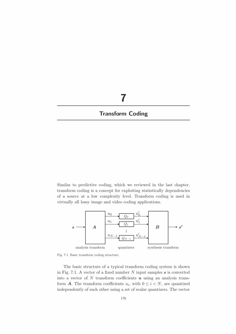
7
Transform Coding
Similar to predictive coding, which we reviewed in the last chapter,
transform coding is a concept for exploiting statistically dependencies
of a source at a low complexity level. Transform coding is used in
virtually all lossy image and video coding applications.
BA s′s
u0
u1
uN−1
u′0
u′1
u′N−1
Q0
Q1
QN−1
analysis transform synthesis transformquantizers
Fig. 7.1 Basic transform coding structure.
The basic structure of a typical transform coding system is shown
in Fig. 7.1. A vector of a fixed number N input samples s is converted
into a vector of N transform coefficients u using an analysis trans-
form A. The transform coefficients ui, with 0 ≤ i < N , are quantized
independently of each other using a set of scalar quantizers. The vector
176

177
of N reconstructed samples s′ is obtained by transforming the vector of
reconstructed transform coefficients u′ using a synthesis transform B.
In all practically used video coding systems, the analysis and syn-
thesis transforms A and B are orthogonal block transforms. The se-
quence of source samples {sn} is partitioned into vectors s of adjacent
samples and the transform coding consisting of an orthogonal analysis
transform, scalar quantization of the transform coefficients, and an or-
thogonal synthesis transform is independently applied to each vector
of samples. Since finally a vector s of sources samples is mapped to
a vector s′ of reconstructed samples, transform coding systems form
a particular class of vector quantizers. The benefit in comparison to
unconstrained vector quantization is that the imposed structural con-
straint allows implementations at a significantly lower complexity level.
The typical motivation for transform coding is the decorrelation and
energy concentration effect. Transforms are designed in a way that, for
typical input signals, the transform coefficients are much less correlated
than the original source samples and the signal energy is concentrated
in a few transform coefficients. As a result, the obtained transform co-
efficients have a different importance and simple scalar quantization
becomes more effective in the transform domain than in the original
signal space. Due to this effect, the memory advantage of vector quan-
tization can be exploited to a large extend for typical source signals.
Furthermore, by using entropy-constrained quantization for the trans-
form coefficients also the shape advantage can be obtained. In compar-
ison to unconstrained vector quantization, the rate distortion efficiency
is basically reduced by the space-filling advantage, which can only be
obtained by a significant increase in complexity.
For image and video coding applications, another advantage of
transform coding is that the quantization in the transform domain often
leads to an improvement of the subjective quality relative to a direct
quantization of the source samples with the same distortion, in partic-
ular for low rates. The reason is that the transform coefficients contain
information with different importance for the viewer and can there-
fore be treated differently. All perceptual distortion measures that are
known to provide reasonable results weight the distortion in the trans-
178 Transform Coding
form domain. The quantization of the transform coefficients can also
be designed in a way that perceptual criteria are taken into account.
In contrast to video coding, the transforms that are used in still im-
age coding are not restricted to the class of orthogonal block transforms.
Instead, transforms that do not process the input signal on a block-
by-block basis have been extensively studied and included into recent
image coding standards. One of these transforms is the so-called dis-
crete wavelet transform, which decomposes an image into components
that correspond to band-pass filtered and downsampled versions of the
image. Discrete wavelet transforms can be efficiently implemented us-
ing cascaded filter banks. Transform coding that is based on a discrete
wavelet transform is also referred to as subband coding and is for ex-
ample used in the JPEG 2000 standard [41, 72]. Another class of trans-
forms are the lapped block transforms, which are basically applied on
a block-by-block basis, but are characterized by basis functions that
overlap the block boundaries. As a result, the transform coefficients for
a block do not only depend on the samples inside the block, but also on
samples of neighboring blocks. The vector of reconstructed samples for
a block is obtained by transforming a vector that includes the trans-
form coefficients of the block and of neighboring blocks. A hierarchical
lapped transform with biorthogonal basis functions is included in the
latest image coding standard JPEG XR [42]. The typical motivation
for using wavelet transforms or lapped block transforms in image cod-
ing is that the nature of these transforms avoids the blocking artifacts
which are obtained by transform coding with block-based transforms
at low bit rates and are considered as one of the most disturbing coding
artifacts. In video coding, wavelet transforms and lapped block trans-
forms are rarely used due to the difficulties in efficiently combining
these transforms with inter-picture prediction techniques.
In this chapter, we discuss transform coding with orthogonal block
transforms, since this is the predominant transform coding structure in
video coding. For further information on transform coding in general,
the reader is referred to the tutorials [20] and [10]. An introduction to
wavelet transforms and subband coding is given in the tutorials [74,
76] and [77]. As a reference for lapped blocks transforms and their
application in image coding we recommend [62] and [53].

7.1. Structure of Transform Coding Systems 179
7.1 Structure of Transform Coding Systems
The basic structure of transform coding systems with block trans-
forms is shown in Fig. 7.1. If we split the scalar quantizers Qk, with
k = 0, . . . , N − 1, into an encoder mapping αk that converts the trans-
form coefficients into quantization indexes and a decoder mapping βk
that converts the quantization indexes into reconstructed transform
coefficients and additionally introduce a lossless coding γ for the quan-
tization indexes, we can decompose the transform coding system shown
in Fig. 7.1 into a transform encoder and a transform decoder as illus-
trated in Fig. 7.2.
γA bs
u0
u1
uN−1
i0
i1
iN−1
α0
α1
αN−1
analysis transform entropy coderencoder mapping
encoder
Bγ−1 s′b
i0
i1
iN−1
u′0
u′1
u′N−1
β0
β1
βN−1
entropy decoder synthesis transformdecoder mapping
decoder
Fig. 7.2 Encoder and decoder of a transform coding system.
In the transform encoder, the analysis transform converts a vector
s = (s0, · · · , sN−1)T of N source samples into a vector of N transform
coefficients u = (u0, · · · , uN−1)T . Each transform coefficient uk is then
mapped onto a quantization index ik using an encoder mapping αk.
The quantization indexes of all transform coefficients are coded using
a lossless mapping γ, resulting in a sequence of codewords b.

180 Transform Coding
In the transform decoder, the sequence of codewords b is mapped
to the set of quantization indexes ik using the inverse lossless map-
ping γ−1. The decoder mappings βk convert the quantization indexes ikinto reconstructed transform coefficients u′
k. The vector of N recon-
structed samples s′ = (s′0, · · · , s′N−1)T is obtained by transforming the
vector of N reconstructed transform coefficients u′ = (u′0, · · · , u′
N−1)T
using the synthesis transform.
7.2 Orthogonal Block Transforms
In the following discussion of transform coding, we restrict our consid-
erations to stationary sources and transform coding systems with the
following properties:
(1) Linear block transforms: The analysis and synthesis trans-
form are linear block transforms.
(2) Perfect reconstruction: The synthesis transform is the inverse
of the analysis transform.
(3) Orthonormal basis: The basis vectors of the analysis trans-
form form an orthonormal basis.
Linear Block Transforms. For linear block transforms of size N ,
each component of an N -dimensional output vector represents a linear
combination of the components of the N -dimensional input vector. A
linear block transform can be written as a matrix multiplication. The
analysis transform, which maps a vector of source samples s to a vector
of transform coefficients u, is given by
u = A s, (7.1)
where the matrix A is referred to as the analysis transform matrix.
Similarly, the synthesis transform, which maps a vector of reconstructed
transform coefficients u′ to a vector of reconstructed samples s′, can
be written as
s′ = B u′, (7.2)
where the matrix B represents the synthesis transform matrix.

7.2. Orthogonal Block Transforms 181
Perfect Reconstruction. The perfect reconstruction property
specifies that the synthesis transform matrix is the inverse of the anal-
ysis transform matrix, B=A−1. If the transform coefficients are not
quantized, i.e., if u′ = u, the vector of reconstructed samples is equal
to the vector of source samples,
s′ = B u = B A s = A−1 A s = s. (7.3)
If an invertible analysis transform A produces independent transform
coefficients and the component quantizers reconstruct the centroids of
the quantization intervals, the inverse of the analysis transform is the
optimal synthesis transform in the sense that it yields the minimum
distortion among all linear transforms given the coded transform coef-
ficients. It should, however, be noted that if these conditions are not
fulfilled, a synthesis transform B that is not equal to the inverse of the
analysis transform may reduce the distortion [20].
Orthonormal Basis. An analysis transform matrix A forms an or-
thonormal basis if its basis vectors given by the rows of the matrix
are orthogonal to each other and have the length 1. Matrices with this
property are referred to as unitary matrices. The corresponding trans-
form is said to be an orthogonal transform. The inverse of a unitary
matrix A is its conjugate transpose, A−1 =A†. A unitary matrix with
real entries is called an orthogonal matrix and its inverse is equal to
its transpose, A−1 =AT . For linear transform coding systems with the
perfect reconstruction property and orthogonal matrices, the synthesis
transform is given by
s′ = B u′ = AT u′. (7.4)
Unitary transform matrices are often desirable, because the mean
square error between a reconstruction and source vector can be min-
imized with independent scalar quantization of the transform coeffi-
cients. Furthermore, as we will show below, the distortion in the trans-
form domain is equal to the distortion in the original signal space.
In practical transform coding systems, it is usually sufficient to require
that the basis vectors are orthogonal to each other. The different norms
can be easily taken into account in the quantizer design.

182 Transform Coding
We can consider a linear analysis transform A as optimal if the
transform coding system consisting of the analysis transform A, op-
timal entropy-constrained scalar quantizers for the transform coeffi-
cients (which depend on the analysis transform), and the synthesis
transform B = A−1 yields a distortion for a particular given rate that
is not greater than the distortion that would be obtained with any
other transform at the same rate. In this respect, a unitary transform
is optimal for the MSE distortion measure if it produces independent
transform coefficients. Such a transform does, however, not exist for all
sources. Depending on the source signal, a non-unitary transform may
be superior [20, 13].
Properties of Orthogonal Block Transforms. An important
property of transform coding systems with the perfect reconstruction
property and unitary transforms is that the MSE distortion is preserved
in the transform domain. For the general case of complex transform ma-
trices, the MSE distortion between the reconstructed samples and the
source samples can be written as
dN (s, s′) =1
N(s− s′)† (s− s′)
=1
N
(A−1 u−B u′
)† (A−1 u−B u′
), (7.5)
where † denotes the conjugate transpose. With the properties of perfect
reconstruction and unitary transforms (B =A−1 =A†), we obtain
dN (s, s′) =1
N
(A† u−A† u′
)† (A† u−A† u′
)
=1
N(u− u′)† A A−1 (u− u′)
=1
N(u− u′)† (u− u′) = dN (u,u′). (7.6)
For the special case of orthogonal transform matrices, the conjugate
transposes in the above derivation can be replaced with the transposes,
which yields the same result. Scalar quantization that minimizes the
MSE distortion in the transform domain also minimizes the MSE dis-
tortion in the original signal space.

7.2. Orthogonal Block Transforms 183
Another important property for orthogonal transforms can be de-
rived by considering the autocovariance matrix for the random vec-
tors U of transform coefficients,
CUU = E{(U − E{U})(U − E{U})T
}. (7.7)
With U = AS and A−1 = AT , we obtain
CUU = E{A (S − E{S})(S − E{S})T AT
}= A CSS A−1, (7.8)
where CSS denotes the autocovariance matrix for the random vectors S
of original source samples. It is known from linear algebra that the
trace tr(X) of a matrix X is similarity-invariant,
tr(X) = tr(P X P−1), (7.9)
with P being an arbitrary invertible matrix. Since the trace of an auto-
covariance matrix is the sum of the variances of the vector components,
the arithmetic mean of the variances σ2i of the transform coefficients is
equal to the variance σ2S of the original samples,
1
N
N−1∑
i=0
σ2i = σ2
S . (7.10)
Geometrical Interpretation. An interpretation of the matrix mul-
tiplication in (7.2) is that the vector of reconstructed samples s′ is
represented as a linear combination of the columns of the synthesis
transform matrix B, which are also referred to as the basis vectors bk
of the synthesis transform. The weights in this linear combination are
given by the reconstructed transform coefficients u′k and we can write
s′ =
N−1∑
k=0
u′k bk = u′
0 b0 + u′1 b1 + · · · + u′
N−1 bN−1. (7.11)
Similarly, the original signal vector s is represented by a linear combi-
nation of the basis vectors ak of the inverse analysis transform, given
by the columns of A−1,
s =
N−1∑
k=0
uk ak = u0 a0 + u1 a1 + · · ·+ uN−1 aN−1, (7.12)

184 Transform Coding
where the weighting factors are the transform coefficients uk. If the
analysis transform matrix is orthogonal (A−1 = AT ), the columns
of A−1 are equal to the rows of A. Furthermore, the basis vectors ak are
orthogonal to each other and build a coordinate system with perpen-
dicular axes. Hence, there is a unique way to represent a signal vector s
in the new coordinate system given by the set of basis vectors {ak}.Each transform coefficient uk is given by the projection of the signal
vector s onto the corresponding basis vector ak, which can be written
as scalar product
uk = aTk s. (7.13)
Since the coordinate system spanned by the basis vectors has perpen-
dicular axes and the origin coincides with the origin of the signal co-
ordinate system, an orthogonal transform specifies rotations and re-
flections in the N -dimensional Euclidean space. If the perfect recon-
struction property (B = A−1) is fulfilled, the basis vectors bk of the
synthesis transform are equal to the basis vectors ak of the analysis
transform and the synthesis transform specifies the inverse rotations
and reflections of the analysis transform.
As a simple example, we consider the following orthogonal 2 × 2
synthesis matrix,
B =[b0 b1] =
1√2
[1 1
1 −1
]
. (7.14)
The analysis transform matrix A is given by the transpose of the syn-
thesis matrix, A = BT . The transform coefficients uk for a given signal
vector s are the scalar products of the signal vector s and the basis
vectors bk. For a signal vector s=[4, 3]T , we obtain
u0 = bT0 · s = (4 + 3)/
√2 = 3.5 ·
√2, (7.15)
u1 = bT1 · s = (4− 3)/
√2 = 0.5 ·
√2. (7.16)
The signal vector s is represented as a linear combination of the basis
vectors, where the weights are given by the transform coefficients,
s = u0 · b0 + u1 · b1[
4
3
]
= (3.5 ·√
2) · 1√2
[1
1
]
(0.5 ·√
2) · 1√2
[1
−1
]
. (7.17)

7.2. Orthogonal Block Transforms 185
As illustrated in Fig. 7.3, the coordinate system spanned by the basis
vectors b0 and b1 is rotated by 45 degrees relative to the original co-
ordinate system. The transform coefficients specify the projections of
the signal vector s onto the axes of the new coordinate system.
s0
s1
sb0
b1
u0 · b0
u1 · b1
Fig. 7.3 Geometric interpretation of an orthogonal 2 × 2 transform.
Fig. 7.4 illustrates the effect of a decorrelating orthogonal transform
on the example of the given 2 × 2 transform for stationary zero-mean
Gauss-Markov sources with unit variance and different correlation co-
efficients ρ. If the source samples are not correlated (ρ = 0), the trans-
form does not have any effect. But for correlated sources, the transform
rotates the distribution of the source vectors in a way that the primary
axes of the distribution are aligned with axes of the coordinate system
in the transform domain. For the example 2× 2 transform this has the
effect that the variance for one transform coefficient is minimized while
the variance of the other transform coefficient is maximized. The signal
energy is shifted toward the first transform coefficient U0.
In Fig. 7.5 the quantization cells for scalar quantization in the origi-
nal signal space are compared with the quantization cells for transform
coding. As discussed in Chapter 5, the effective quantization cells for
simple scalar quantization in the N -dimensional signal space are hy-
perrectangles that are aligned with the axes of the coordinate system
as illustrated in the left diagram of Fig. 7.5. For transform coding, the
quantization cells in the transform domain are hyperrectangles that
are aligned with the axes of the coordinate system of the transform
coefficients (middle diagram of Fig. 7.5). In the original signal space,

186 Transform Coding
−4 −2 0 2 4−4
−2
0
2
4ρ = 0
S0
S1
−4 −2 0 2 4−4
−2
0
2
4ρ = 0.5
S0
S1
−4 −2 0 2 4−4
−2
0
2
4ρ = 0.9
S0
S1
−4 −2 0 2 4−4
−2
0
2
4ρ = 0.95
S0
S1
−4 −2 0 2 4−4
−2
0
2
4
U0
U1
−4 −2 0 2 4−4
−2
0
2
4
U0
U1
−4 −2 0 2 4−4
−2
0
2
4
U0
U1
−4 −2 0 2 4−4
−2
0
2
4
U0
U1
Fig. 7.4 Effect of a decorrelating orthogonal transform on the example of the 2×2 transformgiven in (7.14) for stationary Gauss-Markov sources with zero mean, unit variance and dif-ferent correlation coefficients ρ: (top) distribution of sources vectors; (bottom) distributionof transform coefficient vectors.
the quantization cells are still hyperrectangles, but the grid of quantiza-
tion cells is rotated and aligned with the basis vectors of the orthogonal
transform as shown in the right diagram of Fig. 7.5. As a rough ap-
proximation, the required bit rate can be considered as proportional to
the number of quantization cells associated with appreciable probabili-
ties in the coordinate directions of the quantization grid. This indicates
that, for correlated sources, transform coding yields a higher rate dis-
tortion efficiency than scalar quantization in the original domain.
Fig. 7.5 Comparison of transform coding and scalar quantization in the original signal space:(left) source distribution and quantization cells for scalar quantization; (middle) distributionof transform coefficients and quantization cells in the transform domain; (right) sourcedistribution and quantization cells for transform coding in the original signal space.
7.3. Bit Allocation for Transform Coefficients 187
7.3 Bit Allocation for Transform Coefficients
Before we discuss decorrelating transforms in more detail, we analyze
the problem of bit allocation for transform coefficients. As mentioned
above, the transform coefficients have usually a different importance
and hence the overall rate distortion efficiency of a transform coding
system depends on a suitable distribution of the overall rate R among
the transform coefficients. A bit allocation is optimal if a given overall
rate R is distributed in a way that the resulting overall distortion D is
minimized. If we use the MSE distortion measure, the distortion in the
original signal space is equal to the distortion in the transform domain.
Hence, with Ri representing the component rates for the transform co-
efficients ui and Di(Ri) being the operational distortion rate functions
for the component quantizers, we want to minimize
D(R) =1
N
N−1∑
i=0
Di(Ri) subject to1
N
N−1∑
i=0
Ri = R. (7.18)
As has been discussed in sec. 5.2.2, the constrained optimization prob-
lem (7.18) can be reformulated as an unconstrained minimization of the
Lagrangian cost functional J = D + λR. If we assume that the oper-
ational distortion rate functions Di(Ri) for the component quantizers
are convex, the optimal rate allocation can be found by setting the
partial derivatives of the Lagrangian functional J with respect to the
component rates Ri equal to 0,
d
dRi
(
1
N
N∑
i=1
Di(Ri) +λ
N
N∑
i=1
Ri
)
=1
N
dDi(Ri)
dRi+
λ
N= 0, (7.19)
which yieldsd
dRiDi(Ri) = −λ = const. (7.20)
This so-called Pareto condition states that, for optimal bit allocation,
all component quantizers should be operated at equal slopes of their
operational distortion rate functions Di(Ri).
In sec. 5.2.4, we have shown that the operational distortion rate
function of scalar quantizers can be written as
Di(Ri) = σ2i · gi(Ri), (7.21)

188 Transform Coding
where σ2i is the variance of the input source and gi(Ri) is the oper-
ational distortion rate function for the normalized distribution with
unit variance. In general, it is justified to assume that gi(Ri) is a non-
negative, strictly convex function and has a continuous first derivative
g′i(Ri) with g′i(∞) = 0. Then, the Pareto condition yields
−σ2i g′i(Ri) = λ. (7.22)
As discussed in sec. 4.4, it has to be taken into account that the compo-
nent rate Ri for a particular transform coefficient cannot be negative.
If λ ≥ −σ2i g′i(0), the quantizer for the transform coefficient ui cannot
be operated at the given slope λ. In this case, it is optimal to set the
component rate Ri equal to zero. The overall distortion is minimized if
the overall rate is spent for coding only the transform coefficients with
−σ2i g′i(0) > λ. This yields the following bit allocation rule,
Ri =
{0 : −σ2
i g′i(0) ≤ λ
ηi
(
− λσ2
i
)
: −σ2i g
′i(0) > λ
, (7.23)
where ηi(·) denotes the inverse of the derivative g′i(·). Since g′i(Ri) is a
continuous strictly increasing function for Ri ≥ 0 with g′i(∞) = 0, the
inverse ηi(x) is a continuous strictly increasing function for the range
g′i(0) ≤ x ≤ 0 with ηi(f′i(0)) = 0 and ηi(0) =∞.
7.3.1 Approximation for Gaussian Sources
If the input signal has a Gaussian distribution, the distributions for all
transform coefficients are also Gaussian, since the signal for each trans-
form coefficient represents a linear combination of Gaussian sources.
Hence, we can assume that the operational distortion rate function for
all component quantizers is given by
Di(Ri) = σ2i · g(R), (7.24)
where g(R) represents the operational distortion rate function for
Gaussian sources with unit variance. In order to derive an approx-
imate formula for the optimal bit allocation, we assume that the
component quantizers are entropy-constrained scalar quantizers and
use the approximation (5.59) for g(R) that has been experimentally

7.3. Bit Allocation for Transform Coefficients 189
found for entropy-constrained scalar quantization of Gaussian sources
in sec. 5.2.4,
g(R) =ε2
aln(a · 2−2R + 1). (7.25)
The factor ε2 is equal to πe/6 and the model parameter a is approxi-
mately 0.9519. The derivative g′(R) and its inverse η(x) are given by
g′(R) = −ε2 · 2 ln 2
a + 22R, (7.26)
η(x) =1
2log2
(
−ε2 · 2 ln 2
x− a
)
. (7.27)
As stated above, for an optimal bit allocation, the component rate Ri
for a transform coefficient has to be set equal to 0, if
λ ≥ −σ2i g
′(0) = σ2i
ε2 · 2 ln 2
a + 1. (7.28)
With the parameter
θ = λa + 1
ε2 · 2 ln 2, (7.29)
we obtain the bit allocation rule
Ri(θ) =
{0 : θ ≥ σ2
i12 log2
(σ2
iθ (a + 1)− a
)
: θ < σ2i
. (7.30)
The resulting component distortions are given by
Di(θ) =
{σ2
i : θ ≥ σ2i
− ε2 ln 2a · σ2
i · log2
(
1− θσ2
i
aa+1
)
: θ < σ2i
. (7.31)
If the variances σ2i of the transform coefficients are known, the ap-
proximation of the operational distortion rate function for transform
coding of Gaussian sources with entropy-constrained scalar quantiza-
tion is given by the parametric formulation
R(θ) =1
N
N−1∑
i=0
Ri(θ), D(θ) =1
N
N−1∑
i=0
Di(θ), (7.32)
where R(θ) and D(θ) are specified by (7.30) and (7.31), respectively.
The approximation of the operational distortion rate function can be
calculated by varying the parameter θ in the range from 0 to σ2max,
with σ2max being the maximum variance of the transform coefficients.

190 Transform Coding
7.3.2 High-Rate Approximation
In the following, we assume that the overall rate R is high enough so
that all component quantizers are operated at high component rates Ri.
In sec. 5.2.3, we have shown that the asymptotic operational distortion
rate functions for scalar quantizers can be written as
Di(Ri) = ε2i σ2
i 2−2Ri , (7.33)
where the factor ε2i depends only on the type of the source distribution
and the used scalar quantizer. Using these high rate approximations
for the component quantizers, the Pareto condition becomes
d
dRiDi(Ri) = −2 ln 2 ε2
i σ2i−2Ri = −2 ln 2Di(Ri) = const. (7.34)
At high rates, an optimal bit allocation is obtained if all component
distortions Di are the same. Setting the component distortions Di equal
to the overall distortion D, yields
Ri(D) =1
2log2
(σ2
i ε2i
D
)
. (7.35)
For the overall operational rate distortion function, we obtain
R(D) =1
N
N−1∑
i=0
Ri(D) =1
2N
N−1∑
i=0
log2
(σ2
i ε2i
D
)
(7.36)
With the geometric means of the variances σ2i and the factors ǫ2
i ,
σ2 =
(N−1∏
i=0
σ2i
)1N
and ε2 =
(N−1∏
i=0
ε2i
)1N
, (7.37)
the asymptotic operational distortion rate function for high rates can
be written as
D(R) = ε2 · σ2 · 2−2R. (7.38)
It should be noted that this result can also be derived without using the
Pareto condition, which was obtained by calculus. Instead, we can use
the inequality of arithmetic and geometric means and derive the high
rate approximation similar to the rate distortion function for Gaussian
sources with memory in sec. 4.4.
7.4. The Karhunen Loeve Transform (KLT) 191
For Gaussian sources, all transform coefficients have a Gaussian
distribution (see sec. 7.3.1), and thus all factors ε2i are the same. If
entropy-constrained scalar quantizers are used, the factors ε2i are equal
to πe/6 (see sec. 5.2.3) and the asymptotic operational distortion rate
function for high rates is given by
D(R) =πe
6· σ2 · 2−2R. (7.39)
Transform Coding Gain. The effectiveness of a transform is often
specified by the transform coding gain, which is defined as the ratio
of the operational distortion rate functions for scalar quantization and
transform coding. At high rates, the transform coding gain is given by
GT =ε2S · σ2
S · 2−2R
ε2 · σ2 · 2−2R, (7.40)
where ε2S is the factor of the high rate approximation of the operational
distortion rate function for scalar quantization in the original signal
space and σ2S is the variance of the input signal.
By using the relationship (7.10), the high rate transform gain for
Gaussian sources can be expressed as the ratio of the arithmetic and
geometric mean of the transform coefficient variances,
GT =1N
∑N−1i=0 σ2
i
N
√∏N−1
i=0 σ2i
. (7.41)
The high rate transform gain for Gaussian sources is maximized if the
geometric mean is minimized. The transform that minimizes the geo-
metric mean is the Karhunen Loeve Transform, which will be discussed
in the next section.
7.4 The Karhunen Loeve Transform (KLT)
Due to its importance in the theoretical analysis of transform coding
we discuss the Karhunen Loeve Transform (KLT) in some detail in the
following. The KLT is an orthogonal transform that decorrelates the
vectors of input samples. The transform matrix A is dependent on the
statistics of the input signal.
192 Transform Coding
Let S represent the random vectors of original samples of a sta-
tionary input sources. The random vectors of transform coefficients are
given by U = A S and for the autocorrelation matrix of the transform
coefficients we obtain
RUU = E{U UT
}= E
{(AS)(AS)T
}= ARSSAT , (7.42)
where
RSS = E{SST
}(7.43)
denotes the autocorrelation matrix of the input process. To get uncor-
related transform coefficients, the orthogonal transform matrix A has
to be chosen in a way that the autocorrelation matrix RUU becomes a
diagonal matrix. Equation (7.42) can be slightly reformulated as
RSSAT = AT RSS . (7.44)
With bi representing the basis vectors of the synthesis transform, i.e.,
the column vectors of A−1 = AT and the row vectors of A, it becomes
obvious that RUU is a diagonal matrix if the eigenvector equation
RSS bi = ξi bi (7.45)
is fulfilled for all basis vectors bi. The eigenvalues ξi represents the ele-
ments rii on the main diagonal of the diagonal matrix RUU . The rows
of the transform matrix A are build by a set of unit-norm eigenvectors
of RSS that are orthogonal to each other. The autocorrelation matrix
for the transform coefficients RUU is a diagonal matrix with the eigen-
values of RSS on its main diagonal. The transform coefficient variances
σ2i are equal to the eigenvalues ξi of the autocorrelation matrix RSS.
A KLT exists for all sources, since symmetric matrices as the au-
tocorrelation matrix RSS are always orthogonally diagonizable. There
exist more than one KLT of any particular size N > 1 for all stationary
sources, because the rows of A can be multiplied by −1 or permuted
without influencing the orthogonality of A or the diagonal form of
RUU . If the eigenvalues of RSS are not distinct, there are additional
degrees of freedom for constructing KLT transform matrices. Numerical
methods for calculating the eigendecomposition RSS = AT diag(ξi)A
of real symmetric matrices RSS are the classical and the cyclic Jacobi
algorithm [43, 18].

7.4. The Karhunen Loeve Transform (KLT) 193
Nonstationary Sources. For nonstationary sources, transform cod-
ing with a single KLT transform matrix is suboptimal. Similar to the
predictor in predictive coding, the transform matrix should be adapted
based on the local signal statistics. The adaptation can be realized ei-
ther as forward adaptation or as backward adaptation. With forward
adaptive techniques, the transform matrix is estimated at the encoder
and an adaptation signal is transmitted as side information, which in-
creases the overall bit rate and usually introduces an additional delay.
In backward adaptive schemes, the transform matrix is simultaneously
estimated at the encoder and decoder side based on already coded
samples. Forward adaptive transform coding is discussed in [12] and
transform coding with backward adaptation is investigated in [21].
7.4.1 On the Optimality of the KLT
We showed that the KLT is an orthogonal transform that yields decor-
related transform coefficients. In the following, we show that the KLT
is also the orthogonal transform that maximizes the rate distortion
efficiency for stationary zero-mean Gaussian sources if optimal scalar
quantizers are used for quantizing the transform coefficients. The fol-
lowing proof was first delineated in [19].
We consider a transform coding system with an orthogonal N×N
analysis transform matrix A, the synthesis transform matrix B = AT ,
and scalar quantization of the transform coefficients. We further assume
that we use a set of scalar quantizers that are given by scaled versions
of a quantizer for unit variance for which the operational distortion
rate function is given by a nonincreasing function g(R). The decision
thresholds and reconstruction levels of the quantizers are scaled accord-
ing to the variances of the transform coefficients. Then, the operational
distortion rate function for each component quantizer is given by
Di(Ri) = σ2i · g(Ri), (7.46)
where σ2i denotes the variance of the corresponding transform coeffi-
cient (cp. sec. 5.2.4). It should be noted that such a setup is optimal
for Gaussian sources if the function g(R) is the operational distor-
tion rate function of an optimal scalar quantizer. The optimality of a

194 Transform Coding
quantizer may depend on the application. As an example, we could
consider entropy-constrained Lloyd quantizers as optimal if we assume
a lossless coding that achieves an average codeword length close to the
entropy. For Gaussian sources, the transform coefficients have also a
Gaussian distribution. The corresponding optimal component quantiz-
ers are scaled versions of the optimal quantizer for unit variance and
their operational distortion rate functions are given by (7.46).
We consider an arbitrary orthogonal transform matrix A0 and an
arbitrary bit allocation given by the vector b = (R0, · · ·RN−1)T with
∑N−1i=0 Ri = R. Starting with the given transform matrix A0 we apply
an iterative algorithm that generates a sequence of orthonormal trans-
form matrices {Ak}. The corresponding autocorrelation matrices are
given by R(Ak) = AkRSSATk with RSS denoting the autocorrelation
matrix of the source signal. The transform coefficient variances σ2i (Ak)
are the elements on the main diagonal of R(Ak) and the distortion rate
function for the transform coding system is given by
D(Ak, R) =N−1∑
i=0
σ2i (Ak) · g(Ri). (7.47)
Each iteration Ak 7→ Ak+1 shall consists of the following two steps:
(1) Consider the class of orthogonal reordering matrices {P },for which each row and column consists of a single one and
N − 1 zeros. The basis vectors given by the rows of Ak are
reordered by a multiplication with the reordering matrix P k
that minimizes the distortion rate function D(P kAk, R).
(2) Apply a Jacobi rotation1 Ak+1 = Qk(P kAk). The orthogo-
nal matrix Qk is determined in a way that the element rij
on a secondary diagonal of R(P kAk) that has the largest
absolute value becomes zero in R(Ak+1). Qk is an elemen-
tary rotation matrix. It is an identity matrix where the main
diagonal elements qii and qjj are replaced by a value cos ϕ
and the secondary diagonal elements qij and qji are replaced
by the values sinϕ and − sinϕ, respectively.
1 The classical Jacobi algorithm [43, 18] for determining the eigendecomposition of realsymmetric matrices consist of a sequence of Jacobi rotations.

7.4. The Karhunen Loeve Transform (KLT) 195
It is obvious that the reordering step does not increase the distor-
tion, i.e., D(P kAk, R) ≤ D(Ak, R). Furthermore, for each pair of vari-
ances σ2i (P kAk) ≥ σ2
j (P kAk), it implies g(Ri) ≤ g(Rj); otherwise, the
distortion D(P kAk, R) could be decreased by switching the i-th and
j-th row of the matrix P kAk. A Jacobi rotation that zeros the el-
ement rij of the autocorrelation matrix R(P kAk) in R(Ak+1) does
only change the variances for the i-th and j-th transform coefficient. If
σ2i (P kAk) ≥ σ2
j (P kAk), the variances are modified according to
σ2i (Ak+1) = σ2
i (P kAk) + δ(P kAk), (7.48)
σ2j (Ak+1) = σ2
j (P kAk)− δ(P kAk), (7.49)
with
δ(P kAk) =2r2
ij
(rii − rjj) +√
(rii − rjj)2 + 4r2ij
≥ 0, (7.50)
and rij being the elements of the matrix R(P kAk). The overall distor-
tion for the transform matrix Ak+1 will never become smaller than the
overall distortion for the transform matrix Ak,
D(Ak+1, R) =N−1∑
i=0
σ2i (Ak+1) · g(Ri)
= D(P kAk, R) + δ(P kAk) · (g(Ri)− g(Rj))
≤ D(P kAk, R) ≤ D(Ak, R). (7.51)
The described algorithm represents the classical Jacobi algorithm
[43, 18] with additional reordering steps. The reordering steps do not
affect the basis vectors of the transform (rows of the matrices Ak), but
only their ordering. As the number of iteration steps approaches infin-
ity, the transform matrix Ak approaches the transform matrix of a KLT
and the autocorrelation matrix R(Ak) approaches a diagonal matrix.
Hence, for each possible bit allocation, there exists a KLT that gives an
overall distortion that is smaller than or equal to the distortion for any
other orthogonal transform. While the basis vectors of the transform
are determined by the source signal, their ordering is determined by
the relative ordering of the partial rates Ri inside the bit allocation
vector b and the normalized operational distortion rate function g(Ri).

196 Transform Coding
We have shown that the KLT is the orthogonal transform that min-
imizes the distortion for a set of scalar quantizers that represent scaled
versions of a given quantizer for unit variance. In particular, the KLT is
the optimal transform for Gaussian sources if optimal scalar quantizers
are used [19]. The KLT produces decorrelated transform coefficients.
However, decorrelation does not necessarily imply independence. For
non-Gaussian sources, other orthogonal transforms or nonorthogonal
transforms can be superior with respect to the coding efficiency [20, 13].
Example for a Gauss-Markov Process. As an example, we con-
sider the 3×3 KLT for a stationary Gauss-Markov process with zero
mean, unit variance, and a correlation coefficient of ρ = 0.9. We assume
a bit allocation vector b = [5, 3, 2] and consider entropy-constrained
scalar quantizers. We further assume that the high-rate approximation
of the operational distortion rate function Di(Ri) = ε2σ2i 2
−2Ri with
ε2 =πe/6 is valid for the considered rates. The initial transform matrix
A0 shall be the matrix of the DCT-II transform, which we will later
introduce in sec. 7.5.3. The autocorrelation matrix RSS and the initial
transform matrix A0 are given by
Rs =
[1 0.9 0.81
0.9 1 0.90.81 0.9 1
]
, A0 =
[0.5774 0.5774 0.57740.7071 0 −0.70710.4082 −0.8165 0.4082
]
.
(7.52)
For the transform coefficients, we obtain the autocorrelation matrix
R(A0) =
[2.74 0 −0.0424
0 0.19 0−0.0424 0 0.07
]
. (7.53)
The distortion D(A0, R) for the initial transform is equal to 0.01426.
We now investigate the effect of the first iteration of the algorithm
described above. For the given relative ordering in the bit allocation
vector b, the optimal reordering matrix P 0 is the identity matrix. The
Jacobi rotation matrix Q0 and the resulting new transform matrix A1
are given by
Q0 =
[0.9999 0 −0.0159
0 1 00.0159 0 0.9999
]
, A1 =
[0.5708 0.5902 0.57080.7071 0 −0.70710.4174 −0.8072 0.4174
]
.
(7.54)

7.4. The Karhunen Loeve Transform (KLT) 197
The parameter δ(P 0A0) is equal to 0.000674. The distortion D(A1, R)
is equal to 0.01420. In comparison to the distortion for the initial trans-
form matrix A0, it has been reduced by about 0.018 dB. The autocor-
relation matrix R(A1) for the new transform coefficients is given by
R(A1) =
[2.7407 0 0
0 0.19 00 0 0.0693
]
. (7.55)
The autocorrelation matrix has already become a diagonal matrix after
the first iteration. The transform given by A1 represents a KLT for the
given source signal.
7.4.2 Asymptotic Operational Distortion Rate Function
In sec. 7.3.2, we considered the bit allocation for transform coding at
high rates. An optimal bit allocation results in constant component
distortions Di, which are equal to the overall distortion D. By using
the high rate approximation Di(Ri) = ε2i σ2
i 2−2Ri for the operational
distortion rate function of the component quantizers, we derived the
overall operational distortion rate function given in (7.36). For Gaus-
sian sources and entropy-constrained scalar quantization, all param-
eters ε2i are equal to ε = πe/6. And if we use a KLT of size N as
transform matrix, the transform coefficient variances σ2i are equal to
the eigenvalues ξ(N)i of the N -th order autocorrelation matrix RN for
the input process. Hence, for Gaussian sources and a transform coding
system that consists of a KLT of size N and entropy-constrained scalar
quantizers for the transform coefficients, the high rate approximation
for the overall distortion rate function can be written as
DN (R) =π e
6
(N−1∏
i=0
ξ(N)i
) 1N
2−2R. (7.56)
The larger we choose the transform size N of the KLT, the more the
samples of the input source are decorrelated. For deriving a bound for
the operational distortion rate function at high rates, we consider the
limit for N approaching infinity. By applying Grenander and Szego’s
theorem (4.76) for sequences of Toeplitz matrices, the limit of (7.56) for
N approaching infinity can be reformulated using the power spectral

198 Transform Coding
density ΦSS(ω) of the input source. For Gaussian sources, the asymp-
totic operational distortion rate function for high rates and large trans-
form dimensions is given by
D∞(R) =πe
6· 2 1
2π
∫ π−π log2ΦSS(ω) dω · 2−2R. (7.57)
A comparison with the Shannon lower bound (4.77) for zero-mean
Gaussian sources shows that the asymptotic operational distortion rate
function lies 1.53 dB or 0.25 bit per sample above this fundamental
bound. The difference is equal to the space-filling advantage of high-
dimensional vector quantization. For zero-mean Gaussian sources and
high rates, the memory and shape advantage of vector quantization can
be completely exploited using a high-dimensional transform coding.
By using the relationship σ2S = 1
2π
∫ π−π ΦSS(ω)dω for the variance of
the input source, the asymptotic transform coding gain for zero-mean
Gaussian sources can be expressed as the ratio of the arithmetic and
geometric means of the power spectral density,
G∞T =
ε2σ2S2−2R
D∞(R)=
12π
∫ π−π ΦSS(ω)dω
212π
∫ π−π log2 ΦSS(ω)dω
(7.58)
The asymptotic transform coding gain at high rates is identical to the
approximation for the DPCM coding gain at high rates (6.75).
Zero-Mean Gauss-Markov Sources. We now consider the special
case of zero-mean Gauss-Markov sources. The product of the eigenval-
ues ξ(N)i of a matrix RN is always equal to the determinant |RN | of
the matrix. And for zero-mean sources, the N -th order autocorrela-
tion matrix RN is equal to the N -th order autocovariance matrix CN .
Hence, we can replace the product of the eigenvalues in (7.56) with
the determinant |CN | of the N -th order autocovariance matrix. Fur-
thermore, for Gauss-Markov sources, the determinant of the N -th or-
der autocovariance matrix can be expressed according to (2.50). Using
these relationships, the operational distortion rate function for zero-
mean Gauss-Markov sources and a transform coding system with an
N -dimensional KLT and entropy-constrained component quantizers is
given by
DN (R) =π e
6σ2
S (1− ρ2)N−1
N 2−2R, (7.59)

7.4. The Karhunen Loeve Transform (KLT) 199
where σ2S and ρ denote the variance and the correlation coefficient of
the input source. For the corresponding transform gain, we obtain
GNT = (1− ρ2)
1−NN . (7.60)
The asymptotic operational distortion rate function and the asymptotic
transform gain for high rates and N approaching infinity are given by
D∞(R) =π e
6σ2
S (1− ρ2) 2−2R, G∞T =
1
(1− ρ2). (7.61)
7.4.3 Performance for Gauss-Markov Sources
For demonstrating the effectiveness of transform coding for correlated
input sources, we used a Gauss-Markov source with zero mean, unit
variance, and a correlation coefficient of ρ = 0.9 and compared the
rate distortion efficiency of transform coding with KLT’s of different
sizes N and entropy-constrained scalar quantization (ECSQ) with the
fundamental rate distortion bound and the rate distortion efficiency
for ECSQ of the input samples. The experimentally obtained data and
0 1 2 3 40
5
10
15
20
25
30space-filling gain: 1.53 dB
distortion ratefunction D(R)
G∞T
=7.2
1 dB
EC-Lloyd (no transform)
bit rate [bit/sample]
SNR [dB]KLT+ECSQ with N →∞
N = 16N = 8N = 4N = 2
Fig. 7.6 Transform coding of a Gauss-Markov source with zero mean, unit variance, and acorrelation coefficient of ρ = 0.9. The diagram compares the efficiency of direct ECSQ andtransform coding with ECSQ to the distortion rate function D(R). The circles representexperimental data while the solid lines represent calculated curves. The rate is measuredas the average of the entropies for the outputs of the component quantizers.
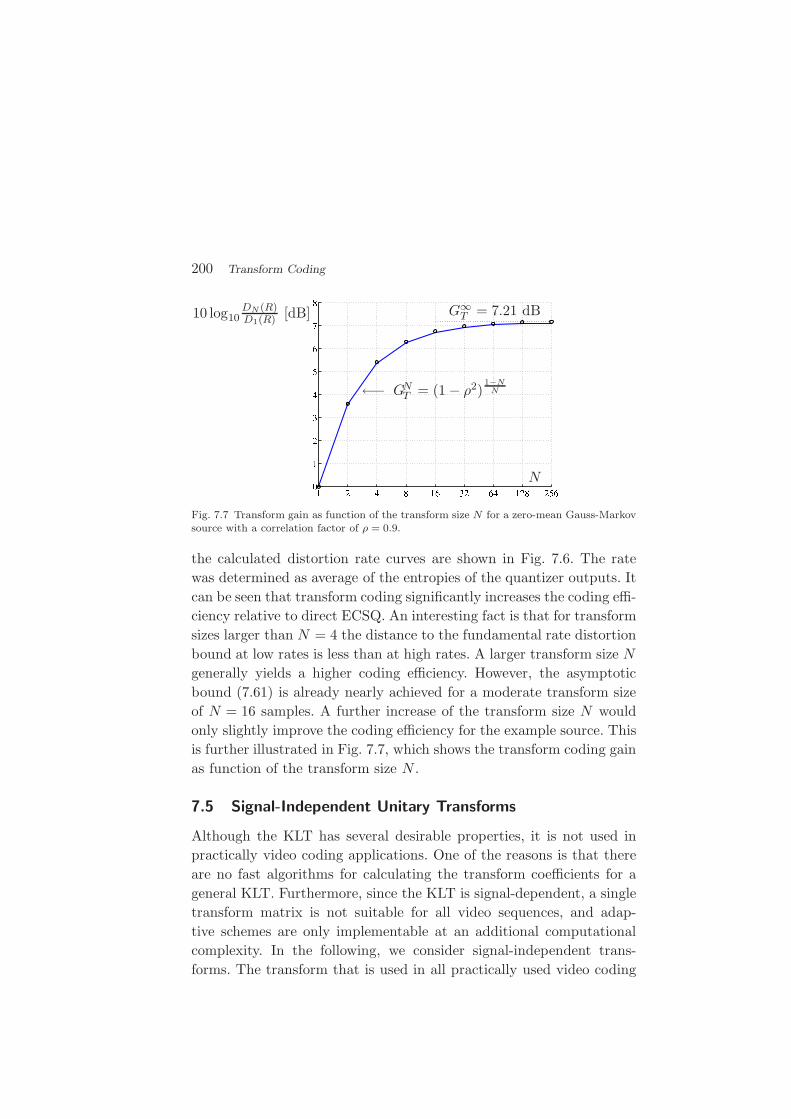
200 Transform Coding
G∞T = 7.21 dB
N
10 log10DN (R)D1(R) [dB]
←− GNT = (1− ρ2)
1−NN
Fig. 7.7 Transform gain as function of the transform size N for a zero-mean Gauss-Markovsource with a correlation factor of ρ = 0.9.
the calculated distortion rate curves are shown in Fig. 7.6. The rate
was determined as average of the entropies of the quantizer outputs. It
can be seen that transform coding significantly increases the coding effi-
ciency relative to direct ECSQ. An interesting fact is that for transform
sizes larger than N = 4 the distance to the fundamental rate distortion
bound at low rates is less than at high rates. A larger transform size N
generally yields a higher coding efficiency. However, the asymptotic
bound (7.61) is already nearly achieved for a moderate transform size
of N = 16 samples. A further increase of the transform size N would
only slightly improve the coding efficiency for the example source. This
is further illustrated in Fig. 7.7, which shows the transform coding gain
as function of the transform size N .
7.5 Signal-Independent Unitary Transforms
Although the KLT has several desirable properties, it is not used in
practically video coding applications. One of the reasons is that there
are no fast algorithms for calculating the transform coefficients for a
general KLT. Furthermore, since the KLT is signal-dependent, a single
transform matrix is not suitable for all video sequences, and adap-
tive schemes are only implementable at an additional computational
complexity. In the following, we consider signal-independent trans-
forms. The transform that is used in all practically used video coding

7.5. Signal-Independent Unitary Transforms 201
schemes is the discrete cosine transform (DCT), which will be discussed
in sec. 7.5.3. In addition, we will briefly review the Walsh-Hadamard
transform and, for motivating the DCT, the discrete Fourier transform.
7.5.1 The Walsh-Hadamard Transform (WHT)
The Walsh-Hadamard transform is a very simple orthogonal transform
that can be implemented using only additions and a final scaling. For
transform sizes N that represent positive integer power of 2, the trans-
form matrix AN is recursively defined by
AN =1√2
[AN/2 AN/2
AN/2 −AN/2
]
with A1 = [1]. (7.62)
When ignoring the constant normalization factor, the Hadamard trans-
form matrices only consist of entries equal to 1 and −1 and, hence, the
transform coefficients can be calculated very efficiently. However, due to
its piecewise-constant basis vectors, the Hadamard transform produces
subjectively disturbing artifacts if it is combined with strong quanti-
zation of the transform coefficients. In video coding, the Hadamard
transform is only used for some special purposes. An example is the
second-level transform for chroma coefficients in H.264/AVC [36]
7.5.2 The Discrete Fourier Transform (DFT)
One of the most important transforms in communications engineering
and signal processing is the Fourier transform. For discrete-time signals
of a finite length N , the discrete Fourier transform (DFT) is given by
u[k] =1√N
N−1∑
n=0
s[n] e−j 2πknN , (7.63)
where s[n], with 0 ≤ n < N , and u[k], with 0 ≤ k < N , represent the
components of the signal vector s and the vector of transform coeffi-
cients u, respectively, and j is the imaginary unit. The inverse DFT is
given by
s[n] =1√N
N−1∑
k=0
u[k] ej 2πknN . (7.64)
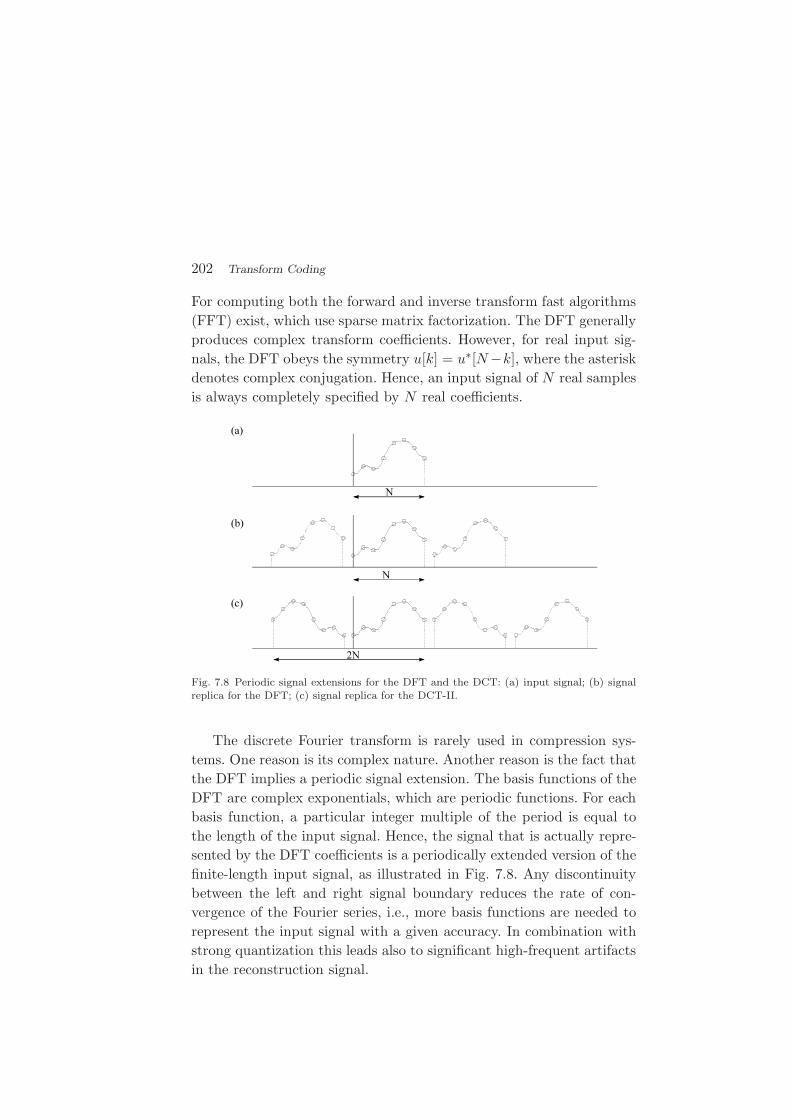
202 Transform Coding
For computing both the forward and inverse transform fast algorithms
(FFT) exist, which use sparse matrix factorization. The DFT generally
produces complex transform coefficients. However, for real input sig-
nals, the DFT obeys the symmetry u[k] = u∗[N−k], where the asterisk
denotes complex conjugation. Hence, an input signal of N real samples
is always completely specified by N real coefficients.
Fig. 7.8 Periodic signal extensions for the DFT and the DCT: (a) input signal; (b) signalreplica for the DFT; (c) signal replica for the DCT-II.
The discrete Fourier transform is rarely used in compression sys-
tems. One reason is its complex nature. Another reason is the fact that
the DFT implies a periodic signal extension. The basis functions of the
DFT are complex exponentials, which are periodic functions. For each
basis function, a particular integer multiple of the period is equal to
the length of the input signal. Hence, the signal that is actually repre-
sented by the DFT coefficients is a periodically extended version of the
finite-length input signal, as illustrated in Fig. 7.8. Any discontinuity
between the left and right signal boundary reduces the rate of con-
vergence of the Fourier series, i.e., more basis functions are needed to
represent the input signal with a given accuracy. In combination with
strong quantization this leads also to significant high-frequent artifacts
in the reconstruction signal.

7.5. Signal-Independent Unitary Transforms 203
7.5.3 The Discrete Cosine Transform (DCT)
The magnitudes of the high-frequency DFT coefficients can be reduced
by symmetrically extending the finite-length input signal at its bound-
aries and applying a DFT of approximately double size. If the extended
signal is mirror symmetric around the origin, the imaginary sine terms
get eliminated and only real cosine terms remain. Such a transform is
denoted as discrete cosine transform (DCT). There are several DCT’s,
which differ in the introduced signal symmetry. The most commonly
used form is the DCT-II, which can be derived by introducing mir-
ror symmetry with sample repetition at both boundaries as illustrated
in Fig. 7.8(c). For obtaining mirror symmetry around the origin, the
signal has to be shifted by half a sample. The signal s′ of 2N samples
that is actually transformed using the DFT is given by
s′[n] =
{s[n− 1/2] : 0 ≤ n < N
s[2N − n− 3/2] : N ≤ n < 2N. (7.65)
For the transform coefficients u′[k], we obtain
u′[k] =1√2N
2N−1∑
i=0
s′[i]e−j 2πkn2N
=1√2N
N−1∑
n=0
s[n− 1/2](
e−j πN
kn + e−j πN
k(2N−n−1))
=1√2N
N−1∑
n=0
s[n](
e−j πN
k(n+ 12) + ej π
Nk(n+ 1
2))
=
√
2
N
N−1∑
n=0
s[n] cos
(π
Nk
(
n +1
2
))
. (7.66)
In order to get an orthogonal transform, the DC coefficient u′[0] has to
be divided by√
2. The forward transform of the DCT-II is given by
u[k] =
N−1∑
n=0
s[n] αk cos
(π
Nk
(
n +1
2
))
, (7.67)
with
αn =
√
1
N·{
1 : n = 0√2 : n > 0
. (7.68)
204 Transform Coding
The inverse transform is given by
s[n] =N−1∑
k=0
u[k] · αk · cos(
π
Nk
(
n +1
2
))
. (7.69)
The DCT-II is the most commonly used transform in image
and video coding application. It is included in the following coding
standards: JPEG [38], H.261 [35], H.262/MPEG-2 [39], H.263 [36],
and MPEG-4 [31]. Although, the most recent video coding standard
H.264/AVC [36] does not include a DCT as discussed above, it in-
cludes an integer approximation of the DCT that has similar proper-
ties, but can be implemented more efficiently and does not cause an
accumulation of rounding errors inside the motion-compensation loop.
The justification for the wide usage of the DCT includes the following
points:
• The DCT does not depend on the input signal.
• There are fast algorithms for computing the forward and
inverse transform.
• The DCT can be extended to two (or more) dimensions in a
separable way.
• The DCT is a good approximation of the KLT for highly
correlated Gauss-Markov sources (see below).
Comparison of DCT and KLT. In contrast to the KLT, the basis
vectors of the DCT are independent of the input source and there exist
fast algorithms for computing the forward and inverse transforms. For
zero-mean Gauss-Markov sources with large correlation coefficients ρ,
the DCT-II basis vectors are a good approximation of the eigenvec-
tors of the autocorrelation matrix RSS . If we neglect possible multi-
plications with −1, the basis vectors of the KLT for zero-mean Gauss-
Markov sources approach the DCT-II basis vectors as the correlation
coefficient ρ approaches one [2]. This is illustrated in Fig. 7.9. On the
left side of this figure, the basis vectors of a KLT for zero-mean Gauss-
Markov sources with a correlation coefficient of ρ = 0.9 are compared
with the basis vectors of the DCT-II. On the right side of Fig. 7.9,
the mean square difference δ(ρ) between the transform matrix of the
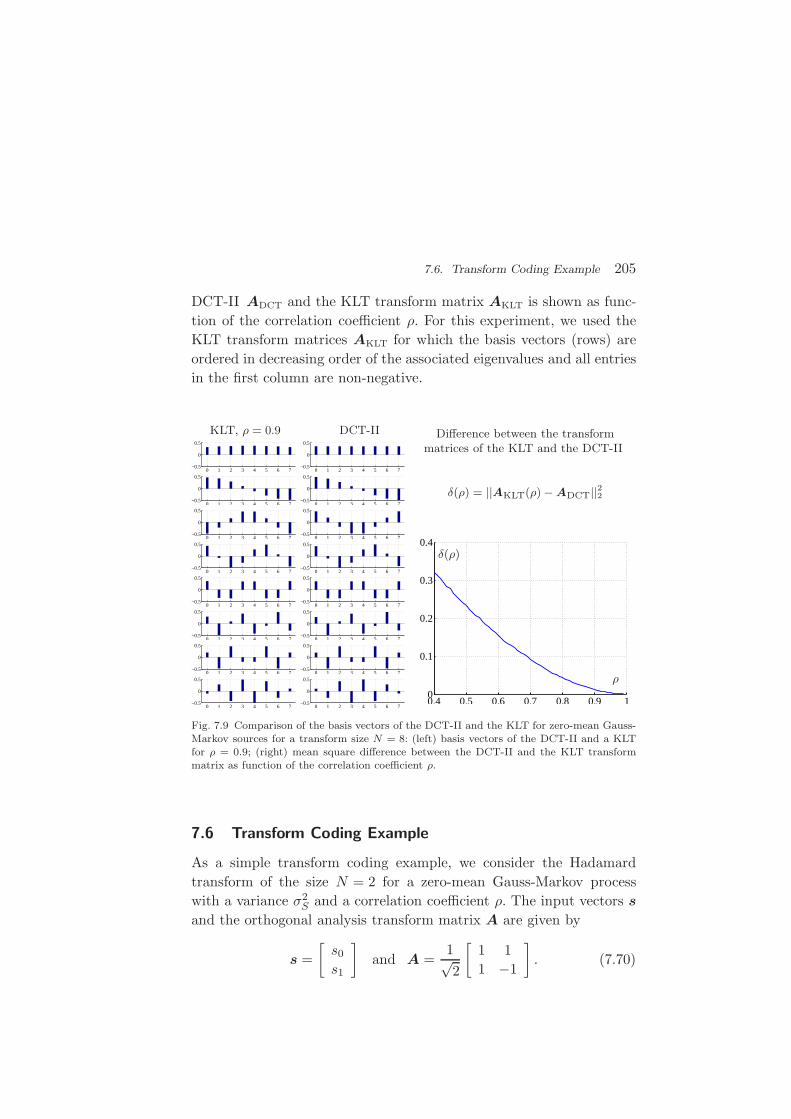
7.6. Transform Coding Example 205
DCT-II ADCT and the KLT transform matrix AKLT is shown as func-
tion of the correlation coefficient ρ. For this experiment, we used the
KLT transform matrices AKLT for which the basis vectors (rows) are
ordered in decreasing order of the associated eigenvalues and all entries
in the first column are non-negative.
0 1 2 3 4 5 6 7−0.5
0
0.5
0 1 2 3 4 5 6 7−0.5
0
0.5
0 1 2 3 4 5 6 7−0.5
0
0.5
0 1 2 3 4 5 6 7−0.5
0
0.5
0 1 2 3 4 5 6 7−0.5
0
0.5
0 1 2 3 4 5 6 7−0.5
0
0.5
0 1 2 3 4 5 6 7−0.5
0
0.5
0 1 2 3 4 5 6 7−0.5
0
0.5
0 1 2 3 4 5 6 7−0.5
0
0.5
0 1 2 3 4 5 6 7−0.5
0
0.5
0 1 2 3 4 5 6 7−0.5
0
0.5
0 1 2 3 4 5 6 7−0.5
0
0.5
0 1 2 3 4 5 6 7−0.5
0
0.5
0 1 2 3 4 5 6 7−0.5
0
0.5
0 1 2 3 4 5 6 7−0.5
0
0.5
0 1 2 3 4 5 6 7−0.5
0
0.5
KLT, ρ = 0.9 DCT-II Difference between the transformmatrices of the KLT and the DCT-II
δ(ρ) = ||AKLT(ρ) − ADCT||22
0.4 0.5 0.6 0.7 0.8 0.9 10
0.1
0.2
0.3
0.4δ(ρ)
ρ
Fig. 7.9 Comparison of the basis vectors of the DCT-II and the KLT for zero-mean Gauss-Markov sources for a transform size N = 8: (left) basis vectors of the DCT-II and a KLTfor ρ = 0.9; (right) mean square difference between the DCT-II and the KLT transformmatrix as function of the correlation coefficient ρ.
7.6 Transform Coding Example
As a simple transform coding example, we consider the Hadamard
transform of the size N = 2 for a zero-mean Gauss-Markov process
with a variance σ2S and a correlation coefficient ρ. The input vectors s
and the orthogonal analysis transform matrix A are given by
s =
[s0
s1
]
and A =1√2
[1 1
1 −1
]
. (7.70)

206 Transform Coding
The analysis transform
u =
[u0
u1
]
= As =1√2
[1 1
1 −1
] [s0
s1
]
(7.71)
yields the transform coefficients
u0 =1√2
(s0 + s1), u0 =1√2
(s0 − s1). (7.72)
For the Hadamard transform, the synthesis transform matrix B is equal
to the analysis transform matrix, B = AT = A.
The transform coefficient variances are given by
σ20 = E
{U2
0
}= E
{1
2(S0 + S1)
2
}
=1
2
(E{S2
0
}+ E
{S2
1
}+ 2E{S0S1}
)
=1
2
(σ2
S + σ2S + 2σ2
S ρ)
= σ2S(1 + ρ), (7.73)
σ2u1
= E{U2
1
}= σ2
S(1− ρ), (7.74)
where Si and Ui denotes the random variables for the signal components
and transform coefficients, respectively. The cross-correlation of the
transform coefficients is
E{U0U1} =1
2E{(S0 + S1)(S0 − S1)}
=1
2E{(S2
0 − S21)}
=1
2(σ2
S − σ2S) = 0. (7.75)
The Hadamard transform of size N = 2 generates independent trans-
form coefficients for zero-mean Gauss-Markov sources. Hence, it is a
KLT for all correlation coefficients ρ. It is also the DCT-II for N = 2.
In the following, we consider entropy-constrained scalar quanti-
zation of the transform coefficients at high rates. The high-rate ap-
proximation of the operational distortion rate function for entropy-
constrained scalar quantization of Gaussian sources is given by
Di(Ri) = ε2σ2i 2
−2Ri with ε2 = πe/6. The optimal bit allocation rule
7.7. Summary of Transform Coding 207
for high rates (cp. sec. 7.3.2) yields the component rates
R0 = R +1
4log2
(1 + ρ
1− ρ
)
, (7.76)
R1 = R− 1
4log2
(1 + ρ
1− ρ
)
, (7.77)
where R denotes the overall rate. If ρ > 0, the rate R0 for the DC
coefficient u0 is always 12 log2
(1+ρ1−ρ
)
bits larger than the rate R1 for the
AC coefficient u1. The high-rate operational distortion rate function for
the considered transform coder is given by
D(R) = ε2σ2S
√
1− ρ2 · 2−2R. (7.78)
A comparison with the Shannon Lower bound (4.80) shows that, for
high rates, the loss against the fundamental rate distortion bound is
D(R)
DL(R)=
π e
6√
1− ρ2. (7.79)
For zero-mean Gauss-Markov sources with ρ = 0.9 and high rates,
the transform coding gain is about 3.61 dB, while the loss against the
Shannon lower bound is about 5.14 dB. The transform coding gain can
be increased by applying larger decorrelating transforms.
7.7 Summary of Transform Coding
In this chapter, we discussed transform coding with orthogonal block
transforms. An orthogonal block transform of size N specifies a rota-
tion or reflection of the coordinate system in the N -dimensional signal
space. We showed that a transform coding system with an orthogonal
block transform and scalar quantization of the transform coefficients
represents a vector quantizer for which the quantization cells are hy-
perrectangles in the N -dimensional signal space. In contrast to scalar
quantization in the original domain, the grid of quantization cells is not
aligned with the coordinate axes of the original space. A decorrelation
transform rotates the coordinate system toward the primary axes of
the N -dimensional joint pdf, which has the effect that, for correlated
sources, scalar quantization in the transform domain becomes more
effective than in the original signal space.

208 Transform Coding
The optimal distribution of the overall bit rate among the trans-
form coefficients was discussed in some detail with the emphasis on
Gaussian sources and high rates. In general, an optimal bit allocation
is obtained if all component quantizers are operated at the same slope
of their operational distortion rate functions. For high rates, this is
equivalent to a bit allocation that yields equal component distortions.
For stationary sources with memory the effect of the unitary transform
is a nonuniform assignment of variances to the transform coefficients.
This nonuniform distribution is the reason for the transform gain in
case of optimal bit allocation.
The KLT was introduced as the transform that generates decor-
related transform coefficients. We have shown that the KLT is the
optimal transform for Gaussian sources if we use the same type of
optimal quantizers, with appropriately scaled reconstruction levels and
decision thresholds, for all transform coefficients. For the example of
Gaussian sources, we also derived the asymptotic operational distor-
tion rate function for large transform sizes and high rates. It has been
shown that, for zero-mean Gaussian sources and entropy-constrained
scalar quantization, the distance of the asymptotic operational distor-
tion rate function to the fundamental rate distortion bounds is basically
reduced to the space-filling advantage of vector quantization.
In practical video coding systems, KLT’s are not used, since they
are signal-dependent and cannot be implemented using fast algorithms.
The most widely used transform is the DCT-II, which can be derived
from the discrete Fourier transform (DFT) by introducing mirror sym-
metry with sample repetition at the signal boundaries and applying a
DFT of double size. Due to the mirror symmetry, the DCT significantly
reduces the blocking artifacts compared to the DFT. For zero-mean
Gauss-Markov sources, the basis vectors of the KLT approach the ba-
sis vectors of the DCT-II as the correlation coefficient approaches one.
For highly-correlated sources, a transform coding system with a
DCT-II and entropy-constrained scalar quantization of the transform
coefficients is highly efficient in terms of both rate distortion perfor-
mance and computational complexity.

8
Summary
The problem of communication may be posed as conveying source data
with the highest fidelity possible without exceeding an available bit
rate, or it may be posed as conveying the source data using the lowest
bit rate possible while maintaining a specified reproduction fidelity. In
either case, a fundamental trade-off is made between bit rate and signal
fidelity. Source coding as described in this text provides the means to
effectively control this trade-off.
Two types of source coding techniques are typically named: lossless
and lossy coding. The goal of lossless coding is to reduce the average
bit rate while incurring no loss in fidelity. Lossless coding can provide
a reduction in bit rate compared to the original data, when the original
signal contains dependencies or statistical properties that can be ex-
ploited for data compaction. The lower bound for the achievable bit rate
of a lossless code is the discrete entropy rate of the source. Techniques
that attempt to approach the entropy limit are called entropy coding
algorithms. The presented entropy coding algorithms include Huffman
codes, arithmetic codes, and the novel PIPE codes. Their application
to discrete sources with and without consideration of statistical depen-
dencies inside a source is described.
209
210 Summary
The main goal of lossy coding is to achieve lower bit rates than with
lossless coding techniques while accepting some loss in signal fidelity.
Lossy coding is the primary coding type for the compression of speech,
audio, picture, and video signals, where an exact reconstruction of the
source data is often not required. The fundamental limit for lossy cod-
ing algorithms is given by the rate distortion function, which specifies
the minimum bit rate that is required for representing a source with-
out exceeding a given distortion. The rate distortion function is derived
as a mathematical function of the input source, without making any
assumptions about the coding technique.
The process of incurring a reduction of signal fidelity is called quan-
tization. Quantizers allow to effectively trade-off bit rate and signal
fidelity and are at the core of every lossy source coding system. They
can be classified into scalar and vector quantizers. For data containing
none or little statistical dependencies, the combination of scalar quan-
tization and scalar entropy coding is capable of providing a high coding
efficiency at a low complexity level.
When the input data contain relevant statistical dependencies, these
can be exploited via various techniques that are applied prior to or af-
ter scalar quantization. Prior to scalar quantization and scalar entropy
coding, the statistical dependencies contained in the signal can be ex-
ploited through prediction or transforms. Since the scalar quantizer
performance only depends on the marginal probability distribution of
the input samples, both techniques, prediction and transforms, modify
the marginal probability distribution of the samples to be quantized,
in comparison to the marginal probability distribution of the input
samples, via applying signal processing to two or more samples.
After scalar quantization, the applied entropy coding method could
also exploit the statistical dependencies between the quantized samples.
When the high rate assumptions are valid, it has been shown that this
approach achieves a similar level of efficiency as techniques applied prior
to scalar quantization. Such advanced entropy coding techniques are,
however, associated with a significant complexity and, from practical
experience, they appear to be inferior in particular at low bit rates.
The alternative to scalar quantization is vector quantization. Vector
quantization allows the exploitation of statistical dependencies within

211
the data without the application of any signal processing algorithms
in advance of the quantization process. Moreover, vector quantization
offers a benefit that is unique to this techniques as it is a property of the
quantization in high-dimensional spaces: the space filling advantage.
The space filling advantage is caused by the fact that a partitioning
of high-dimensional spaces into hyperrectangles, as achieved by scalar
quantization, does not represent the densest packing. However, this
gain can be only achieved by significantly increasing the complexity in
relation to scalar quantization. In practical coding systems, the space
filling advantage is usually ignored. Vector quantization is typically only
used with certain structural constraints, which significantly reduce the
associated complexity.
The present text describes the subject of source coding for 1-d
discrete-time signals. For the quantitative analysis of the efficiency of
the presented coding techniques, the source signals are considered as
realizations of simple stationary random processes. The second part of
the monograph discusses the subject of video coding. There are several
important differences between source coding of 1-d stationary model
sources and the compression of natural camera-view video signals. The
first and most obvious difference is that we move from 1-d to 2-d sig-
nals in case of picture coding and to 3-d signals in case of video coding.
Hence, the 1-d concepts need to be extended accordingly. Another im-
portant difference is that the statistical properties of natural camera-
view video signals are nonstationary and, at least to a significant ex-
tend, unknown in advance. For an efficient coding of video signals, the
source coding algorithms need to be adapted to the local statistics of
the video signal as we will discuss in the second part of this monograph.

Acknowledgements
This text is based on a lecture that was held by one of us (T.W.)
at the Berlin Institute of Technology during 2008-2010. The original
lecture slides were inspired by lectures of Bernd Girod, Thomas Sikora,
and Peter Noll as well as tutorial slides of Robert M. Gray. These
individuals are greatly acknowledged for the generous sharing of their
course material.
In the preparation of the lecture, Haricharan Lakshman was of ex-
ceptional help and his contributions are hereby acknowledged. We also
want to thank Detlev Marpe, Gary J. Sullivan, and Martin Winken for
the many helpful discussions on various subjects covered in the text
that led to substantial improvements.
The impulse toward actually turning the lecture slides into the
present monograph was given by Robert M. Gray, Editor-in-Chief of
Now Publisher’s Foundations and Trends in Signal Processing, through
his invitation to write this text. During the lengthy process of writing,
his and the anonymous reviewers’ numerous valuable and detailed com-
ments and suggestions greatly improved the final result.
The authors would also like to thank their families and friends for
their patience and encouragement to write this monograph.
212

References
[1] N. M. Abramson. Information Theory and Coding. McGraw-Hill, New York,NY, USA, 1963.
[2] N. Ahmed, T. Natarajan, and K. R. Rao. Discrete Cosine Transform. IEEE
Transactions on Computers, 23(1):90–93, 1974.[3] S. Arimoto. An Algorithm for Calculating the Capacity of an Arbitrary Discrete
Memoryless Channel. IEEE Transactions on Information Theory, 18:14–20,Jan. 1972.
[4] T. Berger. Rate Distortion Theory. Prentice-Hall, Englewood Cliffs, NJ, USA,1971.
[5] J. Binia, M. Zakai, and J. Ziv. On the ǫ-Entropy and the Rate-Distortion Func-tion of Certain Non-Gaussian Processes. IEEE Transactions on Information
Theory, 20:514–524, July 1974.[6] R. E. Blahut. Computation of Channel Capacity and Rate-Distortion Func-
tions. IEEE Transactions on Information Theory, 18:460–473, Apr. 1972.[7] M. Burrows and D. Wheeler. A Block-Sorting Lossless Data Compression
Algorithm. Research Report 124, Digital Equipment Corporation, Palo Alto,CA, USA, May 1994.
[8] P.-C. Chang and R. M. Gray. Gradient Algorithms for Designing PredictiveVector Quantizers. IEEE Transactions on Acoustics, Speech and Signal Pro-
cessing, 34(4):679–690, Aug. 1986.[9] P. A. Chou, T. Lookabaugh, and R. M. Gray. Entropy-Constrained Vector
Quantization. IEEE Transactions on Acoustics, Speech and Signal Processing,37(1):31–42, Jan. 1989.
[10] R. J. Clarke. Transform Coding of Images. Academic Press, Orlando, Fla.,1985.
213

214 References
[11] T. M. Cover and J. A. Thomas. Elements of Information Theory. John Wileyand Sons, Hoboken, NJ, USA, 2006. 2nd edition.
[12] R. D. Dony and S. Haykin. Optimally Adaptive Transform Coding. IEEE
Transactions on Image Processing, 4(10):1358–1370, Oct. 1995.[13] M. Effros, H. Feng, and K. Zeger. Suboptimality of the Karhunen-Loeve
Transform for Transform Coding. IEEE Transactions on Information Theory,50(8):1605–1619, Aug. 2004.
[14] R. G. Gallager. Information Theory and Reliable Communication. John Wiley& Sons, New York, USA, 1968.
[15] R. G. Gallager. Variations on a Theme by Huffman. IEEE Transactions on
Information Theory, 24(6):668–674, Nov. 1978.[16] A. Gersho and R. M. Gray. Vector Quantization and Signal Compression.
Kluwer Academic Publishers, Boston, Dordrecht, London, 1992.[17] H. Gish and J. N. Pierce. Asymptotically Efficient Quantizing. IEEE Trans-
actions on Information Theory, 14:676–683, Sept. 1968.[18] G. H. Golub and H. A. van der Vorst. Eigenvalue Computation in the 20th
Century. Journal of Computational and Applied Mathematics, 123:35–65, 2000.[19] V. K. Goyal. High-Rate Transform Coding: How High is High, and Does it
Matter? In Proceedings of the IEEE International Symposium on Information
Theory, Sorento, Italy, June 2000.[20] V. K. Goyal. Theoretical Foundations of Transform Coding. IEEE Signal
Processing Magazine, 18(5):9–21, Sept. 2001.[21] V. K. Goyal, J. Zhuang, and M. Vetterli. Transform Coding with Backward
Adaptive Updates. IEEE Transactions on Information Theory, 46(4):1623–1633, July 2000.
[22] R. M. Gray. Source Coding Theory. Kluwer Academic Publishers, Norwell,MA, USA, 1990.
[23] R. M. Gray. Toeplitz and Circulant Matrices: A Review. Foundations and
Trends in Communication and Information Theory, 2(3):155–329, 2005.[24] R. M. Gray. Linear Predictive Coding and the Internet Protocol. Now Publishers
Inc, Boston-Delft, 2010.[25] R. M. Gray and L. D. Davisson. Random Processes: A Mathematical Approach
for Engineers. Prentice Hall, Englewood Cliffs, NJ, USA, 1985.[26] R. M. Gray and L. D. Davisson. An Introduction to Statistical Signal Processing.
Cambridge University Press, 2004.[27] R. M. Gray and A. H. Gray. Asymptotically Optimal Quantizers. IEEE Trans-
actions on Information Theory, 23:143–144, Jan. 1977.[28] R. M. Gray and D. L. Neuhoff. Quantization. IEEE Transactions on Informa-
tion Theory, 44(6):2325–2383, Oct. 1998.[29] U. Grenander and G. Szego. Toeplitz Forms and Their Applications. University
of California Press, Berkeley and Los Angeles, USA, 1958.[30] D. A. Huffman. A Method for the Construction of Minimum Redundancy
Codes. Proc. IRE, pages 1098–1101, Sept. 1952.[31] ISO/IEC. Coding of Audio-Visual Objects — Part 2: Visual. ISO/IEC 14496-2,
Apr. 1999.
References 215
[32] ITU-T. Narrow-Band Visual Telephone Systems and Terminal Equipment.ITU-T Rec. H.320, 1999.
[33] ITU-T. Packet-Based Multimedia Communications Systems. ITU-T Rec.H.323, 1998.
[34] ITU-T. Terminal for Low Bit Rate Multimedia Communication. ITU-T Rec.H.324, 1996.
[35] ITU-T. Video Codec for Audiovisual Services at p × 64 kbit/s. ITU-T Rec.H.261, Mar. 1993.
[36] ITU-T and ISO/IEC. Advanced Video Coding for Generic Audiovisual Ser-vices. ITU-T Rec. H.264 and ISO/IEC 14496-10 (MPEG-4 AVC), Mar. 2010.
[37] ITU-T and ISO/IEC. Generic Coding of Moving Pictures and Asociated AudioInformation — Part 1: Systems. ITU-T Rec. H.222.0 and ISO/IEC 13818-1(MPEG-2 Systems), Nov. 1994.
[38] ITU-T and ISO/IEC. Digital Compression and Coding of Continuous-ToneStill Images. ITU-T Rec. T.81 and ISO/IEC 10918-1 (JPEG), Sept. 1992.
[39] ITU-T and ISO/IEC. Generic Coding of Moving Pictures and Associated AudioInformation — Part 2: Video. ITU-T Rec. H.262 and ISO/IEC 13818-2, Nov.1994.
[40] ITU-T and ISO/IEC. Lossless and Near-Lossless Compression of Continuous-Tone Still Images. ITU-T Rec. T.87 and ISO/IEC 14495-1 (JPEG-LS), June1998.
[41] ITU-T and ISO/IEC. JPEG 2000 Image Coding System – Core Coding System.ITU-T Rec. T.800 and ISO/IEC 15444-1 (JPEG 2000), 2002.
[42] ITU-T and ISO/IEC. JPEG XR Image Coding System – Image Coding Spec-ification. ITU-T Rec. T.832 and ISO/IEC 29199-2 (JPEG XR), 2009.
[43] C. G. J. Jacobi. Uber ein leichtes Verfahren, die in der Theorie derSacularstromungen vorkommenden Gleichungen numerisch aufzulosen. Journal
fur reine und angewandte Mathematik, 30:51–94, 1846.[44] N. S. Jayant and P. Noll. Digital Coding of Waveforms. Prentice-Hall, Engle-
wood Cliffs, NJ, USA, 1994.[45] A. N. Kolmogorov. Grundbegriffe der Wahrscheinlichkeitsrechnung. Springer,
Berlin, Germany, 1933. An English translation by N. Morrison appeared underthe title Foundations of the Theory of Probability (Chelsea, New York) in 1950,with a second edition in 1956.
[46] Y. Linde, A. Buzo, and R. M. Gray. An Algorithm for Vector Quantizer Design.IEEE Transactions on Communications, 28(1):84–95, Jan. 1980.
[47] T. Linder and R. Zamir. On the Asymptotic Tightness of the Shannon LowerBound. IEEE Transactions on Information Theory, 40(6):2026–2031, Nov.1994.
[48] Y. N. Linkov. Evaluation of Epsilon Entropy of Random Variables for SmallEsilon. Problems of Information Transmission, 1:12–18, 1965.
[49] S. P. Lloyd. Least Squares Quantization in PCM. IEEE Transactions on
Information Theory, 28:127–135, Mar. 1982. Unpublished Bell LaboratoriesTechnical Note, 1957.

216 References
[50] T. D. Lookabaugh and R. M. Gray. High-Resolution Quantization Theory andthe Vector Quantizer Advantage. IEEE Transactions on Information Theory,35(5):1020–1033, Sept. 1989.
[51] J. Makhoul. Linear Prediction: A Tutorial Review. Proceedings of the IEEE,63(4):561–580, Apr. 1975.
[52] J. Makhoul, S. Roucos, and H. Gish. Vector Quantization in Speech Coding.Proceedings of the IEEE, 73(11):1551–1587, Nov. 1985.
[53] H. S. Malvar. Signal Processing with Lapped Transforms. Artech House, Nor-wood, MA, USA, 1992.
[54] D. Marpe, H. Schwarz, and T. Wiegand. Probability Interval PartitioningEntropy Codes. Submitted to IEEE Transactions on Information Theory, 2010.Available at http://iphome.hhi.de/marpe/download/pipe-subm-ieee10.pdf.
[55] D. Marpe, H. Schwarz, and T. Wiegand. Context-Adaptive Binary ArithmeticCoding for H.264/AVC. IEEE Transactions on Circuits and Systems for Video
Technology, 13(7):620–636, July 2003.[56] J. Max. Quantizing for Minimum Distortion. IRE Transactions on Information
Theory, 6(1):7–12, Mar. 1960.[57] R. A. McDonald and P. M. Schultheiss. Information Rates of Gaussian Signals
under Criteria Constraining the Error Spectrum. Proceedings of the IEEE,52:415–416, 1964.
[58] A. Moffat, R. M. Neil, and I. H. Witten. Arithmetic Coding Revisited. ACM
Transactions on Information Systems, 16(3):256–294, July 1998.[59] P. F. Panter and W. Dite. Quantization Distortion in Pulse Code Modulation
with Nonuniform Spacing of Levels. Proc. IRE, 39:44–48, Jan. 1951.[60] A. Papoulis and S. U. Pillai. Probability, Random Variables and Stochastic
Processes. McGraw-Hill, New York, NY, USA, 2002.[61] R. Pasco. Source Coding Algorithms for Fast Data Compression. Ph.D. dis-
sertation, Stanford University, 1976.[62] R. L. D. Queiroz and T. D. Tran. Lapped Transforms for Image Compression.
In The Transform and Data Compression Handbook, pages 197–265, Boca Ra-ton, FL, 2001. CRC.
[63] J. Rissanen. Generalized Kraft Inequality and Arithmetic Coding. IBM J. Res.
Develop., 20:198–203, 1976.[64] J. Rosenberg, H. Schulzrinne, G. Camarillo, A. Johnston, J. Peterson,
R. Sparks, M. Handley, and E. Schooler. SIP: Session Initiation Protocol.IETF RFC 3261, 2002.
[65] A. Said. Arithmetic Coding. In K. Sayood, editor, Lossless Compression Hand-
book. Academic Press, San Diego, CA, 2003.[66] S. A. Savari and R. G. Gallager. Generalized Tunstall Codes for Soures with
Memory. IEEE Transactions on Information Theory, 43(2):658–668, Mar. 1997.[67] K. Sayood, editor. Lossless Compression Handbook. Academic Press, San
Diego, CA, 2003.[68] H. Schulzrinne, S. Casner, R. Frederick, and V. Jacobson. RTP: A Transport
Protocol for Real-Time Applications. IETF RFC 1889, 1996.[69] C. E. Shannon. A Mathematical Theory of Communication. The Bell System
Technical Journal, 27(3):2163–2177, July 1948.

References 217
[70] C. E. Shannon. Coding Theorems for a Discrete Source with a Fidelity Crite-rion. IRE National Convention Record, Part 4, pages 142–163, 1959.
[71] Y. Shoham and A. Gersho. Efficient Bit Allocation for an Arbitrary Set ofQuantizers. IEEE Transactions on Acoustics, Speech and Signal Processing,36:1445–1453, Sept. 1988.
[72] D. S. Taubman and M. M. Marcellin. JPEG2000: Image Compression Funda-
mentals, Standards and Practice. Kluwer Academic Publishers, 2001.[73] B. P. Tunstall. Synthesis of Noiseless Compression Codes. Ph.D. dissertation,
Georgia Inst. Technol., 1967.[74] B. E. Usevitch. A Tutorial on Mondern Lossy Wavelet Image Compression:
Foundations of JPEG 2000. IEEE Signal Processing Magazine, 18(5):22–35,Sept. 2001.
[75] P. P. Vaidyanathan. The Theory of Linear Prediction. Morgan & ClaypoolPublishers, 2008.
[76] M. Vetterli. Wavelets, Approximation, and Compression. IEEE Signal Pro-
cessing Magazine, 18(5):59–73, Sept. 2001.[77] M. Vetterli and J. Kovacevic. Wavelets and Subband Coding. Prentice-Hall,
Englewood Cliffs, NJ, 1995.[78] I. H. Witten, R. M. Neal, and J. G. Cleary. Arithmetic Coding for Data
Compression. Communications of the ACM, 30(6):520–540, June 1987.[79] J. Ziv and A. Lempel. A Universal Algorithm for Data Compression. IEEE
Transactions on Information Theory, 23(3):337–343, May 1977.