Sound propagation modelling in urban areas: from the ...
129
HAL Id: tel-01481359 https://tel.archives-ouvertes.fr/tel-01481359 Submitted on 2 Mar 2017 HAL is a multi-disciplinary open access archive for the deposit and dissemination of sci- entific research documents, whether they are pub- lished or not. The documents may come from teaching and research institutions in France or abroad, or from public or private research centers. L’archive ouverte pluridisciplinaire HAL, est destinée au dépôt et à la diffusion de documents scientifiques de niveau recherche, publiés ou non, émanant des établissements d’enseignement et de recherche français ou étrangers, des laboratoires publics ou privés. Sound propagation modelling in urban areas : from the street scale to the neighbourhood scale Miguel Ángel Molerón Bermúdez To cite this version: Miguel Ángel Molerón Bermúdez. Sound propagation modelling in urban areas : from the street scale to the neighbourhood scale. Acoustics [physics.class-ph]. Université du Maine, 2012. English. NNT : 2012LEMA1031. tel-01481359
Transcript of Sound propagation modelling in urban areas: from the ...

HAL Id: tel-01481359https://tel.archives-ouvertes.fr/tel-01481359
Submitted on 2 Mar 2017
HAL is a multi-disciplinary open accessarchive for the deposit and dissemination of sci-entific research documents, whether they are pub-lished or not. The documents may come fromteaching and research institutions in France orabroad, or from public or private research centers.
L’archive ouverte pluridisciplinaire HAL, estdestinée au dépôt et à la diffusion de documentsscientifiques de niveau recherche, publiés ou non,émanant des établissements d’enseignement et derecherche français ou étrangers, des laboratoirespublics ou privés.
Sound propagation modelling in urban areas : from thestreet scale to the neighbourhood scale
Miguel Ángel Molerón Bermúdez
To cite this version:Miguel Ángel Molerón Bermúdez. Sound propagation modelling in urban areas : from the street scaleto the neighbourhood scale. Acoustics [physics.class-ph]. Université du Maine, 2012. English. NNT :2012LEMA1031. tel-01481359
Université du MaineÉcole Doctorale: Sciences Pour l’Ingénieur, Géosciences, Architecture
Doctoral thesis
in Acoustics
Miguel Ángel Molerón Bermúdez
Sound propagation modelling
in urban areas:
from the street scale
to the neighbourhood scale
Defended on November 30, 2012
Examining committee:
R. Marchiano Professor, Institut Jean Le Rond d’Alembert, Paris ReviewerJ. Vasseur Professor, IEMN, Lille ReviewerP.-O. Mattei CNRS Researcher, LMA, Marseille ExaminerV. Valeau Professor, Institut PPRIME, Poitiers ExaminerF. Treyssède Researcher, IFSTTAR, Bouguenais InvitedJ. Picaut Research Director, IFSTTAR, Bouguenais AdvisorS. Félix CNRS Researcher, LAUM, Le Mans Co-advisorV. Pagneux CNRS Research Director, LAUM, Le Mans Co-advisorO. Richoux Professor, LAUM, Le Mans Co-advisor


Université du MaineÉcole Doctorale: Sciences Pour l’Ingénieur, Géosciences, Architecture
Thèse de doctorat
en Acoustique
Miguel Ángel Molerón Bermúdez
Modélisation de la propagation
acoustique en milieu urbain :
de la rue au quartier
Soutenue le 30 novembre 2012 devant le jury composé de :
R. Marchiano Professeur, Institut Jean Le Rond d’Alembert, Paris RapporteurJ. Vasseur Professeur, IEMN, Lille RapporteurP.-O. Mattei Chargé de recherche HDR, LMA, Marseille ExaminateurV. Valeau Maître de conférences, Institut PPRIME, Poitiers ExaminateurF. Treyssède Chargé de recherche, IFSTTAR, Bouguenais Membre invitéJ. Picaut Directeur de recherche, IFSTTAR, Bouguenais Directeur de thèseS. Félix Chargé de recherche, LAUM, Le Mans Co-directeur de thèseV. Pagneux Directeur de recherche, LAUM, Le Mans Co-directeur de thèseO. Richoux Maître de conférences HDR, LAUM, Le Mans Co-directeur de thèse

Abstract
The improvement of the urban sound environment requires a good understanding ofthe acoustic propagation in urban areas. Available commercial softwares give the possi-bility to simulate urban acoustic fields at relatively low computational costs. However,these tools are mainly based on energy methods that do not contain information on thephase. Therefore, these tools are unable to capture interference effects (e.g., resonances),providing a limited physical description of the acoustic field. Conversely, classical wavemethods such as FEM, BEM or FDTD give the possibility to model interference effects,but their use is often restricted to very low frequencies due to discretisation and thehuge extension of the propagation domain.
The main goal of this thesis is to develop efficient wave methods for the acousticpropagation modelling in extended urban areas, both in the frequency and time domain.The proposed approach is based on a coupled modal–finite elements formulation. Thekey idea is to consider the urban canyon as an open waveguide with a modal basis com-posed of leaky modes, i.e., modes that radiate part of their energy into the atmosphereas they propagate. The approach combines a multimodal description of the acousticfield in the longitudinal direction and a finite elements computation of the transverseeigenmodes. This coupled approach, which has been successfully implemented at thescale of a single street, is extended in the present manuscript at a larger scale (theneighbourhood scale), in order to model problems arising in propagation domains con-taining many interconnected streets. A time domain version of the method, containingonly the least damped mode, is also proposed.
Using these methods, we investigate wave phenomena arising in specific urban con-figurations, as forbidden frequency bands in periodic networks of interconnected streets,and resonances in inner yards. It is found that, despite the presence of significant radia-tive losses in the propagation medium, strong interference effects are still observed. Notonly this result highlights the relevance of a wave approach to describe accurately urbanacoustic fields at low frequencies, but it suggest the potential use of these phenomenato control the acoustic propagation in urban environments.
The last part of this dissertation presents a preliminary study on the use of meta-surfaces (surfaces decorated with an array of resonators) to improve the performance

of noise barriers. It is shown that, exciting resonances in these structures, it is possibleto achieve some unconventional behaviours, including negative angles of reflection andlow frequency sound absorption.

Résumé
Afin de réduire le bruit dans les villes, il est nécessaire d’avoir une bonne com-préhension de la propagation acoustique en milieu urbain. Il existe aujourd’hui deslogiciels commerciaux qui permettent de modéliser des champs acoustiques urbains àdes coûts de calcul raisonnables. Toutefois, ces outils sont basés principalement surdes approches énergétiques qui ne contiennent pas d’informations sur la phase. Pourcette raison, elles ne permettent pas la prise en compte d’effets d’interférence (par ex-emple, des résonances), nous offrant ainsi une description physique limitée du champacoustique. Inversement, des méthodes ondulatoires classiques (FEM, BEM, FDTD)permettent de prendre en compte ces effets. Or, en raison de la discrétisation et de lagrande extension du domaine de propagation, leur utilisation est généralement limitéeaux très basses fréquences.
L’objectif principal de cette thèse est de développer des méthodes ondulatoires per-formants, dans le domaine fréquentiel et temporel, nous permettant de modéliser lapropagation acoustique dans des zones urbaines étendues. L’approche proposée estbasée sur une formulation mixte modale–éléments finis. L’idée clé de cette méthode estde considérer la rue comme un guide d’ondes ouvert, dont la base modale est composéede modes de fuite (modes qui rayonnent une partie de leur énergie en se propageant).Cette approche combine une description multimodale du champ acoustique dans ladirection longitudinale et un calcul par éléments finis des modes propres transverses.L’approche a été mise en œuvre précédemment à l’échelle d’une seule rue. Dans cettethèse, nous nous intéressons à l’extension de la méthode à l’échelle du quartier, afin demodéliser la propagation dans des milieux contenant un grand nombre de rues inter-connectées. Une version simplifiée dans le domaine temporel, contenant uniquement lemode de propagatif le moins fuyant, est également développée.
En nous basant sur ces approches, nous étudions des phénomènes ondulatoires quipeuvent apparaître dans des configurations urbaines particulières. Plus précisément,nous nous intéressons à l’interaction des modes de la rue avec des résonances dans unecour intérieure adjacente, ainsi qu’à la formation de bandes de fréquences interditesdans des réseaux périodiques de rues interconnectées. Le résultat principal de cetteétude est que, malgré la forte présence de pertes par radiation dans le milieu, des effetsde résonance importants peuvent encore se produire. Les résultats presentés dans cemanuscrit mettent en évidence l’importance d’une approche ondulatoire pour décrirecorrectement des champs acoustiques aux basses fréquences, et ils suggèrent l’usage
iii

potentiel de ces phénomènes afin de contrôler la propagation acoustique dans le milieu.
Enfin, nous présentons une étude sur l’utilisation de métasurfaces (surfaces con-tenant un réseau de résonateurs) pour améliorer la performance des murs antibruit.Nous démontrons que, grâce à l’excitation des résonances locales sur la métasurface,il est possible d’obtenir des propriétés non conventionnelles, comme par exemple desangles de réflexion négatifs ou de l’absorption acoustique aux basses fréquences.
Contents
Abstract/Résumé i
Introduction 1
1 The modal–FE method 5
1.1 Formulation of the modal–FE method in 2D . . . . . . . . . . . . . . . . 5
1.1.1 Governing equations . . . . . . . . . . . . . . . . . . . . . . . . . 5
1.1.2 From open geometries to closed waveguides . . . . . . . . . . . . 6
1.1.3 Green’s function formulation . . . . . . . . . . . . . . . . . . . . 9
1.1.4 Study of discontinuities: the admittance matrix method . . . . . 13
1.1.5 Examples in 2D . . . . . . . . . . . . . . . . . . . . . . . . . . . . 14
1.2 Extension to 3D geometries . . . . . . . . . . . . . . . . . . . . . . . . . 17
1.2.1 The uniform street canyon . . . . . . . . . . . . . . . . . . . . . . 17
1.2.2 Modelling of right–angled intersections . . . . . . . . . . . . . . . 18
1.3 Summary . . . . . . . . . . . . . . . . . . . . . . . . . . . . . . . . . . . 23
2 Resonance phenomena in urban courtyards 27
2.1 Introduction . . . . . . . . . . . . . . . . . . . . . . . . . . . . . . . . . . 28
2.2 Geometry of the problem . . . . . . . . . . . . . . . . . . . . . . . . . . 29
2.3 Experimental setup . . . . . . . . . . . . . . . . . . . . . . . . . . . . . . 30
v
vi Table of contents
2.4 Numerical model . . . . . . . . . . . . . . . . . . . . . . . . . . . . . . . 31
2.5 Results and discussion . . . . . . . . . . . . . . . . . . . . . . . . . . . . 33
2.5.1 Modal scattering . . . . . . . . . . . . . . . . . . . . . . . . . . . 33
2.5.2 Insertion Loss . . . . . . . . . . . . . . . . . . . . . . . . . . . . . 36
2.5.3 Amplification of the sound level inside the courtyard . . . . . . . 39
2.6 Conclusion . . . . . . . . . . . . . . . . . . . . . . . . . . . . . . . . . . 42
3 Multimodal approach of the acoustic propagation in periodic media 47
3.1 Introduction . . . . . . . . . . . . . . . . . . . . . . . . . . . . . . . . . . 47
3.2 System composed of a single row . . . . . . . . . . . . . . . . . . . . . . 48
3.3 System composed of Nr rows . . . . . . . . . . . . . . . . . . . . . . . . 51
3.4 Infinite periodic system . . . . . . . . . . . . . . . . . . . . . . . . . . . 52
3.5 Results . . . . . . . . . . . . . . . . . . . . . . . . . . . . . . . . . . . . . 54
3.5.1 Transmission coefficient of a system composed of Nr rows . . . . 54
3.5.2 Complete band structure of the infinite periodic lattice . . . . . . 54
4 Sound propagation in periodic urban areas 59
4.1 Introduction . . . . . . . . . . . . . . . . . . . . . . . . . . . . . . . . . . 60
4.2 Experimental setup . . . . . . . . . . . . . . . . . . . . . . . . . . . . . . 60
4.3 Modelling of periodic lattices using the modal–FE Method . . . . . . . . 63
4.3.1 The infinite periodic lattice along y . . . . . . . . . . . . . . . . . 63
4.3.2 The infinite periodic lattice along x and y . . . . . . . . . . . . . 64
4.3.3 Modelling of closed lattices . . . . . . . . . . . . . . . . . . . . . 66
4.3.4 On leaky modes and PML modes . . . . . . . . . . . . . . . . . . 66
4.4 Results . . . . . . . . . . . . . . . . . . . . . . . . . . . . . . . . . . . . . 68
4.4.1 Band gaps in the lattice . . . . . . . . . . . . . . . . . . . . . . . 68
4.4.2 Pressure fields . . . . . . . . . . . . . . . . . . . . . . . . . . . . 69
4.5 Conclusion . . . . . . . . . . . . . . . . . . . . . . . . . . . . . . . . . . 73

Table of contents vii
5 A mono–mode, time domain model for the acoustic propagation inirregular urban areas 79
5.1 Introduction . . . . . . . . . . . . . . . . . . . . . . . . . . . . . . . . . . 79
5.2 A mono–mode, time domain model . . . . . . . . . . . . . . . . . . . . . 80
5.2.1 Propagation in the frequency domain . . . . . . . . . . . . . . . . 80
5.2.2 Propagation in the time domain . . . . . . . . . . . . . . . . . . 82
5.3 Examples . . . . . . . . . . . . . . . . . . . . . . . . . . . . . . . . . . . 85
6 Controlling the absorption and reflection of noise barriers using meta-surfaces 95
6.1 Introduction . . . . . . . . . . . . . . . . . . . . . . . . . . . . . . . . . . 95
6.2 Numerical modeling . . . . . . . . . . . . . . . . . . . . . . . . . . . . . 96
6.2.1 Porous material modeling . . . . . . . . . . . . . . . . . . . . . . 96
6.2.2 Band structure and absorption coeffcient . . . . . . . . . . . . . 97
6.3 Control of absorption . . . . . . . . . . . . . . . . . . . . . . . . . . . . . 98
6.4 Control of reflection . . . . . . . . . . . . . . . . . . . . . . . . . . . . . 98
6.5 Conclusion . . . . . . . . . . . . . . . . . . . . . . . . . . . . . . . . . . 100
Conclusions and perspectives 106
References 107


Introduction
General context and motivation
As a result of the growing concentration of population in urban areas, environmentalnoise is nowadays recognized as a public health problem. Accordingly to the WorldHealth Organization, environmental noise in Western European cities generates theloss of, at least, 1 million years of healthy life per year [89]. Face to this problem, publicauthorities are taking actions since the last two decades with the aim of improving thesound environment in cities. In France, the law 92-1444 of 31 December 1992 givesa legal framework to the prevention and reduction of noise annoyance. At Europeanlevel, the European Commission adopted the Directive 2002/49/EC that foresees therealisation of noise maps in the major Western European cities. Accordingly to thisDirective, cities with more than 250000 inhabitants had to provide their noise maps in2006, and cities with more than 100000 inhabitants are expected to do the same during2012.
In this context, urban acoustics plays an essential role, as it provides scientific sup-port to define strategies against noise annoyance. Studies in urban acoustics are dividedin three main topics: (i) noise sources, mainly due to human activity (transportationmeans or heavy machinery, among others); (ii) the propagation of acoustic waves in theenvironment; and (iii) the perception of noise and its effects on health. The presentthesis falls within the second topic.
Extensive researches over the past two decades have given rise to a variety of compu-tational methods for the acoustic propagation modelling in urban environments (see thereference books [6, 50] for a detailed review). They can be classified into energy methodsand wave methods. Energy methods are based on the estimation of quadratic quantities,i.e., acoustic power or acoustic intensity. Examples are the ray tracing method [11],the image source method [20, 44, 53, 88], statistical approaches of particle transport[68, 69] and the radiosity method [9, 48, 49]. Due to their relatively low computationalcosts, these methods are the basis of the engineering tools that are commonly used to
1

2 Introduction
predict urban acoustic fields. However, since in general, these methods do not take intoaccount the phase information, they are usually limited to high frequencies. On theother hand, wave methods are based on the estimation of the pressure and the particlevelocity through the resolution of the fundamental equations of acoustics. Examples ofwave methods are the finite elements method (FEM), the boundary elements method(BEM), the finite difference time domain method (FDTD) [1, 2, 34, 71, 82], the equiva-lent sources approach [37, 39, 59], methods based on the parabolic equation [22, 52, 72],the transmission line matrix method (TLM) [33], the Fourier pseudospectral time do-main method (PSTD) [37], and the multimodal method [13, 14, 19, 66, 67]. Althoughthese methods are valid for any frequency range, their use is usually restricted to lowfrequencies due to discretisation.
The main goal of this thesis is to develop efficient frequency and time domain meth-ods for the acoustic propagation modelling in extended urban areas. The starting pointof this thesis is an earlier work by A. Pelat [65] in the Urban Acoustics research groupat Laboratoire d’Acoustique de l’Universié du Maine. In his work, Pelat demonstratedthe suitability of a multimodal approach to model the acoustic propagation in urbancanyons. This approach, widely used in the study of wave propagation in waveguides[5, 28, 64, 76], consists in developing the acoustic field on the basis of eigenmodes of thetransverse waveguide section. The key point when implementing this technique in thecontext of urban acoustics is to consider the street canyon as an open waveguide wherewaves are partly guided between buildings and partly radiated into the atmosphere. Insuch a waveguide, the modal basis is composed of leaky modes [42], complex modes thatradiate energy to the surrounding media as they propagate. Since an analytical calcu-lation of these modes is very difficult (if not impossible) in the general case, a coupledmodal–finite elements method (hereafter called the modal–FE method) was proposed.
The modal–FE approach combines a multimodal description of the acoustic field inthe longitudinal direction and a FE computation of the transverse waveguide modes.Solving the transverse problem numerically enables us to model complicated geome-tries and boundary conditions. On the other hand, since only the transverse sectionis meshed, the computational costs remain relatively low compared to full numericalmethods. These features were exploited in [65] to investigate problems at the scale of asingle street, including acoustic scattering by irregular facades, the presence of materialswith different acoustic impedance or the effect of varying meteorological conditions onacoustic propagation. The present thesis focuses on extending this multimodal approachat the neighbourhood scale, in order to investigate problems arising in propagation do-mains containing many interconnected streets.
Overview of the document
This dissertation is organised in six chapters. Chapter 1 introduces the principlesof the modal–FE method using two different formulations. The first one is the initialvalue problem formulation proposed by Pelat [65], in which the source is modelled as

Introduction 3
known pressure field at the input cross-section of the street canyon. The second one isa Green’s function formulation, in which the source is modelled as a point source. Themethod is illustrated with several examples showing the acoustic propagation in streetcanyons containing different types of right–angled intersections.
Chapter 2 investigates the interaction of leaky modes propagating on the street withresonances in an adjacent courtyard. Chapter 4 presents a study of sound propagationin regular urban areas, regarded as a periodic lattice of interconnected streets. The aimof this Chapter is to investigate the formation of forbidden frequency bands in the urbanenvironment, paying a particular attention to the interplay between multiple scatteringand radiative losses, which are a distinctive feature of urban areas. Prior to this study,Chapter 3 introduces the basic concepts of wave propagation in periodic media usingthe classical multimodal method.
The results presented in Chapters 2 and 4 are confronted to a set of experiments per-formed on a scale model of urban area. The experimental results are in good agreementwith the numerical predictions, which allows us to validate the proposed approach.
Chapter 5 presents a simplified time domain model of the acoustic propagation innetworks of interconnected streets. The method is based on a previous characterisa-tion in the frequency domain of all the elements forming the urban area (streets andintersections), which is performed using the modal–FE method. The data resultingfrom this characterisation is traduced to the time domain using Fourier analysis, andan algorithm is developed to compute the multiple wave scattering in the network.
Finally, Chapter 6 presents a study on the use of metasurfaces to improve the per-formance of noise barriers. We demonstrate the possibility to achieve unconventionalby behaviour exploiting local resonances in these structures, such as negative angles ofreflection and low frequency sound absorption.


Chapter 1
The modal–FE method
This Chapter introduces the modal–FE method. For clarity, the method is firstpresented in the case two-dimensional (2D) geometries in Sec. 1.1. Two formulationsare proposed: an initial value problem formulation, in which the source is modelled as apressure field imposed on the input cross–section; and a Green’s function formulation,in which the source is modelled as a point source. The extension of the method to three-dimensional (3D) geometries is presented in Sec. 1.2, together with several exemples ofacoustic fields in different types of right-angled intersections. Finally, Sec. 1.3 gives asummary of the main features of the method.
1.1 Formulation of the modal–FE method in 2D
1.1.1 Governing equations
Throughout this manuscript, we considered the propagation of linear acoustic wavesin a non-dissipative inviscid fluid (air). Under these assumptions, the pressure p andthe particle velocity ~v satisfy the Euler equation,
ρ0∂~v
∂t+ ~∇p = 0, (1.1)
and the mass conservation law,
1
ρ0c20
∂p
∂t+ ~∇ · ~v = 0, (1.2)
5

6 1 The modal–FE method
where ρ0 is the mass density and c0 is the sound speed in air. Combining equations(1.1) and (1.2) leads to the acoustic wave equation,
(
∆− 1
c20
∂2
∂2t
)
p = 0, (1.3)
which, assuming the time convention exp(−ωt), turns into the Helmholtz equation inthe harmonic regime,
(∆+ k2
)p = 0, (1.4)
with k = ω/c0 the wavenumber in free space and ω the angular frequency.
1.1.2 From open geometries to closed waveguides
Consider the geometry in Fig. 1.1a, consisting of a grounded half–space with a per-fectly reflecting boundary along z = −h. The acoustic field in this domain is the solutionof the following problem,
(∂2
∂x2+
∂2
∂z2+ k2
)
p(x, z) = 0; ∀x, ∀z > −h, (1.5)
∂
∂zp(x, z) = 0; ∀x, z = −h. (1.6)
hPML
0
−h
b)
≡−h
z
a)
x
z
xPML
τ = 1
τ = τ00
PML
zn
ψn
zNz10 hPML−h
z
c)
Figure 1.1: a) Grounded half-space, delimited by a rigid boundary at z = −h. b) Equiv-alent waveguide equivalent to the grounded half–space. c) FEM mesh of the transversecoordinate.

1.1 Formulation of the modal–FE method in 2D 7
The original open geometry shown in Fig. 1.1a is replaced with an equivalent closedwaveguide represented in Fig. 1.1b. We accomplish this introducing a perfectly matchedlayer (PML) in the upper part, which takes into account the radiation in the verticaldirection (see Appendix 1.A). The PML is characterised by the absorbing parameterτ(z). This parameter is chosen as a piecewise constant function of z, defined as
τ(z) =
1, if z 6 0,τ0, if z > 0,
(1.7)
with τ0 = A exp(β), and A and β real numbers fulfilling Aβ > 0. The problem to solvein this equivalent waveguide is
(∂2
∂x2+
1
τ
∂
∂z
(1
τ
∂
∂z
)
+ k2)
p(x, z) = 0; ∀x, ∀z ∈ [−h, hPML], (1.8)
∂
∂zp(x, z) = 0; ∀x, z = −h, hPML. (1.9)
Notice that the solution to Eqs. (1.8) and (1.9) in the physical domain, z 6 0, is identicalto that in the original problem [Eqs. (1.5) and (1.6)].
Since the coordinate system is orthogonal and the geometry and boundary conditionsare constant along the propagation direction x, the general solution to Eqs. (1.8) and(1.9) is separable, and can be written in the form of a modal expansion,
p(x, z) =∑
i
φi(z)(Aie
kx,ix +Bie−kx,ix
), (1.10)
with i an integer, kx,i the longitudinal wavenumbers, fulfilling the dispersion relationkx,i =
√
k2 − α2i , αi the transverse wavenumbers, and φi(z) the transverse eigenfunc-
tions. The couples (φi, α2i ) are the transverse eigenmodes of the guide, which elementary
solutions of the transverse eigenproblem,(1
τ
∂
∂z
(1
τ
∂
∂z
)
+ α2
)
φ(z) = 0; ∀z ∈ [−h, hPML], (1.11)
∂
∂zφ(z) = 0; z = −h, hPML. (1.12)
The transverse eigenproblem is solved numerically using the FE method. The coordinatez is discretised on a N–nodes (see Fig. 1.1c) and φ(z) is developed on the basis ofinterpolating functions ψn(z),
φ(z) =
N∑
n=1
Φnψn(z) =t ~ψ(z)~Φ, (1.13)
The discrete form of the problem (1.11)-(1.12) takes the form
(K− α2
M)~Φ = ~0, (1.14)

8 1 The modal–FE method
or, equivalently,M
−1K~Φ = α2~Φ, (1.15)
where M is the mass matrix and K the stiffness matrix, which are respectively givenby
Mmn =
∫ hPML
−h
ψmψndz, (1.16)
and
Kmn =
∫ 0
−h
∂ψm
∂z
∂ψn
∂zdz +
∫ hPML
0
1
τ20
∂ψm
∂z
∂ψn
∂zdz. (1.17)
The numerical eigenmodes of the transverse section of the guide are given as theeigenvectors ~Φn and eigenvalues α2
n, n = 1, 2, · · · , N of the matrix M−1
K.
Now it is necessary to introduce the numerical eigenmodes in the formulation alongthe x–direction. We accomplish this developing the field p(x, z) on the basis ψn:
p(x, z) =
N∑
n=1
Pn(x)ψn(z) =t ~ψ ~P (x). (1.18)
Hence, the problem defined in Eqs. (1.8)–(1.9) turns into the following discrete form,
~P ′′(x) + (k2I−M−1
K)~P (x) = ~0, (1.19)
where the symbol ′′ denotes the second derivative with respect to x, I is the identitymatrix and the element Pn(x) of vector ~P (x) is the pressure at the n–th mesh node, atcoordinate x: Pn(x) = p(x, zn). The general solution of Eq. (1.19) can be expressed asa function of the transverse eigenmodes (Φn, αn) as
~P (x) = Φ
(
D(x) ~A+D(L− x) ~B)
, (1.20)
Note that equation (1.20) is the discrete form of Eq. (1.10), with Φ the eigenvec-tors matrix (Φ = [~Φ1, ~Φ2, · · · , ~ΦN ]) and D(x) a diagonal matrix such that Dnn(x) =
exp(kx,nx), kx,n = (k2 − α2n)
12 . The unknown modal amplitudes of forward and back-
ward modes, respectively ~A and ~B, are obtained from the conditions at the waveguideextremities. The input condition at x = 0 (see Fig. 1.2) is defined as a known pressurefield ~P (0). The output condition at x = L is given as a generalised admittance matrixYL, fulfilling ~U(L) = YL
~P (L), where ~U(x) contains the components of ∂xp on the basisψn,
~U(x) = ΦΓ
(
D(x) ~A−D(L− x) ~B)
. (1.21)
with Γnn = kx,n a diagonal matrix. From the pressure ~P (x) and its x–derivative ~U(x)at the extremities of the guide:
~P (0) = Φ
(
~A+D(L) ~B)
, (1.22)

1.1 Formulation of the modal–FE method in 2D 9
~P0 YL
~B
~A
PML
z
x
x = Lx = 0
Figure 1.2: Geometry of the initial value problem formulation.
~U(0) = ΦΓ
(
~A−D(L) ~B)
, (1.23)
~P (L) = Φ
(
D(L) ~A+ ~B)
, (1.24)
~U(L) = ΦΓ
(
D(L) ~A− ~B)
, (1.25)
and combining Eqs. (1.22)–(1.25) we can obtain the unknown amplitude coefficients as
~A = [Φ (I+D(L)TD(L))]−1 ~P (0), (1.26)
~B = TD(L) ~A, (1.27)
with T = (YLΦ+ΦΓ)−1
(ΦΓ−YLΦ). Additionally, it is possible to find the rela-tionship between the input admittance matrix Y0 and the output admittance matrixYL,
Y0 = ΓΦ (I−D(L)TD(L)) (I+D(L)TD(L))−1. (1.28)
1.1.3 Green’s function formulation
Consider now a point source situated at (0, zs) ( symbol "+" in Fig. 1.3). In thiscase, the acoustic field is the solution to the Green’s problem
(∂2
∂x2+
1
τ
∂
∂z
(1
τ
∂
∂z
)
+ k2)
g(x, z) = −δ(x)δ(z − zs), (1.29)

10 1 The modal–FE method
x
PML
z
x = La x = 0
(0, zs)~C
~B
x = Lb
YLa YLb
~C
~A
g+g−S
Figure 1.3: Geometry of the Green’s function formulation.
with (xs, zs) the position of the point source and δ the Dirac delta function. The Green’sfunction g(x, z) verifying the properties of continuity and derivative jump,
g+(0, z)− g−(0, z) = 0, (1.30)
∂xg+(0, z)− ∂xg
−(0, z) = −δ(z − zs). (1.31)
In Eqs. (1.30) and (1.31), the values of g at x < 0 and x > 0 (see Fig. 1.3) are called,respectively, g− and g+. As in the initial value problem case, the solution is developedon the basis of interpolating functions ψn:
g−(x, z) =N∑
n=1
G−
n (x)ψn(z) =t ~ψ ~G−, (1.32)
g+(x, z) =
N∑
n=1
G+n (x)ψn(z) =
t ~ψ ~G+, (1.33)
and the general form of the solution can be expressed as
~G−(x) = Φ
(
D(x− La) ~A+D(Lb − x) ~B +D(−x) ~C)
, (1.34)
~G+(x) = Φ
(
D(x− La) ~A+D(Lb − x) ~B +D(x) ~C)
. (1.35)
In previous Eqs. (1.34) and (1.35), terms D(x) ~C and D(−x) ~C take into account thecontribution of the direct field radiated by the point source, propagating away from thesource in the direction of increasing and decreasing x, respectively. Terms D(x−La) ~A
and D(Lb − x) ~B represent the contribution of modes reflected at the extremities of theguide, having their phase origin at x = La and x = Lb, respectively.
Multiplying Eq. (1.31) by ψn and integrating over the section S, we obtain [givenEqs. (1.34) and (1.35)]

1.1 Formulation of the modal–FE method in 2D 11
MΦΓ
(
~C + ~C)
= −~ψ(zs), (1.36)
which leads to the expression for the coefficients ~C,
~C = −1
2(MΦΓ)−1 ~ψ(zs). (1.37)
The remaining coefficients ~A and ~B are obtained from the output admittance matricesYLa and YLb x = La and x = Lb,
~A = TaD(La) ~C, (1.38)
~B = TbD(Lb) ~C, (1.39)
with Ta = (YLaΦ+ΦΓ)−1
(ΦΓ−YLaΦ) and Tb = (YLbΦ+ΦΓ)−1
(ΦΓ−YLbΦ).
Validation in the case of an infinitely long waveguide
In the case of an infinitely long waveguide in the x–direction, the output admittanceconditions YLa and YLb are defined as the characteristic admittance matrix of theguide, i.e., the matrix that vanishes the amplitude of the the modes reflected at theextremities ( ~A = ~B = 0). From Eqs. (1.38) and (1.39), it follows YLa = YLb = ΦΓΦ
−1.The solution of (1.29) is then given by
~G−(x) = ΦD(−x) ~C, (1.40)~G+(x) = ΦD(x) ~C. (1.41)
On the other hand, the analytical Green’s function g0 of an infinite half–space is
g0(x, z) =
4
(H1
0 (k|~r − ~rs|) +H10 (k|~r − ~r′s|)
)(1.42)
with,H10 the zero–th order Hankel function of the first kind, |~r−~rs| =
√
(x− xs)2 + (z − zs)2
the source–receptor distance and |~r−~r′s| =√
(x− xs)2 + (z − z′s)2 the "image source"–
receptor distance.
Fig. 1.4a shows the real part of the analytical solution and Fig. 1.4b shows the realpart of the modal–FE method solution. The computational parameters are shown inthe Tab. 1.2. We observe very good agreement between both solutions. In order toevaluate quantitatively the accuracy of the modal–FE solution, we calculate the relativeerror ε as
ε =
(∫
D‖gmodal−FE − g0‖2 dz∫
D‖g0‖2 dz
)1/2
, (1.43)

12 1 The modal–FE method
-0.15-0.1-0.0500.050.10.150.20.25
-0.15-0.1-0.0500.050.10.150.20.25
Reg0
Regmodal−FE
5 10 15 2002468
10121416
elements per wavelength
ε(%)
a)
b)
c)
x
x
PML
y
y
Figure 1.4: Validation of the Green’s function formulation. (a) Real part of the ana-lytical solution g0. (b) Real part of the modal–FE solution. (c) Relative error ε versusthe number of elements per wavelength.
with D the physical domain, z 6 0. Fig. (1.4)c shows ε as a function of the number ofnodes per wavelength. We observe that the error converges to zero as the number ofelements increases.
Geometry Source Transverse problem PMLh La/h Lb/h (xs, zs)/h λ/h number of elements/λ hPML A β
1 −0.5 2.5 (0,−0.9) 0.21 4− 21 λ√2 π/4
Table 1.1: Parameters for the validation of the Green’s function formulation.
1.1 Formulation of the modal–FE method in 2D 13
1.1.4 Study of discontinuities: the admittance matrix method
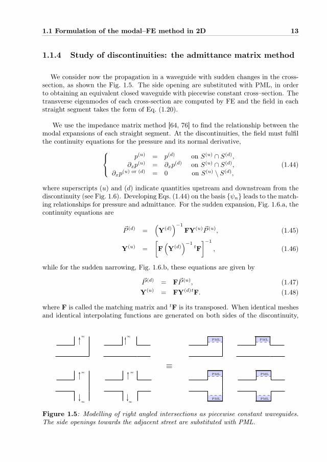
We consider now the propagation in a waveguide with sudden changes in the cross-section, as shown the Fig. 1.5. The side opening are substituted with PML, in orderto obtaining an equivalent closed waveguide with piecewise constant cross–section. Thetransverse eigenmodes of each cross-section are computed by FE and the field in eachstraight segment takes the form of Eq. (1.20).
We use the impedance matrix method [64, 76] to find the relationship between themodal expansions of each straight segment. At the discontinuities, the field must fulfilthe continuity equations for the pressure and its normal derivative,
p(u) = p(d) on S(u) ∩ S(d),∂xp
(u) = ∂xp(d) on S(u) ∩ S(d),
∂xp(u) or (d) = 0 on S(u) \ S(d),
(1.44)
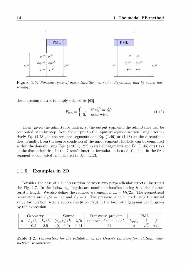
where superscripts (u) and (d) indicate quantities upstream and downstream from thediscontinuity (see Fig. 1.6). Developing Eqs. (1.44) on the basis ψn leads to the match-ing relationships for pressure and admittance. For the sudden expansion, Fig. 1.6.a, thecontinuity equations are
~P (d) =(
Y(d))−1
FY(u) ~P (u), (1.45)
Y(u) =
[
F
(
Y(d))−1
tF
]−1
, (1.46)
while for the sudden narrowing, Fig. 1.6.b, these equations are given by
~P (d) = F~P (u), (1.47)
Y(u) = FY
(d)tF. (1.48)
where F is called the matching matrix and tF is its transposed. When identical meshes
and identical interpolating functions are generated on both sides of the discontinuity,
PML
PML
PML
PML PML
PML
∞
∞
∞
∞
∞∞
≡
Figure 1.5: Modelling of right angled intersections as piecewise constant waveguides.The side openings towards the adjacent street are substituted with PML.
14 1 The modal–FE method
p(d)p(u) p(u) p(d)
Y(u)
Y(d)
Y(u)
Y(d)
PML
a) b)
∂xp(u) ∂xp
(d)
PML
∂xp(u) ∂xp
(d)
S(u) S(u) S(d)S(d)
Figure 1.6: Possible types of discontinuities: a) suden Expansion and b) suden nar-rowing.
the matching matrix is simply defined by [65]
Fmn =
1, if z(d)m = z(u)n
0, otherwise.(1.49)
Then, given the admittance matrix at the output segment, the admittance can becomputed, step by step, from the output to the input waveguide section using alterna-tively Eq. (1.28), in the straight segments and Eq. (1.46) or (1.48) at the discontinu-ities. Finally, from the source condition at the input segment, the field can be computedwithin the domain using Eqs. (1.20)–(1.27) in straight segments and Eq. (1.45) or (1.47)at the discontinuities. In the Green’s function formulation is used, the field in the firstsegment is computed as indicated in Sec. 1.1.3.
1.1.5 Examples in 2D
Consider the case of a L–intersection between two perpendicular streets illustratedthe Fig. 1.7. In the following, lengths are nondimensionalised using h as the charac-teristic length. We also define the reduced wavenumber ka = kh/2π. The geometricalparameters are L1/h = 5/3 and L2 = 1. The pressure is calculated using the initialvalue formulation, with a source condition ~P (0) in the form of a gaussian beam, givenby the expression
Geometry Source Transverse problem PMLh La/h Lb/h (xs, zs)/h λ/h number of elements/λ hPML A β
1 −0.5 2.5 (0,−0.9) 0.21 4− 21 λ√2 π/4
Table 1.2: Parameters for the validation of the Green’s function formulation. Geo-metrical parameters

1.1 Formulation of the modal–FE method in 2D 15
h
L1 L2
x0
YL~P0
z
Figure 1.7: Geometry of the L–intersection.
P0n = e−(zn−zs)2
2σ2 , (1.50)
where zs = −h/2 is the central point and σ = 0.4 the standard deviation, that deter-mines the width of the beam. The rigid wall imposed an output admittance YL = [0].The maximum mesh size mms is fixed to mms = λ/30, which generates 61 nodes inthe first section and 91 nodes in the second section. The inner boundary of the PMLis placed at z = 0, with parameters hPML = λ,A = 2 and β = π/5. The resultingacoustic field is shown in Fig. 1.8a. The result is compared to a full–FE simulationperformed with the Matlab PDE Toolbox (Fig. 1.8b). The mesh size and the PML arethe same in both cases, but in the full-FE computation the PML is placed at z = 1.Since the PML creates an anechoic termination, the result should be independent onthe PML position. Therefore, both results should be identical in the region z < 0. Tocorroborate this, Fig. 1.8d superposes both solutions at z = −0.9. We observe a verygood agreement between with the full-FE simulation.
If desired, it is possible to compute the acoustic field on the side street along thez–direction. For this, we expand the input pressure p(x, z = 0) on the basis of thehorizontal modes φm(x) transverse section of the side street,
φm(x) =
√
2− δm0
L2cos
(mπ
L2(x− L1)
)
, (1.51)
with m ∈ N. The pressure in the side street reads
p(x, z > 0) =
∞∑
m=0
Amφm(x)ekz,mz, (1.52)
with kz,m =√
k2 − (mπ/L2)2 and Am the coefficients of the modal expansion,
Am =
∫ L1+L2
L1
p(x, z = 0)φm(x)dx. (1.53)

16 1 The modal–FE method
The result shown in the Fig. 1.8c is the same as that in Fig. 1.8b, except that the fieldalong the adjacent street has been computed using Eq. (1.52). For this computation,the series (1.52) was truncated to 30 modes, from which 4 modes are propagative. Acomparison with the reference solution at z = 0.5 (dashed arrows in Figs. 1.8b and 1.8c)is shown in Fig. 1.8d. The agreement with the full-FE computation is excellent.
Three extra examples using the Green’s function formulation are shown in theFigs. 1.9a–c. The frequency of the point source is ka = kh/2π = 4.8. The outputcondition is YL = [0] Fig. 1.9a and YL = ΦΓΦ
−1 Fig. 1.9a and Fig. 1.9b. The max-imum mesh size was fixed to mms = λ/21. Notice that the continuity of the pressurefield at the discontinuities is fulfilled perfectly.
p(b)FEM
e)d)
p(b)FEM
p(b)modal−FE
p(a)FEM
p(a)modal−FE
p(a)FEM
p(a)FEM
a) b) c)
p(a)modal−FE
p(b)modal−FE
0.5 1 1.5 2 2.50x/h
0 0.5 1 1.5 2 2.5x/h
0 0.5 1 1.5 2 2.5x/h
0
0.2
0.4
0.6
0.8
1
0 0.5 1 1.5 2 2.5 1.8 2 2.2 2.4 2.6x/h x/h
|p|
|p|
0
0.2
0.4
0.6
0.8
1
0.50.40.30.20.1
0.60.70.80.9
-1
-0.5
0
0.5
1
1.5
-1
-0.5
0
0.5
1
1.5
-1
-0.5
0
0.5
1
1.5
PML
PML
z/h
Figure 1.8: Modulus of the pressure in the L–shaped intersection. a) modal–FE result.b) Full FEM result. c) modal–FE result computing the field in the adjacent street withEq (1.52) d) Pressure fields at z = −0.9. e) Pressure fields at z = 0.5.
x/h
z/hz/h
x/hx/h
a) c)b)
z/h
0 1 2 3 4 5
Rep
-0.15
-0.1
-0.05
0
0.05
0.1
0.15
0.2
0.25
-5
-4
-3
-2
-1
0
1
-4
-3.5
-3
-2.5
-2
-1.5
-1
-0.5
0
0 0.5 1 1.5 2 2.5 3
-2.5
-2
-1.5
-1
-0.5
0
0.5
0 1 2 3 4 5
.
Figure 1.9: Real part of the pressure field in a),b) a T–shaped intersection and c) across intersection. The source position is indicated the symbols "+".
1.2 Extension to 3D geometries 17
b)a) PML
x = L
zx
y
zx
yx = 0
~B
~A
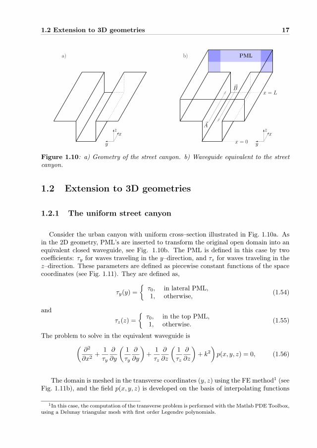
Figure 1.10: a) Geometry of the street canyon. b) Waveguide equivalent to the streetcanyon.
1.2 Extension to 3D geometries
1.2.1 The uniform street canyon
Consider the urban canyon with uniform cross–section illustrated in Fig. 1.10a. Asin the 2D geometry, PML’s are inserted to transform the original open domain into anequivalent closed waveguide, see Fig. 1.10b. The PML is defined in this case by twocoefficients: τy for waves traveling in the y–direction, and τz for waves traveling in thez–direction. These parameters are defined as piecewise constant functions of the spacecoordinates (see Fig. 1.11). They are defined as,
τy(y) =
τ0, in lateral PML,1, otherwise,
(1.54)
and
τz(z) =
τ0, in the top PML,1, otherwise.
(1.55)
The problem to solve in the equivalent waveguide is(∂2
∂x2+
1
τy
∂
∂y
(1
τy
∂
∂y
)
+1
τz
∂
∂z
(1
τz
∂
∂z
)
+ k2)
p(x, y, z) = 0, (1.56)
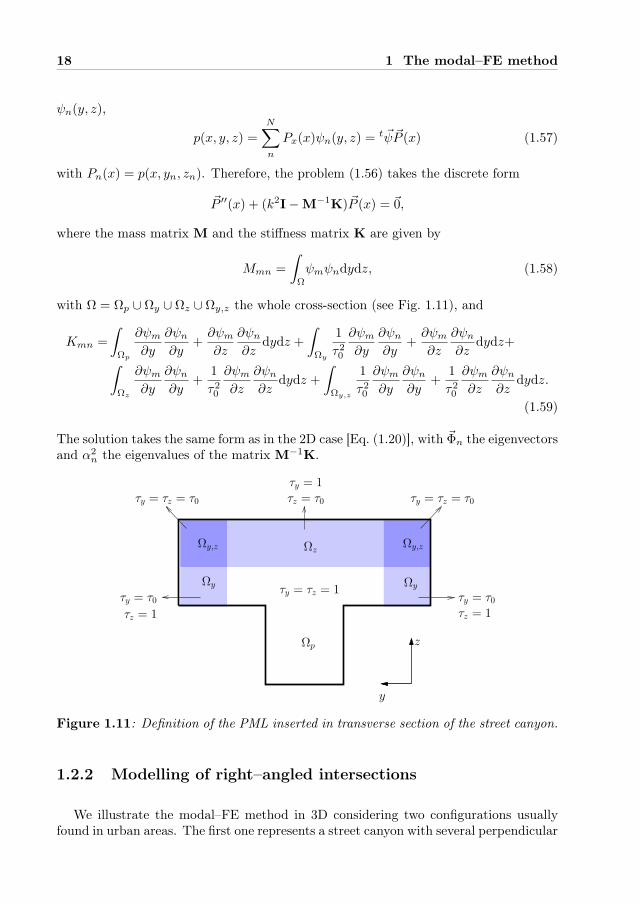
The domain is meshed in the transverse coordinates (y, z) using the FE method1 (seeFig. 1.11b), and the field p(x, y, z) is developed on the basis of interpolating functions
1In this case, the computation of the transverse problem is performed with the Matlab PDE Toolbox,
using a Delunay triangular mesh with first order Legendre polynomials.
18 1 The modal–FE method
ψn(y, z),
p(x, y, z) =
N∑
n
Px(x)ψn(y, z) =t ~ψ ~P (x) (1.57)
with Pn(x) = p(x, yn, zn). Therefore, the problem (1.56) takes the discrete form
~P ′′(x) + (k2I−M−1
K)~P (x) = ~0,
where the mass matrix M and the stiffness matrix K are given by
Mmn =
∫
Ω
ψmψndydz, (1.58)
with Ω = Ωp ∪ Ωy ∪ Ωz ∪ Ωy,z the whole cross-section (see Fig. 1.11), and
Kmn =
∫
Ωp
∂ψm
∂y
∂ψn
∂y+∂ψm
∂z
∂ψn
∂zdydz +
∫
Ωy
1
τ20
∂ψm
∂y
∂ψn
∂y+∂ψm
∂z
∂ψn
∂zdydz+
∫
Ωz
∂ψm
∂y
∂ψn
∂y+
1
τ20
∂ψm
∂z
∂ψn
∂zdydz +
∫
Ωy,z
1
τ20
∂ψm
∂y
∂ψn
∂y+
1
τ20
∂ψm
∂z
∂ψn
∂zdydz.
(1.59)
The solution takes the same form as in the 2D case [Eq. (1.20)], with ~Φn the eigenvectorsand α2
n the eigenvalues of the matrix M−1
K.
Ωy,z Ωy,z
τy = τz = τ0
Ωy Ωy
Ωz
τy = τz = τ0
τy = τ0τz = 1
τy = τ0τz = 1
τy = 1
τz = τ0
τy = τz = 1
Ωp z
y
Figure 1.11: Definition of the PML inserted in transverse section of the street canyon.
1.2.2 Modelling of right–angled intersections
We illustrate the modal–FE method in 3D considering two configurations usuallyfound in urban areas. The first one represents a street canyon with several perpendicular

1.2 Extension to 3D geometries 19
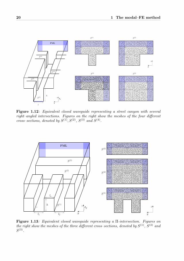
intersecting streets, 1.12. The second one is a Π–intersection, consisting of two parallelstreets intersected by a perpendicular one, 1.13.
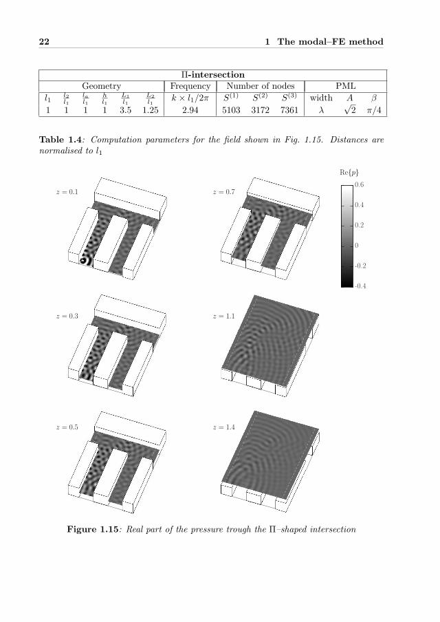
Figs. 1.14 and 1.15 show the real part of the pressure field obtained with the Green’sfunction formulation. The point source position is indicated with symbols "+". Theoutput condition is the characteristic admittance YL = ΦΓΦ
−1. The computationparameters are given in Tabs. 1.3 and 1.4. The figures show horizontal planes of theacoustic field at different heights. Notice the wave guiding within the buildings and theradiation into the atmosphere.
20 1 The modal–FE method
y
zx
y
z
l
h
PML
S(1)
S(2)
S(4)
S(1) S(2)
S(3) S(4)S(3)
Figure 1.12: Equivalent closed waveguide representing a street canyon with severalright–angled intersections. Figures on the right show the meshes of the four differentcross–sections, denoted by S(1), S(2), S(3) and S(4).
PML
y
z
y
zh
la
l2l1
S(1)
S(2)
S(3)
S(1)
S(2)
S(3)
x
Figure 1.13: Equivalent closed waveguide representing a Π-intersection. Figures onthe right show the meshes of the three different cross–sections, denoted by S(1), S(2) andS(3).

1.2 Extension to 3D geometries 21
Right–angled intersectionsGeometry Frequency Meshes PMLl h/l kl/2π S(1) S(2) S(3) S(4) depth A β
1 1.5 1.6 2403 3507 3513 4617 λ√2 π/4
Table 1.3: Computation parameters for the field shown in Fig. 1.14
z = 0.4
z = 0.1
z = 0.7
z = 1
z = 1.3
z = 1.6
Rep
0.4
0.3
0.2
0.1
0
-0.2
-0.1
Figure 1.14: Real part of the pressure in a street with several right angled intersections.
22 1 The modal–FE method
Π-intersectionGeometry Frequency Number of nodes PML
l1l2l1
lal1
hl1
L1
l1L2
l1k × l1/2π S(1) S(2) S(3) width A β
1 1 1 1 3.5 1.25 2.94 5103 3172 7361 λ√2 π/4
Table 1.4: Computation parameters for the field shown in Fig. 1.15. Distances arenormalised to l1
Rep
z = 0.1 z = 0.7
z = 1.4
z = 1.1
z = 0.5
z = 0.3
0
0.2
0.4
0.6
-0.4
-0.2
Figure 1.15: Real part of the pressure trough the Π–shaped intersection

1.3 Summary 23
1.3 Summary
This chapter has introduced the modal–FE method and its application to the mod-eling of different kinds of right–angled intersections. Two formulations have been pro-posed: an initial value formulation, where the source takes the form of a known pressurefield at the input waveguide section; and a Green’s function formulation, enabling us tomodel point sources within the domain. The implementation of the method is dividedin three main steps:
• The original, open geometry is substituted with an equivalent, closed waveguide.
• The transverse eigenmodes of the resulting waveguide are computed with FE andthe general solution in each straight segment is expressed as a function of theseeigenmodes [Eq. (1.20)].
• The modal amplitudes are calculated from the conditions at the waveguide ex-tremities using the impedance matrix method (Sec. 1.1.4).
The modal–FE method can be implemented in any geometry convertible into apiecewise constant waveguide, regardless of the geometry and boundary conditions.Moreover, this approach provides information on the propagation and coupling of thedifferent modes in the medium. This property is very useful in order to gain a fundamen-tal understanding of the studied problems. In addition, since only the transverse sectionis meshed, the computational costs remain low compared to full–numerical methods.We will take advantage of these features to investigate wave propagation phenomena inthe following Chapters.
24 1 The modal–FE method
Appendix 1.A. Perfectly matched layers
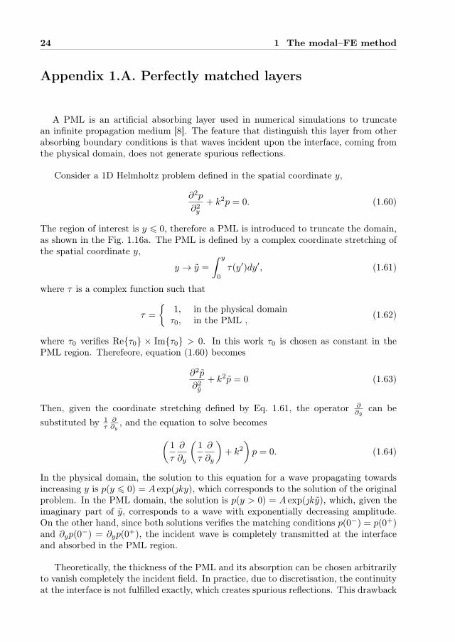
A PML is an artificial absorbing layer used in numerical simulations to truncatean infinite propagation medium [8]. The feature that distinguish this layer from otherabsorbing boundary conditions is that waves incident upon the interface, coming fromthe physical domain, does not generate spurious reflections.
Consider a 1D Helmholtz problem defined in the spatial coordinate y,
∂2p
∂2y+ k2p = 0. (1.60)
The region of interest is y 6 0, therefore a PML is introduced to truncate the domain,as shown in the Fig. 1.16a. The PML is defined by a complex coordinate stretching ofthe spatial coordinate y,
y → y =
∫ y
0
τ(y′)dy′, (1.61)
where τ is a complex function such that
τ =
1, in the physical domainτ0, in the PML ,
(1.62)
where τ0 verifies Reτ0 × Imτ0 > 0. In this work τ0 is chosen as constant in thePML region. Therefeore, equation (1.60) becomes
∂2p
∂2y+ k2p = 0 (1.63)
Then, given the coordinate stretching defined by Eq. 1.61, the operator ∂∂y
can be
substituted by 1τ
∂∂y
, and the equation to solve becomes
(1
τ
∂
∂y
(1
τ
∂
∂y
)
+ k2)
p = 0. (1.64)
In the physical domain, the solution to this equation for a wave propagating towardsincreasing y is p(y 6 0) = A exp(ky), which corresponds to the solution of the originalproblem. In the PML domain, the solution is p(y > 0) = A exp(ky), which, given theimaginary part of y, corresponds to a wave with exponentially decreasing amplitude.On the other hand, since both solutions verifies the matching conditions p(0−) = p(0+)and ∂yp(0
−) = ∂yp(0+), the incident wave is completely transmitted at the interface
and absorbed in the PML region.
Theoretically, the thickness of the PML and its absorption can be chosen arbitrarilyto vanish completely the incident field. In practice, due to discretisation, the continuityat the interface is not fulfilled exactly, which creates spurious reflections. This drawback

1.3 Summary 25
is minimised using a mesh sufficiently fine to describe correctly the exponential decayinside the PML. In this work, we found a satisfactory absorption meshing the PMLwith ten elements and imposing a PML thickness equal to one wavelength.
y
PML
y = 0
a) b)
PML
Reexp(ky)
-1
0
1
y=0
Figure 1.16: a) y–coordinate truncated by a PML at y = 0. b) The field in the PMLis damped exponentially.


Chapter 2
Resonance phenomena in urban
courtyards
Courtyards are frequently found in the city centers of many French and Europeancities (Fig. 2.1 shows some examples). From an acoustical point of view, these enclosedspaces can be regarded as open cavities, which resonances can be excited by wavesgenerated in the urban environment. The goal of this Chapter is to investigate resonancephenomena in these configurations.
This Chapter is based on an articile to be submitted to the Journal of the AcousticalSociety of America [57].
10m 20m20m
c©2012 Google, Tele Atlas c©2012 GeoEye, Google c©2012 AeroWest
Figure 2.1: Typical courtyards considered in this Chapter. Images from left to rightcorrespond to Boteros Street in Seville, Spain; Victor Bonhommet Street in Le Mans,France; and Novalis Street in Berlin, Germany.
27

28 2 Resonance phenomena in urban courtyards
2.1 Introduction
Quiet urban areas are often identified as areas that are not directly exposed to trafficnoise, as the inner yards found in the city centers [61]. However, studies have shownthat inner yards can present considerably high noise levels [40]. This unexpected highlevels of noise are partly generated by interior sources, but also by traffic noise reachingthe courtyard, either above buildings or through façade openings.
Over the last years, authors have studied this problem in several ways. Frequently,the problem is simplified by a two-dimensional (2D) geometry, representing the trans-verse cross-section of two parallel canyons. [38, 40, 60, 83, 84] In such geometry, thesource is placed in one of the canyons and the courtyard is represented by the othercanyon. Authors have investigated in detail the influence of several parameters in noiseshielding, as the roof shape, height-width ratio of the canyon, nature of façade sur-faces [86], noise screens, source type or weather conditions. More recently, Hornikx andForssén [41] investigated the sound propagation in 3D urban courtyards. Apart fromthe parameters mentioned above, this authors evaluated the effect of a façade opening,representing the entrance that connects the courtyard to the adjacent canyon. It wasshown that the noise level inside the courtyard can be increased up to 10 dB(A) inthe frequency band up to 500 Hz with respect to a courtyard without façade openings.Moreover, this work pointed out that a 3D model is necessary to predict correctly thesound level inside the courtyard; differences up to 4.4 dB(A) were found in the noiseabatement estimation with respect to similar 2D configurations.
An additional factor that might increase the sound level inside the courtyard is theexcitation of its acoustic resonances, particularly at low frequency. Such low frequencywaves can be practically measured in urban environments as being produced by eitherheavy industrial machineries, intense impulse noise, or, for a part, the traffic noise[15, 62] and they may propagate on long distances, compared with higher frequencywaves.
This work aims at investigating resonance phenomena in inner yards, both exper-imentally, using a scale model, and numerically, with the modal–FE method. From afundamental point of view, the problem is that of a waveguide (the street) connectedto a side resonator (the courtyard). This setup has been studied extensively in theliterature, due to the intriguing physical phenomena that it exhibits. Fano resonances[35], localized modes [35, 81], negative bulk modulus [25] or nonlinear bandgap behavior[73] have been reported in waveguides connected to side resonators. The present workfocuses on a distinctive characteristic of the 3D urban environment: the wave radiationabove buildings, which enables the interaction between the waveguide and the resonatoreven when no direct connections exists between them. The scope of the present study islimited to the study of two practical aspects regarding urban acoustics applications, theamplification of the sound level inside the courtyard, and the attenuation of the acousticfield transmitted on the street due to the excitation of the courtyard resonances.

2.2 Geometry of the problem 29
Figure 2.2: a) Geometry of the problem. b) Geometrical configurations. Config. A,centered entrance; Config. B, decentered entrance and Config. C, closed entrance.
2.2 Geometry of the problem
Consider a courtyard adjacent to a urban canyon, as shown in Fig. 2.2(a). Thecourtyard is represented by the cavity with dimensions (lc×wc×h). The street canyonhas a rectangular cross–section S = (ws × h) and it is considered as infinitely long inthe x−direction. The courtyard and the street canyon are connected with the entrancedefined by the small volume (le × we × he). The source is placed in the street at thedistance ls from the courtyard in the x–direction. The geometrical parameters are givenin Table. 6.1.
The three geometrical configurations investigated are illustrated in Fig. 2.2(b). Con-figurations A and B correspond to a courtyard with centered entrance and decenteredentrance, respectively. The comparison between Configs. A and B allows us to study theinfluence of the entrance position in the resonance phenomena. Config. C correspondsto a courtyard with closed entrance. The interest of Config. C is twofold. First, thecomparison of Config. C with Configs. A and B allows us to evaluate the impact of thefaçade opening in the resonance phenomena. Secondly, it is relevant to investigate the

30 2 Resonance phenomena in urban courtyards
street canyon courtyard entrance
parameter ls ws h lc wc le we hefull scale (meters) 45 9 12 15 6 3 3 3
1:30 scale model (meters) 1.5 0.3 0.4 0.5 0.2 0.1 0.1 0.1
Table 2.1: Geometrical parameters.
behaviour of this geometry since the only possible interaction with the street is due towaves radiated above the roof level.
2.3 Experimental setup
The experimental setup consists on a 1:30 scale model, as shown in Fig. 2.3.a. Exper-iments are carried out in a semi-anechoic room with walls coated by a melamine foamthat effective from 1 kHz onwards. The ground is made of a plexiglass plate. Buildingsare made of plexiglass blocks with dimensions (0.5× 0.3× 0.4) m. The entrance to thecourtyard is built with 5 cm side varnished wooden cubes. An anechoic terminationmade of melamine dihedrals in inserted at the output to simulate the infinite extensionof the canyon in the x−direction.
The sound source consists on a loudspeaker enclosed in a rigid box, connected tothe canyon by a flanged rectangular duct with cross-section Ss = (5× 5) cm, as shownin Fig. 2.3.b. The transverse field inside the duct should be assumed as constant up to3.4 kHz, the cutoff frequency of the first mode of the cross-section Ss. In this work thefrequency band is limited to 3 kHz, that corresponds to 100 Hz at full scale.
The acoustic pressure is measured using 1/4 in. microphones (B&K 4190), connectedto a preamplifier (B&K 2669) and a conditioning amplifier (B&K Nexus 2669). For themeasurements of insertion losses and transfer functions shown before in Sec. 2.5, themicrophone is placed manually and the acquisition is performed using a SRS analysermodel SR785. For the wave field maps, the microphone position is controlled by a 3Drobotic system. The spatial step is fixed to 20 points per wavelength. The acquisitionof the acoustic pressure is performed using an eInstrument-PC acquisition system fromInnovative Integration. The sampling frequency is fe = 20f (20 samples per period)during a time length Te = Ne/fe, where Ne = 2000 (100 periods) is the number ofsamples. The RMS value of acoustic pressure is estimated by a least mean squaremethod to determine the mean value, the amplitude and the phase of the signal.

2.4 Numerical model 31
b)
buildings
buildings
courtyard
loudspeaker
a)
c)
(3)
(4)
(5)
Ssanechoictermination
(2)(1)
Ss
Figure 2.3: a) Schematics of the experimental setup. b) The acoustic source is aloudspeaker enclosed in a rigid box, which is connected to the canyon through a flangedrectangular duct with cross-section Ss = (5×5) cm. c) (1) Ground made of a plexiglassplate (2) Buildings made of 50cm × 30cm × 40cm plexiglass blocks. (3) Entrance tothe courtyard, built up using 5 cm side wooden cubes. (4) Anechoic termination. (5)Microphones
2.4 Numerical model
The acoustic field in the equivalent waveguide represented in Fig. 2.4a is the solutionto the following problem:
[∂2
∂x2+
1
τ
(∂
∂y
)1
τy
(∂
∂y
)
+1
τz
(∂
∂z
)1
τz
(∂
∂z
)
+ k2]
p = 0, in Ω
∂np = 0, on ∂Ω
(2.1)
where Ω is the domain and ∂Ω its boundaries. The PML parameters τy and τz have beendefined in Sec. 1.2. The problem is meshed in the transverse coordinates y and z andthe eigenmodes of each transverse cross-section are calculated using the FE (Fig. 2.4.b

32 2 Resonance phenomena in urban courtyards
a) b)
Ss
PML
Ω
∂Ω
x
z
y
z
y
Figure 2.4: a) Equivalent waveguide closed with PML. b) Exemples of FEM meshesof the three different cross sections.
shows examples of meshes of the three different cross-sections of the guide). The so-lution in each different straight segment takes general form given in Eq. (1.20). Theoutput condition is defined as a the characteristic admittance, YL = ΦΓΦ
−1, and theadmittance is calculated from the output section to the input the input cross-sectionusing the procedure described in Sec. 1.1.4. Then, we compute the acoustic field in thedomain from an input ~P0 following Eqs. (1.45)–(1.47).
In order to determine the input pressure field that corresponds to the experimentalsource, we define first the input condition as a normal derivative source condition ~U0 =∂x ~P0. From Fig. 2.3.b the components of ~U0 are,
U0,n =
1, if (yn, zn) ∈ Ss
0, elsewhere(2.2)
with (yn, zn) the coordinates of the n−th node. The pressure source condition is theproduct of ~U0 and the input impedance, ~P0 = Y
−10~U0, where is the input Y0.
2.5 Results and discussion 33
2.5 Results and discussion
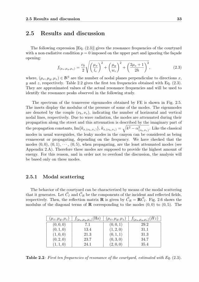
The following expression [Eq. (2.3)] gives the resonance frequencies of the courtyardwith a non-radiative condition p = 0 imposed on the upper part and ignoring the façadeopening:
f(µx,µy,µz) =c02
√(µx
lc
)2
+
(µy
wc
)2
+
(2µz + 1
2h
)2
, (2.3)
where, (µx, µy, µz) ∈ N3 are the number of nodal planes perpendicular to directions x,y and z, respectively. Table 2.2 gives the first ten frequencies obtained with Eq. (2.3).They are approximated values of the actual resonance frequencies and will be used toidentify the resonance peaks observed in the following study.
The spectrum of the transverse eigenmodes obtained by FE is shown in Fig. 2.5.The insets display the modulus of the pressure of some of the modes. The eigenmodesare denoted by the couple (νh, νv), indicating the number of horizontal and verticalnodal lines, respectively. Due to wave radiation, the modes are attenuated during theirpropagation along the street and this attenuation is described by the imaginary part of
the propagation constants, Imkx,(νh,νv), kx,(νh,νv) =√
k2 − α2(νh,νv)
. Like the classical
modes in usual waveguides, the leaky modes in the canyon can be considered as beingevanescent or propagating, depending on the frequency. We have checked that themodes (0, 0), (0, 1), · · · , (0, 5), when propagating, are the least attenuated modes (seeAppendix 2.A). Therefore these modes are supposed to provide the highest amount ofenergy. For this reason, and in order not to overload the discussion, the analysis willbe based only on these modes.
2.5.1 Modal scattering
The behavior of the courtyard can be characterized by means of the modal scatteringthat it generates. Let ~CI and ~CR be the components of the incident and reflected fields,respectively. Then, the reflection matrix R is given by ~CR = R ~CI . Fig. 2.6 shows themodulus of the diagonal terms of R corresponding to the modes (0, 0) to (0, 5). The
(µx, µy, µz) f(µx,µy,µz)(Hz) (µx, µy, µz) f(µx,µy,µz)(Hz)
(0, 0, 0) 7.1 (0, 0, 1) 29.2(0, 1, 0) 13.4 (1, 2, 0) 31.1(1, 0, 0) 21.3 (0, 1, 1) 31.3(0, 2, 0) 23.7 (0, 3, 0) 34.7(1, 1, 0) 24.1 (2, 0, 0) 35.4
Table 2.2: First ten frequencies of resonance of the courtyard, estimated with Eq. (2.3).

34 2 Resonance phenomena in urban courtyards
(0,0)
(0,1)
(0,2)
(1,0)
(1,1)
(1,2)
I
m
α
Reα
(0,0)
(1,0)
(2,0)
(2,1)
(2,2)
(2,3)
(2,4)
(2,5)
(1,1)
(1,3)
(1,4)
(1,5)
(0,5)
(0,3)
(0,4)
(0,1)
(1,2)
(0,2)
-0.16
-0.14
-0.12
-0.1
-0.08
-0.06
-0.04
-0.02
0
0 0.5 1 1.5 2
Figure 2.5: Spectrum of the complex eigenmodes of the transverse waveguide section.The insets display the modulus of some of the corresponding eigenmodes, |~Φ(νy,νz)|.
vertical lines indicate the cutoff frequencies of these modes, given by Ref(νy,νz) (seeFig. 2.6).
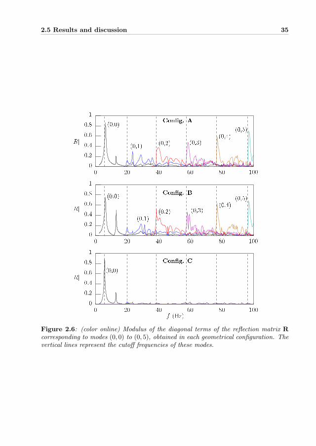
The graphs exhibit several resonance peaks due to the courtyard resonances. Wecorroborate this comparing the position of the peaks with the values in Table 2.2. Thefirst peak at f = 6.3 Hz corresponds to the fundamental resonance of the courtyardf(0,0,0) = 7.1 Hz. The second peak at f = 13 Hz corresponds to the first higherorder resonance f(0,1,0) = 13.4 Hz. Other resonances can also be identified in the band20− 40 Hz as f(0,2,0) = 23.7 Hz, f(0,1,1) = 31.3 Hz and f(0,3,0) = 34.7 Hz. Note that thefrequencies observed in the graphs are slightly lower than those estimated by Eq. (2.3)because of the radiation losses above the courtyard, which are neglected by Eq. (2.3).
The curves of Fig. 2.6 reveal several important characteristics. One is that thecourtyard is very sensitive to the presence of a façade opening. In Configs. A and B(with façade opening) several peaks appear in the reflection coefficients of all modes.The differences between Configs. A and B are explained by the proximity of the entranceto a given nodal plane (this will be discussed in the following sections). In Config. C(without façade opening) the courtyard has a significant effect only for the fundamentalmode (0, 0), and a very weak scattering is observed for higher order modes.
It is also remarkable that the first peak, corresponding to the fundamental resonance,has a similar amplitude in all cases. This indicates that this resonance is mainly excitedby waves propagating above the roof level, being much less sensitive to the presenceof a façade opening. Another important feature is that, given an incident mode, the
2.5 Results and discussion 35
③
Figure 2.6: (color online) Modulus of the diagonal terms of the reflection matrix R
corresponding to modes (0, 0) to (0, 5), obtained in each geometrical configuration. Thevertical lines represent the cutoff frequencies of these modes.

36 2 Resonance phenomena in urban courtyards
Figure 2.7: The insertion loss is computed as Ac = 10 log10 (W0/WT ), where WT
is the energy flux with the courtyard and W0 is the energy flux transmitted through auniform segment of urban canyon with length lc.
modal scattering mainly occurs at resonances close to the cutoff frequency of the mode.Note that the reflection peaks with highest amplitude are comprised between the cutoffof the mode and the cutoff of the next mode. This indicates that the behavior of thecourtyard is strongly linked to the modal content of the incident field.
2.5.2 Insertion Loss
In order to evaluate the attenuation of the acoustic field in the urban canyon due toresonances we calculate the insertion loss, Ac. The energy flux is given by
W =1
2S
∫ ∫
S
Imp∗∂xp dy dz, (2.4)
where “∗” denotes the conjugate. Since the street canyon also induces attenuation dueto radiative losses, the ratio of the incident flux WI to the transmitted flux WT is notenough to determine the attenuation due to the courtyard resonances (see Fig. 2.7).Indeed, the attenuation created by the courtyard alone is computed as
Ac = 10 log10
(WI/WT
WI/W0
)
= 10 log10
(W0
WT
)
, (2.5)
where W0 is the energy flux computed without the courtyard at a distance lc (seeFig. 2.7). Details on the computation of WT and W0 are given in Appendix 2.B.
2.5 Results and discussion 37
♦♥
♦♥
♦♥
③
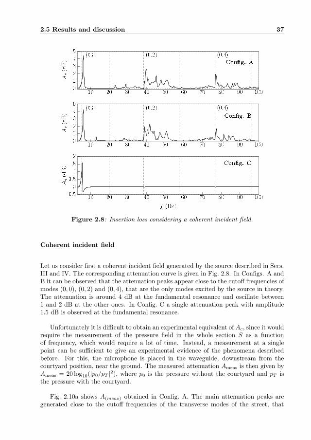
Figure 2.8: Insertion loss considering a coherent incident field.
Coherent incident field
Let us consider first a coherent incident field generated by the source described in Secs.III and IV. The corresponding attenuation curve is given in Fig. 2.8. In Configs. A andB it can be observed that the attenuation peaks appear close to the cutoff frequencies ofmodes (0, 0), (0, 2) and (0, 4), that are the only modes excited by the source in theory.The attenuation is around 4 dB at the fundamental resonance and oscillate between1 and 2 dB at the other ones. In Config. C a single attenuation peak with amplitude1.5 dB is observed at the fundamental resonance.
Unfortunately it is difficult to obtain an experimental equivalent of Ac, since it wouldrequire the measurement of the pressure field in the whole section S as a functionof frequency, which would require a lot of time. Instead, a measurement at a singlepoint can be sufficient to give an experimental evidence of the phenomena describedbefore. For this, the microphone is placed in the waveguide, downstream from thecourtyard position, near the ground. The measured attenuation Ameas is then given byAmeas = 20 log10(|p0/pT |2), where p0 is the pressure without the courtyard and pT isthe pressure with the courtyard.
Fig. 2.10a shows A(meas) obtained in Config. A. The main attenuation peaks aregenerated close to the cutoff frequencies of the transverse modes of the street, that

38 2 Resonance phenomena in urban courtyards
is in good qualitative agreement with the numerical predictions (Fig. 2.8). In orderto visualize the effect of attenuation, the wave field at some relevant frequencies havebeen measured and compared to the numerical fields. The left (resp. right) column ofFig. 2.10b shows horizontal planes of the measured (resp. numerical) fields at f = 6.3 Hzand f = 39.6 Hz, where a strong attenuation of the field is observed. The fields havebeen obtained at height 1.5 m. The mitigation of the acoustic field along the canyon isobvious. At f = 39.6 Hz an attenuation of about 15 dB is found in both the numericaland the experimental fields. At f = 6.3 Hz, the attenuation is about 10 dB in theexperimental field and 15 dB in the numerical field. The cause of this discrepancy isprobably the limited absorption of the room and the anechoic termination at such lowfrequencies (note that the frequency range corresponds to f < 1050 Hz at real scale).
Incoherent incident field
It is also interesting to study the attenuation due to the courtyard in the case of anincident field. Such a field can be found in urban areas as generated by a big numberof uncorrelated sources. If ~PI = Φ ~CI is the incident field, and m and n indicates them−th and n−th node of the mesh in the transverse plane, the definition of an incoherentincident field implies the following condition on ~PI :
< P ∗
I,m, PI,n >= δm,n, (2.6)
where δm,n is the Kronecker symbol, and a unitary amplitude has been assumed (|PI,n| =1). Introducing Eq. (2.6) in the computation of the energy flux (see Appendix A) allowsus to compute the attenuation when a diffuse incident field is considered.
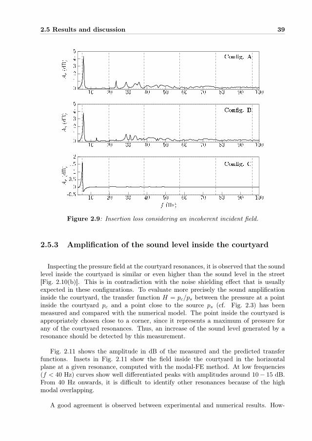
From the point of view of the modes propagating in the street, a diffuse field canbe defined as the superposition of a large number of incoming modes with the sameamplitude and random phase. Then, the attenuation in the incoherent case can beregarded as the averaged attenuation obtained when a large number of realizations isdone, with a single incident mode in each realization. The results in this case shoulddiffer noticeably from the case of the coherent incident field. In particular, the atten-uation is expected to be lower and the concentration of attenuation peaks around thecutoff frequencies should disappear.
The attenuation curves obtained in this case are shown in Fig. 2.9. As expected,the modal behavior observed previously in the coherent case (Fig. 2.8) has disappearedand the attenuation peaks are more uniformly distributed along the frequency range.Also, the absorption peaks have a smaller amplitude. Only the first peak is similar tothat obtained with a coherent source The reason is that at such low frequencies, thesingle propagative mode in the street canyon is the mode (0, 0). Therefore the conceptof incoherent incident field is meaningless. Indeed, whatever the modal content of theincident field at these low frequencies, after a short propagation distance the transversefield in the canyon will be dominated by the mode (0,0). Thus, the attenuation obtainedshould depend weakly on the type of incident field.
2.5 Results and discussion 39
♦♥
♦♥
♦♥
③
Figure 2.9: Insertion loss considering an incoherent incident field.
2.5.3 Amplification of the sound level inside the courtyard
Inspecting the pressure field at the courtyard resonances, it is observed that the soundlevel inside the courtyard is similar or even higher than the sound level in the street[Fig. 2.10(b)]. This is in contradiction with the noise shielding effect that is usuallyexpected in these configurations. To evaluate more precisely the sound amplificationinside the courtyard, the transfer function H = pc/ps between the pressure at a pointinside the courtyard pc and a point close to the source ps (cf. Fig. 2.3) has beenmeasured and compared with the numerical model. The point inside the courtyard isappropriately chosen close to a corner, since it represents a maximum of pressure forany of the courtyard resonances. Thus, an increase of the sound level generated by aresonance should be detected by this measurement.
Fig. 2.11 shows the amplitude in dB of the measured and the predicted transferfunctions. Insets in Fig. 2.11 show the field inside the courtyard in the horizontalplane at a given resonance, computed with the modal-FE method. At low frequencies(f < 40 Hz) curves show well differentiated peaks with amplitudes around 10− 15 dB.From 40 Hz onwards, it is difficult to identify other resonances because of the highmodal overlapping.
A good agreement is observed between experimental and numerical results. How-

40 2 Resonance phenomena in urban courtyards
♦♥
♠s
⑤♣⑤
⑤♣⑤
Figure 2.10: (a) Measured attenuation Ameas obtained in Config. A. (b) Amplitudein dB of the pressure field in the horizontal plane at frequencies f = 6.3 Hz and f =39.6 Hz, obtained in configuration A in source position I. Fields have been measuredat height 5 cm (1.5 m at full scale). Images on the left display measured fields, whileimages on the right display fields calculated with the modal-FE method.

2.5 Results and discussion 41
♦
♦
♦
Figure 2.11: Measured (solid lines) and predicted (dashed lines) amplitude of thetransfer functions in dB. The insets represent the pressure field inside the courtyardat a given resonance.
42 2 Resonance phenomena in urban courtyards
ever, the amplitude of the measured transfer functions are about 5 dB higher than thepredicted ones in the band f < 35 Hz. Again this discrepancy is certainly due to thealready mentioned difficulty of absorbing such low frequencies by the room and the ane-choic termination. Also, it is observed that resonance peaks are more damped in theexperimental case (see, e.g., the first three modes mentioned by the arrows, at ∼ 6.3,13 and 23.6 Hz: the peaks are larger in the experimental results). The reason is thatthe only damping mechanism in the numerical model is the wave radiation above thecourtyard, while in the experimental device other inherent damping phenomena exist,as viscous and thermal losses or a finite impedance of wood.
As it has been observed in the modal reflection coefficients (Fig. 2.6) the positionof the façade opening modifies the behavior of the courtyard. This is explained by theproximity of the entrance to the nodal lines of a given resonance mode (see the insets inFig. 2.11). The most evident example is the peak at f = 23.6 Hz (mode (0, 2, 0)), whichamplitude is more than 5 dB higher in Config. A than in Config. B. The amplitude ofthe second resonance peak at f = 13 Hz is slightly higher in Config. B than in Config. Afor a similar reasons.
Regarding the curve of Config. C, a relevant point is the strong excitation of thefirst two resonant modes. Note that their amplitude is similar to configurations A or Band indicate that the sound level inside the courtyard is only a few decibels lower thanthe source level (0 dB), which is located 45m away. Note also that this confirms theresult predicted previously in Sec. 2.5.1: the excitation of the fundamental resonanceis done mainly by waves propagating above the buildings to reach the courtyard. Withincreasing frequency the resonant behavior is much less pronounced and a decay of thetransfer function is observed. This agrees also with the corresponding curve of Fig. 2.6,that shows a weak excitation of the courtyard resonances from 20 Hz onwards.
2.6 Conclusion
We have investigated numerically and experimentally acoustic resonances in urbancourtyards. Numerical and experimental results are in good agreement and show astrong resonant behaviour of these configurations. As a result of the resonances, thesound level inside the courtyard increases considerably, which generates in turn animportant reduction of the acoustic field on the street. Remarkably, the sound levelinside the courtyard at resonance is comparable to the sound level in the street. On theother hand, the strong interaction between the courtyard resonances and the acousticfield on the street suggests the use of these configurations to control the propagationof low and very low frequency waves in urban environments, which are difficult to becontrolled otherwise.
2.6 Conclusion 43
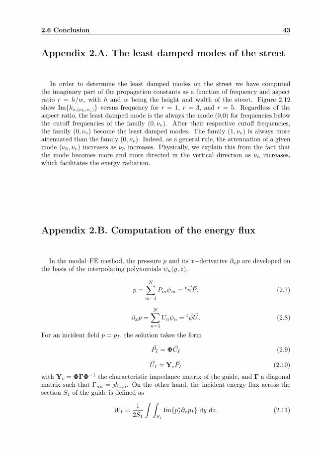
Appendix 2.A. The least damped modes of the street
In order to determine the least damped modes on the street we have computedthe imaginary part of the propagation constants as a function of frequency and aspectratio r = h/w, with h and w being the height and width of the street. Figure 2.12show Imkx,(νh,νv) versus frequency for r = 1, r = 3, and r = 5. Regardless of theaspect ratio, the least damped mode is the always the mode (0,0) for frequencies belowthe cutoff frequencies of the family (0, νv). After their respective cutoff frequencies,the family (0, νv) become the least damped modes. The family (1, νv) is always moreattenuated than the family (0, νv). Indeed, as a general rule, the attenuation of a givenmode (νh, νv) increases as νh increases. Physically, we explain this from the fact thatthe mode becomes more and more directed in the vertical direction as νh increases,which facilitates the energy radiation.
Appendix 2.B. Computation of the energy flux
In the modal–FE method, the pressure p and its x−derivative ∂xp are developed onthe basis of the interpolating polynomials ψn(y, z),
p =
N∑
m=1
Pmψm = t ~ψ ~P , (2.7)
∂xp =N∑
n=1
Unψn = t ~ψ~U. (2.8)
For an incident field p = pI , the solution takes the form
~PI = Φ ~CI (2.9)
~UI = Yc~PI (2.10)
with Yc = ΦΓΦ−1 the characteristic impedance matrix of the guide, and Γ a diagonal
matrix such that Γnn = kx,n. On the other hand, the incident energy flux across thesection S1 of the guide is defined as
WI =1
2S1
∫ ∫
S1
Imp∗I∂xpI dy dz. (2.11)
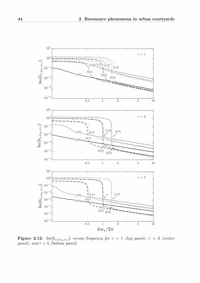
44 2 Resonance phenomena in urban courtyards
(0,0)
(0,0)
(1,0)
(0,0)
(1,0)
(0,1)
(0,1)
(0,1)
(1,3)
(1,3)(1,2)
(0,2)
(0,3)(0,2)
(0,3)
(0,3)(0,2)
(1,0) (1,2)(1,1)(1,3)
(0,1)
(1,1)
10−4
10−3
10−2
10−1
100
101
Imk
xmn
10−5
10−4
10−3
10−2
10−1
100
101
Imk
xmn
10−6
10−5
10−4
10−3
10−2
10−1
100
101
Imk
xmn
r = 1
0.5 1 2 5 10
0.5 1 2 5 10
0.5 1 2 5 10
r = 3
r = 5
kl/2π
Imk
x,(ν
h,νv)
Imk
x,(ν
h,νv)
Imkx,(ν
h,νv)
kws/2π
Figure 2.12: Imkx,(νh,νv) versus frequency for r = 1 (top panel), r = 3 (centerpanel), and r = 5 (bottom panel)

2.6 Conclusion 45
Introducing Eqs. (2.9) and (2.10) into Eq. (2.11) one obtains
WI =1
2S1
N∑
m
N∑
n
Im
P ∗
i,mUi,n
∫ ∫
S1
ψmψndydz
=1
2S1Imt ~P ∗
I GYc~PI
,
(2.12)
where G =∫ ∫
S1ψmψndydz. Similarly, if ~PT = Tn
~PI is the transmitted field, with Tn
the nodal transmission matrix, the transmitted energy flux is given by
WT =1
2S1Imt ~P ∗
ItT
∗
nGYcTn~PI
. (2.13)
The energy flux W0 in the absence of the courtyard has the same form, with Tn thetransmission matrix calculated in the absence of the courtyard (it thus simply describethe damping of the leaky waveguide mode while propagating).
In the case of a diffuse incident field such that < P ∗
I,m, PI,n >= δm,n, one obtainsWT = Im tr (tT∗
nGYcTn), where tr denotes the trace.
The energy flux across the section S of the street is obtained replacing S1 with S inEqs. (2.11)–(2.13) and reducing vectors and matrices to the that nodes located insidethe section S.


Chapter 3
Multimodal approach of the
acoustic propagation in periodic
media
3.1 Introduction
For decades, wave propagation in periodic media has fascinated scientists from differ-ent fields and has motivated intensive research. In the late 80s, Yablanovitch and John[46, 93] proved simultaneously that a transparent material with periodically modulateddielectric properties could avoid the transmission of light at certain frequencies. Suchmaterials were called photonic band gap materials (or photonic crystals), in analogy tothe energy gaps firstly observed in crystalline atomic arrangements [12]. Several yearslater, a similar phenomenon was observed for acoustic waves, giving rise to phononiccrystals (Martínez-Sala et al. [55]). Related to the periodicity, other unique phenomenaare also found in periodic media, as strong dispersion or negative refraction [45, 54].Since their discovery, the interest in phononic crystals has increased enormously, dueto their fundamental interest and also to their application in many areas of science andtechnology (as filtering, wave guiding or superlensing). For an overview of the historicaldevelopment and recent advances on this field, the reader can refer to [75].
In this dissertation, two Chapters are concerned with the wave propagation in peri-odic media: Chapter 4, which investigates the formation of bandgaps in periodic urbanareas; and Chapter 6, which studies the unconventional acoustic response of metasur-faces. Before addressing these challenging studies, the goal of the present Chapter is tointroduce the basic principles of wave propagation in periodic media.
47

48 3 Multimodal approach of the acoustic propagation in periodic media
...
...
...
...
...
...
......
...
...
...
...
...
...
...
...
...
...
...
...
...
...
...
y
x
a) b) c)
Figure 3.1: Geometries under consideration: a) system composed by a single periodicrow along y, b) system composed by a series of periodic rows along y, c) periodic systemalong x and y.
We considered 2D systems composed of periodic arrangements of rectangular scat-terers, Fig. 3.1. Since the modal basis of the transverse sections of these systems canbe obtained analytically, a classical multimodal formulation [64] is used.
3.2 System composed of a single row
Consider the geometry represented by the Fig 3.2. It consists on a single infiniteperiodic row of rectangular rigid scatterers disposed along the y−direction. Lb and hbdenotes respectively the length and the height of the scatterers La is the length of theperiodic free space on both sides of the row, ha is the gap between two consecutivescatterers, and Dy is the period.
When the system is excited with a harmonic plane, the Bloch–Floquet theorem [12]imposes the following condition on the pressure field,
p(x, y + nDy) = enkyDyp(x, y), (3.1)
with n ∈ Z, ky = k sin(θ), and θ the incidence angle with respect to x. This conditionindicates that the acoustic field in the media is also periodic with period Dy, meaningthat the propagation domain can be entirely represented from a single unit cell (Fig. 3.2).
The unit cell is composed of two regions denoted with superscripts (I) and (II). In
the region (I), the pressure field is developed on the basis of plane waves φ(I)n (y) definedby the Bloch–Floquet condition [Eq. (3.1)],
φ(I)n (y) =1
√Dy
eβny, (3.2)

3.2 System composed of a single row 49
...
≡
y
Dy
x
...
La Lb La
θ~A0
(I) (II) (I)
hb2
haDy
Figure 3.2: Left, a system composed by a single periodic row along y. Right, unit cellof the row.
where βn are the Bloch wavenumbers in the y−direction,
βn = ky +2πn
Dy. (3.3)
The pressure field in region (I) takes then form
p(I)(x, y) =
∞∑
n=−∞
φ(I)n (y)(
A(I)n ek
(I)n x +B(I)
n e−k(I)n x)
, (3.4)
with k(I)n =√
k2 − β2n the wavenumbers in the x−direction. In region (II), the pressure
field is developed on the basis of the transverse eigenfunctions (cosine functions in thiscase):
p(II)(x, y) =
∞∑
m=0
(
A(II)m ek
(II)xm
x +Bme−k(II)xm
x)
φ(II)m (y), (3.5)
with
φ(II)m (y) =
√
1 + δm0
hacos
[mπ
ha
(
y − ha2
)]
,
where δ is the Kronecker symbol and k(I)x,m =
√
k2 − (mπ/ha)2.
At the matching sections between the regions, the field must satisfy the continuity

50 3 Multimodal approach of the acoustic propagation in periodic media
conditions for pressure and normal velocity
p(I) = p(II) , |y| ≤ ha/2,
∂xp(I) = ∂xp
(II) , |y| ≤ ha/2.(3.6)
and the rigid boundary condition on the lateral walls
∂xp(I) = 0, |y| > ha/2. (3.7)
The scattering matrix of the single row, Se, relates the incident and scattered waveson each side of the unit cell. This matrix is defined as
(~B0
~AL
)
= Se
(~A0
~BL
)
, (3.8)
where ~A0, ~BL are the modal amplitudes of incident waves, and ~B0, ~AL are the modalamplitudes of reflected waves (see Fig. 3.3a). Since the unit cell is symmetrical withrespect to x, the matrix Se is
Se =
[Re Te
Te Re
]
, (3.9)
with Re and Te the reflection and transmission matrices, valid both for left– andright–going incident waves. These matrices can be calculated using the operator "⋆",defined in Appendix 3.A, which enables us to assemble consecutive scattering elements.Accordingly to Fig. 3.3b, the scattering matrix Se can be expressed as
Se = S1 ⋆ S2 ⋆ S3 ⋆ S4 ⋆ S1, (3.10)
where S1, ...,S4 are the scattering matrices of each of the elements of the cell, consideredseparately. Since elements 1 and 3 are straight segments, its reflection terms are zero
≡
~A0
~B0~AL
~BL
b)a)
S3 S4 S1S1 S2Se
Figure 3.3: a) Incident and scattered waves on each side of the unit cell. Se indi-cates the scattering matrix of the cell. b) Decomposition of the unit cell in elementaryscattering elements. S1 − S4 indicate the scattering matrices of each element.

3.3 System composed of Nr rows 51
matrices [0] and the corresponding scattering matrices S1 and S3 are simply given by
S1 =
[[0] D
(I)(L1)D
(I)(L1) [0]
]
, (3.11)
S3 =
[[0] D
(II)(L2)D
(II)(L2) [0]
]
, (3.12)
with D(i)(x) = diagexp(k(i)xnx), i = I, II. Matrices S2 and S4 are obtained from
the modal expansions of the continuity equations (3.6) and (3.7). From the admittancematrix technique presented in Sec. 1.1.4, these matrices are obtained as
S2 =
[Rb Ta
Tb Ra
]
, (3.13)
S4 =
[Ra Tb
Ta Rb
]
, (3.14)
with,
Ra =
[
I+ F
(
Γ(I))−1 (
tF
∗Γ(II))]−1 [
F
(
Γ(I))−1 (
tF
∗Γ(II))
− I
]
,
Ta =(
Γ(I))−1
tF
∗Γ(II) (I−Ra) ,
Rb =(
Γ(1) + t
F∗Γ(II)
F
)−1 (
Γ(I) − t
F∗Γ(II)
F
)
,
Tb = F (I+Rb) ,
where Γ(i) = diag
k(i)xn
, i = I, II, I is the identity matrix, F is the matching matrix,
defined as,
Fmn =
∫ hb/2
−hb/2
φ(I)n φ(II)m dy, (3.15)
and tF
∗ the conjugate transpose of F.
3.3 System composed of Nr rows
The scattering matrix, Sg, of a system composed of Nr periodic rows can be calculatedsimply from the scattering matrices of each row, Sej , j = 1, 2, . . . , Nr (Fig. 3.4). Thematrix Sg is given by
Sg = Se1 ⋆ Se2 ⋆ ... ⋆ SeNr. (3.16)
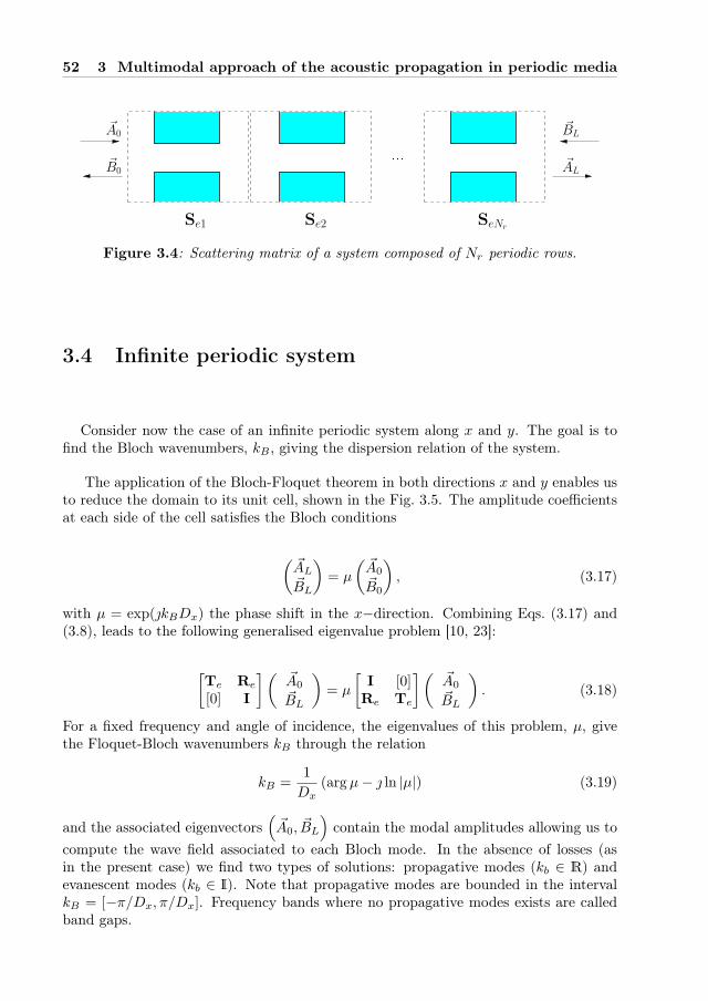
52 3 Multimodal approach of the acoustic propagation in periodic media
...~B0
Se1 Se2 SeNr
~A0~BL
~AL
Figure 3.4: Scattering matrix of a system composed of Nr periodic rows.
3.4 Infinite periodic system
Consider now the case of an infinite periodic system along x and y. The goal is tofind the Bloch wavenumbers, kB , giving the dispersion relation of the system.
The application of the Bloch-Floquet theorem in both directions x and y enables usto reduce the domain to its unit cell, shown in the Fig. 3.5. The amplitude coefficientsat each side of the cell satisfies the Bloch conditions
(~AL
~BL
)
= µ
(~A0
~B0
)
, (3.17)
with µ = exp(kBDx) the phase shift in the x−direction. Combining Eqs. (3.17) and(3.8), leads to the following generalised eigenvalue problem [10, 23]:
[Te Re
[0] I
](~A0
~BL
)
= µ
[I [0]Re Te
](~A0
~BL
)
. (3.18)
For a fixed frequency and angle of incidence, the eigenvalues of this problem, µ, givethe Floquet-Bloch wavenumbers kB through the relation
kB =1
Dx(argµ− ln |µ|) (3.19)
and the associated eigenvectors(
~A0, ~BL
)
contain the modal amplitudes allowing us to
compute the wave field associated to each Bloch mode. In the absence of losses (asin the present case) we find two types of solutions: propagative modes (kb ∈ R) andevanescent modes (kb ∈ I). Note that propagative modes are bounded in the intervalkB = [−π/Dx, π/Dx]. Frequency bands where no propagative modes exists are calledband gaps.
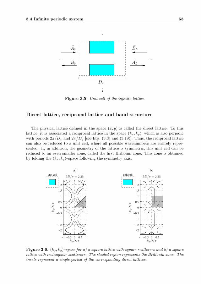
3.4 Infinite periodic system 53
~B0
~BL~A0
~AL
Dx
... ...
...
...
Figure 3.5: Unit cell of the infinite lattice.
Direct lattice, reciprocal lattice and band structure
The physical lattice defined in the space (x, y) is called the direct lattice. To thislattice, it is associated a reciprocal lattice in the space (kx, ky), which is also periodicwith periods 2π/Dx and 2π/Dy [see Eqs. (3.3) and (3.19)]. Thus, the reciprocal latticecan also be reduced to a unit cell, where all possible wavenumbers are entirely repre-sented. If, in addition, the geometry of the lattice is symmetric, this unit cell can bereduced to an even smaller zone, called the first Brillouin zone. This zone is obtainedby folding the (kx, ky)–space following the symmetry axis.
−2
−1.5
−1
−0.5
0
0.5
1
1.5
2
−1 −0.5 0 0.5 1
−2
−1.5
−1
−0.5
0
0.5
1
1.5
2
−1 −0.5 0 0.5 1
unit cell unit cell
a) b)
kyD/π
kD/π = 2.35
kxD/π
kD/π = 2.35
kyD/π
kxD/π
Figure 3.6: (kx, ky)–space for a) a square lattice with square scatterers and b) a squarelattice with rectangular scatterers. The shaded region represents the Brillouin zone. Theinsets represent a single period of the corresponding direct lattices.

54 3 Multimodal approach of the acoustic propagation in periodic media
Fig. 3.6 shows the (kx, ky)–space, at a given frequency, for two types of lattice.The first one, Fig. 3.6a, is a square lattice with square scatterers. Since, the lattice isgeometrical with respect to the x−axis, the y−axis and the axis defined by x = y, theBrillouin zone is represented with a triangle. The second case, shown in Fig. 3.6b, is asquare lattice with rectangular scatterers. Since in this case the axis of symmetry arethe x−axis and y−axis, the Brillouin zone is represented with a square. Note that allthe possible solutions are represented inside the Brillouin zone, and the entire (kx, ky)–space can be constructed by successively unfolding this zone. The band structure of thelattice is obtained from the solutions located on the edge of the Brillouin zone.
3.5 Results
3.5.1 Transmission coefficient of a system composed of Nr rows
Consider a lattice composed of Nr periodic rows (see Fig. 3.4), excited at normalincidence, θ = 0, with Dy = Dx = D, Lb = hb = D/2. The energy trasmissioncoefficient of the lattice, T , is
T =Wt
Wi(3.20)
whereWt andWi are respectively the transmitted and incident energy flux, see Eq. (2.4).
From the orthogonality of functions φ(I)n (y), the energy flux is
Wi =1
2kImt ~A
(I)∗0 Γ(I) ~A
(I)0
, (3.21)
Wt =1
2kImt ~A
(I)∗L Γ(I) ~A
(I)L
. (3.22)
The modal expansions are truncated to 15 plane waves in region (I) and 8 modes inregion (II). Fig. 3.7a shows the transmission coefficient vs. the reduced wavenumberkD/π. The curves shows the variation of T for Nr = 2, 4 and 6 rows. We observe theformation of gaps in the transmission coefficient, which attenuation increases with thenumber of rows.
The results are compared to the band structure of the corresponding infinite lattice(see Fig. 3.7b). The dispersion relation exhibit three bandgaps coinciding with the dipsobserved in the transmission coefficient.
3.5.2 Complete band structure of the infinite periodic lattice
Figure 3.8 shows the complete band structure of the system. The result is compared tothe band structure calculated using a plane wave expansion (PWE) code implemented
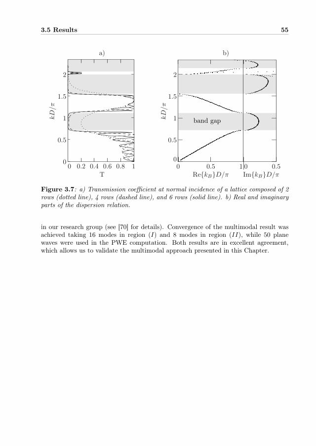
3.5 Results 55
0.5
1
1.5
2
00 0.50.5 1 0
kD/π
b)
RekBD/π ImkBD/π
kD/π
T0.2 0.4 0.6 0.8 10
0.5
1.5
0
1
2
a)
band gap
Figure 3.7: a) Transmission coefficient at normal incidence of a lattice composed of 2rows (dotted line), 4 rows (dashed line), and 6 rows (solid line). b) Real and imaginaryparts of the dispersion relation.
in our research group (see [70] for details). Convergence of the multimodal result wasachieved taking 16 modes in region (I) and 8 modes in region (II), while 50 planewaves were used in the PWE computation. Both results are in excellent agreement,which allows us to validate the multimodal approach presented in this Chapter.

56 3 Multimodal approach of the acoustic propagation in periodic media
1
2
3
4
Γ X
M
kD
/π
Γ ΓX MFigure 3.8: complete band structure of a periodic lattice with dimensions Dy = Dx =D, Lb = hb = D/2. Points represent the multimodal solutions and lines represent thePWE solution.

3.5 Results 57
Appendix 3.A. Assembling of scattering matrices
Consider two scattering objects I and II characterised by their respective scatteringmatrices SI and SII, as indicated in the Fig. 3.9. These matrices are given by
(A2
B1
)
= SI
(A1
B2
)
, (3.23)
SI =
[TI R′
I
RI T ′
I
]
, (3.24)
and (A3
B2
)
= SII
(A2
B3
)
, (3.25)
SII =
[TII R′
II
RII T ′
II
]
. (3.26)
Combining the previous equations, it is possible to find the global scattering matrixSI,II relating the quantities on both extremities [27]:
(A3
B1
)
= SI,II
(A1
B3
)
, (3.27)
SI,II =
[TII(1−R′
IRII)−1TI R′
II + TII(1−R′
IRII)−1R′
IT′
II
RI + T ′
I (1−RIIR′
I)−1RIIR
′
I T ′
I (1−RIIR′
I)−1T ′
II
]
. (3.28)
The previous matrix relation is denoted by de the symbol “⋆”, such that SI,II = SI ⋆SII .
B1 B3B2
A1 A3A2
SI SII
Object IIObject I
Figure 3.9: Assembling of two scattering objects.


Chapter 4
Sound propagation in periodic
urban areas
A regular urban area can be considered, as a first approximation, as a periodic latticeof interconnected streets, see Fig. 4.1 below. Under this assumption specific propertiesof wave propagation in periodic media can be investigated in a urban context. ThisChapter is concerned with the formation of forbidden frequency bands in periodic urbanareas. Particular attention is payed to the effect of radiative losses in the media, anessential characteristic of the urban environment. The Chapter is adapted from of anarticle published in the Journal of Applied Physics [56].
Figure 4.1: Aerial view of The Eixample district, Barcelona (Spain). Image: XavierJubierre / El Periódico
59

60 4 Sound propagation in periodic urban areas
4.1 Introduction
In styling 3D extended distributions of buildings, the assumption of a periodic dis-tribution is convenient to model the acoustic field, as it describes reasonably well somereal situations (see the works by Picaut [69] and Heimann [34]). Doing this, it is possi-ble to investigate the propagation through a large built area, while taking into accountrigorously the three-dimensional characteristics of the problem, as the radiation abovethe streets. Periodic media are known to exhibit peculiar properties (band gaps, strongdispersion, anisotropy, negative refraction) and have attracted a great deal of interestin electromagnetics and optics [45, 54] as, more recently, for acoustic and elastic waves[23, 30, 85, 87, 90, 92]. By assuming a periodic distribution of buildings in modelling thesound propagation in an urban environment, one may thus expect specific properties ofperiodic media to occur. However, would these properties remain in the case (a latticeof open urban Ions) where important radiative losses are generally observed? The aimof this Chapter is to investigate the competitive effects of the periodicity and the waveradiation.
In this work we investigate both experimentally and numerically the specific proper-ties of open periodic lattices, in particular the presence of band gaps. The experimentallattice is made of 9× 26 wooden cuboids, which represent the buildings. The numericalcharacterisation of the lattice is based on the modal–FE formulation of the wave prop-agation within open waveguiding structures, see Chapter 1. It basically consists in afinite element (FE) discretisation of the problem in the transverse section of the waveg-uide (the street) with the open side artificially closed by perfectly matched layers (PML[8]), and a multimodal formulation of the propagation in the longitudinal direction.
The Chapter is organised as follows. Sec. 4.2 shows the experimental device usedin this work. Sec. 4.3 outlines the application of the modal–FE method to the study ofperiodic lattices. Two kinds of problems are treated: an infinite periodic lattice alongone of the horizontal directions and an infinite periodic lattice along the two horizontaldirections. In this section, some common issues on leaky modes and PML modes arediscussed. Experimental and numerical results are presented in Sec. 4.4. The effect ofthe opening is evaluated by comparing the open lattice with an identical one, closedat the top with a rigid boundary. In the sequel, the open lattice is called OL and theclosed one is called CL.
4.2 Experimental setup
The experimental setup is shown in the Fig. 4.2. Experiments are carried out ina semi-anechoic room. Walls are coated with a melamine foam, effective from 1 kHzonwards. The studied lattice is composed of 9×26 rectangular wooden cuboids withspatial periods Dx = Dy = 7.5 cm and obstacles dimensions lx × ly × h = 5 × 5 × 15cm. Thus, the lattice has a total surface of 0.67 × 1.95 m2 and the filling fraction is

4.2 Experimental setup 61
2
11
12
13
14
15
16
25
26
1
source
Mo1
Mo2
Mo3
Mo4
y
Min
Mo5
PC20 KHz AnalyzerB&K ampli.
5cm
7.5cm5cm 7.5cm
15cm
x
yz
x
(III)
(II)
(I)
...
...
1.75m
Figure 4.2: Experimental setup. The image on the left shows a picture of the exper-imental setup. Symbol (I) indicates the parametric antenna, (II) represents a screenpermitting to avoid direct sound transmission over the lattice, (III) indicates the cover-ing used to obtain the CL. The figure on the right shows a schematic representation ofthe experimental setup. The parametric antenna is placed perpendicular to the latticeat the distance 1.75 m. Symbols ’×’ represent microphones positions. The input pres-sure is measured at the position denoted by Min. The output pressure is taken at fivepoints behind the lattice, denoted by Mo1 to Mo5, respectively. Signals are amplified andlowpass filtered to eliminate any remaining high frequency waves radiated by the source.
ff = 44%. A screen is placed above the first row to avoid direct sound propagationfrom the source to the back of the lattice, which could distort the measurements. TheCL is obtained by covering the OL with a wooden board, as indicated by the dashedrectangle in the Fig. 4.2.
f2 − f1 = fsf2
f1f2 + f1
f2 − f1
2f2 2f1
0.1
0.2
0.3
0.4
0.5
0.6
0.7
0.8
0.9
1
0 0.5 1 1.5 2
normalizedpressure amplitude
distance from the source (m)
y(m
)
-0.3
-0.2
0.2
0.3
-0.1
0.1
0
fs
parametricantenna
Figure 4.3: Acoustic field emitted by the parametric antenna in the (x, y)–plane.

62 4 Sound propagation in periodic urban areas
The lattice is excited using a parametric antenna model HSS (HyperSound AudioSystem), product from the American Technology Corporation. From an input signalat frequency fs, the source emits separately two high amplitude ultrasonic waves atfrequencies f1 and f2, related by f2 = f1 + fs, with f1 = 47 kHz. Then, due to non-linear interactions, new spectral components appear, among which are f1−f2, 2f1, f1+f2, 2f2. Because of the increase of attenuation with frequency, the difference frequencycomponent fs = f2−f1 is predominant far from the source, while keeping the ultrasoundproperties. Thus, this device is able to deliver ultra-directive plane waves in the audiblefrequency range.
Fig. 4.3 shows the radiated field, measured at fs = 1.6 kHz. The figure shows highfrequency components in the near field, that vanish approximately 1 m away from thesource. Beyond this distance, only the difference frequency fs remains, and it can beobserved that wavefronts become plane.
Experiments have been performed by placing the antenna at 1.75 m from the latticeand the source signal is a sweep sine from 1 to 8.3 kHz. To fix ideas, this wouldcorrespond to a few tens of a Hertz at "urban" scale. For instance, if the laboratoryexperiment corresponds to 1:100 scale, the frequency range at full scale would be 10 to83 Hz. Such low frequency waves can be practically measured in urban environmentsas being produced by either heavy industrial machineries, intense impulse noise, or, fora part, the traffic noise [16, 63], and they may propagate on long distances, comparedwith higher frequency waves.
The acoustic pressure is measured using 1/2 in. microphones (B&K 4190), con-nected to a preamplifier (B&K 2669) and a conditioning amplifier (B&K Nexus 2669).Additionally, signals are lowpass filtered up to 20 kHz to eliminate any remaining highfrequency component emitted by the source.
With the aim of detecting the band gaps and passbands of the lattice, we measuredthe transfer function between the input and output pressure field. The transfer functionwas obtained as the averaged pressure value at 5 output points, designed by M01 toM05 in Fig. 4.2. The input pressure is measured at the position denoted by Min in thesame figure. A single input point was found to be representative enough of the incidentfield.
We also measured the pressure field on a horizontal plane above the lattice. Thismeasurement was performed using the same system as in Chapter 2
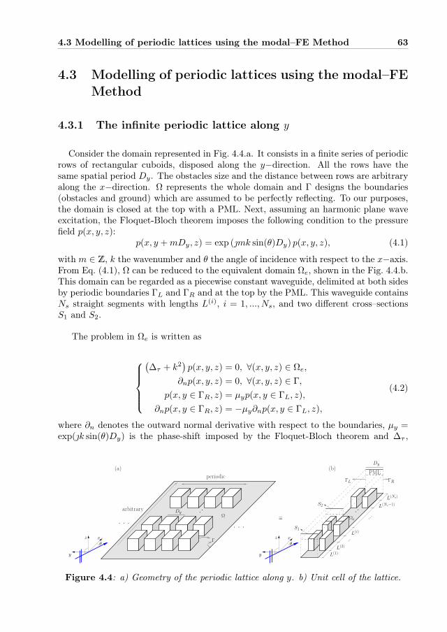
4.3 Modelling of periodic lattices using the modal–FE Method 63
4.3 Modelling of periodic lattices using the modal–FEMethod
4.3.1 The infinite periodic lattice along y
Consider the domain represented in Fig. 4.4.a. It consists in a finite series of periodicrows of rectangular cuboids, disposed along the y−direction. All the rows have thesame spatial period Dy. The obstacles size and the distance between rows are arbitraryalong the x−direction. Ω represents the whole domain and Γ designs the boundaries(obstacles and ground) which are assumed to be perfectly reflecting. To our purposes,the domain is closed at the top with a PML. Next, assuming an harmonic plane waveexcitation, the Floquet-Bloch theorem imposes the following condition to the pressurefield p(x, y, z):
p(x, y +mDy, z) = exp (mk sin(θ)Dy) p(x, y, z), (4.1)
with m ∈ Z, k the wavenumber and θ the angle of incidence with respect to the x−axis.From Eq. (4.1), Ω can be reduced to the equivalent domain Ωe, shown in the Fig. 4.4.b.This domain can be regarded as a piecewise constant waveguide, delimited at both sidesby periodic boundaries ΓL and ΓR and at the top by the PML. This waveguide containsNs straight segments with lengths L(i), i = 1, ..., Ns, and two different cross–sectionsS1 and S2.
The problem in Ωe is written as
(∆τ + k2
)p(x, y, z) = 0, ∀(x, y, z) ∈ Ωe,
∂np(x, y, z) = 0, ∀(x, y, z) ∈ Γ,
p(x, y ∈ ΓR, z) = µyp(x, y ∈ ΓL, z),
∂np(x, y ∈ ΓR, z) = −µy∂np(x, y ∈ ΓL, z),
(4.2)
where ∂n denotes the outward normal derivative with respect to the boundaries, µy =exp(k sin(θ)Dy) is the phase-shift imposed by the Floquet-Bloch theorem and ∆τ ,
θxz
y
θxz
y
Dyarbitrary
periodic
Ω
S1
S2
L(i)
ΓL
Dy
ΓR
PML
Ωe
L(1)
(b)
L(2)
L(Ns−1)
L(Ns)
(a)
. . .. . .
Γ
≡
Figure 4.4: a) Geometry of the periodic lattice along y. b) Unit cell of the lattice.
64 4 Sound propagation in periodic urban areas
defined as
∆τ =∂2
∂x2+
∂2
∂y2+
1
τ
∂
∂z
(1
τ
∂
∂z
)
, (4.3)
denotes the modified Laplacian operator which takes into account the PML. The coef-ficient τ of the PML is given by
τ =
A exp(β), inside the PML,
1, elsewhere,(4.4)
with A > 0 and 0 < β < π/2. The transverse problem is discretised using the FEMand Eqs. (4.2) are transformed into the discrete form
~P ′′(x) +(k2I−M
−1p Kp
)~P (x) = ~0, (4.5)
where Kp,Mp are respectively the stiffness and mass matrices, resulting from the FEMdiscretization of the transverse differential operators, and verifying the lateral Blochconditions (see Appendix 4.A).
In each straight segment, a general solution of (4.5) can be found as a function ofthe eigenvalues α2
n and eigenvectors ~Φn of the matrix M−1p Kp
~P (i)(x) = Φ
(
D(x) ~C1 +D(L(i) − x) ~C2
)
, (4.6)
where Φ = [~Φ1, ~Φ2, ..., ~ΦN ] is the eigenvectors matrix, D(x) is a diagonal matrix suchthat Dnn = exp(kxnx), with kxn = (k2 − α2
n)1/2 the propagation constants, and
vectors ~C1, ~C2 contain the unknowns modal amplitudes for forward and backwardwaves, respectively, which depend on the conditions at the extremities of the segments.To find these coefficients, the mode-matching method is used. The continuity equationsfor pressure and normal velocity are established at the waveguide discontinuities. Then,an output condition is defined by an admittance matrix Y, fulfilling ~U = Y ~P , with ~Uthe x−component of the particle velocity on the basis of the interpolating polynomialsused for the FEM computation. Later, using the continuity equations, the input andoutput admittance matrices of each straight segment are computed, step-by-step, fromthe output to the input segment. Finally, from a source condition, the wave field can beobtained at any point within the domain [27, 28, 64]. The output condition correspondsto the characteristic admittance of the medium.
4.3.2 The infinite periodic lattice along x and y
An infinite periodic lattice along x and y is now considered. A similar process asdescribed in Sec. 3.4 is used to find the Bloch wavenumers kB . The application of the
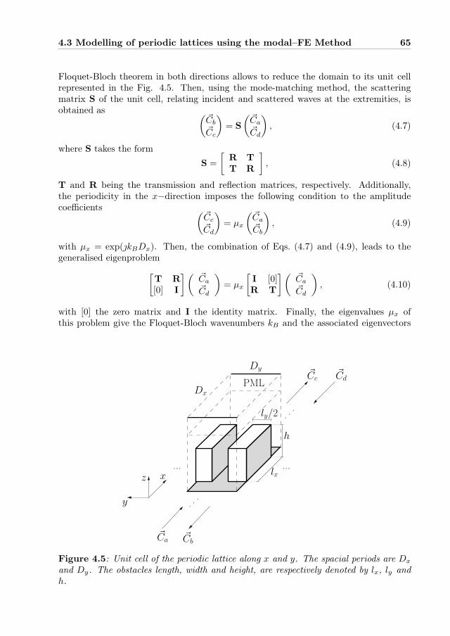
4.3 Modelling of periodic lattices using the modal–FE Method 65
Floquet-Bloch theorem in both directions allows to reduce the domain to its unit cellrepresented in the Fig. 4.5. Then, using the mode-matching method, the scatteringmatrix S of the unit cell, relating incident and scattered waves at the extremities, isobtained as (
~Cb
~Cc
)
= S
(~Ca
~Cd
)
, (4.7)
where S takes the form
S =
[R T
T R
]
, (4.8)
T and R being the transmission and reflection matrices, respectively. Additionally,the periodicity in the x−direction imposes the following condition to the amplitudecoefficients (
~Cc
~Cd
)
= µx
(~Ca
~Cb
)
, (4.9)
with µx = exp(kBDx). Then, the combination of Eqs. (4.7) and (4.9), leads to thegeneralised eigenproblem
[T R
[0] I
](~Ca
~Cd
)
= µx
[I [0]R T
](~Ca
~Cd
)
, (4.10)
with [0] the zero matrix and I the identity matrix. Finally, the eigenvalues µx ofthis problem give the Floquet-Bloch wavenumbers kB and the associated eigenvectors
lx
h
ly/2
~Ca
~Cc ~Cd
~Cb
y
z x... ...
Dy
DxPML
Figure 4.5: Unit cell of the periodic lattice along x and y. The spacial periods are Dx
and Dy. The obstacles length, width and height, are respectively denoted by lx, ly andh.

66 4 Sound propagation in periodic urban areas
(
~Ca, ~Cd
)
contain the amplitude coefficients allowing to compute the wave field for each
mode.
4.3.3 Modelling of closed lattices
Using the techniques described in Secs. 4.3.1 and 4.3.2, the CL is modelled by re-placing the PML termination at the top by a rigid boundary and considering τ = 1 inthe entire domain to obtain the classical Helmholtz equation.
4.3.4 On leaky modes and PML modes
When considering the CL, band gaps and propagative bands are represented by thesolutions µx such that ImkB 6= 0 and ImkB = 0, respectively. In contrast, for theOL, all wavenumbers kB are complex because of the radiation losses above the lattice.Such solutions represent the so-called leaky modes, modes that are partly propagatedthrough the lattice and partly radiated towards the upper part (the Fig. 4.6.b shows anexample). A criterion for discriminate between band gaps and propagative bands forthe leaky modes can be defined by a threshold value η0 of the loss factor
η =
∣∣∣∣
ImkBRekB
∣∣∣∣, (4.11)
from which a given solution can be considered, either propagative η(kB) < η0, orevanescent η(kB) > η0.
Additionally, with the introduction of PML, "PML" modes arises [74, 77]. Thesemodes, strongly localised in the artificial absorbing layer (Fig. 4.6.b), must be discardedsince they do not represent solutions of the original problem. Indeed, they are unphysicalsolutions of the equivalent PML problem. A useful criterion to separate PML modesand leaky modes was proposed by Shi et al. [77], based on the ratio E of the energystored inside the PML volume VPML to the energy stored in the total volume Vtot ofthe unit cell:
E =
∫
VPML|p|2dV
∫
Vtot|p|2dV . (4.12)
From Figs. 4.6.a and 4.6.b, one should expect the ratio E to present values close to zerofor the leaky modes and much higher values for the undesired PML modes.
The main drawback of such criterion is that E must be computed for each solution ofEq. (4.10), which considerably increases the computation time. However, a straightfor-ward way to identify the PML modes comes from the fact that they mainly propagatein the free space above the periodic domain Then, for a given angle of incidence θ,the wavenumbers of PML modes lie close to the so-called sound line, k = kx/ cos(θ),

4.3 Modelling of periodic lattices using the modal–FE Method 67
PMLPML
z(Dx)
z(Dx)
10.80.60.40.20-0.2-0.1
00.1
0.2
0
0.2
0.4
0.6
0.8
x(Dx)y(Dx)
0
0.2
0.4
0.6
0.8
0.40 0.2
0.6 0.8 1
-0.2-0.1
00.1
0.2
x(Dx)y(Dx)
0.5
0.55
0.6
0.65
0.7
0.75
0.8
Leaky modesPML modes
0.6 0.7 0.8 0.9 10.5
kDx/π
k = kx
RekBDx/π
(b)(a)
(c)
Figure 4.6: a) leaky mode, b) PML mode, c) dispersion relation for the leaky (dots)and PML modes (squares) in normal incidence. Note that PML solutions matches thesound line k = kx (dashed line)
representing the dispersion relation of a plane wave propagating in the free space. Thisis illustrated in Fig. 4.6.c, where an arbitrary example of the dispersion relation ofleaky and PML modes with normal incidence (θ = 0) is represented. It is observed thatthe PML solutions match the sound line, while the leaky mode dispersion relation isbended, influenced due to the scattering in the medium. Note that the sound line isanalogous to the light line for electromagnetic waves [77, 80]. This line can be regardedas the transition between evanescent and propagative leaky modes: assuming normalincidence (ky = 0) and considering only the real part of kB , the dispersion relationis approximated by k2 = (RekB)2 + k2z . From this relation, we see that for modesabove the sound line (RekB < k), the vertical wave vector component kz is real. Inother words, these modes are directed vertically, so radiated above the lattice. Modescoinciding with the sound line (RekB = k) represent waves propagating parallel tothe horizontal plane and travelling at the speed of sound in free space. Finally, modesbellow the sound line (RekB > k) become evanescent along z and propagate alongthe x−direction with radiation losses defined by the imaginary part of kB .

68 4 Sound propagation in periodic urban areas
4.4 Results
4.4.1 Band gaps in the lattice
Figs. 4.7.b and 4.8.b show the band structure in normal incidence for the CL andOL, respectively. For the later case, the threshold loss factor η0 is adjusted to η0 = 0.1to filter the evanescent modes, and PML solutions has been eliminated.
In these figures, labels ’mode ν’ denote the number ν of horizontal nodal lines of themode: ’mode 0’ indicates 0 nodal lines; ’mode 1’, 1 nodal line, and so on. Figs. 4.7.cand 4.8.c show the shape of modes 0, 1 and 2 at a given frequency for the CL and theOL, respectively (note that the shape of this modes varies with frequency, although itkeeps the same number of horizontal nodal lines). For the CL, the cutoff frequencies ofthese modes can be obtained by solving the 1D Helmholtz problem along z with rigidboundary conditions. They are given by
f (CL)ν =
νc02h
.
Considering the sound speed c0 = 340 m·s−1, the first three frequencies are f (CL)0,1,2 = 0
Hz, 1133 Hz and 2267 Hz. They are represented by the dashed lines in Fig. 4.7.b.For the OL, the cutoff frequencies of modes 0, 1, 2 are determined by the sound line,represented by the oblique dashed line in Fig. 4.8.b.
Since, with the present configuration, the source impinges uniformly on the inputcross–section of the lattices, one should expect that only the mode 0 will be excited. Forthis reason, the band gaps for this mode have been highlighted, denoted by the shadedregions in Figs. 4.7.b and 4.8.b. Four band gaps are obtained in each case, defined in[1.65− 2.39] kHz, [3.11− 4.18] kHz, [4.72− 5.36] kHz and [6.80− 7.70] kHz for the CLand in [1.70−2.49] kHz, [3.09−4.23] kHz, [4.73−5.39] kHz and [6.80−7.91] kHz for theOL. Note that the band gaps positions for the mode 0 are quite similar in both cases.
Simulated results are compared to the experimental transfer functions shown in theFigs. 4.7.a and 4.8.a. The curves for the OL and CL are quite similar. They alsoshow four band gaps, which are in good agreement with the computed band structures.Nevertheless, some differences in amplitude are visible. For instance, it can be observedthat the first 3 band gaps are more attenuated in the OL, while the fourth band gapis more attenuated in the CL. This could be the result of a weak excitation of higherorder modes, which could vary from one lattice to another. Comparing theoretical andexperimental results, one observes that the measured band gaps are in general wider,surely due to the inherent weak disorder and finite dimensions of the experimentallattice. Other dissipative effects, as the absorption of wood, may also play a role.
Regarding only the first mode, it can be concluded that the main factor governing thebehaviour of this mode is the periodicity in the horizontal directions, while the condition
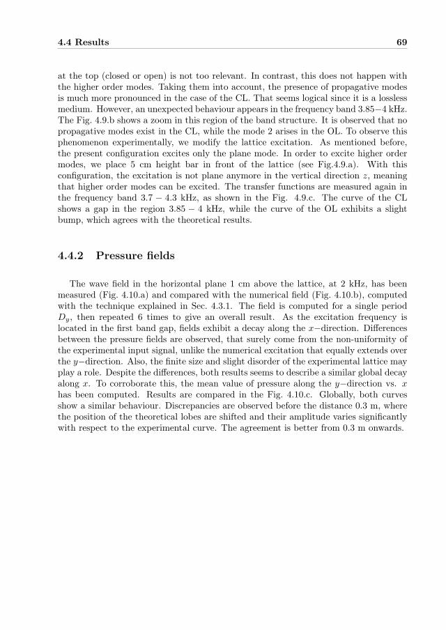
4.4 Results 69
at the top (closed or open) is not too relevant. In contrast, this does not happen withthe higher order modes. Taking them into account, the presence of propagative modesis much more pronounced in the case of the CL. That seems logical since it is a losslessmedium. However, an unexpected behaviour appears in the frequency band 3.85−4 kHz.The Fig. 4.9.b shows a zoom in this region of the band structure. It is observed that nopropagative modes exist in the CL, while the mode 2 arises in the OL. To observe thisphenomenon experimentally, we modify the lattice excitation. As mentioned before,the present configuration excites only the plane mode. In order to excite higher ordermodes, we place 5 cm height bar in front of the lattice (see Fig.4.9.a). With thisconfiguration, the excitation is not plane anymore in the vertical direction z, meaningthat higher order modes can be excited. The transfer functions are measured again inthe frequency band 3.7 − 4.3 kHz, as shown in the Fig. 4.9.c. The curve of the CLshows a gap in the region 3.85 − 4 kHz, while the curve of the OL exhibits a slightbump, which agrees with the theoretical results.
4.4.2 Pressure fields
The wave field in the horizontal plane 1 cm above the lattice, at 2 kHz, has beenmeasured (Fig. 4.10.a) and compared with the numerical field (Fig. 4.10.b), computedwith the technique explained in Sec. 4.3.1. The field is computed for a single periodDy, then repeated 6 times to give an overall result. As the excitation frequency islocated in the first band gap, fields exhibit a decay along the x−direction. Differencesbetween the pressure fields are observed, that surely come from the non-uniformity ofthe experimental input signal, unlike the numerical excitation that equally extends overthe y−direction. Also, the finite size and slight disorder of the experimental lattice mayplay a role. Despite the differences, both results seems to describe a similar global decayalong x. To corroborate this, the mean value of pressure along the y−direction vs. xhas been computed. Results are compared in the Fig. 4.10.c. Globally, both curvesshow a similar behaviour. Discrepancies are observed before the distance 0.3 m, wherethe position of the theoretical lobes are shifted and their amplitude varies significantlywith respect to the experimental curve. The agreement is better from 0.3 m onwards.

70 4 Sound propagation in periodic urban areas
mode 0
mode 0
mode 0
mode 2
mode 1
mode 0
-35 -30 -25 -20 -15 -10 -5 0
Amplitude (dB)
z
yx
c)
f = 1600 Hz f = 3360 Hz f = 3960 Hzmode 0 mode 1 mode 2
1000
2000
3000
4000
5000
6000
7000
8000
0
2000
3000
4000
5000
6000
7000
8000
RekB
Fre
q.
(Hz)
1000
Fre
q.
(Hz)
a) b)
Open lattice
Figure 4.7: Results for the open lattice. a) Measured transfer function. Curves arenormalised to 0 dB for a more comfortable reading. Shaded zones indicates band gaps.b) Band diagrams. Shaded zones indicates band gaps for the mode 0; c) Shape of modes0, 1 and 2 at a given frequency.

4.4 Results 71
mode 1
mode 0
mode 0
mode 0
mode 2
-35 -30 -25 -20 -15 -10 -5 0
mode 0
f = 1600 Hz f = 1130 Hz f = 2300 Hzmode 0 mode 1 mode 2
z
yx
c)
Fre
q.
(Hz)
Fre
q.
(Hz)
1000
2000
3000
4000
5000
6000
7000
8000
Closed lattice
0
1000
2000
3000
4000
5000
6000
7000
8000
RekB
Amplitude (dB)
b)a)
Figure 4.8: Results for the closed lattice. a) Measured transfer function. Curves arenormalised to 0 dB for a more comfortable reading. Shaded zones indicates band gaps.b) Band diagrams. Shaded zones indicates band gaps for the mode 0; c) Shape of modes0, 1 and 2 at a given frequency.

72 4 Sound propagation in periodic urban areas
x
z
mode 2
(c)(b)
4200
4100
4000
3900
3800
3700
4300
open lattice
closed lattice
obstacle
(a)
5cm
open latticeclosed lattice
20150-5-10 5 10RekB
4200
4100
4000
3900
3800
3700
4300
Amplitude (dB)
Figure 4.9: a) position of the obstacle in front of the lattice, used to activate higherorder modes; b) Band structure in the band 3.7 − 4.3 kHz for the CL (dots) and theOL (squares). c) Measured transfer functions for the CL (dotted line) and the OL(continous line). Note that in the band 3.85− 4 kHz no propagative modes exists in theCL, while the mode 2 emerges in the OL.
pre
ssure
amplitu
de
nor
mal
ized
normalized normalized
pressure amplitude pressure amplitude10.90.80.70.60.50.40.30.20.1
0.5
10.9
0.8
0.70.6
0.4
0.30.2
0 0.1 0.2 0.3 0.4 0.5 0.60.1
0.20.3
0.40.5
0.6
0.70.8
0.9
1Experience
Modal-FE
xy
z
(c)
(a) (b)Modal-FEExperience
length of the lattice (m)
Figure 4.10: a) and b) shows respectively the experimental and numerical horizontalplanes of the pressure field at 2 kHz, 1 cm above the lattice. c) averaged pressure in they−direction vs. x for the measured and the numerical fields.
4.5 Conclusion 73
4.5 Conclusion
We have investigated the propagation of acoustic waves in regular urban areas. Theurban area was represented as a periodic lattice of open waveguides. By comparison ofthis open lattice with a more classical, closed lattice, it has been shown that the bandstructure for the first propagating mode remains qualitatively the same when openingthe upper part of the lattice. The measured transfer functions are also very similarin both cases. Thus, for a study involving only the first mode, the problem couldbe simplified to a 2D geometry by eliminating the vertical coordinate. In contrast,significant differences between the closed and the open lattice appear when higher ordermodes are included in the study. As it seems logical, the closed lattice exhibits a moremarked presence of propagative modes. However, results have shown that this behaviourcan be inverted at some frequencies. Unexpectedly, we found propagative bands in theopen lattice that become evanescent in the closed lattice.

74 4 Sound propagation in periodic urban areas
Appendix 4.A. FEM computation of the transverse pe-riodic eigenmodes
The aim of this section is to find the eigenfunctions and eigenvalues of the differentcross–sections S1, ..., S4, shown in Fig. 4.11. For each section, the eigenproblem iswritten as
(∂2
∂y2+
1
τ
∂
∂z
(1
τ
∂
∂z
)
+ α2
)
φ(y, z) = 0, (4.13)
with the set of boundary conditions
∂nφ(y, z) = 0, ∀(y, z) ∈ Γ,
φ(y ∈ ΓR, z) = µyφ(y ∈ ΓL, z),
∂nφ(y ∈ ΓR, z) = −µy∂nφ(y ∈ ΓL, z),
(4.14)
where α,Γ,ΓL and ΓR represent, respectively, the in-plane wavenumber, perfectly re-flecting boundaries, left and right periodic boundaries. For sections S1 or S2, theparameter τ is defined by Eq. (4.4), while for sections S3 or S4, τ = 1 in the entirecross–section. The problem is discretised using linear triangular elements. The meshgenerated satisfies two conditions: firstly, in order to fulfil the periodicity, nodes on ΓR
and ΓL must be symmetrical with respect to the vertical axis of symmetry. Secondly,for simplicity, the modal–FE method requires an identical mesh in the matching sectionS1 ∩ S2 for the OL, or S3 ∩ S4 for the CL [67].
Then, the field φ(y, z) is developed on the basis of the interpolating polynomialsψn(y, z) as
φ(y, z) =
N∑
n=1
Φnψn = t ~ψ~Φ. (4.15)
and the discretised problem takes the form(K− α2
M)~Φ = ~u, (4.16)
where K and M are the stiffness and mass matrix, respectively defined by
Kmn =
∫
Sj
1
τ2
(∂ψm
∂y
∂ψn
∂y+∂ψm
∂z
∂ψn
∂z
)
dydz, (4.17)
and
Mmn =
∫
Sj
ψmψndydz. (4.18)
The vector ~u is the contribution of the normal velocity at boundaries, which terms un

4.5 Conclusion 75
z
y
z
y
closed lattice
S4S3
S2S1
ΓR
Γ
open lattice
ΓL
Figure 4.11: Meshes examples of the transverse cross–sections. Sections S1 and S2
are the cross–section of the open lattice. Sections S3 and S4 are the cross–sections ofthe closed one. Γ are perfectly reflecting boundaries, represented by continuous thicklines. ΓL and ΓR denote the left and right periodic boundaries, represented by dashedlines.
are given by
un =
∫
Γtot
∂nφψndΓtot, (4.19)
with Γtot = Γ ∪ ΓL ∪ ΓR. From (4.19), it is deduced that this terms are equal to zerofor all nodes except for those belonging to the periodic boundaries:
un 6= 0, over ΓL and ΓR
un = 0, elsewhere.
For the section S4, completely bounded by rigid walls, one has ~u = ~0 and the eigenmodesare found as the eigenvalues and eigenvectors of the matrix M
−1K (see Eq. (4.16)).
For the rest, a similar technique as Allard et al. [4] to satisfy the periodic boundaryconditions is used. To turn the notation on a more compact form, the matrix D =K− α2
M is defined and Eq. (4.16) is rewritten as
D~φ = ~u. (4.20)
Following, the problem is arranged so that nodes belonging to ΓL (subscript L) appearfirst, followed by the internal ones (resp. I), and finally by those belonging to ΓR (resp.R). The reordered problem is written as:
DLL DLI DLR
DIL DII DIR
DRL DRI DRR
~ΦL
~ΦI
~ΦR
=
~uL~0~uR
. (4.21)
Also, from Eqs. (4.15) and (4.19), the two last boundary conditions of Eq. (4.14) can

76 4 Sound propagation in periodic urban areas
be traduced by the vectorial expressions
~ΦR = µy
~ΦL
~uR = −µy~uL.(4.22)
Next, introducing Eqs. (4.22) into Eq. (4.21) and eliminating ~ΦR (or ~ΦL) leads to thefollowing eigenproblem for the remaining unknowns ~ΦL (or ~ΦR) and ~ΦI :
Dp
(~ΦL
~ΦI
)
=
(~0~0
)
, (4.23)
with Dp = Kp − α2Mp =
[DLL + µyDLR + µ−1
y DRL +DRR DLI + µ−1y DRI
DIL + µyDIR DII
]
The eigenmodes are given by the eigenvalues α2n and eigenvectors (~ΦL, ~ΦI) of the
matrix M−1p Kp. Note that the eliminated unknowns ~ΦR can be straightforwardly ob-
tained from Eq. (4.22).


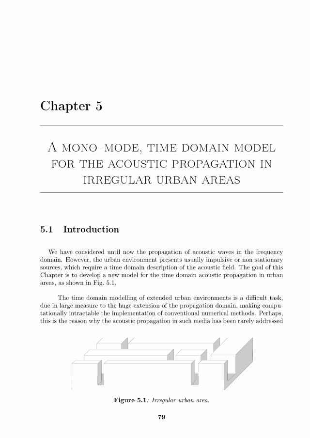
Chapter 5
A mono–mode, time domain model
for the acoustic propagation in
irregular urban areas
5.1 Introduction
We have considered until now the propagation of acoustic waves in the frequencydomain. However, the urban environment presents usually impulsive or non stationarysources, which require a time domain description of the acoustic field. The goal of thisChapter is to develop a new model for the time domain acoustic propagation in urbanareas, as shown in Fig. 5.1.
The time domain modelling of extended urban environments is a difficult task,due in large measure to the huge extension of the propagation domain, making compu-tationally intractable the implementation of conventional numerical methods. Perhaps,this is the reason why the acoustic propagation in such media has been rarely addressed
Figure 5.1: Irregular urban area.
79

805 A mono–mode, time domain model for the acoustic propagation in
irregular urban areas
in the literature. Albert et al. [1, 2] investigated source localisation problems in urbanenvironments using a FDTD approach, although limited to 2D geometries. In a recentwork, Hewett [36] used a ray based model to study the propagation of high frequencywaves in domains containing several interconnected streets. Due to the similarity withthe problem addressed here (a network of interconnected waveguides), one can also men-tion the work by Depollier et al. [21] on a lattice of tubes connected with right–angledjunctions.
The new model proposed in this Chapter is based on a previous characterisation,in the frequency domain, of each of the elements forming the network (waveguides andjunctions). This characterisation is performed using the modal–FE method and theinformation obtained is traduced to the time domain using Fourier analysis. In thetime domain, spatial discretisation is not required and the problem to solve is one–dimensional: the only unknown is the modal amplitude in the waveguide. Therefore,the model is very efficient numerically. Moreover, the model enables us to take intoaccount the complexity of the medium, namely the modal attenuation and dispersion.
5.2 A mono–mode, time domain model
We want to model the acoustic propagation in an irregular urban area as the oneillustrated in Fig. 5.1. The proposed model is based on the following assumptions:
• all the streets have identical cross–section and therefore identical modal basis;
• only the mode (0,0) propagates (see Fig. 2.5)
• the interaction between streets due to wave radiation above the buildings can beneglected
Under these assumption, the urban area can be regarded as a 2D network of inter-connected waveguides in which only one mode propagates. The mode is characterisedby its eigenvector ~Φ(0,0) and its transverse wavenumber α(0,0), which are computed withFE (Sec. 1.2.1).
5.2.1 Propagation in the frequency domain
In each of the waveguides forming the network we define a local longitudinal coordi-nate, χ, as shown in the Fig. 5.2. Taking into account only the mode (0,0), the acousticfield in the frequency domain is given by
~P (χ, f) = ~Φ(0,0)A(χ, f), (5.1)

5.2 A mono–mode, time domain model 81
χ
A(χ, f)
Al(f)
l
A0(f)
L
AL(f)
Figure 5.2: Definition of the local coordinate χ in the waveguide.
where A(χ, f) is the amplitude of the mode as a function χ and frequency f . Thisquantity is expressed as
A(χ, f) = A0(f)ekχχ +AL(f)e
kχ(L−χ), (5.2)
with L the length of the street, kχ =√
k2 − α2(0,0) the propagation constant, A0(f) the
amplitude of the mode at the input section, and AL(f) the amplitude of the mode at theoutput section. For street canyons oriented horizontally, A0 (respectively AL) indicatesthe modal amplitude at the left extremity (respectively, the right extremity). For streetcanyons oriented vertically, A0 (respectively AL) indicates the modal amplitude at thebottom extremity (respectively, the top extremity).
When the mode arrives to a given intersection, its energy is redistributed towardsthe segments connected to the junction. In the frequency domain, this process is de-scribed by the scattering matrix S(f) of the junction junction. We consider two typesof junctions: a T–intersection, characterised by the matrix S⊥(f), and a +–junctioncharacterized by the matrix S+(f) (see Fig. 5.3). These matrices are defined as
Ao,L
Ao,U
Ao,R
= S⊥
Ai,L
Ai,U
Ai,R
, (5.3)
S⊥ =
R⊥1 T⊥3 T⊥1
T⊥2 R⊥2 T⊥2
T⊥1 T⊥3 R⊥1
and
Ao,L
Ao,U
Ao,R
Ao,B
= S+
Ai,L
Ai,U
Ai,R
Ai,B
, (5.4)
S+ =
R+ T+1 T+2 T+1
T+1 R+ T+1 T+2
T+2 T+1 R+ T+1
T+1 T+2 T+1 R+
.

825 A mono–mode, time domain model for the acoustic propagation in
irregular urban areas
a) b)
Ai,L
Ao,L Ai,R
Ao,RAi,L
Ao,L
Ai,UAo,U
Ai,BAo,B
Ai,UAo,U
Ao,R
Ai,R
S⊥ S+
Figure 5.3: a) Definition of the scattering matrix of the T–intersection, S⊥. b) Defi-nition of the scattering matrix of the +–intersection, S+.
In previous equations (5.3) and (5.4), subscripts i and o indicate incident and outgoingwaves, respectively, and subscripts U,B,L and R indicate quantities on the upper,bottom, left and right side from the of the intersection. Note that due to the symmetryof the T–junction the scattering matrix S⊥ has only two different reflection terms R⊥1
and R⊥2, and three transmission terms T⊥1, T⊥2, and T⊥3. Similarly, due to thesymmetry of the +–junction the matrix S+ has only one reflection term R+1 and twotransmission terms T+1 and T+2. Note also that the notation in previous equationscorresponds to the one used in Fig. 5.3. Of course, although the T–junctions mayappear with different orientation, the corresponding scattering matrix would present asimilar form.
The terms of these matrices are calculated using the modal–FE method as explainedin Appendix 5.A. Fig. 5.4 show the modulus and phase of the terms of the scatteringmatrix, corresponding to a street canyon with aspect ratio h/l = 3 (h and l denotes theheight and width of the street). The accident in the curves at kl/2π = 0.07 is due tothe cutoff frequency of the mode, Reα(0,0).
5.2.2 Propagation in the time domain
The inverse Fourier transform (FT−1) of Eq. (5.2) gives the modal amplitude as afunction of time and χ. Given the time convention chosen in this document, exp(−ωt),the FT−1 is defined as
g(t) = FT−1 G(f) =
∫∞
−∞
G(f)e−2πftdf, (5.5)
where G(f) denotes any function of f . Hence, the FT−1 of Eq. (5.2) is
a(χ, t) = a0(t) ∗ d(χ) + aL(t) ∗ d(L− χ), (5.6)
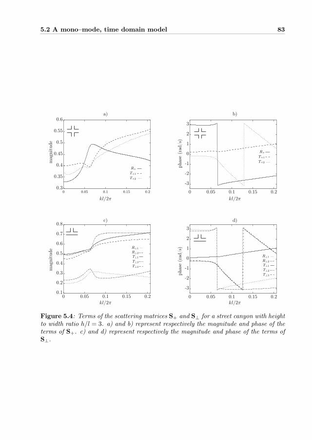
5.2 A mono–mode, time domain model 83
kl/2π kl/2π
c) d)
a) b)
kl/2π kl/2π
mag
nit
ude
mag
nit
ude
phas
e(r
ad/s
)phas
e(r
ad/s
)
0 0.05 0.1 0.15 0.2
R+
T+2
T+1
R+
T+2
T+1
R⊥1
R⊥2
T⊥1
T⊥2
T⊥3
R⊥1
R⊥2
T⊥1
T⊥2
T⊥3
0 0.05 0.1 0.15 0.2
0 0.05 0.1 0.15 0.2 0 0.05 0.1 0.15 0.2
-3
-2
-1
0
1
2
3
-3
-2
-1
0
1
2
3
0.3
0.35
0.4
0.45
0.5
0.6
0.1
0.2
0.3
0.4
0.5
0.6
0.7
0.8
0.55
Figure 5.4: Terms of the scattering matrices S+ and S⊥ for a street canyon with heightto width ratio h/l = 3. a) and b) represent respectively the magnitude and phase of theterms of S+. c) and d) represent respectively the magnitude and phase of the terms ofS⊥.
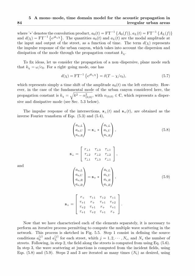
845 A mono–mode, time domain model for the acoustic propagation in
irregular urban areas
where ’∗’ denotes the convolution product, a0(t) = FT−1 A0(f), aL(t) = FT−1 AL(f)and d(χ) = FT−1
ekχχ
. The quantities a0(t) and aL(t) are the modal amplitude at
the input and output of the street, as a function of time. The term d(χ) representsthe impulse response of the urban canyon, which takes into account the dispersion anddissipation of the mode through the propagation constant kχ.
To fix ideas, let us consider the propagation of a non–dispersive, plane mode suchthat kχ = ω/c0. For a right–going mode, one has
d(χ) = FT−1ekχχ
= δ(T − χ/c0), (5.7)
which represents simply a time shift of the amplitude a0(t) on the left extremity. How-ever, in the case of the fundamental mode of the urban canyon considered here, the
propagation constant is kχ =√
k2 − α2(0,0), with α(0,0) ∈ C, which represents a disper-
sive and dissipative mode (see Sec. 5.3 below).
The impulse response of the intersections, s⊥(t) and s+(t), are obtained as theinverse Fourier transform of Eqs. (5.3) and (5.4),
ao,Lao,Uao,R
= s⊥ ∗
ai,Lai,Uai,R
, (5.8)
s⊥ =
r⊥1 τ⊥3 τ⊥1
τ⊥2 r⊥2 τ⊥2
τ⊥1 τ⊥3 r⊥1
,
and
ao,Lao,Uao,Rao,B
= s+ ∗
ai,Lai,Uai,Rai,B
, (5.9)
s+ =
r+ τ+1 τ+2 τ+1
τ+1 r+ τ+1 τ+2
τ+2 τ+1 r+ τ+1
τ+1 τ+2 τ+1 r+
.
Now that we have characterised each of the elements separately, it is necessary toperform an iterative process permitting to compute the multiple wave scattering in thenetwork. This process is sketched in Fig. 5.5. Step 1 consist in defining the sourceconditions a(j)0 and a
(j)L for each street, whith j = 1, 2, · · · , Ns, and Ns the number of
streets. Following, in step 2, the field along the streets is computed from using Eq. (5.6).In step 3, the wave scattering at junctions is computed from the incident fields, usingEqs. (5.8) and (5.9). Steps 2 and 3 are iterated as many times (Nt) as desired, using
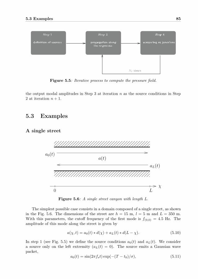
5.3 Examples 85
propagation along
the segments
s attering at jun tionsdenition of sour es
NT times
Step 1 Step 2 Step 3
Figure 5.5: Iterative process to compute the pressure field.
the output modal amplitudes in Step 3 at iteration n as the source conditions in Step2 at iteration n+ 1.
5.3 Examples
A single street
a0(t)
aL(t)
a(t)
χL0
Figure 5.6: A single street canyon with length L.
The simplest possible case consists in a domain composed of a single street, as shownin the Fig. 5.6. The dimensions of the street are h = 15 m, l = 5 m and L = 350 m.With this parameters, the cutoff frequency of the first mode is f(0,0) = 4.5 Hz. Theamplitude of this mode along the street is given by
a(χ, t) = a0(t) ∗ d(χ) + aL(t) ∗ d(L− χ). (5.10)
In step 1 (see Fig. 5.5) we define the source conditions a0(t) and aL(t). We considera source only on the left extremity (aL(t) = 0). The source emits a Gaussian wavepacket,
a0(t) = sin(2πfst) exp(−(T − t0)/σ), (5.11)
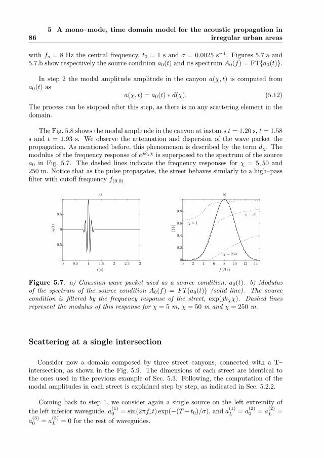
865 A mono–mode, time domain model for the acoustic propagation in
irregular urban areas
with fs = 8 Hz the central frequency, t0 = 1 s and σ = 0.0025 s−1. Figures 5.7.a and5.7.b show respectively the source condition a0(t) and its spectrum A0(f) = FTa0(t).
In step 2 the modal amplitude amplitude in the canyon a(χ, t) is computed froma0(t) as
a(χ, t) = a0(t) ∗ d(χ). (5.12)
The process can be stopped after this step, as there is no any scattering element in thedomain.
The Fig. 5.8 shows the modal amplitude in the canyon at instants t = 1.20 s, t = 1.58s and t = 1.93 s. We observe the attenuation and dispersion of the wave packet thepropagation. As mentioned before, this phenomenon is described by the term dχ. Themodulus of the frequency response of ekχχ is superposed to the spectrum of the sourcea0 in Fig. 5.7. The dashed lines indicate the frequency responses for χ = 5, 50 and250 m. Notice that as the pulse propagates, the street behaves similarly to a high–passfilter with cutoff frequency f(0,0)
t(s) f(Hz)
a) b)
a0(t)
|TF| χ = 1
χ = 250
χ = 50
0 0.5 1 1.5 2 2.5 3 0 2 4 6 8 10 12 14-1
-0.5
0
0.5
1
0
0.2
0.4
0.6
0.8
1
Figure 5.7: a) Gaussian wave packet used as a source condition, a0(t). b) Modulusof the spectrum of the source condition A0(f) = FTa0(t) (solid line). The sourcecondition is filtered by the frequency response of the street, exp(kχχ). Dashed linesrepresent the modulus of this response for χ = 5 m, χ = 50 m and χ = 250 m.
Scattering at a single intersection
Consider now a domain composed by three street canyons, connected with a T–intersection, as shown in the Fig. 5.9. The dimensions of each street are identical tothe ones used in the previous example of Sec. 5.3. Following, the computation of themodal amplitudes in each street is explained step by step, as indicated in Sec. 5.2.2.
Coming back to step 1, we consider again a single source on the left extremity ofthe left inferior waveguide, a(1)0 = sin(2πfst) exp(−(T − t0)/σ), and a(1)L = a
(2)0 = a
(2)L =
a(3)0 = a
(3)L = 0 for the rest of waveguides.

5.3 Examples 87
t = 1.58 s
t = 1.2 s
t = 1.93 s
χ(m)
a(χ, t)
a(χ, t)
a(χ, t)
0 50 100 150 200 250 300 350
0 50 100 150 200 250 300 350
-0.5
-1
0
0.5
1
0 50 100 150 200 250 300 350
-1
-0.5
0
0.5
1
-1
-0.5
0
0.5
1
Figure 5.8: Modal amplitude versus χ at different times.
In step 2, these source conditions are used to compute the modal amplitude alongeach of the canyons. One has
a(1) = a(1)0 ∗ d(χ), (5.13)
a(2) = 0, (5.14)
a(3) = 0. (5.15)
In step 3, the scattering at the intersection is computed from the incident fields usingEq. (5.8). Since in this case the only incident wave is the one arriving from the leftcanyon, the scattered modal amplitudes are given by
ao,Lao,Uao,R
= s⊥ ∗
ai,L00
, (5.16)
where the incident field is in this case ai,L = a(1)0 ∗d(L). Next, output fieldsao,L, ao,U , ao,R
are used as the source conditions a(1)′
0 , a(2)′
L and a(1)′
0 for the next iteration,
a(1)′
0 = ao,L = a(1)0 ∗ d(L) ∗ r⊥1,
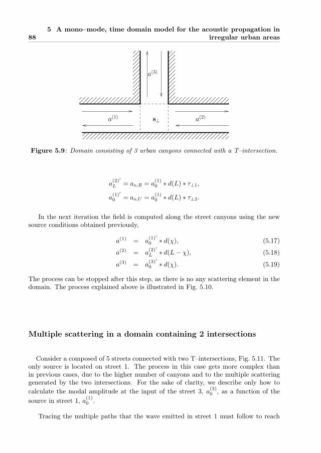
885 A mono–mode, time domain model for the acoustic propagation in
irregular urban areas
s⊥a(1)
a(3)
a(2)
Figure 5.9: Domain consisting of 3 urban canyons connected with a T–intersection.
a(2)′
L = ao,R = a(1)0 ∗ d(L) ∗ τ⊥1,
a(1)′
0 = ao,U = a(1)0 ∗ d(L) ∗ τ⊥2.
In the next iteration the field is computed along the street canyons using the newsource conditions obtained previously,
a(1) = a(1)′
0 ∗ d(χ), (5.17)
a(2) = a(2)′
L ∗ d(L− χ), (5.18)
a(3) = a(3)′
0 ∗ d(χ). (5.19)
The process can be stopped after this step, as there is no any scattering element in thedomain. The process explained above is illustrated in Fig. 5.10.
Multiple scattering in a domain containing 2 intersections
Consider a composed of 5 streets connected with two T–intersections, Fig. 5.11. Theonly source is located on street 1. The process in this case gets more complex thanin previous cases, due to the higher number of canyons and to the multiple scatteringgenerated by the two intersections. For the sake of clarity, we describe only how tocalculate the modal amplitude at the input of the street 3, a(3)0 , as a function of the
source in street 1, a(1)0 .
Tracing the multiple paths that the wave emitted in street 1 must follow to reach

5.3 Examples 89
t = 1.23 s t = 1.85 s
t = 2.5 s t = 3.09 s
Figure 5.10: Wave scattering at the T–intersection.
street 3 (see Fig. 5.11), enables us to write an expression of a(3)0 as
a(3)0 =
term 1︷ ︸︸ ︷
a(1)0 ∗ dL ∗ τ⊥1 ∗ dL ∗ τ⊥1 +
term 2︷ ︸︸ ︷
a(1)0 ∗ dL ∗ τ⊥1 ∗ dL ∗ r⊥1 ∗ dL ∗ r⊥1 ∗ dL ∗ τ⊥1 +
term 3︷ ︸︸ ︷
a(1)0 ∗ dL ∗ τ⊥1 ∗ dL ∗ r⊥1 ∗ dL ∗ r⊥1 ∗ dL ∗ r⊥1 ∗ dL ∗ r⊥1 ∗ dL ∗ τ⊥1 + · · ·
(5.20)
Due to the radiative losses (Imα(0,0)) and the wave radiation towards the sidestreets, the sum (5.20) converges after a finite number of iterations. Recalling that ateach iteration the propagation along a street and the scattering at junctions is computedonce (see Fig. 5.5), we see that the first term of the Eq. (5.20) is obtained after 2iterations, the term 2 is obtained after 4 iterations, the term 3 after 6 iterations, andso on.
In order to evaluate the convergence of Eq. (5.20), Fig. 5.12 shows a30 as a functionof the number of iterations. The influence of the second term is visible after t ≈ 1.5 s,where the curve corresponding to 2 iterations differs from that corresponding to 4iterations. Then, we observe that the results for 4 or 6 iterations are almost identical.This means that the series in Eq. (5.20) can be truncated after the second term, as thesubsequent echoes arriving to street 3 have very weak amplitude.

905 A mono–mode, time domain model for the acoustic propagation in
irregular urban areas
term s
term s
term s
sour e
t
r
r
r
r
t
Figure 5.11: System containing 2 T–intersections. The arrows below indicate the pathsof the multiple reflections arriving to street 3.
2 iterations
4 iterations
6 iterations
t(s)
a(3)
0(t)
0.8 1 1.2 1.4 1.6 1.8 2 2.2 2.4-0.3
-0.2
-0.1
0
0.1
0.2
0.3
Figure 5.12: Transmitted modal amplitude, a(3)0 , as a function of the number of in-
terations: 2 iterations (dotted line), 4 iterations (dashed line), and 6 iterations (solidline).
Urban area
A last example is shown to illustrate the acoustic propagation in the urban areaconsidered initially in Fig 5.1. The dimensions of the transverse sections of the canyonsare l = 10 m and h = 30 m. The length of the streets varies between 40 m, 80 m and120 m. The total extension of the urban area in the horizontal plane is 390× 220 m2.The source is located at the upper left street, and emits a Gaussian wave packet withcentral frequency 6 Hz. Fig. 5.13 shows snapshots of the pressure field at t = 2 s,t = 2.5 s, and t = 3 s. The result was obtained performing 20 iterations.

5.3 Examples 91
t = 2 s
t = 3 s
t = 2.5 s
Figure 5.13: Pressure field in the urban area at t = 2 s, t = 2.5 s, and t = 3 s.
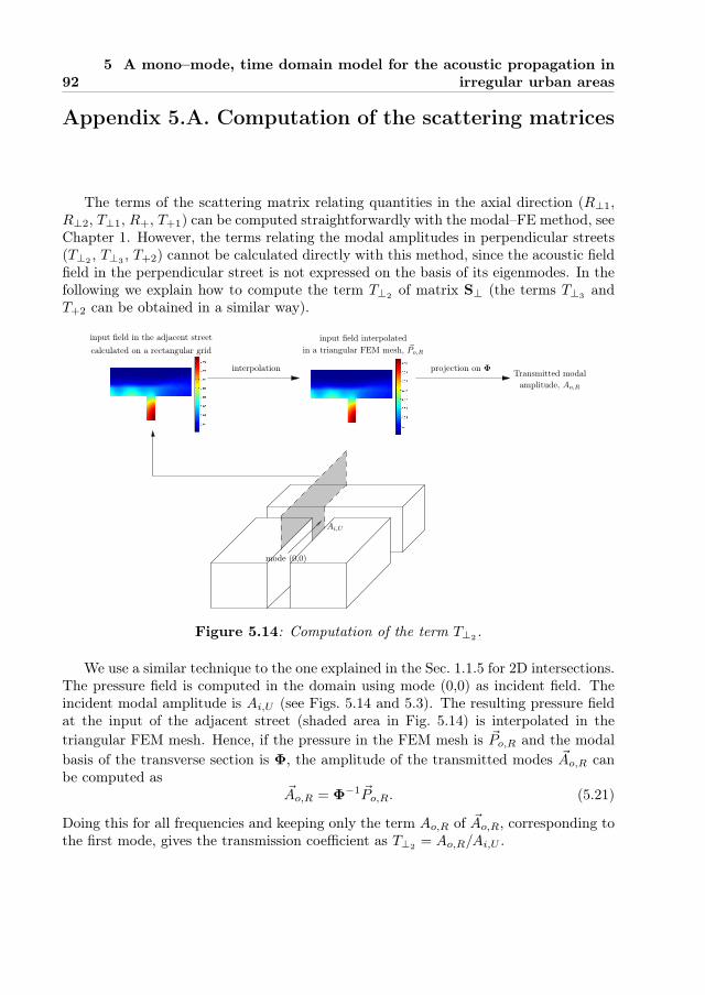
925 A mono–mode, time domain model for the acoustic propagation in
irregular urban areas
Appendix 5.A. Computation of the scattering matrices
The terms of the scattering matrix relating quantities in the axial direction (R⊥1,R⊥2, T⊥1, R+, T+1) can be computed straightforwardly with the modal–FE method, seeChapter 1. However, the terms relating the modal amplitudes in perpendicular streets(T⊥2
, T⊥3, T+2) cannot be calculated directly with this method, since the acoustic field
field in the perpendicular street is not expressed on the basis of its eigenmodes. In thefollowing we explain how to compute the term T⊥2
of matrix S⊥ (the terms T⊥3and
T+2 can be obtained in a similar way).
input field in the adjacent street
Transmitted modalamplitude, Ao,R
calculated on a rectangular grid
input field interpolatedin a triangular FEM mesh, ~Po,R
interpolation
Ai,U
projection on Φ
mode (0,0)
Figure 5.14: Computation of the term T⊥2.
We use a similar technique to the one explained in the Sec. 1.1.5 for 2D intersections.The pressure field is computed in the domain using mode (0,0) as incident field. Theincident modal amplitude is Ai,U (see Figs. 5.14 and 5.3). The resulting pressure fieldat the input of the adjacent street (shaded area in Fig. 5.14) is interpolated in thetriangular FEM mesh. Hence, if the pressure in the FEM mesh is ~Po,R and the modalbasis of the transverse section is Φ, the amplitude of the transmitted modes ~Ao,R canbe computed as
~Ao,R = Φ−1 ~Po,R. (5.21)
Doing this for all frequencies and keeping only the term Ao,R of ~Ao,R, corresponding tothe first mode, gives the transmission coefficient as T⊥2 = Ao,R/Ai,U .


Chapter 6
Controlling the absorption and
reflection of noise barriers using
metasurfaces
6.1 Introduction
The last decade has witnessed an increasing interest in the field of acoustic meta-materials. These materials are defined as artificial structured materials in which thepresence of resonances leads to an unprecedented control on wave propagation [18].The goal of this chapter is to investigate the use of metasurfaces (i.e. two-dimensionalversions of metamaterials) to design noise barriers with advanced acoustic properties.
Most developments on noise barriers have focused on the influence of the head piecein the barrier performance [7, 43, 58], aiming to extend as much as possible the shadowregion behind de barrier; or in developing active control techniques [24]. Here we showthat the use of metasurfaces enables us to obtain some unconventional properties thatcannot be achieved with previous designs.
This study is inspired by recent developments in the field of electromagnetic meta-surfaces [78–80]. These devices are composed of resonant RCL circuits and provide anenhanced control on the directivity of emitting antennas. These properties arises fromthe excitation of resonances in the RCL circuits, which creates a strong dispersion ofthe surface waves propagating on the device. In the present work the RCL circuits arereplaced by C–resonators, Fig. 6.1. As we explain in the following, the presence oflocal resonances in this structure modifies the dispersion characteristics of the acousticsurface waves, giving us the possibility to control de direction of the reflected waves.
95

966 Controlling the absorption and reflection of noise barriers using
metasurfaces
unit
cell
bar
rier
por
ous
laye
r
por
ous
laye
r
PM
L
bar
rier
x3 x2
x1
x3 x2
x1
l
w
h
d
wn
hp
Figure 6.1: Left, metasurface composed of an array of C–resonators. Right, the cor-responding unit cell.
Moreover, it has been demonstrated that an absorbing material backed with an ir-regular surface presents enhanced absorption properties compared to the same materialbacked with a flat surface [26, 29, 31, 32]. In particular, through the excitation ofresonances on the backing surface it is possible to achieve perfect absorption peaks atfrequencies below the quarter–wavelength resonance of the absorbing layer, where thesingle porous material fails [31, 32]. In this Chapter, we demonstrate this behaviourcombining local resonances on the metasurface and an absorbing layer.
6.2 Numerical modeling
The geometry of the problem is illustrated in the Fig. 6.1. It consists on a periodicarrangement of C-resonators disposed over a flat surface. The resonators are coveredwith a porous layer with thickness hp. The spatial period in the horizontal directions isdenoted by D. The geometry of the resonator is defined by its height h, length l, widthw, the neck width wn and the wall thickness d.
6.2.1 Porous material modeling
The porous material is modelled using the 5 parameters Johnson-Champoux-Allardequivalent fluid model [3, 17, 47]. The equivalent speed of sound is defined as ceq =
(ρeqKeq)−1/2 where ρeq and Keq are respectively the dynamic density and compress-
ibility,

6.2 Numerical modeling 97
σ(N · s · m4) ϕ α∞ Λ(m−6) Λ′(m−6)25000 0.98 1.02 90 180
Table 6.1: Parameters of the porous material.
1
Keq=
γP0
ϕ
(
γ − (1− γ)(
1 + ωc
PrωG(Prω)
)−1) , (6.1)
ρeq =ρ0α∞
ϕ
(
1 + ωc
ωF (ω)
)
, (6.2)
with ωc = σϕ/α∞ρ0 the biot frequency, γ the specific heat ratio, P0 the atmosphericpressure, Pr the Prandtl number, ϕ the porosity, α∞ the tortuosity and σ the flowresistivity. The correction functions G(Prω) and F (ω) are given by
G(Prω) =
√
1− ηρ0Prω
(2α∞
σϕΛ′
)2
, (6.3)
F (ω) =
√
1− ηρ0ω
(2α∞
σϕΛ
)2
. (6.4)
In previous Eqs. (6.3) and (6.4), η is the viscosity of the fluid, Λ′ is the thermal char-acteristic length and Λ is the viscous characteristic length. The material employed forthe study is a Fireflex foam, which parameters are given in Tab. 6.1.
6.2.2 Band structure and absorption coeffcient
The modal–FE method is used to model the wave propagation in the unit cell repre-sented in the Fig. 6.1. Considering normal incidence, x3 is the longitudinal coordinateand x1 and x2 are the transverse coordinates. The problem to solve is in this case,
(∂2
∂x21+
∂2
∂x22+
∂2
∂x23+(ω
c
)2)
p(x1, x2, x3) = 0, (6.5)
where c is the sound speed in the unit cell, c = ceq in the porous layer and c = c0elsewhere. Additionally, the field must fulfil rigid boundary conditions at walls, ∂np = 0,and periodic boundary conditions on lateral boundaries, given by
p(x1, x2 +mD,x3) = emkx2Dp(x1, x2, x3), (6.6)
p(x1, x2, x3 + nD) = enkx3Dp(x1, x2, x3). (6.7)

986 Controlling the absorption and reflection of noise barriers using
metasurfaces
For the computation of the surface waves band structure, x1 is the longitudinalcoordinate and x2 and x3 are the transverse coordinates. In this case, we use a PMLaccounting for the wave radiation in the x3 direction. The equation to solve is thengiven by
(∂2
∂x21+
∂2
∂x22+
1
τ
∂
∂x3
(1
τ
∂
∂x3
)
+(ω
c
)2)
p(x1, x2, x3) = 0, (6.8)
where τ is the PML absorbing parameter.
6.3 Control of absorption
The aim of this section is to evaluate the absorption properties of the barrier asa function of the height of the resonators, h. The rest of parameters are fixed toD = 50 cm, w = 40 cm, l = 40 cm, wn = 4 cm, d = 4 cm and hp = 10 cm. An incidentplane wave traveling normal to the surface is considered. The absorption coefficient isdefined as A = 1− R, with R = Wr/Wi the energy reflection coefficient, calculated asthe ratio of the reflected intensity flux Wr to the incident intensity flux Wi.
The top panel in Fig. 6.2 shows the evolution of A forh = 10 cm, h = 20 cm andh = 30 cm. For comparison, two reference solutions are also plotted (bottom graphof Fig. 6.2). One is a porous layer of similar thickness hp backed with a rigid wall.The other one is the same porous layer backed with an air layer of thickness h, andbacked by a rigid wall. We observe an absorption peak that reaches more that 80% atfrequencies well below the quarter wavelength resonance of the porous layer. The peakfrequency is shifted from 500 Hz (h = 10 cm) to 370 Hz (h = 30 cm).
6.4 Control of reflection
Figure 6.3 shows the band structure for waves traveling parallel to the (x1, x2)-planewith an angle θ1 = 50 with respect to the x1-axis. Only the propagative componentsof the Bloch wavenumber are represented, RekB. The sound line, k = kB/ cos(θ1),divides the dispersion relation in two parts. Modes bellow the sound line representacoustic surface waves, which are evanescent in the x3-direction, and are thereforebounded to the surface. Modes above the sound line are propagative along the x3-direction, and are therefore called radiative modes. The former of interest for us, asthey can couple to an incident plane wave impinging the metasurface perpendicularly.
The three curves in Fig. 6.3 correspond to h = 20 cm, h = 25 cm and h = 30 cm.We observe that the dispersion relation of the radiative modes varies with h. In thefollowing we see how the excitation of the radiative modes modifies the waves reflectedon the metasurface.

6.4 Control of reflection 99
A
porous layer only
h = 10cm
h = 30cm
h = 20cm(reference solutions)
A
h = 10 cm
h = 30 cm
h = 20 cm
f (Hz)
f (Hz)
0
0.2
0.4
0.6
0.8
1
0 200 400 600 800 1000
0
1
0.2
0.4
0.6
0.8
0 200 400 600 800 1000
Figure 6.2: Top, absorption coefficient at normal incidence for h = 10 cm, h = 20 cmand h = 30 cm. The inset show the acoustic field at resonance. Bottom, referencesolutions. The dashed line represents the absorption coefficient of the porous layerbacked with a rigid wall. The solid lines corresponds to the porous layer backed with anair layer of thickness h = 10 cm, h = 20 cm and h = 30 cm, and backed with a rigidwall.
The left, central, and right panel in Fig. 6.4 represent the acoustic fields for h =20 cm, h = 25 cm and h = 30 cm, respectively. The impinging wave is a Gaussianbeam with incidence angle θ1 = 50 with respect to x1 and θ2 = 35 with respect toaxis x2. At the excitation frequency, f = 385 Hz, the metasurface presents radiativemodes for h = 20 cm and h = 25 cm (see Fig. 6.3). Hence, we observe the interaction ofthe incident beam with these radiative modes in the corresponding acoustic fields. Aninteresting aspect is that the wave vector of the radiative modes is directed towards thenegative x1 direction [78–80], meaning that the energy which is coupled to these modesis reflected with a negative angle (i.e., in the same direction as the incident beam). Theinterference patterns in the acoustic fields of the left and central panels demonstratethis behaviour. For h = 30 cm (right panel in Fig. 6.4), no radiative modes exist atthe excitation frequency (see dashed line in Fig. 6.3), so that the beam is reflected inthe usual way. This result demonstrates that the excitation of radiative modes on themetasurface can be used to control the wave reflection.
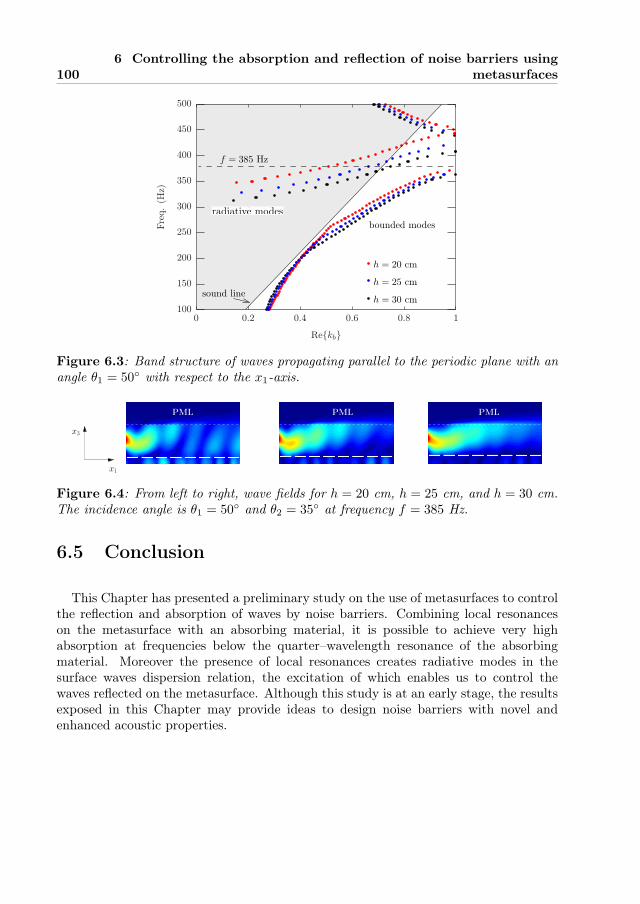
1006 Controlling the absorption and reflection of noise barriers using
metasurfaces
f = 385 Hz
radiated modes
bounded modes
h = 20 cm
h = 25 cm
h = 30 cmsound line
100
150
200
250
300
350
400
450
500
0 0.2 0.4 0.6 0.8 1
Fre
q.
(Hz)
Rekb
radiative modes
Figure 6.3: Band structure of waves propagating parallel to the periodic plane with anangle θ1 = 50 with respect to the x1-axis.
PML PMLPML
x3
x1
Figure 6.4: From left to right, wave fields for h = 20 cm, h = 25 cm, and h = 30 cm.The incidence angle is θ1 = 50 and θ2 = 35 at frequency f = 385 Hz.
6.5 Conclusion
This Chapter has presented a preliminary study on the use of metasurfaces to controlthe reflection and absorption of waves by noise barriers. Combining local resonanceson the metasurface with an absorbing material, it is possible to achieve very highabsorption at frequencies below the quarter–wavelength resonance of the absorbingmaterial. Moreover the presence of local resonances creates radiative modes in thesurface waves dispersion relation, the excitation of which enables us to control thewaves reflected on the metasurface. Although this study is at an early stage, the resultsexposed in this Chapter may provide ideas to design noise barriers with novel andenhanced acoustic properties.


Conclusions and perspectives
We conclude this dissertation with a summary of the main results and ideas for futurework.
In Chapter 1, we have introduced the modal–FE method and its application to themodelling of right–angled intersections. The implementation of the method is dividedin three main steps: (i) the original, open geometry is substituted with an equivalent,closed waveguide; (ii) the transverse eigenmodes of the resulting waveguide are com-puted with FE and introduced in a multimodal description of the acoustic propagationin the longitudinal direction, (iii) The unknown modal amplitudes are calculated usingimpedance matrix method. This method combines the versatility of the FEM, makingit possible to deal with complicated geometries and boundary conditions, and the abil-ity of the multimodal method to provide a good physical understanding of the studiedproblem.
Taking advantage of these features, we have investigated wave phenomena arisingin specific urban urban configurations. In Chapter 2, we have studied the interactionbetween the leaky modes propagating on the street and resonances in an adjacentinner yard. It has been demonstrated that inner yards, supposedly protected from theurban noise, may present significantly high pressure levels due to the excitation of itsacoustic resonances. Moreover, the courtyard resonances attenuates significantly theacoustic field propagating on the street. Remarkably, this phenomenon occurs even inthe absence of a façade opening connecting the courtyard to the street, although onlyat the fundamental courtyard resonance.
After introducing the basic principles of wave propagation in periodic media inChapter 3, we have investigated the acoustic propagation in periodic urban areas inChapter 4. We accomplished this implementing periodic boundary conditions in themodal–FE method and using a scattering matrix approach. The effects of radiativelosses, an essential characteristic of the urban environment, has been studied in detailcomparing the dispersion relation of the open lattice (representing the urban area) tothat of a closed lattice. It was found that the number of propagative modes is in general
103

104 Conclusions and perspectives
smaller in the open lattice, which is attributed to radiative losses. However, we haveseen that there exists evanescent bands in the closed lattice that become propagativebands in the open lattice.
In Chapter 5 we have developed a monomode, time domain model for the acousticpropagation modelling in an irregular urban area, regarded as a network of intercon-nected waveguides. The model is based on a prior characterisation in the frequencydomain of each of the elements forming the network (waveguides and junctions). Thischaracterisation is performed using the modal–FE method and the information obtainedis traduced to the time domain using Fourier analysis. In the time domain, the methoddoes not require spatial discretisation and the problem reduces to obtaining the modalamplitude within the urban canyons. Therefore, the model is very efficient numeri-cally. Despite its relative simplicity and low computational costs, the model takes intoaccount the essential characteristics of the propagation media, as radiative losses andwave dispersion.
The general conclusion coming out from this work is that, despite the presenceof important radiative losses in the propagation media, significant interference andresonance effects are still observed. Not only this result highlights the importance of awave approach to describe accurately low frequency urban acoustic fields, but it suggestthe potential use of these phenomena for controlling the acoustic propagation in urbanenvironments.
The strong interference phenomena reported in this work may motivate the studyof additional wave phenomena in different urban configurations. For instance, it isinteresting to investigate the coupling between multiple resonant courtyards. Also,adding heterogeneities in a regular urban area may induce localised modes of sound[51, 91]. Understanding and exploiting these phenomena may provide ideas to improvethe sound environment at low frequencies.
The time domain model developed in Chapter 5 opens several perspectives for futurework. After incorporating higher order modes to the model, it would be interesting toinvestigate the influence of distinct aspects of the urban morphology in the acousticpropagation, as the building’s shape and size, the effect of disorder or the density ofbuildings. Moreover, the model could be used to extract time indicators in order tocharacterise acoustically the urban area, as the impulse response or the reverberationtime.
Finally, the preliminary results obtained in Chapter 6, together with the rapid devel-opments in the field of acoustic metamaterials and metasurfaces, enables us to foreseethe design of noise barriers with new properties and enhanced performance.


References
[1] Albert, D. G., and Liu, L. The effect of buildings on acoustic pulse propagationin an urban environment. J. Acoust. Soc. Am. 127, 3 (2010), 1335–1346.
[2] Albert, D. G., Liu, L., and Moran, M. L. Time reversal processing for sourcelocation in an urban environment. J. Acoust. Soc. Am. 118, 2 (2005), 616–619.
[3] Allard, J.-F., and Atalla, N. Propagation of sound in porous media. Modellingsound absorbing materials. Wiley,New York, 2009.
[4] Allard, J.-F., Dazel, O., Gautier, G., Groby, J.-P., and Lauriks, W.Prediction of sound reflection by corrugated porous surfaces. J. Acoust. Soc. Am.129, 4 (2011), 1696–1706.
[5] Amir, N., Pagneux, V., and Kergomard, J. A study of wave propagationin varying cross-section waveguides by modal decomposition. Part ii. results. J.Acoust. Soc. Am. 100, 4 (1996), 2034–2048.
[6] Attenborough, K., LI, K., and Horoshenkov, K. Predicting outdoor sound.Taylor & Francis, London and New York, 2006.
[7] Baulac, M., Defrance, J., and Jean, P. Optimization of multiple edge bar-riers with genetic algorithms coupled with a nelder–mead local search. J. SoundVib. 300, 1–2 (2007), 71 – 87.
[8] Berenger, J.-P. A perfectly matched layer for the absorption of electromagneticwaves. J. Comp. Phys. 114, 2 (1994), 185 – 200.
[9] Bot, A. L. A functional equation for the specular reflection of rays. J. Acoust.Soc. Am. 112 (2002), 1276–1287.
[10] Botten, L. C., Nicorovici, N. A., McPhedran, R. C., Sterke, C. M. d.,and Asatryan, A. A. Photonic band structure calculations using scatteringmatrices. Phys. Rev. E 64 (2001), 046603.
107
108 References
[11] Bradley, J. A study of traffic noise around buildings. Acustica 38 (1977), 247–252.
[12] Brillouin, L. Wave propagation in periodic structures, second ed. Dover Publi-cations, Inc., 1953.
[13] Bullen, R., and Fricke, F. Sound propagation in a street. J. Sound Vib. 46(1975), 33 – 42.
[14] Bullen, R., and Fricke, F. Sound propagation at a street intersection in anurban environment. J. Sound Vib. 54, 1 (1977), 123 – 129.
[15] Can, A., Leclercq, L., Lelong, J., and Botteldooren, D. Traffic noisespectrum analysis: Dynamic modeling vs. experimental observations. Appl. Acoust.71 (2010), 764–770.
[16] Can, A., Leclercq, L., Lelong, J., and Botteldooren, D. Traffic noisespectrum analysis: Dynamic modeling vs. experimental observations. Appl. Acoust.71, 8 (2010), 764 – 770.
[17] Champoux, Y., Allard, J., and Lauriks, W. Dynamic tortuosity and bulkmodulus in air saturated porous media. J. Appl. Phys. 70 (1991), 1975–1979.
[18] Craster, R. V., and Guenneau, S. Acoustic metamaterials: negative refrac-tion, imaging, lensing and cloaking. Springer Science & Business Media, 2012.
[19] Davies, H. G. Noise propagation in corridors. J. Acoust. Soc. Am. 53, 5 (1973),1253–1262.
[20] Davies, H. G. Multiple-reflection diffuse-scattering model for noise propagationin streets. J. Acoust. Soc. Am. 64, 2 (1978), 517–521.
[21] Depollier, C., Kergomard, J., and Lesueur, J. Propagation of low frequencyacoustic waves in periodic 2d-lattices of tubes. J. Sound Vib. 142, 1 (1990), 153 –170.
[22] Doc, J.-B., Lihoreau, B., and Félix, S. Higher order padé approximation forthe parabolic equation in a varying cross-section waveguide. Acta Acustica unitedwith Acustica 98 (2012), 691–699.
[23] Duclos, A., Lafarge, D., and Pagneux, V. Transmission of acoustic wavesthrough 2D phononic crystal: visco-thermal and multiple scattering effects. Eur.Phys. J.: Appl. Phys. 45, 1 (2009), 1.
[24] Duhamel, D., Sergent, P., Hua, C., and Cintra, D. Measurement of activecontrol efficiency around noise barriers. Appl. Acoust. 55, 3 (1998), 217 – 241.
[25] Fang, N., Xi, D., Xu, J., Ambati, M., Srituravanich, W., Sun, C., andZhang, X. Ultrasonic metamaterials with negative modulus. Nature Materials 6(2006), 452–456.

References 109
[26] Félix, S., Asch, M., Filoche, M., and Sapoval, B. Localization and increaseddamping in irregular acoustic cavities. J. Sound Vib. 299 (2007), 965–976.
[27] Félix, S., and Pagneux, V. Multimodal analysis of acoustic propagation inthree-dimensional bends. Wave Motion 36, 2 (2002), 157 – 168.
[28] Félix, S., and Pagneux, V. Sound attenuation in lined bends. J. Acoust. Soc.Am. 116, 4 (2004), 1921–1931.
[29] Félix, S., Sapoval, B., Filoche, M., and Asch, M. Enhanced wave absorp-tion through irregular interfaces. Eurpophysics Letters 85 (2009), 14004.
[30] Feng, L., Liu, X.-P., Lu, M.-H., Chen, Y.-B., Chen, Y.-F., Mao, Y.-F.,Zi, J., Zhu, Y.-Y., Zhu, S.-N., and Ming, N.-B. Refraction control of acousticwaves in a square-rod-constructed tunable sonic crystal. Phys. Rev. B 73 (2006),193101.
[31] Groby, J.-P., Duclos, A., Dazel, O., Boeckx, L., and Lauriks, W. Ab-sorption of a rigid frame porous layer with periodic circular inclusions backed bya periodic grating. J. Acoust. Soc. Am. 129, 5 (2011), 3035–3046.
[32] Groby, J.-P., Lauriks, W., and Vigran, T. Total absorption peak by use ofa rigid frame porous layer backed by a rigid multi-irregularities grating. J. Acoust.Soc. Am. 127, 5 (2010), 2865–2874.
[33] Guillaume, G., Picaut, J., Dutilleux, G., and Gauvreau, B. Time-domainimpedance formulation for transmission line matrix modelling of outdoor soundpropagation. J. Sound Vib. 330, 26 (2011), 6467 – 6481.
[34] Heimann, D. Three-dimensional linearised euler model simulations of sound prop-agation in idealised urban situations with wind effects. Appl. Acoust. 68, 2 (2007),217 – 237.
[35] Hein, S., Koch, W., and Nannen, L. Trapped modes and Fano resonancesin two-dimensional acoustical duct-cavity systems. J. Fluid Mech. 692 (2012),257–287.
[36] Hewett, D. P. Sound Propagation in an Urban Environment. PhD thesis, StCatherine’s College. University of Oxford, 2010.
[37] Hornikx, M., and Forssén, J. The 2.5-dimensional equivalent sources methodfor directly exposed and shielded urban canyons. J. Acoust. Soc. Am. 122, 5 (2007),2532–2541.
[38] Hornikx, M., and Forssén, J. A scale model study of parallel urban canyons.Acta Acustica united with Acustica 94 (2008), 265–281.
[39] Hornikx, M., and Forssén, J. Noise abatement schemes for shielded canyons.Appl. Acoust. 70, 2 (2009), 267 – 283.
[40] Hornikx, M., and Forssén, J. Noise abatement schemes for shielded canyons.Appl. Acoust. 70 (2009), 267–283.

110 References
[41] Hornikx, M., and Forssén, J. Modelling of sound propagation to three-dimensional urban courtyards using the extended Fourier PSTD method. Appl.Acoust. 72 (2011), 665–676.
[42] Hu, J., and Menyuk, C. R. Understanding leaky modes: slab waveguide revis-ited. Adv. Opt. Photon 1 (2009), 58–106.
[43] Ishizuka, T., and Fujiwara, K. Performance of noise barriers with various edgeshapes and acoustical conditions. Appl. Acoust. 65, 2 (2004), 125 – 141.
[44] Iu, K. K., and Li, K. M. The propagation of sound in narrow street canyons. J.Acoust. Soc. Am. 112, 2 (2002), 537–550.
[45] Joannopoulos, J. D., Johnson, S. G., Winn, J. N., and Meade, R. D.Photonic Crystals. Molding the flow of light. Princeton University Press, NewJersey, 2008.
[46] John, S. Strong localization of photons in certain disordered dielectric superlat-tices. Phys. Rev. Lett. 58 (1987), 2486–2489.
[47] Johnson, D., Koplik, J., and Dashen, R. Theory of dynamic permeability andtortousity in fluid-saturated porous media. J. Fluid Mech. 176 (1987), 1379–402.
[48] Kang, J. Numerical modelling of the sound fields in urban streets with diffuselyreflecting boundaries. J. Sound Vib. 258 (2002), 793–813.
[49] Kang, J. Numerical modelling of the sound fields in urban square. J. Acoust. Soc.Am. 117 (2005), 3695–3706.
[50] Kang, J. Urban Sound Environment. Taylor & Francis, London and New York,2007.
[51] Khelif, A., Wilm, M., Laude, V., Ballandras, S., and Djafari-Rouhani,B. Guided elastic waves along a rod defect of a two-dimensional phononic crystal.Phys. Rev. E 69 (Jun 2004), 067601.
[52] Lihoreau, B., Gauvreau, B., Bérengier, M., Blanc-Benon, P., and Cal-met, I. Outdoor sound propagation modeling in realistic environments: Appli-cation of coupled parabolic and atmospheric models. J. Acoust. Soc. Am. 120, 1(2006), 110–119.
[53] Lyon, R. H. Role of multiple reflections and reverberation in urban noise propa-gation. J. Acoust. Soc. Am. 55, 3 (1974), 493–503.
[54] Markos, P., and Soukoulis., C. M. Wave Propagation: From Electrons toPhotonic Crystals and Left-Handed Materials. Princeton University Press, NewYersey, 2008.
[55] Matínez-Sala, R., Sancho, J., Sánchez, J. V., Gomez, V., LLinares, J.,and Meseguer, F. Sound attenuation by sculpture. Nature 378 (1995), 241.

References 111
[56] Molerón, M., Félix, S., Pagneux, V., and Richoux, O. Sound propagationin periodic urban areas. J. Appl. Phys. 111, 11 (2012), 114906.
[57] Molerón, M., Félix, S., Pagneux, V., and Richoux, O. Low frequencyacoustic resonances in urban courtyards. J. Acoust. Soc. Am. (to be submitted).
[58] Möser, M., and Volz, R. Improvement of sound barriers using headpieces withfinite acoustic impedance. J. Acoust. Soc. Am. 106, 6 (1999), 3049–3060.
[59] Ögren, M., and Kropp, W. Road traffic noise propagation between two di-mensional city canyons using an equivalent sources approach. Acta Acustica unitedwith Acustica 90(2) (2004), 293–300.
[60] Ögren, M., and W., K. Road traffic noise propagation between two dimen-sional city canyons using an equivalent source approach. Acta Acustica united withAcustica 90 (2004), 293–300.
[61] Öhrström, E., Skåberg, A., and Gidölf-Gunnarsson, A. Effects of roadtraffic noise and the benefit of access to quietness. J. Sound Vib. 295 (2006), 40–59.
[62] Ouis, D. Annoyance from road traffic noise: A review. J. Environ. Psychol. 21(2001), 101–120.
[63] Ouis, D. Annoyance from road traffic noise: a review. J. Environ. Psychol. 21, 1(2001), 101 – 120.
[64] Pagneux, V., Amir, N., and Kergomard, J. A study of wave propagationin varying cross-section waveguides by modal decomposition. Part i. theory andvalidation. J. Acoust. Soc. Am. 100, 4 (1996), 2034–2048.
[65] Pelat, A. Approche modale de la propagation acoustique dans les guides d’ondesouverts. Application à l’acoustique urbaine. PhD thesis, Université du Maine, 2009.
[66] Pelat, A., Félix, S., and Pagneux, V. On the use of leaky modes in openwaveguides for the sound propagation modeling in street canyons. J. Acoust. Soc.Am. 126, 6 (2009), 2864–2872.
[67] Pelat, A., Félix, S., and Pagneux, V. A coupled modal-finite element methodfor the wave propagation modeling in irregular open waveguides. J. Acoust. Soc.Am. 129, 3 (2011), 1240–1249.
[68] Picaut, J. Numerical modeling of urban sound fields by a diffusion process. Appl.Acoust. 63, 9 (2002), 965 – 991.
[69] Picaut, J., Hardy, J., and Simon, L. Sound propagation in urban areas: Aperiodic disposition of buildings. Phys. Rev. E 60 (1999), 4851–4859.
[70] Pichard, H., Richoux, O., and Groby, J.-P. Experimental demonstrationsin audible frequency range of band gap tunability and negative refraction in two-dimensional sonic crystal. J. Acoust. Soc. Am. 132, 4 (2012), 2816–2822.

112 References
[71] Renterghem, T. V., and Botteldooren, D. The importance of roof shapefor road traffic noise shielding in the urban environment. J. Sound Vib. 329, 9(2010), 1422 – 1434.
[72] Renterghem, T. V., Salomons, E., and Botteldooren, D. Parameter studyof sound propagation between city canyons with a coupled FDTD-PE model. Appl.Acoust. 67, 6 (2006), 487 – 510.
[73] Richoux, O., Tournat, V., and Le Van Suu, T. Acoustic wave dispersion ina one-dimensional lattice of non linear resonant scatterers. Phys. Rev. E 75 (2007),026615.
[74] Rogier, H., and De Zutter, D. Berenger and leaky modes in microstrip sub-strates terminated by a perfectly matched layer. IEEE Trans. Microwave TheoryTech. 49, 4 (2001), 712 –715.
[75] Romero-Garcia, V. On the control of propagating acoustic waves in sonic crys-tals: analytical, numerical and optimization techniques. PhD thesis, UniversidadPolitécnica de Valencia, 2010.
[76] Roure, A. Propagation Guidée, étude des discontinuitées. PhD thesis, Universitéd’Aix Marseille, 1976.
[77] Shi, S., Chen, C., and Prather, D. W. Plane-wave expansion method forcalculating band structure of photonic crystal slabs with perfectly matched layers.J. Opt. Soc. Am. A 21 (2004), 1769–1775.
[78] Sievenpiper, D. Forward and backward leaky wave radiation with large effectiveaperture from an electronically tunable textured surface. IEEE Trans. AntennasPropag. 53, 1 (2005), 236–247.
[79] Sievenpiper, D., Schaffner, J., Lee, J., and Livingston, S. A steerableleaky-wave antenna using a tunable impedance ground plane. IEEE AntennasWireless Propag. Lett. 1, 1 (2002), 179 –182.
[80] Sievenpiper, D., Zhang, L., Broas, R., Alexopolous, N., andYablonovitch, E. High-impedance electromagnetic surfaces with a forbiddenfrequency band. IEEE Trans. Microwave Theory Tech. 47, 11 (1999), 2059 –2074.
[81] Sugimoto, N., and Imahori, H. Localized mode of sound in a waveguide withHelmholtz resonators. J. Fluid Mech. 546 (2006), 89–111.
[82] Van Renterghem, T., and Botteldooren, D. Prediction-step staggered-in-time FDTD: an efficient numerical scheme to solve the linearised equations of fluiddynamics in outdoor sound propagation. Appl. Acoust. 68 (2007), 201–216.
[83] Van Renterghem, T., and Botteldooren, D. The importance of roof shapefor road traffic noise shielding in the urban environment. J. Sound Vib. 329 (2010),1422–1434.
References 113
[84] Van Renterghem, T., Salomons, E., and Botteldooren, D. Parameterstudy of sound propagation between city canyons with a coupled FDTD-PE model.Appl. Acoust. 67 (2006), 487–510.
[85] Vasseur, J. O., Deymier, P. A., Khelif, A., Lambin, P., Djafari-Rouhani,B., Akjouj, A., Dobrzynski, L., Fettouhi, N., and Zemmouri, J. Phononiccrystal with low filling fraction and absolute acoustic band gap in the audiblefrequency range: A theoretical and experimental study. Phys. Rev. E 65 (2002),056608.
[86] Veisten, K., Smyrnova, Y., KLæboe, R., Hornikx, M., Mosslemi, M.,and Kang, J. Valuation of green walls and green roofs as soundscape measures:Including monetised amenity values together with noise-attenuation values in acost-benefit analysis of a green wall affecting courtyards. Int. J. Environ. Res.Public Health 9 (2012), 3770–3788.
[87] Wang, X.-H., Gu, B.-Y., Li, Z.-Y., and Yang, G.-Z. Large absolute photonicband gaps created by rotating noncircular rods in two-dimensional lattices. Phys.Rev. B 60 (1999), 11417–11421.
[88] Wiener, F. M., Malme, C. I., and Gogos, C. M. Sound propagation in urbanareas. J. Acoust. Soc. Am. 37, 4 (1965), 738–747.
[89] World Health Organisation–Europe, Burden of desease from environmentalnoise-quantification of healthy life years in europe, 2011.
[90] Wu, F., Liu, Z., and Liu, Y. Acoustic band gaps created by rotating squarerods in a two-dimensional lattice. Phys. Rev. E 66 (2002), 046628.
[91] Wu, F., Liu, Z., and Liu, Y. Splitting and tuning characteristics of the point de-fect modes in two-dimensional phononic crystals. Phys. Rev. E 69 (2004), 066609.
[92] Wu, T.-C., Wu, T.-T., and Hsu, J.-C. Waveguiding and frequency selectionof lamb waves in a plate with a periodic stubbed surface. Phys. Rev. B 79 (2009),104306.
[93] Yablonovitch, E. Inhibited spontaneous emission in solid-state physics andelectronics. Phys. Rev. Lett. 58 (1987), 2059–2062.


Sound propagation modelling in urban areas: from the streetscale to the neighbourhood scale
Miguel Ángel Molerón Bermúdez
The improvement of the urban sound environment requires a good understand-ing of the acoustic propagation in urban areas. Available commercial softwares givethe possibility to simulate urban acoustic fields at relatively low computational costs.However, these tools are mainly based on energy methods that do not contain infor-mation on the phase. Therefore, these tools are unable to capture interference effects(e.g., resonances), providing a limited physical description of the acoustic field. Con-versely, classical wave methods such as FEM, BEM or FDTD give the possibility tomodel interference effects, but their use is often restricted to very low frequencies dueto discretisation and the huge extension of the propagation domain.
The main goal of this thesis is to develop efficient wave methods for the acousticpropagation modelling in extended urban areas, both in the frequency and time domain.The proposed approach is based on a coupled modal–finite elements formulation. Thekey idea is to consider the urban canyon as an open waveguide with a modal basis com-posed of leaky modes, i.e., modes that radiate part of their energy into the atmosphereas they propagate. The approach combines a multimodal description of the acousticfield in the longitudinal direction and a finite elements computation of the transverseeigenmodes. This coupled approach, which has been successfully implemented at thescale of a single street, is extended in the present manuscript at a larger scale (theneighbourhood scale), in order to model problems arising in propagation domains con-taining many interconnected streets. A time domain version of the method, containingonly the least damped mode, is also proposed.
Using these methods, we investigate wave phenomena arising in specific urban con-figurations, as forbidden frequency bands in periodic networks of interconnected streets,and resonances in inner yards. It is found that, despite the presence of significant radia-tive losses in the propagation medium, strong interference effects are still observed. Notonly this result highlights the relevance of a wave approach to describe accurately urbanacoustic fields at low frequencies, but it suggest the potential use of these phenomenato control the acoustic propagation in urban environments.
The last part of this dissertation presents a preliminary study on the use of meta-surfaces (surfaces decorated with an array of resonators) to improve the performanceof noise barriers. It is shown that, exciting resonances in these structures, it is possibleto achieve some unconventional behaviours, including negative angles of reflection andlow frequency sound absorption.