Some Results on the Functional Decomposition of Polynomials
118
1 Some Results on the Functional Decomposition of Polynomials by Mark William Giesbrecht Department of Computer Science A Thesis submitted in conformity with the requirements for the Degree of Master’s of Science in the University of Toronto Department of Computer Science University of Toronto Toronto, Ontario, Canada, M5S 1A4 Copyright c 1988 Mark Giesbrecht
Transcript of Some Results on the Functional Decomposition of Polynomials

1
Some Results on theFunctional Decomposition of Polynomials
byMark William Giesbrecht
Department of Computer Science
A Thesis submitted in conformity with the requirementsfor the Degree of Master’s of Science in the
University of Toronto
Department of Computer ScienceUniversity of Toronto
Toronto, Ontario, Canada, M5S 1A4
Copyright c© 1988 Mark Giesbrecht

2 Mark Giesbrecht
AbstractIf g and h are functions over some field, we can consider their compositionf = g(h). The inverse problem is decomposition: given f , determine the ex-istence of such functions g and h. In this thesis we consider functional decom-positions of univariate and multivariate polynomials, and rational functionsover a field F of characteristic p. In the polynomial case, “wild” behaviouroccurs in both the mathematical and computational theory of the problemif p divides the degree of g. We consider the wild case in some depth, anddeal with those polynomials whose decompositions are in some sense the“wildest”: the additive polynomials. We determine the maximum number ofdecompositions and show some polynomial time algorithms for certain classesof polynomials with wild decompositions. For the rational function case wepresent a definition of the problem, a normalised version of the problem towhich the general problem reduces, and an exponential time solution to thenormal problem.
Functional Decomposition of Polynomials 3
Acknowledgement.I would like to thank my supervisor Dr. Joachim von zur Gathen for thelong and fruitful hours he spent helping me with this thesis, and Dr. Rackofffor being my second reader. I would also like to thank my office mates andmany others for their helpful suggestions and proof reading. Finally, I wouldlike to thank NSERC for its scholarship support.
4 Mark Giesbrecht
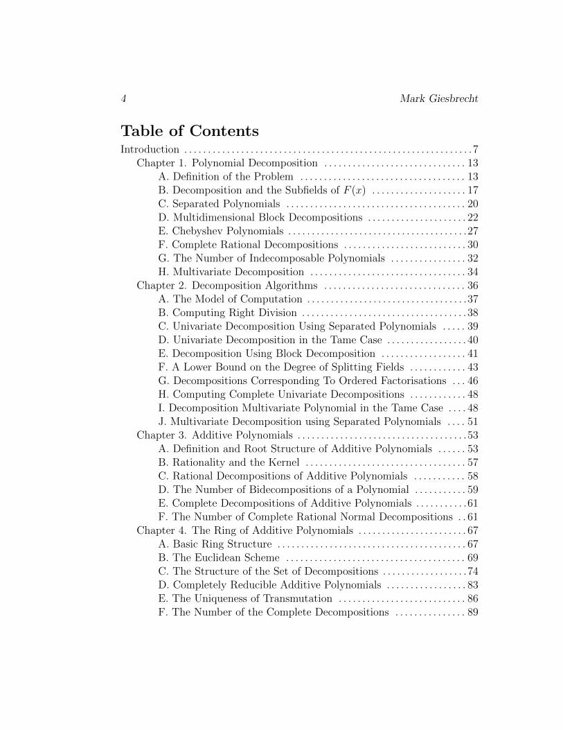
Table of ContentsIntroduction . . . . . . . . . . . . . . . . . . . . . . . . . . . . . . . . . . . . . . . . . . . . . . . . . . . . . . . . . . . . .7
Chapter 1. Polynomial Decomposition . . . . . . . . . . . . . . . . . . . . . . . . . . . . . . 13A. Definition of the Problem . . . . . . . . . . . . . . . . . . . . . . . . . . . . . . . . . . . 13B. Decomposition and the Subfields of F (x) . . . . . . . . . . . . . . . . . . . . 17C. Separated Polynomials . . . . . . . . . . . . . . . . . . . . . . . . . . . . . . . . . . . . . . 20D. Multidimensional Block Decompositions . . . . . . . . . . . . . . . . . . . . . 22E. Chebyshev Polynomials . . . . . . . . . . . . . . . . . . . . . . . . . . . . . . . . . . . . . .27F. Complete Rational Decompositions . . . . . . . . . . . . . . . . . . . . . . . . . . 30G. The Number of Indecomposable Polynomials . . . . . . . . . . . . . . . . 32H. Multivariate Decomposition . . . . . . . . . . . . . . . . . . . . . . . . . . . . . . . . . 34
Chapter 2. Decomposition Algorithms . . . . . . . . . . . . . . . . . . . . . . . . . . . . . . 36A. The Model of Computation . . . . . . . . . . . . . . . . . . . . . . . . . . . . . . . . . .37B. Computing Right Division . . . . . . . . . . . . . . . . . . . . . . . . . . . . . . . . . . . 38C. Univariate Decomposition Using Separated Polynomials . . . . . 39D. Univariate Decomposition in the Tame Case . . . . . . . . . . . . . . . . . 40E. Decomposition Using Block Decomposition . . . . . . . . . . . . . . . . . . 41F. A Lower Bound on the Degree of Splitting Fields . . . . . . . . . . . . 43G. Decompositions Corresponding To Ordered Factorisations . . . 46H. Computing Complete Univariate Decompositions . . . . . . . . . . . . 48I. Decomposition Multivariate Polynomial in the Tame Case . . . . 48J. Multivariate Decomposition using Separated Polynomials . . . . 51
Chapter 3. Additive Polynomials . . . . . . . . . . . . . . . . . . . . . . . . . . . . . . . . . . . .53A. Definition and Root Structure of Additive Polynomials . . . . . . 53B. Rationality and the Kernel . . . . . . . . . . . . . . . . . . . . . . . . . . . . . . . . . . 57C. Rational Decompositions of Additive Polynomials . . . . . . . . . . . 58D. The Number of Bidecompositions of a Polynomial . . . . . . . . . . . 59E. Complete Decompositions of Additive Polynomials . . . . . . . . . . .61F. The Number of Complete Rational Normal Decompositions . . 61
Chapter 4. The Ring of Additive Polynomials . . . . . . . . . . . . . . . . . . . . . . . 67A. Basic Ring Structure . . . . . . . . . . . . . . . . . . . . . . . . . . . . . . . . . . . . . . . . 67B. The Euclidean Scheme . . . . . . . . . . . . . . . . . . . . . . . . . . . . . . . . . . . . . . 69C. The Structure of the Set of Decompositions . . . . . . . . . . . . . . . . . .74D. Completely Reducible Additive Polynomials . . . . . . . . . . . . . . . . . 83E. The Uniqueness of Transmutation . . . . . . . . . . . . . . . . . . . . . . . . . . . 86F. The Number of the Complete Decompositions . . . . . . . . . . . . . . . 89

Functional Decomposition of Polynomials 5
Chapter 5. Decomposing Additive Polynomials . . . . . . . . . . . . . . . . . . . . . .90A. The Model of Computation . . . . . . . . . . . . . . . . . . . . . . . . . . . . . . . . . .90B. The Cost of Basic Operations in AF . . . . . . . . . . . . . . . . . . . . . . . . . . 91C. The Minimal Additive Multiple . . . . . . . . . . . . . . . . . . . . . . . . . . . . . .92D. Complete Rational Decomposition of Additive Polynomials . . 94E. General Rational Decomposition of Additive Polynomials . . . . 97F. General Decomposition of Completely
Reducible Additive Polynomials . . . . . . . . . . . . . . . . . . . . . . . . . . . . 100G. Determining Transmutations of Additive Polynomials . . . . . . 105H. Bidecomposition of Similarity Free Additive Polynomials . . . 107I. Absolute Decompositions of Additive Polynomials . . . . . . . . . . . 113
Chapter 6. Rational Function Decomposition . . . . . . . . . . . . . . . . . . . . . . 115A. The Normalised Decomposition Problem . . . . . . . . . . . . . . . . . . . 115B. Decomposing Normalised Rational Functions . . . . . . . . . . . . . . . 122
Conclusion. . . . . . . . . . . . . . . . . . . . . . . . . . . . . . . . . . . . . . . . . . . . . . . . . . . . . . . . .127References. . . . . . . . . . . . . . . . . . . . . . . . . . . . . . . . . . . . . . . . . . . . . . . . . . . . . . . . . 129

6 Mark Giesbrecht
Introduction.A fundamental idea in computer science and mathematics is that of compo-sition. One way to understand an object, whether it is abstract or concrete,is to understand how it combines with other objects of the same type. Aconverse problem to this also exists: Given an object, describe how it ismade up as the composition of other objects. This is decomposition. Wecan introduce constraints on the decompositions we wish to examine. Whathappens when we cannot further break down the object under considera-tion given these constraints? We say it is indecomposable. A very naturalquestion to look at is how an object under consideration breaks down intoindecomposable pieces. And if we relax the constraints somewhat, do theseindecomposable objects decompose once again? In mathematics, and espe-cially algebra, decomposition is a central concept. Decomposing matrices,algebras and groups are all well explored areas. The factoring of polynomialsis a fundamental example of the decomposition in the ring of polynomialsunder the usual operations of addition and multiplication. The computa-tional aspects of factoring polynomials have been an extremely active areaof research over the last two decades. But polynomials can also be com-posed functionally, and form a ring under addition and composition. Whatdoes factorisation in this ring look like? Although this question has been ad-dressed mathematically for at least six decades, many unresolved questionsstill remain. Computationally the area is extremely new, having developedonly over the last decade or so. Applications of polynomial decompositionwithin the areas of coding theory and cryptography exist (though will notbe dealt with here), and the problem is of computational interest in its ownright. Though some progress has been made in the (mathematically) wellunderstood cases, the problem in general appears to be difficult. We willaddress ourselves to some of these difficulties.
If fm, fm−1, . . . , f1 are univariate polynomials over a field F of degreesrm, rm−1, . . . , r1 ∈ N respectively, their functional composition
f = fm(fm−1(· · · (f2(f1)) · · ·)) ∈ F [x]
has degree n = rmrm−1 · · · r1, and can be computed in a straightforwardmanner. In this thesis we examine a converse problem. Namely, given fand rm, . . . , r1, determine if there exist polynomials fm, . . . , f1 ∈ F [x] suchthat deg fi = ri for 1 ≤ i ≤ m and f = fm(fm−1(· · · (f2(f1)) · · ·)), and

Functional Decomposition of Polynomials 7
if so, compute them. We call this the polynomial decomposition problem.When the problem is limited to decompositions into two composition factorsof given degree, we call this the bidecomposition problem. A polynomial isconsidered to be indecomposable if there is no way to decompose it into non-trivial (degree at least two) composition factors. We also consider decom-positions into indecomposable composition factors, which we call completedecompositions. Further questions arise when we consider decompositionsover arbitrary algebraic extension fields of the ground field, or absolute de-compositions. All these issues concerning decompositions have been dealtwith mathematically since the seminal paper of Ritt[1922], which showed avery strong, “well behaved” structure for decompositions of polynomials overthe complex numbers. Since then, the mathematical literature dealing withthe problem has been extensive, though far from complete. The difficulty inthe decomposition problem seems to be connected to the divisibility of thedegrees by the characteristic p of the ground field. The “tame” case, wherep = 0 or p - ri for 1 < i ≤ m is well understood. However, the “wild” casewhere p|ri for some i > 1 is still largely a mystery. It is this case in whichwe will be most interested.
For some special classes of polynomials, decompositions in the wild caseare well understood. One such class is the “additive” polynomials. These arethe polynomials where only exponents which are powers of the characteristicp of the field have non-zero coefficients. In some sense they are the “wildest”polynomials (see von zur Gathen[1988]). The theory of additive polynomi-als was introduced in Ore[1933b], and will be presented here in some detail.Kozen and Landau[1986] give an (exponential time) reduction of the generaldecomposition problem to univariate factorisation, and give a formulation ofthis problem in terms of the action of Galois groups. This turns out to besomewhat simpler for decompositions of separable, irreducible polynomials(over arbitrary fields) than in the general case. And for irreducible polyno-mials over finite fields they give a complete description of the decompositionstructure.
Decompositions of multivariate polynomials have also been considered.Evyatar and Scott[1972] show a structure very similar to the univariate case.We consider decompositions of a multivariate polynomial f into a univariatepolynomial g and a multivariate polynomial h. Completely analogous tameand wild cases exist, although even less is known about the wild case herethan for univariate polynomials.

8 Mark Giesbrecht
Computationally, polynomial decomposition has only been examined since1976 by Barton and Zippel[1976,1985]. They give a general algorithm (forboth the tame and wild cases) which requires a factoring subroutine and anexponential number of field operations in the degree of the input polynomial.Over arbitrary (“computable”) fields, the decomposition problem is undecid-able (see von zur Gathen[1988]). Kozen and Landau[1986] exhibit an algo-rithm for the bidecomposition problem in the tame case which requires onlya polynomial number of field operations in the input degree. For multivari-ate polynomials there is a similar situation. Fast algorithms which computedecompositions do exist in the tame case (see Dickerson[1987] and von zurGathen[1987]). And in the wild case we present an algorithm to performmultivariate decomposition (in an exponential number of field operations).Some special classes of the wild case have also been dealt with: Kozen andLandau[1986] give a decomposition algorithm for irreducible, separable poly-nomials which requires a quasi-polynomial number of field operations in thedegree of the input, and for irreducible polynomials over finite fields, theiralgorithm requires only a polynomial number of field operations in the inputdegree.
This thesis is organised into six chapters. In chapter one we present amathematical definition of the univariate decomposition problem and fivedifferent formulations of it. Each of these formulations has been used in themathematical or computational literature, in various forms. Some were de-veloped for special cases, and some fall immediately from the problem defini-tion. We generalise these formulations and put them in a consistent languageand context, showing their basic equivalence. We also define the multivariateproblem in a similar manner, showing two basic, equivalent formulations.
In chapter two, we present the computational approaches to polynomialdecomposition which have been developed for both the wild and tame cases.These algorithms will be stated in terms of the formulation of the decompo-sition problem used, as developed in chapter one. We show that for certain“nice” families of polynomials (polynomials for which an efficient algorithmfor decomposition into two composition factors of given degree exists, andfor which such decompositions are unique) the problem of decomposing apolynomial into an arbitrary number of factors of given degree is reducibleto the bidecomposition problem. Using a structure theorem of Evyatar andScott[1972], we also exhibit an algorithm for decomposing multivariate poly-nomials (in both the tame and wild cases) over any field supporting a fac-
Functional Decomposition of Polynomials 9
toring algorithm.In chapters three through five we introduce the additive polynomials, a
class of polynomials with wild decompositions which are well understood.In chapter three we develop the theory of these polynomials with respectto the structure of their roots in their splitting fields. From this we gar-ner quasi-polynomial lower bounds on the number of decompositions (bothdecompositions into two factors and complete decompositions) of “simple”additive polynomials. This shows that any algorithm which produces all de-compositions of an arbitrary polynomial in the wild case cannot be expectedto work in a polynomial number of field operations. In fact, we determine ex-actly the maximum number of decompositions of simple additive polynomialsof a given degree.
In chapter four the theory of Ore[1933a], which describes non-commutativeEuclidean rings, is developed for the additive polynomials. We extend thistheory by further developing the relationship between different complete de-compositions of a given polynomial. We also show a number of results con-cerning the uniqueness of decompositions. Combining this formal structurewith the algebraic structure from chapter three, we show a quasi-polynomialupper bound on the number of possible complete decompositions of additivepolynomials in general.
In chapter five we make use of the two previous chapters to develop al-gorithms for the decomposition of additive polynomials. We show that wecan determine indecomposability in a polynomial number of field operations,and in fact can generate one complete decomposition. However, the only waymethod we know to find a decomposition into an arbitrary number of factorsof given degrees is by finding all complete decompositions. Using the upperbound from chapter four, we get an algorithm requiring a quasi-polynomialnumber of field operations. Two large subclasses of the additive polynomialsshow more favourable results: the completely reducible additive polynomialsand the similarity free additive polynomials. Decomposition algorithms re-quiring a polynomial number of field operations are shown in each case. Wealso show a quasi-polynomial time algorithm for the absolute decompositionof additive polynomials. This algorithm may well run in a polynomial num-ber of field operations, subject to a conjectured (but unproven) upper boundon the degrees of splitting fields of additive polynomials. This conjecturefollows immediately from a much stronger (and also unproven) conjecture ofOre[1933b].

10 Mark Giesbrecht
In chapter six we define the rational function decomposition problem. Weshow a normalisation of this problem to a more a more uniquely defined form.We then show that the rational function decomposition problem is reducibleto this normal rational function decomposition problem. Finally, we presentan algorithm for solving the normal problem (in an exponential number offield operations in the input degree).
In summary the main original results of this thesis are:
(1) five equivalent formulations of the univariate decomposition problemand two formulations of the multivariate decomposition problem,
(2) a reduction from the general problem of finding decompositions intoan arbitrary number of factors of given degree to the bidecompositionproblem, for certain “nice” families of polynomials,
(3) an exponential time algorithm for decomposing multivariate polyno-mials (in both the tame and wild cases) over any field supporting afactoring algorithm,
(4) a precise determination of the maximum number of decompositions ofan additive polynomial (which is super-polynomial in the degree), giv-ing a super-polynomial lower bound on the number of decompositionsof a given polynomial in the wild case,
(5) a polynomial time algorithm for the complete decomposition of additivepolynomials, and hence an algorithm for determining indecomposabil-ity,
(6) a quasi-polynomial time algorithm for the decomposition of an additivepolynomial into factors of given degrees,
(7) polynomial time algorithms for the decomposition of two special classesof additive polynomials, the completely reducible additive polynomialsand the similarity free additive polynomials,
(8) a quasi-polynomial time algorithm for the absolute decomposition ofadditive polynomials, which could well run in polynomial time, subjectto an unproven conjecture of Ore[1933b],
(9) a definition of the rational function decomposition problem, as well asa normalised form of this problem, and a reduction from the generalproblem to the normal problem,

Functional Decomposition of Polynomials 11
(10) a computational solution to the normal rational function decompositionproblem, requiring an exponential number of field operations.
Results 5 through 8 assume the existence of a polynomial time algorithm forfactoring univariate polynomials.
12 Mark Giesbrecht
1 Polynomial Decomposition1.1 Definition of the ProblemLet F be an arbitrary field and K an extension field of F . A decompositionof a polynomial f ∈ F [x] is an ordered sequence of polynomials fi ∈ K[x]for 1 ≤ i ≤ m such that
f = fm(fm−1(· · · (f2(f1)) · · ·)= fm fm−1 · · · f2 f1.
If K = F then the decomposition is said to be rational. The polynomial f isconsidered to be (rationally) indecomposable if for any (rational) decompo-sition, all but one of the composition factors has degree one. If this is eventrue when K is allowed to be an algebraic closure of F , then f is absolutelyindecomposable.
Assume f = g h where f ∈ F [x] and g, h ∈ K[x]. Assume also that aand c are the leading (high order) coefficients of f and h respectively. Then
f
a= (
1
ag(cx+ h(0))) h− h(0)
c
is a decomposition of a monic polynomial into two monic polynomials, thesecond of which has constant coefficient zero. Thus, without loss of generality,we can assume for any decomposition f = gh that f, g, and h are monic andh(0) = 0. Similarly, if f = fm fm−1 · · · f1, we can assume that f ∈ F [x]and fi ∈ K[x] for 1 ≤ i ≤ m are monic and fi(0) = 0 for 1 ≤ i < m. Callany decomposition of this form a normal decomposition.
Define the rational normal decomposition problem as follows. For anyn,m ∈ N, an ordered factorisation of n of length m is an m-tuple
℘ = (rm, rm−1, . . . , r1)
where ri ∈ N and ri ≥ 2 for 1 ≤ i ≤ m and∏1≤i≤m
ri = n.
Let m ∈ N \ 0 and let F be any field of characteristic p, where p is a primenumber. Let PF = f ∈ F [x] : f monic. Define
DECF℘ =
(f, (fm, fm−1, . . . , f1)) ∈ PF × (PF )m∣∣∣∣∣f = fm fm−1 · · · f1
where deg fi = ri and
fi(0) = 0 for 1 ≤ i < m
.
Functional Decomposition of Polynomials 13
The computational problem is, given f ∈ PF and ℘ as above, to decidewhether there exist any
(fm, fm−1, . . . , f1) ∈ (PF )m
such that
(f, (fm, fm−1, . . . , f1)) ∈ DECF℘ ,
and in the affirmative case, to compute one or all of them.
The rational normal bidecomposition problem is a restriction of the aboveproblem to ordered factorisations ℘ = (r2, r1) of length two. Mathematically,this problem addresses many of the same questions as the general problemsince we can always look at decompositions into two parts, and then continuerecursively on the composition factors obtained. This problem has been ex-amined extensively in the literature, but many unresolved questions remain.Two basic cases emerge in the mathematical behaviour of the bidecomposi-tion problem. The “tame” case, when p - r2, is as its name might suggest,well behaved. Kozen and Landau[1986] observed that there exists at mostone decomposition for any given f and ℘ (this also follows from Fried andMacRae[1969a]). Furthermore, they showed it can be determined in poly-nomial time. As well, any normal decomposition of f will be rational inthis case. This was shown for the case F = C by Ritt[1922], for all fields ofcharacteristic zero by Levi[1942], and for the general “tame” case by Friedand MacRae[1969a].
The “wild” case, when p|r2, is much harder to deal with, both mathe-matically and computationally. Fields are exhibited over which the problemis undecidable in von zur Gathen[1988]. Decompositions are not necessar-ily unique as the following example shows (other examples can be found inOre[1933b]). Let F = GF (5). Then
f = x53 + x52 + x5 + x = (x52 + 3x5 + 2x) (x5 + 3x)
= (x52 + 4x5 + 3x) (x5 + 2x)
= (x52 + x) (x5 + x).
Here f has 3 distinct decompositions in DECF(52,5). Also, in the “wild” case
decompositions may not be rational. With F as above consider the polyno-

14 Mark Giesbrecht
mial
f = x52 + x5 + x
= (x5 + αx) (x5 + βx)
= x52 + (β5 + α)x5 + αβx.
It follows that α + β5 = αβ = 1, and the polynomial f has a decompositionof this form if and only if β is a root of ϕ = x6− x+ 1 ∈ F [x]. But ϕ has noroots in F , and hence f has monic normal decompositions only in algebraicextensions of F . It will be seen that even in small finite fields the number ofbidecompositions of a given polynomial of degree n can be super-polynomialin n. Polynomial time decomposition algorithms for rational decompositionsand for decompositions in algebraic extensions are known to exist only forcertain classes of polynomials.
The ring of polynomials F [x] under addition and composition is obviouslywithout zero divisors. It is not a (left or right) Euclidean ring however, asright or left division with remainder of f ∈ F [x] by g ∈ F [x] makes senseonly when the degree of g divides the degree of f .
Let F = GF (4), and let ω ∈ F be a primitive cube root of unity. Considerthe polynomial
f = (x4 − x)3 ∈ F [x].
Dorey and Whaples[1974] show
f = (x4 − x3 − x2 + x) (x3 + ωαx+ αω2)
for any α ∈ F . Hence left (compositional) division of f by (x4 − x3 −x2 + x) is not unique. A somewhat stronger statement can be made about(compositional) right division. Let F be an arbitrary field andK an extensionfield of F .
Lemma 1.1. If f, h ∈ F [x] and g ∈ K[x] are nonzero of degrees n, r and srespectively, and f = g h, then
(i) g is uniquely determined by f and h, and
(ii) g ∈ F [x].
Proof.
Functional Decomposition of Polynomials 15
(i) Assume g′ ∈ K[x] is such that f = g′ h. Then
0 = g h− g′ h= (g − g′) h,
and as F [x] under composition has no zero divisors, this implies thatg = g′.
(ii) The coefficients of f are K-linear combinations of the coefficients of hi
for 1 ≤ i ≤ r. The coefficients of f and hi are in F , so the coefficientsof g are a solution to a system of linear equations over F . Since such asystem has a solution in F if it has one over K, and g is unique by (i),the coefficients of g are in F and g ∈ F [x].
Further structure can be derived about the fields over which decomposi-tions exist. Let F be a field and let F be a fixed algebraic closure of F .
Lemma 1.2. Let f, g, h ∈ F [x] have degrees n, r, and s respectively andf = g h. Assume f has splitting field K ⊆ F . Then g splits over K and foreach root α ∈ K of g, h− α splits over K.
Proof. Assume
g =∏
1≤i≤r(x− βi)
where βi ∈ F for 1 ≤ i ≤ r. Then
f =∏
1≤i≤r(h− βi).
Let γ = βi for some i ∈ N with 1 ≤ i ≤ r. If α ∈ F is a root of h− γ, then αis a root of f . Hence α ∈ K and h− γ splits over K. Since γ is the productof the roots of h− γ, γ ∈ K. Therefore, g splits over K as well.
This theorem implies a number of interesting facts about decompositionsover extensions of the ground field.
Corollary 1.3. Let F be an arbitrary field and L ⊇ F an extension field.Let f ∈ F [x] be monic of degree n with splitting field K. Then, if f isindecomposable in K, f is indecomposable in L.

16 Mark Giesbrecht
Proof. Suppose f = g h for some g, h ∈ L[x] whose degrees are at leasttwo. Then, by lemma 1.2, g splits in K, so g ∈ K[x]. Let γ ∈ K be a rootof g. Then h− γ splits over K (also by lemma 1.2) and h ∈ K[x]. But f isindecomposable over K and we get a contradiction.
Decomposition over an arbitrary field extension (or decomposition in thesplitting field as just shown) is called absolute decomposition. We will see intheorem 2.8 that over many fields F there are polynomials f ∈ F [x] whosesplitting fields are of degree exponential in n over F . Over infinite fields Fvon zur Gathen [1987a] showed that there exist polynomials of degree n suchthat the coefficients of an absolute decomposition generate a field extensionof degree exponential in n over F . It is conjectured that such examples existover finite fields as well.
1.2 Decomposition and the Subfields of F (x).The decompositions of a polynomial f ∈ F [x] have a strong correspondencewith the lattice of subfields between F (f) and F (x), where F (x) is an al-gebraic extension over F (f) of the same degree as the degree of f (see vander Waerden[1970] section 10.2). This was first examined by Levi[1942] andlater by Fried and MacRae[1969a,b]. Let n ∈ N and ℘ = (rm, rm−1, . . . , r1)be an ordered factorisation of n. Let L be the set of all subfields of F (x).Define
FIELDSF℘ =
(f, (Fm, . . . , F1)) ∈ PF × Lm∣∣∣∣∣Fm = F (f), F0 = F (x),
Fm ⊆ Fm−1 ⊆ · · · ⊆ F1 ⊆ F0,
[Fi−1 : Fi] = ri, 1 ≤ i ≤ m
where [Fi−1 : Fi] is the algebraic degree of Fi−1 over Fi.
Let f ∈ F [x] be of degree n. Also, let (f, (fm, fm−1, . . . , f1)) ∈ DECF℘
and for 1 ≤ i ≤ m let hi = fi fi−1 · · · f1 and Fi = F (hi), the field F withhi adjoined. Define ΓD
F : DECF℘ → FIELDSF℘ by (f, (fm, fm−1, . . . , f1)) 7→
(f, (Fm, Fm−1, . . . , F1)). This is a map into FIELDSF℘ by the fact that [Fi−1 :Fi] = ri.
Theorem 1.4. ΓDF is a bijection.
Proof. Different decompositions give rise to different chains of fields becausefor any hi, h
′i ∈ F [x], F (hi) = F (h′i) if and only if hi = ah′i + b for some
Functional Decomposition of Polynomials 17
a, b ∈ F , a 6= 0. If hi, h′i ∈ F [x] are monic with hi(0) = h′i(0) = 0, this
implies hi = h′i. Thus ΓDF is injective.
Showing that ΓDF is surjective is somewhat less trivial. Let f ∈ F [x] be
monic of degree n. Then F (x) is a finite extension of F (f) of degree n. LetL be a field such that F (f) ⊆ L ⊆ F (x). Then L = F (h) for some h ∈ F (x).Since h generates L over F and f ∈ L, f = g h for some g ∈ F [x]. Thus his a root of f − g(y) ∈ F (x)[y]. Since f − g(y) is also in F [x, y], all roots inF (x) must be in F [x] (see van der Waerden[1970] section 5.4) and h ∈ F [x].As F (ah+ b) = F (h) for a, b ∈ F and a 6= 0, we can assume h is monic withh(0) = 0. Assume h′ ∈ F [x] is also monic with h′(0) = 0 and L = F (h′).We know h′ and h have the same degree, that is [F (x) : L], and becauseh′ ∈ F (h), h′ = ch + d for some c, d ∈ F , c 6= 0. But both are monic withconstant coefficient zero, so h = h′ and h is unique. Assume h has degrees. The field L is an algebraic extension of F (f) of degree r = n/s, and thedegree of g ∈ F [x] is r.
Now assume (f, (Fm, Fm−1, . . . , F1)) ∈ FIELDSF℘ . Let hi ∈ F [x] withhi(0) = 0 be the unique monic generator of Fi as above. Because F (hi−1) ⊇F (hi), we know hi = fi hi−1, for some (unique) fi ∈ F [x], for 1 ≤ i <m. The degree of F (hi−1) over F (hi) is ri, so the degree of fi is ri. Be-cause f may have a non-zero constant term, f = hm + c, where c ∈ Fis the constant term of f . As before, F (hm−1) ⊇ F (hm) so there ex-ists a unique fm of degree rm such that hm = fm hm−1. Letting fm =fm + c, it follows that (f, (fm, fm−1, . . . , f1)) ∈ DECF
℘ . It is easily seen thatΓDF (f, (fm, fm−1, . . . , f1)) = (f, (Fm, Fm−1, . . . , F1)) and so ΓD
F is surjectiveand hence bijective.
Let f ∈ F [x] be separable of degree n (ie. ∂∂xf 6= 0). In the separable
case we can study the lattice of fields between F (f) and F (x) by looking atthe Galois group of F (x) relative to F (f). This was first done in Dorey andWhaples[1974] for the set of additive polynomials (a subset of F [x] whichwill be dealt with in detail in a later section). As F (x) is not necessarily anormal, separable, extension of F (f), we construct the splitting field Ω ofthe minimal polynomial of x over F (f). This minimal polynomial is
Φf (y) = f(y)− f ∈ F (f)[y] ⊆ F (x)[y] ,
since we know that x has degree n over F (f) and x satisfies Φf which also hasdegree n. Because f is separable, Φf is separable, so the field Ω is a normal,

18 Mark Giesbrecht
separable, extension of F (f) containing F (x). Let Gf = Gal(Ω/F (f)), theGalois group of Ω relative to F (f), and let Gx ⊆ Gf be the subgroup fixingF (x) pointwise. Let G be the set of all subgroups of Gf . For n ∈ N and℘ = (rm, rm−1, . . . , r1), an ordered factorisation of n, define
GROUPSF℘ =
(f, (Gm, . . . ,G1)) ∈ PF × Gm∣∣∣∣∣Gm = Gf , G0 = GxGm ⊇ Gm−1 ⊇ · · · ⊇ G1 ⊇ G0
(Gi : Gi−1) = ri, 1 ≤ i ≤ r
where (Gi : Gi−1) is the index of Gi−1 in Gi.
Let f ∈ F [x] be separable of degree n and let (f, (Fm, Fm−1, . . . , F1)) ∈FIELDSF℘ . As above, let Ω be the splitting field of Φf and let Gf =Gal(Ω/F (f)). For 1 ≤ i ≤ m let Gi ⊆ GF be the group of automorphismsfixing Fi pointwise. Define ΓF
G : FIELDSF℘ → GROUPSF℘ by
(f, (Fm, Fm−1, . . . , F1)) 7→ (f, (Gm,Gm−1 . . . ,G1)).
This map is simply the one described in the fundamental theorem of Galoistheory (see van der Waerden[1970] section 8.1-8.3).
Theorem 1.5. If f is separable then ΓFG is a bijection.
Proof. By the fundamental theorem of Galois theory, there is an inclusioninverting bijection between fields between F (x) and F (f) and groups betweenGx and Gf . An automorphism group H such that Gx ⊆ H ⊆ Gf correspondsto the field L such that F (x) ⊇ L ⊇ F (f) which it leaves fixed pointwise.Thus each chain of fields
F (f) = Fm ⊆ Fm−1 ⊆ · · · ⊆ F1 ⊆ F (x)
corresponds uniquely to a tower of groups
Gf = Gm ⊇ Gm−1 ⊇ · · · ⊇ G0 = Gx.
Also by the fundamental theorem, (Gi : Gi−1) = [Fi−1 : Fi] = ri. As ΓFG is
exactly this Galois mapping, the fact that it is a bijection follows immedi-ately.

Functional Decomposition of Polynomials 19
1.3 Separated PolynomialsFrom the correspondence between decompositions and fields between F (f)and F (x) we get a useful structural result. This was originally due toFried and MacRae[1969b] and was later extended to the multivariate caseby Evyatar and Scott (this will be dealt with in a subsequent section).Fried and MacRae[1969b] introduce a more general version of the polyno-mials Φf = f(y) − f(x) ∈ F (f)[y] and Φh = h(x) − h(y) ∈ F (h)[y] pre-viously described. Let F be an arbitrary field with independent indetermi-nates x and y over F . A polynomial Υ ∈ F [x, y] is said to be separated ifΥ(x, y) = f1(x)− f2(y) where f1, f2 ∈ F [x]. They then showed the followingtheorem linking separated polynomials with the simultaneous bidecomposi-tion of two polynomials with a common left composition factor:
Fact 1.6. Let f1, f2, h1, h2 ∈ F [x]. Then h1(x) − h2(y)|f1(x) − f2(y) if andonly if there exists a polynomial g ∈ F [x] such that f1 = gh1 and f2 = gh2.
If we let f1 = f2 and h1 = h2 we immediately have the following corollary:
Corollary 1.7. Let f, h ∈ F [x] be monic of degrees n and s respectivelywith h(0) = 0. The following are equivalent:
(i) There exists a g ∈ F [x] such that f = g h.
(ii) Φh|Φf .
We can now apply this theorem to get another formulation of generaldecompositions. Let S = h(x) − h(y) ∈ F [x, y] : h ∈ PF. Let n ∈ N and℘ = (rm, rm−1, . . . , r1), an ordered factorisation of n. Also, let di =
∏1≤j≤i rj.
Define
SEP F℘ =
(f, (Φm,Φm−1 . . . ,Φ1)) ∈ PF × Sm
∣∣∣ degx Φi = di, Φm = Φf
Φi|Φi+1 for 1 ≤ i < m
.
Let (f, (fm, fm−1, . . . , f1)) ∈ DECF℘ and, for 1 ≤ i ≤ m, let
ui = fi fi−1 · · · f1(x)− fi fi−1 · · · f1(y) ∈ F [x, y].
By corollary 1.7, ui|ui+1. Define the map ΓDS : DECF
℘ → SEP F℘ by
(f, (fm, fm−1, . . . , f1)) 7→ (f, (um, um−1 . . . , u1)).

20 Mark Giesbrecht
Theorem 1.8. ΓDS is a bijection.
Proof. As distinct decompositions will give a distinct sequences of ui’s for1 ≤ i ≤ m, this is an injective mapping from DECF
℘ to SEP F℘ .
Now assume (f, (vm, vm−1, . . . , v1)) ∈ SEP F℘ where vi(x, y) = gi(x)−gi(y)
for 1 ≤ i ≤ m. By corollary 1.7, we know that for 1 < i ≤ m, gi = fi gi−1
for some fi ∈ F [x] of degree ri. Thus (f, (fm, fm−1, . . . , f3, f2, g1)) ∈ DECF℘ .
Each member of SEP F℘ will be mapped to a different member of DECF
℘ sothere is an injection from SEP F
℘ to DECF℘ . This is obviously the inverse of
ΓDS , and so ΓD
S is a bijection.
1.4 Multidimensional Block Decompositions
Kozen and Landau[1986] developed another formulation of the bidecomposi-tion of a polynomial f ∈ F [x] based on its Galois group Gf , and this group’saction on the roots of f in its splitting field. The roots are partitioned byGf into blocks or systems of imprimitivity (see van der Waerden[1970], sec-tion 7.9). A necessary and sufficient condition in terms of these blocks isgiven for there to be a corresponding bidecomposition of f . We extend thisformulation to general decompositions of f corresponding to a given orderedfactorisation ℘.
Let U be a set. A multiset S over U is any map S : U → N. An elementα ∈ U is an element of S (α ∈ S) if and only if S(α) > 0. A multiset can beviewed as an extension of the characteristic function of a set. A multiset Tis a submultiset of a multiset S (T ⊆ S) if for all α ∈ U , T (α) ≤ S(α). Ifσ : U → U is a map, we consider the multiset σS to be defined such that forall α ∈ U
(σS)(α) =∑β∈Sσβ=α
S(β).
The cardinality of a multiset S is
|S| =∑α∈S
S(α).
At first reading, the reader is encouraged to think of multisets as sets S ⊆ U(or equivalently, as the characteristic functions of sets); if the polynomial fto be decomposed is squarefree, indeed only such sets will occur.

Functional Decomposition of Polynomials 21
We will see that decompositions into, say, three composition factors, cor-respond in a natural way to certain “multisets of multisets of multisets ofroots”. We introduce these “typed” objects over some set U as follows. Amultiset with one level over U is a multiset over U and, for i > 1, a multisetwith i levels over U is a multiset over the set of multisets with i − 1 levelsover U . Let B be a multiset with m levels over U . A multiset C is a level kmember of B if
C ∈ Bk−1 ∈ · · · ∈ B1 ∈ B.
Notice that the structure of B implies that C must be a multiset with m− klevels. C also has a natural multiplicity within B, namely
B(B1) ·B1(B2) · · ·Bk−2(Bk−1) ·Bk−1(C).
This allows us to “flatten” the top k levels of B and speak of the multiset ofall multisets at level ` in B. We denote this multiset with m − k + 1 levelsas B[`].
Let m ∈ N and ℘ = (rm, rm−1, . . . , r1) ∈ Nm. A multiset B with m levelsover U is a ℘-block if either
(i) m = 1 and B is a multiset over U of cardinality r1, or
(ii) m > 1 and B is a multiset with cardinality rm of (rm−1, rm−2, . . . , r1)-blocks over U .
Let BF be the set of all multisets with i levels over F for all i > 0, where Fis a fixed algebraic closure of F . Define the set
BLOCKSF℘ =
(f,B) ∈ PF × BF∣∣∣∣∣
B is a ℘-block over F such that
f =∏
α∈B[m]
(x− α)B[m](α)
.Let f ∈ F [x] be of degree n with splitting field K ⊆ F and Galois groupGf = Gal(K/F ) and let ℘ = (rm, rm−1, . . . , r1) be an ordered factorisationof n. A ℘-block B over K is a ℘-block decomposition of f if
(i) f =∏
α∈B[m]
(x− α)B[m](α), and
(ii) for any α, β ∈ B[m] and σ ∈ Gf such that σα = β, and for 1 ≤ ` < mand any C,D over K with C,D ∈ B[m−`] such that α ∈ C [`] and β ∈ D[`],it is true that σC [`] = D[`].

22 Mark Giesbrecht
A ℘-block decomposition is said to be functional if there exist monic poly-nomials h1, h2, . . . , hm−1 ∈ F [x] such that for 1 ≤ ` < m, h`(0) = 0 and forall C ∈ B[m−`] there exists a γC ∈ K such that
∏α∈C[`]
(x− α)C[`](α) = h` + γC.
Define
FBLOCKSF℘ =
(f,B) ∈ PF × BF
∣∣∣ B is a functional ℘-block
decomposition of f
.
Note that FBLOCKSF℘ ⊆ BLOCKSF℘ .We now give an example of a ℘-block decomposition. Let p ∈ N be prime
and let F = GF (p). Let f ∈ F [x] be irreducible of degree n = 12 withsplitting field K = F [z]/(f) and Galois group Gf = Gal(K/F ) = σj :
x → xpi
for 0 ≤ j < 12. We will exhibit a block decomposition of f inBLOCKSF℘ , where ℘ is the ordered factorisation (2, 3, 2). Since F is finite
and f is irreducible, f has roots α, αp, αp2 , . . . , αp11 ⊆ K. First, we finda block decomposition B of f in BLOCKSF(6,2). Let B = C0, C1, . . . , C5,where Ci = αpi , αpi+6 for 0 ≤ i < 6. Condition (i) of the definition of a℘-block trivially holds. If, for 0 ≤ i, j, k < 12, σkα
pi = αpi+k
= αpj, then
i + k ≡ j mod 12 and σkαpi+6
= αpi+6+k
= αpj+6
for 0 ≤ i, j, k < 12 sincei+ 6 + k ≡ j + 6 mod 12. Thus, condition (ii) in the definition holds as well.In a similar way we find that A = D0, D1 where Di = α2j+i : 0 ≤ j < 5for 0 ≤ i < 2 is a decomposition of f in BLOCKSF(2,6). Combining these twodecomposition, it follows that
E =α, αp6, αp2 , αp8, αp4 , αp10 , αp, αp7, αp3 , αp9, αp5 , αp11
is a block decomposition of f in BLOCKSF(2,3,2).
We now proceed to describe a bijective map ΓDB fromDECF
℘ to FBLOCKSF℘ .We first define ΓD
B from DECF℘ to BLOCKSF℘ . We then show it is a map to
FBLOCKSF℘ , and finally that it is bijective.Once again, let n,m ∈ N and ℘ = (rm, rm−1, . . . , r1), an ordered factori-
sation of n. Also, let (f, (fm, fm−1, . . . , f1)) ∈ DECF℘ , where f ∈ F [x] has
splitting field K. We define the map ΓDB recursively as follows. If m = 1, let
Functional Decomposition of Polynomials 23
B be the multiset of roots of f . It follows immediately that B is a ℘-blockof the roots of f in K, so we let ΓD
B(f, (f)) = (f,B).Now assume m > 1. We know f = fm hm−1 where h` = f`−1 f`−2
· · · f1 ∈ F [x] for 1 ≤ ` ≤ m. Let Dm be the multiset of roots of fm in K(we know they are in K by lemma 1.2). Then
f =∏
α∈Dm(hm−1 − α)Dm(α).
For each α ∈ Dm, let Eα = ΓDB(hm−1 − α, (fm−1 − α, fm−2, fm−3, . . . , f1)),
an (rm−1, rm−2, . . . , r1)-block over K of the roots in K of hm−1 − α by therecursive definition. For each (rm−1, rm−2, . . . , r1)-block C over K, define themultiset B such that
B(C) =
Dm(α) if C = Eα for some α ∈ Dm,
0 otherwise.
B is the multiset of the Eα’s (for all α ∈ Dm) with appropriate multiplicity.This is a ℘-block over K of the roots of f and hence (f,B) ∈ BLOCKSF℘ .We therefore define ΓD
B(f, (fm, fm−1, . . . , f1)) = (f,B). We have completelydescribed the map ΓD
B : DECF℘ → BLOCKSF℘ .
Lemma 1.9. ΓDB is a map from DECF
℘ to FBLOCKSF℘ .
Proof. Let (f, (fm, fm−1, . . . , f1)) ∈ DECF℘ and let (f,B) be its image in
BLOCKSF℘ under ΓDB . It follows immediately that (f,B) is functional from
the definition of ΓDB . We must also show that condition (ii) in the definition
of ℘-block decomposition holds for (f,B).Assume α, β ∈ B[m] and σ ∈ Gf such that σα = β. Let ` ∈ N such that
1 ≤ ` < m and let C,D ∈ B[m−`]. We know∏a∈C[`]
(x− a)C[`](a) = h` + γ,
∏b∈D[`]
(x− b)D[`](b) = h` + δ,
for some γ, δ ∈ K by the definition of ΓDB . Since
0 = σ(h`(α) + γ)
= h`(σα) + σγ
= h`(β) + σγ

24 Mark Giesbrecht
and h`(β) + δ = 0, we also know δ = σγ. Furthermore, since
σ(h` + γ) = σ∏
a∈C[`]
(x− a)C[`](a)
=∏
a∈C[`]
(x− σa)C[`](a),
andσ(h` + γ) = h` + δ
=∏
b∈D[`]
(x− b)D[`](b),
there is a bijection between the linear factors (over K) of h` + γ and h` + δ.As there is a trivial bijection between the linear factors of a polynomial overits splitting field and the multiset of roots of that polynomial, σC [`] = D[`].Therefore ΓD
B is a map from DECF℘ to FBLOCKSF℘ .
Theorem 1.10. ΓDB is a bijection.
Proof. ΓDB is an injection since each different decomposition gives a different
sequence h1, h2, . . . , hm, and hence a different block decomposition. We nowshow it is also surjective by induction on m. Let (f,B) ∈ FBLOCKSF℘ . Ifm = 1 then B is simply the multiset of roots of f and ΓD
B(f, (f)) = (f,B).Assume m is greater than one. Then
f =∏
α∈B[m]
(x− α)B[m](α)
=∏D∈B
(∏
α∈D[m−1]
(x− α)D[m−1](α))B(D)
=∏D∈B
(hm−1 − γD)B(D)
=∏D∈B
(x− γD)B(D) hm−1
for some γD ∈ K for each D ∈ B. It follows that there exists a polynomialfm ∈ K[x] such that
fm =∏D∈B
(x− γD)B(D)
Functional Decomposition of Polynomials 25
and f = fm hm−1. By lemma 1.1, fm ∈ F [x] and this fm is unique. Nowlet C ∈ B[m−`] for any ` with 1 < ` < m. Then∏
α∈C[`]
(x− α)C[`](α) = h` − δ for some δ ∈ K
=∏D∈C
(∏
α∈D[`−1]
(x− α)D[`−1](α))C(D)
=∏D∈C
(h`−1 − γD)C(D)
=∏D∈C
(x− γD)C(D) h`−1
for some γD ∈ K for each D ∈ C. So there exists a polynomial g` ∈ K[x]such that
g` =∏D∈C
(x− γD)C(D)
and h` − δ = g` h`−1. Rearranging this, h` = (g` + δ) h`−1 and by lemma1.1, f` = g` + δ ∈ F [x] and this f` is unique. This shows h` = f` h`−1 forsome uniquely determined f` ∈ F [x] for 1 < ` < m.
It follows that f = fmfm−1· · ·f3f2h1 where fi ∈ F [x] is monic of de-gree ri for 1 < i ≤ m and deg h1 = r1. Therefore (f, (fm, fm−1, . . . , f3, f2, h1)) ∈DECF
℘ and ΓDB(f, (fm, fm−1, . . . , f3, f2, h1)) = (f,B). This means that ΓD
B issurjective and hence bijective.
1.5 Chebyshev PolynomialsThe Chebyshev polynomials, Ti ∈ C[x] for i ∈ N, are usually defined over thecomplex numbers by the identity
Ti(cos θ) = cos iθ.
From the trigonometric identity
cos θ1 + cos θ2 = 2 cos
(θ1 + θ2
2
)cos
(θ1 − θ2
2
),
we getcos iθ + cos((i− 2)θ) = 2 cos((i− 1)θ) cos θ
26 Mark Giesbrecht
and
Ti(cos θ) + Ti−2(cos θ) = 2 cos θTi−1(cos θ).
This gives the defining recurrence relation
T0 = 1,
T1 = x,
Ti = 2xTi−1 − Ti−2, (i > 1)
so thatT2 = 2x2 − 1,
T3 = 4x3 − 3x,
T4 = 8x4 − 8x2 + 1,
...
Note that Ti ∈ Z[x] for all i ∈ N, so Chebyshev polynomials are in factwell defined (by this recurrence) in arbitrary fields of arbitrary characteris-tic, and have coefficients in the prime field of this characteristic. We willprove a number of useful theorems concerning Chebyshev polynomials overarbitrary fields. Obviously, no analytic properties of trigonometric functionshave meaning in fields of positive characteristic, so we will not make use ofany of these.
If F has characteristic two, then
T0 = 1,
T1 = x,
Ti = Ti−2 for i > 2.
Therefore Ti = 1 if i is even and Ti = x if i is odd.Let F be any field of characteristic p 6= 2, and for i ∈ N, let Ti be the
ith Chebyshev polynomial. A quick examination of the defining recurrencereveals that deg Ti = i.
Theorem 1.11.
Ti
(x+ x−1
2
)=xi + x−i
2.
Functional Decomposition of Polynomials 27
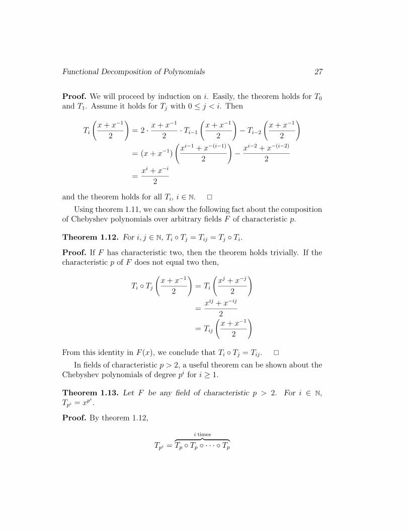
Proof. We will proceed by induction on i. Easily, the theorem holds for T0
and T1. Assume it holds for Tj with 0 ≤ j < i. Then
Ti
(x+ x−1
2
)= 2 · x+ x−1
2· Ti−1
(x+ x−1
2
)− Ti−2
(x+ x−1
2
)
= (x+ x−1)
(xi−1 + x−(i−1)
2
)− xi−2 + x−(i−2)
2
=xi + x−i
2
and the theorem holds for all Ti, i ∈ N.
Using theorem 1.11, we can show the following fact about the compositionof Chebyshev polynomials over arbitrary fields F of characteristic p.
Theorem 1.12. For i, j ∈ N, Ti Tj = Tij = Tj Ti.
Proof. If F has characteristic two, then the theorem holds trivially. If thecharacteristic p of F does not equal two then,
Ti Tj(x+ x−1
2
)= Ti
(xj + x−j
2
)
=xij + x−ij
2
= Tij
(x+ x−1
2
)
From this identity in F (x), we conclude that Ti Tj = Tij.
In fields of characteristic p > 2, a useful theorem can be shown about theChebyshev polynomials of degree pi for i ≥ 1.
Theorem 1.13. Let F be any field of characteristic p > 2. For i ∈ N,Tpi = xp
i.
Proof. By theorem 1.12,
Tpi =
i times︷ ︸︸ ︷Tp Tp · · · Tp

28 Mark Giesbrecht
so it is sufficient to show Tp = xp. We know
Tp
(x+ x−1
2
)=xp + x−p
2
=
(x+ x−1
2
)p.
From this identity in F (x), we conclude that Tp = xp.
1.6 Complete Rational Decompositions
A complete rational decomposition of a polynomial f ∈ F [x] is of the form
f = fm fm−1 · · · f2 f1
where each fi ∈ F [x] is indecomposable and nontrivial (ie. with degreegreater than one). A natural question to ask concerns the uniqueness of suchdecompositions. As we do not want to worry about affine linear transfor-mations of composition factors, we consider only complete rational normaldecompositions where f is monic and fi ∈ F [x] are monic for 1 ≤ i ≤ m andfi(0) = 0 for 1 ≤ i < m.
Two types of ambiguous decompositions emerge. If u ∈ F [x], then (xm ·ur)xr = xr(xm ·u(xr)) for m, r ∈ N. Call this an exponential ambiguity. Asseen in the previous section, the Chebyshev polynomials Ti ∈ F [x] for i ∈ Nhave the property that Ti Tj = Tj Ti. Call this a trigonometric ambiguity.Ritt[1922] showed that if F = C, all complete normal decompositions differonly by ambiguities of these two forms. Engstrom[1941] showed that in fieldsF of characteristic zero that
(i) polynomials indecomposable over F are indecomposable over any alge-braic extension of F (ie. all decompositions are rational), and
(ii) all complete normal decompositions differ only by trigonometric andexponential ambiguities.
These two theorems are known as Ritt’s first and second theorems. Friedand MacRae[1969a] showed them true when the characteristic of F is greaterthan the degree of the polynomial.

Functional Decomposition of Polynomials 29
For an arbitrary field F of characteristic p this is not necessarily true.Dorey and Whaples[1974] give the following example of two complete rationaldecompositions of the polynomial f ∈ F [x]:
f = xp3+p2 − xp3+1 − xp2+p + xp+1
= xp+1 (xp + x) (xp − x)
= (xp2 − xp2−p+1 − xp + x) xp+1.
The composition factor xp2−xp2−p+1−xp +x is indecomposable because the
composition of two polynomials of degree p can never have a term of degreep2 − p+ 1.
The various equivalent formulations to polynomial decompositions canbe extended to complete decompositions in the obvious manner. Let ℘ bean ordered factorisation of n of length m. Let cDECF
℘ ⊆ DECF℘ be the set
of complete decompositions of polynomials corresponding to ordered factori-sation ℘. The image of cDECF
℘ in FIELDSF℘ , GROUPSF℘ , SEP F℘ , and
FBLOCKSF℘ under the bijections described in this chapter will be called,respectively, cFIELDSF℘ , cGROUPSF℘ , cSEP F
℘ and cBLOCKSF℘ . Obvi-ously, any member of any one of these sets will correspond to a completerational normal decomposition.
The sets cFIELDSF℘ and cGROUPSF℘ have useful characterisations intheir own right. If (f, (Fm, Fm−1, . . . , F1)) ∈ cFIELDSF℘ , then
F (f) = Fm ⊆ Fm−1 ⊆ · · · ⊆ F1 ⊆ F (x)
is a maximal chain of fields. If a field did exist between Fi and Fi+1 then fi+1,the i + 1’st composition factor from the corresponding element(f, (fm, fm−1, . . . , f1)) ∈ cDECF
℘ , would be decomposable. In a similar fash-ion, if (f, (Gm,Gm−1, . . . ,G1)) ∈ cGROUPSF℘ , then
Gx ⊆ G1 ⊆ · · · ⊆ Gm−1 ⊆ Gm = Gf
is a maximal tower of groups.When dealing with complete decompositions of a polynomial f ∈ F [x],
we often wish to deal with all decompositions of f regardless of the orderedfactorisations to which they correspond. With this in mind we define
cDECF∗ =
⋃℘∈T
cDECF℘ .

30 Mark Giesbrecht
where T is the set of all finite tuples of integers greater than one. Similarly wecan define cFIELDSF∗ , cGROUPSF∗ , etc, and restate Ritt’s second theoremin this context: For any monic f ∈ F [x], all decompositions of f in cDECF
∗are equivalent up to trigonometric and exponential ambiguities.
1.7 The Number of Indecomposable PolynomialsIt can shown that “most” polynomials over an arbitrary field F are indecom-posable. This can be done using an algebraic dimension argument over analgebraically closed field and by a counting argument over a finite field.
Let F be a field, and M ⊆ F [x] be the set of monic polynomials withconstant coefficient zero. Also, for n ∈ N, let Mn = f ∈ M | deg f = nand for r, s ∈ N with rs = n and g ∈ Mr and h ∈ Ms, define α(r,s) : Mr ×Ms → Mrs by α(r,s)(g, h) = g h (ie. the composition function). Assumef =
∑0≤i≤n aix
i ∈ Mn where ai ∈ F for 0 ≤ i ≤ n. We define the mapλn : Mn → F n−1 by λn(f) = (an−1, an−2, . . . , a1). This is obviously a bijectivemap from Mn to F n−1. Assume r and s are at least two and define β(r,s) :F r−1×F s−1 → F n−1 by β(r,s) = λnα(r,s)(λ−1
r ×λ−1s ). This is the composition
map in F n−1. Let
D(r,s) = β(r,s)(A,B) ∈ F n−1 |A ∈ F r−1, B ∈ F s−1
be the image of β(r,s) in F n−1. We will show that the “size” of F n−1 is “muchlarger” than the “size” of
D =⋃rs=n
D(r,s),
the set of all decomposable polynomials in Mn. Because we can normaliseany decomposition, this is in fact a general statement about the number ofindecomposable polynomials in F [x].
Consider the case where F is an algebraically closed field. For r, s ∈ Nwith rs = n and r > 1, D(r,s) (the Zariski closure of D(r,s)) is an algebraicset of dimension at most r + s− 2. Therefore
D =⋃rs=nr,s>1
D(r,s)
has dimension at most
maxdim D(r,s) : rs = n, r, s > 2 ≤ n
2

Functional Decomposition of Polynomials 31
and this is less than the dimension n−1 of F n−1. Therefore, over an arbitraryinfinite field, “most” polynomials are indecomposable even over an algebraicclosure of that field, in a strong algebraic sense.
Turning to the case F = GF (q) where q = pi for some prime number p andi ∈ N, we can make a counting argument to show that only an exponentiallysmall number of polynomials in F [x] of degree n are decomposable. For anyordered factorisation (r, s) of n with s > 1, we know #D(r,s) ≤ qr−1qs−1 =qr+s−2. Summing over all possible ordered factorisation (r, s) of n wheres > 1, we get
#D ≤∑rs=n
qr+s−2
≤ d(n)q2+n/2−2
≤ d(n)qn/2
.
where d(n) is the number of divisors of n. From Hardy and Wright[1960](theorem 317) we get d(n) ≤ cεn
ε for any ε > 0 and some cε > 0 (dependingon ε). Fixing an ε > 0,
#D ≤ cεqn2
≤ cεqε logq n+n
2
≤ kq2n/3.
for some k > 0. This shows that only an exponentially small fraction of thepolynomials of degree n over GF (q) are decomposable.
1.8 Multivariate DecompositionLet F be an arbitrary field and let x, x1, . . . , x`, y, y1, . . . , y` be algebraicallyindependent indeterminates over F for ` ∈ N \ 0. For convenience we writethe sequences x1, . . . , x` and y1, . . . , y` as ~x and ~y respectively. For f ∈ F [~x],let deg f be the total degree of f . We will simply refer to this as the degree off . For f ∈ F [~x] of degree n, a decomposition of f is a pair (g, h) ∈ F [x]×F [~x]such that f = g h. Note that if g has degree r and h has degree s, then fhas degree n = rs. For any α ∈ F , we have f = [g (x + α)] [(x− α) h]so we can assume h(0, . . . , 0) = 0. Let (r, s) be an ordered factorisation of n.For any positive integer `, define the set
MDECF,`(r,s) =
(f, (g, h)) ∈ F [~x]× (F [x]× F [~x])
∣∣∣ f = g h, deg g = r,
deg h = s, h(0, . . . , 0) = 0
.

32 Mark Giesbrecht
If (f, (g, h)) ∈MDECF,`(r,s) then for any α ∈ F , (f, (g(αx), α−1h)) ∈MDECF,`
(r,s).
We say the two decompositions (f, (g, h)), and (f, (g(αx), α−1h)) are linearlyequivalent. Removing linearly equivalent decompositions from MDECF,`
(r,s)
and choosing a canonical representative from each equivalence class is notas natural as in the univariate case and will not be attempted here. Twodifferent approaches to this problem will be presented when dealing withmultivariate decompositions algorithmically. As in the univariate case wedefine the tame case to be when p - r. In von zur Gathen [1987b] it is shownthat in the tame case for any f ∈ F [x] of degree n and any ordered factori-sation (r, s) of n, all decompositions of f (if any) in MDECF,`
(r,s) are linearlyequivalent.
Evyatar and Scott[1972] show the following multivariate generalisationof the Fried and MacRae[1968a] theorem concerning separated polynomials(see section 1.C).
Fact 1.14. If f, h ∈ F [~x] then there exists a g ∈ F [x] such that f = g h ifand only if h(~x)− h(~y)|f(~x)− f(~y).
Define the set W` = h(~x)− h(~y)|h ∈ F [~x]. Also define
MSEP F,`(r,s) =
(f, (Φ,Ψ)) ∈ F [~x]× (W`)
2∣∣∣ Φ = f(~x)− f(~y), Ψ|Φ,
deg Φ = rs, deg Ψ = r
.
Considering fact 1.14, there is a map ΓMDMS : MDECF,`
(r,s) → MSEP F,`(r,s).
Namely, for (f, (g, h)) ∈ MDECF,`(r,s), (f, (g, h)) 7→ (f, (f(~x) − f(~y), h(~x) −
h(~y))).
Theorem 1.15. ΓMDMS is a bijection.
Proof. Assume f, h ∈ F [~x] and g, g′ ∈ F [x] where h 6= 0 and f = g h =g′ h. Then g h − g′ h = (g − g′) h = 0 and g − g′ = 0. Thusg is uniquely determined by f and h and ΓMD
MS is injective. Conversely, if(f, (f(~x)− f(~y), h(~x)− h(~y))) ∈MSEP F,`
(r,s), then by fact 1.14 there exists ag ∈ F [x] such that f = g h and the inverse map is also injective. Therefore,ΓMDMS is a bijection.
Functional Decomposition of Polynomials 33
2 Decomposition Algorithms
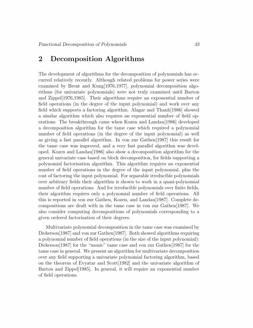
The development of algorithms for the decomposition of polynomials has oc-curred relatively recently. Although related problems for power series wereexamined by Brent and Kung[1976,1977], polynomial decomposition algo-rithms (for univariate polynomials) were not truly examined until Bartonand Zippel[1976,1985]. Their algorithms require an exponential number offield operations (in the degree of the input polynomial) and work over anyfield which supports a factoring algorithm. Alagar and Thanh[1986] showeda similar algorithm which also requires an exponential number of field op-erations. The breakthrough came when Kozen and Landau[1986] developeda decomposition algorithm for the tame case which required a polynomialnumber of field operations (in the degree of the input polynomial) as wellas giving a fast parallel algorithm. In von zur Gathen[1987] this result forthe tame case was improved, and a very fast parallel algorithm was devel-oped. Kozen and Landau[1986] also show a decomposition algorithm for thegeneral univariate case based on block decomposition, for fields supporting apolynomial factorisation algorithm. This algorithm requires an exponentialnumber of field operations in the degree of the input polynomial, plus thecost of factoring the input polynomial. For separable irreducible polynomialsover arbitrary fields their algorithm is shown to work in a quasi-polynomialnumber of field operations. And for irreducible polynomials over finite fields,their algorithm requires only a polynomial number of field operations. Allthis is reported in von zur Gathen, Kozen, and Landau[1987]. Complete de-compositions are dealt with in the tame case in von zur Gathen[1987]. Wealso consider computing decompositions of polynomials corresponding to agiven ordered factorisation of their degrees.
Multivariate polynomial decomposition in the tame case was examined byDickerson[1987] and von zur Gathen[1987]. Both showed algorithms requiringa polynomial number of field operations (in the size of the input polynomial):Dickerson[1987] for the “monic” tame case and von zur Gathen[1987] for thetame case in general. We present an algorithm for multivariate decompositionover any field supporting a univariate polynomial factoring algorithm, basedon the theorem of Evyatar and Scott[1982] and the univariate algorithm ofBarton and Zippel[1985]. In general, it will require an exponential numberof field operations.

34 Mark Giesbrecht
2.1 The Model of Computation
The model of computation used is the “arithmetic Boolean circuit” (see vonzur Gathen [1986]). This model uses inputs x1, x2, . . . , xn from a field F .Operations are the arithmetic (field) operations +, −, ×, /, and Booleanoperations ∧, ∨, and ¬. The connection between the arithmetic and Booleanparts of the circuit is provided by two types of gates. The zero test gategives a Boolean indication of whether or not an input field value is zero. Theselection gate outputs one of two input field values depending upon the valueof a third, Boolean, input. The cost of algorithms will be measured in thenumber of field operations performed. Often, the input will be a polynomialf ∈ F [x] and the number of field operations will be counted in terms of thedegree n of f and the characteristic p of F . If F = GF (pe) for some e ≥ 1,we will also consider the cost of computation over the prime field Zp, andhence in terms of e as well.
Assume we can factor an arbitrary univariate polynomial f ∈ F [x] ofdegree n into irreducible factors in O(SF (n)) field operations. Then we canalso factor a multivariate polynomial g ∈ F [x1, x2, . . . , x`] of total degree
n into irreducible factors. Assume this can be accomplished in O(S(`)F (n))
field operations (where S(`)F (n) is a function of the size (n + 1)` of a dense
representation of the input). Let M(n) be such that the product of twopolynomials of degree at most n can be computed in O(M(n)) field opera-tions. We can choose M(n) = n log n log log n (Schonhage[1977], Cantor andKaltofen[1987]), and M(n) = n log n if F supports a Fast Fourier Transform.Also, assume two n× n matrices can be multiplied in O(nµ) field operationsfor some µ > 2. Coppersmith and Winograd[1987] show µ < 2.38.
In some of our algorithms we use P(S) to denote the set of all subsets(the power set) of a set S, and S∗ to denote the set of finite sequences ofelements of S.
2.2 Computing Right Division
Given f, h ∈ F [x] of degrees n and s respectively with s|n, we would like todetermine if there is a g ∈ K[x] , where K is some algebraic extension of F ,such that f = g h. Lemma 1.1 shows us that if such a g ∈ K[x] exists itwill be in F [x]. We find g by the usual divide and conquer approach, whichis used in von zur Gathen [1987b].
Functional Decomposition of Polynomials 35
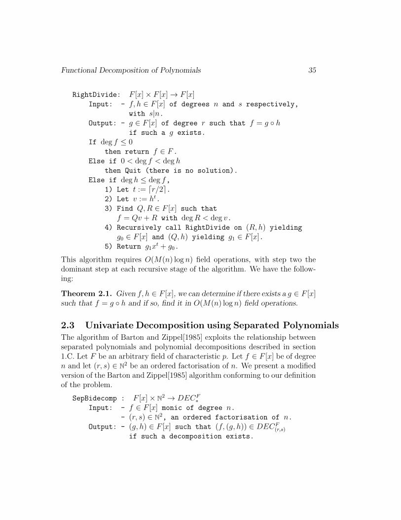
RightDivide: F [x]× F [x]→ F [x]Input: - f, h ∈ F [x] of degrees n and s respectively,
with s|n.Output: - g ∈ F [x] of degree r such that f = g h
if such a g exists.
If deg f ≤ 0then return f ∈ F.
Else if 0 < deg f < deg hthen Quit (there is no solution).
Else if deg h ≤ deg f,1) Let t := dr/2e.2) Let v := ht.3) Find Q,R ∈ F [x] such that
f = Qv +R with degR < deg v.4) Recursively call RightDivide on (R, h) yielding
g0 ∈ F [x] and (Q, h) yielding g1 ∈ F [x].5) Return g1x
t + g0.
This algorithm requires O(M(n) log n) field operations, with step two thedominant step at each recursive stage of the algorithm. We have the follow-ing:
Theorem 2.1. Given f, h ∈ F [x], we can determine if there exists a g ∈ F [x]such that f = g h and if so, find it in O(M(n) log n) field operations.
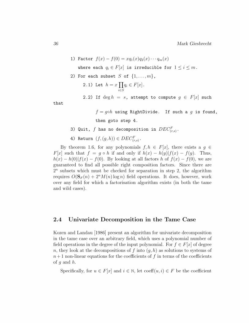
2.3 Univariate Decomposition using Separated PolynomialsThe algorithm of Barton and Zippel[1985] exploits the relationship betweenseparated polynomials and polynomial decompositions described in section1.C. Let F be an arbitrary field of characteristic p. Let f ∈ F [x] be of degreen and let (r, s) ∈ N2 be an ordered factorisation of n. We present a modifiedversion of the Barton and Zippel[1985] algorithm conforming to our definitionof the problem.
SepBidecomp : F [x]× N2 → DECF∗
Input: - f ∈ F [x] monic of degree n.- (r, s) ∈ N2, an ordered factorisation of n.
Output: - (g, h) ∈ F [x] such that (f, (g, h)) ∈ DECF(r,s)
if such a decomposition exists.
36 Mark Giesbrecht
1) Factor f(x)− f(0) = xq1(x)q2(x) · · · qm(x)
where each qi ∈ F [x] is irreducible for 1 ≤ i ≤ m.
2) For each subset S of 1, . . . ,m,
2.1) Let h = x∏i∈Sqi ∈ F [x].
2.2) If deg h = s, attempt to compute g ∈ F [x] such
that
f = gh using RightDivide. If such a g is found,
then goto step 4.
3) Quit, f has no decomposition in DECF(r,s).
4) Return (f, (g, h)) ∈ DECF(r,s).
By theorem 1.6, for any polynomials f, h ∈ F [x], there exists a g ∈F [x] such that f = g h if and only if h(x) − h(y)|f(x) − f(y). Thus,h(x) − h(0)|f(x) − f(0). By looking at all factors h of f(x) − f(0), we areguaranteed to find all possible right composition factors. Since there are2n subsets which must be checked for separation in step 2, the algorithmrequires O(SF (n) + 2nM(n) log n) field operations. It does, however, workover any field for which a factorisation algorithm exists (in both the tameand wild cases).
2.4 Univariate Decomposition in the Tame Case
Kozen and Landau [1986] present an algorithm for univariate decompositionin the tame case over an arbitrary field, which uses a polynomial number offield operations in the degree of the input polynomial. For f ∈ F [x] of degreen, they look at the decompositions of f into (g, h) as solutions to systems ofn+ 1 non-linear equations for the coefficients of f in terms of the coefficientsof g and h.
Specifically, for u ∈ F [x] and i ∈ N, let coeff(u, i) ∈ F be the coefficient

Functional Decomposition of Polynomials 37
of xi in u. Let
f =∑
0≤i≤naix
i ∈ F [x] with ai ∈ F for 0 ≤ i ≤ n,
g =∑
0≤i≤rbix
i ∈ F [x] with bi ∈ F for 0 ≤ i ≤ r,
h =∑
1≤i≤scix
i ∈ F [x] with ci ∈ F for 1 ≤ i ≤ s,
µk =∑
s−k+1≤i≤scix
i ∈ F [x] with ci ∈ F for s− k + 1 ≤ i ≤ s and 1 ≤ k ≤ s.
If f = g h, the following facts are easily seen to be true:
(i) coeff(hr, n− e)= coeff(f, n− e) = an−e for 0 < e < s,(ii) coeff(hr, n− e)= coeff(µrk, n− e) for e < k ≤ s.
This implies an−e = coeff(f, n − e) = coeff(µrk, n − e) for e < k ≤ s. For1 ≤ k < s, we know µk+1 = µk + cs−kx
s−k. By binomial expansion we get
µrk+1 = (µk + cs−kxs−k)r
= µrk + rcs−kxs−kµr−1
k + ϕ,
where ϕ ∈ F [x] and degϕ ≤ rs − 2k. Thus coeff(µrk+1, rs − k) = ars−k =coeff(µrk, rs− k) + rcs−k. This gives the simple recurrence
cs−k =ars−k − coeff(µrk, rs− k)
r,
which allows the computation of cs, cs−1, . . . , c1 in turn, and hence the calcu-lation of h. Note that it is at this point, and only this point, that we requirethat p - r. This distinguishes the tame and wild cases.
This system of equations uniquely determines an h ∈ F [x] but a g ∈ F [x]such that f = g h may or may not exist. We can determine the existenceof such a g, and if it exists, find it, using RightDivide as described earlier.Kozen and Landau[1986] show that a decomposition can be computed inO(n3) field operations in general and O(n2 log n) field operations in a fieldwhich supports a Fast Fourier Transform. In fact, the algorithm works overany ring in which r is a unit.
In von zur Gathen[1987], an improvement of the result of Kozen andLandau[1986] is shown. Given a monic f ∈ F [x] of degree n and (r, s) an

38 Mark Giesbrecht
ordered factorisation of n with p - r, his algorithm determines if there existsa decomposition of f in DECF
(r,s) and, if so, finds it, in O(M(n) log n) fieldoperations. The number of field operations required is dominated by the costof RightDivide to obtain g from f and h. Von zur Gathen[1987] uses thisalgorithm for decomposition to obtain the set of separated factors of a givenpolynomial f ∈ F [x] of degree n in polynomial time in the tame case.
A very fast parallel algorithm is also presented by von zur Gathen[1987]for univariate bidecomposition in the tame case. He shows that over any fieldF , given f ∈ F [x] and (r, s), an ordered factorisation of n such that p - r,it can be determined if there exists a decomposition of f in DECF
(r,s), and ifso, it can be found, with a depth O(log n) circuit over F .
2.5 Decomposition using Block Decomposition
As seen in section 1.D, the polynomial decomposition problem can be refor-mulated as one of finding functional block decompositions. Let f ∈ F [x] bemonic of degree n, and (r, s) an ordered factorisation of n. Kozen and Lan-dau[1987] adapt the techniques from Landau and Miller[1983] to constructall block decompositions of dimension two of f in BLOCKSF(r,s). They thencheck each such decomposition to see if it is functional. In general, however,their algorithm requires a number of field operations exponential in n. Iff is separable and irreducible over F , they show that there can be at mostnlogn block decompositions in BLOCKSF(r,s), and that each block decomposi-tion can be constructed in a polynomial number of field operations. Testinga block decomposition to see if it is functional requires only a polynomialnumber of field operations, but we may have to check all of them. Therefore,for separable irreducible polynomials f ∈ F [x], it can be determined if f hasa decomposition in DECF
(r,s), and if so, this decomposition can be found, in
a quasi-polynomial number (nO(logn)) of field operations over F .The block decompositions of irreducible polynomials over a finite field
F = GF (q) (where q = pe for some e ≥ 1) have a stronger structure. Letf ∈ F [x] of degree n be irreducible with splitting field K = F [x]/(f), andlet (r, s) be an ordered factorisation of n. The roots of f in K have theform α, αq, αq2 , . . . , αqn−1 for any one root α ∈ K of f . The Galois groupof K relative to F is the set of automorphisms σi : 0 ≤ i < r withσiγ = γq
ifor any γ ∈ K. Kozen and Landau[1986] note that the only
possible block decomposition of f has the form B = Ci|0 ≤ i < r where

Functional Decomposition of Polynomials 39
Ci = αqi+jr |0 ≤ j < s for 0 ≤ i < r. It is functional (and hence correspondsto a polynomial decomposition) if and only if there exists an h ∈ F [x] suchthat for 0 ≤ i < r, there exists a γi ∈ K such that∏
0≤j<s(x− αqi+jr) = h− γi.
The splitting field K of f is an algebraic extension of degree n over F , so wecan easily compute a representation of these roots (in K), and check if thisblock decomposition is functional in a polynomial number of field operations.Kozen and Landau[1986] show that in this case, it can be determined if apolynomial f has a bidecomposition inDECF
(r,s), and if so, this decomposition
can be found, with a circuit of depth O(log epn log2 n) and size (epn)O(1). Weshow the sequential analysis of this algorithm in the following theorem.
Theorem 2.2. Let F = GF (q) for some q, p, e ∈ N with p prime and q = pe,and let f ∈ F [x] be irreducible of degree n. If (r, s) is an ordered factorisationof n we can determine if there exists a decomposition of f in DECF
(r,s), and
if so, find it, in O(n2M(n) log q) field operations over F .
Proof. Let K = F [z]/(f) and let α ≡ z mod f ∈ K. Multiplication in Krequires O(M(n)) field operations in F . We can therefore compute αq
rifor
all i with 0 ≤ i < s with ∑0≤i<s
ri log q = O(rs2 log q)
= O(n2 log q)
field operations over K or O(n2M(n) log q) field operations over F . We thencheck if
∏0≤i<s(x−αq
ri) = h+c where h ∈ F [x] and c ∈ K. If so, there exists
a g such that (f, (g, h)) ∈ DECF(r,s) and this can be found in O(M(n) log n)
field operations by theorem 2.1. We can compute∏
0≤i<s(x− αqri
) in O(n2)field operation over K or O(n2M(n)) field operation over F . Therefore thebidecomposition problem can be solved sequentially for irreducible polyno-mials over finite fields with O(n2M(n) log q) field operations over F .
2.6 A Lower Bound on the Degrees of Splitting FieldsLet F be a field such that for any m ∈ N, there exists an algebraic extension ofF of degree m over F . We will now show that in any such field, for any n ∈ N,

40 Mark Giesbrecht
there exist polynomials of degree n over F with splitting fields of degreeexponential in n over F . Note in particular that finite fields are included inthis theorem. One implication of this is that we cannot construct a standardrepresentation of elements of such a splitting field in a polynomial number offield operations. It has been known for a long time that over the rationals andsome other infinite fields that for any n, there exist polynomials of degreen whose Galois groups are Sn. The splitting fields of these polynomialsare of algebraic degree n! over their ground fields. In general however, suchpolynomials do not exist (see van der Waerden section 8.10, Jacobson section4.10). We instead make the following construction in an arbitrary field F .Let pi ∈ N be the ith smallest rational prime. Also define
ϑ(`) =∑
p primep≤`
log p the Chebyshev ϑ function,
π(`) =∑
p primep≤`
1
(where all logarithms here and throughout this section are natural). Letfi ∈ F [x] be an irreducible polynomial of degree pi. The splitting field Ki
of fi has degree at least pi over F . If F is a finite field, [Ki : F ] = pi.The polynomial hi = f1f2 . . . fi will have splitting field Li generated by theelements of K1 ∪ K2 ∪ · · · ∪ Ki. This is a field of algebraic degree at leastp1p2 . . . pi over F . Let
S(`) =∑
p primep≤`
p,
R(`) =∏
p primep≤`
p.
Note that R(`) = exp(ϑ(`)).
Let n ∈ N. If k = maxi| pi ≤ `, then hk has a splitting field of degreeR(`) over F . We will show that if ` ≤ 0.77
√n log n, then deg hk = S(`) ≤
n. It follows that R(0.77√n log n) is exponential in n. If f ∈ F [x] is any
polynomial of degree n with divisor hk, we show that f has a splitting fieldof degree at least exp(0.5
√n log n) over F . We will use the following bounds
from Rosser and Schoenfeld[1962]:

Functional Decomposition of Polynomials 41
Fact 2.3.
(i) pk < 1.4k log k for k ≥ 6;
(ii) π(`) ≤ 1.26`/ log ` for ` ≥ 17;
(iii) `(1− 1/ log `) < ϑ(`) for n ≥ 41.
First, we show an upper bound on the function σ(k) = S(pk) =∑
1≤i≤k pi,the sum of the first k primes, for k ∈ N.
Lemma 2.4. For k ≥ 6, σ(k) ≤ 0.86k2 log k
Proof.
σ(k) ≤ 2 + 3 + 5 + 7 + 11 + 1.4∑
6≤i≤ki log i
≤ 28 + 1.4∫ k
6(i+ 1) log(i+ 1)di
≤ 28 + 1.4(0.5(i+ 1)2 log(i+ 1)− 0.25(i+ 1)2∣∣∣k6)
≤ 0.86k2 log k
Lemma 2.5. For any n ≥ 109, S(0.77√n log n) ≤ n.
Proof. Applying lemma 2.4 to the the upper bound on the number of primesless than ` provided by fact 2.3(ii),
S(`) ≤ 0.86
(1.26`
log `
)2
log
(1.26`
log `
)
≤ 0.86(1.26)2 `2
(log `)2(log(1.26`)− log log `)
≤ 1.37`2
(log `)2(log `+ log 1.26− log log `)
≤ 1.7`2
log `
for ` ≥ 17. For n ≥ 109 this gives us
S(0.77√n log n) ≤ 1.7(0.77
√n log n)2
log(0.77√n log n)
≤ n
log(0.77√n log n)
≤ n,
and the lemma follows.

42 Mark Giesbrecht
Theorem 2.6. For n ≥ 109 there exists a polynomial f ∈ F [x] of de-gree n such that the splitting field of f has degree over F greater thanexp(0.5
√n log n).
Proof. By lemma 2.5, if ` ≤ 0.77√n log n, then S(`) ≤ n. Let ` =
b0.77√n log nc. Let k = maxi| pi ≤ `. The polynomial hk has a split-
ting field Lk with degree at least R(`). By definition
R(`) = exp(ϑ(`))
≥ exp(`(1− 1/ log `))
≥ exp(0.77√n log n(1− 1/ log(0.77
√n log n)))
≥ exp(0.5√n log n),
for n ≥ 109. Therefore hk has a splitting field of degree at least exp(0.5√n log n).
Let f be any polynomial of degree n such that hk divides f (hk has de-gree less than n). The polynomial f has a splitting field of degree at leastexp(0.5
√n log n) over F .
2.7 Decompositions Corresponding To Ordered FactorisationsLet f ∈ F [x] be of degree n and let ℘ = (rm, rm−1, . . . , r1) be an orderedfactorisation of n. A natural generalisation of the computational bidecompo-sition problem is to compute the decompositions of f in DECF
℘ (if any). LetGenericBidecomp be an algorithm such that given f ∈ F [x] of degree n, and(r, s) ∈ N2, an ordered factorisation of n, it will find the (possibly empty) setB of decompositions of f in DECF
(r,s) using D(n) field operations. Considerthe following algorithm:
OrdFactDecomp: F [x]×P(N)→ P(DECF∗ )
Input: - f ∈ F [x] of degree n,- ℘ = (rm, rm−1, . . . , r1), an ordered factorisation of n.
Output: - the set of decompositions of f in DECF℘ .
If m = 1then return (f, (f))else
1) Find the set B of bidecompositions
(f, (g, h)) ∈ DECF(t2,r1)

Functional Decomposition of Polynomials 43
where t2 =∏
2≤i≤m ri,using GenericBidecomp.
2) Let T := ∅.3) For each decomposition (f, (g, h)) ∈ B,
3.1) Recursively attempt to
find a decomposition
(g, (gm, gm−1, . . . , g2)) ∈ DECF(rm,rm−1,...,r2).
3.2) If such a decomposition of g is found
add (f, (gm, gm−1, . . . , g2, h)) to T.4) Return T.
This is simply a recursive application of the bidecomposition algorithm,and can easily be seen to return the set of decompositions of f in DECF
℘ .We now define a ℘-easy family of polynomials, a family in which such de-
compositions can be computed quickly. For 1 ≤ i ≤ m, let ℘i = (rm, rm−1, . . . , ri)and ti =
∏i≤j≤m rj. A set F℘ ⊆ F [x] is ℘-easy if
(i) for any i with 1 ≤ i < m, any f ∈ F℘ of degree d has at most onedecomposition in DECF
(ti+1,ri),
(ii) it can be determined if such a decomposition exists, and if it does, itcan be found with O(D(d)) = dO(1) field operations, and
(iii) if f ∈ F℘ and (f, (g, h)) ∈ DECF(ti+1,ri)
then g ∈ F℘.
If F℘ ⊆ F [x] is a ℘-easy family of polynomials, then the bidecompositionsof f ∈ F℘ in step 1 can be found in D(n) field operations. Thus, com-puting OrdFactDecomp on f ∈ F℘ with ordered factorisation ℘ requiresO(∑
1≤i<mD(ti)) field operations. Let ` = dlog2 ne and let κ = (e`, e`−1, . . . , e1),where ei = 2i for 1 ≤ i ≤ `. Noting that n ≤ ` < 2n, it follows immediatelythat e`−j ≥ fm−j for 0 ≤ j < m. Therefore
∑1≤i<mD(ti) ≤
∑1≤i<`D(ei).
Since D is polynomially bounded,∑
1≤i<`D(ei) = O(D(n)). We have shownthe following theorem:
Theorem 2.7. Let n ∈ N and let ℘ be an ordered factorisation of n. Also,let F℘ ⊆ F [x] be ℘-easy. Then, for any f ∈ F℘, we can determine if thereexists a decomposition of f in DECF
℘ , and if so, find it, in O(D(n)) fieldoperations.

44 Mark Giesbrecht
This theorem says that the general problem of computing the set of de-compositions of a polynomial with a given ordered factorisation is Cook re-ducible to the bidecomposition problem for ℘-easy families of polynomials.
Two ℘-easy families present themselves immediately. If F is an arbitraryfield and p - ri for 1 < i ≤ m then F [x] is a ℘-easy family of polynomials. Thisfollows because all the bidecompositions performed in step 1 are tame. Fromvon zur Gathen[1987] and theorem 2.7 above, it can be determined whethera decomposition of f ∈ F [x] exists in DECF
℘ and if so such a decompositioncan be found in O(M(n) log n) field operations.
If F = GF (q) and F℘ is the set of polynomials irreducible over F , thenF℘ is ℘-easy. This follows since, if f ∈ F℘ and (f, (g, h)) ∈ DECF
∗ , then gis also irreducible over F . By theorem 2.2 and theorem 2.7, a decompositionof any f ∈ F℘ can be found in O(n2M(n) log q) field operations.
2.8 Computing Complete Univariate Decompositions
The following method for computing complete decompositions was suggestedin von zur Gathen[1987] for the tame case and can be applied whenever wecan do bidecomposition. Let D(n) be the number of field operations requiredto find a bidecomposition of f ∈ F [x] corresponding to an ordered factorisa-tion (r, s) of n. The following algorithm computes a complete decompositionof f in DECF
∗ .
CompleteDecomposition: PF → cDECF∗
Input: - f ∈ F [x].Output: - (f, (fm, fm−1, . . . , f1)) ∈ cDECF
∗ .
1) Compute the integer factorisation n = pe11 pe22 · · · pekk of n.
2) Let d(n) = (e1 + 1) · · · (ek + 1) be the number of divisors
of n and 1 = r1 < r2 < · · · < rd(n) = n be the divisors of n.3) Let j > 1 be the smallest number such that f has a
decomposition (f, (g, h)) ∈ DECF(rj ,n/rj)
.
4) If j = d(n) then f is indecomposable; otherwise
decompose h recursively (g is indecomposable
since any left composition factor of g is a
composition factor of f of smaller degree than g).
The number of field operations required by this algorithm is O(D(n)d(n)).Hardy and Wright[1960] (theorem 317) show that d(n) = O(nε) for all ε >
Functional Decomposition of Polynomials 45
0. Therefore, we can compute complete decompositions in O(D(n)nε) fieldoperations for any ε > 0. This algorithm finds the lexicographically firstcomplete decomposition of f .
2.9 Decomposing Multivariate Polynomials in the TameCase
Once again we denote the sequence of indeterminates x1, . . . , x` as ~x. Wedefine the set W(`)
F ⊆ F [~x] of monic polynomials in F [~x] as follows:
W(`)F =
f = xd11 xd22 · · ·x
d`` + f
∣∣∣∣ f ∈ F [~x], deg f < deg f
di ∈ N \ 0, degxi f ≤ di for 1 ≤ i ≤ `
where deg f and deg f are the total degrees of f and f respectively. Dick-erson[1987] uses much the same method as Kozen and Landau[1986] did forthe univariate case to decompose monic multivariate polynomials in the tamecase. Given a monic f ∈ F [~x] of degree n and r ∈ N, he shows how to finda monic g ∈ F [x] of degree r and monic h ∈ F [~x] of degree r = n/s suchthat f = g h. The computation requires O(n3`) field operations. From thealgorithm it is seen that if such a decomposition exists, it is unique. Notethat monic multivariate polynomials are a very special case of multivariatepolynomials. Just because they can be decomposed does not mean that mul-tivariate polynomials can be decomposed in the tame case in general (thoughit is possible a reduction from the general case exists).
In von zur Gathen[1987], the tame case for the decomposition of mul-tivariate polynomials is dealt with completely. He first defines the set ofpolynomials P(`)
F ⊆ F [~x] which are strongly monic in x1 as follows:
P(`)F =
f =∑
0≤i≤nfix
i1 ∈ F [~x]
∣∣∣∣ n ∈ N, f0, . . . , fn ∈ F [x2, . . . , x`]
fn = 1, deg f = n
.If f ∈ F [~x] is strongly monic and f = g h, then f(x1, 0, . . . , 0) = g h(x1, 0, . . . , 0). As we know f(x1, 0, . . . , 0) is of degree n (f is strongly monic),the univariate decomposition of f(x1, 0, . . . , 0) in DECF
(r,s) completely deter-mines g ∈ F [x] in the multivariate decomposition. Once g is computed, alinearly convergent Newton iteration is used to compute h ∈ F [~x] in a num-ber of field operations polynomial in the input size. Given f ∈ F [~x] and

46 Mark Giesbrecht
g ∈ F [x], the process of finding h ∈ F [~x] such that f = g h is a specialcase of (multivariate) power series reversion. This is dealt with extensivelyby Brent and Kung[1977,1978]. They show the problem is linearly equivalentto power series composition when (∂g/∂x) 6= 0, which is true in the tamecase. Furthermore, they show that multivariate polynomial reversion can becomputed in O((n log n)
12M(n)`) field operations.
For an arbitrary f ∈ F [~x] we can use substitutions of the form σ(xi) =xi + σix1 with xi ∈ F for 2 ≤ i ≤ m to make f strongly monic. For sucha substitution σ we write σf = f(x1, x2 + σ2x1, . . . , xm + σmx1). This sub-stitution σ may be inverted by the substitution σ−1 = (−σ2,−σ3, . . . ,−σm)and σσ−1f = f . For a suitably chosen substitution σ, f = aσf is stronglymonic in x1 (where a ∈ F is chosen to make the highest order coefficient ofx1 in aσf one). If f = g h for g, h ∈ F [x] then f = (a−1g) (σ−1h) is acorresponding decomposition of f .
For f ∈ F [~x] of total degree n, von zur Gathen[1987] shows how tochoose a substitution σ such that σf is strongly monic. This can be done ina polynomial number of field operations in m,n, and k, where k is the numberof monomials in f . (the sparse representation of f has size O(km log n)). For0 ≤ i ≤ n, let ui ∈ F [x2, . . . , xm] be the homogenous part of degree n− i ofthe coefficient of xi1 in f . The homogenous part of degree n of f is therefore∑
0≤i≤n uixi 6= 0, and by the homogeneity of the ui’s, u =
∑0≤i≤n ui is also
nonzero, and of degree at most n. Let K be an extension field of F withmore than n points. K can be chosen as a field of degree O(log n) over F .Now, for a substitution σ = (σ2, σ3, . . . , σm), degx1 σf = n if and only if
deg f(x1, σ2x1, . . . , σmx1) = deg[(σ)(x1, 0, . . . , 0)] = n.
This is true if and only if u(σ2, σ3, . . . , σm) 6= 0. To find σ2, . . . , σm we proceedin stages i from 2 to m. At stage i we choose σi ∈ K such that
u(σ2, . . . , σi, xi+1, . . . , xm)
is nonzero. We do this by considering vi = u(σ2, . . . , σi−1, xi, . . . , xm) as apolynomial in K(xi+1, . . . , xm)[xi] of degree in xi at most n. Thus vi has atmost n roots in K(xi+1, . . . , xm) and we can find a non-root σi ∈ K of viwith at most n evaluations of vi at points in K. Assume f is the sum of atmost k monomials. Then u is also the sum of at most k monomials and σ canbe found in O(kmn log n) field operations over K or O(kmn log nM(log n))

Functional Decomposition of Polynomials 47
field operations over F . Decomposing multivariate polynomials is, therefore,polynomial time (in the input degree and the size of the sparse representation)reducible to decomposing strongly monic multivariate polynomials.
2.10 Multivariate Decomposition Using Separated Polynomials
Using theorem 1.15 we can generalise the algorithm of Barton and Zip-pel[1985] to the multivariate case and obtain a multivariate decompositionalgorithm for any field supporting a factorisation algorithm. To do this wemust show a “right division” algorithm for the multivariate case. Namely,given f, h ∈ F [~x], we must be able to find a g ∈ F [x] such that f = g h (ifsuch a g exists). We cannot use the “Taylor Expansion” method of the uni-variate case directly. Instead we use the methods of von zur Gathen[1987] totransform the problem to one involving strongly monic polynomials. Anothersimple transformation yields a univariate problem such that the solution isthe same as in the original problem.
MultiRightDivide: F [~x]× F [~x]→ F [x]Input: - f, h ∈ F [~x] of total degrees n and s respectively.
Output: - g ∈ F [x] of degree r = n/s such that f = g h(if such a g exists).
1) Let K be an algebraic extension of F with
more than n elements.
Let σ = (σ2, σ3, . . . , σm) ∈ Km−1
be a substitution and a ∈ K such that
f = aσf = f(x1, x2 + σ2x1, . . . , xm + σmx1) ∈ K[x]is strongly monic (see previous section).
2) Let h = σh.3) Using RightDivide determine if there exists a g ∈ K[x]
such that f(x, 0, . . . , 0) = g h(x, 0, . . . , 0)and if so find it. If no such g exists, quit.
4) Return g = a−1g.
In the previous section we saw that step 1 can be performed inO(kmn log nM(log n)) field operations over F , where k is the number ofmonomials in f . It follows that f = g h if and only if aσf = ag σh. Sinceaσf is strongly monic, there exists a g ∈ F [x] such that aσf = ag σh if andonly if aσf(x, 0, . . . , 0) = ag σh(x, 0, . . . , 0). Using RightDivide we can

48 Mark Giesbrecht
determine the existence of g = ag, and if it exists find it, in O(M(n) log n)field operations over K or O(M(n) log nM(log n)) field operations over F . Ifg exists we can immediately compute g, and the whole computation requiresO((kmn log n+M(n) log n)M(log n)) field operations over F
The algorithm for multivariate decomposition over any field supportinga factorisation algorithm proceeds in much the same way as the Barton andZippel[1985] algorithm for the univariate case.
MultiSepDecomp : F [~x]× N2 →MDECF∗
Input: - f ∈ F [~x] of degree n- (r, s) ∈ N2, an ordered factorisation of n
Output: - (g, h) ∈ (F [x]× F [~x]) such that f = g hif such a decomposition exists
1) Factor f(~x)− f(0, . . . , 0) = ~xq1(~x)q2(~x) · · · qm(~x)where each qi ∈ F [~x] is irreducible for 1 ≤ i ≤ m
2) For each subset S of 1, . . . ,m2.1) Let h = ~x
∏i∈Sqi ∈ F [~x].
2.2) If deg h = s, attempt to compute g ∈ F [x] such
that
f = g h using MultiRightDivide.
If such a g is found, then goto step 4.
3) Quit, f has no decomposition in MDECF(r,s).
4) Return (f, (g, h)) ∈MDECF(r,s).
The number of subsets of S is 2n. This algorithm can, therefore, be com-pleted with O(SF (n) + 2n(kmn log n+M(n) log n)M(log n)) field operationsover F . It does, however, work in both the tame and wild cases over anyfield supporting a polynomial factorisation algorithm.

Functional Decomposition of Polynomials 49
3 Additive Polynomials3.1 Definition and Root Structure of Additive PolynomialsLet F be an arbitrary field of characteristic p greater than zero. Define apolynomial f ∈ F [x] to be an additive polynomial if, for independent inde-terminates x and y,
f(x+ y) = f(x) + f(y).
The non-zero additive polynomials in F [x] are exactly those of the form
f =∑
0≤i≤νaix
pi
where ν ∈ N, ai ∈ F for 1 ≤ i ≤ ν, and aν 6= 0. The integer ν is called theexponent of f , and we write “expn f = ν”. We denote the set of additivepolynomials over F as AF.
The additive polynomials have a well understood decomposition struc-ture which leads to a number of interesting results on decomposition in thegeneral case. This structure was first developed in Ore[1933b], who inves-tigated the vector space structure of the roots of additive polynomials (aswell as investigating the ring structure of the additive polynomials undercomposition – see chapter 4). This work was continued by Whaples[1954],who examined the Galois groups of additive polynomials and characterisedadditive polynomials in terms of these groups. In Dorey and Whaples, theGalois group Gf of Φf = f − f(x) ∈ F (f)[y] (where f ∈ AF) is used (see sec-tion 1.B) to show that all normal decompositions of additive polynomials aredecompositions into additive polynomials. We use this approach to developmuch of the structure of the roots of additive polynomials in terms of Gf .Though the theorems in this section are for the most part known (with thepossible exception of theorem 3.2(i)), the extension of the approach of Doreyand Whaples is of interest. For a given additive polynomial f ∈ AF, it servesto illustrate the strong connection between the separated factors of Φf , theGalois structure of f (which is the basis for block decompositions), and theGalois structure of Φf . Not coincidentally, each of these three approachesleads to at least one algorithm – the first being the separated polynomialalgorithms of Barton and Zippel and Alagar and Thanh, the second beingthe block decomposition algorithm of Kozen and Landau, and the last be-ing a number of algorithms specifically for additive polynomials, which arepresented in chapter 5.

50 Mark Giesbrecht
Theorem 3.1.
(i) Let f ∈ AF be monic, with exponent ν such that f is squarefree (a0 =f ′(0) 6= 0). Let K be the splitting field of f . Then the roots of f in Kform a vector space Vf over Zp of dimension ν.
(ii) For each finite Zp-vector space V ⊆ F of dimension ν, there exists aunique monic f ∈ AF with exponent ν such that the roots of f areexactly the elements of V .
Proof.
(i) For α, β ∈ K such that f(α) = f(β) = 0, we see that
f(α + β) = f(α) + f(β) = 0,
f(kα) = kf(α) = 0 for any k ∈ Zp.
Since f ′(0) 6= 0, the greatest common divisor of f and f ′ is one, andhence f has no multiple roots. Therefore Vf has pν distinct elementsand dimension ν.
(ii) Let (θ1, . . . , θν) be a basis for V in F over Zp. The polynomial
Ψ1 = xp − θp−11 x ∈ AF
has roots kθ1 for all k ∈ Zp. For i ≥ 2, define
Ψi = (xp −Ψi−1(θi)p−1x) Ψi−1 ∈ AF.
If Ψi−1(α) = 0 for α ∈ F then Ψi(α) = 0. Also,
Ψi(θi) = Ψi−1(θi)p −Ψi−1(θi)
p−1Ψi−1(θi) = 0.
Since Ψi is additive, Ψi has roots consisting of all Zp-linear combinationsof θ1, . . . , θi. Thus the roots of Ψi are exactly the members of thevector space with basis (θ1, . . . , θi). Let f = Ψn, which is monic andadditive. This f is also unique by virtue of being a monic interpolantof degree pν of pν distinct points. Note also that f ′(0) 6= 0 as f has pν
distinct roots in f and degree pν .
Functional Decomposition of Polynomials 51
Call the Zp-vector space V of roots of an additive polynomial f ∈ F [x] thekernel of f . Say an additive polynomial is simple if it is monic and f ′(0) 6= 0.In this section we will deal almost exclusively with simple additive polyno-mials. Non-simple monic additive polynomials are just simple polynomialscomposed on the right with xp
`for some ` > 0. Assume f ∈ AF is monic and
f = g xp` ∈ AF where g ∈ AF is simple and
g =∑
0≤i≤σbix
pi
with σ ∈ N, bi ∈ F , and bσ 6= 0. Then
f =∑
0≤i≤σbix
pi+`
= xp`
∑0≤i≤σ
(bi)1
p` xpi
= xp` g
whereg =
∑0≤i≤σ
(bi)1
p` xpi ∈ AK
and K is an algebraic extension of F . So f has a kernel of dimension σ,namely the kernel of g. If F is perfect (and hence closed under pth roots) gwill be in F [x] as well.
Let f ∈ AF be simple with exponent ν, splitting field K and kernel Vf ⊆K. The structure of the kernel of f and that of the fields between K(f) andK(x) (and hence the structure of the decompositions of f over its splittingfield) are closely linked. Let Φf = f(y) − f ∈ F (f)[y] ⊆ F (x)[y] withsplitting field Ω ⊇ F (f) and Galois group Gf = Gal(Ω/F (f)) as in theorem1.5. Because ∂
∂yΦf = ∂
∂yf(y) 6= 0, Ω is a separable field extension of F (f).
Theorem 3.2.
(i) K(x) is the splitting field of Φf ,
(ii) Gf is the group x 7→ x+α | α ∈ K, f(α) = 0 under composition, and
(iii) Vf ∼= Gf .
52 Mark Giesbrecht
Proof.
(i) For α ∈ Vf ,Φf (x+ α) = f(x+ α)− f(x)
= f(x) + f(α)− f(x)
= 0.
Since Φf has degree pν over F (f), x + Vf is the complete set of rootsof Φf . We know that x ∈ x+ Vf and K is the smallest extension fieldof F containing Vf , so Ω = K(x).
(ii) From (i), all roots of Φf are of the form x + α where α is a root of fin K. Therefore, Gf contains the pν automorphisms x 7→ x + α | α ∈K , f(α) = 0. Since [F (x) : F (f)] = pν , this is the entire Galoisgroup.
(iii) From (ii), Gf is isomorphic to a set of monic linear elements in K[x]under composition. Trivially this is isomorphic to the group of constantterms of these elements under addition. These constant terms are allthe roots of f in K, so Gf ∼= Vf .
Theorem 3.3. Let f ∈ AF be simple of exponent ν. Let g, h ∈ F [x] be ofdegrees r = pρ and s = pσ respectively such that (f, (g, h)) ∈ DECF
(r,s). Then
(i) g and h are additive and simple, and
(ii) h has kernel Vh ∼= Gh, where Gh ⊆ Gf is the subgroup fixing F (h) ⊆F (x) pointwise.
Proof. By theorem 1.5, the automorphisms in Gf fixing F (h) form a groupGh such that Gx ⊆ Gh ⊆ Gf , and the index of Gx in Gh is pσ. From theorem3.2(i), K(x) is the splitting field of Φf , so Gx is the identity group, and thecardinality of Gh is pσ. From the isomorphism between Gf and Vf , thereis a subspace W of Vf of dimension σ corresponding to the subgroup Gh.Let h ∈ K[x] be the simple additive polynomial with kernel W . For allα ∈ W , h(x + α) = h(x) + h(α) = h(x). Thus F (h) is fixed by Gh. Bytheorem 3.1, h is unique, so h = h. Now, for algebraically independentindeterminates x and y, f = g(h(x + y)) = g(h(x) + h(y)) and since f is

Functional Decomposition of Polynomials 53
additive f = g(h(x)) + g(h(y)). Thus g is monic and additive. If g is notsimple then g = g xp` for some simple additive polynomial g ∈ K[x] and` > 0. But then f = g xp` h = g hpl which is not simple. So g is simpleas well.
3.2 Rationality and the KernelIf f ∈ AF is simple with kernel Vf ⊆ K and splitting field K, a subspaceVh ⊆ Vf is said to be rational if the simple polynomial h ∈ AK correspondingto Vh is in AF. We would also like to formulate rationality in terms of thestructure of the kernel.
Theorem 3.4. A subspace Vh of Vf is rational if and only if Vh is invariant(as a set) under Gf = Gal(K/F ).
Proof. Assume h ∈ AF. The coefficients of h are the values of the elementarysymmetric functions of the roots of h in K. The automorphisms in Gf leavethese coefficients fixed, and must therefore leave Vh invariant (as a set).
Conversely, if Vh is invariant under Gf then the values of the elementarysymmetric functions of the elements of Vh are fixed under Gf , and so are inF . These are exactly the coefficients of h and so h ∈ AF.
When dealing with a finite field F a somewhat stronger structure can beshown.
Theorem 3.5. Let F = GF (q) where q = pe ∈ N for some p, e ∈ N with pprime. Let K be an algebraic extension of F and f ∈ AK of exponent ν withkernel Vf and splitting field L. Then f ∈ AF if and only if V q
f = Vf .
Proof. If f ∈ AF and α is a root of f in L, then so is αq. This followssince, if g ∈ F [x] is the minimal polynomial of α, g|f and g(αq) = 0 (α andαq are conjugates since F is finite). Thus V q
f ⊆ Vf . Since x → xq is anautomorphism of L over F , V q
f = Vf .If V q
f = Vf then we must show that f ∈ F [x]. The group H of automor-phisms of L over F is the group generated by the automorphism x → xq.Thus Vf is invariant (as a set) under H. As the coefficients of f are symmet-ric functions of the elements of Vf , they are fixed by H, and therefore mustbe in F . Hence f ∈ AF.
The preceding theorem gives the following alternative formulation of thebidecomposition problem for additive polynomials:

54 Mark Giesbrecht
Let F = GF (q) where q, p, e ∈ N, p is prime, and q = pe. Let K bean algebraic extension of F and let V ⊆ K be a Zp vector space ofdimension ν over Zp such that V q = V . For a given σ with 1 ≤ σ ≤ ν,determine if there exists a σ dimensional subspace W of V such thatW q = W , and if so, give a basis for some predetermined number ofthem.
Since V q = V , all the elements of V can be specified as the roots of asingle additive polynomial f ∈ AF of exponent ν. The found subspace W(if it exists) will be the kernel of a right composition factor h ∈ AF of f ofexponent σ.
3.3 Rational Decompositions of Additive PolynomialsWe can now talk about decompositions of simple additive polynomials ingeneral and their relationship to their kernels. For any n,m ∈ N, let
℘ = (rm, rm−1, . . . , r1)
= (pρm , pρm−1 , . . . , pρ1)
be an ordered factorisation of n. Define
APDECF℘ =
(f, (fm, . . . , f1)) ∈ AF × (AF)
m∣∣∣ f = fm · · · f1
and deg fi = ri = pρi
.
Similarly, for simple additive polynomials, define
SAPDECF℘ =
(f, (fm, . . . , f1)) ∈ AF × (AF)
m
∣∣∣∣∣ f simple, f = fm · · · f1,
and deg fi = ri = pρi
.
Obviously SAPDECF℘ ⊆ APDECF
℘ ⊆ DECF℘ .
Let di =∏
1≤j≤i
rj and V be the set of all finite Zp -vector spaces in F . Define
FLAGSF℘ =
(f, (Vm, . . . , V1)) ∈ AF × Vm∣∣∣∣∣f simple, Vm is the kernel of f,
Vm ⊇ Vm−1 ⊇ · · · ⊇ V1,
dimVi = di, for 1 ≤ i ≤ m
.The sequence Vm ⊇ Vm−1 ⊇ · · · ⊇ V1 is called a flag of vector spaces associ-ated with f .
Functional Decomposition of Polynomials 55
Let f ∈ AF be simple. For any (f, (fm, . . . , f1)) ∈ SAPDECF℘ let hi =
fi fi−1 · · · f1 ∈ AF and let Vi be the kernel of hi. Then by theorems3.1 and 3.3 (f, (Vm, . . . , V1)) ∈ FLAGSF℘ . Therefore, we define the mapΓSAFL : SAPDECF
℘ → FLAGSF℘ by (f, (fm, . . . , f1)) 7→ (f, (Vm, . . . , V1)).
Theorem 3.6. ΓSAFL is a bijection between SAPDECF
℘ and FLAGSF℘ .
Proof. ΓSAFL is injective since distinct additive polynomials have distinct
kernels. If (f, (Vm, Vm−1, . . . , V1)) ∈ FLAGSF℘ , then by theorem 3.3 theadditive polynomial hi with kernel Vi has a factor hi−1 with kernel Vi−1.Thus hi = fi hi−1 for some unique fi ∈ AF of degree di/di−1 = ri. Thus(f, (fm, . . . , f1)) ∈ SAPDECF
℘ and this map from FLAGSF℘ to SAPDECF℘
is injective and is in fact the inverse of ΓSAFL. Thus ΓSA
FL is a bijection.
3.4 The Number of Bidecompositions of a PolynomialWe will now compute the exact number of bidecompositions of a simpleadditive polynomial f ∈ AF into two simple additive polynomials over itssplitting field K. Assume f has exponent ν. The number of simple additiveright composition factors of f in K[x] of exponent σ is exactly the number ofσ-dimensional subspaces of the kernel of f . This is calculated in the followingwell-known lemma.
Lemma 3.7. The number of σ-dimensional subspaces of a ν-dimensionalvector space V over Zp is
Sνσ =
∏0≤i<σ
(pν − pi)∏0≤i<σ
(pσ − pi).
Proof. The number of linearly independent σ-tuples of vectors in V is∏0≤i<σ
(pν − pi).
This is the number of all bases for all vector spaces of dimension σ. Each σdimensional vector space has
∏0≤i<σ(pσ−pi) bases. The lemma follows.
The desired cardinality theorem now follows immediately.

56 Mark Giesbrecht
Theorem 3.8. Let f ∈ AF be simple of exponent ν with splitting field K.The number of bidecompositions of f in APDECK
(pν−σ ,pσ) is Sνσ .
This theorem gives a super-polynomial lower bound for the number ofdecompositions of an arbitrary polynomial over an algebraic extension field.
Theorem 3.9. For any even ν ∈ N, there exist monic polynomials f ∈ F [x]of degree n = pν with splitting field K such that there are at least nλ logn
decompositions of f in DECK(√n,√n) where λ = (6 log p)−1.
Proof. Assume n = pν where ν is even and let f be a simple additivepolynomial of exponent ν. Then f has Sνν
2decompositions in DECK
(√n,√n).
Sνν2
=
∏0≤i< ν
2
(pν − pi)∏
0≤i< ν2
(pν2 − pi)
≥ (pν−1)ν2
(pν2 )
ν2
= pν2
4− ν
2
≥ (pν)ν6
= nλ logn,
where λ = (6 log p)−1.
3.5 Complete Decompositions of Additive PolynomialsLet n ∈ N and let ℘ be a length m ordered factorisation of n. Complete de-compositions of additive polynomials with ordered factorisation ℘ will be con-sidered in a straightforward manner. Define the set cAPDECF
℘ ⊆ cDECF℘ to
be the set of complete rational decompositions of additive polynomials withordered factorisation ℘. By theorem 3.3 these will be decompositions into ad-ditive polynomials. Similarly, define the set cSAPDECF
℘ ⊆ cAPDECF℘ ⊆
cDECF℘ to be the set of complete rational decompositions of simple addi-
tive polynomials with ordered factorisation ℘. The image of cSAPDECF℘
in FLAGSF℘ will be called cFLAGSF℘ and it too corresponds to the set ofrational complete decompositions of simple additive polynomials. Membersof cFLAGSF℘ can also be characterised as those members of FLAGSF℘ whoseflags are maximal.

Functional Decomposition of Polynomials 57
3.6 The Number of Complete Rational NormalDecompositions
In much the same way as we calculated the number of right compositionfactors of given exponent of a polynomial in theorem 3.7, we calculate thenumber of complete decompositions of a polynomial over an extension field.Let f ∈ AF be simple with exponent ν and kernel Vf . The number of completedecompositions Fν of f over its splitting field K is equal to the number ofmaximal flags in Vf , and turns out to be dependent only on ν, not on f . Asall subspaces of Vf are rational in K, each maximal flag will have ν subspacesand will have the form
Vf = Vν ) Vν−1 ) · · · ) V1
where dimVi = i. The corresponding complete decompositions will be intoexponent one, p-linear, composition factors.
Lemma 3.10. The number of σ-dimensional subspaces of a ν-dimensionalvector space V over Zp which contain a given (σ−1)-dimensional vector spaceW is
T νσ =pν − pσ−1
pσ − pσ−1
Proof. There are pν−pσ−1 vectors of V which are linearly independent withW . A given σ-dimensional vector space containing W is generated by Wplus any one of pσ − pσ−1 vectors. The lemma follows.
The following lemma gives bounds for Fν , and hence for the number ofcomplete decompositions of f over K.
Lemma 3.11. Let f ∈ AF be simple of exponent ν with splitting field K.The maximum number Fν of distinct complete normal decompositions of fover K is bounded by
pν2
2 ≤ Fν ≤ pν2
2+ 3ν
2 .
Proof. The fact that there are Fν distinct complete normal decompositionsof f over K follows from the preceding discussion. We get the bounds asfollows:
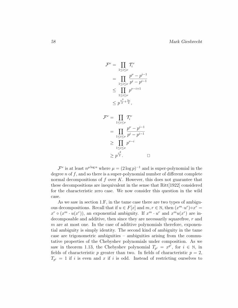
58 Mark Giesbrecht
Fν =∏
1≤i≤νT νi
=∏
1≤i≤ν
pν − pi−1
pi − pi−1
≤∏
1≤i≤νpν−i+1
≤ pν2
2+ 3ν
2 ,
Fν =∏
1≤i≤νT νi
=∏
1≤i≤ν
pν − pi−1
pi − pi−1
≥∏
1≤i≤νpν−i
≥ pν2
2 .
Fν is at least nµ logn where µ = (2 log p)−1 and is super-polynomial in thedegree n of f , and so there is a super-polynomial number of different completenormal decompositions of f over K. However, this does not guarantee thatthese decompositions are inequivalent in the sense that Ritt[1922] consideredfor the characteristic zero case. We now consider this question in the wildcase.
As we saw in section 1.F, in the tame case there are two types of ambigu-ous decompositions. Recall that if u ∈ F [x] and m, r ∈ N, then (xm ·ur)xr =xr (xm · u(xr)), an exponential ambiguity. If xm · ur and xmu(xr) are in-decomposable and additive, then since they are necessarily squarefree, r andm are at most one. In the case of additive polynomials therefore, exponen-tial ambiguity is simply identity. The second kind of ambiguity in the tamecase are trigonometric ambiguities – ambiguities arising from the commu-tative properties of the Chebyshev polynomials under composition. As wesaw in theorem 1.13, the Chebyshev polynomial Tpi = xp
i, for i ∈ N, in
fields of characteristic p greater than two. In fields of characteristic p = 2,Tpi = 1 if i is even and x if i is odd. Instead of restricting ourselves to

Functional Decomposition of Polynomials 59
equivalence under these two types of ambiguities, we define the more generalconcept of a permutation ambiguity. Two complete normal decompositionsare permutation equivalent if the composition factors of one are a permuta-tion of the composition factors of the other. Trigonometric ambiguities arecertainly encompassed in this definition. We now proceed to construct a classof polynomials which have a super-polynomial number (in their degrees) ofpermutation inequivalent decompositions over their splitting fields.
Theorem 3.12. Let p ∈ N be prime, ν ∈ N and F = GF (pν). Also, let Kbe an algebraic extension of F of degree pν over F . Then there exist simple
additive polynomials f ∈ K[x] of exponent ν which have Fν ≥ pν2
2 pairwisepermutation inequivalent complete normal decompositions in cSAPDECK
∗ .
Proof. Let (θ1, . . . , θν) be a basis for an algebraic extension F of Zp of degreeν. Also, let f = xp
ν − x ∈ F [x], and ε ∈ F (where F is an algebraic closureof F ) be algebraic of degree pν over F . Consider the polynomial f with rootsconsisting of all elements of K = F [ε] of the form εa for a ∈ F . The rootsof f have a basis (εθ1, . . . , εθν) over Zp. As in the construction of theorem
3.1, we now describe complete decompositions of f and f with respect to thebases (θ1, . . . , θν) and (εθ1, . . . , εθν). Let
Ψ1 = xp − θp−11 x ∈ F [x], and
Ψ1 = xp − (εθ1)p−1x ∈ K[x].
For i > 1, define
Ψi = (xp −Ψi−1(θi)p−1x) Ψi−1 ∈ F [x], and
Ψi = (xp − Ψi−1(εθi)p−1x) Ψi−1 ∈ K[x].
Then
f = Ψν =(xp −Ψν−1(θν)p−1x) · · · (xp − θp−1
1 x), and
f = Ψν =(xp − Ψν−1(εθν)p−1x) · · · (xp − (εθ1)p−1x).
Since, for 1 ≤ i ≤ ν,
Ψi =∏
(a1,...,ai)∈Zip
(x−∑
1≤j≤iajθjε) ,

60 Mark Giesbrecht
we find that
Ψi−1(εθi) =∏
(a1,...,ai−1)∈Zi−1p
(εθi −∑
1≤j≤i−1
ajθjε)
= εpi−1 ∏
(a1,...,ai−1)∈Zi−1p
(θi −∑
1≤j≤i−1
ajθj)
= εpi−1
Ψi−1(θi).
Thus, in any decomposition of f into p-linear components in K[x], for 1 ≤i ≤ ν, the ith composition factor has the form
xp − aεpi−1(p−1)x
for some a ∈ F . If any non-identity permutation of a decomposition was alsoa decomposition of f , then
aεpi−1(p−1) = bεp
j−1(p−1)
for some 1 ≤ i < j ≤ ν and a, b ∈ F . But then ε would satisfy a polynomialin F [x] of degree less than pν , giving a contradiction. It follows that for theclass of polynomials just constructed there are Fν permutation inequivalent,complete normal decompositions.
The above theorem gives a super-polynomial lower bound on the number ofpermutation inequivalent, complete normal decompositions possible for anarbitrary polynomial.
Theorem 3.13. Let p be a prime number, ν ∈ N, and n = pν . There existfields K of algebraic degree at most n log n over Zp, and monic polynomialsof degree n in K[x] which have nµ logn decompositions in cDECK
∗ whichare inequivalent up to exponential and permutation ambiguities (where µ =(2 log p)−1).
Proof. Let f ∈ AF be simple of degree n = pν as constructed in theorem3.11. By lemma 3.11 we know f has at least
pv2
2 = nµ logn
complete normal decompositions in K[x] (where µ = (2 log p)−1), and thesedecompositions are inequivalent up to exponential and permutation ambigu-ities. The field K in theorem 3.11 has degree νpν = O(n log n) over Zp.

Functional Decomposition of Polynomials 61
Additive polynomials are certainly not the only class of polynomials whichpotentially have a super-polynomial number (in their degrees) of inequiva-lent decompositions. For example, let Q be a set of additive polynomialswhich have a super-polynomial number of inequivalent decompositions intheir degrees (such as that defined in theorem 3.11). Define a new set ofpolynomials
D = g f g|f ∈ Q, g ∈ F [x], deg f = deg g = n.
Each f ∈ D has a super-polynomial number of decompositions in its degreeand yet D is not a set of additive polynomials.

62 Mark Giesbrecht
4 The Ring of Additive Polynomials
4.1 Basic Ring Structure
Ore[1933a] considers rings of polynomials RF ⊆ F [x] under the usual poly-nomial addition (+), and a (possibly non-commutative) multiplication (×).The only further assumption he makes is the existence of a degree functionδ : RF \ 0 → N such that if f, g ∈ RF with δ(f) = r and δ(g) = s, thenδ(f × g) = r + s. In Ore[1933b] he applies this theory to the ring AF of ad-ditive polynomials with composition as ring multiplication and exponent asthe degree function. In this chapter, in sections A-D we present a summaryof the theory of Ore as applied to additive polynomials. In section E we in-vestigate the uniqueness properties of decompositions, and some propertiesof the indecomposable composition factors. We also strengthen a theoremof Ore[1933a] as applied to additive polynomials. In section F we use therelationships between decompositions developed in the previous sections togive an upper bound on the number of complete rational decompositions ofan arbitrary additive polynomial. In chapter 5 we will then use the theorydeveloped here to construct decomposition algorithms for additive polyno-mials.
Recall from chapter 3 that if F is a field of characteristic p then f ∈ F [x]is additive if f(x + y) = f(x) + f(y) for independent indeterminates x andy. We denote the set of all additive polynomials over F as AF ⊆ F [x] and forf ∈ AF,
f =∑
0≤i≤νaix
pi
with ai ∈ F for 0 ≤ i ≤ ν and aν 6= 0. The integer ν ≥ 0 is called theexponent of f and we write expn f = ν. It is easy to see that AF is a ringwithout zero divisors. We will also show it has a right division algorithm (ie.if f, g ∈ AF, with g 6= 0, then there exists Q,R ∈ AF such that f = Q g +Rand expnR < expn g), and is therefore a left-Euclidean ring (the terminologyis derived from the fact that the right division algorithm makes it a principalleft ideal ring). Let f, g ∈ AF with g 6= 0 and expn f = ν, and expn g = ρ.Assume also that f and g have leading (high order) coefficients a ∈ F andb ∈ F respectively. If ν < ρ then division is trivial. If ν ≥ ρ then withf (ν) = f , define
h(ν) = ab−pν−ρxp
ν−ρ ∈ AF
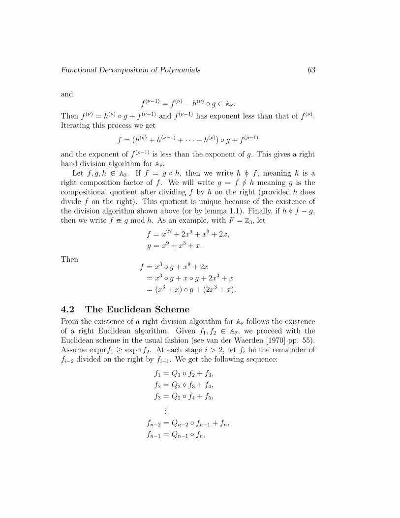
Functional Decomposition of Polynomials 63
andf (ν−1) = f (ν) − h(ν) g ∈ AF.
Then f (ν) = h(ν) g + f (ν−1) and f (ν−1) has exponent less than that of f (ν).Iterating this process we get
f = (h(ν) + h(ν−1) + · · ·+ h(ρ)) g + f (ρ−1)
and the exponent of f (ρ−1) is less than the exponent of g. This gives a righthand division algorithm for AF.
Let f, g, h ∈ AF. If f = g h, then we write h | f , meaning h is aright composition factor of f . We will write g = f / h meaning g is thecompositional quotient after dividing f by h on the right (provided h doesdivide f on the right). This quotient is unique because of the existence ofthe division algorithm shown above (or by lemma 1.1). Finally, if h | f − g,then we write f ≡ g mod h. As an example, with F = Z3, let
f = x27 + 2x9 + x3 + 2x,
g = x9 + x3 + x.
Thenf = x3 g + x9 + 2x
= x3 g + x g + 2x3 + x
= (x3 + x) g + (2x3 + x).
4.2 The Euclidean SchemeFrom the existence of a right division algorithm for AF follows the existenceof a right Euclidean algorithm. Given f1, f2 ∈ AF, we proceed with theEuclidean scheme in the usual fashion (see van der Waerden [1970] pp. 55).Assume expn f1 ≥ expn f2. At each stage i > 2, let fi be the remainder offi−2 divided on the right by fi−1. We get the following sequence:
f1 = Q1 f2 + f3,
f2 = Q2 f3 + f4,
f3 = Q2 f4 + f5,
...
fn−2 = Qn−2 fn−1 + fn,
fn−1 = Qn−1 fn,

64 Mark Giesbrecht
where Qi, fi ∈ AF and expn fi < expn fi−1. The number of steps n is at mostthe exponent of f2. The polynomial afn ∈ AF, where a ∈ F is such that afnis monic, is the greatest common (right compositional) divisor or meet of f1
and f2. We denote the meet f1 u f2. As an example, assume as before thatF = Z3 and
f1 = x27 + 2x9 + x3 + 2x,
f2 = x9 + x3 + x.
Following the Euclidean scheme,
f1 = (x3 + x) f2 + (2x3 + x),
f2 = (2x3 + x) (2x3 + x),
f3 = 2x3 + x.
Normalising to make the meet monic,
f1 u f2 = 2−1(2x3 + x)
= x3 + 2x.
The existence of a Euclidean algorithm means AF is a principal left idealring. Let f1 and f2 be two additive polynomials, and let (f1) and (f2) bethe left ideals generated by them. The ideal D = (f1) + (f2) consists of allsums of left multiples of f1 with left multiples of f2. Because AF is principal,D = (u) for some unique monic u ∈ AF and this u is the meet of f1 andf2. The set L = (f1) ∩ (f2) is also an ideal and consists of all common leftmultiples of f1 and f2. Assume f1f2 6= 0. We must now show that L 6= (0).Let D = f1 u f2. From the extended Euclidean scheme we know that thereexist A1, A2 ∈ AF such that A1 f1 +A2 f2 = D. If f2 = R2 D for R2 ∈ AF,then R2 A1 f1 +R2 A2 f2 = f2 and R2 A1 f1 = (x−R2 A2)f2. Thusf1 and f2 are both right factors of R2 A1 f1, and since this is nonzero,L 6= (0). The ring AF is a principal left ideal ring, so L = (h) for someunique monic h ∈ F [x]. This is the common left multiple of f1 and f2 ofleast exponent, which we will call the join of f1 and f2. We denote the joinof f1 and f2 by f1 t f2. Some properties of the join are summarised in thefollowing lemma.
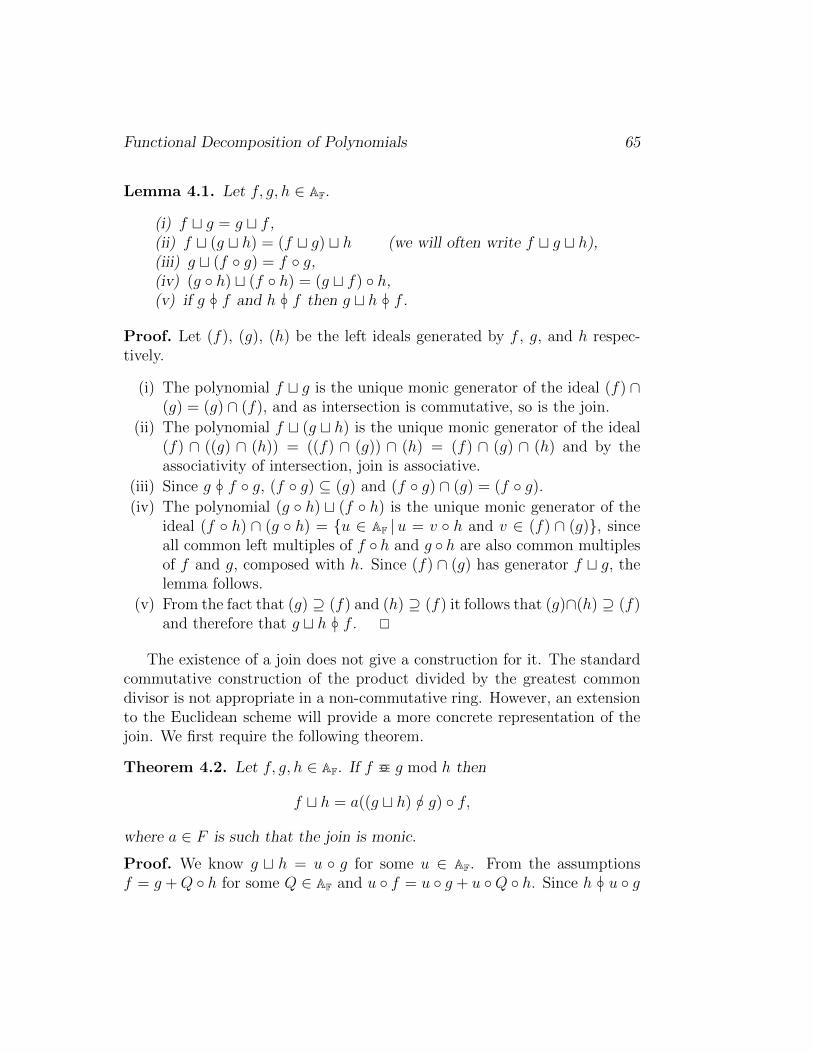
Functional Decomposition of Polynomials 65
Lemma 4.1. Let f, g, h ∈ AF.
(i) f t g = g t f ,(ii) f t (g t h) = (f t g) t h (we will often write f t g t h),(iii) g t (f g) = f g,(iv) (g h) t (f h) = (g t f) h,(v) if g | f and h | f then g t h | f .
Proof. Let (f), (g), (h) be the left ideals generated by f , g, and h respec-tively.
(i) The polynomial f t g is the unique monic generator of the ideal (f) ∩(g) = (g) ∩ (f), and as intersection is commutative, so is the join.
(ii) The polynomial f t (g t h) is the unique monic generator of the ideal(f) ∩ ((g) ∩ (h)) = ((f) ∩ (g)) ∩ (h) = (f) ∩ (g) ∩ (h) and by theassociativity of intersection, join is associative.
(iii) Since g | f g, (f g) ⊆ (g) and (f g) ∩ (g) = (f g).
(iv) The polynomial (g h) t (f h) is the unique monic generator of theideal (f h) ∩ (g h) = u ∈ AF |u = v h and v ∈ (f) ∩ (g), sinceall common left multiples of f h and g h are also common multiplesof f and g, composed with h. Since (f) ∩ (g) has generator f t g, thelemma follows.
(v) From the fact that (g) ⊇ (f) and (h) ⊇ (f) it follows that (g)∩(h) ⊇ (f)and therefore that g t h | f .
The existence of a join does not give a construction for it. The standardcommutative construction of the product divided by the greatest commondivisor is not appropriate in a non-commutative ring. However, an extensionto the Euclidean scheme will provide a more concrete representation of thejoin. We first require the following theorem.
Theorem 4.2. Let f, g, h ∈ AF. If f ≡ g mod h then
f t h = a((g t h) / g) f,
where a ∈ F is such that the join is monic.
Proof. We know g t h = u g for some u ∈ AF. From the assumptionsf = g +Q h for some Q ∈ AF and u f = u g + u Q h. Since h | u g
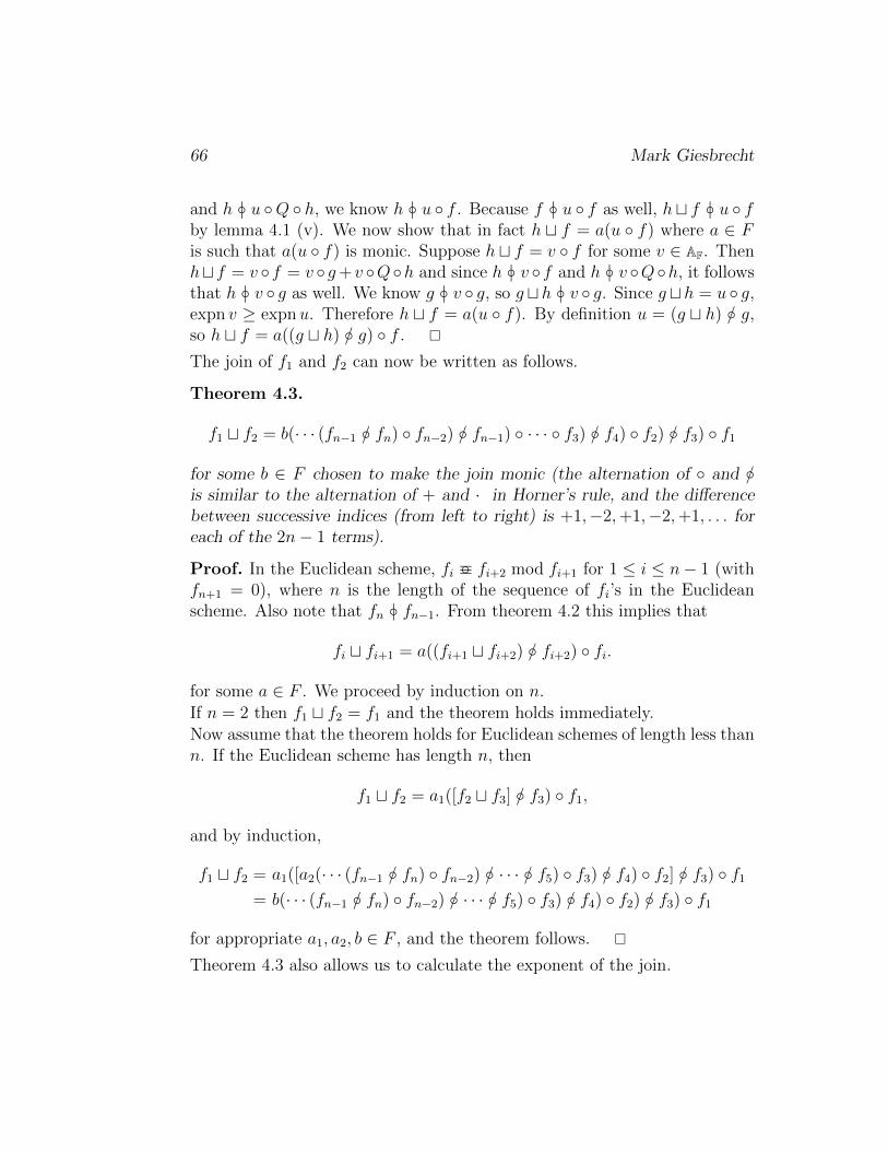
66 Mark Giesbrecht
and h | u Q h, we know h | u f . Because f | u f as well, ht f | u fby lemma 4.1 (v). We now show that in fact h t f = a(u f) where a ∈ Fis such that a(u f) is monic. Suppose h t f = v f for some v ∈ AF. Thenhtf = v f = v g+ v Qh and since h | v f and h | v Qh, it followsthat h | v g as well. We know g | v g, so g th | v g. Since g th = u g,expn v ≥ expnu. Therefore h t f = a(u f). By definition u = (g t h) / g,so h t f = a((g t h) / g) f .
The join of f1 and f2 can now be written as follows.
Theorem 4.3.
f1 t f2 = b(· · · (fn−1 / fn) fn−2) / fn−1) · · · f3) / f4) f2) / f3) f1
for some b ∈ F chosen to make the join monic (the alternation of and /is similar to the alternation of + and · in Horner’s rule, and the differencebetween successive indices (from left to right) is +1,−2,+1,−2,+1, . . . foreach of the 2n− 1 terms).
Proof. In the Euclidean scheme, fi ≡ fi+2 mod fi+1 for 1 ≤ i ≤ n− 1 (withfn+1 = 0), where n is the length of the sequence of fi’s in the Euclideanscheme. Also note that fn | fn−1. From theorem 4.2 this implies that
fi t fi+1 = a((fi+1 t fi+2) / fi+2) fi.
for some a ∈ F . We proceed by induction on n.If n = 2 then f1 t f2 = f1 and the theorem holds immediately.Now assume that the theorem holds for Euclidean schemes of length less thann. If the Euclidean scheme has length n, then
f1 t f2 = a1([f2 t f3] / f3) f1,
and by induction,
f1 t f2 = a1([a2(· · · (fn−1 / fn) fn−2) / · · · / f5) f3) / f4) f2] / f3) f1
= b(· · · (fn−1 / fn) fn−2) / · · · / f5) f3) / f4) f2) / f3) f1
for appropriate a1, a2, b ∈ F , and the theorem follows.
Theorem 4.3 also allows us to calculate the exponent of the join.

Functional Decomposition of Polynomials 67
Theorem 4.4. expn(f1 t f2) = expn f1 + expn f2 − expn(f1 u f2)
Proof. Using the simple fact that expn f g = expn f + expn g and expn f /g = expn f − expn g, for f, g ∈ AF, a quick examination of the formula forjoin given in theorem 4.3 reveals that
expn f1 t f2 = expn f1 + expn f2 − expn fn
= expn f1 + expn f2 − expn(f1 u f2)
and the theorem is proved.
Continuing with the previous example,
f1 t f2 = a((f2 / f3) f1)
= a(((2x3 + x) (2x3 + x)) / (2x3 + x)) f1
= a(2x3 + x) (x27 + 2x9 + x3 + 2x)
= a(2x81 + 2x27 + x9 + 2x3 + 2x)
= x81 + x27 + 2x9 + x3 + x.
For verification we check that indeed
x81 + x27 + 2x9 + x3 + x = (x9 + x) f2
= (x3 + 2x) f1.
If f, g, h ∈ AF with g 6= 0 and f = g h, then h is a multiplicative factoras well as a right composition factor of f . Thus, if
f = Q g +R
where Q,R ∈ AF and expnR < expn g, then
f −R = Q g= Q′g,
where Q′ = (f−R)/g ∈ F [x]. Therefore f = Q′g+R and usual multiplicativedivision in F [x] yields the same remainder as compositional division in AF.This means that the right-Euclidean algorithm for AF just described generatesthe same sequence of fi’s as the usual multiplicative Euclidean algorithm(though obviously a different sequence of Qi’s) and we have the followingtheorem.
68 Mark Giesbrecht
Theorem 4.5. If f1, f2 ∈ AF, then f1uf2 is equal to the usual multiplicativegreatest common divisor of f1 and f2.
We can speak of f1 and f2 in AF as being composition-coprime if f1uf2 =x, and this is equivalent to saying that the usual, multiplicative, greatestcommon divisor of f1 and f2 is x.
4.3 The Structure of the Set of DecompositionsThe set of all distinct complete rational normal decompositions of a givenadditive polynomial has a very strong internal structure. Ore[1933a] devel-ops this structure in the general context of non-commutative left-Euclideanpolynomial rings.
The central concept of Ore’s theory is that of transformation. Let f, g ∈AF be monic. The monic polynomial
g . f = (g t f) / g ∈ AF
is called the transformation of f by g. By theorem 4.4, we determine that
expn(g . f) = expn(g t f)− expn g
= expn g + expn f − expn(g u f)− expn g
= expn f − expn(g u f).
Obviously, if f and g are composition-coprime then expn(g . f) = expn f(though g . f certainly does not have to equal f).
The properties of transformation will be developed in the following fewtheorems. There does not seem to be an easy technique relating these prop-erties to the familiar multiplicative identities, say over the integers. Oncemight liken meet to integer greatest common divisor (gcd) and join to leastcommon multiple (lcm). In this case transformation becomes lcm divided bygcd. But this is also a commutative construction, which is not the case fortransformation in the additive polynomials.
Theorem 4.6. Let f, g, h ∈ AF be monic. If f ≡ g mod h then f .h = g .h.
Proof. By theorem 4.2, f th = ((g th) / g) f . Dividing both sides on theright by f , we get (f t h) / f = (g t h) / g (the multiplying constant a ∈ Ffrom theorem 4.2 is one since f, g and h are assumed to be monic). Directly,we have that f . h = g . h.

Functional Decomposition of Polynomials 69
Theorem 4.7. Let f, g, h ∈ AF be monic. If h | f g then
(i) (g . h) | f , and
(ii) if f is indecomposable, g u h = x, and h 6= x, then g . h = f .
Proof.
(i) The polynomials g and h are both right factors of f g, so there existsa u ∈ AF such that f g = u (g t h). Thus
f = (u (g t h)) / g= u (g . h).
(ii) As f is indecomposable and g u h = x, we know expn(g . h) = expnh.From (i), (g . h) | f and since expnh = expn(g . h) > 0 and f isindecomposable, (g . h) = f .
Two monic additive polynomials f, g ∈ AF are said to be similar if thereexists a u ∈ AF composition-coprime with g such that f = u . g. To denotesimilarity we write f ∼ g. Note that if f and g are similar then expn f =expn g. We will show that similarity is an equivalence relation. First, wemust prove a preliminary lemma.
Lemma 4.8. Let f, g, h ∈ AF be monic. Then (g h) . f = g . (h . f).
Proof.
(g h) . f = ((g h) t f) / (g h)
= ((g h) t h t f) / (g h)
= ((g h) t (h t f)) / h) / g= (g t ((h t f) / h)) / g= g . (h . f).

70 Mark Giesbrecht
Theorem 4.9. Similarity is an equivalence relation.
Proof. Let f, g, h ∈ AF be monic.
(i) Similarity is reflexive since x . f = f .
(ii) Assume f ∼ g, so that f = u . g for some u ∈ AF such that u u g = x.As u and g are composition-coprime, there exist Q, v ∈ AF such that
v u+Q g = x.
Therefore v u ≡ x mod g. We have
g = x . g = (v u) . g by theorem 4.6
= v . (u . g) by lemma 4.8
= v . f,
and g ∼ f , so similarity is symmetric.
(iii) Assume f ∼ g and g ∼ h. Then there exist u, v ∈ AF such thatu u g = x, f = u . g, v u h = x, and g = v . h. By lemma 4.8,
f = u . g
= u . (v . h)
= (u v) . h.
Because h and f have the same exponent, (u v) u h = x and h ∼ f .Thus similarity is transitive.
By (i), (ii), and (iii) above, similarity is an equivalence relation.
An interesting case is that of the additive polynomial xp, which has thefollowing property.
Lemma 4.10. The only additive polynomial similar to xp ∈ AF is xp.
Proof. Let u ∈ AF be monic and composition-coprime with xp. Thus, u issimple (u is monic and u(0) = 0). Since utxp = wxp for some w ∈ AF, utxpis not simple. We also know that u t xp = v u for some v = xp + ax ∈ AF
for some a ∈ F . As u is simple and v u is not simple, v = xp. Thereforeu t xp = xp u and u . xp = xp.
A further property of transformation is that the transformation of a join issimply the transformation of its components.

Functional Decomposition of Polynomials 71
Theorem 4.11. Let f, g, h ∈ AF be monic. Then h.(ftg) = (h.f)t(h.g).
Proof. We know
(h . (f t g)) h = ((h t (f t g)) / h) h= (h t (f t g))
= (h t f) t (h t g)
= (((h t f) / h) t ((h t g) / h)) h.
Dividing on the right by h we get
h . (f t g) = (h . f) t (h . g).
Transformation will later be used to characterise the different decompo-sitions of a given additive polynomial. It will be useful to know the effect oftransformation on a composition of additive polynomials.
Theorem 4.12. Let f, g, h ∈ AF be monic. Then h . (f g) = ((g . h) . f) (h . g).
Proof. We know that
h . (f g) = h . ((f g) t g)
= (h . (f g)) t (h . g) (by theorem 4.11)
= Q (h . g)
for some Q ∈ AF. This implies Q (h t g) = h t (f g) and
Q (g . h) = (h t (f g)) / g= (g t (h t (f g))) / g= g . (h t (f g))
= (g . h) t (g . (f g))
= (g . h) t ((g t (f g)) / g)
= (g . h) t f.
Therefore, Q = (g . h) . f and the theorem follows.
This theorem can be easily extended to consider the transformation of acomposition of many polynomials.

72 Mark Giesbrecht
Theorem 4.13. Let f ∈ AF be monic. Assume f = fmfm−1· · ·f1 wherefi ∈ AF are monic for 1 ≤ i ≤ m. Let h ∈ AF be monic and composition-coprime with f . If hi ∈ AF is defined by
hi = (fi−1 fi−2 · · · f1) . h for i > 1,
h for i = 1,
for 1 ≤ i ≤ m thenh . f = fm fm−1 · · · f1,
where fi = hi . fi.
Proof. We proceed by induction on m. If m = 1 then h . f1 = f1. Assumethe theorem is true if the number of factors is less than m and that m > 1.From theorem 4.12,
h . f = h . ((fm fm−1 · · · f2) f1)
= ((f1 . h) . (fm · · · f2)) (h . f1).
Since h and f are composition-coprime, expnh . f = expn f . Therefore, bycomputing the exponents of each side of the above equation, we have
expn(fm · · · f2) = expn((f1 . h) . (fm · · · f2)),
and (f1 . h) and fm · · · f2 must be composition-coprime. By induction,
(f1 . h) . (fm · · · f2) = fm fm−1 · · · f2
with fi = hi . fi for 2 ≤ i ≤ m where hi is defined by
hi =
(fi−1 fi−2 · · · f2) . (f1 . h) for i > 2
f1 . h for i = 2
= (fi−1 · · · f2) . h (by lemma 4.8),
and the theorem follows.
The above theorems consider the transformations of arbitrary decompo-sitions. What are the effects of transformation on complete decompositions?We first need to know the relationship between the decompositions of similaradditive polynomials.

Functional Decomposition of Polynomials 73
Theorem 4.14. If f, g ∈ AF, f ∼ g and f is indecomposable, then g isindecomposable.
Proof. Assume f = u . g for some u ∈ AF composition-coprime with g.Suppose that g = g2 g1, where expn g2 > 0 and expn g1 > 0 (so g isdecomposable). By theorem 4.12, f = ((g1.u).g2)(u.g1). The polynomialsu and g1 are composition-coprime because u and g are composition-coprimeand g1 | g. It follows that u . g1 ∼ g1 and expnu . g1 = expn g1. Thereforeexpn((g1.u).g2) = expn g2 and f is decomposable, a contradiction. Thereforeg is indecomposable.
From 4.13 and 4.14 we immediately get the following theorem.
Theorem 4.15. If (f, (fm, . . . , f1)) ∈ cAPDECF∗ and g ∼ f (say g = u.f),
then there exists (g, (gm, . . . , g1)) ∈ cAPDECF∗ where gi ∼ fi for 1 ≤ i ≤ m
(specifically, g1 = u . f1 for some u ∈ AF and gi = ((fi−1 · · · f1) . u) . fifor 2 ≤ i ≤ m).
Proof. By theorem 4.13 we transform the composition, giving a decomposi-tion of g. The fact that this is a complete decomposition follows from 4.14.
Transformation and similarity can be used to completely characterise therelationship between decompositions. Let f, g ∈ AF be monic. If there existsa monic f ∈ AF such that f ∼ f and f = g.f , we say f and g are transmutableor that they transmute. The additive polynomial f is called a transmutationof f by g. In this case,
f g = (g . f) g= ((g t f) / g) g= g t f= ((f t g) / f) f= (f . g) f= g f
where g = f . g ∈ AF. Because f ∼ f , f and f have the same exponent and
74 Mark Giesbrecht
so g and g also have the same exponent. We know
expn(f t g) = expn f + expn g − expn(f u g)
= expn(f g)
= expn(f g)
= expn f + expn g.
Thus expn f u g = 0 and g ∼ g.There is no reason why there cannot exist an f ∈ AF such that f ∼ f , f 6= fand f = g . f . The transmutation of f by g is not unique. Consider thefollowing example over an arbitrary field F of characteristic p.
f = xp + ax a ∈ Fg = xp + bx b ∈ F
Then f g = xp2
+ (a+ bp)xp + abx. Assume f g = g f where
f = xp + ax a ∈ Fg = xp + bx b ∈ F
This implies b+ ap = a+ bp and ab = ab. Thus
0 = ab− ab= ab− a(−ap + a+ bp)
= ab+ ap+1 − aa− bpa= a(b− a)− a(b− a)p
= (b− a)(a− a(b− a)p−1),
and either f = g and f = g, or a is a root of ϕ = a− x(b− x)p−1 ∈ F [x] (gis uniquely determined as g = (f g) / f)). Noting that
f = (g f) / g= (g t (g f)) / g since g | g f= g . (g f)
= g . ((g f) t f)
= g . (g f) t (g . f)
= f t (g . f),

Functional Decomposition of Polynomials 75
and expn f = expn g . f = 1, it follows that f = g . f , so f ∼ f andthe transmutation of f by g is f . Since the argument can be reversed, itimplies that the polynomial f can transmute by g in up to p different ways,depending upon the roots of ϕ in F .
A point worth noting is that xp does not transmute by xp. By lemma4.10, the only polynomial similar to xp is xp. If xp did transmute by xp, thenxp = xp . xp = (xp t xp) / xp = x, a contradiction.
The set of all complete decompositions of f ∈ AF can be given structureusing transmutation and similarity. Let (f, (fm, fm−1, . . . , f1)) ∈ cAPDECF
∗ .If fi and fi−1 fi−2 · · · f` transmute for some i, ` ∈ N with m ≥ i > ` ≥ 1then we get another complete decomposition of f . As in theorem 4.13, thisis
(f, (fm, fm−1, . . . , fi+1, fi−1, . . . , f`, fi, f`−1, . . . , f1)) ∈ cAPDECF∗ .
where fj ∼ fj for ` ≤ j ≤ i. We say these two decompositions are single-
transmutation equivalent. Letting (f, (f (0)m , . . . , f
(0)1 )) ∈ cAPDECF
∗ , if thereis a sequence
(f (0)m , . . . , f
(0)1 )
(f (1)m , . . . , f
(1)1 )
...
(f (t)m , . . . , f
(t)1 )
where (f, (f (i)m , . . . , f
(i)1 )) ∈ cAPDECF
∗ for 1 ≤ i ≤ t, and (f (i)m , . . . , f
(i)1 ) and
(f (i+1)m , . . . , f
(i+1)1 ) are single-transmutation equivalent for 1 ≤ i < t, we say
that f (0)m , . . . , f
(0)1 and f (t)
m , . . . , f(t)1 are transmutation equivalent. Transmu-
tation equivalence is the reflexive transitive closure of single-transmutationequivalence.
Theorem 4.16. All complete rational normal decompositions of a monicf ∈ AF are transmutation equivalent.
Proof. Let (f, (fm, . . . , f1)) = (f, (f (0)m , . . . , f
(0)1 )) and (f, (gr, . . . , g1)) for
r,m ∈ N be complete rational normal decompositions of f . We prove thetheorem by induction on m. If m = 1 then f is indecomposable and f1 = g1,so the statement is true.
76 Mark Giesbrecht
Assume the theorem is true for complete decompositions of length lessthan m. Let k ∈ N be the smallest number such that g1 | (fk fk−1 · · · f1).If k = 1 then f1 = g1 (they are both indecomposable), and by induction (f /g1, (fm, . . . , f2)) and (f / g1, (gr, . . . , g2)) ∈ cAPDECF
∗ are transmutationequivalent. Therefore (f, (fm, . . . , f1)) and (f, (gr, . . . , g1)) are transmutationequivalent.
If k > 1 then fk−1 fk−2 · · · f1 and g1 are composition-coprime. Bytheorem 4.7(ii),
fk = (fk−1 fk−2 · · · f1) . g1,
fk ∼ g1, and fk and (fk−1 · · · f1) are transmutable. Therefore
fk fk−1 · · · f1 = (g1 . (fk−1 · · · f1)) g1
= fk−1 fk−2 · · · f1 g1
by theorem 4.13, where fi ∼ fi for 1 ≤ i ≤ k − 1. Thus
(f, (fm, fm−1, . . . , fk+1, fk−1, . . . , f1, g1))
and (f, (fm, . . . , f1)) are single-transmutation equivalent. Also, by the induc-tive hypothesis, (f / g1, (fm, fm−1, . . . , fk+1, fk−1, . . . , f1)) and (f / g1, (gr, . . . , g2))are transmutation equivalent. Therefore (f, (fm, . . . , f1)) and (f, (gr, . . . , g1))are transmutation equivalent and the theorem follows.
Any two single-transmutation equivalent decompositions have the samenumber of indecomposable factors in any complete decomposition, and thesefactors are similar in pairs. Since similarity is transitive, we immediately getthe following corollary.
Corollary 4.17. Any two complete decompositions of f ∈ AF have thesame number of factors and if (f, (fm, fm−1, . . . , f1)), (f, (gm, gm−1, . . . , g1)) ∈cAPDECF
∗ for some m > 0, there exists a permutation σ of 1, . . . ,m suchthat gi ∼ fσi for 1 ≤ i ≤ m.
4.4 Completely Reducible Additive PolynomialsA monic additive polynomial is said to be completely reducible if it is thejoin of a set of indecomposable additive polynomials. Completely reducibleadditive polynomials have a number of nice properties which we will examinemathematically and algorithmically.

Functional Decomposition of Polynomials 77
Lemma 4.18. A completely reducible polynomial f ∈ AF can be representedin the form
f = hr t hr−1 t · · · t h1
where, for 1 ≤ i ≤ r, hi is indecomposable and no one of the hi’s is a rightcomposition factor of the join of the others. This is called an indecomposablebasis of f .
Proof. Let f ∈ AF be completely reducible and let u1, u2, . . . , um ∈ AF be theindecomposable right factors of f . We know that f is the join of these rightfactors by the definition of completely reducible, and that there is a finitenumber of them since they are all multiplicative divisors of f . Consider thefollowing method for determining an indecomposable basis for f .
1) Let T := ∅2) Let g(0) := x
3) For i from 1 to m
3.1) if ui u g(i−1) = x then
3.1.1) let g(i) := g(i−1) t ui3.1.2) let T := T ∪ ui
else
3.1.3) let g(i) := g(i−1)
3.2) if g(i) = f, then quit, returning T
At step 3.1, we know that if ui u g(i−1) 6= x then ui | g(i−1) for i ≥ 1because ui is indecomposable. In this case it will not change the join g(i−1)
and is redundant. Because f is the join of all its indecomposable right factors,g(k) = f for some k ≤ m. From the construction, the exponent of the joinof the polynomials in T is the sum of the exponents of these polynomials.By theorem 4.4, therefore, any one polynomial in T is composition-coprimewith the join of the others in T .
Note that we can choose any indecomposable right factor u1 we want in theabove procedure.
A polynomial f ∈ AF is said to be completely transmutable if in anycomplete decomposition, any two adjacent indecomposable factors are trans-mutable.

78 Mark Giesbrecht
Theorem 4.19. An additive polynomial is completely reducible if and onlyif it is completely transmutable.
Proof. We first show that if f ∈ AF is completely reducible then it is com-pletely transmutable. We proceed by induction on the number of indecom-posable factors in a complete decomposition of f . Assume f = g1 ∈ AF,where g1 is indecomposable. Then f is completely transmutable. Now, as-sume the statement is true if f has less than m indecomposable factors in anycomplete decomposition. Let f = gm gm−1 · · · g1 = g g1 where gi ∈ AF
are indecomposable for 1 ≤ i ≤ m and m > 2, and g = f / g1 ∈ AF. Asf is completely reducible, it has an indecomposable basis g1, h2, h3, . . . , h`with hi ∈ AF indecomposable for 2 ≤ i ≤ `. We get
g = ((h` t · · · t h2) t g1) / g1
= g1 . (h` t · · · t h2)
= (g1 . h`) t (g1 . h`−1) t · · · t (g1 . h2)
and g ∼ (h`t· · ·th1). Thus, g is completely reducible and, by the inductiveassumption, completely transmutable. We have shown the leftmost m − 1factors of any complete decomposition of f are completely transmutable.Now we need only show that g1 and g2 are transmutable. We know g2 |g = g1 . (h` t · · · t h2). By theorem 4.15, all complete decompositions ofg1 . (h` t · · · t h2) are simply decompositions of h` t · · · t h2 transformed byg1 (g1 and (h` t · · · t h2) are composition-coprime). Therefore, g2 = g1 . ufor some u ∈ AF similar to g2, and g1 and g2 are transmutable. Thus, anycompletely reducible additive polynomial is completely transmutable.
We now show that if f ∈ AF is completely transmutable then f is com-pletely reducible. Once again we prove this by induction on the number ofindecomposable factors in a complete decomposition of f . If f = g1, whereg1 ∈ AF is indecomposable, then f is obviously completely reducible. Assumethe statement holds if f has fewer than m factors in a complete decompo-sition. Then assume f = gm gm−1 · · · g1 where gi ∈ AF for 1 ≤ i ≤ m.Also, let g = gm gm−1 · · · g2. Since g is completely transmutable, it iscompletely reducible by the inductive assumption, so g = h` t · · · th2 where` ∈ N is greater than two and h2, . . . , h` ∈ AF are indecomposable. Eachof the hi are indecomposable right factors of g and because f is completelytransmutable, each of the hi’s can be transmuted with g1. Thus, hi = g1 . hi

Functional Decomposition of Polynomials 79
for some hi ∈ AF, hi ∼ hi for 1 ≤ i ≤ `. Therefore
f = g g1 = (h` t h`−1 t · · · t h2) g1
= ((g1 . h`) t (g1 . h`−1) t · · · t (g1 . h2)) g1
= h` t h`−1 t · · · t h2 t g1,
and since the hi are indecomposable for 2 ≤ i ≤ ` and g1 is indecomposable,f is completely reducible.
Note that since xp does not transmute with itself, this theorem impliesthat any completely reducible polynomial can have at most one compositionfactor xp in an arbitrary complete decomposition.A strong relationship exists between the composition factors of an arbitrarycomplete decomposition and an arbitrary indecomposable basis.
Theorem 4.20. Let f ∈ AF be completely reducible, (f, (fm, fm−1, . . . , f1)) ∈cAPDECF
∗ , and h1, . . . , h` be an indecomposable basis for f . Then m = `and there exists a permutation σ of 1, . . . ,m such that hi ∼ fσi for1 ≤ i ≤ m.
Proof. We proceed by induction on m. If m = 1, then f is indecomposable,and ` = 1 and σ is the identity permutation. Now assume the hypothesis istrue for all complete decompositions of length less than m. Let f ∈ AF becompletely reducible, (f, (fm, fm−1, . . . , f1)) ∈ cAPDECF
∗ , and h1, . . . , h` bean indecomposable basis for f . Since h1 is an indecomposable right factorof f , there exists a decomposition (f, (f ′m, f
′m−1, . . . , f
′2, h1)) ∈ cAPDECF
∗and by corollary 4.17 a permutation τ of 1, . . . ,m such that f ′i ∼ fτi for1 ≤ i ≤ m. Now, (f / h1, (f
′m, f
′m−1, . . . , f
′2)) ∈ cAPDECF
∗ and by theinductive assumption,
f / h1 = h1 t (h` t h`−1 t · · · t h2) / h1
= h1 . (h` t h`−1 t · · · t h2)
= (h1 . h`) t (h1 . h`−1) t · · · t (h1 . h2),
giving an indecomposable basis for f / h1. By the inductive hypothesis`− 1 = m− 1 so m = ` and there exists a permutation µ of 2, . . . ,m suchthat hi ∼ f ′µi for 2 ≤ i ≤ m. Extending this to a permutation µ of 1, . . . ,mby letting µ1 = 1 we find that σ = τ µ has the property that hi ∼ f ′µi ∼ fσifor 1 ≤ i ≤ m.

80 Mark Giesbrecht
4.5 The Uniqueness of TransmutationA question which will concern us algorithmically is that of the uniquenessof transmutation. We can characterise how additive polynomials trans-mute in terms of the similar factors in an arbitrary complete decomposi-tion. Let g ∈ AF be monic of exponent ν with complete decomposition(g, (gm, gm−1, . . . , g1)) ∈ cAPDECF
∗ . Let f ∈ AF be monic and indecompos-able. Assume that f transmutes by g in two distinct ways, say f = g . ffor f ∈ AF, f ∼ f , and f = g . f for f ∈ AF, f ∼ f , and f 6= f . Thenf g has complete decompositions (f g, (gm, . . . , g1, f)) where gi ∈ AF andgi ∼ gi for 1 ≤ i ≤ m and (f g, (gm, . . . , g1, f)) where gi ∈ AF and gi ∼ gi for1 ≤ i ≤ m. We know f | f g. Let k ∈ N be the smallest number such thatf | gkgk−1· · ·g1f (f does not divide f). Then f and gk−1gk−2· · ·g1fare composition-coprime and by theorem 4.7, gk = (gk−1 · · · g1) . f andgk ∼ f . We have the following theorem:
Theorem 4.21. Let f, g ∈ AF be monic with (g, (gm, . . . , g1)) ∈ cAPDECF∗
and f indecomposable. If f and g transmute in two or more distinct ways,then f ∼ gi for some i such that 1 ≤ i ≤ m.
We can further characterise when non-unique transmutations occur byshowing the following theorem about transmutations in general.
Theorem 4.22. Let f, g, h ∈ AF be monic. If f transmutes by g h withtransmutation f , then f and g transmute, and if a transmutation of f by gis f , then f and h transmute as well.
Proof. If f = (g h). f , then f = g . (h. f) by lemma 4.8. Since f and g hare composition-coprime, f and h are composition-coprime. Let f = h . f .Then f transmutes with g since f = g . f . Furthermore, because f = h . f ,f and h transmute.
This theorem can be extended to the case when f transmutes by hm hm−1 · · · h1.
Theorem 4.23. Let f, hi ∈ AF for 1 ≤ i ≤ m. If f transmutes by h =hm hm−1 · · · h1, then
(i) f transmutes by hm, with transmutation f (m) ∈ AF, for some f (m) ∼f , and
(ii) for m ≥ i > 1, f (i) transmutes by hi−1 with transmutation f (i−1) ∈AF for some f (i−1) ∼ f .
Functional Decomposition of Polynomials 81
Proof. We proceed by induction on m. The base case, where m = 2 followsdirectly from theorem 4.22. Assume the theorem holds if h is given as acomposition of less than m factors. If h is given as a composition of mfactors then by theorem 4.22 f transmutes by hm . Let f (m) ∈ AF be thetransmutation of f by hm. Also by theorem 4.22, f (m) transmutes withhm−1 · · · h1. By the inductive hypothesis, f (m) transmutes by hm−1 withsome transmutation f (m−1) ∼ f and for m − 1 ≥ i > 1, f (i) transmutes byhi−1 with some transmutation f (i−1) ∼ f (m) ∼ f .
If f transmutes by h in two distinct ways, then for an arbitrary decom-position (h, (hm, hm−1, . . . , h1)) ∈ cAPDECF
∗ , f transmutes by each hi inturn for m ≥ i ≥ 1. Which transmutation of f by h is obtained is deter-mined entirely by the transmutation of f (i) by hi for 1 ≤ i ≤ m. Since thetransmutation of f (i) by hi is unique if f (i) hi, the transmutation of f byh is determined completely by the transmutation of f (i) by hi for 1 ≤ i ≤ mwhen f (i) ∼ hi. With this in mind, we define an additive polynomial f ∈ AF
to be similarity free if in an arbitrary complete decomposition, no two of thecomposition factors are similar. In a similarity free additive polynomial, alltransmutations of the factors are unique.
The previous theorem also allows us to strengthen theorem 4.16 of Ore’s.We say two complete decompositions (f, (fm, fm−1, . . . , f1)) and (f, (gm, . . . , g1))in cAPDECF
∗ are single-indecomposable-transmutation equivalent if fi = gifor 1 ≤ i ≤ m or there exists an ` ∈ N with 1 ≤ ` < m such that
(f, (gm, . . . , g`+1, g`, g`−1, g`−2, . . . , g1)) = (f, (fm, . . . , f`+1, f`−1, f`, f`−2, . . . , f1))
where f` ∼ f` is the transmutation of f` by f`−1 and f`−1 = f` . f`−1 ∼ f`−1.
We define indecomposable-transmutation equivalence as the reflexive tran-sitive closure of single-indecomposable-transmutation equivalence. Thus, twodecompositions are indecomposable-transmutation equivalent if one can beobtained from the other by a sequence of transmutations of adjacent inde-composable factors.
Theorem 4.24. Two complete decompositions are indecomposable- trans-mutation equivalent if and only if they are transmutation equivalent.
Proof. If two complete decompositions are indecomposable-transmutationequivalent, then they are transmutation equivalent. By theorem 4.23, any
82 Mark Giesbrecht
transmutation of an indecomposable additive polynomial with a composi-tion of indecomposable polynomials is equivalent to a sequence of trans-mutations with each of the indecomposable factors in turn. Thus, single-transmutation equivalent decompositions are indecomposable-transmutationequivalent. Since transmutation equivalence is just the reflexive transitiveclosure of single-transmutation equivalence, transmutation equivalent decom-positions must be indecomposable-transmutation equivalent.
As an immediate corollary we get a stronger version of theorem 4.16.
Corollary 4.25. All complete decompositions of an additive polynomial f ∈AF in cAPDECF
∗ are indecomposable-transmutation equivalent.
From now on we will simply say two complete decompositions are transmu-tation equivalent to mean indecomposable-transmutation equivalent.
4.6 The Number of Complete DecompositionsUsing the methods from chapter 3 as well as the material from this chapter,we can now prove an upper bound on the number of complete decompositionsof a (not necessarily simple) additive polynomial.
Let f ∈ AF be monic of degree n = pν . Then f = g xp` where g ∈ AF
is simple and ` ≥ 0. From theorem 3.10, we know that g has at most nµ logn
complete decompositions in cSAPDECF∗ where µ = (2 log p)−1. For each
decomposition (g, (gm, gm−1, . . . , g1)) ∈ cSAPDECF∗ , f has a decomposition
(f, (gm, gm−1, . . . , g1,
` times︷ ︸︸ ︷xp, xp, . . . , xp)) ∈ cAPDECF
∗ .
Without changing the order of the gi’s for m ≥ i ≥ 1, and allowing fortransformations into similar factors, we can distribute the indecomposablefactors xp throughout the decomposition of f . There are up to(
m+ `
`
)≤(ν
`
)≤ 2ν ≤ n
such distributions. We know these are all the decompositions because all de-compositions of additive polynomials are transmutation equivalent. Becausethere are nµ logn complete decompositions of g ∈ cSAPDECF
∗ , there are atmost n1+µ logn complete decompositions of f ∈ cAPDECF
∗ . We have shownthe following generalisation of lemma 3.10.
Functional Decomposition of Polynomials 83
Theorem 4.26. If f ∈ AF has degree n, then f has at most n1+µ logn decom-positions in cAPDECF
∗ .
Note that in the case of a perfect field F , for any u ∈ AF, we know
u xp = xp u1p = xp u where u = u
1p xp ∈ AF. In this case there are,
therefore, exactly(m+``
)times as many complete decomposition of f than of
g in cAPDECF∗ .

84 Mark Giesbrecht
5 Decomposing Additive Polynomials5.1 The Model of ComputationThe model of computation used in this chapter is the “arithmetic Booleancircuit” as described in chapter 2, section A. Once again, let SF (n) be thenumber of field operations required to factor an arbitrary univariate poly-nomial f ∈ F [x] of degree n into irreducible factors (where F is a fieldof characteristic p). In this chapter, SF (n) is assumed to be polynomiallybounded. It is also assumed to satisfy the property that for p, ν ∈ N,∑
0≤i≤νSF (pi) = O(SF (pν)).
The following theorem will also be useful in the analysis of some of ouralgorithms.
Lemma 5.1. If p, ν, d ∈ N with p ≥ 2 and ν ≥ 1, then∑1≤i≤ν
idpi ≤ 3νdpν .
Proof. We proceed by induction on ν. If ν = 1 then the theorem is triviallytrue. Assume it is true for ν < k. Then∑
1≤i≤kidpi =
∑1≤i≤k−1
idpi + kdpk
≤ 3(k − 1)dpk−1 + kdpk
≤ (3/2)kdpk + kdpk
≤ 3kdpk,
and the theorem holds for all ν ≥ 1.
5.2 The Cost of Basic Operations in AF.Let f, g ∈ AF be of exponents ν and ρ respectively, and max(ν, ρ) ≤ δ. Thefollowing analyses of the basic operations in AF are probably not optimal,but will be sufficient for our purposes.
Lemma 5.2. (Composition) Computing f g requires at most O(δ2 log p)field operations.
Functional Decomposition of Polynomials 85
Proof. Each coefficient of g must be raised to the pith power for 0 ≤ i ≤ν ≤ δ. This requires O(ρδ log p) = O(δ2 log p) field operations.
Lemma 5.3. (Division with remainder) If g 6= 0, computing Q,R ∈ AF suchthat f = Q g+R and expnR < expn g requires O(δ2 log p) field operations.
Proof. The cost of computing right division with remainder is dominated bythe cost of raising g (and hence each coefficient of g) to the pith power for 0 ≤i ≤ ν − ρ. This requires O(ρ(ν − ρ) log p) = O(δ2 log p) field operations.
Lemma 5.4. (Meet) Computing f u g requires O(δ3 log p) field operations.
Proof. In the Euclidean scheme described in the previous section, each stepinvolves right division with remainder of additive polynomials with exponentat most δ. There are at most δ steps. Therefore we can compute the meetof f and g with O(δ3 log p) divisions.
Lemma 5.5. (Join) Computing f t g requires O(δ3 log p) field operations.
Proof. Using the formula of theorem 4.3, we must first compute the fi’s of theEuclidean scheme. This requires O(ν3 log p) field operations by the previouslemma. Computing the join then requires at most δ divisions and δ composi-tions of polynomials with exponents not exceeding 2δ. Thus, computing thejoin requires O(δ3 log p) + δO((2δ)2 log p) = O(δ3 log p) field operations.
Lemma 5.6. (Transformation) Computing f . g requires O(δ3 log p) fieldoperations.
Proof. By definition f . g = (f t g) / f , and the number of field operationsinvolved is dominated by the number of field operations required to computethe join, which is O(δ3 log p).
5.3 The Minimal Additive MultipleLet f be an arbitrary monic polynomial in F [x]. A concept which will proveextremely useful when dealing computationally with additive polynomials isthat of the minimal additive multiple f ∈ AF of f . This is the monic additivepolynomial of smallest exponent such that f is a multiple of f . The idea ofa minimal additive multiple first appears in Ore[1933b].
If f = 0, then f = f = 0 ∈ AF. If f ∈ PF does not equal zero, thefollowing algorithm computes the minimal additive multiple f of f .

86 Mark Giesbrecht
MinAddMult : PF → AF
Input: - f ∈ PF of degree n ≥ 1.
Output: - f ∈ AF, the minimal additive multiple of f.
1) For i from 0 to n,
1.1) compute hi ≡ xpi
mod f
where hi ∈ F [x] and deg hi < deg f.
2) Let k ∈ N be the smallest number with 0 ≤ k ≤ n
such that there exists α0, α1, . . . , αk−1 ∈ Fsuch that hk =
∑0≤j<k αjhj.
3) Return f = xpk −∑0≤j<k αjx
pj.
We know f is a multiple of f because
f = xpk −
∑0≤j<k
αjxpj
≡ (hk +∑
0≤j<kαjhj) mod f
≡ 0 mod f.
The existence of any additive multiple of f with exponent ` < k would implyh0, . . . , h` are linearly dependent, which is false. Thus f is the minimaladditive multiple of f . We know a solution always exists since n+ 1 vectorsin F n must be linearly dependent.
The number of field operations to compute hj for 0 ≤ j ≤ n isO(nM(n) log p).The determination of k can be done by a modified Gaussian elimination onthe n × n matrix H where Hij is the coefficient of xi in hj for 0 ≤ i, j < n.We proceed in stages from 0 to n − 1. Let H(0) = H. At stage ` (with0 ≤ ` < n) we perform Guassian elimination on rows zero through ` of H(k)
obtaining H(k+1) (leaving rows ` + 1 through n − 1 unchanged). If, at theend of stage `, row ` of H(`+1) has all entries zero, then rows zero through `of H are linearly dependent and we can return k = `. At each stage of thiselimination we only perform a row operation on row `, so each stage requiresO(n2) field operations over F . The complete procedure then requires O(n3)field operations. Given k, it is simple linear algebra to find α0, α1, . . . , αk−1
such that hk =∑
0≤j<k αjhj. This also require O(n3) field operations. Weget the following theorem:

Functional Decomposition of Polynomials 87
Theorem 5.7. Let f ∈ F [x] be monic of degree n. The minimal additivemultiple f ∈ AF of f can be determined in O(n3) field operations.
If f is also an additive multiple of f , then by theorem 4.5, h = f u fis equal to the multiplicative greatest common divisor of f and f . Thus fdivides f u f and this is an additive multiple of f . But f is the minimaladditive multiple of f so f = f u f and f | f . We have shown the following:
Theorem 5.8. If f ∈ AF is the minimal additive multiple of f ∈ F [x] andf is a monic additive multiple of f , then f | f .
Another characterisation of the minimal additive multiple of f ∈ PF canbe obtained by looking at the roots of f in its splitting field K. Assume f issquarefree and has roots θ1, . . . , θn and minimal additive multiple h. Thenf must have an additive multiple g ∈ AK such that
g = ((xp − θp−11 x) t (xp − θp−1
2 x) t · · · t (xp − θp−1n x)) ∈ AK .
The polynomial g is an additive multiple of f because all roots of f areroots of g, and g is additive. Also, g | h because for each root θi of f , kθimust be a root of h for each k ∈ Zp and 1 ≤ i ≤ n. The one dimensionalvector space Vi = kθi | k ∈ Zp is a subspace of the kernel of h, and thepolynomial gi = xp − θp−1
i x has Vi as its kernel. So gi | h for 1 ≤ i ≤ nand therefore g = (g1 t g2 t · · · t gn) | h as well (see lemma 4.1(v)). Thecoefficients of g are symmetric functions (over F ) of the θi’s for 1 ≤ i ≤ n.Each automorphism of K relative to F carries the set of roots of f intoitself. Thus, each automorphism leaves the coefficients of g fixed, and thesecoefficients must therefore be in F . It follows that g ∈ F [x], and since gright divides h (the minimal additive multiple of f), g is equal to h. Thisalso means that the exponent of the minimal additive multiple f is exactlythe dimension of the linear span of the roots of f considered as a Zp vectorspace in K.
An interesting case is when f is a normal polynomial in Zp[x] (a normalpolynomial is an irreducible polynomial such that its roots [in some fixedalgebraic closure of Zp] form a basis over Zp for its splitting field). Thedimension of the Zp vector space spanned by the roots of f is thereforethe degree of f . It follows that the normal polynomials of degree n areexactly those irreducible polynomials whose minimal additive multiples haveexponent n.
88 Mark Giesbrecht
5.4 Complete Rational Decomposition of Additive PolynomialsAssume the field F supports a polynomial factorisation algorithm. The pre-ceding method for finding minimal additive multiples can be used to build apolynomial time algorithm for finding rational complete normal decomposi-tions of additive polynomials in a polynomial number of field operations.
First we present an algorithm for finding the set of indecomposable rightcomposition factors of f ∈ AF.
FindIndecRightFactors: AF → P(AF)Input: - f ∈ AF, a monic additive polynomial.
Output: - H = h1, . . . , h`, the set of indecomposable
right composition factors of f.1) Factor f such that f = xe0he11 h
e22 · · ·hemm
where hi ∈ F [x] are distinct, monic and irreducible and
ei ∈ N \ 0 for 0 ≤ i ≤ m.
2) Let J := h | h is the minimal additive multiple of
hi for some i such that 1 ≤ i ≤ `.Assume J = g1, . . . , g` for some ` ∈ Nand is indexed such that if i < j then expn gi ≤ expn gjfor 1 ≤ i ≤ `.
3) For 1 ≤ i < j ≤ `, if gi | gj, mark gj.4) Let H = g ∈ J | g not marked in step 3.5) Return H.
To show correctness we must prove that g ∈ H if and only if g is anindecomposable right composition factor of f . If g ∈ AF is an indecomposableright factor of f , then, since g is also a multiplicative factor of f , eachirreducible multiplicative factor h ∈ F [x] of g is an irreducible multiplicativefactor of f . We know that the minimal additive multiple h ∈ AF of any such hright divides g by theorem 5.8, and as g is indecomposable, h = g. Thereforeg will never be marked in step 3 and g ∈ H. Assume, on the other hand, thatg ∈ H. Suppose that g is decomposable and h is an indecomposable rightcomposition factor of g. Then h is an indecomposable right factor of f andh ∈ H as shown above. In step 3, g would be marked as decomposable andwould not be in H, a contradiction. Therefore, each g ∈ H is indecomposableand the algorithm works correctly.
We now analyse the number of field operations required by the procedureFindIndecRightFactors. For f ∈ AF of degree n = pν consider computing
Functional Decomposition of Polynomials 89
FindIndecRightFactors(f). The factorisation in step 1 requires O(SF (n))field operations. In step 2 we find additive multiples of each of the indecom-posable right factors of f . The worst case occurs when there is one factor ofdegree n − 1. Thus, step 2 requires O(n3) field operations. The number ofoperations required in the remaining steps is dominated by the requirementsof steps 1 and 2, so we have the following:
Lemma 5.9. Given f ∈ F [x] of degree n we can compute all the indecom-posable right factors of f in O(SF (n) + n3) field operations.
Now consider the following algorithm for generating a complete decom-position of f in cAPDECF
∗ .
CompleteDecomposition: AF → cAPDECF∗
Input: - f ∈ AF, a monic additive polynomial.
Output: - a complete decomposition of f in cAPDECF∗ .
1) Using FindRightIndecFactors, find the set H of
indecomposable right factors of f. Assume
H = h1, . . . , h`.2) If h1 = f
then f is indecomposable, Return (f, (f)).
else
2.1) Let D :=CompleteDecomposition(f / h1).
We know D = (f / h1, (ut, . . . , u1)) ∈ cAPDECF∗
for some t ∈ N \ 0.2.2) Return (f, (ut, . . . , u1, h1)).
At each recursive stage of the algorithm we simply determine one in-decomposable right factor h1 of f . We then proceed recursively to find acomplete decomposition of f / h1. As f has exponent ν, and each inde-composable right factor has exponent at least one, there can be at most νrecursive stages. We now analyse the number of field operations requiredto decompose a polynomial f ∈ AF of degree n = pν . The worst case oc-curs when a p − linear (exponent one) right composition factor occurs ateach recursive stage i, for 1 ≤ i ≤ ν. In this case, at stage i we must callFindRightIndecFactors on a degree pi polynomial, requiring O(SF (pi)+p3i)field operations. Thus, the total number of field operations required to find

90 Mark Giesbrecht
one complete decomposition is∑0≤i≤ν
(SF (pi) +O(p3i)) = O(SF (pν) + p3ν)
= O(SF (n) + n3).
Theorem 5.10. Given an additive polynomial f ∈ AF of degree n we candetermine a complete decomposition of f in cAPDECF
∗ in O(SF (n) + n3)field operations.
Corollary 5.11. Rational indecomposability of an additive polynomial ofdegree n can be determined in O(SF (n) + n3) field operations.
5.5 General Rational Decomposition of Additive PolynomialsLet f ∈ AF be of degree n and let ℘ = (rm, rm−1, . . . , r1) be an orderedfactorisation of n. The fact that we can obtain a complete decompositionof an f ∈ cAPDECF
∗ in a polynomial number of field operations in n doesnot mean that we can determine the existence of a decomposition of f inAPDECF
℘ , and find one if it exists, in polynomial time. We can look at theset of all complete decompositions and check if the composition factors ofany of them can be “grouped” according to the desired ordered factorisation℘. More generally, a length d ordered factorisation κ = (sd, sd−1, . . . , s1) ofn ∈ N is said to be a refinement of a length m ≤ d ordered factorisation ℘ =(rm, rm−1, . . . , r1) if there exists a non-decreasing, onto map ϕ : 1, . . . , d →1, . . . ,m such that for 1 ≤ j ≤ m,∏
1≤i≤dϕ(i)=j
si = rj.
This is simply saying that the d-tuple κ can be divided into m contiguouspieces, with the elements of piece j having product rj, for 1 ≤ j ≤ m. Oneapproach to finding decompositions of f with a given ordered factorisation isto generate the set of all complete decompositions of f and check if any of theordered factorisations associated with these decompositions are a refinementof ℘.
We now present an algorithm for generating all the complete decomposi-tions of an additive polynomial.

Functional Decomposition of Polynomials 91
AllCompleteDecomposition: AF → P(cAPDECF∗ )
Input: - f ∈ AF, a monic additive polynomial.
Output: - the set of all complete decompositions of f
in cAPDECF∗ .
1) Using FindRightIndecFactors, find the set H of
indecomposable right factors of f. Assume
H = h1, . . . , h`.2) If f = h1
Then f is indecomposable, Return (f, (f)).
Else
2.1) Let T := ∅.2.2) For i from 1 to `
2.2.1) Let D(i) :=CompleteDecomposition(f / hi),the set of all complete decompositions
of (f / hi) in cAPDECF∗ .
2.2.2) For each decomposition
(f / hi, (u`, . . . , u1)) ∈ D(i),
add (f, (u`, . . . , u1, hi)) ∈ cAPDECF∗
to T.
2.3) Return T.
Correctness is easy to verify. At each recursive stage we simply find the setof all indecomposable right factors H of f and for each h ∈ H we recursivelyfind the complete decompositions of f / h. All complete decompositions arefound and, since we choose a different member of H in each step 2.2.1, eachdecomposition added to T is distinct.
We analyse the cost of the algorithm by first finding the cost of computingone complete decomposition. We then use the bounds developed in chapter 3and 4 on the number of complete decompositions to get bounds on the cost ofcomputing all complete decompositions. As with CompleteDecomposition,the worst case occurs when a p − linear right composition factor occurs ateach recursive stage i, for 1 ≤ i ≤ ν. In this case, at stage i, we must callFindRightIndecFactors on a degree pi polynomial, requiring O(SF (pi)+p3i)field operations. Thus the total number of field operations required to find

92 Mark Giesbrecht
one complete decomposition is∑0≤i≤ν
SF (pi) +O(p3i) = O(SF (pν) + p3ν)
= O(SF (n) + n3).
Theorem 5.12. If f ∈ AF is monic of degree n and t ∈ N, then we candetermine if there exist t decompositions of f in cAPDECF
∗ , and if so findthem, with O(t(SF (n) + n3)) field operations.
By theorem 4.26, the total number of complete normal decompositions off in cAPDECF
∗ is nO(logn), so we can compute all complete rational decom-positions of an arbitrary additive polynomial in a quasi-polynomial numberof field operations.
Let ℘ be a given ordered factorisation of n. As we generate each completedecomposition of f , we can check if the ordered factorisation associated withit is a refinement of ℘. The number of operations required to do this is dom-inated by the other steps in the algorithm. Thus, the number of operationsrequired to find all decompositions of f in DECF
℘ is of the same order as thenumber required to generate all complete decompositions.
Corollary 5.13. If f ∈ AF is monic of degree n, and ℘ is an ordered fac-torisation of n, then all decompositions of f in APDECF
℘ can be found in
nO(logn) field operations.
Note that this algorithm requires a comparable number of operations tothose of Kozen and Landau[1986] for separable irreducible polynomials.
5.6 General Decomposition of Completely ReducibleAdditive Polynomials
We now consider computing decompositions of a completely reducible addi-tive polynomial f ∈ AF of degree n corresponding to a given ordered factori-sation ℘ of n. We will see that the decomposition problem for completelyreducible additive polynomials can be computed in a polynomial number offield operations in the input degree. We proceed by constructing an inde-composable basis for f (see chapter 4, section D) and combine the basiscomponents appropriately to determine if an appropriate decomposition ex-ists, and if so, find it.

Functional Decomposition of Polynomials 93
We now describe an efficient way of computing an indecomposable basisfor a given completely reducible additive polynomial. The procedure stronglyresembles the one described in the proof of lemma 4.18.
IndecBasis: AF → AF∗
Input: f ∈ AF, completely reducible of degree n = pν.
Output: u1, u2, . . . , ud ∈ AF, an indecomposable basis for f.
1) Using FindIndecRightFactors, find the set
R = v1, v2, . . . , v` of indecomposable right factors of f.
2) Let j := 0.
3) Let g(0) := x.
4) For i from 1 to ` do
4.1) If vi u g(i−1) = x then
4.1.1) Let g(i) := g(i−1) t vi.4.1.2) Let j := j + 1.
4.1.3) Let uj := vi.
Else
4.1.4) Let g(i) := g(i−1).
4.2) If g(i) = f then quit,
returning u1, . . . , uj as an indecomposable basis.
Since we know f is completely reducible, f is, by definition, the join of itsindecomposable right factors v1, . . . , v`. The algorithm simply looks at eachindecomposable right factor in turn. At step 4.1, either viug(i−1) = x or vitg(i−1) = g(i−1). Only in the first case does vi contribute anything to the joinof all the right factors, and, in this case, expn(g(i)) = expn(g(i−1))+expn(vi).The set of all such contributing right factors clearly forms an indecomposablebasis for f . The cost of this algorithm is dominated by the cost of findingthe set of indecomposable right factors of f . We have shown the following:
Lemma 5.14. Let f ∈ AF be completely reducible of degree n. We can findan indecomposable basis for f with O(SF (n) + n3) field operations.
Let f ∈ AF be completely reducible of degree n = pν and let ℘ =(pρm , . . . , pρ1) be an ordered factorisation of n. We now address the prob-lem of finding a decomposition of f in APDECF
℘ . It is true in general thatthere exists a decomposition of f in APDECF
℘ if and only if there exists anordered factorisation κ = (pσd , pσd−1 , . . . , pσ1) of n which is a refinement of
94 Mark Giesbrecht
℘ such that f has a complete decomposition in cAPDECFκ . Since all com-
pletely reducible additive polynomials are completely transmutable, we needonly determine if some permutation of the ordered factorisation κ is a refine-ment of ℘. By theorem 4.20, the composition factors of an arbitrary completedecomposition and the members of an arbitrary indecomposable basis of fare similar in pairs. Assume u1, . . . , ud forms an indecomposable basis for f ,where deg ui = pei for 1 ≤ i ≤ d. Then f has a decomposition in APDECF
℘
if an only if some permutation of µ = (ped , ped−1 , . . . , pe1) is a refinement of℘. This is equivalent to saying that some permutation of µ is a refinementof some permutation of ℘ – we do not need to consider the order of ℘ either.In light of this, we denote an unordered factorisation of n of length m as[am, am−1, . . . , a1] where ai ∈ N for 1 ≤ i ≤ m,
∏1≤i≤m ai = n and for any
permutation τ of 1 . . .m, [aτm , aτm−1 , . . . , aτ1 ] = [am, am−1, . . . , a1]. Such adata structure can be easily managed computationally and the details will beleft to the reader (for instance, one could manage them as sorted m tuples).Basic operations on an unordered factorisation of length `, such as assign-ment and equality test, will be assumed to require `O(1) field operations. Let℘ = [pρm , pρm−1 , . . . , pρ1 ] and µ = [ped , ped−1 , . . . , pe1 ] be the unordered fac-torisations corresponding with ℘ and µ respectively. A length d unorderedfactorisation γ = [pσd , pσd−1 , . . . , pσ1 ] is an unordered refinement of ℘ if thereis an onto map ψ : 1, . . . , d → 1, . . .m such that for 1 ≤ j ≤ m,∏
1≤i≤dψ(i)=j
σi = rj.
We proceed by generating the set L of all length m unordered factorisationsλ of n which are unordered refinements of µ. For each λ ∈ L we keep exactlyone refinement ψλ from µ to λ, ignoring other such refinements. We showthat L is in fact small and can be computed in time polynomial in n. Once Lis computed, it is easy to check if ℘ is in L. If it is, then f has a decompositionin APDECF
℘ and it is a simple matter to recover this decomposition fromthe refinement.
We proceed by dynamic programming. We define the d ×m array S ofsets of unordered factorisations as follows. For 1 ≤ i ≤ d and 1 ≤ j ≤m, let Sij be the set of unordered factorisations of length j of pdi (wheredi =
∑1≤k≤i ei) which are unordered refinements of [pei , pei−1 , . . . , pe1 ]. The
following algorithm exploits an easy recurrence to generate all of S.

Functional Decomposition of Polynomials 95
FindUnorderedFacts: N∗ × N→ (P(N∗))∗
Input: - µ = (ped , ped−1 , . . . , pe1), an ordered
factorisation of n,- m ∈ N, an integer at most d.
Output: - S, a d×m array of sets of unordered
factorisations of n as described above.
1) S11 := (pe1).For i from 2 to d
For j from 1 to m2) Sij := ∅.3) For each unordered factorisation
[paj−1 , . . . , pa1 ] ∈ Si−1,j−1
add [paj−1 , . . . , pa1 , pei ] to Sij.4) For each unordered factorisation
[paj , . . . , pa1 ] ∈ Si−1,j and for 1 ≤ k ≤ jadd [paj , . . . , pak+1 , pakpei , pak−1 , . . . , pa1 ] to Sij.
Certainly, at the conclusion Sdm contains the desired set of unorderedfactorisations. The number of unordered factorisations which are unorderedrefinements of µ is at most the number of additive partitions p(ν) of ν (theexponents of p in the unordered factorisation give a partition of ν). Hua[1982](theorem 6.1) shows that
p(ν) ≤ ν3b√νc
≤ ν3√ν+3
≤ (2log ν)3√ν+3
≤ 26√ν log ν .
Thus the total algorithm can be completed in
dmνO(1)26√ν log ν = νO(1)26
√ν log ν
= O(n)
field operations. By keeping the products pakpei in step 4 in an “unevaluated”form (or, alternatively, keeping some record of the multiplicands) for eachλ ∈ L, we can easily recover an explicit unordered refinement ψλ from µ to λ.By checking if ℘ is in Sdm, we can determine if µ is an unordered refinementof ℘, and, if it is, actually determine the refinement ψ.

96 Mark Giesbrecht
Assume ℘ ∈ Sdm and ψ is an unordered refinement from µ to ℘. For1 ≤ j ≤ m, let
hj =⊔
1≤i≤dϕ(i)=j
ui.
Then for 1 ≤ i ≤ m, deg hi = ri, h1, h2, . . . , hm are pairwise compositioncoprime, and h1 t · · · t hm = f . The following simple procedure can be usedto recover a decomposition of f in APDECF
℘ .
BasisToDec: AF∗ → APDECF
∗Input: - h1, . . . , hm ∈ AF such that f = h1 t h2 t · · · t hm,
hi u hj = x for 1 ≤ i < j ≤ mand deg hi = ri for 1 ≤ i ≤ m.
Output: - (f, (fm, fm−1, . . . , f1)) ∈ APDECF℘
where ℘ = (rm, rm−1, . . . , r1).Let g(0) := x.For 1 ≤ i ≤ m
Let g(i) := g(i−1) t hi.Let fi := g(i) / g(i−1).
Return (f, (fm, fm−1, . . . , f1)) ∈ APDECF℘ .
This procedure can certainly be completed in O(n3) field operations. Wehave now completed the description of a general decomposition algorithmfor completely reducible additive polynomials and have shown the followingtheorem:
Theorem 5.15. Given f ∈ AF completely reducible of degree n and ℘ anordered factorisation of n, we can determine if f has a decomposition inAPDECF
℘ , and if so find one, in O(SF (n) + n3) field operations.
5.7 Determining Transmutations of Additive PolynomialsAnother approach to finding decompositions of additive polynomials is tofind one complete decomposition and then, using the relationship betweendecompositions (developed in chapter 4), produce a decomposition into fac-tors of the desired degrees.
To do this we must be able to determine if two polynomials f, g ∈ AF aretransmutable, and find the set
(g, f) ∈ AF × AF | f ∼ f, f = g . f , g = f . g,

Functional Decomposition of Polynomials 97
of possible transmutations of f by g. The following algorithm performs thistask if f is indecomposable in a polynomial number of operations in the sumof the degrees of f and g.
Transmutable: AF × AF → P(AF × AF)Input: - f ∈ AF, monic and indecomposable, g ∈ AF, monic.
Output: - T = (g, f) ∈ AF × AF | f ∼ f, f = g . f , g = f . g.1) Using FindIndecRightFactors, find the set H ⊆ AF of
indecomposable right factors of f g.2) Let J := f ∈ H | expn f = expn f ⊆ H.
3) Let T := ∅.4) For each f ∈ J
4.1) Let g := (f g) / f.4.2) If g = f . g then let T := T ∪ (g, h).
5) Return T.
A transmutation of f by g will transform f into a similar polynomialf ∈ AF which is a right factor of f g. Therefore, we eliminate all the f ∈ Hwith exponents unequal to that of f in step 2. Now, for any g, f ∈ AF suchthat f g = g f and g = f . g, we know
f g = (f . g) f= f t g= ((g t f) / g) g= (g . f) g.
It follows that f = g . f , and since f and f have the same exponent, g andf are composition coprime and f transmutes by g.
Theorem 5.16. The set of all transmutations of an indecomposable additivepolynomial f ∈ AF by an arbitrary additive polynomial g ∈ AF, where thedegree of f g is n = pν , can be computed in O(SF (n) +n3) field operations.
Proof. Determining the set of indecomposable right factors in step 1 requiresO(SF (pν)+p3ν) = O(SF (n)+n3). Step 4.1 require O(n) exponent ν divisions,and O(nν2 log p) field operations. Finally, step 4.2 requires O(nν3 log p) fieldoperations. Thus the total number of field operations required is dominatedby the number required for step 1 and is O(SF (n) + n3).

98 Mark Giesbrecht
Suppose g ∈ AF in the above algorithm is given as a complete decompo-sition. Then, if f transmute by g, f = g . f where f ∈ AF and f ∼ f . Itfollows that f g = g f where g = f . g. We would like to give the corre-sponding decomposition of g. By theorem 4.13 we can compute the effect oftransformation of a composition. The following algorithm performs this taskefficiently.
TransformComposition: AF × cAPDECF∗ → cAPDECF
∗Input: - h ∈ AF, monic and indecomposable,
- (g, (gm, gm−1, . . . , g1)) ∈ cAPDECF∗ .
Output: - (g, (gm, gm−1, . . . , g1)) ∈ cAPDECF∗ where
g = h . g and gi ∈ AF, gi ∼ gi for 1 ≤ i ≤ m.
h1 := h.g1 := h1 . g1.
For 2 ≤ i ≤ mhi := (gi−1 gi−2 · · · g1) . h.gi := hi . gi.
Return (h . g, (gm, gm−1, . . . , g1)).
Correctness follows immediately as the algorithm is simply a direct appli-cation of theorem 4.13. If g ∈ AF and h ∈ AF are of exponents ρ and σrespectively and δ = max(ρ, σ), then computing hi ∈ AF in the algorithmrequires O(δ3 log p) field operations for each i with 1 ≤ i ≤ m. Computinggi also requires O(δ3 log p) field operations for each i with 1 ≤ i ≤ m. Weknow that m ≤ δ, so we get the following theorem:
Theorem 5.17. If (g, (gm, gm−1, . . . , g1)) ∈ cAPDECF∗ where g ∈ AF has
exponent ρ, and h ∈ AF has exponent σ, then we can transform the decom-position of g into a corresponding decomposition of h . g in O(δ4 log p) fieldoperations, where δ = ρ+ σ.
5.8 Bidecomposition of Similarity Free Additive PolynomialsWe now describe an algorithm for finding a bidecomposition of a similarityfree additive polynomial f ∈ AF of degree n = pν corresponding to an orderedfactorisation ℘ = (pρ, pσ). We will see this can be done in a polynomialnumber of field operations in the degree of the input polynomial. Using thealgorithm CompleteDecomposition, we can find a complete decomposition(f, (fm, fm−1, . . . , f1)) ∈ cAPDECF
∗ with O(SF (n)+n3) field operations. We

Functional Decomposition of Polynomials 99
proceed by looking at each subset S ⊆ 1, . . . ,m such that∑i∈S expn fi = σ.
Assume S has cardinality t ∈ N where t ≥ 1. For each S we determine ifthere exists a decomposition (f, (gm, . . . , g1)) ∈ cAPDECF
∗ and a bijection ϕbetween 1, . . . , t and S with gi ∼ fϕ(i) for 1 ≤ i ≤ t. Say a decompositionwith this property is consistent with S and (f, (fm, fm−1, . . . , f1)). In otherwords, there is a decomposition such that the rightmost t composition factorsare similar in pairs to the composition factors indexed by S. Because we areassuming f is similarity free, all transmutations are unique (see chapter 4,section E).
In the following algorithm we determine if a decomposition consistentwith a given S of size t and (f, (fm, fm−1, . . . , f1)) ∈ cAPDECF
∗ exists. The
algorithm proceeds in stages `, for 1 ≤ ` ≤ t. Assume (f (0)m , f
(0)m−1, . . . , f
(0)1 ) =
(fm, fm−1, . . . , f1). At each stage ` we transmute one of the factors of
(f, (f (`−1)m , f
(`−1)m−1 , . . . , f
(`−1)1 )) which is similar to a factor indexed in S into
the the `th composition factor position from the right, obtaining a new de-composition (f, (f (`)
m , f(`)m−1, . . . , f
(`)1 )). We keep track of where the factors of
the original decomposition have been transmuted to at the end of stage `by means of an index vector c(`) = (c(`)
m , . . . , c(`)1 ). At this point, f
(`)j ∼ f
c(`)j
for each j such that 1 ≤ j ≤ m. The decomposition produced at the endof stage ` will have the property that for each j ∈ N such that 1 ≤ j ≤ `,c
(`)j ∈ S. If at each stage such a decomposition can be found, at stage t we
will have a decomposition of f consistent with S and (f, (fm, fm−1, . . . , f1)).
FactorsToRight: cAPDECF∗ ×P(N)→ cAPDECF
∗Input: - (f, (fm, fm−1, . . . , f1)) ∈ cAPDECF
∗ ,
- S ⊆ N of cardinality t ∈ N.Output: - (f, (gm, gm−1, . . . , g1)) ∈ cAPDECF
∗ consistent
with (f, (fm, fm−1, . . . , f1)) and S (if such a
decomposition exists).
1) Let c(0) := (c(0)m , c
(0)m−1, . . . , c
(0)1 ) := (m,m− 1, . . . , 1).
2) Let S(0) := S.
3) For ` from 1 to t
3.1) For each i ∈ S(`−1)
3.1.1) Let k ∈ N be such that c(`−1)k = i.
3.1.2) Using Transmutable, determine if f(`−1)k
transmutes by f(`−1)k−1 · · · f
(`−1)` .

100 Mark Giesbrecht
If so, goto step 3.3.
3.2) No transmutation found, quit.
3.3) Using TransformComposition, for ` ≤ j ≤ k
find f(`−1)j ∼ f
(`−1)j such that
f(`−1)k f (`−1)
k−1 · · ·f(`−1)` = f
(`−1)k−1 f
(`−1)k−2 · · · f
(`−1)` f (`−1)
k
(ie. compute the transmutation of f(`−1)k by
f(`−1)k−1 f
(`−1)k−2 · · · f
(`−1)` ).
3.4) Let (f (`)m , . . . , f
(`)1 ) := (f (`−1)
m , . . . , f(`−1)k+1 , f
(`−1)k−1 , . . . , f
(`−1)` ,
f(`−1)k , f
(`−1)`−1 , . . . , f
(`−1)1 ).
3.5) Let c(`) := (c(`−1)m , . . . , c
(`−1)k+1 , c
(`−1)k−1 , . . . , c
(`−1)` ,
c(`−1)k , c
(`−1)`−1 , . . . , c
(`−1)1 ).
3.6) Let S(`) := S(`−1) − i.4) Return (f, (f (t)
m , f(t)m−1, . . . , f
(t)1 )).
We now show the correctness of the above algorithm. If there existsno decomposition of f consistent with (f, (fm, fm−1, . . . , f1)) and S, thenFactorsToRight will obviously not find it.
Lemma 5.18. Let S be a subset of 1, . . .m. If there exists a decomposi-tion of f consistent with (f, (fm, fm−1, . . . , f1)) and S, FactorsToRight willfind one.
Proof. We prove this lemma by induction on t, the cardinality of S. Forthe basis step, t = 1 and S = i for some i such that 1 ≤ i ≤ m. Assumethat (f, (gm, gm−1, . . . , g1)) ∈ cAPDECF
∗ is a decomposition of f consistentwith (f, (fm, fm−1, . . . , f1)) and S. In step 3.1.1, k = i. We know that
g1 | f . Let j ∈ N be the smallest number such that g1 | f (0)j · · · f
(0)1 . The
polynomials g1 and f(0)j−1· · ·f
(0)1 are composition-coprime, so by theorem 4.7,
f(0)j = (f
(0)j−1 · · · f
(0)1 ). g1, f
(0)j ∼ g1, and f
(0)j transmutes by f
(0)j−1 · · · f
(0)1 .
Since f is assumed to be similarity free, j = k and the transmutation of step3.1 gives a decomposition consistent with (f, (fm, fm−1, . . . , f1)) and S.
Now assume that FactorsToRight finds a decomposition of f consistentwith (f, (fm, fm−1, . . . , f1)) and S if the cardinality of S is less than t. Wemust show it does so for S of cardinality t as well.
Assume S has cardinality t and that (f, (gm, gm−1, . . . , g1)) ∈ cAPDECF∗
is a decomposition of f consistent with (f, (fm, fm−1, . . . , f1)) and S. With

Functional Decomposition of Polynomials 101
` = 1 we know there exists a k ∈ S such that f(0)k ∼ g1 and by the argument
for the basis case, f(0)k = (f
(0)k−1 · · · f
(0)1 ) . g1 and f
(0)k transmutes by f
(0)k−1
· · · f (0)1 . The algorithm may or may not transmute f
(0)k to the right of the
decomposition, depending on the choice in step 3.1. Assuming we do choosethis f
(0)k to transmute in step 3.1, we get
(f (1)m , . . . , f
(1)1 ) = (f (0)
m , . . . , f(0)k+1, f
(0)k−1, . . . , f
(0)1 , f
(0)k )
= (f (0)m , . . . , f
(0)k+1, f
(0)k−1, . . . , f
(0)1 , g1)
where f(0)i ∼ fi for 1 ≤ i ≤ k (we know f
(0)k = g1 because f is similarity
free). As g1 is never referenced in the computation again, the remainderof the algorithm is essentially finding a decomposition of f / g1 (which has
decomposition (f / g1, (f(1)m , . . . , f
(1)2 )) ∈ cAPDECF
∗ ) that is consistent with
(f (1)m , f
(1)m−1, . . . , f
(1)2 ) and S − i. Since S − i has cardinality less than t,
FactorsToRight finds such a decomposition by the inductive hypothesis.Suppose, however, that in step 3.1, with ` = 1, we transmute f (0)
w g1, forsome w such that 1 ≤ w ≤ m, w ∈ S and w 6= k, to the right. Then fw ∼ gjfor some j ≤ t. Since we know f (0)
w | f , gj transmutes by gj−1 · · · g1.Assume
gj (gj−1 · · · g1) = gj−1 · · · g1 gjwhere gv ∼ gv for 1 ≤ v ≤ j. Then
(f, (gm, gm−1, . . . , gj+1, gj−1, . . . , g1, gj)) ∈ cAPDECF∗
must be another decomposition of f consistent with (f, (fm, fm−1, . . . , f1))and S. Since f is similarity free, gj = f (0)
w . By the argument for the case
when f(0)k was chosen in step 3.1, FactorsToRight finds a decomposition
consistent with (f, (fm, fm−1, . . . , f1)) and S.
In FactorsToRight we execute t ≤ ν iterations of the main loop in step3. In iteration i for 1 ≤ i ≤ t, step 3.1 will require up to i transmutations ofadditive polynomials of exponents at most ν−i. This requires O(i(SF (pν−i)+p3i)) field operations. Transforming the factors of this transmutation in step3.3 using TransformComposition requires O((ν − i)3 log p) field operations.The total number of field operations required in iteration i is
O(iSF (pν−i) + ip3i + (ν − i)3 log p)
= O(iSF (pν−i) + ip3i).

102 Mark Giesbrecht
The number of field operations required for all t = O(log n) iterations istherefore ∑
0≤i≤tO(iSF (pν−i) + ip3i)
= O(νSF (pν) + νp3ν)
= O(SF (n) log n+ n3 log n).
We can now write a complete algorithm for the bidecomposition of similarityfree additive polynomials.
SimFreeBidecomp: AF × N2 → cAPDECF∗
Input: - f ∈ AF, similarity free of degree n = pν.
Output: - (pρ, pσ), an ordered factorisation of n.
1) Using CompleteDecomposition, attempt to find a
decomposition (f, (fm, fm−1, . . . , f1)) ∈ cAPDECF∗ .
2) For each subset S of 1, . . . ,m2.1) if
∑i∈S expn fi = σ, find a decomposition
(f, (gm, gm−1, . . . , g1)) consistent with
(f, (fm, fm−1, . . . , f1)) and S using FactorsToRight.
If such a decomposition is found, goto step 4.
3) There is no decomposition of f in cAPDECF(pρ,pσ), quit.
4) Let k be such that gm gm−1 · · · gk has
exponent ρ.
5) Return (f, ((gm gm−1 · · · gk), (gk−1 gk−2 · · · g1))).
There are at most 2ν = O(n) subset S of 1, . . . ,m so the total numberof field operations required is
O(SF (n)n log n+ n4 log n).
We have shown the following theorem:
Theorem 5.19. Let f ∈ AF be similarity free of degree n = pν . Let (pρ, pσ)be an ordered factorisation of n. Using SimFreeBidecomp we can determineif there exists a decomposition of f in APDECF
(pρ,pσ), and if so find one, with
O(SF (n)n log n+ n4 log n) field operations.

Functional Decomposition of Polynomials 103
5.9 Absolute Decompositions of Additive PolynomialsAs noted in chapter 3, additive polynomials decompose into p-linear factorsover their splitting fields. We will now show how to compute an arbitrarydecomposition of an additive polynomial f ∈ F [x] in an algebraic closure Fof F (an absolute, complete decomposition).
Let f ∈ AF have exponent ν, splitting field K ⊆ F and kernel V . Weknow any p-linear right factor h = xp − ax where a ∈ K of f has a onedimensional kernel W which is a subspace of V . For any root α 6= 0 of h,a = αp−1. It follows that the only possible p-linear right composition factorsof f have (p − 1)st powers of roots of f/x in K as the coefficients of theirconstant terms. Therefore (xp − ax) | f if and only if a ∈ K is a root of(f/x) x1/(p−1). Assume Fi is a field (to be defined later) for 1 ≤ i ≤ ν andthat F = Fν ⊆ Fν−1 ⊆ Fν−2 ⊆ · · · ⊆ F1 ( F .
AbsAPDecomp: AF → cAPDEC F∗
Input : - f (i) ∈ AFi monic of exponent i,for some i ∈ N.
Output : - a complete decomposition of f in cAPDEC F∗ .
If i = 1then return f (1) ∈ F1[x].
Otherwise
1) factor h(i) = (f (i)/x) x1p−1 ∈ F [x]
such that h(i) = ue11 ue22 · · ·uemm
where uj ∈ F [x] are distinct, monic and
irreducible and ej ∈ N \ 0 for 1 ≤ j ≤ m.
2) Let a = z mod u1 ∈ Fi−1 = Fi[z]/(u1).3) Compute g(i) = f (i) / (xp − ax) ∈ Fi−1[x].4) Recursively compute an absolute decomposition
(g(i), (vm, vm−1, . . . , v2)) ∈ cAPDEC F∗ using AbsAPDecomp.
5) Return (f (i), (vm, vm−1, . . . , v2, u1)) ∈ cAPDEC F∗ .
Each recursive stage i (starting with stage ν) requires the factoring of apolynomial of degree at most (pi − 1)/(p− 1) ≤ pi in Fi. The degree of Fi−1
over Fi is at most (pi − 1)/(p− 1) ≤ pi. It follows that the degree of Fi overF = Fν is at most ∏
i<j≤ν[Fj−1 : Fj] ≤
∏i<j≤ν
pj
≤ pν(ν−i).

104 Mark Giesbrecht
Therefore, at recursive stage i, the number of field operations required is atmost
SF (pi)M(pν(ν−i))
and the total cost is∑0≤i≤ν
SF (pi)M(pν(ν−i)) ≤M(pν2
)SF (pν).
We have shown the following:
Theorem 5.20. Given f ∈ AF monic of degree n = pν , we can find anabsolute decomposition of f in cAPDEC F
∗ in O(M(pν2)SF (pν)) = nO(logn)
field operations over F provided F supports a polynomial time factoringalgorithm.
Suppose F is finite. It is conjectured that an additive polynomial f ∈ AF
of degree n = pν can have a splitting field K of degree at most nO(1) overF , and quite possibly at most n. This would follow immediately from a(much stronger) unproven conjecture of Ore[1933b] that the degrees of allirreducible factors of f divide the degree t of the largest multiplicative factorof f . This would imply that [K : F ] = t, and that the above algorithmfor absolute decomposition would run in a polynomial number (in n) of fieldoperations over F .

Functional Decomposition of Polynomials 105
6 Rational Function DecompositionLet f ∈ F (x) be a rational function in x. A natural question to ask is if f canbe represented as a composition of two other rational function g, h ∈ F (x),so that f = g h. This problem has polynomial decomposition as a smallsubcase. Mathematically, rational function decomposition has been exam-ined since Ritt[1923]. The Generalised Schur Problem for rational functionsinvolves the classification of so called “virtually one to one” rational functionsand their decompositions. In general, rational function decomposition is farfrom completely understood. An in depth coverage and survey of the prob-lem is presented in Fried[1974], where a generalisation of the tame case forpolynomial decomposition in perfect fields is described (and is well beyondthe scope of this thesis). In this chapter we present a definition of the ratio-nal function decomposition problem in a form similar to our presentation ofthe polynomial decomposition problem. We show that such decompositionscan be normalised in a manner similar to polynomial decomposition and thatthe general problem is Cook reducible to the normal problem. We then givea computational solution to the normal decomposition problem for rationalfunctions (which will require an exponential number of field operations inthe input degree and a factorisation algorithm over F ).
6.1 The Normalised Decomposition Problem
If f ∈ F (x) then f = fN/fD for some fN , fD ∈ F [x] of degrees nN and nDrespectively. We can assume that fN and fD are relatively prime and that fDis monic. For any rational function f , there is a unique pair of polynomialsfN , fD ∈ F [x] with fD monic and gcd(fN , fD) = 1 such that f = fN/fD. Withthis in mind, define
UF = (f, (fN , fD)) ∈ F (x)× F [x]2 | f = fN/fD, gcd(fN , fD) = 1, fD monic.
If (f, (fN , fD)) ∈ UF and fN is monic, we say f is monic. Also define deg f =nN + nD and ∆(f) = nN − nD. The only automorphisms of the field F (x)over F are the fractional linear transformations
x 7→ t1x+ t2t3x+ t4
,
106 Mark Giesbrecht
where t1, t2, t3, t4 ∈ F and t1t4 − t2t3 6= 0. The inverse of the the above mapis
x 7→(
1
t1t4 − t2t3
)t4x− t2−t3x+ t1
.
Note that this group is isomorphic to GL2(F ), the group of 2×2 non-singularmatrices over F . Note also that if f = fN/fD ∈ F (x), then
t1x+ t2t3x+ t4
f =t1fN + t2fDt3fN + t4fD
.
Let f, g, h ∈ F (x) with f = g h, and let t ∈ F (x) be a fractional lineartransformation. We see that f = (g t−1) (t h) is also a decompositionof f . Two decomposition f = g h and f = g′ h′ are said to be linearlyequivalent if there exists a fractional linear transformation t ∈ F (x) such thatg = g′ t−1 and h = t h′. Let (f, (fN , fD)) ∈ UF and (rN , rD, sN , sD) ∈ N4.Define
RATDECF(rN ,rD,sN ,sD) =
(f, (g, h)) ∈ F (x)× F (x)2, f = g h,(g, (gN , gD)), (h, (hN , hD)) ∈ UF ,deg gN = rN , deg gD = rD,
deg hN = sN , deg hD = sD.
For any f ∈ F (x) and (rN , rD, sN , sD) ∈ N4 there are potentially a large(possibly infinite, depending upon F ) number of decompositions of f inRATDECF
(rN ,rD,sN ,sD) (though up to linear equivalence we will see there areat most a linearly exponential number). The rational function decompositionproblem is, given f ∈ F (x) and rN , rD, sN , sD ∈ N, to determine if there existany decompositions of f in RATDECF
(rN ,rD,sN ,sD), and, if so, to find one orall of them up to linear equivalence.
Let (f, (fN , fD)), (g, (gN , gD)), (h, (hN , hD)) ∈ UF . Assume fN , fD, gN , gD, hN , hD ∈F [x] have degrees nN , nD, rN , rD, sN , sD respectively, and that they are of theform
fN =∑
0≤i≤nNaix
i, fD =∑
0≤i≤nDaix
i,
gN =∑
0≤i≤rNbix
i, gD =∑
0≤i≤rDbix
i,
hN =∑
0≤i≤sNcix
i, hD =∑
0≤i≤sDcix
i.
Functional Decomposition of Polynomials 107
LetA =
∑0≤i≤rN
bihNihD
rN−i = hDrN (gN h) ∈ F [x],
B =∑
0≤j≤rDbjhN
jhDrD−j = hD
rD(gD h) ∈ F [x].
If f = g h then
f =AhD
−rN
BhD−rD =
A
BhDrN−rD if rN > rD
AhDrD−rN
Bif rN ≤ rD
Note that
degA =
rNsN if sN > sD,
rNsD if sN < sD.
If sN = sD then cancellation can occur and the strongest statement that canbe made is that degA ≤ rNsD. Similarly,
degB =
rDsN if sN > sD,
rDsD if sN < sD.
Once again, if sN = sD, cancellation can occur, and the most we can say isthat degB ≤ rDsD.
Lemma 6.1. A,B, and hD (as defined above) are pairwise relatively prime.
Proof. We first show gcd(A,B) = 1. Suppose to the contrary that gcd(A,B) 6=1. Then A and B have a common root β ∈ F (where F is an algebraic closureof F ), and
A(β) =
[hD
rNgN(hN/hD)](β) if hD(β) 6= 0,brNhN
rN (β) if hD(β) = 0,
B(β) =
[hD
rDgD(hN/hD)](β) if hD(β) 6= 0,brDhN
rD(β) if hD(β) = 0.
If hD(β) 6= 0, it follows that gN(h(β)) = gD(h(β)) = 0, a contradiction sincegN and gD are relatively prime. If hD(β) = 0, then A(β) = brNhN
rD(β) 6= 0

108 Mark Giesbrecht
(since gcd(hN , hD) = 1), contrary to the assumptions. Thus gcd(A,B) = 1.We now show that A and hD are relatively prime. First,
gcd(A, hD) = gcd(∑
0≤i≤rNbihN
ihDrN−i, hD)
= gcd(brNhNrN + hD
∑0≤i≤rN
bihNihD
rN−i−1, hD)
= gcd(brNhNrN , hD)
= 1 since gcd(hN , hD) = 1.
Similarly,
gcd(B, hD) = gcd(∑
0≤j≤rDbjhN
jhDrD−j, hD)
= gcd(brDhNrD + hD
∑0≤j≤rD
bjhNjhD
rD−j−1, hD)
= gcd(brDhNrD , hD)
= 1 since gcd(hN , hD) = 1.
This implies that f = (A/B)hDrD−rN is in “lowest terms”. For f as above,
we call (nN , nD) the degree pair of f .
Lemma 6.2. Given (f, (fN , fD)), (g, (gN , gD)), (h, (hN , hD)) ∈ UF with re-spective degree pairs (nN , nD), (rN , rD), and (sN , sD), where ∆(f),∆(h) > 0and f = g h, it follows that ∆(g) > 0, rN = nN/sN and
rD =nDsN − nNsDsN(sN − sD)
.
Proof. We know that f = (A/B)hDrD−rN , where A,B ∈ F [x] are as defined
previously. Assume rN ≤ rD. We have seen that (f, (AhDrD−rN , B)) ∈ UF
and nN = rNsN + rDsD− rNsD > rDsN = nD. A simple rearrangement revealsthat rN(sN − sD) > rD(sN − sD) and since sN > sD, we find that rN > rD, acontradiction. It must then be true that rN > rD and (f, (A,BhD
rN−rD)) ∈UF . From the previous discussion on the degrees of A and B, we know thatnN = rNsN and nD = rDsN + sD(rN − rD). Solving for rN and rD in these
Functional Decomposition of Polynomials 109
equations, we derive that rN = nN/sN and
rD(sN − sD) = nD − sDrN
=nDsN − nNsD
sN
and finally that
rD =nDsN − nNsDsN(sN − sD)
.
This implies that the degree pair of g is totally determined by the degree
pairs of f and h. We will later see that in fact f and h uniquely determineg.
The set of degree pairs of f and it images under fractional linear trans-formations forms a highly structured set.
Lemma 6.3. Let f ∈ F (x) \ F ,
T = t f | t ∈ F (x) a fractional linear transformation
andD = (c, d) ∈ N2 | (c, d) a degree pair of some g ∈ T.
Then D has exactly three elements, and these are of the form (a, b), (b, a)and (a, a), for some a, b ∈ N with a > b.
Proof. Assume (f, (fN , fD)) ∈ UF and f has degree pair (nN , nD). As notedearlier, if t = (t1x+ t2)/(t3x+ t4) ∈ F (x) is a fractional linear transformationthen tf = (t1fN + t2fD)/(t3fN + t4fD). We examine three cases. If nN > nD,then for any fractional linear transformation t ∈ F (x), observation revealsthat tf has possible degree pairs (nN , nD), (nD, nN) and (nN , nN). Similarly,if nD > nN , t f has possible degree pairs (nN , nD), (nD, nN) and (nD, nD). IffN = fD, let aN be the leading coefficient of fN and δ the degree of fN−aNfD.Then t f can have degree pairs (nN , nN), (δ, nN), and (nN , δ). Since thefractional linear transformations form a group under composition, these arethe only degree pairs.
This allows us to normalise the rational function decomposition problemand show a reduction from the general problem to the normal problem. Forany (f, (fN , fD)) ∈ UF , let aN ∈ F be the leading coefficient of fN and let

110 Mark Giesbrecht
γ ∈ F be the leading coefficient of fN − aNfD. Also, let α = aN − 1 ∈ F .Define Λf , a fractional linear transformation, as follows:
Λf =
x/aN if ∆(f) > 0,
γ ·(x− αx− aN
)if ∆(f) = 0,
aN/x if ∆(f) < 0.
Λf is a fractional linear transformation. Observation reveals that Λf f ismonic and ∆(Λf f) > 0. If f = g h for g, h ∈ F (x), then
Λf f = (Λf g Λ−1h ) (Λh h).
Therefore, we can assume for any decomposition of f that f and h are monicand ∆(f) and ∆(h) are both positive. By lemma 6.2 we know ∆(g) is positiveas well. Because fN =
∑0≤i≤rN bihN
ihDrN−i, sN > sD, and fN is monic, we
also see that brN = 1 and g is monic as well. A further normalisation can bemade by noting that
f = g h= g(x+ h(0)) (h− h(0)).
Assume ∆(h) is positive. Then h − h(0) = (hN − h(0)hD)/hD has the samedegree pair as h. If ∆(f) and ∆(g) are also positive, it follows that g(x+h(0))has the same degree pair as g as well since rN and rD are completely deter-mined by nN , nD, sN , and sD, so we can assume h(0) = 0 in any decomposi-tion. We call a decomposition of a monic rational function f with ∆(f) > 0into two monic rational function g, h ∈ F (x) such that ∆(g) > 0, ∆(h) > 0and h(0) = 0 a normal decomposition of f . Let nN , nD, rN , rD, sN , sD ∈ N besuch that nN = rNsN and nD = rNsD − rDsD + rDsN . Define
NRATDECF(rN ,rD,sN ,sD) =
(f, (g, h)) ∈ F (x)× F (x)2 :
f, g, h monic, h(0) = 0, f = g h,(f, (fN , fD)), (g, (gN , gD)), (h, (hN , hD)) ∈ UF ,∆(f),∆(g),∆(h) > 0,
deg gN = rN , deg gD = rD,
deg hN = sN , deg hD = sD.

Functional Decomposition of Polynomials 111
Given a monic f ∈ F (x) with ∆(f) > 0, and (rN , rD, sN , sD) ∈ N4 suchthat nN = rNsN and nD = rNsD − rDsD + rDsN , the normalised rationalfunction decomposition problem is to determine if there exists (f, (g, h)) ∈NRATDECF
(rN ,rD,sN ,sD) and if so to find some predetermined number ofthem.
Note that unlike the polynomial decomposition problem, the degrees ofthe numerators and denominators of f, g and h are not left constant by thenormalisations. We will now examine the relationship between the normalproblem and the general problem by showing a linear time (in the inputdegree) reduction from the general problem to the normal problem.
Assume f ∈ F (x) and rN , rD, sN , sD ∈ N are given as in the generalproblem. Also assume (f, (fN , fD)) ∈ UF and f = Λff has (f , (fN , fD)) ∈ UFand degree pair (nN , nD). The easiest case occurs when sN > sD. For eachdecomposition (f, (g, h)) ∈ RATDECF
(rN ,rD,sN ,sD) there is a decomposition
(f , (g, h)) ∈ NRATDECF(rN ,rD,sN ,sD), where rN and rD are determined as in
lemma 6.2. Conversely, from any (f , (g, h)) ∈ NRATDECF(rN ,rD,sN ,sD) we
can find a decomposition (f, (Λ−1f g, h)) ∈ RATDECF
(rN ,rD,sN ,sD).
If sN < sD we have another easy case since Λh h has degree pair (sD, sN).For each decomposition (f, (g, h)) ∈ RATDECF
(rN ,rD,sN ,sD) there is a decom-position
(f , (g, h)) ∈ NRATDECF(rN ,rD,sD,sN )
where once again, we compute rN , rD as in lemma 6.2. From any (f , (g, h)) ∈NRATDECF
(rN ,rD,sD,sN ) we can find a decomposition (f, (Λ−1f g(1/x), (1/x)
h)) ∈ RATDECF(rN ,rD,sN ,sD).
Finally, if sN = sD, we have a difficulty in that the problem can benormalised in a number of different ways. Let sD ∈ N with sD < sN , andfind rN , rD ∈ N as in lemma 6.2 (if such an integer solution exists). Foreach decomposition (f, (g, h)) ∈ RATDECF
(rN ,rD,sN ,sD) there is a decompo-
sition (Λf f, (Λf g, h)) ∈ NRATDECF(rN ′,rD ′,sN ,sD) for some appropri-
ately calculated rN′, rD
′ ∈ N (as in lemma 6.2). By lemma 6.3 there ex-ists a fractional linear transformation t ∈ F (x) such that ∆(t h) > 0and t h is monic and has degree pair (sN , sD) for some sD < sN . Thus(Λf f, (Λf g t−1, th)) ∈ NRATDECF
(rN ,rD,sN ,sD) for appropriately deter-
mined rN , rD ∈ N. For any (f , (g, h)) ∈ NRATDECF(rN ,rD,sN ,sD) we can find a
decomposition (f, (Λ−1f g[1/(x−1)], [(x+1)/x]h)) ∈ RATDECF
(rN ,rD,sN ,sD)

112 Mark Giesbrecht
(the fractional linear transformation t = (x+1)/x [whose inverse is 1/(x−1)]is such that t h has degree pair sN , sN). This requires the solution of atmost sN < deg f normal problems. We have shown the following:
Theorem 6.4. Assume we have an algorithm such that, given a monic f ∈F (x) of degree n with ∆(f) > 0, and (rN , rD, sN , sD) ∈ N4, we can determineif there exist any (f , (g, h)) ∈ NRATDECF
(rN ,rD,sN ,sD), and if so, find somepredetermined number of them, in O(T (n)) field operations. Then, givenf ∈ F (x) of degree n and (rN , rD, sN , sD) ∈ N4, we can determine if there existany (f, (g, h)) ∈ RATDECF
(rN ,rD,sN ,sD), and if so, find some predeterminednumber of them, in O(sNT (n)) = O(nT (n)) field operations.
This is equivalent to saying that the general rational function decomposi-tion problem is Cook reducible to the normal rational function decompositionproblem, where the oracle for the normal problem is consulted sN times.
6.2 Decomposing Normalised Rational Functions
In this section we present a general computational solution for the rationalfunction decomposition problem. Throughout this section, for any f ∈ F [x]of degree n and any i ∈ N such that 0 ≤ i ≤ n, we let coeff(f, i) ∈ F be thecoefficient of xi in f . We begin by showing a preliminary lemma.
Lemma 6.5. Given r ∈ N, u ∈ F [x] monic of degree n, and h ∈ F (x) monicwith h(0) = 0, (h, (hN , hD)) ∈ UF and ∆(h) > 0, we can determine if thereexists a monic v ∈ F [x] of degree r such that u = v(h)hD
r in O(n log nM(n))field operations.
Proof. Assume hN , hD have degree sN , sD respectively. It follows that if vexists, and is of the form
v =∑
0≤i≤rbix
i
with bi ∈ F for 0 ≤ i ≤ r then
u =∑
0≤i≤rbihN
ihDr−i.
Functional Decomposition of Polynomials 113
Let d = maxj : xj |hN ≥ 1. We see that for ` ∈ N,
coeff(u, `d) = coeff(∑
0≤i≤rbihN
ihDr−i, `d)
= coeff(∑
0≤i≤`bihN
ihDr−i, `d)
= b` coeff(hN , d)` coeff(hD, 0)r−` + coeff(∑
0≤i<`bihN
ihDr−i, `d).
Since coeff(hN , d) 6= 0 and coeff(hD, 0) 6= 0, we know
b` =coeff(u, `d)− coeff(
∑0≤i<` bihN
ihDr−i, `d)
coeff(hN , d)` coeff(hD, 0)r−`.
Using this recurrence we can compute the coefficients b0, b1, . . . , br ∈ F inorder. Because the system is over constrained, the computed coefficientsmay not lead to a decomposition. Thus we must check if in fact u = v(g)hD
r.The cost of this computation is dominated by the cost of computing hN
ihDr−i
for 0 ≤ i ≤ r, which can be done with O(n log nM(n)) field operations overF .
The previous lemma allows us to perform “right division” in the ring ofnormal rational functions under composition.
Lemma 6.6. Given f, h ∈ F (x) monic with h(0) = 0 and ∆(f),∆(h) > 0,we can determine if there exists a monic g ∈ F (x) (with ∆(g) > 0) such thatf = g h, and if so compute it, with O(n log nM(n)) field operations.
Proof. Assume (f, (fN , fD)), (h, (hN , hD)) ∈ UF . We want to find (g, (gN , gN)) ∈UF such that f = g h. We know fN = (gN h)hD
rN and using lemma 6.5we can compute gN ∈ F [x] if it exists. We also know that fD/hD
rN−rD =gD(h)hD
rD , and so we can compute gD ∈ F [x] if it exists. The total numberof field operations required is O(n log nM(n)).
We can now give an algorithm for the normal rational function decompo-sition problem. It will require an exponential number of field operations.

114 Mark Giesbrecht
NormRatDec: F (x)× N4 → P(RATDECF )Input: - f ∈ F (x) with ∆(f) > 0 and
(f, (fN , fD)) ∈ UF where fN and fD have
degrees nN and nD respectively,
- rN , rD, sN , sD ∈ N such that nN = rNsNand nD = rNsD − rDsD + rDsN.
Output: - the set of all decompositions of fin RATDECF
(rN ,rD,sN ,sD).
1) Let T := ∅.2) For each monic hD ∈ F [x] of degree sD such that
hDrN−rD |fD, and hD(0) 6= 0, do
2.1) Let B := fD/hDrN−rD.
2.2) Let b0 := fD(0)/(hD(0))rN.2.3) For each factor hN of B− b0hD
rD of degree sN,2.3.1) Let h := hN/hD.2.3.2) Attempt to compute g ∈ F (x) such that
f = g h using lemma 6.6. If
such a g exists for the chosen h,add (f, (g, h)) to T.
3) Return T.
We know that in any decomposition hDrN−rD |fD, so in step 2 we generate
all potential candidates for hD. In step 2.2, since fD(0) = hDrN−rD(0)b0hD
rD(0) =b0hD
rN , we can compute b0 = fD(0)/hDrN (0). We use the identity
B − b0hDrD =
∑1≤j≤rD
bjhNjhD
rD−j
= hN∑
1≤j≤rDbjhN
j−1hDrD−j
to get all candidates for hN , namely all degree rN factors of B − b0hDrD .
In step 2.3.1 we simply check whether the chosen h = hN/hD leads to adecomposition. The algorithm certainly requires an exponential number offield operations in the input size because for any f ∈ F [x] of degree n,there are potentially 2n factors of f . Therefore, the cost of the algorithm isdominated by the cost of computing step 2.3.2 as many as (2n)2 times, eachtime requiring O(n log nM(n)) field operations. We have shown the followingtheorem.

Functional Decomposition of Polynomials 115
Theorem 6.7. The normal rational function decomposition problem can besolved with O(22nn log nM(n)) field operations.
Using theorem 6.4 we get the following corollary for the general case:
Corollary 6.8. The rational function decomposition problem can be solvedwith O(22nn2 log nM(n)) field operations.
7 Conclusion.We formally presented the decomposition problem for polynomials (both uni-variate and multivariate) in a number of formulations and showed their equiv-alence. We then presented a survey of the known algorithms for the decom-position problem in light of this consistent mathematical basis. A reductionis shown from the general (multiple composition factor) decomposition prob-lem to the bidecomposition problem for “nice” classes of polynomials. Inthe wild case we exhibited super-polynomial lower bound on the numberof decompositions of a polynomial which can exist by examining the addi-tive polynomials, for which all decompositions are wild. We dealt with theadditive case algorithmically as well, demonstrating a polynomial time al-gorithm for generating a complete decomposition (and hence determiningindecomposability). It is shown that the decomposition problem for additivepolynomials can be solved in quasi-polynomial time. We also showed thatthe general decomposition problem for completely reducible additive polyno-mials and the bidecomposition problem for similarity free additive polynomi-als can be solved in polynomial time. The rational function decompositionproblem is also defined and it is shown how to normalise this problem appro-priately, such that the general problem is reducible to the normal one. Wethen showed how to solve the normalised rational function decompositionproblem in a polynomial number of field operations.
Many open questions remain in the wild case for polynomial decomposi-tion. The additive polynomials represent a small but important subcase ofthese polynomials and yet even here no polynomial time algorithm is knownfor even the bidecomposition problem. It is strongly suspected by the authorthat such an algorithm exists. Interesting questions also remain concerningthe computation of absolute decompositions. It may be true that even over“well-behaved” fields such as finite fields that the coefficients of an absolutedecomposition generate an extension of exponential degree over the ground

116 Mark Giesbrecht
field. And of course, the main open question is still the existence of a poly-nomial time algorithm for the rational polynomial decomposition problemin the wild case. The rational function decomposition problem is only dealtwith briefly here and many interesting questions remain unsolved. Most ofthese problems are extremely difficult, and the mathematical theory is veryincomplete. Polynomial time algorithms, even for special cases, would be ofgreat interest.
ReferencesV.S. Alagar and M. Thanh, “Fast Polynomial Decomposition Algorithms,”Proceedings of EUROCAL 1985, Lecture Notes in Computer Science 204,Springer Verlag, Heidelberg, 1985, pp. 150–153.
D.R. Barton and R. Zippel, “Polynomial Decomposition Algorithms,”Journal of Symbolic Computation, Vol. 1, 1985, pp. 159–168.
R.P. Brent and H.T. Kung, “Fast Algorithms for Composition and Rever-sion of Multivariate Power Series,” Proceedings of the Conference on Theoret-ical Computer Science, University of Waterloo, Waterloo, Ontario, Canada,1977, pp. 149–158.
R.P. Brent and H.T. Kung, “Fast Algorithms for Manipulating FormalPower Series,” Journal of the ACM, Vol. 25, No. 4, 1978, pp. 581–595.
D.G. Cantor and E. Kaltofen,“Fast Multiplication of Polynomials overArbitrary Rings”, Preliminary Report, 1987.
T.H.M. Crampton and G. Whaples, “Additive Polynomials II,” Transac-tions of the AMS, Vol. 78, 1955, pp. 239–252.
M. Dickerson, “Polynomial Decomposition Algorithms for MultivariatePolynomials”, Department of Computer Science, Cornell University, Techni-cal Report 87-826, 1987.
F. Dorey and G. Whaples, “Prime and Composite Polynomials,” Journalof Algebra, Vol. 28, 1974, pp. 88–101.
H.T. Engstrom, “Polynomial Substitutions,” American Journal of Math-ematics, Vol. 63, 1941, pp. 249–255.
A. Evyatar and D.B. Scott, “On Polynomials in a Polynomial,” Bulletinof the London Mathematical Society, Vol. 4, 1972, pp. 176–178.
M.D. Fried and R.E. MacRae [1969a], “On the Invariance of Chains offields,” Illinois Journal of Mathematics, Vol. 13, 1969, pp. 165–171.
Functional Decomposition of Polynomials 117
M.D. Fried and R.E. MacRae [1969b], “On Curves with Separated Vari-ables,” Annals of Mathematics, Vol. 180, 1969, pp. 220–226.
M.D. Fried, “Arithmetical Properties of Function Fields (II). The Gener-alized Schur Problem,” Acta Arithmetica, Vol. 25, 1974, pp. 225–258.
J. von zur Gathen[1986], “Parallel Arithmetic Computations: a survey.”Proceedings of the 12th International Symposium on the Mathematical Foun-dations of Computer Science, Bratislava, Springer Lecture Notes in ComputerScience 233, 1986, 93-112.
J. von zur Gathen[1987], “Functional Decomposition of Polynomials: theTame Case,” Technical Report, Sondersforschungsbereich 124, Universitatdes Saarlandes, Saarbrucken, August 1987.
J. von zur Gathen[1988], “Functional Decomposition of Polynomials: thewild Case,” Manuscript in preparation, June 1988.
J. von zur Gathen, D. Kozen, S. Landau, “Functional Decompositionsof Polynomials,” Procedings of the 28th annual IEEE Symposium on theFoundations of Computer Science, Los Angeles CA, 1987, pp. 127-131.
G.H. Hardy and E.M. Wright, An Introduction to the Theory of Numbers.Clarendon Press, Oxford, 1962.
D. Kozen and S. Landau, “Polynomial Decomposition Algorithms,” De-partment of Computer Science, Cornell University, Technical Report 86-773,1986. (to appear in the Journal of Symbolic Computation).
S. Landau and G.L. Miller, “Solvability by Radicals is in PolynomialTime,” Journal of Computer Systems Science, Vol. 30, 1985, pp. 179–208.
H. Levi, “Composite Polynomials with Coefficients in an Arbitrary Fieldof Characteristic Zero,” American Journal of Mathematics, Vol. 64, 1942,pp. 389–400.
R. Lidl and H. Niederreiter, “Introduction to Finite Fields and TheirApplications,” Cambridge University Press, Cambridge, 1986.
J.D. Lipson, “Newton’s Method: A Great Algebraic Algorithm,” Proceed-ings of ACM Symposium on Symbolic and Algebraic Computation, 1976, pp.260–270.
O. Ore [1933a], “Theory of Non-Commutative Polynomials,” Annals ofMathematics, Vol. 34, No. 2, 1933, pp. 480–508.
O. Ore [1933b], “On a Special Class of Polynomials,” Transactions of theAMS, Vol. 35, 1933, pp. 559–584.
O. Ore, “Contributions to the Theory of Finite Fields,” Transactions ofthe AMS, Vol. 36, 1934, pp. 243–274.

118 Mark Giesbrecht
J.F. Ritt[1922], “Prime and Composite Polynomials,” Transactions of theAMS, Vol. 23, 1922, pp. 51–66.
J.F. Ritt[1923], “Permutable Rational Functions,” Transactions of theAMS, Vol. 25, 1923, pp. 399-448.
J. B. Rosser and Lowell Schoenfeld, “Approximate Formulas For SomeFunctions Of Prime Numbers”, Illinois Journal of Mathematics, Vol. 6, 1962,pp. 64-94.
Schonhage, Schnelle Multipikation von Polynomen uber Korpern der Charak-teristik 2. Acta Informatica 7 (1977), 395-398.
J.T. Schwartz, “Fast Probilistic Algorithms for the Verification of Poly-nomial Identities”, Journal of the ACM, Vol. 27, No. 4, October 1980, pp.701-717.
B.L. van der Waerden, “Modern Algebra, Vol. 1,” Fredrick Unger Pub-lishing Co., New York, 1949.
G. Whaples, “Additive Polynomials,” Duke Mathematical Journal, Vol.21, 1954, pp. 55–63.