Some popular methods over the years

1

Some popular methods over the years

DNN

Lecture 2: Bayesian Decision Theory I

Bayesian decision theory is the basic framework for pattern recognition.

Outline:

1. Diagram and formulation

2. Bayes rule for inference

3. Bayesian decision

4. Discriminant functions and space partition

5. Advanced issues

Lecture note Stat 231-CS276A, © S.C. Zhu

2


Diagram of pattern classification

Procedure of pattern recognition and decision making

SubjectsY

Features

xObservables

XAction/Decision

Inner belief

p(y | x)

X--- all the observables using existing sensors and instrumentsx --- is a set of features selected from components of X or linear/non-linear functions of X.

which can be hand-crafted or learned from raw data directly. The big improvements brought by DNN is realized by learning the features from data and task.

p(y | x) --- is our belief/perception about the subject class with uncertainty represented by probability. --- is the action or decision that we take for x.

We denote the three spaces (sets) by

}k ..., 2, {1,,classes ofindex the isy

vectorais),...,,(x

α,y,x

C

d21

αCd

xxx

An example of fish classification


3

Examples

Ex 1: Fish classification

X = I is the image of fish,

x =(brightness, length, #fin, ….)

y is our belief what the fish type is

c={“sea bass”, “salmon”, “trout”, …}

is a decision for the fish type,

in this case c=

={“sea bass”, “salmon”, “trout”, …}

Ex 2: Medical diagnosis

X= all the available medical tests, imaging scans (ultra sound, CT, blood test) that a doctor can order for a patient

x =(blood pressure, glucose level, …, shape)

y is an illness type

c={“cold”, “TB”, “pneumonia”, “lung cancer”,…}

is a decision for treatment,

={“Tylenol”, “Hospitalize”, …}


Note that it only outputs a class label, later, the output can be a structured description (i.e. parse tree).

Tasks

Subjectsy

Featuresx

ObservablesX

Decision

Inner beliefp(y|x)

controlsensors

selectingInformative

features

statisticalinference

risk/costminimization

In Bayesian decision theory, we are concerned with the last three steps in the big ellipseassuming that the observables are given and features are selected. This part is automatedfollowing standard code and procedure in Machine Learning. The problems are in the rectangular box and domain specific:

to design, select, or learn effective features.It is unclear: i) why we extract features; [Often, we need to explain our decisions]

ii) whether we increase or reduce dimensions, andiii) why we develop and compute inner belief before decision.


4

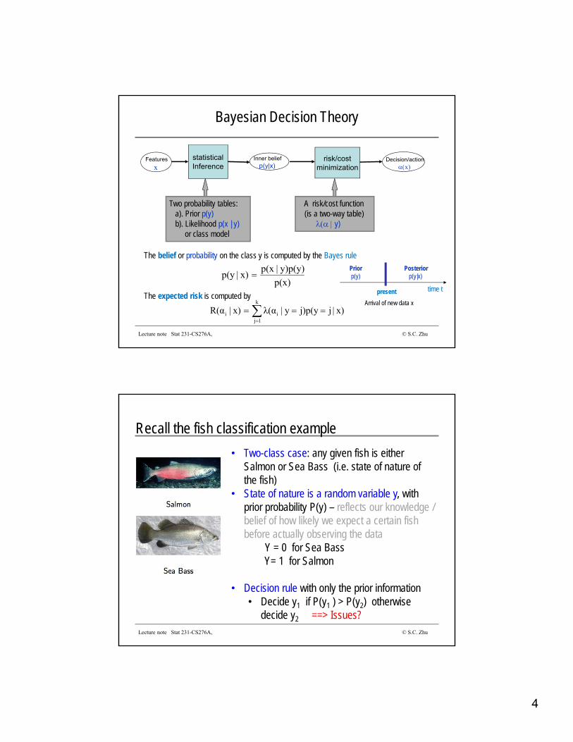
Bayesian Decision Theory

Features

xDecision/action

xInner belief

p(y|x)statisticalInference

risk/costminimization

Two probability tables: a). Prior p(y)b). Likelihood p(x | y)

or class model

A risk/cost function(is a two-way table)

y)

The belief or probability on the class y is computed by the Bayes rule

The expected risk is computed by

p(x)

y)p(y)|p(xx)|p(y

k

1jii x)|jj)p(yy|λ(αx)|R(α

time tpresent

Arrival of new data x

Priorp(y)

Posteriorp(y|x)


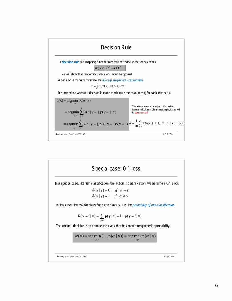
Recall the fish classification example


• Two-class case: any given fish is either Salmon or Sea Bass (i.e. state of nature of the fish)

• State of nature is a random variable y, with prior probability P(y) – reflects our knowledge / belief of how likely we expect a certain fish before actually observing the data

Y = 0 for Sea BassY= 1 for Salmon

• Decision rule with only the prior information• Decide y1 if P(y1 ) > P(y2) otherwise

decide y2 ==> Issues?

5

Illustration of Bayes Rule


lightness

P(x|y)

y1

y2

P(y|x)y1

y2

P(y1) = 2/3

P(y2) = 1/3

p(x)

y)p(y)|p(xx)|p(y

A simple example


Suppose you are betting on which side a tossed coin will fall on. You win $1 if you are right and lose $1 if you are wrong.Let x be whatever evidence that we observe. Together with some prior information about the coin, you believe the head has a 60% chance and tail 40%.

y) |(x)( T}, {H, T}, {H, y y

-1, +1+1, -1

k

1jii x)|jj)p(yy|λ(αx)|R(α

y

=

y

=

0.60.4

-0.20.2

-1, +1+1, -1

So, to minimize the risk, we choose head = H.

and y are shown as indices to the rows/columns of the matrix.

Here risk= -1 means reward 1.

A real example: Bet on presidential elections.

6

Decision Rule

A decision is made to minimize the average (expected) cost (or risk),

It is minimized when our decision is made to minimize the cost (or risk) for each instance x.

dx)()|)(( xpxxRR

d:)(x

j)j)p(yy|j)p(xy|λ(αargmin　　＝

x)|jj)p(yy|λ(αargmin　　　

x)|R(αargminα(x)

k

1jΩ

k

1jΩ

Ω

α

α

α

A decision rule is a mapping function from feature space to the set of actions

we will show that randomized decisions won’t be optimal.


** When we replace the expectation by the average risk of a set of training sample, it is calledthe empirical risk

p(x)~}with_{x_,)x|)R(α(αm

1ˆi

m

1iii

R

Special case: 0-1 loss

In a special case, like fish classification, the action is classification, we assume a 0/1 error.

yify

yify

1)|(

0)|(

)x|(p1)x|p()x|(y

iyyiRi

In this case, the risk for classifying x to class i is the probability of mis-classification

The optimal decision is to choose the class that has maximum posterior probability.

)x|(pmaxarg))x|(p1(minarg)x(


7

Discriminant functions

To summarize, we take an action to maximize some discriminant functions:

x)|iR(α(x)g

i)p(y logi)y|p(x log(x)g

i)i)p(yy|p(x(x)g

x)|ip(y(x)g

i

i

i

i

}{ (x)g...,...(x),g(x),gargmaxα(x) k21


i.e. Bayes or minimum conditional risk discriminant

Discriminant functions

Discriminant functions as network


e.g., x can be raw data instead of selected features and we can stack multiple layers == deep learning

8

Two-class Discriminants

Consider a single discriminant function


A simple rule: decide y1 if g(x) > 0 otherwise decide y2

e.g.,

Partition of feature space

d:)(x

The decision is a partition or coloring of the feature space into k subspaces.

ji,jiik

1i

1 4

35

2

The decision boundaries between two classes i and j are decided by the equation.

ji (x)g (x)g ji


9

Discussion: other decision rule

With 0-1 loss function, the Bayes decision chooses the class with highest posterior probability.

)x|(pmaxarg))x|(p1(minarg)x( Bayes


The Bayes decision is said to yield the minimum error among all possible decision rules.

Discussion:1, What are the assumptions of the conclusion above?

2, One may argue for a randomized decision, will it lead to better results?

)x|(p ~ )x( Random

The decision will be proportional to the probability.

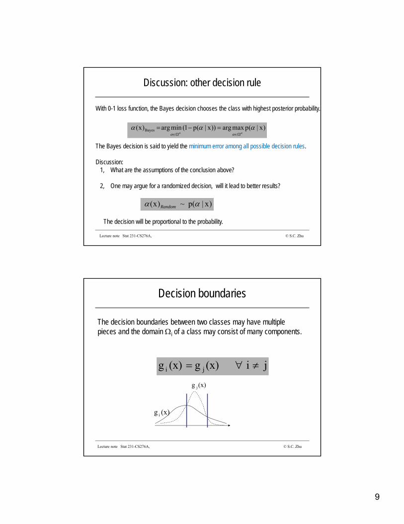
Decision boundaries

(x)g i

(x)g j

The decision boundaries between two classes may have multiple pieces and the domain i of a class may consist of many components.

ji (x)g (x)g ji


10

Decision/classification Boundaries


Decision boundaries for the fish classification example: The left boundary has zero training error – that is often a desirable goal in machine learning.

but it is too specific to the data, and is often said to be “over-fitting”. If we draw a different sample from the data, the boundary will be very different. Such boundary leads to highererror on testing data.

Example: analytic solution of the decision boundary

For simplicity, people often assume Gaussian probabilities for the class models.

We consider a case when

Then the discriminant function is

The boundary equation is a straight line --- linear discriminant or linear machine


11

Close-form solutions

In two case classification, k=2, with p(x|w) being Normal densities, the decision boundaries can be computed in close-form.



Other cases:

12

Discussion of advanced issues

1. “Subjectivism” of the prior in Bayesian decisionSome people may accept that risk/cost can affect the decision boundary, but don’t likethe fact that the prior probability (i.e. the population or frequency of a certain class)affect the decision boundary, as is shown in the figure below.

This means that the Bayesian decision on a certain input “x” is not entirely based on xindividually, but also accounts for the sub-population of the class collectively.So Bayesian decision is a “stereotypical” decision to minimize overall risk/cost, and doing so may cause higher rate of mis-classification to some individuals. Civil rights prevent us from using certain features (such as gender, race) in computing risk or

taking actions, though doing so may be more cost effective.


+ -

x

* Here is an example that the prior probability about the negative populationshifts the decision boundary.

**This is potentially a problem with Deep Learningin blackbox model: How does it remove certain features or bias?


This will choose different features which are most discriminative.

How many examples are enough for learning a model/concept? --- learnability i.e. the probably and approximately correct (PAC)-learning.

2: Learning the probabilities p(y), p(x|y) or p(y|x) --- the subject of machine learning

There are two important factors to consider:

(i) Generative vs. discriminative: which is more effective? This depends on the structures of the feature space and the size of data available.

(ii) Should we learn the probability or just the probability ratio?

)|1(

)|1(

xyp

xyp


13


3, Context or sequential information in classification.

So far, the classification is based on individual input x based on a given model (which is assumed to be learned off-line). In general, one only have very scarce data, therefore we need to consider

(i) Recursive learning and online adaptation of the model

---- This is particularly useful for object tracking.

(ii) Active learning and Markov decision processexploring new features based on current results.



A demo example of sequential learning and tracking

14

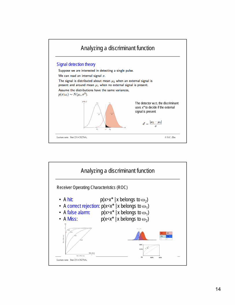
Analyzing a discriminant function


Signal detection theory

The detector w.r.t. the discriminant uses x* to decide if the external signal is present

Analyzing a discriminant function


Receiver Operating Characteristics (ROC)

• A hit: p(x>x* | x belongs to 2)• A correct rejection: p(x<x* | x belongs to 1)• A false alarm: p(x>x* | x belongs to 1)• A Miss: p(x<x* | x belongs to 2)

15

Review of Key Concepts Discussed in Lectures

Paradigm shift by Machine Learning, DNN from traditional statistics

• What is a pattern? • The increasing complexity of: Classification, Recognition, and Understanding • What is a “Machine” and what is “Learning” ?• What is an informative feature, is it to Design, Selection, and Learning features?• When is a feature said to be informative and actionable?• The issue of data dimension in pattern classification: reduction vs expansion?• What is a probability: a frequency vs a belief?• What is a “task”? reflected by loss functions designed to evaluate performance in the task.

• A model or machine is decided by both data and tasks. Deep Neural Network has found its success in a new regime, which is what I called

“Big-Data for Small-Task”. What works here may not be working for your problem in research. For example, in general intelligence, we are facing an opposite regime:

“Small-Data for Big-Task.”

Some popular methods over the years

Documents

Transcript of Some popular methods over the years