"Some New Results on the Estimation of Structural Budget Balance for Spain"; Guido Zack, Pilar...

Some New Results on the Estimation of Structural Budget

Balance for Spain

GUIDO ZACK*

Alcalá University

PILAR POnCELA**

Universidad Autónoma de Madrid

EvA SEnRA

Alcalá University

DAnIEL SOTELSEK***

Alcalá University

Received: April, 2014

Accepted: July, 2014

Summary

The recession that started in 2008 caused a sharp deterioration of the budget balance of Spain. This de-cline was not fully anticipated by the structural budget balance due to some methodology limitations.In this article, we calculate an alternative structural balance for Spain in the years prior to the subprimecrisis that includes residential investment as an explanatory variable. This estimate shows that by 2004the Spanish fiscal situation was not as strong as presumed. This fragility was hidden by the extraordi-nary revenue from the real estate bubble and the construction boom.

Keywords: Crisis, structural budget balance, real estate bubble, construction boom, Spain.

JEL Classification: C20, E32, E63, H62.

1. Introduction

Until 2006 Spain seemed to have one of the most countercyclical fiscal policies in Eu-

rope. In fact, the observed budget balance (OBB) improved from a deficit of 6.5% of GDP in

1995 to a surplus of 2% in 2006. nevertheless, the crisis revealed the fragility of this improve-

ment, since between 2007 and 2009 the OBB fell by 13 percentage points (p.p.) of GDP.

* Guido Zack acknowledges the support of the Institute of Latin American Studies (IELAT), Alcalá Universtity.** Pilar Poncela acknowledges financial support from the Spanish government, Ministerio de Economía y Compet-

itividad, contract grant ECO2012–32854.*** Daniel Sotelsek acknowledges the support of SIPA-ILAS (Columbia University), during his 2013–2014 visit-

ing scholar.

Hacienda Pública Española / Review of Public Economics, 210-(3/2014): 11-31

© 2014, Instituto de Estudios Fiscales

DOI: 10.7866/HPE-RPE.14.3.1

This strong fall is also shown in the structural budget balance (SBB), however neither

the consolidation until 2006 nor the deterioration between 2007 and 2009 can be explained

only by discretionary measures. Situations like that not only happened in Spain, but they

have been occurring in several countries (Larch and Turrini, 2009). Thus, since 2000 there

are several proposals to improve the SBB.

The main objective of this paper is to adapt some of these proposals to the Spanish case

in the years prior to the subprime crisis. In particular, the fiscal impact of the real estate bub-

ble and the boom in the construction industry are incorporated, showing that the SBB is not

capable to identify completely the cycle effect on the budget balance. The improvement of

the SBB methodology is essential in Spain, given that its new budgetary stability law is

based on this indicator.

The article is structured as follows. Section 2 describes the evolution of the Spanish

budget within the European context, identifying a particularly volatile observed and struc-

tural budget balanced trend. This would have been a reflection of the volatile evolution of

residential investment. The SBB was not able to identify the transitory component of the rev-

enue and expenditure. Consequently, in the third section, several improvements of the SBB

traditional methodology proposed by the literature are reviewed. The fourth section adapts

some of these improvements to the particular case of Spain and shows the results obtained.

Finally, conclusions and policy recommendations are presented in section 5.

2. Descriptive analysis of the case of Spain within the European context

2.1. Evolution of public accounts

During the 90s, the budgetary policy in Eurozone countries was dominated by compli-

ance with the Stability and Growth Pact, which established limits on both government deficit

and public debt (3% and 60% of GDP, respectively). In this context, Spain seemed to pio-

neer a counter-cyclical policy. As shown in figure 1, the country progressed from a chroni-

cally high fiscal deficit in the first half of the 90s to a moderate deficit by the end of the

decade, and finally achieved a surplus of 2% of GDP in the years leading up to the reces-

sion. nevertheless, Spanish apparent solvency disappeared with the subprime crisis. Al-

though the recession punished the budgets of all European countries, Spain was particularly

affected. Indeed, between 2007 and 2009 the balance fell from a surplus of 1.9% of GDP to

a deficit of 11.1%, a decline of 13 p.p. in just two years, when the European Union average

(15 countries) fell only by 6 p.p.

Spanish fiscal decline was the result of the evolution of both expenditure and revenue.

The weight of expenditure in the GDP increased by 7 p.p. due to the combined effect of dis-

cretionary policies aimed at maintaining aggregate demand and automatic stabilisers in the

form of unemployment benefits. Revenue, meanwhile, fell by 6 p.p. of GDP, from slightly

more than 41% in 2007 to less than 35% in 2009, the lowest of all Eurozone countries. As

12 GUIDO ZACK, PILAR POnCELA, EvA SEnRA y DAnIEL SOTELSEK

13Some new Results on the Estimation of Structural Budget Balance for Spain

Figure 1. Observed and structural budget balance(as a % of GDP and potential GDP)

Source: European Commission.

shown figure 2, the main reason for this was the loss of revenue from corporate tax (2.4 p.p.),

added value tax (2.3 p.p.), personal income tax (0.9 p.p.) and capital transfer tax and stamp

duty (0.9 p.p.).

The evolution of Spanish SBB in these years did not differ substantially from the OBB.

Indeed, from the mid-90s the SBB also showed a process of fiscal consolidation, reaching a

surplus of 1% of potential GDP in 2006 1. When the subprime crisis hit the market, the SBB

returned to negative figures, with a deficit of 8.6% of potential GDP in 2009 (figure 1).

This shortfall in the Spanish SBB was not seen in other European countries. Thus, it is

essential to ascertain what was different in Spain, moreover considering that its new budg-

etary stability law included in the Spanish Constitution is based on this indicator 2. The an-

swer can be found in the collapse of residential investment, since most revenues were direct-

ly and indirectly linked to the construction industry, while this sector was mainly responsible

for the loss of employment and, therefore, the increase in related expenditure (REAF, 2007).

2.2. Evolution of residential investment

In the years leading up to the 2007 crisis, housing prices rose sharply across most Euro-

pean countries, particularly in the UK and Spain, where they increased threefold, and to a

lesser extent in other countries such as France, Italy and Portugal (figure 3). Although price

variations in Spain were among the greatest, this would not seem enough to explain the no-

table difference in public accounts.

The greatest difference is found in the number of units built: while the GDP share of res-

idential investment remained either steady or even declined in most EU countries, in Spain

it rose sharply until 2006 (figure 4). This is because the increase in housing prices, instead

of discouraging buyers fearful of a reversal of the trend, had the opposite effect based on the

belief that prices would continue to raise, a clear indication of the creation of a bubble 3 (Gar-

cía Montalvo, 2003).


Figure 2. Spanish government revenue and expenditure(as a % of GDP)

Source: Spanish Ministry of the Finance and Public Administrations.

Accordingly, residential investment in Spain grew at an average rate of 8% per year

in real terms over the 1998-2007 period, twice the rate of the economy as a whole and

accounting for one fifth of the rise in GDP. Thus, by 2006 it accounted for 12.5% of

nominal GDP in Spain, when historically it had stood between 5% and 8%. In the

labour market, the construction sector accounted for 13.5% of all jobs in Spain, and

nearly a quarter of the growth in employment over the same period. When the bubble

burst, residential investment shrank to 4.4% of nominal GDP in 2013, while the con-

struction sector was directly responsible for the loss of 60% of the jobs between 2007

and 2011.

To sum up, the evolution of the construction sector and the housing market, not only in

terms of prices but also in the number of units built, could be responsible for the volatility

of Spanish public accounts.


Figure 3. Housing prices in Europe(1996=100)

Source: European Central Bank.

3. SBB traditional methodology limitations

The SBB is estimated by the European Commission (EC) and the International Mone-

tary Fund (IMF). Both organisations base their calculation on the cyclical position of the

economy, i.e., the output gap (OG), and on the relationship between the cycle and the differ-

ent balance components (revenue and expenditure) 4. The cycle is linked to the budget

through the elasticities between the main revenue items (direct taxation of individuals and

companies, indirect taxes and social security contributions) and the OG, while in terms of

expenditure, only unemployment expenditures are considered cyclical. Then, the structural

components are calculated by multiplying the observed revenue or expenditure net of one-

off and temporary measures (Mourre et al., 2013) by the OG to the corresponding elasticity

power. In the case of expenditure, the IMF approach differs from the EC in that instead of

basing their calculations on the OG and the elasticity, they use a simple proportional rule be-

tween observed unemployment expenditures, the rate of unemployment and the non-Accel-

erating Wage Rate of Unemployment (nAWRU). Finally, the structural revenue and expen-


Figure 4. Residential investment in Europe(as a % of GDP, 2005 prices)

Source: European Commission.

diture are subtracted and the result is divided by the potential GDP (Girouard and André,

2005; Hagemann, 1999).

The objective of estimating the SBB is twofold: first, to assess the cyclical behaviour of

discretionary fiscal policies; and second, to attempt to measure the sustainability of such

policies by showing whether a fiscal balance is the result of the cyclical components of rev-

enue and expenditure, or whether it is based on a more stable trend (Blanchard, 1990). nev-

ertheless, in several cases, this indicator failed to explain both, the cyclicality and the sus-

tainability of fiscal policy. The reasons that led to these problems are the following.

First of all, SBB real-time estimation could be biased not because an error in its method-

ology, but because a bias in the OG real-time estimation. Kempkes (2012) shows that the OG

real-time estimation is biased. This bias points towards a more negative OG between 0.5%

and 0.6% of potential output. Thus, if a fiscal rule is based on this indicator, the real-time

admissible deficit will exceed the final value by about 0.5 percentage points per year 5.

Assuming an unbiased OG, SBB could still be biased because of the decoupling between

the tax base and GDP (Kremer et al., 2006; European Commission, 2013, Part III). This can

be partially corrected by taking into account the effects of the composition of demand

through more disaggregated indicators than the OG, such as the tax bases (European Com-

mission, 2007, Part II). But, each tax has sometimes several bases and it is not always pos-

sible to consider all of them. Thus, it is desirable to take into consideration at least the most

important ones and the assets that can be affected by a bubble. If not, a significant bias in

elasticity estimations could be generated 6.

In fact, de Castro et al. (2008) show that output elasticities of revenues and expenditures

are not constant across the cycle, but rather pro-cyclical. This could cause the cyclical pat-

tern in the revenues windfalls and shortfalls (Morris et al., 2009). That is why, in times of

economic growth, part of the cyclical revenue is usually considered structural (Girouard and

Price, 2004; Joumard and André, 2008). Therefore, based on real time data, fiscal policies

seem to be counter-cyclical, while after-the-event input suggests pro-cyclicality (Cimadomo,

2008; Golinelli and Momigliano, 2007; Forni and Momigliano, 2004).

Taking into account the SBB limitations to measure the fiscal policy cyclicality, the Eu-

ropean Commission (2013, part III) has developed a new indicator to measure the discre-

tionary fiscal effort (DFE). It consists of a narrative (bottom-up) approach on the revenue

side and a traditional (top-down) approach on the expenditure side. A comparison of both in-

dicators shows that, during booms, DFE indicates a more pro-cyclical policy than real time

estimation of SBB, in line with the evidence presented in the previous paragraph.

However, the DFE does not aim at measuring the sustainability of the fiscal policy. To

do so, and taking into account the SBB limitations reviewed in this section, the impact of

bubbles and booms in the cyclical components needs to be considered. In fact, de Castro et

al. (2008) and Morris et al. (2009) recognize that the housing boom could be responsible for


the notable revenues windfalls presented in Spain between 1999 and 2007. So, this paper

main objective is to include the real estate asset in the Spanish SBB estimation during the

years prior to the subprime crisis at the aim of improving the fiscal policy sustainability

measure.

4. Estimated structural budget balance for Spain

4.1. Methodology

First of all, tax collection must be disaggregated into revenue categories. As we are deal-

ing specifically with Spain, we can achieve a more accurate disaggregation instead of rely-

ing on the EC general categories. Revenue is therefore disaggregated into: social security

contributions (SSC), personal income tax (PIT), corporate tax (CT), property tax (PT; in-

cludes inheritance and gift tax and the discontinued wealth tax), value added tax (vAT), cap-

ital transfer tax and stamp duty (CTT-SD) and regional governments revenue (RG) 7.

Tax base proxies are used instead of the OG as explanatory variables. Thus composition

effects are considered. The tax base proxies used for each revenue item are as follows: for

the SSC, the average wage (W), the number of people employed (EM), and unemployment

benefits (UB); for PIT, the gross disposable household income (GDHI) and the average tax

rate (RatePIT); for CT, the gross disposable corporate income (GDCI) and the average tax

rate (RateCT) 8; for vAT, private consumption (PRC). Finally, for the PT, the CTT-SD and

the RG the residential investment (RI) is the only explanatory variable. RI is also included

in all the equations as an additional tax base because it takes into accounts not only prices,

but also quantities. Therefore, it can be considered as a proxy of economy-wide effects, since

the number of units built may affect employment in the construction sector, wage increases

and consumption rises, among others.

Annual data from 1986 to 2010 are used and the sources can be found at the annex A.

Following Girouard and Price (2004), Kremer et al. (2006), Morris and Schuknecht

(2007), and Price and Dang (2011), an error correction model was estimated for each tax rev-

enue category to capture both, short- and long-term relationships. Accordingly, we have es-

timated a long-term equation (1) linking the levels of the variables (in logarithms) for each

revenue category. Equation (2) shows the short-term dynamics between the revenue varia-

tion rate, due to long-term deviations from equilibrium, the variation rate of the respective

tax base proxies and (nominal) residential investment.

(1)

(2)

ln ln ln, , , ,T B RIi t i i jj

N

i j t i tlt lt

i

lt= + + +

=∑α β γ1

εεi t,

∆ = + ∆ + ∆=

∑ln ln ln, , , ,

T B Ri t i i jj

N

i j t ist st

i

stα β γ

1

II et i i t i t+ +−δ ε, ,1


where Tiis the observed revenue of the “i” revenue category; B

i,jis the “j” tax base proxy of

the “i” revenue category; Rl is the nominal residential investment; bi,j

is the elasticity 9 of “i”

revenue to the “j” tax base; giis the elasticity of the “i” revenue items to nominal residential

investment; subscripts “lt” and “st” stand for the long-term and short-term equations respec-

tively; diis the error correction factor; ∆ is the first difference operator; and ln is the natural

logarithm.

Once the coefficients have been obtained, the equation yields the structural value of each

revenue item based on the long-term values of the tax bases and residential investment prox-

ies. In the former case, following Kremer et al. (2006), tax bases proxies were smoothed

using a Hodrick – Prescott filter (λ=30) 10. In the latter case, the long-term value is taken to

be a fixed percentage of nominal GDP. various scenarios are developed based on the evo-

lution over time in Spain, ranging from 5% to 8% 11. Therefore, the structural value of each

revenue item is obtained from the following equation, adapted from the EC and IMF

methodology based on the OG (Girouard and André, 2005; Hagemann, 1999):

(3)

where the superscript “*” indicates structural value.

Adding up all structural revenue and tax revenue not included in the quantitative calcu-

lation (basically excise tax, foreign trade and gambling tax, that represent less than 10% of

total revenue and are taken to be unrelated to the evolution of the construction industry), we

obtain the total structural revenue.

(4)

where the superscript “*” indicates structural value; T is the total revenue; Tiis the revenue

stemming from residential investment; and NIT are the revenue items not related to residen-

tial investment.

According to the EC and IMF approaches, the only cyclical item of expenditure is un-

employment benefits (Girouard and André, 2005; Hagemann, 1999). The nAWRU, estimat-

ed by the EC, is used as the structural unemployed rate. However, the methodology of this

indicator (Mc Morrow and Roeger, 2000) affirms that it cannot be considered structural,

since it estimates the unemployment rate that stabilises the inflation rate, while the long-term

rate should stabilise both inflation and unemployment. Consequently our methodology does

not use the annual nAWRU value, but rather its 20-year moving average 12. This increases

the unemployment expenditure that is considered cyclical because it allows a greater differ-

ence between the long-term and observed unemployment rate. For the sake of simplicity, we

have followed the IMF method of calculating cyclical expenditure, i.e., a proportional rule

considering the monetary value of unemployment benefits, divided by the unemployment

rate and multiplied by the nAWRU moving average.

T TB

B

RI

RIi ii j

i jj

Nii jlt

* ,

*

,

*,

=

=∏1

β

γ ilt

T T NITi* *= +∑


(5)

where the superscript “*” indicates the structural value; E is the total public expenditure; Ec

is the cyclical public expenditure; Eu

is the unemployment expenditure; and UR is the unem-

ployment rate.

Finally, SBB is obtained by subtracting revenue from structural expenditures.

SBB* = T* – E* (6)

4.4. Results

First of all, we perform Dickey-Fuller (1981) unit roots tests to identify the order of in-

tegration of all variables. As shown in table B.1 in the annex B, we did not reject the unit

root hypothesis for the levels of the variables (in logarithms) in any case.

Table 1 shows short- and long-term coefficients obtained from the error correction

model estimated on each tax revenue using as covariates their tax base and nominal residen-

tial investment proxies, together with the error correction term. The annex B shows evidence

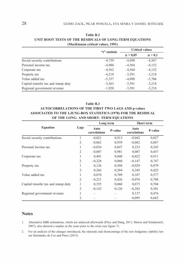
that confirms the suitability of the models used. Specifically, table B.2 shows the statistics

of the unit root test on the residuals of the long-term equations and MacKinnon’s (1991) crit-

ical values. It can be seen that, with the exception of the RG variable, the unit root null hy-

potheses is rejected for the residuals of all long-term equations (1), and as such they can be

considered stationary. In the case of RG, we concluded that there is no cointegration rela-

tionship between this variable and residential investment. Table B.3 shows the autocorrela-

tion value of the first two lags of the residuals from the long-term equations (1) and the error

correction models (2). The Ljung-Box (1978) statistic shows that the residuals in all short-

term equations are white noise, which confirms the suitability of the models. The residuals

of the long-term equations or cointegration relationships can be considered white noise for

all variables, except for IS. In this case, the efficiency of the cointegration vector estimation

can be improved using Stock and Watson’s (1993) dynamic ordinary least squares (DOLS)

technique, that shows very similar results 13.

Going back to table 1, it can be seen that residential investment turned out to be a very

significant variable to explain the evolution of all the revenue items considered, and that the

coefficients signs are as expected. Likewise, the remaining variables are also significant, and

their signs as expected too 14. Error correction terms, which show the percentage of devia-

tion corrected for each period, are significant, being in all cases between 39% and 87%, ex-

cept for SSC, which seems to over-correct the deviation by 9%.

It can also be seen that there are no RG values in either the long-term equation or the

error correction term. This is because, as discussed previously, the residuals from its long-

E E E E E E E E EUR

URE Ec u u u u u

* **

( )= − = − − = − −

= − 1−−

UR

UR

*


term equation were not stationary. Therefore, in this case, we supposed that there is no coin-

tegration relationship between variables, meaning that the coefficient used to estimate

structural revenue is taken from the short-term equation in which no error correction was

included.

Table 1

TAX REVENUE ELASTICITIES

Error

RI W EM UB GDHI RatePIT GDCI RateCT PRC C correction R2

term

Short-term

SSC 0.15** 0.82*** 0.59** 0.07** 0 –1.09*** 0,90

–0,06 –0,1 –0,22 –0,03 –0,01 –0,26

PIT 0.20*** 0.43*** 0.18*** 0.03*** –0.69*** 0,98

–0,03 –0,14 –0,01 –0,01 –0,2

CT 0.39*** 0.42** 0.33*** 0 –0.39** 0,92

–0,08 –0,12 –0,03 –0,01 –0,15

PT 0.99*** 0 –0.87*** 0,58

–0,25 –0,04 –0,21

vAT 0.73*** 1.58*** –0.11*** –0.89*** 0,99

–0,13 –0,45 –0,02 –0,16

CTT–SD 1.39*** 0 –0.82*** 0,66

–0,19 –0,03 –0,21

RG 0.29*** 0.06*** – 0,47

–0,06 –0,02 –

Long–term

SSC 0.13*** 0.87*** 0.61*** 0.08*** 0,16 0,99

–0,04 –0,04 –0,16 –0,02 –0,85

PIT 0.14*** 0.90*** 0.14*** –3.62*** 0,99

–0,02 –0,04 –0,01 –0,32

CT 0.28** 0.65*** 0.38*** –1,30 0,98

–0,12 –0,15 –0,05 –1,00

PT 0.85*** –0,38 0,93

–0,05 –0,86

vAT 0.46*** 0.33*** 0,00 0,99

–0,04 –0,04 –3,95

CTT–SD 1.05*** –2.98*** 0,97

–0,04 –0,65

note: *** significant at 1%; ** significant at 5%; * significant at 10%.

Figures 5 and 6 show the evolution of total revenue and unemployment expenditure, re-

spectively, both in terms of observed and structural values. In the case of revenue, different

long-term residential investment scenarios are presented. It can be seen that up to 2002 the

observed revenue did not differ significantly from the structural revenue as expected. How-

ever, from 2002 to 2008 the observed revenue exceeded all long-term residential investment

scenarios, peaking in 2007 with a difference of 3.3% of GDP compared with the average sce-

nario (6.5%). Since 2009, after the bubble burst, the observed value has returned to the struc-

tural one.


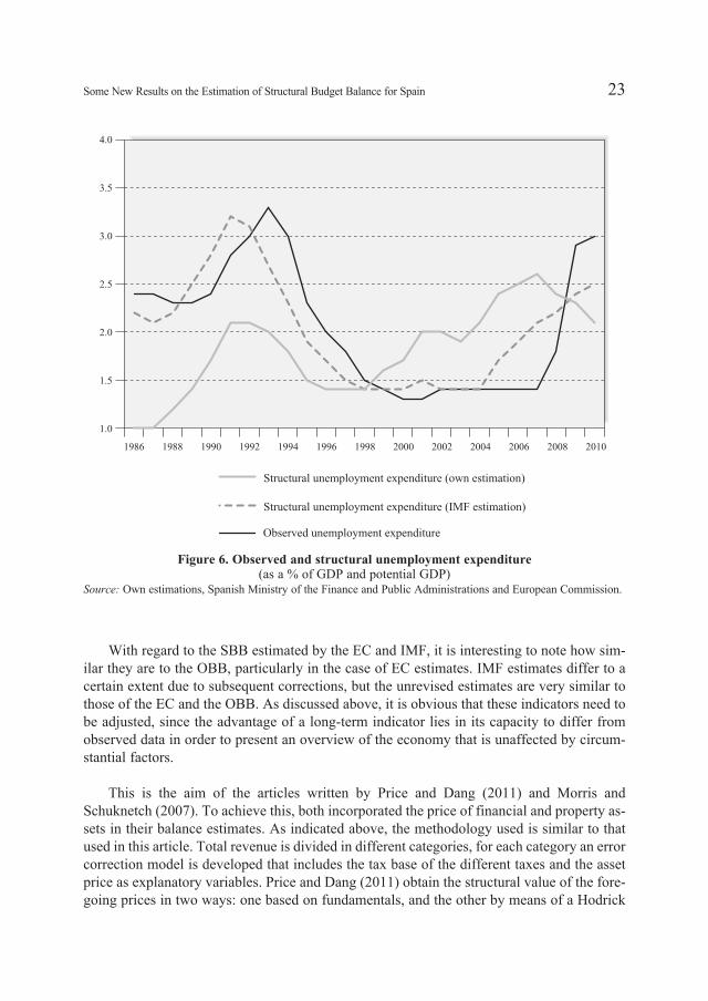
Regarding unemployment expenditures, the observed and the traditional structural ones

are very close to each other, given the small difference between the unemployment rate and

the nAWRU. On the contrary, our structural estimation presents lower values until 1998 and

higher values from that year on. The highest difference in comparison with the observed

value is 1.1% of GDP in 2006 and 2007. Since 2009, our estimation is lower again, given

that it does not take into account completely the extremely high unemployment rate of these

years and due to the reduction in the unitary benefits.

Finally, figure 7 shows the OBB, the SBB estimated by the EC and IMF, our own esti-

mate of the SBB for the average scenario (where the nominal GDP share of residential in-

vestment is 6.5%) and other estimates from earlier papers (Price and Dang, 2011; Morris and

Schuknetch, 2007). First, it can be seen that all the SBB are relatively similar until 1998.

From this year onwards, our own estimate starts to show a downward trend that dips more

sharply after 2001, while the remaining estimations maintain their upward trend for several

more years.


Figure 5. Observed and structural revenue(as a % of GDP and potential GDP)

Source: Own estimations and Spanish Ministry of the Finance and Public Administrations.

With regard to the SBB estimated by the EC and IMF, it is interesting to note how sim-

ilar they are to the OBB, particularly in the case of EC estimates. IMF estimates differ to a

certain extent due to subsequent corrections, but the unrevised estimates are very similar to

those of the EC and the OBB. As discussed above, it is obvious that these indicators need to

be adjusted, since the advantage of a long-term indicator lies in its capacity to differ from

observed data in order to present an overview of the economy that is unaffected by circum-

stantial factors.

This is the aim of the articles written by Price and Dang (2011) and Morris and

Schuknetch (2007). To achieve this, both incorporated the price of financial and property as-

sets in their balance estimates. As indicated above, the methodology used is similar to that

used in this article. Total revenue is divided in different categories, for each category an error

correction model is developed that includes the tax base of the different taxes and the asset

price as explanatory variables. Price and Dang (2011) obtain the structural value of the fore-

going prices in two ways: one based on fundamentals, and the other by means of a Hodrick


Figure 6. Observed and structural unemployment expenditure(as a % of GDP and potential GDP)

Source: Own estimations, Spanish Ministry of the Finance and Public Administrations and European Commission.

and Prescott filter. Morris and Schuknetch (2007) only use the filter. Despite these changes,

it is interesting to note that their structural estimates do not differ to any great extent; at least

they are not capable of identifying fiscal difficulties in advance of observed balances.

The main advantage of the approach suggested here, therefore, is that it shows that long-

term public accounts had started to deteriorate in 1999, with a 3% potential GDP deficit by

2002, and below 4% from 2004 onwards. This would have identified Spanish potential fis-

cal troubles several years in advance, and measures could have been taken to correct them

in real time. The estimation is improved because the general methodology for all countries

is adapted to a particular case. The main feature of Spain over the period studied, as dis-

cussed above, is that the real estate bubble was accompanied by a construction boom, which

means that the process not only affected prices but also the number of units built, a factor

that was not taken into consideration in earlier papers. In other words, instead of discourag-

ing buyers, the rise in housing prices had the opposite effect due to the belief that the upward

trend would continue. This is why it was decided to include nominal residential investment

in our SBB calculation in order to capture the effect of both the prices and units built.


Figure 7. Observed and structural budget balance(as a % of GDP and potential GDP, respectively)

Source: Own estimations, Spanish Ministry of the Finance and Public Administrations, EC, IMF and referred papers.

As a robustness check, we have estimated our model with data up to 2004 and 2007. We

obtain similar results and none of our conclusions are altered 15. The scenario after the crisis

may have changed. We were able to estimate a model with data up to 2004 and 2007 because

we had enough data. Unfortunately, we only have few observations after the crisis and it is

not possible to estimate a model with these few data. But, in any case, the current SBB esti-

mation is not the final word on the future outlook for public finances in Spain. In fact, the

lower growth rates that are foreseen for Spain in the next years should be taken into account

in future research.

5. Conclusions

This article attempts to make a contribution to understand the extremely deterioration in

the Spanish budget balance. This situation could not be anticipated by the SBB estimated by

the EC and the IMF, given that they showed a structural surplus until 2007. Based on these

figures, the Spanish authorities took a series of decisions to fight against the recession of

2008 on the assumption that public accounts were structurally sound and had a large enough

buffer to allow counter-cyclical policies to be implemented. However, it later became evi-

dent that the buffer was nowhere near as robust as expected, forcing them to withdraw tax

incentives before the private sector was ready to spearhead the aggregate demand.

Such situations might arise due to the failure to include the effect of bubbles in SBB cal-

culations. nevertheless, estimates carried out by other authors who did include such vari-

ables in their calculations were not capable of improved significantly Spanish SBB either, at

least not enough to identify the deterioration of the fiscal situation in time. The main reason

for this is that the studies were carried out for a group of countries or a particular region, and

as such the particular characteristics of each country are not factored in.

In this regard, Spain was in a unique situation because the real estate bubble affected not

only prices but also the number of units built, which means that including property prices as

the sole explanatory variable of tax revenue was not enough. In this article we have used

nominal residential investment as a way of including the number of units built too. It is in-

teresting to note that this type of investment has, historically, represented around 6.5% of

nominal GDP, but it reached 12.5% in the years leading up to the crisis.

The results obtained confirm how important residential investment was in Spanish tax

revenue, at least, until the bubble burst. Indeed, it can be seen that including this variable in

the equation, and assuming different scenarios concerning its long-term share in GDP, re-

veals that Spanish SBB started to show a strong deficit as far back as 2004. Taken this data

into consideration, different fiscal policy decisions would probably have been taken not only

from 2008 onwards, since the start of the crisis, but also in preceding years.

To conclude, it is essential to include bubbles and booms in SBB estimates. This is es-

pecially important in Spain, given that its fiscal rule is based on this indicator.



Annex A

Serie Source

Observed budget balance

Total revenues

Social security contributions

Total expenditures

Unemployment benefits

Gross domestic product

Gross disposable corporate income

Gross disposable household income

Private consumption

Employment

Unemployment

Wages

Personal income tax

Corporate tax

Inheritance and gift tax

Wealth tax

value added tax

Capital transfer tax

Stamp duty

Real Property Tax

Motor vehicle Tax

Urban Land value Increase Tax

Tax on Economic Activities

Tax on Building, Installations and

other Work

Local rates

Structural budget balance

Potential GDP

Structural revenues

Structural expenditures

nAWRU

Residential investment

Housing prices

Average personal income tax rate

Average corporate tax rate

Ministerio de Hacienda y Administraciones Públicas

de España

http://www.sepg.pap.minhap.gob.es/sitios/sepg/es-ES/Presu-

puestos/Documentacion/paginas/bdmacro.aspx


de España

http://www.minhap.gob.es/es-ES/Estadistica%20e%20Infor-

mes/Impuestos/Paginas/Impuestos.aspx


de España

http://serviciosweb.meh.es/apps/EntidadesLocales/

European Commission

http://ec.europa.eu/economy_finance/ameco/user/serie/Se-

lectSerie.cfm

International Monetary Fund

http://www.imf.org/external/ns/cs.aspx?id=28

European Commission

http://ec.europa.eu/economy_finance/ameco/user/serie/Se-

lectSerie.cfm

European Commission

http://epp.eurostat.ec.europa.eu/portal/page/portal/statistics/s

earch_database

European Central Bank

http://sdw.ecb.europa.eu/browse.do?node=2120781

OECD

http://stats.oecd.org/


An

nex

BT

ab

le B

.1

UN

IT R

OO

T T

ES

TS

(D

ick

ey-F

ull

er c

riti

cal

valu

es,

1981)

Lev

els

Fir

st D

iffe

ren

ces

Sec

on

d d

iffe

ren

ces

Va

ria

ble

No i

nte

rcep

t,W

ith

in

terc

ept,

Wit

h i

nte

rcep

t,N

o i

nte

rcep

t,W

ith

in

terc

ept,

No i

nte

rcep

t,n

o t

ren

dn

o t

ren

da

nd

tre

nd

no t

ren

dn

o t

ren

dn

o t

ren

d

“t”

stat

isti

cP

-val

ue

“t”

stat

isti

cP

-val

ue

“t”

stat

isti

cP

-val

ue

“t”

stat

isti

cP

-val

ue

“t”

stat

isti

cP

-val

ue

“t”

stat

isti

cP

-val

ue

Soci

al s

ecur

ity c

ontr

ibut

ions

0,

277

0,75

7 –0

,777

0,

807

–2,5

25

0,31

4 –1

,157

0,

218

–1,8

26

0,35

9 –4

,665

0,

000

Pers

onal

inco

me

tax

3,77

7 1,

000

2,14

4 1,

000

–0,9

67

0,92

5 0,

513

0,81

7 –4

,266

0,

003

– –

Cor

pora

te ta

x –0

,318

0,

560

–1,3

99

0,56

6 –1

,732

0,

697

–3,5

34

0,00

1 –2

,034

0,

271

– –

Prop

erty

tax

–0,2

40

0,58

9 –1

,484

0,

524

–2,8

84

0,18

5 –4

,611

0,

000

–4,5

70

0,00

2 –

–

val

ue a

dded

tax

0,95

8 0,

905

–1,0

11

0,73

2 –2

,850

0,

197

–4,0

01

0,00

0 –4

,008

0,

007

– –

Cap

ital t

rans

fer

tax

and

stam

p du

ty

–0,8

68

0,32

9 –1

,881

0,

335

–0,7

34

0,95

6 –2

,624

0,

011

–3,1

88

0,03

5 –

–

Reg

iona

l gov

ernm

ent r

even

ue

3,94

0 1,

000

3,62

2 1,

000

1,36

6 1,

000

–0,6

84

0,40

8 –2

,041

0,

268

–5,2

65

0,00

0

Res

iden

tial i

nves

tmen

t 3,

340

0,99

9 1,

942

1,00

0 –0

,574

0,

971

–1,3

45

0,16

0 –4

,265

0,

003

– –

Wag

e 1,

165

0,93

2 –1

,045

0,

718

–3,2

09

0,11

4 –0

,701

0,

401

–3,4

93

0,01

8 –

–

Em

ploy

ed

1,58

0 0,

968

–1,3

80

0,57

4 –2

,869

0,

190

–1,7

94

0,07

0 –2

,721

0,

087

– –

Une

mpl

oym

ent b

enef

its

3,12

0 0,

999

2,07

8 1,

000

0,75

5 0,

999

–2,4

70

0,01

6 –2

,798

0,

074

– –

Con

sum

ptio

n 2,

707

0,99

7 2,

058

1,00

0 –2

,031

0,

555

–1,4

19

0,14

1 –3

,246

0,

030

– –

Hou

seho

ld in

com

e 21

,120

1,

000

6,49

1 1,

000

2,65

9 1,

000

–0,9

22

0,30

6 –1

,052

0,

713

–5,9

63

0,00

0

Cor

pora

te in

com

e 3,

339

0,99

9 0,

627

0,98

7 –2

,000

0,

566

–2,1

64

0,03

2 –3

,922

0,

008

– –

PIT

rat

e 0,

534

0,82

4 –1

,694

0,

421

–2,1

58

0,48

9 –6

,263

0,

000

–6,0

74

0,00

0 –

–

CT

rat

e –0

,422

0,

520

–1,7

72

0,38

5 –2

,760

0,

225

–4,0

05

0,00

0 –3

,903

0,

007

– –


Table B.2

UNIT ROOT TESTS OF THE RESIDUALS OF LONG-TERM EQUATIONS

(MacKinnon critical values, 1991)

“t” statisticCritical values

a = 0,05 a = 0,1

Social security contributions –4,759 –4,998 –4,567

Personal income tax –4,980 –4,564 –4,152

Corporate tax –4,562 –4,564 –4,152

Property tax –4,218 –3,591 –3,218

value added tax –5,357 –4,098 –3,706

Capital transfer tax and stamp duty –3,363 –3,591 –3,218

Regional government revenue –1,920 –3,591 –3,218

Table B.3

AUTOCORRELATIONS OF THE FIRST TWO LAGS AND p-values

ASSOCIATED TO THE LJUNG-BOX STATISTICS (1978) FOR THE RESIDUAL

OF THE LONG- AND SHORT- TERM EQUATIONS

Equation Lags

Long term Short term

AutoP-value

AutoP-value

correlations correlations

Social security contributions 1 –0,021 0,913 –0,042 0,827

2 –0,062 0,939 –0,082 0,887

Personal income tax 1 –0,036 0,847 0,223 0,245

2 –0,007 0,981 0,087 0,457

Corporate tax 1 0,401 0,040 –0,022 0,911

2 –0,228 0,060 –0,147 0,747

Property tax 1 0,126 0,504 –0,029 0,879

2 0,266 0,284 0,245 0,422

value added tax 1 0,070 0,709 0,107 0,577

2 –0,231 0,426 –0,076 0,788

Capital transfer tax and stamp duty 1 0,355 0,060 0,073 0,704

2 –0,142 0,126 –0,282 0,301

Regional government revenue 1 – – 0,137 0,476

2 – – –0,095 0,682

Notes

1. Alternative SBB estimations, which are analyzed afterwards (Price and Dang, 2011; Morris and Schuknetch,

2007), also showed a surplus in the years prior to the crisis (see figure 7).

2. For an analysis of the changes introduced, the rationale and shortcomings of the new budgetary stability law

see Hernández de Cos and Pérez (2013).

3. According to Stiglitz (1990) a bubble exists when the price of an asset grows only because investors believe

it will continue to increase in the future, although fundamental factors do not justify this belief.

4. While the OG is an essential driver of the SBB, its estimation remains outside the scope of this paper. For the

OG estimation, see Denis et al. (2006) and D’Auria et al. (2010).

5. This real-time bias in the admissible deficit would be added to another bias identified by de Castro et al.

(2013), related to political issues such as unfavorable economic conditions or elections.

6. For example, if a financial or real estate bubble raises the price of assets, it would affect certain tax bases, but

not the OG, affecting the elasticities (Joumard and André, 2008).

7. This category is the sum of Real Property Tax (Impuesto sobre bienes inmuebles, or “IBI”), Motor vehicle

Tax (Impuesto sobre vehículos tracción mecánica, or “IvTM”), Urban Land value Increase Tax (Impuesto

sobre incremento valor terrenos naturaleza urbana, or “IIvTnU”), Tax on Economic Activities (Impuesto

sobre actividades económicas, or “IAE”), Tax on Building, Installations and other Work (Impuesto sobre con-

strucciones, instalaciones y obras, or “ICIO”), and local rates.

8. RatePIT and RateCT are calculated by the OECD as the ratio between the personal income tax and the corpo-

rate tax revenues, respectably, and the GDP. Therefore, these are not statutory rates.

9. Equations (1) and (2) should take on board legislation changes in order for β and γ to be interpreted as proper

tax elasticities in the sense in which the literature uses them. As we focus on the fit of the equations, we use

these coefficients as proxies of the real elasticities.

10. The choice of the value of the parameter is discussed in Bouthevillain et al. (2001).

11. In the pre-bubble two decades (between 1980 and 2000), residential investment had never been less than 5%

or more than 8% of GDP.

12. Results are not significantly modified when different moving averages are used.

13. Results are available upon request.

14. We attempted to include lagged variables in short-term equations, but none were significant. This was expect-

ed since annual data are used. Thus, only contemporary dynamics are shown.

15. We thank both anonymous referees for suggesting this robustness check.

References

Blanchard, O. J. (1990), “Suggestions for a new set of fiscal indicators”, OECD Department of Eco-

nomics and Statistics Working Papers, 79.

Bouthevillain, C.; Cour-Thimann, P.; van den Dool, G.; Hernández de Cos, P.; Langenus, G.; Mohr,

M.; Momigliano, S. and Tujula, M. (2001), “Cyclically adjusted budget balances: an alternative ap-

proach”, European Central Bank Working Paper Series, 77.

Cimadomo, J. (2008), “Fiscal policy in real time”, European Central Bank Working Paper Series, 919.

D’Auria, F.; Denis, C.; Havik, K.; Mc Morrow, K.; Planas, C.; Raciborski, R.; Röger, W. and Rossi,

A. (2010), “The production function methodology for calculating potential growth rates and output

gaps”, European Commission Economic Papers, 420.

de Castro Fernández, F.; Estrada García, A.; Hernández de Cos, P. and Martí Esteve, F. (2008), “Una

aproximación al componente transitorio del saldo público en España”, Boletín Económico del Banco

de España, 6: 71-81.


de Castro, F.; Pérez, J. and Rodríguez-vives, M. (2013), “Fiscal Data Revisions in Europe”, Journal

of Money, Credit and Banking, 45 (6): 1187-1209.

Denis, C.; Grenouilleau, D.; Mc Morrow, K. and Röger, W. (2006), “Calculating potential growth rates

and output gaps – A revised production function approach”, European Commission Economic Pa-

pers, 247.

Dickey, D. A. and Fuller, W. A. (1981), “Likehood ratio statistics for autoregressive time series with

a unit root”, Econometrica, 49 (4): 1057-1072.

European Commission (2007), “Public finances in EMU 2007”, European Economy, 3.

European Commission (2013), “Report on Public finances in EMU 2013”, European Economy, 4.

Forni, L. and Momigliano, S. (2004), “Cyclical sensitivity of fiscal policies based on real-time data”,

MPRA Paper, 4315.

García Montalvo, J. (2003), “La vivienda en España: desgravaciones, burbujas y otras historias”, Fun-

dación de las Cajas de Ahorro (FUNCAS), Perspectivas del Sistema Financiero, 78.

Girouard, n. and André, C. (2005), “Measuring Cyclically-adjusted Budget Balances for OECD Coun-

tries”, OECD Economics Department Working Papers, 434.

Girouard, n. and Price, R. (2004), “Asset Price Cycles, ´One-Off´ Factors and Structural Budget Bal-

ances”, OECD Economics Department Working Papers, 391.

Golinelli, R. and Momigliano, S. (2007), “The Cyclical Response of Fiscal Policies in the Euro Area -

Why Do Results of Empirical Research Differ so Strongly?”, Banca d`Italia Working Papers, 654.

Hagemann, R. (1999), “The Structural Budget Balance. The IMF´s Methodology”, IMF Working

Paper, 95.

Hernández de Cos, P. and Pérez, J. (2013), “The new budgetary stability law”, Bank of Spain Econom-

ic bulletin, April: 13-25.

Joumard, I. and André, C. (2008), “Revenue Buoyancy and its Fiscal Policy Implications”, OECD Eco-

nomics Department Working Papers, 598.

Kempkes, G. (2012), “Cyclical adjustment in fiscal rules: some evidence on real-time bias for EU-15

countries”, Discussion Paper Deutsche Bundesbank, 15.

Kremer, J.; Rodrigues Braz, C.; Brosens, T.; Langenus, G.; Momigliano, S. and Spolander, M. (2006),

“A Disaggregated Framework for the Analysis of Structural Developments in Public Finances”, Eu-

ropean Central Bank Working Paper Series, 579.

Larch, M. and Turrini, A. (2009), “The cyclically-adjusted budget balance in EU fiscal policy making:

A love at first sight turned into a mature relationship”, European Commission Economic Papers, 374.

Ljung, G. M. and Box, G. E. P. (1978), “On a Measure of a Lack of Fit in Time Series Models”, Bio-

metrika, 65(2): 297-303.

MacKinnon, J. G. (1991), “Critical values for Cointegration Tests”, in R. F. Engel and C. W. I.

Granger (eds.), Long Run Economic Relationship, Oxford University Press, 267-76.

Mc Morrow, K. and Roeger, W. (2000), “Time –varying nairu / nawru Estimates for the EU’s Mem-

ber States”, Economic and Financial Affairs (ECFIN) of the European Commission, 145.


Morris, R. and Schuknecht, L. (2007), “Structural balances and revenue windfalls. The role of asset

prices revisited”, European Central Bank Working Paper Series, 737.

Morris, R.; Rodrigues Braz, C.; de Castro, F.; Jonk, S.; Kremer, J.; Linehan, S.; Marino, M.; Schalck,

C. and Tkacevs, O (2009), “Explaining government revenue windfalls and shortfalls: an analysis for

selected EU countries”, European Central Bank Working Paper Series, 1114.

Mourre, G.; Isbasoiu, G.; Paternoster, D. and Salto, M. (2013), “The cyclically-adjusted budget bal-

ance used in the EU fiscal framework: an update”, European Economy Economic Papers, 478.

Price, R. and Dang, T. (2011), “Adjusting fiscal balances for asset prices cycles”, OECD Economics

Department Working Paper, 868.

REAF (Registro de Economistas Asesores Fiscales) (2007), “Costes asociados a la adquisición, uso y

alquiler de viviendas”. http://www.unionprofesional.com/index.php/unionprofesional/sala_prensa/noti-

cias_colegiales/economia_sociedad/costes_fiscales_asociados_a_la_adquisicion_uso_y_alquiler_de_vi

viendas_segun_un_estudio_del_reaf

Stiglitz, J. (1990), “Symposium on Bubbles”, Journal of Economic Perspectives, 4(2): 13-18.

Stock, J. H. and Watson, M. W. (1993), “A Simple Estimator of Cointegrating vectors in Higher Order

Integrated Systems”, Econometrica, 61(4): 783-820.

Resumen

La recesión iniciada en 2008 generó un fuerte deterioro del resultado fiscal de España. Este deteriorono fue completamente anticipado por el resultado fiscal estructural debido a ciertas limitaciones meto-dológicas. En este artículo se calcula un resultado estructural alternativo para España durante los añosprevios a la crisis subprime, que incluye la inversión en vivienda como variable explicativa. Esta esti-mación muestra que desde 2004 la situación fiscal española no era tan sólida como se creía y que lafragilidad estuvo oculta gracias a los recursos extraordinarios resultantes de la burbuja inmobiliaria ydel boom en la construcción.

Palabras clave: crisis, resultado fiscal estructural, burbuja inmobiliaria, boom de la construcción, Es-paña.

Clasificación JEL: C20, E32, E63, H62.


"Some New Results on the Estimation of Structural Budget Balance for Spain"; Guido Zack, Pilar...

Economy & Finance

Transcript of "Some New Results on the Estimation of Structural Budget Balance for Spain"; Guido Zack, Pilar...