SOME ANALYTIC RESULTS CONCERNING THE MASS SPECTRUMjpac/QCDRef/1980s/SOME ANALYTIC... · SOME...

Nuclear Physics B219 (1983) 233-261 © North-Holland Publishing Company

SOME A N A L Y T I C RESULTS CONCERNING THE MASS SPECTRUM OF Y A N G - M I L L S G A U G E T H E O R I E S ON A T O R U S 1

M. LUSCHER

Institut [iir Theoretisehe Physik, Universitiit Bern, Sidlerstrasse 5, CH-3012 Bern, Switzerland

Received 4 January 1983

When non-abelian gauge fields are enclosed in a box with periodic boundary conditions, the spectrum of the hamiltonian becomes discrete and the energy values can be expanded in a power series of a = g2/3 ( g : renormalized coupling constant). A method to obtain these expansions is explained and worked out to one-loop order. No numbers for the low-lying levels are given here, but some interesting properties of the mass spectrum already become visible.

1. Introduction and summary

In a recent letter [1], I proposed a universal expansion for the masses of the low-lying stable particles in asymptotically free field theories. The method is based

on the observation that the energy spectrum of field theories in a box is discrete

and peturbatively computable. The main difficulty then is, to work out the perturbation expansion of the low-lying levels to a sufficiently high order. This problem is

here attacked for the case of (pure) SU(n) Yang-Mills gauge theories in 3 + 1

dimensions. Gauge theories on a torus were studied by 't Hooft [5]. He noticed that in

addition to the usual symmetries, the hamiltonian commutes with a group of

non-trivial transformations related to the centre Z , of SU(n). They will be described

in detail in sect. 2. Here, I only remark that they give rise to a division of the physical Hilbert space into n 3 orthogonal subspaces, the "central sectors"*, which

have a property characteristic for super selection sectors: application of local

operators to the states in a given sector does not lead out of the sector. To go from

one sector to another, one must act with global operators such as Wilson loops

winding around the torus. The qualitative results of this paper can be summarized as follows. (a) All eigenvalues of the hamiltonian can be expanded in a power series of

A = g2/3, where g is the renormalized coupling constant. At least to one-loop order, the renormalization of the coupling constant needed to make the coefficients finite

is the usual one.

1 Work in part supported by Schweizerischer Nationalfonds. * Subspaces of states with definite electric flux in 't Hooft's terminology.

233

234 M. Liischer / Mass spectrum of Y M gauge theories on a torus

(b) Because the decomposit ion of the space of physical states into central sectors stems f rom a symmetry, one may diagonalise the hamiltonian in each sector separately. It turns out that to all orders of ;t, the energy values and multiplicities are exactly the same in every sector. This curious degeneracy is lifted at the

non-perturbat ive level. (c) Most of the energy levels in a fixed central sector approach some value well

above the ground state energy as g ~ 0. Only a distinguished set of zero momen tum states are close to the ground state for small g and are in fact degenerate with it at g = 0. The explicit calculations in this paper focus on this special group of energy levels. The result is that the energy differences between these states are exactly equal to the differences of the eigenvalues of an effective anharmonic oscillator hamiltonian H ' , which is described in more detail below. In particular, the ground state in a given central sector is unique for g > 0 and the mass gap in that sector is equal tO the difference between the next to lowest and the lowest eigenvalue of n ~"

The product of the computational effort made in this paper is the effective hamiltonian H ' . This is a differential operator acting on wave functions ~b defined on the space of constant SU(n) gauge potentials Ck (k = 1, 2, 3). In other words, with respect to a basis T ~ (a = 1 . . . . . n 2 - 1) of group generators, we have*

Ck = c ~ T ~ , (1)

and ~ is just any complex valued square integrable function of the 3(n 2 - 1 ) real variables c~. A remnant of Gauss ' law requires that only those wave functions are physical, which are SU(n) invariant, i.e. wave functions satisfying

~b(AcA -1) = cb(c), (2)

for all A e SU(n). For gauge fields enclosed in an L × L x L box, the effective hamiltonian up to one-loop order is then given by

A ~ v , H ' = - - ~ A H ~ , (3a)

L v~0

1 0 H'o 1 a a _ _ l e s , a b c b ¢ x / ~ . a d e d e x a - - _ _ = ~ e k e k t ~ t I CkCt ) t f CkCt) , e k = i OC'~' (3b)

H i = ~ ~ (3c) alCkCk ,

H i = 0 , (3d)

I a b c d a b c d - a b c d a b c d H 3 = a 2 H ' o +a35 CkCkCtCl -I-a4$ CtcCkCkClc. (3e)

Here , f~bc denotes the SU(n) structure constants and s ~bcd is a totally symmetric

* Repeated indices are always summed over. My conventions on group generators, structure constants etc. are collected in appendix A.

M. Liischer / Mass spectrum of Y M gauge theories on a torus 235

SU(n) invariant tensor (for the precise definition see appendix A). The coefficients av are the values of some one-loop momentum sums. In particular, a2 is obtained from a logarithmically divergent sum, the divergence being cancelled by the renormalization of the coupling constant as usual. With dimensional regularisation and minimal subtraction [2] (MS scheme) the numbers are

al = -4~1.89153165 . . . . (4a)

l l n a 2 ----- ~ [In ( / ~ L ) 2 - 0.409052802...], (4b)

2 3

a 3 = 15(4~r) 2- ~a4, (4c)

1 a4 = - - ,-7--~,~0.619331710 . . . . (4d)

~4~')-

The lowest order effective hamiltonian H~ is the hamiltonian one would obtain from the full Yang-Mills action, when the gauge potentials are restricted to depend on time only. Such fields are thus the "slow modes" of the system. The "fast modes" on the other hand are systematically integrated out and their influence on the dynamics of the slow modes is exactly accounted for by perturbations H'v (z, t> 1). To generate the perturbation expansion of the individual energy levels it remains to diagonalise H~. I do not know whether this can be done analytically, but H~ has an intriguing algebraic structure and may very well turn out to be of the integrable type. If not one must invoke the "big brother's" help. Some properties of the spectrum of H~ can however be established without explicit diagonalisation. For example, in sect. 5 of this paper it is shown that there is no continuous spectrum and that the eigenfunctions fall off rapidly for large Ck.

Constant gauge fields can be rotated (Ck "> RktCt), reflected (ck ~ --Ck) and charge conjugated (Ck "> C*). The effective hamiltonian is invariant under these operations with the expected restriction that only those rotations are allowed, which do not tilt the box. The last term in eq. (3e)in fact breaks the invariance of H ' under the full 0(3) down to only the cubic group. The symmetries of H ' discussed here are images of the corresponding symmetries of the full hamiltonian. In particular, if if(c) is an eigenstate of H ' with definite j P c the corresponding eigenstate of the full hamiltonian in the zero "electric flux" sector has the same jr,c.

In order to make this article readable, the more technical proofs and derivations are deferred to appendices: Sect. 2 introduces the reader to gauge fields on a torus, torons (=gauge fields with no magnetic energy) and central conjugations. In sect. 3 it is shown that most torons are quantum mechanically unstable and that the perturbation expansion consequently amounts to an expansion about the classical vacuum configuration as one might have expected naively. The analysis of the low


order expressions then reveals (sects. 4, 5) that the energy spectrum has the general form described above and that the computation of higher order terms is a case of degenerate perturbation theory. In sect. 6 a useful formulation of degenerate perturbation theory due to Bloch [3] is reviewed and then applied to obtain the one-loop effective hamiltonian (sect. 7). The final sect. 8 contains a few concluding remarks.

Some of the results of this paper have been anticipated in a lecture by Bjorken about the "femtouniverse" [4]. This is a hypothetical world about 1 fm wide with tiny physicists, the "femtophysicists", who are studying the strong interactions among quarks and gluons. In what follows, the reader is thus invited to assume a femtophysicist's point of view.

2. Yang-Mills gauge fields on a torus

Let T 3 denote the 3-dimensional torus S i x S i x S ~, where each factor S ~ has a volume (circumference) equal to L. A scalar field on T 3 can thus be identified with a field ~b(xl, x2, x3) on R 3, which is periodic in all coordinates Xk with period L. For an SU(n ) gauge field on T 3, the situation is initially more complicated, because periodicity is required only modulo gauge transformations. However, a detailed analysis shows that any such gauge field is gauge equivalent to a periodic vector field*. Without loss, gauge fields on T 3 can therefore be written as

Ak(x ) = A ~ ( x ) T a , k = 1, 2, 3 , (5a)

Ak(X +L~) = A~(x), (5b)

where "["' denotes the unit vector in the ith direction. Two gauge fields Ak and A k are called gauge equivalent, if there is an SU(n) valued periodic function A (x) such that

.~k(X) = A ( x ) A k ( x ) A ( x ) -1 +A(x)OkA(x) -1 • (6)

In the A0 = 0 gauge, the hamiltonian H acts on wave functionals ~[A], where the variable A runs over all gauge potentials on T 3 as described above. Gauss' law requires that ~ is invariant under (time independent) gauge transformations, i.e.

tPCA] = ~ [ a ] , (7)

for all gauge equivalent potentials A and .,~. The color electric field E~(x), the color magnetic field B~(x) and the hamiltonian H are then given by

1 8 E~(x) = - - - (8)

i 8A~(x ) '

• In mathematically precise terms, a gauge field is a connection in an SU(n) principal bundle over T s. Every such bundle is trivial, i.e. of the form S U ( n ) x T s. This means that gauge fields can be identified with Lie algebra valued vector fields on T 3, Twisted gauge fields [5] are connections in non-trivial SU(n) /Zn principal bundles. I do not consider this possibility here.

M. Liischer / Mass spectrum of YM gauge theories on a torus 237

B ~ ( x ) ~ ° ~ ~b~ b c -OiAt (x)+f At(x)Ai(x)) = ~ektj(OU4/(X) , (9)

~o L f 1 2 . . . . E , , , x , + I _ ~ B , ~ ( x ) B ~ ( x ) ! (10) H = d 31 I~gol~kI.X) k( ) /-,go J "

Here, go denotes the bare coupling constant and an ultra-violet regularisation is implicitly assumed. For the computation of the one-loop effective hamiltonian dimensional regularisation will be used, i.e. the theory is formulated on a d- dimensional torus T a and the bare coupling constant is expanded in powers of the renormalized coupling g2 according to

2el 2 11n g4 } g02 =t t ~g - -~e (4--~) 2 t-O(g6) ' d = 3 - E e . (11)

In order to keep the magnetic energy bounded, the wave functionals ~O[A] of the low-lying states have to be supported essentially around the potentials Ak with Bk = 0 in the small coupling limit. A detailed description of the solutions of Bk = 0

is therefore needed. Following ref. [6], they will be called "torons". At first sight, one might think that torons are simply pure gauge configurations. In fact, Bk = 0 implies

A k ( X ) = A(X)OkA(X) -1 ,

in every simply connected patch of T 3. But T 3 is not simply connected and Wilson loops that wind around the world can assume non-trivial values even in Bk = 0 everywhere. It is not difficult to find the general toron solution. A complete description is given by the following two statements: (a) For any set of angles

o/ q~k ~R, k = 1 , 2 , 3 , a = l . . . . . n, (12)

Z~o~ =0, ot

define the (abelian, constant) gauge potential

~,[~o] = ~ " . (13)

Then, every toron solution is gauge equivalent to a gauge potential of the form Ak[~O], and every A k i n ] is a toron solution.

(b) Two fields Ak[~O] and A k ( ~ ] are gauge equivalent if and only if

~ = ~(~)(mod 2¢r), (14)

for some permutation cr (and all k, ~). In other words, the gauge equivalence classes of torons can be labelled by the

sets of angles ~p~, where any two sets related by eq. (14) are to be identified. This

238 M. Liischer / M a s s spectrum o f Y M gauge theories on a torus

makes up a compact manifold with boundary, the boundary points being character- ized by

q~ = q~(~)(rood 21r), (15)

for some non-trivial permutation o-. The fact that the toron manifold is not open causes considerabIe difficulties in perturbation theory (see ref. [6]). For the computation of energy levels one is however able to overcome these dfficulties (sect. 3).

The final topic in this section are the "central conjugations". These are the extra symmetries alluded to in the introduction. They are defined as follows. Let W be the diagonal n × n matrix with

Wll = W22 . . . . . Wc,-1)~,-1) = i / n ,

W,, = i ( 1 - n ) / n .

W is an element of the Lie algebra of SU(n). For any triplet

k = 1 , 2 , 3 , Vke{0, 1 . . . . . n - - l } , (16) Z k -~. ei(2m'/n)uk,

of elements of Z , define

A~(x)=exp ( ~ v k X k W ) .

This is an SU(n) valued function on R 3, which is quasiperiodic

A~ (x + Ll~) = zkA~ (x) . (17)

The central conjugate C,A of an arbitrary gauge field A on T 3 is then defined by

C~ak(x) = az(x)Ak(x)A~(x) -1 + A~(X)OkAz(x) -1 . (18)

This transformation has the following properties. (a) Because the phases Zk corrimute with matrices, C~A is periodic and hence a

gauge field on T 3. (b) Locally, Cz is just a gauge transformation, but globally it is not: Wilson loops

that wind around T 3 in general change their phase by a multiple of 2~']n. (c) Cz maps gauge equivalent fields onto gauge equivalent fields and can therefore

be considered a mapping of gauge equivalence classes. In quantum theory, central conjugations are unitarily represented by operators

Uz:

(Uz~O)[A] = ~O[C;IA]. (19)

On the space of gauge invariant wave functionals ~O, we have

U z • U w -~- U z . w , z • w = (ZlWl, g2w2, z3w3) , (20)

i.e. the central conjugations make up a group isomorphic to Z , x Z , x Zn. Further- more, because of property (b) above, the hamiltonian H commutes with the operators U~. Central conjugations are therefore genuine symmetries of the system.

M. Liischer / Mass spectrum of YM gauge theories on a torus 2 3 9

The division of the physical Hilbert space into central sectors now comes about as follows. Because of the multiplication law (20), the operators Uz commute and can be simultaneously diagonalised. Furthermore, the group structure requires that the eigenvalues are characters of Z, x Z, x Z, :

Uz¢/= (Zl)el(Z2)e~(Z3)e3¢/, ek E {0, 1 . . . . . n -- 1}. (21)

There are thus n 3 different choices for the quantum numbers ek ("electric fluxes" according to 't Hooft [5]) and the central sectors are just the corresponding eigenspaces. Their superselection character (cf. sect. 1) is a consequence of property (b) above, which implies that U~ commutes with all local gauge invariant operators (and arbitrary linear combinations of these).

3. Quantum mechanical instability of torons

Let us start with some heuristic considerations. The hamiltonian H (eq. (10)) has the Schr6dinger form with the color electric part playing the r61e of the kinetic energy and the color magnetic part being the potential energy. The torons minimize the potential energy. In directions orthogonal to the toron manifold, the potential energy increases, i.e. the torons are at the bottom of a potential valley, the "toron valley". As go-, 0, the wave functionals 4J[A] with small energy are squeezed into the toron valley. Now the following observations are crucial.

(a) The kinetic energy for motions along the toron manifold is of order g2. For go ~ 0, there is therefore no energetic motivation for the wave functionals ~[A] to spread along the toron valley.

(b) As will be worked out below, the toron valley is not everywhere equally wide. By moving to places where the valley is widest, the wave functionals ~b[A] can gain energy of order (g0) °.

Taken together, (a) and (b) imply that the wave functionals of the low-lying states are not spread along the whole toron valley, but rather are supported on perturbative neighborhoods of those few torons, around which the toron valley is widest. What will be shown in this section is that these special torons (i.e. the "quantum mechanically stable" ones) are exactly the classical vacuum A k = 0 and its central conjugates.

We now proceed to make the above argumentation mathematically precise. First, the gauge fields As in the neighborhood of the toron manifold are parametrized as follows:

A k (X ) = A (x ){Ak[~o ] + goqk (X )}A (x )-* + A (X )OkA (X ) -~ • (22)

Here, qk denotes a fluctuation field orthogonal to the toron manifold and the gauge orbit of A~[~], i.e.

~d3x (qk(X))al3 = O, Ot =/3, (23a) for


Okqk = O, Ok = Ok + A d A k [ tp ] , (23b)

( A d A k is defined in appendix A). Because the wave functionals considered are gauge invariant, we have

~[A] -- ~[~o, q] , (24a)

H~[A] =/~[~o, q] , (24b)

for some "reduced" wave functional ~ and hamiltonian/~r. To lowest order in go one finds

I0 L 3 1 a a 1 a a I£I = d x {~pk(x)pk(x)+~qk(X)(n[~o]q)k(X)}, (25)

where Pk is the momentum canonically conjugate to qk and

(O[~]q)k = -D~D~lk +DrDkqt. (26)

A remarkable fact about eq. (25) is that there is no kinetic part for the variables tp~ (cf. observation (a) above)./-I can therefore be diagonalised at any fixed set of angles ~o ~. In particular, the lowest energy value at ~0 is

~o[~O] = ½ Tr (a[~o ]) 1/2 . (27)

The ground state of/-it is thus obtained by minimizing ~o[~o] (cf. observation (b) above). In this way, the quantum mechanically stable torons are singled out. Note that to any order in perturbation theory, the ground state and the other low-lying states are confined to a small neighborhood of the stable torons, because the kinetic energy part for the variables ~o~ is of order g2 and cannot compete with the rise of ~fo[~O] away from its minima.

It remains to compute ~o[¢ ]. This is possible, because the covariant derivatives Dk commute with each other and with/2[~p]. It is then not difficult to determine the eigenvalues of /2[~] and to compute the frequency sum (27) (appendix C). The outcome is

1 1 ~o[~] = ~ o [ 0 ] + - r = Y, ~ , - - ~ (1 - cos v . (,p~ - ~ ) ) . (28)

Here, u runs over all vectors (Vl, v2, va) of integers and ~ = (~o~, ~o~, tp~'). It follows immediately that ~o[~O ] assumes the minimal value go[0] if and only if

~p~ = ~pak (mod 21r), for all k = 1 , 2 , 3 ; a , / ~ = 1 . . . . . n . (29)

Because ~ ~o~ = 0, this condition amounts to

~o~ = 27r vk(mOd 2~r), Vk ~ {0, 1 . . . . , n -- 1}, (30) /,/

i.e. the stable torons are characterised by a triplet of integers vk (rood n). Their


total number is n 3, which is exactly equal to the number of central conjugates of

the classical vacuum A k = 0. From this observation (or by inspection) one arrives at the conclusion that all torons are quantum mechanically unstable except the classical vacuum and its central conjugates*.

4. Leading order perturbation theory

The result of sect. 3 implies that to generate the perturbat ive expansion of the eigenfunctionals and eigenvalues of /4 , one must expand about the classical vacuum

Ak----0 or any of its central conjugates. Each expansion yields eigenfunctionals, which are supported essentially on a small neighborhood of the field one is expanding about. Eigenfunctionals belonging to different expansion points are mapped onto each other by the central conjugations Uz (eq. (19)). Thus, if 0 is an eigenfunctional of H, which is obtained by perturbing around Ak = 0, the conjugate states Uz~ are degenerate with 0 and can be linearly combined in such a way as to get eigenfunctionals lying in definite central sectors. It follows that to all orders of perturbat ion theory, the spectrum of H is the same in every central sector. Exchange effects via the toron valleys lift this degeneracy at the non-per turbat ive level and the per turba- tive ground state, which is invariant under central conjugations, is p romoted to the unique true ground state. To compute the spectrum of H in any given central sector perturbatively, it is however sufficient to work out the expansion about

A k = 0"*.

Before the expansion about the classical vacuum can be effected, the gauge degrees of f reedom must be eliminated. The gauge fixing procedure in the hamiltonian formulation has been worked out in great detail by Christ and Lee [7] (earlier references are given in that paper). I shall therefore be rather sketchy on

this point. To be prepared for dimensional regularization, the base space is taken to be a d-dimensional torus T d f rom now on. Thus, let A1T denote the space of gauge fields Ak (X) o n T d, which are transverse:

OkAk -- 0 , (31)

(we are heading for the Coulomb gauge). For a gauge invariant wave functional O[A] it is sufficient to know its values along A T, because gauge fields off A T can be made transverse by a gauge transformation. The reduced wave functional

= ~IAT, (32)

* As a check, I computed ffo[~'] in lattice gauge theories. In the continuum limit (lattice spacing a -~ 0) the result (28) was reproduced. For any finite a, ffo[~] differs from the continuum expression, but the torons that minimize ~o[~0] are the same.

** The reader may have noticed the analogy to the double well anharmonic oscillator, where one can expand about either of the two minima of the potential. Because of the potential hump between the expansion points, the wave functions in the two wells do not communicate on a perturbative level. In the gauge theory, on the other hand, a perturbative exchange does not take place, because the connecting toron valley is too narrow.


therefore contains all information on t#. Since H~b is also gauge invariant, there must exist a linear opera tor /~ acting on reduced wave functionals such that

/-]r~ =/-~0. (33)

is the Hamilton operator in the Coulomb gauge. By construction, the eigenvalues o f / - t are those of the full hamiltonian H (in the sector of gauge invariant states) and the corresponding eigenfunctionals are related by eq. (32). Note that the Coulomb gauge condition (31) tolerates constant gauge rotations and that physical reduced wave functionals must therefore be invariant under these transformations.

Let ¢r~ be the transverse part of the color electric field (eq. (8)):

~r~(x)=E~(x)-(oklo~F.~.)(x), A =OiO , . (34)

~r~ makes sense as an operator acting on reduced wave functionals. The reduced hamiltonian is then given by [7]*

/ i L = 1 2 Jo - 1 / 2 a 1 / 2 . , ~ a b 1 / 2 b , \ - 1 / 2 Ego dax ddyp "n'k(x)p K(x, y)kjp ~rj~y)o

+=---f ddxB~(x)B~(x). (35) 2go

Here, 0 is a kind of Faddeev-Popov determinant,

0 = det' (--0kDk), Dk = 0k + Ad Ak, (36)

and K incorporates the non-abelian Coulomb Green function:

ab ( __}__1 A 1 j)ab K(x,y)ki=6abSkl~(x--y)+ AdAkoIDt 0---~-~AdA (x ,y) , (37)

(in eqs. (36) and (37) the trivial constant zero modes of OkDk are to be omitted). We are now well prepared to expand about Ak ---- 0. To this end we substitute

A~(x)= 2/3---d/3 a go L Ck +goq'~(X), (38a)

.L / a / d a c k : independent of x, d x q k (X) = 0 , (38b) d o

* The scalar product of two gauge invariant wave functionals O[A] and ~[A] is

= I ~tAl*tArxtA~ = IA: ~EA~pEA1gEAr;tAI, (~,, x)

as defined by eq. (33) is hermitian relative to this scalar product. For perturbation theory, the field dependent measure factor pEA] is disturbing. However, a similarity transformation

removes the obstacle. Eq. (35) displays the transformed/-~r.

M. Liischer / Mass spectrum of Y M gauge theories on a torus 243

and expand for g0-* 0. The reason for the separation and unusual scaling of the constant modes c~ will become clear below. The canonical momenta ~r~ are decomposed and scaled similarly:

ir~, (x ) = go2/3L-2d/3 e ~, + gol p~, (x ) , (39a)

e~ i Oct' ddxp~(x)=O" (39b)

When eqs. (38) and (39) are inserted into eq. (35), the following expansion results:

/~ = Ho + g~/3H1, (40a)

/"[1 --- ~ g0-~'/3r-r(v)-'~l, (40b) v ~ O

O L

= ½ Jo ddx {P~'P~" +O~/?O~ff). (41) Ho

The lowest order hamiltonian Ho is harmonic and can be diagonalised by the Fourier transformation:

q~(x) = b k~o{e~k'Xb~.(k)+e-~k'Xb~.(k)+}, (42a)

p~(x) = b k~o(--i)lkl{eik'XbT(k)--e-'k'~b~.(k)+}, (42b)

k = (kl . . . . , ka), kl = L V t , (vt ~ Z). (42e)

Note that b and b ÷ are not defined for k -- 0. The most important properties of these operators are

kjb (k) ° + = kjbj (k) = 0, (43a)

[b ~ (k), bb (/)] = [b a (k) +, b~(/) ÷] = 0, (43b)

L d ( kikj.~ b + ab (43C) [b , (k ) ,b j ( t ) 8k,

1 Ho=Z"~ Z 2k2b~(k)+b~'(k), (+constant). (43d)

k # 0

It follows that b and b ÷ are energy annihilation and creation operators:

[/40, b~(k)] = -Iklb?(k), (44a)

[Ho, b~(k) +] = Iklb~.(k) + . (44b)

Starting from the ground state ]0) characterised by

b~(k)[0) = 0, (45)

244 M. Liischer / Mass spectrum of YM gauge theories on a torus

the Fock space ~q can now be built Up as usual, thus completing the diagonalisation of Ho. Note that the spectrum of H0 is purely discrete with a gap equal to 2zr/L between the ground state and the first excited state.

Actually, the Fock space construction given above is not the whole story, because the constant field degrees of freedom have not been taken into account. Neither

a a c k nor e k appear in the lowest order hamiltonian H0. This means that at go = 0, the eigenfunctionals of / - I can be written in a factorised form,

~[A] = q~ (c)x[q] , (46)

where X is an element of the Fock space ~q and ~ is an arbitrary square integrable function of the constant modes c~. Thus, every eigenstate of Ho in ~q gives rise to an infinity of degenerate eigenstates in the full Hilbert space ~ . For example, the ground states of H0 in ~ are given by eq. (46), where X is the wave functional of the Fock space vacuum 10):

X [q] oc exp - ½ Io L ddx q~ ( x ) ( -A ) 1/2q~ (X). (47)

The infinite degeneracy of the ground state (and of the other states) at go = 0 is lifted at first order perturbation theory. As a result, the spectrum o f / - I assumes the general form described in sect. 1. In particular, the effective hamiltonian H ' gives the level splittings of all those states, which become ground states at go = 0.

5. First-order perturbation theory

The first order correction to the leading order hamiltonian Ho is easily found to be

L

~tT CkCt) tC k - -~ [2ekek d x f qt(X)Okql(x) (48)

It depends on the constant modes c ~, and is therefore capable to lift the degeneracies present at go = 0. According to the rules of first order degenerate perturbation theory, H~ °~ must be diagonalised in the subspaces of degenerate states. The first order energy shifts are then equal to the eigenvalues. In particular, the lowest lying energy values are obtained by applying this procedure to the space of ground states as described by eqs. (46) and (47). The relevant matrix elements for this case are

= L - d / 3 1 , 1 a o 1 obo c 2 dc~l (c ) {~ekek+Z(f CkCt) }~02(C), (49)

(the third term in eq. (48) does not contribute, because X is even under x ~ - x , the norm of X is taken equal to 1). It follows that the computation of the first order energy splittings of the lowest lying states exactly amounts to a diagonalisation of the lowest order effective hamiltonian H~ (cf. sect. 1). Note that the invariance


property (2) required for physical wave functions is a consequence of the corresponding property of reduced wave functionals (cf. discussion after eq. (33)).

I do not know whether the eigenfunctions and eigenvalues of H~ can be computed analytically. A number of rigorous statements about the spectrum of H~) can however be made. Most important is the Theorem: H'o has purely discrete spectrum, i.e. there is a complete set of normaliz- able eigenfunctions with every eigenvalue having a finite multiplicity.

At first sight one may not be surprised that the anharmonic oscillator potential

1 abccbcC 2 V(c)=~(/ k t ) , (50)

"confines" the wave functions with finite energy. However, although V~>0 everywhere, V ( c ) = 0 for all abelian constant fields ck no matter how large. Wave functions could therefore escape along these directions. As is born out in the proof of the theorem given in appendix D, the reason that they do not is that the potential valleys along the abelian ck's become increasingly narrow as Ck-'> 00. There is a close connection here to the discussion in sect. 3. Namely, any abelian Ck can be diagonalised by a constant gauge rotation after which it assumes the toron form (13). The 43otential valleys discussed here are therefore the constant field views of the toron valleys and the theorem above merely corroborates the conclusion of sect. 3 that the expansion point A k = 0 is stable.

A few properties of the eigenfunction of H~) can be established rigorously. (a) Because of elliptic regularity, all eigenfunctions of H~ are real analytic. (b) The ground state wave function is not degenerate and can be chosen positive.

This follows from a Perron-Frobenius type argument as explained in ref. [8], oh. 8.12, for example. Consequently, the ground state must be invariant under color and space rotations, space reflections and charge conjugations.

(c) From a result of Agmon [9], one deduces that the eigenfunctions of H~ decay at least as fast as exp ( - a Ic ] 3/2) for Ck ''> 00, where a > 0 is some number independent of the state.

The main conclusion to be drawn from this section is that perturbation theory around the classical v a c u u m Ak = 0 is stabilized at first order. It can now be carried on to any desired order following the well known rules of ordinary degenerate perturbation theory.

6. Degenerate perturbation theory to all orders

This section reviews an economic formulation of degenerate perturbation theory due to Bloch [3]. For detailed derivations and simple examples the reader is referred to the excellent article by Bloch.

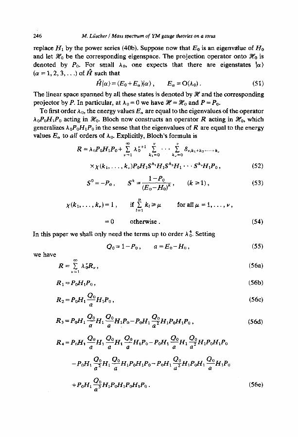
Let/-~r =Ho+AoHt be the hamiltonian in the Coulomb gauge (eqs. (40)), but consider A0 as an independent coupling constant. Bloch's method yields an expansion in powers of Ao. In the final expressions one may then set Ao = g2o/3 and

246 M. Liischer / Mass spectrum of Y M gauge theories on a toms

replace/-/1 by the power series (40b). Suppose now that Eo is an eigenvalue of Ho and let ~o be the corresponding eigenspace. The projection operator onto ~o is denoted by Po. For small Ao, one expects that there are eigenstates la) (or = 1, 2, 3 . . . . ) of H such that

nl~> = (E0 +tL)l~>, tL = O(ao). (51)

The linear space spanned by all these states is denoted by X a and the corresponding projector by P. In particular, at ho = 0 we have ~ = ~o and P = Po.

To first order ho, the energy values E~ are equal to the eigenvalues of the operator hoPoH~Po acting in ~o. Bloch now constructs an operator R acting in ~o, which generalizes h oPoH~Po in the sense that the eigenvalues of R are equal to the energy values E,, to all orders of Xo. Explicitly, Bloch's formula is

v = l k ,=O kv=O

× x (k l . . . . . kv)PoH1SklH1Sk2H1 • • • SkvH1Po, (52)

sO=_po, Sk= 1-Po (Eo-Ho) k ' (k t> 1), (53)

v~

x(k~ . . . . . k ~ ) = l , if ~ kt>~t~ /=1

for all tz = 1 . . . . . v,

= 0 otherwise. (54)

In this paper we shall only need the terms up to order A 04. Setting

we have Qo = 1 - P o , a = E o - H o , (55)

R = ~ A~R~, (56a)

R 1 = PoH1Po, (56b)

R 2 = Poll1 Q°H1Po, (56c) a

R3= PoH1Q° H 1 Q ° H1Po-PoH1 -Q-~-H1PoH1Po , a a a (56d)

R4= eonl O° n l O° O° H eo- eonl O° H eonlPo a a a a a

- P o n l - ~ H 1 Q ° H1P°H1P°- Q--~°2 Q°H1P°a

+ Poll1 Q-~H1PoH1PoH1Po. (56e) a

M. Liischer / Mass spectrum of Y M gauge theories on a torus 2 4 7

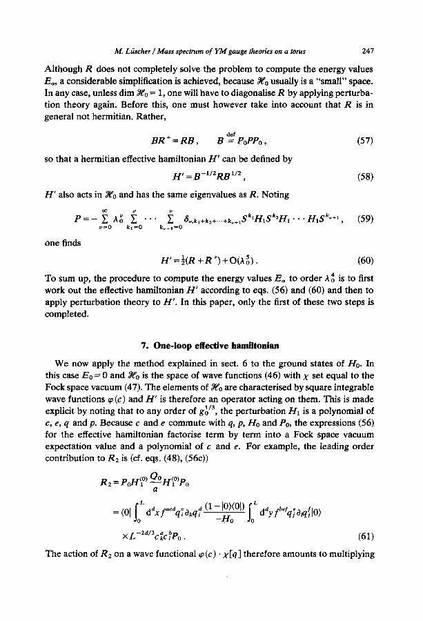
Although R does not completely solve the problem to compute the energy values E~, a considerable simplification is achieved, because ~'o usually is a "small" space. In any case, unless dim ~0 = 1, one will have to diagonalise R by applying perturbation theory again. Before this, one must however take into account that R is in general not hermitian. Rather,

dcf B R + = R B , B = PoPPo, (57)

so that a hermitian effective hamiltonian H ' can be defined by

H ' = B - 1 / 2 R B 1/2, (58)

H ' also acts in ~'0 and has the same eigenvalues as R. Noting

_ _ _ ~ Ao ~ " " ~ k, =-- v 8~.k~+k2+...+k~÷~S H i S H i " "H1S k ~ , (59) P v~O k l~O kv+l=O

one finds

H ' = ½(R + R +) + O(A 5o). (60)

To sum up, the procedure to compute the energy values E~ to order A 04 is to first work out the effective hamiltonian H ' according to eqs. (56) and (60) and then to apply perturbation theory to H ' . In this paper, only the first of these two steps is completed.

7. One-loop effective hamiltonian

We now apply the method explained in sect. 6 to the ground states of Ho. In this case Eo = 0 and ~t'o is the space of wave functions (46) with X set equal to the Fock space vacuum (47). The elements of ~o are characterised by square integrable wave functions ~o (c) and H ' is therefore an operator acting on them. This is made explicit by noting that to any order of g~/3, the perturbation H1 is a polynomial of c, e, q and p. Because c and e commute with q, p, Ho and Po, the expressions (56) for the effective hamiltonian factorise term by term into a Fock space vacuum expectation value and a polynomial of c and e. For example, the leading order contribution to R2 is (cf. eqs. (48), (56c))

R2 = PoI-t O° a

:(01 fo L daxffCaq~Okqdi (1--10)(01) I o ' - H o dayfbe:qTOtq~JO)

× L-2a/3c ~,c ~Po. (61)

The action of R2 on a wave functional ~o(c) • )~[q] therefore amounts to multiplying


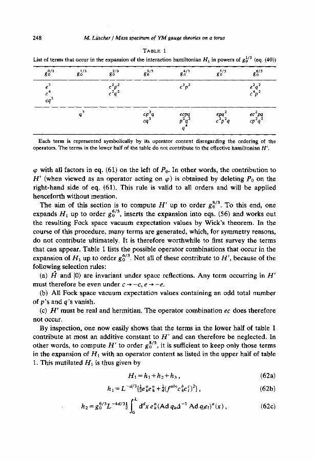
TABLE 1

List of terms that occur in the expansion of the interaction hamiltonian H1 in powers of g~/a (eq. (40))

gOo/a g10/3 g20/3 g~/3 g~/3 g~/3 g6o/3

e: c2p 2 cap 2 e2q 2 4 2 2 c4p2 c c q

cq 2

q 3 cp 2q ecpq epq 2 ec 2pq cq3 pZq2 c2p2q cp2q2

4 q

Each term is represented symbolically by its operator content disregarding the ordering of the operators. The terms in the lower half of the table do not contribute to the effective hamiltonian H'.

q~ with all factors in eq. (61) on the left of P0. In other words, the contribution to H ' (when viewed as an operator acting on ¢) is obtained by deleting P0 on the right-hand side of eq. (61). This rule is valid to all orders and will be applied henceforth without mention.

The aim of this section is to compute H ' up to order g0 s/3. To this end, one expands H1 up to order g6/a, inserts the expansion into eqs. (56) and works out the resulting Fock space vacuum expectation values by Wick's theorem. In the course of this procedure, many terms are generated, which, for symmetry reasons, do not contribute ultimately. It is therefore worthwhile to first survey the terms that can appear. Table 1 lists the possible operator combinations that occur in the expansion of H1 up to order g~/3. Not all of these contribute to H ' , because of the following selection rules:

(a) /~r and 10) are invariant under space reflections. Any term occurring in H ' must therefore be even under c ~ - c , e -~ - e .

(b) All Fock space vacuum expectation values containing an odd total number of p's and q's vanish.

(c) H ' must be real and hermitian. The operator combination ec does therefore not occur.

By inspection, one now easily shows that the terms in the lower half of table 1 contribute at most an additive constant to H ' and can therefore be neglected. In other words, to compute H ' to order gS/3, it is sufficient to keep only those terms in the expansion of H1 with an operator content as listed in the upper half of table 1. This mutilated H1 is thus given by

H1 = hi + hE + h 3 , (62a)

T--d/3rl a a- - l J , , . abe b c,.2"~ h l = L t gekek~-Z t l C ~ ) I , (62b)

L o h2 -- go6/3r-4a/311-, 2 | dax e ~ (Ad qk A-1 Ad qlet) ~ (x) , (62c)

Jo

M. Liischer / Mass spectrum of Y M gauge theories on a torus

L

H o + g2/Sh3 = ½ Io dax {pkAktPt + qkBklql} ,

-- 8 + -4/3L-2d/3 1 " 1 A k l -- kl SO Ad Ck - ~ d Ad ct,

249

(62d)

(63a)

Bkt = -SktD'~Di +g4/3L-2a/a(Ad Ck Ad c1-2[Ad Ck, Ad ct]). (63b)

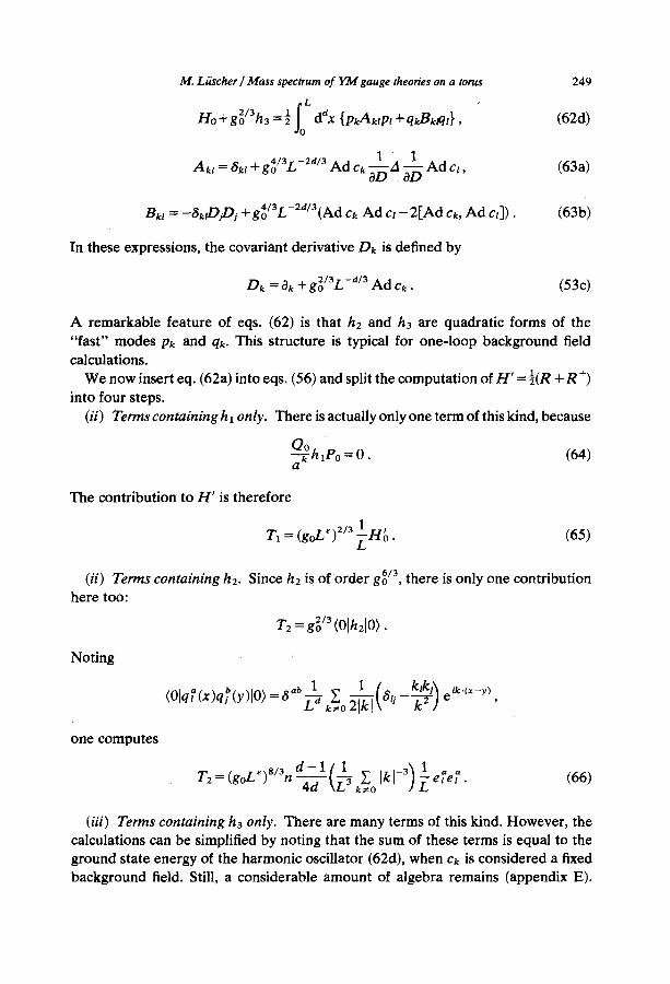
In these expressions, the covariant derivative D k is defined by

D k = t~k "4- g2o/3L-a/3 Ad Ck . (53c)

A remarkable feature of eqs. (62) is that h2 and ha are quadratic forms of the "fast" modes Pk and qk. This structure is typical for one-loop background field calculations.

We now insert eq. (62a) into eqs. (56) and split the computation of H ' = ½(R +R +) into four steps.

(ii) Terms containing h i only. There is actually only one term of this kind, because

-Q-~h 1P0 = 0. (64) a

The contribution to H ' is therefore

2/3 1 , T1 = (goL) ~ H 0 . (65)

(ii) Terms containing h2. Since h2 is of order g6/a, there is only one contribution here too:

Noting

Tz= g2o/3 (Olh210> .

1 8 klk!~ (OIq~(x)q~(y)lO)=Sab--~a k~O2-~l( t , e ~k''x-') -T:]

one computes

T2=(g°L~)S/3n 4d \ L k~,O ]kl-3 1 -~ e l e l . (66)

(iii) Terms containing h3 only. There are many terms of this kind. However, the calculations can be simplified by noting that the sum of these terms is equal to the ground state energy of the harmonic oscillator (62d), when ck is considered a fixed background field. Still, a considerable amount of algebra remains (appendix E).

250 M . Li i scher / M a s s spectrum o f Y M gauge theories on a torus

The outcome is

,,4/3 ( d - 1)2/1 1 V3= (goL ) ) a l l -~ClCl

)1 +(g°L~)S/3n 96d \L 3 kE~o Ikl-3 (f:%Pc;)2

d - ~ l 1 d)a,,,~,m Lk 14- 5dk~ksk~k,,,]) + (goL~) s/3 1-'-~- [,~--~ k~,O Ik I-7[(6-

1 abcd a b c d x-£s ClCsCiCr,. (67)

(iv) Terms containing hi and h3. Because of eq. (64) such a combination can only occur in R3 and R4. It turns out that the rules (a) and (c) above exclude a contribution from R3 and one is left with

7"4--~s/3![/0 t ' s o 2/, i t i3 -~[h l , [h l , h3]]10)+(0i[hl,[hx, h3]]-~ha,0)}

Noting L

h3=L-al3c~ Io d% f"%f:(x)a~(x)+ 213 O(g0 ),

one obtains (after some algebra)

d - l ( 1 ikl_3) l ,be b ~2 T4=-(goL~)S/3n-i-~\-~k~o -~(f c~ci) . (68)

Finally, the contributions T~, i = 1 . . . . . 4, are added up and the following result is obtained:

k@O / . I "~ - ' £e l e l

+ (g°Le)2/3 [ 1 + (g°L~)2n -d2+24dd+ 24 ( ~ k ~ O Ikl-3)] l(fabccblc~)2

( d - 1 ) ~ ( 1 ~ ikl_,) 1 o . + (goL~)4i3n ~ k - ~ kL ° ~c,c,

d - l / 1 ikl_7[(6_d)8,,.&.lkl,~_ 5dk,ksk,k,,,]) +

1 abcd a b c d x-~s CtCsCiC,.,. (69)


eae a / , . a b e b cx2 As is seen f rom this formula, the coefficients of t t and t f c~c~) are not the same. This asymmetry can be removed by rescaling Ck, i.e. by making the substi- tution*

c~ -, Z1/~ c~ a ~ . - 1 / 2 , e k ~/-~ ek , (70a)

d 2 + t l d - 3 6 / 1 [k[_3) Z= l _ + ' " (70b)

After that H ' assumes the simple form

H ' = (g°Z~)E/3{Hto +(go/-- ~'2/31 al~k~k~-~ L

a b c d a b c d - a b c d a b ¢ d ' l~ +(goL~)6/a[ot2H~ +a3s C k C k C l C l "l-Ol4S CkCkCkCkJ~, (71)

( d - l ) 2 1 ~ [kl_ 1 (72a) a l = n 4-----d-- L k,,O '

2 5 - d 1 0g 2 ~--- n 7---~ L 3 ~ lkl-3 ' (72b)

k ~ 0

d - 1 1 a3 = 16---d- L 3 ~" Ik[-7[(6-d)[k[4- 15dk 2k 2]' (72c)

k ~ 0

5 ( d - 1) 1 a 4 = 16 L 3 y [kJ-7(k4-ak21k2)" (72d)

k # 0

To go f rom here to the effective hamiltonian as quoted in sect. 1, it remains to evaluate the one- loop m o m e n t u m sums in the coefficients al. Following the rules of dimensional regularisation**, the sums are first rewritten with the help of the heat kernel on $1:

f ( t ) = exp {-t(2rr•)2}, (73)

L---; k~,o ~ Ik[- '= ~ d t t ~ - l ( f a - 1) . (74)

The coefficients ai then become

( d - 1) 5 f ~ ax = n ~ jo d t t - 1 / 2 ( f a - 1 ) ' (75a)

25-d f ~ t l /2 ( f a _ a E = n ~ j 0 dt 1), (75b)

* Only the spectrum of H' is observable; this is not affected by a change of variables. ** For more details about dimensional regularisation with compact dimensions see e.g. ref. [10].

252 M. Liischer / Mass spectrum of YM gauge theories on a torus

d - 1 fo~ c~3 = 30-'6-~ ,I ° d t t S / 2 [ ( 6 - d ) f a - l f " - ( d 2 - 7 d + 2 1 ) f a - 2 ( l c ' ) 2 ] , (75c)

d - l I : o~4 =, ~ df ts/2[fa-lf "- 3fa-2(f')2]. (75d)

Some properties of the heat kernel on S I are listed in appendix B (in the notation

used there [(t) = F,(O; I)). It follows from these that the coefficients o~i are meromor- phic functions of d, the representations (75) being valid for low Re d. Only o~2 has

a pole at d = 3:

l l n 1 a 2 = 9(4~r) 2 e I-O(1). (76)

This pole is exactly cancelled by the coupling constant renormalization (11). In other words, H ' as given by eq. (71) is finite at d = 3, provided only the coupling constant is renormalized in the usual way. It is not difficult to compute the finite part of t~2 and the values of the other ~t's at d = 3 (see appendix F for a sample calculation). With this last step completed, the effective hamiltonian as presented in sect. 1 is obtained.

We conclude this section by remarking that the effective hamiltonian for the 2 + 1 dimensional theory can be quickly obtained from the above formulae simply by evaluating the a ' s at d = 2 (there are no poles there and the coupling constant need not be renormalized). At d = 1 the expected null result is obtained.

8. Concluding remarks

The calculations in this paper rely on the Schr~dinger representation, i.e. on the use of wave functionals and of the Hamilton operator. The Schr/Sdinger representation of the t~ 4 theory was recently investigated by Symanzik [1 I]. He found that, as expected, all amplitudes were well defined in the dimensionally regularised theory and that, furthermore, the wave functionals could be renormalized so as to make them finite and non-trivial in the cutoff free theory. To the extent that no unexpected ultraviolet divergencies were encountered, the results obtained here show that the same is true in the gauge theory case, too. It is possible to compute the effective hamiltonian /-/" by a purely euclidean method. Namely, one first calculates the euclidean transition amplitude to go from a constant gauge field to another in perturbation theory and expands for large times T. H ' can then be read off essentially from the term proportional to T. Using the Lorentz gauge, I computed the one-loop coefficients o~i along these lines and reproduced eqs. (75). One may therefore be confident that the hamiltonian method not only yields finite but also correct results. From the calculational point of view, the euclidean and the hamiltonian technique are about equally voluminous. However, most of the steps necessary to compute the effective hamiltonian are programmable (the expansion

M. Lfischer / Mass spectrum of YM gauge theories on a torus 253

of H and Bloch's formulae, for example) so that one may very well be able to go beyond the one-loop level.

A striking result of the present investigation is the exact degeneracy of the central sectors to all orders of perturbation theory. This is a truly non-linear effect, which does not take place in the abelian gauge theory, where the sectors are split by

energy gaps proportional to g2/L . From lattice gauge theories (or the "electric flux" interpretation [5]) one expects, on the other hand, that the gaps in the non-abelian case increase with L. While such a behaviour would be difficult to obtain in perturbation theory, a non-perturbative contribution always is accom- panied by a power L p, where p can be any number greater than - 1 . For this reason, the perturbative degeneracy of the central sectors is welcome and one may even hope to estimate the string tension by computing the non-perturbative splitting of the sectors semi-classically.

Many of the technical difficulties that arise when perturbation theory is applied to gauge fields on a torus are due to the existence of torons. I therefore first considered to calculate the energy spectrum for gauge fields confined to a sphere S 3, which is simply connected and does not allow for toron solutions. However, this possibility must be dismissed for another reason: S 3 is a curved space so that relative to the infinite volume theory the wave functions are distorted locally. T h e

approach of the finite volume masses to the infinite volume values is therefore slow (i.e. like 1 / L instead of exp ( - m L ) ) and there would be little hope to extract accurate numbers for the mass ratios from perturbation theory (see ref. [1] for further discussion).

Practically all results obtained in this paper carry over to gauge theories on a finite periodic lattice. In particular, central sectors, torons and the effective hamiltonian H ' exist as before. To lowest order, H ' is still equal to H~, but the one-loop coefficients a,. now depend on L in a way, which is specific to the particular lattice action chosen.

A p p e n d i x A

SU(n) NOTATIONS

The Lie algebra au(n) of SU(n) consists of all complex n × n matrices X with

X + = - X , T r X = 0 . (A.1)

Let T a, a = 1 . . . . . n 2 - 1 , be a basis of such matrices satisfying

Tr ( T a T b) = -½8 ab . (A.2)

The structure constants fabc and the totally symmetric tensor d *be are then defined

by

I T ~, T b ] =f°bCTC, (A.3)


{T" , T b} = - 1 8 " b + id~b~T ¢ . n

Both tensors are real and

(A.4)

we have

dadedbde = __1 (n 2 -7 4 )8 ~b. ( A . 6 )

The totally symmetric tensor s ~b~d, which occurs in the effective hamiltonian (eq. (3e)), is given by

s ~bcd = ~ n (d~bed ~d~ + d ~ d bde + d~ded bc~)

"F 2(8 ab8 cd "F" 8 ac8 bd dr" 8 ads be ) . (A.7)

Its group theoretical meaning is explained below. For any X ~ oa(n) define a linear mapping

A d X : ou(n ) --> o , ( n ) , (A.8)

A d X ( Y ) = [X, Y] for all Y ~ o , ( n ) .

With respect to the basis T ~, Ad X is represented by a matrix (Ad X ) ~ so that

A d X ( T b) = T~(Ad X ) ~b . (A.9)

Explicitly, writing

X = X ~ T ~ , (A. 10)

(Ad X ) ~b = f~cbXC, (A. 11)

(Ad X(Y))~ = (Ad X ) ab y b . (A. 12)

The matrices (Ad X ) ~b form the adjoint representation of og(n). In particular,

lAd X, Ad Y] = Ad IX, Y], (A.13)

Tr (Ad X Ad Y) = 2n Tr ( X Y ) . (A.14)

The meaning of the symbol s ~bcd is now made clear by the following L e m m a : Let X1 . . . . . X4 be four elements of o¢(n). Then

1 - - abcd-ffira ~rb ~.c .~1d ~ T r ( A d X ~ ( 1 ) A d X ~ ( 2 ) A d X ~ ( 3 ) A d X ~ ( 4 ) ) = s A I A 2 A 3 A 4 , (A.15)

4~

where tr runs over all permutations of (1, 2, 3, 4). Proof: For any choice of real numbers Ai set

4 X-~-- E A i X i .

i=1

f~defbd~ = n8 =b , (A.5)

M. Liischer / Mass spectrum o f Y M gauge theories on a torus

The left- and right-hand sides of eq. (A.15) can then be written as

1 O 4 lhs = - - T r (Ad X) 4 ,

4! c~A1 c3A20A30A4

1 0 4 = - - . $ a b c d x a x b x c x d .

rhs 4! tgA1 0A2 0A3 0A4

It is therefore sufficient to show that

Tr (Ad X ) 4 = s~b~dx°xbx~x d ,

for all X ~ o~(n). To this end, first note that

Tr (exp Ad X) = - 2 Tr ( T ~ eXT ~ e - x )

= (Tr eX)(Tr e -x ) - 1.

Identifying the terms of order X 4 we have

Tr (Ad X) 4 = 2n Tr X 4 + 6(Tr X2) 2 .

Finally, using eq. (A.2) and

X 2 1 x a x a _ 1. Jab . . . . . b,-~c = - - -l- ~ ta A A 1 , 2n

one obtains

as required. []

Tr (Ad X) 4 = ¼ndaOedcdexaxbxcx a + 2 ( s a g a ) 2

= s abcnX"XbXCX d '

Appendix B

HEAT KERNEL ON S 1

The heat kernel on S 1 is defined by (t > 0, z ~ C)

1 ~ f /2,rv'x 2 .2zrv ) F , ( z ; L ) = - ~ ~ oexp l , t ( - -~ - - ) +t--'~--z~ .

It is the fundamental solution of the heat equation on $I:

F,(z + L ; L) = Ft(z ; L ) ,

l i m F t ( z ; L ) = ~ 8 ( z - v L ) , ( z e R ) ,

255

(B.1)

(B.2)

(B.3)

(B.4)

256 M. Liischer / Mass spectrum of YM gauge theories on a toms

Using the Poisson s u m m a t i o n fo rmula one obta ins

1 Fr(z ;L) - - (4~r t ) - l /2 ~ooexp { - ~ - ~ ( z - v L ) 2 } •

For real z, Ft(z ; L ) is hence real and posit ive. F u r t h e r m o r e 2

F t ( O ; L ) = ( 4 ~ ' t ) - l / 2 { l + O ( e x p [ - L ] ) } ,

2 F t ( O ; L ) - - - ; 1 , ( t . o o ) .

(B.5)

(t-~ 0 ) , (B.6)

(B.7)

Appendix C

COMPUTATION OF fgo[¢]

W e first de t e rmine the e igenvalues of / '2 [¢ ]. This is easy, because the to ron field Ak[~o] is i ndependen t of x. T h e e igenfunct ions o f / 2 [ ¢ ] are the re fo re p lane waves:

q~(x) = V'; e ik'~ , (C.1)

2~r kj = -~-- vj, u j e Z , (C.2)

T h e e igenvalue equa t ion and the gauge condi t ion (23b) then b e c o m e algebraic:

(kl - i A d At[~p ])2vi = Ev j , (C.3)

(kl - i A d A~[¢])vr = 0 . (C.4)

T h e condi t ions (23a) requires tha t the th ree matr ices vl have zeros on their d iagonal

if k = 0. The matr ices A d At[q~] c o m m u t e and can be s imul taneous ly diagonalised. This solves eq. (C.3). T h e constra int (C.4) mere ly reduces the multiplicit ies of the ene rgy levels by 1". T h e result is:

Eo(k) = k 2, k ~ 0 , mult ipl ici ty 2(n - 1 ) , (C.5)

1 ,, a \2 E ~ a ( k ) = k t+-~(¢ t - ¢ z )) , a # f l , mul t ip l i c i t y2 . (C.6)

W e now compu te g0[t0] using Paul i -Vi l lars regulators . The reason for not using d imens ional regular isat ion is the la tent danger inheren t to this m e t h o d tha t ~o- d e p e n d e n t terms, which are m o r e than logar i thmical ly divergent , are regular ized to zero. Thus, let Mj and ej (j = 1 . . . . . v) be regula tor masses and a l te rnat ing signs such that

i ej = - 1 , i e//~/~ p = 0 , (p = 1, 2 . . . . . V -- 1) . (C.7) j= l /=1

* Strictly speaking this is only true if E > O. However, zero modes occur only for torons Ak[¢] at the boundary of the toron manifold and even in that case it is not necessary to count them correctly, because they do not contribute to gPo[¢]-

M. Liischer / Mass spectrum of Y M gauge theories on a torus 2 5 7

Then the regularized frequency sum is

$o[¢]= Y Z{fffaa(k)+ ~ eiJEaa(k)+M~}. (C.8) a # ~ k 1=1

Here and below all terms not depending on ¢~' are dropped. Noting

we have

dt t -3/2 ei e ,) e -ns , (C.9) / = 1 '=

{ , . }) ~ e - 'E-#k)= f i ( ~ exp ---~(21rv,+~ot-~0~) 2 , / = 1 vl ~--co

(c.lo)

$o[¢]= ~BF(_½)I?dtt-3/2(l+ ~ le~e-~ )

{ ' o }) x 1"[ exp -~--~(2~'vl +~ l -~o~) 2 . (CAD / = 1 vl co

Next, the sums are converted using Poisson's summation formula (cp. appendix B):

v! ~ -co

L ~ exp{--~(vlL) +iVl(¢t--gOal)} (C.12)

When inserted into eq. (C.11) one then sees that only the term with vl = v2 = v3 = 0 is ultra-violet divergent. But this term is also independent of ¢~ so that the interesting e-dependent part of g'o[C¢ ] is convergent for Mj -> oo. Furthermore, the t-integral becomes elementary in this limit and the final result is

1 $ ' o [ ¢ ] = - - - - ~ X Z (v2) - 2 c o s y " ( C a _ C a ) , (C.13)

7/" /--, a # B v # O

(the minus sign stems f rom/"(-½) = - 4x/~; v denotes the integer vector (vl, v2, v3) and q~ = (~p ~', ~ ,2, ¢3)).

Appendix D

S P E C T R U M O F H ~

The proof of the theorem in sect. 5 is based on a criterion valid for general Schr6dinger operators

A = --A + V, (D.1)


where V >~ 0 is a continuous function on R". Under these conditions, A is essentially self-adjoint on C~(R "~), the space of all infinitely differentiable wave functions S (x) with compact support (ref. [8], theorem 10.28). This means that A extends from C~(R m) to a unique self-adjoint operator, which will also be denoted by A.

Criterion: Suppose there is a continuous function A (x)(x ~ R r~) such that A/>0 and

(S, AS) ~> I d"x a (x) lS(x) l z , for all S ~ C~ ( R" ) . (D.2)

Suppose furthermore that A (x) -~ oo as x ~ ~ . Then, A has purely discrete spectrum. This criterion follows easily from a formula for the bottom of the essential

spectrum of A quoted by Agmon [9]. Alternatively, one may adapt the proof of theorem 13.16 of ref. [8], which treats the case where the potential V itself goes to infinity in all directions (i.e. in this case one may choose A = V).

It remains to find a function A for H~. To this end, note that the potential V (eq. 50) can be written as

d V ( C ) = a t n a b b ,,,,,abc b cx2 c 1 ~ c1+½ ~. (D.3) ~ f CkC]) ,

k j=2

d M ~b= E (f"*ec~)(fbd~C~),

k=2

It follows that for any 0 ~ C~

02 c~M"bc~) S(c)

(D.4)

one thus obtains

Now, M is symmetric with eigenvalues to 2 t> 0 (a = 1 . . . . . n 2-1) . Furthermore, M is independent of cl so that at fixed Ck, k >/2, the operator on the right-hand side of eq. (D.5) is just a harmonic oscillator hamiltonian with frequencies toa. Performing the cl integrations first, it follows that*

Noting

Xtoa~ > to,} = ( T r M ) l /z= n ~ CkCk} , (D.7) a k=2

/ a \ 1 / 2

(S,H'oS)>~½v~n [ dc[k~,2c~,c~, ) IS(c)[ 2 . (D.8)

* This is the crucial step in the proof. It realizes the intuitive insight that wave functions in narrow potential valleys have high energy, because the kinetic term forces them to spread into regions where the potential is not small.

(D.6)

(D.5)


Finally, the estimations are repeated with cl replaced by c2 etc. and the resulting inequalities (D.8) are then averaged. This yields the symmetric bound

(4,,H~J/)>~l ~ f dc(c~c~)1/214/(c)12. (D.9)

Hence

x (c) = 1 J n ( d - 1)(c ~c ~)1/2, (D. 10)

has all the properties necessary for the criterion to apply.

A p p e n d i x E

COMPUTATION OF T3

The ground state energy of the harmonic oscillator (62d) is given by

T3 = ½ Tr' {[(PAP)a/uB(PAP)I/2]I/2}. (E.1)

Here, P denotes the proiector

Pkl = ~kl --Ok A- l Ol , (E.2)

and Tr' {. • .} means the trace over the space of periodic functions f~(x) with

L

Io ddx f~ (x ) = O. (E.3)

In a condensed notation, we have from eqs. (63)

1 (PAP) 1/2 = P + ½(goL')'/3 ~ p . A d c ~-~-A ~ A d c . P

-~(goL~) 8/3 P.Adc-~--~A-~--~Adc. + . . . , (E.4)

= P ( - A ) P - (goLe) 2/3 2 p Ad c " OP PBP

- (goL ~)4/3 ~22 (P A d c • Ad cP - P " A d c A d c • P + 2 P ' lAd c, Ad c ]" P ) .

Furthermore, using

1AOD ~OD ---- A-1 -- (g°Le)2/3 2 A -1 Ad c . 0A -1

+ (goL~)4/3 3 A - 1 A d c • aA-1Adc • aA-l+ . . ' , (E.6) L

260 M. Liischer / Mass spectrum o f Y M gauge theories on a torus

one first obtains (PAP)I /2B(PAP) 1/2 and then the square root of this operator as a power series of g2o/3. A typical term in the latter expansion is

X = ( - A ) - 3 / 2 P A d c ' 0 A d c • 0P. (E.7)

The trace of such operators is easily worked out in momentum space:

T r ' X = - ( d - 1) Y. {kl-3klkj Tr (Ad c~ Ad cj) k~0

d - 1 E Ikl - ' Tr (Adct A d c , ) . (E.8)

d k#0

Here, the trace on the right-hand side refers to color only. Up to an additive constant, the outcome then is

1"3 = -(goL~) 4/3 12 ( d - 1) 2 ~ Ikl_~ Tr (Ad c~ Ad ct) 4d k~0

_ ( g o L , ) S / 3 1 ~ 1 ~ [kl_ 3 Tr ([Ad ct, Ad cj3[Ad c,, Ad cj]) L [4d k~O

* ( d - 1 ) ( d - 6 ) ~ ikl_ 3 Tr (Ad ct Ad ct Ad cj Ad cj) 16d k~o

+ 5 ( d - l ) ~ [kl_Tktkjkikm T r ( A d c t A d c j A d c i A d c m ) } . (E.9) 16 k~0

Finally, using some identities from appendix A, one finds

Tr (Ad ct Ad cl) = -nc':c '~, (E.10)

Tr (Ad ct Ad cl Ad ci Ad cj)

a b c d a b c d 1 = s c~clc j cj - g t r (lAd ct, Ad cj][Ad ct, Ad cj]),

Tr ([Ad ct, Ad cj][Ad cl, Ad ci]) = , ~abc b c,2 - -nl , f C t C j ) ,

T r ( k A d c ) 4 . . . . . bed ~ b c d • =KII~jKiKm S C l C j C i C m •

(E.11)

(E.12)

(E.13)

When these relations are inserted into eq. (E.9), one obtains the result quoted in sect. 7.

Appendix F

E V A L U A T I O N OF a l AT d = 3

Define

v ~ - - o o

(FA)

M. Lg~scher / Mass spectrum of YM gauge theories on a torus

The coefficient al is then given by (cf. eq. (75))

( d - 1) 2 o t l = n ~ j ° dtt-a/2(ha-1), R e d < l .

Using the duality relation (B.5),

we have

261

(F.2)

(F.3)

Io ld t t - (h - 1 ) = - 2 + j 1 ~°dt f 1 /2 d t~a-3)/2 h d

2 d ~oo dt t(d-3)/2(h d = - d _ l + J l - 1 ) .

I t fo l lows tha t

( d - 1)2f 2 d ~ t(a-3)/Z)(h a 1)} . ax = n ~ - ~ - L - - ~ + f l a t ( t - I / 2 + (F.4)

This representation is valid for all d. In particular,

Finally, substituting the series (F.1) for h and performing the integral numerically, one gets

~lla=3 = - ~ - 1.89153165 . . . . (F.6)

References

[1] M. Lfischer, Phys. Lett. 118B (1982) 391 [2] G. 't Hooft and M. Veltman, Nucl. Phys. B44 (1972) 189;

G. 't HoG(t, NucL Phys. B61 (1973) 455 [3] C. Bloch, Nucl. Phys. 6 (1958) 329 [4] J.D. Bjorken, Elements of quantum chromodynamics, in Proc. Summer institute on particle physics,

ed. Anne Mosher, SLAC report no 224 (1980) [5] O. 't HoG(t, Nucl. Phys. B153 (1979) 141 [6] A. Oonzalez-Arroyo, J. Jurkiewicz and C.P. Konhals-Altes, Ground state metamorphosis for

Yang-Mills fields on a finite periodic lattice, Marseille preprint (1981), in Proc. of the Freiburg NATO Summer Institute (Plenum, 1981) to appear

[7] N.M. Christ and T.D. Lee, Phys. Rev. D22 (1980) 939 [8] M. Reed and B. Simon, Methods of modern mathematical physics, vols. 1--4 (Academic Press,

New York 1972) [9] S. Agraon, How do eigenfunctions decay? The case of N-body quantum systems, lecture notes in

physics 153, p. 142 (Springer, 1982) [10] M. Liischer, Ann. of Phys. 142 (1982) 359 [11] K. Symanzik, Nucl. Phys. B190 [FS3] (1981) 1

SOME ANALYTIC RESULTS CONCERNING THE MASS SPECTRUMjpac/QCDRef/1980s/SOME ANALYTIC... · SOME...

Documents

Transcript of SOME ANALYTIC RESULTS CONCERNING THE MASS SPECTRUMjpac/QCDRef/1980s/SOME ANALYTIC... · SOME...