Some additional Topics

Distributions of functions of Random Variables

Gamma distribution, 2 distribution, Exponential distribution

TheroremLet X and Y denote a independent random variables each having a gamma distribution with parameters (,1) and (,2). Then W = X + Y has a gamma distribution with parameters (, 1 + 2).

Proof:

1 2

and X Ym t m tt t

1 2 1 2

t t t

Therefore X Y X Ym t m t m t

Recognizing that this is the moment generating function of the gamma distribution with parameters (, 1 + 2) we conclude that W = X + Y has a gamma distribution with parameters (, 1 + 2).

Therorem (extension to n RV’s)

Let x1, x2, … , xn denote n independent random variables each having a gamma distribution with parameters (,i), i = 1, 2, …, n. Then W = x1 + x2 + … + xn has a gamma distribution with parameters (, 1 + 2 +… + n). Proof:

1, 2...,i

ixm t i nt

1 2 1 2 ...

...n n

t t t t

1 2 1 2... ...

n nx x x x x xm t m t m t m t

Recognizing that this is the moment generating function of the gamma distribution with parameters (, 1 + 2 +…+ n) we conclude that

W = x1 + x2 + … + xn has a gamma distribution with parameters (, 1 + 2 +…+ n).

Therefore

TheroremSuppose that x is a random variable having a gamma distribution with parameters (,). Then W = ax has a gamma distribution with parameters (/a, ). Proof:

xm tt

then ax xam t m at

at ta

1. Let X and Y be independent random variables having an exponential distribution with parameter then X + Y has a gamma distribution with = 2 and

Special Cases

2. Let x1, x2,…, xn, be independent random variables having a exponential distribution with parameter

then S = x1+ x2 +…+ xn has a gamma distribution with = n and

3. Let x1, x2,…, xn, be independent random variables having a exponential distribution with parameter

then

has a gamma distribution with = n and n

1 nx xSx

n n

0

0.1

0.2

0.3

0.4

0.5

0.6

0 5 10 15 20

pop'n

n = 4

n = 10

n = 15

n = 20

Distribution of population – Exponential distribution

x

Another illustration of the central limit theorem

4. Let X and Y be independent random variables having a 2 distribution with 1 and 2 degrees of freedom respectively then X + Y has a 2

distribution with degrees of freedom 1 + 2.

Special Cases -continued

5. Let x1, x2,…, xn, be independent random variables having a 2 distribution with 1 , 2 ,…, n degrees of freedom respectively then x1+ x2 +…+ xn has a 2 distribution with degrees of freedom 1 +…+ n.

Both of these properties follow from the fact that a 2 random variable with degrees of freedom is a random variable with = ½ and = /2.

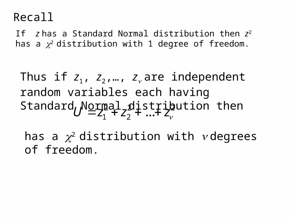
If z has a Standard Normal distribution then z2 has a 2 distribution with 1 degree of freedom.

Recall

Thus if z1, z2,…, z are independent random variables each having Standard Normal distribution then

has a 2 distribution with degrees of freedom.

2 2 21 2 ...U z z z

TheroremSuppose that U1 and U2 are independent random variables and that U = U1 + U2 Suppose that U1 and U have a 2 distribution with degrees of freedom 1and respectively. (1 < )Then U2 has a 2 distribution with degrees of freedom 2 = -1 Proof:

12

1

12

12

Now

v

Um tt

21

2

12

and

v

Um tt

1 2

Also U U Um t m t m t

2

12 2

12

12

1122

11 22

12

v

vv

v

tt

t

2

1

Hence UU

U

m tm t

m t

Q.E.D.

Bivariate DistributionsDiscrete Random Variables

The joint probability function;

p(x,y) = P[X = x, Y = y]

1. 0 , 1p x y

2. , 1x y

p x y

3. , ,P X Y A p x y ,x y A

Marginal distributions

,Xy

p x P X x p x y

,Yx

p y P Y y p x y

,

X YY

p x yp x y P X x Y y

p y

,

Y XX

p x yp y x P Y y X x

p x

Conditional distributions

The product rule for discrete distributions

,Y X Y

X Y X

p y p x yp x y

p x p y x

Independence

, X Yp x y p x p y

Bayes rule for discrete distributions

X Y X

X YX Y X

u

p x p y xp x y

p u p y u

Proof:

,

X YY

p x yp x y

p y

,

,u

p x y

p x u

X Y X

X Y Xu

p x p y x

p u p y u

Continuous Random Variables

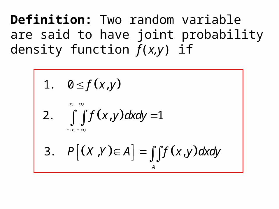
Definition: Two random variable are said to have joint probability density function f(x,y) if

1. 0 ,f x y

2. , 1f x y dxdy

3. , ,P X Y A f x y dxdy A

Marginal distributions

,Xf x f x y dy

,Yf y f x y dx

Conditional distributions

,

Y XX

f x yf y x

f x

,

X YY

f x yf x y

f y

The product rule for continuous distributions

,Y X Y

X Y X

f y f x yf x y

f x f y x

Independence

, X Yf x y f x f y

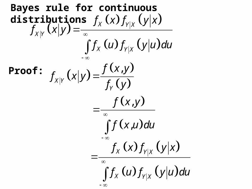
Bayes rule for continuous distributions

X Y X

X Y

X Y X

f x f y xf x y

f u f y u du

Proof:

,

X YY

f x yf x y

f y

,

,

f x y

f x u du

X Y X

X Y X

f x f y x

f u f y u du

Example• Suppose that to perform a task we first have to

recognize the task, then perform the task.

• Suppose that the time to recognize the task, X, has an exponential distribution with l = ¼ (i,e, mean = 1/ = 4 )

• Once the task is recognized the time to perform the task, Y, is uniform from X/2 to 2X.

1.Find the joint density of X and Y.

2.Find the conditional density of X given Y = y.

Now

, X Y Xf x y f x f y x

and

141

4

22

2

0

0 0

1 22

2 3

0 or 2

x

X

xx

Y Xx

e xf x

x

y xx xf y x

y x y

141 2

4 3 20, 2

0 otherwise

x xxe x y x

141

6 20, 2

0 otherwise

x xx e x y x

Thus

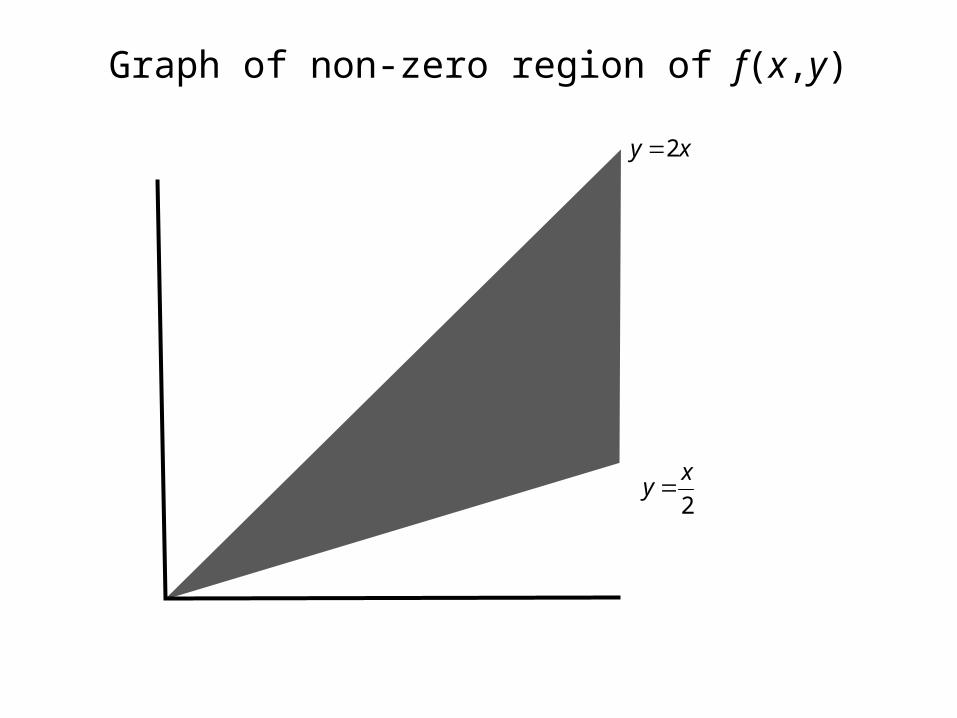
Graph of non-zero region of f(x,y)

2y x

2

xy

Bayes rule for continuous distributions

X Y X

X Y

X Y X

f x f y xf x y

f u f y u du

2y x

2

xy

2 ,y y

,2

yy

1 14 4

1 14 4

2 2

1 16

22 2

1 16

2 , 0

y y

x xyx x

y yu u

u u

e ex y y

e du e du

Conditional Expectation

Let U = g(X,Y) denote any function of X and Y.

Then

,E U x E g X Y x

, Y Xg x y f y x dy

h x

is called the conditional expectation of U = g(X,Y) given X = x.

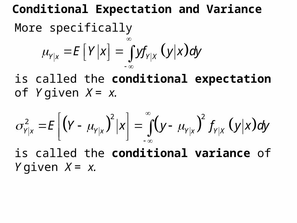
Conditional Expectation and Variance

More specifically

Y x Y XE Y x yf y x dy

is called the conditional expectation of Y given X = x.

2 2

2Y x Y x Y x Y XE Y x y f y x dy

is called the conditional variance of Y given X = x.

An Important Rule

, XE U E g X Y E E U x

where EX and VarX denote mean and variance with respect to the marginal distribution of X, fX(x).

X XVar U E Var U x Var E U x

and

Proof Let U = g(X,Y) denote any function of X and Y.

Then

,E U x E g X Y x , Y Xg x y f y x dy

h x

X X XE E U x E h X h x f x dx

, XY Xg x y f y x dy f x dx

, XY Xg x y f y x f x dxdy

, , ,g x y f x y dxdy E g X Y E U

Now

22Var U E U E U

22X XE E U x E E U x

22

X XE Var U x E U x E E U x

22

X X XE Var U x E E U x E E U x

X XE Var U x Var E U x

Example• Suppose that to perform a task we first have to

recognize the task, then perform the task.

• Suppose that the time to recognize the task, X, has an exponential distribution with = ¼ (i,e, mean = 1/ = 4 )

• Once the task is recognized the time to perform the task, Y, is uniform from X/2 to 2X.

1.Find E[XY].

2.Find Var[XY].

Solution

22 54

2

2

xxE XY x xE Y x x x

254X XE XY E E XY x E X

22 2

14

232

for the exponential distribution with

XE X

25 54 4Thus 32 40XE XY E X

222 2 2

12

xxVar XY x x Var Y x x

2324 4 45 45 15

4 6416 1212x x x

415 15464 64X XE Var XY x E X

4

15 15 2464 644 1

4

4!60 24

2 25 254 16X X XVar E XY x Var X Var X

2 22 4 2

2X X XVar X E X E X

4

2424 4

4 2 14

4! 2!20 4

and X XVar XY E Var XY x Var E XY x

60 24 8000 1440 8000 9440

42516hence 20(4 ) 8000XVar E XY x

Conditional Expectation:

k (>2) random variables

Let X1, X2, …, Xq, Xq+1 …, Xk denote k continuous random variables with joint probability density function

f(x1, x2, …, xq, xq+1 …, xk )

then the conditional joint probability function

of X1, X2, …, Xq given Xq+1 = xq+1 , …, Xk = xk is

Definition

11 11 1

1 1

, , , , , ,

, ,k

q q kq q kq k q k

f x xf x x x x

f x x

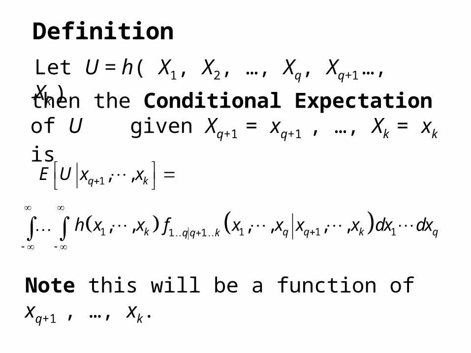
Let U = h( X1, X2, …, Xq, Xq+1 …, Xk )

then the Conditional Expectation of U given Xq+1 = xq+1 , …, Xk = xk is

Definition

1 1 1 11 1 , , , , , ,k q q k qq q kh x x f x x x x dx dx

1 , , q kE U x x

Note this will be a function of xq+1 , …, xk.

Example

Let X, Y, Z denote 3 jointly distributed random variable with joint density function

2127 0 1,0 1,0 1

, ,0 otherwise

x yz x y zf x y z

Determine the conditional expectation of

U = X 2 + Y + Z given X = x, Y = y.

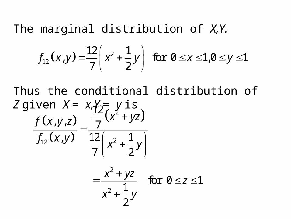
The marginal distribution of X,Y.

212

12 1, for 0 1,0 1

7 2f x y x y x y

Thus the conditional distribution of Z given X = x,Y = y is

2

212

12, , 7

12 1,7 2

x yzf x y z

f x yx y

2

2

for 0 112

x yzz

x y

1 2

22 1

20

,x yz

E U x y x y z dzx y

The conditional expectation of U = X 2 + Y + Z given X = x, Y = y.

1

2 22 1

2 0

1x y z x yz dz

x y

1

2 2 2 2 22 1

2 0

1yz y x y x z x x y dz

x y

13 2

2 2 2 22 1

2 0

1

3 2

z

z

z zy y x y x x x y z

x y

2 2 2 22 1

2

1 1 1

3 2y y x y x x x y

x y

Thus the conditional expectation of U = X 2 + Y + Z given X = x, Y = y.

2 2 2 22 1

2

1 1 1,

3 2E U x y y y x y x x x y

x y

2

2 2122 1

2

1

3 2

y xx y x y

x y

21 122 3

2 12

x yx y

x y

The rule for Conditional Expectation

E U E E U y y

Var U E Var U Var E U y yy y

Then

1 1Let , , , , , ,q mU g x x y y g x y

Let (x1, x2, … , xq, y1, y2, … , ym) = (x, y) denote q + m random variables.

Proof (in the simple case of 2 variables X and Y)

, ,E U g x y f x y dxdy

Thus ,U g X Y

, , X YE U Y E g X Y Y g x y f x y dx

,

,Y

f x yg x y dx

f y

hence

Y YE E U Y E U y f y dy

,

, YY

f x yg x y dx f y dy

f y

, ,g x y f x y dx dy

, ,g x y f x y dxdy E U

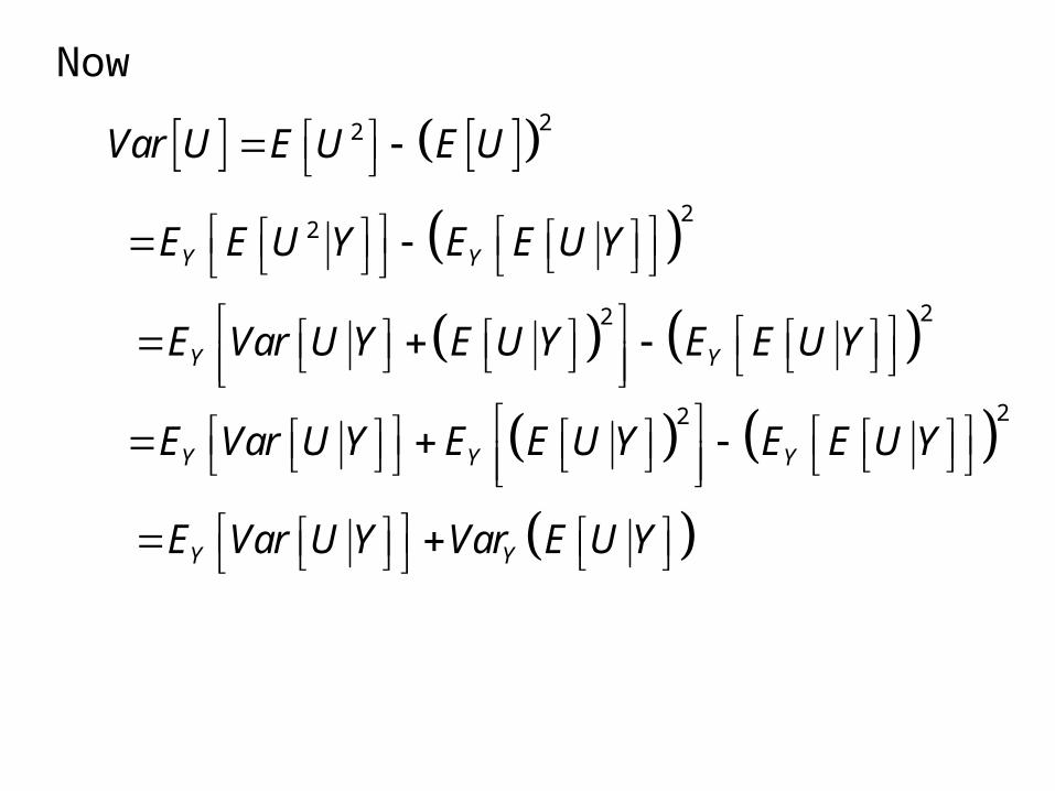
Now

22Var U E U E U

22Y YE E U Y E E U Y

22

Y YE Var U Y E U Y E E U Y

22

Y Y YE Var U Y E E U Y E E U Y

Y YE Var U Y Var E U Y

The probability of a Gamblers ruin

• Suppose a gambler is playing a game for which he wins 1$ with probability p and loses 1$ with probability q.

• Note the game is fair if p = q = ½. • Suppose also that he starts with an initial

fortune of i$ and plays the game until he reaches a fortune of n$ or he loses all his money (his fortune reaches 0$)

• What is the probability that he achieves his goal? What is the probability the he loses his fortune?

Let Pi = the probability that he achieves his goal?

Let Qi = 1 - Pi = the probability the he loses his fortune?Let X = the amount that he was won after finishing the gameIf the game is fair

Then E [X] = (n – i )Pi + (– i )Qi

= (n – i )Pi + (– i ) (1 –Pi ) = 0

or (n – i )Pi = i(1 –Pi )

and (n – i + i )Pi = iThus and 1i i

i i n iP Q

n n n

If the game is not fair

1 1then i i iP qP pP

1 1or since 1.i i ip q P qP pP p q

Thus 1 1 .i i i ip P P q P P

or 1 1 .i i i i

qP P P P

p

Note 0 0 and 1nP P

Also 2 1 1 0 1

q qP P P P P

p p

2

3 2 2 1 1

q qP P P P P

p p

3

4 3 3 2 1

q qP P P P P

p p

1

1 1

i

i i

qP P P

p

hence

2 1

1 1 1

iq q q

P P Pp p p

qr

p

1 2 1 3 2 1i i iP P P P P P P P

2 1

1 1 1 1

i

i

q q qP P P P P

p p p

or

2 11 1

11

1

ii r

P r r r Pr

where

Note

thus

1

11

1

n

n

rP P

r

1

1

1n

rP

r

1

1

1

i

i

rP P

r

and

1 1 1

1 1 1

i i

n n

r r r

r r r

1

1

iqp

nqp

tablei n p q P i Q i

9 10 0.50 0.50 0.900 0.1009 10 0.48 0.52 0.860 0.1409 10 0.45 0.55 0.790 0.2109 10 0.40 0.60 0.661 0.339

90 100 0.50 0.50 0.900 0.10090 100 0.48 0.52 0.449 0.55190 100 0.45 0.55 0.134 0.86690 100 0.40 0.60 0.017 0.983

900 1000 0.50 0.50 0.900 0.100900 1000 0.48 0.52 0.000 1.000900 1000 0.45 0.55 0.000 1.000900 1000 0.40 0.60 0.000 1.000

A waiting time paradox

• Suppose that each person in a restaurant is being served in an “equal” time.

• That is, in a group of n people the probability that one person took the longest time is the same for each person, namely 1

n• Suppose that a person starts asking people as they

leave – “How long did it take you to be served”.• He continues until it he finds someone who took

longer than himself

Let X = the number of people that he has to ask.

Then E[X] = ∞.

Proof 1

1P X x

x

= The probability that in the group of the first x people together with himself, he took the longest

p x P X x

1P X x P X x

1 1 1

1 1x x x x

Thus

1 1 1

1 1

1 1x x x

E X xp x xx x x

1 1 1 1

2 3 4 5

The harmonic series

1 1 1 1 1 1 1

2 3 4 5 6 7 8

The harmonic series

1 1 1 1 1 1 1

2 3 4 5 6 7 8

1 1 1 1 1 1 1

2 4 4 8 8 8 8

1 1 1

2 2 2